A short note on the entrainment and exit boundary conditions

INTERNATIONAL JOURNAL FOR NUMERICAL METHODS IN FLUIDSInt. J. Numer. Meth. Fluids 2006; 50:973–985Published online 17 October 2005 in Wiley InterScience (www.interscience.wiley.com). DOI: 10.1002/�d.1095

A short note on the entrainment and exit boundary conditions

P. Rajesh Kanna‡;§ and Manab Kumar Das∗;†;¶

Department of Mechanical Engineering; Indian Institute of Technology Guwahati; North Guwahati;Guwahati 781039; Assam; India

SUMMARY

An attempt is made to �nd out the suitable entrainment and exit boundary conditions in laminar �ow sit-uations. Streamfunction vorticity formulation of the Navier–Stokes equations are solved by ADI method.Two-dimensional laminar plane wall jet �ow is used to test di�erent forms of the boundary conditions.Results are compared with the experimental and similarity solution and the proper boundary conditionis suggested. The Kind 1 boundary condition is recommended. It consists of zero �rst derivative condi-tion for velocity variable and for streamfunction equation, mixed derivative at the entrainment and exitboundaries. Copyright ? 2005 John Wiley & Sons, Ltd.

KEY WORDS: entrainment; streamfunction; boundary conditions; plane wall jet

1. INTRODUCTION

Entrainment occurs when a jet of �uid �ows in an open domain. Flow over a �at plate,jet impingement on a plate, jet spread along a solid wall and jet emission into a quiescentdomain are few examples where entrainment occurs. It has wide industrial applications likeelectronics cooling, turbine blade cooling, defroster system and high speed engine cooling,etc. While solving the problem numerically in streamfunction vorticity formulation, there aremany ways to treat the boundary: few of them are Neumann boundary condition, Dirichletboundary condition and close form analytical expression. Vynnycky et al. [1] have followedan analytical expressions for stream function ( ) and vorticity (!) for solving �ow over a �atplate problem. They have considered the ‘e�ective in�nity’ to treat the entrainment condition.Angirasa [2] has used Dirichlet boundary condition for velocity component at in�nity forsolving buoyant wall jet. He used the gradients of stream function taken to be equal tozero on the free sides. This physically implies that far away from the walls, the �ow enters

∗Correspondence to: Manab Kumar Das, Department of Mechanical Engineering, Indian Institute of TechnologyGuwahati, North Guwahati, Guwahati 781039, Assam, India.

†E-mail: [email protected]‡E-mail: [email protected]§Research Scholar.¶Associate Professor.

Received 1 May 2005Revised 12 August 2005

Copyright ? 2005 John Wiley & Sons, Ltd. Accepted 13 August 2005

974 P. R. KANNA AND M. K. DAS

and leaves the computational domain normal to the boundary. Al-Sanea [3, 4] has followed�rst derivative equal to zero as exit boundary condition for treating continuously movingplate problem. For entrainment velocity calculations its value depends upon the mass �owrate drawn outside the calculation domain by the viscous action of the moving plate. Hanet al. [5] have investigated a discrete arti�cial boundary condition in stream function andvorticity formulation. They tested a few problems, viz. channel �ow, �ow over an obstacle,�ow over backward facing step and �ow over forward facing step problem and comparedwith Dirichlet and Neumann boundary conditions. Finally they concluded from the numericalresults obtained that the boundary condition is very e�ective. Rao et al. [6] have used crossderivative for stream-function at entrainment and they have used potential �ow, i.e. vorticityas zero value while solving mixed convection along �at plate. The present work is originatedfrom the reviewer’s comments of Kanna and Das [7] about the treatment of entrainment andexit boundary condition for an o�set jet �ow.The present investigation is concerned about �nding a suitable form to treat the entrainment

and exit boundary condition. The study is carried out with an example problem of two-dimensional laminar incompressible plane wall jet �ow. When a jet of �uid issues from a slitand spread along a wall, it forms a wall jet. It has inner region which behaves like a boundarylayer �ow over a �at plate and outer region behaves like a free shear layer [8]. The similaritypro�le has a point of in�exion. Glauert [9] has presented close form solution for plane wall jetof laminar as well as turbulent �ow. Quintana et al. [10] have reported experimental resultsfor laminar plane wall jet where surrounding is quiescent. Similar situation is considered forthe present investigation of wall jet �ow.

2. MATHEMATICAL FORMULATION

An incompressible two-dimensional laminar plane wall jet is considered. For the sake ofsimplicity, the jet is assumed to be isothermal and having the same density as the ambient�uid. Also, the velocity pro�le at the jet inlet is taken as parabolic. The schematic of theproblem is shown in Figure 1 and the boundary conditions are shown in Figure 2. Theboundary layer thickness � is de�ned as the normal distance from the wall upto the distancewhere the velocity is half of local u maximum.The governing equations for incompressible laminar �ow are solved by stream function-

vorticity formulation. The transient non-dimensional governing equations in the conservativeform areStream function equation:

∇2 = − ! (1)

Vorticity equation:

@!@t+

@(u!)@x

+@(v!)@y

=1Re

∇2! (2)

where -stream function, u= @ @y ; v= − @

@x and != @v@x − @u

@y .

Copyright ? 2005 John Wiley & Sons, Ltd. Int. J. Numer. Meth. Fluids 2006; 50:973–985

ENTRAINMENT AND EXIT BOUNDARY CONDITIONS 975

x

y

u = v = 0

u =

v =

0

u (y)

δ

UmGeometry and boundary conditons

Configuration of Wall Jet

Um/2

h

Figure 1. Schematic diagram and similarity pro�le of wall jet.

u = v = 0

u =

v=

0

u(y)

B

CD

A

E

Figure 2. Boundary conditions in a plane wall jet problem.

The variables are scaled as

u=�u�U; v=

�v�U; x=

�xh; y=

�yh; !=

�!�U=h; t=

�th= �U

with the overbar indicating a dimensional variable and �U; h denoting the average jet velocityat nozzle exit and the jet width, respectively.The boundary conditions needed for the numerical simulation have been prescribed. For

plane wall jet with entrainment, the following dimensionless conditions have been enforcedas shown in Figure 2. The inlet slot height is assumed as h=0:05.At the jet inlet, along AE (Figure 2)

u(y)=120y − 2400y2; !(y)=4800y − 120; (y)=60y2 − 800y3 (3a)



Along AB and ED due to no-slip condition

u= v=0 (3b)

Along DC

@u@y=0 or

@v@y=0 or v=0 (3c)

At downstream boundary, the condition of zero �rst-derivative has been applied for velocitycomponents. This condition implies that the �ow has reached a developed condition. Thus, at(BC)

@u@x=

@v@x=

@!@x=0 (3d)

Similar type of boundary conditions have been used by Al-Sanea [3, 4]. For comparison andvalidation with available experimental and numerical work, two cases namely, plane wall jetand plane sudden-expansion �ow problems have been solved. In the second case, all the wallsexcept the inlet and the outlet are solid. Thus there is no entrainment from the atmosphereand the boundary conditions are no-slip for these surfaces.

3. NUMERICAL PROCEDURE

The unsteady vorticity transport equation (2) in time is solved by alternate direction implicitscheme (ADI). Solution approaches steady-state asymptotically while the time reaches in�nity.The computational domain considered here is clustered Cartesian grids. For unit length, thegrid space at ith node is [11]

xi=(

iimax

− �#sin

(i#imax

))(4)

where # is the angle and � is the clustering parameter. #=2� stretches both end of the domainwhereas #=� clusters more grid points near one end of the domain. � varies between 0 to1. When it approaches 1, more points fall near the end.The central di�erencing scheme is followed for both the convective as well as the di�usive

terms [12]. It consists of two half time-steps. For details of the disctretization procedure,readers are referred to the article Kanna and Das [7].The velocity components are updated by the following equations:

u=@ @y=

i; j+1 − i; j−1�yj +�yj−1

(5a)

v=−@ @x=

i+1; j − i−1; j�xi +�xi−1

(5b)



The velocities are calculated at nth time level while advancing to the (n+1)th time level.Because of this approximation in the nonlinear terms, the second-order accuracy of the methodis somewhat lost. However, something of the second-order accuracy of the linearized systemis retained if the velocity �eld is slowly varying [12].It is �rst-order accurate in time and second-order accurate in space O(�t;�x2;�y2), and

is unconditionally stable. The streamfunction equation (1) is solved explicitly by �ve pointGauss–Seidel methods. Thom’s vorticity condition has been used to obtain the wall vorticityas given below

!w= − 2( w+1 − w)�n2

(6)

where �n is the grid space normal to the wall. It has been shown by Napolitano et al. [13]and Huang and Wetton [14] that convergence in the boundary vorticity is actually second-order for steady problems and for time-dependent problems when t ¿ 0. Roache [12] hasreported that for a Blausius boundary-layer pro�le, numerical test veri�es that this �rst-orderform is more accurate than second-order form.At the bottom wall and the left side wall, constant stream lines are assumed based on inlet

�ow. At the outlet in the downstream direction, streamwise gradients are assumed to be zero.At the entrainment boundary, normal velocity gradient is zero [15].The detailed boundary conditions are

Along ED (Figure 2):

!(y)=2( w − w+1)�x1 ∗ �x1

; =0:05 (7a)

Along AB:

!(x)=2(0− w+1)�y1 ∗ �y1

; =0 (7b)

Entrainment boundary (DC) and exit boundary (BC) are tested by di�erent form of bound-ary conditions namely Kind I, Kind II and Kind III.Kind 1:

Along DC

@2 @x@y

=0(from

@v@y=0; Equation (3c)

)(8a)

Discretizing Equation (8a) we get

i; j= i−1; j + i; j−1 − i−1; j−1 (8b)

From the condition (Equation (3c))

@u@y=0; ui; j= ui; j−1 (8c)

vi; j =− ( i+1; j − i−1; j)�xi +�xi−1

(8d)



!i; j =(vi+1; j − vi−1; j)(�xi +�xi−1)

(8e)

Along BC, !; u; v, are evaluated based on zero gradient in the streamwise direction [12].Backward di�erence scheme is followed for the �rst derivative at exit.

@2 @x@y

=0(from

@u@x=0; Equation (3d)

)(8f)

Discretizing Equation (8f)

i; j = i−1; j + i; j−1 − i−1; j−1 (8g)

!i; j =!i−1; j (8h)

ui; j = ui−1; j (8i)

vi; j = vi−1; j (8j)

Kind 2:Along DC ; u; v and ! are evaluated as follows:

@2 @x@y

=0(from

@v@y=0; Equation (3c)

)(9a)

Discretizing Equation (9a), we get

i; j = i−1; j + i; j−1 − i−1; j−1 (9b)

ui; j = ui; j−1

(from

@u@y=0; Equation (3c)

)(9c)

vi; j =−@ @x= − ( i+1; j − i−1; j)

�xi +�xi−1(9d)

!i; j =(vi+1; j − vi−1; j)(�xi +�xi−1)

(9e)

Along BC, !; u; v, are evaluated based on streamwise direction �rst gradient is zero [12].Backward di�erence scheme is followed for the �rst derivative at exit.

@2 @x2

= 0(from

@v@x=0; Equation (3d)

)(9f)

Discretizing Equation (9f)

i; j = 2 i−1; j − i−2; j (9g)



!i; j =!i−1; j (9h)

ui; j = ui−1; j (9i)

vi; j = vi−1; j (9j)

Equation (9f) is suggested by Roache [12] based on @v=@x=0.Kind 3:

Along DC

@u@y=0 (10a)

ui; j = ui; j−1 (10b)

vi; j =0 (10c)

from Equation (10c)

i; j = i−1; j (10d)

!i; j =(vi+1; j − vi−1; j)(�xi +�xi−1)

(10e)

Along BC, !; u and v are evaluated by Equations (8h)–(8j). is evaluated by (9f) and(9g).Along DC, Kind 1 and Kind 2 boundary expressions are common for !; ; u and v. Kind 3

is di�erent for v (Equation (10c)) and thus expression is also di�erent from Kind 1 andKind 2. Along BC for !; u; v Kind 1 is followed which is �rst-order accurate discretizationbased on �rst derivative equal to zero. Roache [12] suggested that �rst-order accurate termsare giving better results than second-order accurate approximation for the situations consideredhere. For second-order accurate approximation is followed based on Equation (3d) ( @u@x =0).In case of Kind 2, is calculated based on Equation (3d) ( @v@x =0). For !; u and v, Kind 2is identical with Kind 1. In case of Kind 3 along BC, !; u and v are evaluated by Equations(8h)–(8j). Evaluation of is performed by (9f) and (9g). These combinations of threeboundary conditions for entrainment and exit situations are tested.The maximum vorticity error behaviour is complicated as explained by Roache [12]. While

marching in time for the solution, it has been observed that the maximum vorticity errorgradually decreases. It then increases drastically and �nally decreases asymptotically leadingto steady-state solution. The convergence criteria is to be set in such a way that it should notterminate at false stage. At steady state, the error reaches the asymptotic behaviour. Here itis set as sum of vorticity error (Equation (11)) reduced to either the convergence criteria �or elapsed large total time

imax ; jmax∑i; j=1

|(!t+�ti; j − !t

i; j)| ¡ � (11)



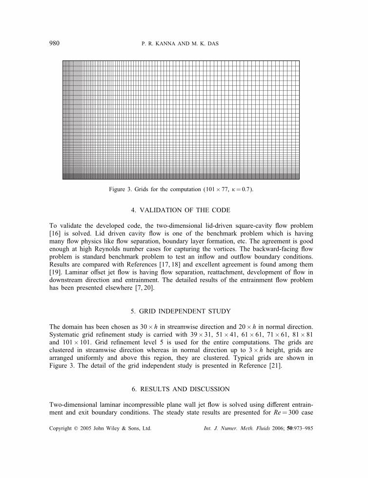
Figure 3. Grids for the computation (101× 77, �=0:7).

4. VALIDATION OF THE CODE

To validate the developed code, the two-dimensional lid-driven square-cavity �ow problem[16] is solved. Lid driven cavity �ow is one of the benchmark problem which is havingmany �ow physics like �ow separation, boundary layer formation, etc. The agreement is goodenough at high Reynolds number cases for capturing the vortices. The backward-facing �owproblem is standard benchmark problem to test an in�ow and out�ow boundary conditions.Results are compared with References [17, 18] and excellent agreement is found among them[19]. Laminar o�set jet �ow is having �ow separation, reattachment, development of �ow indownstream direction and entrainment. The detailed results of the entrainment �ow problemhas been presented elsewhere [7, 20].

5. GRID INDEPENDENT STUDY

The domain has been chosen as 30× h in streamwise direction and 20× h in normal direction.Systematic grid re�nement study is carried with 39× 31, 51× 41, 61× 61, 71× 61, 81× 81and 101× 101. Grid re�nement level 5 is used for the entire computations. The grids areclustered in streamwise direction whereas in normal direction up to 3× h height, grids arearranged uniformly and above this region, they are clustered. Typical grids are shown inFigure 3. The detail of the grid independent study is presented in Reference [21].

6. RESULTS AND DISCUSSION

Two-dimensional laminar incompressible plane wall jet �ow is solved using di�erent entrain-ment and exit boundary conditions. The steady state results are presented for Re=300 case



(a) (b)

(c)

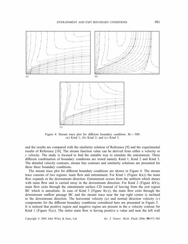
Figure 4. Stream trace plot for di�erent boundary condition: Re=300:(a) Kind 1; (b) Kind 2; and (c) Kind 3.

and the results are compared with the similarity solution of Reference [9] and the experimentalresults of Reference [10]. The stream function value can be derived from either u velocity orv velocity. The study is focused to �nd the suitable way to simulate the entrainment. Threedi�erent combination of boundary conditions are tested namely Kind 1, Kind 2 and Kind 3.The detailed velocity contours, stream line contours and similarity solutions are presented forthese three boundary conditions.The stream trace plot for di�erent boundary conditions are shown in Figure 4. The stream

trace consists of two regions: main �ow and entrainment. For Kind 1 (Figure 4(a)) the main�ow expands in the downstream direction. Entrainment occurs from the ambient which shearswith main �ow and is carried away in the downstream direction. For Kind 2 (Figure 4(b)),main �ow exits through the entrainment surface CD instead of leaving from the exit regionBC which is unrealistic. In case of Kind 3 (Figure 4(c)), the main �ow exits through thedownstream out�ow passage BC and the stream trace near the top right corner is inclinedto the downstream direction. The horizontal velocity (u) and normal direction velocity (v)components for the di�erent boundary conditions considered here are presented in Figure 5.It is noticed that positive region and negative region are present in the u velocity contour forKind 1 (Figure 5(a)). The entire main �ow is having positive u value and near the left wall



.5050

0.265

0.170

0.075

0.021-0.002

-0.000

0.000

-0.016

0.075

-0.056

-0.051

-0.030

0.129

0.076 0.05

0

0.023

0.004

0.5430.352

0.256

0.161

0.065

0.020

-0.015

-0.000-0.000

-0.004

0.001

-0.015 -0.015

0.1820.103

0.103

0.129

0.0010.005

0.023

0.050

0.076

-0.056

-0.056

-0.030-0.030

-0.003

0.153

0.5500.360

0.265

0.170

0.136

0.075

0.053

0.031

0.01

0-0.002-0.006

-0.009

0.003

0.001

0.150 0.10

4

0.08

0

0.05

7

0.034 0.021

0.011

0.003

0.011

-0.013

-0.036-0.036

-0.059

-0.048(a) (b)

(c) (d)

(e) (f)

Figure 5. Velocity contour: Re=300: (a) u velocity contour: Kind 1; (b) v velocity contour: Kind1; (c) u velocity contour: Kind 2; (d) v velocity contour: Kind 2; (e) u velocity contour: Kind 3;

and (f) v velocity contour: Kind 3.

negative u contours are present. Due to the pressure di�erence, �ow occurs towards the entryof the jet. It is observed that near the boundary DC, u is approaching zero value. Figure 5(b)shows the v velocity contour for Kind 1 boundary condition. It is noticed that positive v value



u/umax

η

0 0.25 0.5 0.75 1

1

2

3

4

5

6

7

8

Kind 1Kind 2Kind 3

η

0 0.25 0.5 0.75 10

0.5

1

1.5

2

2.5

3

Kind 1Kind 2Kind 3ExperimentSimilarity solution




η

0 0.25 0.5 0.75 10

0.5

1

1.5

2

2.5

3

3.5

η

0 0.25 0.5 0.75 10

0.25

0.5

0.75

1

1.25

1.5

1.75

2

2.25

2.5

2.75

3

3.25

3.5

η

0 0.25 0.5 0.75 10

0.5

1

1.5

2

2.5

3

3.5

u/umax

u/umax

u/umax

u/umax

(a) (b)

(c) (d)

(e)

Figure 6. Similarity pro�le from di�erent downstream location: Re=300, experiment results by Quintanaet al. [10]: (a) x=3h; (b) x=10h; (c) x=15h; (d) x=20h; and (e) x=25h.



occurs at the main �ow and negative values occur around entrainment. By the magnitude ofthe velocity near the entrainment boundary DC and exit boundary BC, it is observed that v ishigher than u near the DC and u is higher than v near BC. For Kind 1 case, the streamfunctionis evaluated based on these equations: along DC is evaluated from @v=@y=0 and along BCit is evaluated from @u=@x=0. The u velocity contour and v velocity contour are presentedfor Kind 2 in Figures 5(c) and 5(d). Negative u velocity value is observed near the exitand positive v velocity is observed at the entrainment boundary. The u velocity contour ispresented in Figure 5(e) for Kind 3. The main �ow and entrainment along DC are simulatedwell by Kind 3 when compared with Kind 2. However, near the corner D positive u velocityis present. Close to a constant value is obtained for v velocity near DC which is parallel tothe top entrainment surface (Figure 5(f)).The boundary layer thickness (�) is de�ned (Figure 1) as the normal distance where velocity

is equal to um=2 and similarity variable (�) is de�ned as y=�. Similarity pro�le at di�erentdown-stream location is shown in Figure 6. At x=3h, the three boundary conditions areyielding the same velocity pro�le results (Figure 6(a)). The pro�le is having a small negativeregion at the shear layer of main �ow with entrainment. Further downstream direction atx=10h, the jet is expanded in the normal direction (Figure 6(b)). Results are compared withthe similarity solution [22] and experimental results of Quintana et al. [10]. It is noticed thatfor Kind 1 and Kind 2, the velocity pro�le is having good agreement with them whereas forKind 3, it is having good agreement with them upto certain distance in the outer region. Faraway in the normal direction, it starts to deviate in the negative direction from the benchmarkresults. Figure 6(c) shows the similarity velocity pro�le at x=15h location. For Kind 1and Kind 2, the velocity pro�les are having good agreement with available results. In case ofKind 3 the velocity pro�le slightly deviates in the entrainment region. At x=20h, the velocitypro�le Kind 1 is still having better agreement with standard benchmark results (Figure 6(d))whereas for Kind 2 and Kind 3, the velocity pro�les di�er signi�cantly from them. Thesimilarity pro�le at x=25h location is shown in Figure 6(e). Kind 1 boundary condition hascaptured the wall jet similarity pro�le. Kind 2 has led to a reverse �ow near the solid wall andum location is shifted in the normal direction compared to the benchmark similarity solution.For Kind 3, the velocity pro�le is having agreement with benchmark results upto part of theouter region and further in the normal direction it deviates and has constant u=um value whichis higher than the benchmark value.

7. CONCLUSIONS

Numerical experiments are carried out to �nd the suitable entrainment and exit boundaryconditions for laminar incompressible viscous �ow situation. Stream function vorticity formu-lation of the governing equations are solved by ADI method. Two-dimensional laminar planewall jet �ow is considered for the study and the following conclusions are drawn. Near theentrainment boundary magnitude of normal direction velocity component is higher than thestreamwise velocity component. Near the exit boundary, streamwise velocity component ishigher than the normal direction velocity component. Streamfunction can be evaluated fromeither u or v velocity component. For boundary condition Kind 1, the velocity which hashigher magnitude value is used. It shows excellent agreement with experimental as well assimilarity solution. Kind 2 leads to erroneous results in the �ow �eld. Reverse �ow is observed



in the similarity pro�le. Authors feel that for entrainment like situation Kind 1 boundary con-dition is suitable to capture the �ow physics. It consists of zero �rst derivative condition forvelocity variable and for streamfunction equation, mixed derivative at the entrainment andexit boundaries.

ACKNOWLEDGEMENTS

The helpful comments of the reviewers are sincerely acknowledged by the authors.

REFERENCES

1. Vynnycky M, Kimura S, Kanev K, Pop I. Forced convection heat transfer from a �at plate: the conjugateproblem. International Journal of Heat and Mass Transfer 1998; 41:45–59.

2. Angirasa D. Interaction of low-velocity plane jets with buoyant convection adjacent to heated vertical surfaces.Numerical Heat Transfer, Part A 1999; 35:67–84.

3. Al-Sanea SA. Convection regimes and heat transfer characteristics along a continuously moving heated verticalplate. International Journal of Heat and Fluid Flow 2003; 24:888–901.

4. Al-Sanea SA. Mixed convection heat transfer along a continuously moving heated vertical plate with suction orinjection. International Journal of Heat and Mass Transfer 2004; 47:1445–1465.

5. Han H, Lu J, Bao W. A discrete arti�cial boundary condition for steady incompressible viscous �ows in ano-slip channel using a fast iterative method. Journal of Computational Physics 1994; 114:201–208.

6. Rao CG, Balaji C, Venkateshan SP. Conjugate mixed convection with surface radiation from a vertical platewith a discrete heat source. Journal of Heat Transfer 2001; 123:698–702.

7. Kanna PR, Das MK. Numerical simulation of two-dimensional laminar incompressible o�set jet �ows.International Journal for Numerical Methods in Fluids 2005; 49(4):439–464.

8. Bajura RA, Szewczyk AA. Experimental investigation of a laminar two-dimensional plane wall jet. Physics ofFluids 1970; 13:1653–1664.

9. Glauert MB. The wall jet. Journal of Fluid Mechanics 1956; 1(1):1–10.10. Quintana DL, Amitay M, Ortega A, Wygnanski IJ. Heat transfer in the forced laminar wall jet. Journal of Heat

Transfer 1997; 119:451–459.11. Kuyper RA, Van Der Meer ThH, Hoogendoorn CJ, Henkes RAWM. Numerical study of laminar and turbulent

natural convection in an inclined square cavity. International Journal of Heat and Mass Transfer 1993;36(11):2899–2911.

12. Roache PJ. Fundamentals of Computational Fluid Dynamics, Chapter 3. Hermosa: U.S.A, 1998.13. Napolitano M, Pascazio G, Quartapelle L. A review of vorticity conditions in the numerical solution of the

� − equations. Computers and Fluids 1999; 28:139–185.14. Huang H, Wetton BR. Discrete compatibility in �nite di�erence methods for viscous incompressible �uid �ow.

Journal of Computational Physics 1996; 126:468–478.15. Kang SH, Greif R. Flow and heat transfer to a circular cylinder with a hot impinging air jet. International

Journal of Heat and Mass Transfer 1992; 35(9):2173–2183.16. Ghia U, Ghia KN, Shin CT. High resolutions for incompressible �ow using the Navier–Stokes equations and

multigrid method. Journal of Computational Physics 1982; 48:387–411.17. Armaly BF, Durst F, Pereira JCF, Schonung B. Experimental and theoretical investigation of backward-facing

step �ow. Journal of Fluid Mechanics 1983; 127:473–496.18. Gartling DK. A test problem for out�ow boundary conditions-�ow over a backward-facing step. International

Journal for Numerical Methods in Fluids 1990; 11:953–967.19. Kanna PR, Das MK. A note on the reattachment length for BFS problem. International Journal for Numerical

Methods in Fluids 2005, in press.20. Kanna PR, Das MK. Numerical simulation of two-dimensional laminar incompressible wall jet under backward-

facing step �ows. Journal of Fluids Engineering 2005, submitted.21. Kanna PR, Das MK. Conjugate forced convection heat transfer from a �at plate by laminar plane wall jet �ow.

International Journal of Heat and Mass Transfer 2005; 48:2896–2910.22. Schlichting H, Gersten K. Boundary Layer Theory (8th edn). Springer: Berlin, 2000; 215–218.


A short note on the entrainment and exit boundary conditions

Documents

Transcript of A short note on the entrainment and exit boundary conditions