IEEE Transaction on Power Apparatus and Systems, Vol. PAS-104, No. 1, January 1985

DISTRIBUTION TRANSFORMER NO-LOAD LOSSES

D. S. Takach, Senior Member, IEEEWestinghouse Electric CorporationJefferson City, Missouri

Abstract - This paper considers the subject ofdistribution transformers no-load losses and thefactors that influence these losses. This paperreviews methods to correct errors in no-load lossmeasurement caused by excitation voltage distortionand temperature. These methods depend on the abilityto separate no-load losses into its hysteresis andeddy current loss components. Accordingly, methodsused to separate the no-load losses into itsconstituent parts are also reviewed. Commentsregardings the application of loss separation totransformer cores, as opposed to Epstein samples, areincluded to serve as a basis for futureinvestigations.

INTRODUCTION

The subject of losses in electrical machinery,particularly losses associated with electrical steelused in this machinery, has gained in importance Inthe last several years due to the dramatic increasein the cost of producing these losses. As of 1977,the estimate of electrical steel losses found intransformers alone approached 41 x 109 kWHr, and ifthe energy cost is assumed to be $0.03/kWHr, thetotal yearly cost of these losses is $1.23billion1l]. In 1977, utilities, on the average,evaluated transformer no-load loss, on an equivalentinvestment cost basis, at about $16001kW. Currently,the -average evaluation on an equivalent investmentcost is about $4,000/kW with some evaluationsapproaching $13,500/kW. Thus, in some cases, theevaluated cost of a transformer's no-load loss canwell exceed the first cost of the transformeritself. So, the subject of transformer no-loadlosses, the factors that influence them, and theirmeasurement become important subjects.

Transformer no-load losses are sensitive to atransformer's operating environment. Any distortionof the exciting voltage and variation in coretemperature can change the no-load losses from whatthey would be at standard operating conditions,i.e., sinusoidal excitation and a no--load lossreference temperature. Transformer manufacturingprocessing may expose the transformer's core tovarying conditions at the time of test. For example,processing of a transformer's windings may leave thetransformer core temperature elevated with respect toambient conditions at the time of test producingdifferent no-load losses than those measured atambient conditions. Transformer test facilities,generally, have power supplies and metering equipmentdiffering in impedance producing different amounts ofexcitation voltage waveform distortion, againchanging the measured no-load losses from the lossesobserved under purely sinusoidal excitation. Formoderate values of temperature variance and

84 T&D 390-1 A paper recommended and approvedby the IEEE Transformers Committee of the IEEEPower Engineering Society for presentation at theIEEE/PES 1984 Transmission and DistributionConference, Kansas City, Missouri, April 29 - May4, 1984. Manuscript submitted November 2, 1983;made available for printing March 5, 1984.

R. L. Boggavarapu, Member, IEEEWestinghouse Electric CorporationPittsburgh, Pennsylvania

excitation voltage waveform distort'ion the correctionto the magnitude of the no-load loss measured issmall. The evaluated cost of those smallcorrections, however, is not insignificant.Therefore, the test conditions must be properlyaccounted for when correcting measured no-load lossvalues to standard reference conditions.

This paper presents a review of the fundamentalcomponents of distribution transformer no-load loss,the methods used to correct no-load loss to standardreference conditions, and the methods used toseparate no-load loss into its component parts.

GENERAL REVIEW OF NO-LOAD LOSS

The losses measured under no-load conditions intransformers consist of hysteresis and eddy currentlosses in core laminations, I2R loss in thewindings due to the no-load current, stray eddycurrent losses in core clamps, bolts, etc., of thecore structure, losses due to interlaminar flux (fluxcrossing from one lamination to the next), anddielectric losses which become important fortransformers with voltages exceeding 50 kv[2].Methods for accurate measurement of these losses,along with problems that may be encountered intransformers, are described in the literature13].

The no-load current in distribution transformers,with the type of joints and wound-core constructionused throughout the industry, is generally about 1%to 2% of the rated full-load current. The 12R lossdue to this current can be considered negligible.The distribution transformers do not have voltagesapproaching 50kv and, hence, dielectric losses can beneglected. Thus, the no-load losses measured duringtest can be assumed to consist essentially of corelosses, i.e., hysteresis and eddy current losses Incore laminations. Eddy current losses deduced fromthe separation of losses, described in a subsequentsection, are generally higher than those calculatedfrom the classical theory. The difference betweenmeasured total losses and the sum of the hysteresisand calculated eddy current losses is termed the"anomalous" loss. The anomalous loss can amount toas much as 50% of the measured losses ingrain-oriented 3% Si-Fe steels41. These threelosses, hysteresis, eddy current and anomalouslosses, and the parameters on which they depend aredescribed briefly.

Ferromagnetism[5 1

Some of the common ferromagnetic materials areiron, cobalt, nickel, and many alloys containing oneor more of these metals. A sample of iron is knownto be composed of many small regions, or domains,each magnetized to saturation in some direction andhaving dimensions of approximately 10-5 meter. Theflux density in the domains Is large, and is of theorder of two webers/meter2. The domains arenormally oriented in such a way that the externalmagnetic field is zero, for this condition givesminimum stored energy. There is energy stored in theinternal field, and there is also energy associatedwith the domain walls and with the direction ofmagnetization relative to the crystal areas.

0018-9510/85/0001-0181$01.00O1985 IEEE

181

182

The behavior of domain walls as a specimen ismagnetized can be observed under the microscope byplacing a drop of colloidal suspension offerromagnetic particles on a prepared surface. Theparticles congregate near the domain boundaries dueto the presence of strong magnetic fields. When amagnetizing force, H, is applied, the walls move.The walls tend to cling to impurities, strains, andother imperfections that are present. Hence, thewall motion is irregular, causing the magnetizationto increase irregularly. This is known as theBarkhausen effect, which can be detected by wrappinga sample being magnetized with a coil of wireconnected through an amplifier to a loudspeaker. Aseries of audible clicks can be heard, resulting fromthe small abrupt changes in the flux density, thatproduce voltage pulses in the coil. The boundariesmove in such a way that those domains that are

spontaneously magnetized in the approximate directionof the applied field grow at the expense of others.The process continues as the applied field isincreased until saturation is reached, with thesample essentially one large domain. There is alsosome domain rotation at the higher field strengths.

BSATURATM

In the region above the knee of the magnetizationcurve, the increase in the magnetization is duemostly to domain rotation. When saturation isreached, all the domains are aligned with H, and nofurther increase in the magnetization is possible.

Hysteresis Loss

If the magnetizing force applied to aferromagnetic specimen is increased to saturation andis gradually reduced again to zero, the return B-Hcurve does not retrace the initial curve, but liesabove it (Figure 2)[61. This lag in thedemagnetization is a consequence of inclusions thatimpede the motion of domain walls, earlier referredto as irreversible boundary displacement. Thiseffect is called hysteresis. The finite value of Bwhen H Is zero, OR in Figure 2 is called the residualflux density (or remanence, Br). To demagnetize thespecimen completely, it Is necessary to apply anegative magnetizing force represented by OC. Thisis called coercive force, HC. If the magnetizingforce is increased in this direction, saturation inthe opposite direction is obtained. (Point D inFigure 2). If, finally, the magnetizing force isgradually reduced to zero, reversed, and increased toits maximum value in the original direction, thecurve DEFA will be traced out. The complete curveforms a closed loop called a hysteresis loop. It canbe seen that to take the specimen through the variousstates represented by this loop, an alternatingmagnetizing force is required. If these alterationsare maintained, and the maximum value of BM inFigure 2 is the same during each cycle, the specimenwill continue to go through the same series ofchanges.

2(WEBERS/METER)

Fig. 1 Typical Magnetization Curve

The net magnetization of a ferromagnetic specimenis a non-linear function of the applied field, H. Atypical magnetization curve is shown in Figure 1,with the origin showing the unmagnetized state. Whena magnetizing force is gradually increased from zero

by a small amount, the domain walls move, producing a

net flux density. The walls that respond initiallyare mainly those not held by imperfections, and thismovement i's reversible. There is also some

reversible domain rotation. If the applied field isreduced to zero, the return path followsapproximately the same magnetization curve, and thereis little energy loss. The slope of themagnetization curve at the origin is called initialpermeability.

C

A

H

(AMPERES/METER)

E

DIFig. 2Typical Hysteresis Loop for Ferromagnetic Materials

As the magnetizing force is further increased,the flux density rises more rapidly, and the slope ofthe magnetization curve between the origin and theknee is relatively steep. In this region of easymagnetization, the wall movement is largelyirrevers'ible. The stronger applied f'ield enables thewalls to move through imperfections with irregularmotion and an expenditure of energy. If themagnetizing force is reduced, the return path doesnot follow the same magnetization curve. Maximumabsolute permeability is obtained near the knee ofthe curve.

The hysteresis loop can be regarded as a magneticindicator diagram. During each cycle, an amount ofenergy represented by the area enclosed by the loopis expended. This is shown as follows:

Suppose the specimen is a ring of meancircumference, 1, in meters, and cross-sectionalarea, A, in meters2. Assume that a coil of N turnsis wound over the specimen. If the value of themagnetizing current at any instant of time, t, inseconds is, i, in amperes, then the magnetizing forceH is given by equation (1).

183

H = Ni ampere turn (1)1 meter

If the value of the indu'ction at the instantconsidered Is B, then the induced voltage, e, in thecoil is given by equation (2).

e = Nd4 = NAdBdt 'dt

volts

The current, i, flowing at that instant will beopposed by this induced'voltage, and therefore, powerwill have to 'be expended' in order to maintain theincrease in current. This required power is given byequation (3).

Power at any instant = ei = lAHdB watts (3)dt

Work done in time dt = lAHdBdt joules (4)dt

The eddy current losses can be calculated, usingclassical theory, as followst6]. Consider a volumeelement of a lamination of thickness, d, in meters,and length and depth of 1 meter each as shown inFigure 3. The maximum flux density, BM, in thedirection shown is% pulsating sinusoidally at afrequency of f cycles per second. The flux throughan area bounded by the shaded differential element is2xBM. The voltage induced by: the pulsating flux isgiven by equation (7).

e (instantaneous) =didt

E (RKS)

= d (2xBN sinwt)dt

= 2w f(2xBH) volts{2

(7)

(8)

The current in the strips dx, up one side and down onthe other side, is given by equation (9).

Total work done for = lA#HdB,one cyclp

joules (5)

It can be seen from Figure 2 that HdB is theof an elementary strip of the B-H curve',therefore, 4HdB (for. an entire cycle) is theenclosed by' ,the loop. The volume of thespecimen is UA.-

Work done = Area of loop (joules)meter-,

Eddy Current Loss

areaand

arearing

(6)

A time-changing magnetic f ield in a conductingsolid, either {ferromagnetic or non-ferromagnetic,produces" an induced voltage around each closed paththat encircles lines 'of magnetic flux. CirculatingcurrentEs, induced ih the conductor by these. voltagesare known as- eddy currents,' and the result-ing heatlosses, 'as a rule, are undesirable. 'In an effort, tominimize Fthese, losses' in transformers, magneticmaterial' made of "thin sheets,.'or laminations,- areused. These laminations are insulated; from oneanother and placed (parallel to the'flux.

Where plaminationdissipated

I1= 1 8 _EdiP2 2pdx

is the electrical resistivity ofmaterial in ohm-meters. Power,

in the differential element, dx, is:

2 2 2 2Pdx RI =(4fB ) x dxdx

(9)

thePdxa

(10)

-1pThe power, P, dissipated in the lamination is:

d/2 Id/2P =

0 dPx dx = (4wf2BN2)olx2dxp

=w f .Bd

6p -,

and since the volume of , thein meter3 the eddy currentPee' becomes

watts (11)

element considered is dloss per unit volume,

2 ~~~~~~3Pec = (WfBd2 watts/meter (12)

6pIt is to be noted that the eddy current loss 'is

proportional to the square of the thickness, d, ofthe laminations. In electrical machines the eddycurrent losses are minimized by the use of laminatedmaterial having higher resistivity. Silicon steelhas a resistivity several times greater than ordinarysheet steel.

If the closed B--H curve of a laminatedferromagnetic material is obtained with analternating magnetizing force, the area of the loopequals the. total core loss per unit volume percycle. This core loss is, of course, the sum .of thehysteresis and eddy current losses. The hysteresisloss is proportional to frequency and maximum fluxdensity. The eddy current loss is proportional tothe square of the frequency, at least in classicaltheory.

Fig. 3 Eddy Current

1-

Loss,Calculation

AONMALOUS LOSS

EDDY CURRENT LOSS

STATIC HYSTERESIS LOS

FREQUENCY

no-load condition is intended as a review. Theemphasis in this paper is to be able to correct themeasured no--load losses to a standard base forcomparison and evaluation of products from differentmanufacturers and different test conditions.Although It is important from the fundamental pointof view and for developing better magnetic materialsto divide the losses into three components asdescribed above, the common practice is to divide theno-load loss into hysteresis and eddy currentlosses. The latter include the classical eddycurrent losses and the anomalous losses.

The ratio of hysteresis to eddy current losses,for a given material, is a function of temperature,frequency, and maximum flux density, BK. Variousmethods for applying correction for temperature andeffects of distorted waveform willl be reviewed in thefollowing sections.

WAVEFORM DISTORTION EFFECTS

Fig. 4 Division of Total No-Load Loss Into ItsComponents

Anomalous Loss

It is to be noted that the classical eddy currentloss is calculated assuming that the material ishomogenous and has constant permeability, and theflux penetrates fully into the laminations. In orderto determine the methods to reduce these losses, ithas become customary to separate the .measured totallosses into hysteresis and eddy current components.

The total loss per cycle plotted againstfrequency is shown in Figure 4. This is obtained bymeasuring the power loss over the frequency range of20 Hz to 1000 Hz and extrapolating the characteristicto zero frequency. The classical eddy current lossis calculated from equation (12). The sum of theextrapolated hysteresis loss and the calculatedclassical eddy current loss is significantly lessthan the measured losses. The difference between themeasured total loss and the sum of the estimatedhysteresis and eddy current losses is termed the"anomalous" loss. An anomaly factor, , is definedas in equation (13) to express this, anomalous loss.

ClassicalEddy Current Loss(13)

The origin of the excess eddy current loss hasbeen attributed to many causes7l]:

1) Occurrence of domain walls and domain wallangles.

2) Non--sinusoidal, non-uniform, and non-repeti-tive domain wall motion.

3) Lack of flux penetration and domain wallbowing.

4) Non--sinusoidal flux density and localizedvariation of flux density.

5) Interaction between grains, grain size,grain orientation, and specimen thicknesseffects.

6) Nucleation and annihilation of domain walls.

The principal cause for the anomalous loss ingrain-oriented silicon-iron is the existence ofdomain walls[8], and approximately 75% of the losshas this origin.

The above description of the various losses under

When measuring the no-load losses oftransformers, it is possible that the applied voltagemay deviate from the sinusoidal waveform. The causeof the voltage distortion may be traced back to. thenon-linear relationship of B and H, which producesnon-sinusoidal current.[9 10] The amount of thedistortion increases as saturation values areapproached, and also as the impedance of theexcitation circuit increases.

The flux distortion can be limited automaticallyby the use of feedback amplifier techniques (101,but this is not always practicable in a factoryproduction test atmosphere. It Is necessary to makean appropriate correction to the losses measured witha distorted voltage. As described in the previoussection, hysteresis and eddy current losses are theonly ones considered important.

The calculation of losses in magnetic materialsfor distorted flux waveforms is rather complex.Several attempts have been made in recent years toconvert the losses measured under non-sinusoidalexcitations conditions to a common base of lossesunder sinusoidal excitation conditions. A briefreview of the work of Asner(91, Nakata et allll],Lavers and Biringer 121 , and Newbury[13] is

given in the following sections. The purpose is toshow the complexity of the problems and is notintended as a complete review.

Review of the Work of Asner(8]The hysteresis losses depend only on the peak

value of flux density, whereas the eddy currentlosses depend upon the square of the peak fluxdensity. Correction of the measured losses becomessimpler if the distorted no-load voltage is adjustedso that one portion of the losses is made equal tothe losses under sinusoidal voltage. By keeping themaximum flux density to that under sinusoidal voltagecondition, the hysteresis losses are made equal inboth cases.

Assume a distorted voltage with simple zeros atwt = 0 and f. Voltage waves with multiple zeros

occur very rarely in practice, and these introduceminor loops in hysteresis loops. This analysis islimited to voltage waves without multiple zeros. Theflux density, B, is given as:

B = Kfv(wt)d(wt) (14)

where K is a proportionality constant.

184

'U

g-.0

0)0)0~.1'U0i

185

In general, the distorted voltage, v(wt), offundamental angular frequency, w, can be expressedin Fourier Series as:

v(wt) = V1sinwt + V3sin 3wt + . . .

+ V sin[(2n+l)wtJ +(2n+l)"

(15)

Only odd harmonics appear because of the skewsymmetry of no-load voltage.

From equation (14) the flux density can be written as:

B(wt)= K l-V coswt - V cos 3wt -1+ 3 +

3

V cos[(2n+l)wtl+ (2n+l)

(2n+l)

= -B coswt B cos 3wt B cos[(2n+l)wt}+ 3 + (2n+l) (6

3 .(2n+l)

The magnitude of the maximum value, BM, is found bysolving

dB(wt) = 0

d(wt)

and obtaining for wt = v

IBhI = B1 + B3+.. + B2 ) (17)

3 2(n+l)

The mean value of the distorted voltage, v(@t), is:

v(wt)IAv - IlJv(wt)d(t)j,

=a2V + V ...1 3 (2n+l)

3 (2n+l)

The mean value of a sinusoidal voltage Vosinwt is:

-VO/(w/2)

If a sinusoidal voltage has the same mean value as

the above distorted voltage, then the expressions forthe mean values can be equated.

V /(-/2) = 2 V +V3 .. + V 2_l) }

3 (2n+l)

(19)

By multiplying with the proportionality constant, K,we have

B =B + B + B +. (20)0 1 3 (,2n+l)

3 (2n+l)

where B0 is the maximum induction associated withthe sinusoidal voltage.

By comparing (17) and (20), it is seen that themaximum flux density with sinusodial voltage is equalto that with distorted voltage, B0 = BN. Thus,by adjusting the mean value of the distorted voltagewave to the mean rated value, the hysteresis lossesare correctly determined.

To obtain the eddy current losses undersinusoidal excitation, Pes, correction must beapplied to the losses, Ped, measured with distortedvoltage. It has been proven that the eddy currentlosses can be represented by an equivalentresistance, Re, and that they vary with the squareof the voltage, provided that the depth of pene-tration of the flux is greater than the thickness ofthe lamination. In the range of harmonic frequenciesof Interest, this condition is always fulfilled.

Hence, the eddy current loss under non-sinusoidalconditions, Ped, is:

Ped = 1 [V '+ V2 +... + V2 J=V

1 3 2n+l R~ms

e Re

With sinusoidal voltage excitation:

Pes = V2R

ae

(21)

(22)

in which VRMS and VORS are the RMS values ofdistorted and sinusoidal voltages, respectively.Under these experimental conditions, only the eddycurrent losses measured under distorted voltageconditions need correction. The per unit ratios ofhysteresis and eddy current losses, Pj and P2 are

determined independently with sine wave excitationconditions. With the approximation that these are

unaltered, the total losses PM, measured withdistorted excitation can be reduced to P under sinewave conditions as:

P = P 1tPl + P2(vORS)RMS

(23)

This conforms to the conversion formula given in thestandards of the Swiss Electrotechnical Association.

The formula for correction as per ANSI/IEEE standardsC57-12.90 is slightly different and is indicated inequation (24):

P =Mv (24)

AVG

where P is the no-load loss at voltage, VAVG,corrected to sinusoidal excitation. VAVG is thetest voltage measured by an AVG respondingvoltmeter. Both the AVG and RMS voltmeters are

graduated to give the same numerical indication witha sinusoidal voltage.

Review of the Work of Nakata. et 4lttl]

Asner[9] studied the effect of the waveformfactor on the iron losses experimentally. Thewaveform factor defines the shape of the voltagewave. Nakata, et al,l111 analyzed the relationshipbetween the waveform factor of the voltage and thedistortion factor of the flux wave, and the effect ofamplitude and magnitude of the harmonics on the minorloop characteristics. A formula is developed whichexpresses the relation between the distortion factorand the iron loss.

Asner's analysis is valid for zero phasedisplacement between the fundamental and harmoniccomponents. For a sinusoidal flux wave, the maximumflux density can be obtained by measuring the averagevoltage. With only one component of harmonics, theabove statement holds true if the phase displacementof the harmonic and the fundamental is either 0° or180. For other phase displacements, the abovestatement is not true. The effects of the amplitudeand phase angle of harmonic waves on the maximum fluxdensity, effective voltage, waveform factor,distortion factor, and minor loop amplitude areanalyzed. The results of numerical solutions arepresented graphically. Conditions for the generationof minor loops are also presented.

186

Measured ironi loss data based on Epstein testswith distorted flux waveforms are provided for fourexperimental conditions:

A) Experiment with constant maximum flux densityand constant effective voltage.

Under this condition, total iron loss producedwith a distorted flux waveform is the same as thatproduced with sinusoidal flux. The feasibility andconditions required for having a distorted fluxwaveform of this shape are shown in the analysis.

B) Experiment with constant maximum flux density.

This experiment studies the relationship betweeneffective voltage and eddy current loss.

C) Experiment with constant effective voltage.

The aim of this experiment is to study therelation between maximum flux density and hysteresisloss.

D) Experiment with constant minor loop amplitudefactor.

From the data obtained in experiments (B) and (C)above, a method of separating the hysteresis and eddycurrent loss was proposed. This is based on the factthat only eddy current losses vary in experiment (B),and only hysteresis losses vary in experiment (C).

Review of Work of Lavers and Birinaer[121

The -effects of distorted flux waveform on Ironiosses are. investigated by the authors using asemi-emp'tical approach to avoid the problem of"anomalous" loss. It is assumed that the eddycurrent and hysteresis loss compqnents for sinusoidalflux conditions are known. It Is also assumed thatthe hysteresis loss is a function only of the peakvalue of flux,'p, irrespective of the -harmoniccontent o+t the flux waveform. Effect of minor looplosses `are_ neglected. A correction factor, Ppu'for eddy current losses is derived and is given by:

p Eddy Current Loss at Distorted Vp (25)pu Sinusoidal Eddy Current Loss for same p

Solutions using separating surface and finitedifference methods were developed for the losses withdistorted flux waveforms, p:

(p = I nsin(nwt + yn) (26)n

The normalized losses are found to be a function ofthe prescribed flux wave shape and independent of(p. The results also -state that the flux in at6in lamination is not influenced by skin effects.The eddy current losses Increase as the square of theflux harmonic, regardless of the saturation effects.The average eddy current loss is obtained as:

For a flux wave with only third harmonic, the aboveequation becomes:

.~~~~~~~ 2

P = ( /f ) (1 + (3#3/wp)pu 1 p 2 ((/p2 (29)

As long as pl/Vp remains- constant, equation(29) shows that per unit losses are independent ofTp per se.. For the same values of fundamentaland harmonic components, .p /I depends uponthe phase angle between the two. Tte per unit lossesgiven by equation (28) can be easily computed. Thevalue of qVl/(p has to be determined from theflux waveform.

Losses were measured with sinusoidal excitationon 0.025" laminaitions for frequencies between 60 and660 Hz. The data was used for separating:hysteresisand eddy' current losse,s for diffe.rent fluxdensities. Then, the losses were measured with thethird harnonic distortion of 151 to 30% at harmionicphase angles i of 0°, 90- hnd 180°. Eddy currentlosses with distorted flux are deduced from these-measurements. Correction factors calculated from theequation (29) are compared with those obtained frommeasurements-. Figure 5 shows the calculated andmeasured correction factors for thi-rd harmonicdistortion for phage 'angles y of 0°, .90, and180. Note that' the losses increase markedly whenthe third harmonic and fundamental are in phase (flattopped flux waves).

2.50THEORY

- 2.25 -E $

2.00 /

ImIS

1.00

P = (1/6p) I (nxp )2nn

where P has units of watts/meter3.

(27)

30*/0,

The above does not include the effects ofanomalous losses. The per unit eddy current lossesare obtained as:

2 =2Pp = (0/pp)I(n(p /f) (28)

n

Fig. 5 Comparison-ofPer Unit Eddy

Predicted and Measured Values OfCurrent Loss

187

Review of the Work of Newbury[131

A semi-empirical approach is used by the authorfor analysis and prediction of loss in silicon steelfrom distorted waveforms. The anomalous loss is notincluded in the analysis of Lavers and Biringerdescribed in the previous section. As indicated inthe introductory section, this loss could be a largepart of the total loss.

In this analysis, the loss is split into twoparts: 1) Wi, the part independent of frequency,and 2) Wd, the part dependent on frequency. Thetotal loss is represented as:

W = W.i + Wd1 d0 2

= W. + k I f(nB )1

n

where k is a constant depending on laminationparameters, f is the fundamental frequency, n is theharmonic number, and Bn is the magnitude of the nthharmonic.

The frequency independent loss, W1, is similarin behavior to hysteresis loss values found by DCmeasurement. Wi depends only on Bp (peak fluxdensity), and is not affected by the wave shape.This ignores minor hysteresis loops which may occur.Calculations for frequency dependent loss, wd, fromdomain patterns result in a formula whose basicvariables are the same as in the classical formulafor eddy current losses. The constants are different.

Equation (30) can be simplified. The term kfB2represents Wd for a flux density value of Bn andcan be written as Wdn. Substitution in equation(30) gives:

W W. + I n2Wd

=Wi + Wdl + 9Wd3 + 25WdS+ (31)

This is the final formula, and by inserting suitablevalues for Wi and Wdn, the losses for distortedwaveforms can be predicted.

Two methods of determining the constants, Wdn,are described. In the first method, the relationshipexpressed in equation (32) is utilized.

W -kfB2dn n (32)

Since this shows that Wdn is proportional to fluxdensity squared, if a value of Wd is known for aparticular flux density, the constant ofproportionality can be calculated. This, then, canbe used to calculate Wd values for other fluxdensities. For example, if Wd for Bp = 1.5 teslais known, the third harmonic component would be givenby:

Wd3 = (Wd for Bp = 1.5 tesla) (B3/1.5) (33)

Only one value of Wd is needed. This is onemethod. However, this method makes rather sweepingassumptions that the frequency dependent loss isdirectly proportional to both frequency and fluxdensity squared.

In the second method, all the terms inside thesummation would be obtained from direct measurementsat fundamental and harmonic frequencies.

(30)

Losses were measured with 10% distortion withthird harmonic only, and with phase angle variedbetween 0° and 360°. This data is presented inFigure 6 with meagured values and values calculatedfrom the previous formulas. Losses are shown toreach a maximum at a phase angle of 180Q. Theconvention used here is that the phase angle is zerowhen the peaks of the harmonic and fundamentalcoincide. Thus, the losses are shown to be a maximumfor flat topped flux waves. Also, conditions forcritical values of harmonic percentage at which minorloops start to occur were deduced. Errors in thepredictions of the losses using constants obtainedfrom different methods in equation (31) are alsopresented for comparison.

45E

#C %W.

Z8lNEWRYI.L0T

u 30 90 1027-6

m.j

020

PREDICT METHOD 1- - PRE ICTD METHOD 2

MEASURED VALUES-k-SINEWAVE LOSS

0 90 180 270 360

HARMONIC PHASE0Fig. 6 Comparison of Predicted and Measured Values

For Iron Loss Produced by Non-Sinusoidal Flux

TEMPERATURE EFFECTS ON NO-LOAD LOSS

An experiment conducted in a recent study [14]demonstrated the effect that temperature has on theloss properties of silicon steels. In thisexperiment Epstein samples of 12 mil regular grainoriented (RGO) steel, 12 mil high permeability (HGO)steel, and 9 mil RGO were tested at temperatures of20°C to 200°C. The hysteresis loss, Ph, of allEpstein samples had negligible temperaturedependence, decreasing slightly at temperatures above100°C. Total eddy current core loss and resultingloss of the Epstein samples decreased with increasingtemperature. This can be attributed to increasedelectrical resistivity of the core steel.

100

TEST TEMPERATURE (°C)Fig. 7 Comparison of Epstein Samples and Distribution

Transformer Loss Variation With Temperature atBp = 1.0 tesla, RGO Steel

No-load loss tests were conducted on a number ofdistribution transformers ranging in size from 10thru 50 KVA. The results indicate that the lossesvary inversely with temperature. This loss variationis shown in Figure 9 with an Epstein sample losscurve overlayed.

NO-LOAD LOSS CORRECTION METHOD

Based on the assumption that a transformer'sno-load loss can be described as essentially core

steel hysteresis and eddy current losses, a

correction method can be developed to correct no-loadloss values measured at some temperature, T1 (IC),to any reference temperature, T (°C), typically 85°C,provided that hysteresis loss eddy current lossdivision is known at some temperature, To (°C). Theresults of the Epstein sample tests and thedistribution transformer wound core tests demonstratethe inverse relationship between the transformer core

loss and temperature. The Epstein samples alsodemonstrate the hysteresis loss component of theno-load loss varies negligibly with temperature;hence is assumed to be constant for the purposes ofthis correction. The correction method developedincludes the effects of both the applied voltagewaveform distortion and temperature. The no-loadloss of a transformer, P(T) (watts), corrected to a

reference temperature, T (IC), and corrected forapplied voltage waveform distortion is assumed to becomposed of hysteresis loss, Ph (watts), and itssinusoidal eddy current loss, Pes(T) (watts),referenced at temperature, T (°C):

P(T) = Ph + Pes(T) (34)

P(T) = Ph + Pes(To) (1/a + To - 20)(1/,m + T - 20)

where a (1/°C), is the temperature coefficient ofvolume resistivity of the core steel referenced at20°C.

By factoring out a term, P(To), which is the no-loadloss under sinusoidal excitation referenced at atemperature To (C), equation (1) can be written:

P(T) =( Ph Pes(To) (1/c + To - 20)P(To) +" P(To) (1/ + T - 20))P(To) (6

In general, no-load losses are measured at atemperature T, with non-sinusoidal applied voltage.The method of correcting these losses to standardreference conditions shown here assumes thathysteresis losses remain constant as a function oftemperature and that the hysteresis losses undernon-sinusoidal and sinusoidal conditions remain thesame, as shown in the previous section, as long asthe maximum flux density is the same in bothconditions. With these assumptions, the measuredno-load loss can be written as:

Pm(T1) = Ph + Ped(T1)

where Ped(Tj) is the eddy current loss undernon-sinsuoidal conditions at temperature T1 (°C).

The measured no-load loss, Pm(TI), can then bere-written in terms of Its sinusoidal eddy currentloss, Pes(TI) (watts), referenced at temperature,T1 (IC), and its hysteresis loss, Ph, utilizing theaverage (AVG) responding and root mean square (EMS)responding voltmeter readings, Ea and Er (volts)respectively.

Pm(T ) = Ph + Pes(T )Er)1 1 Ea

Dividing both sides of equation (38) by P(To) andthen solving for P(To) and noting that:

Pes(T) = Pes(To) (1/m + To 20) (39)I (11cL + T -20)

yields:Pm(T)

P(To) = Ph Pes(o) 40T1P(=Ph Pes(To) (1/v + To - 20) Er2 (4)

P(To) P(To) (1/v + T1 - 20) (EaYLetting

k = (Er) 2

and combining equations (36) and (40), P(T) can bewritten as:

P(T)-= Ph

-P(To)

Pes(To)(1/o + To - 20)

P(To) (1/a + T - 20) Ph kPes(To)(1/a + To - 20)P(To) + P(To) (1/ + TI - 20)

(42)Now, by defining P1 as the per unit hysteresis lossat temperature, To (IC), P2 as the per unit eddycurrent loss at temperature To, ie:

P = Ph1

P(To) (43)Assuming an inverse relationship between eddy currentloss and temperature (due to a linear increase inresistivity of the core steel with respect totemperatures), the no-load loss can be written interms of eddy current loss at some temperature, To(@C) as:

188

0.26

0.24 F

(35)

ea31I-a

a

*0

000

0a

0.231

0.22

0.21 F

0.20 F

0.19 _

0.1. F

L_ 12 MIL

EPSTEIN SAMPLE &

10 KVA-11 MIL

37.6 KVA-12 MIL A

50 KVA-11 MIL a*

ts_ 6~5 KVA-11 NIL

10 KVA-0 MIL o

26 KVA-9 MIL * _

0*1ll L50

(37)

(38)

(41)

Pm(T1)

P = Pes(To)P(To) .(44)

189

NO LOAD LOSS TEMPERATURE CORRECTION FACTORSCATa=.00100i 0C,To=200C, K=I.0)

0

z

0

EDDY =.25, HYSTERESIS =.75 (PER UNIT) F

EDDY=.30, HYSTERESIS=.70 (PER UNIT) oEDDY=.35, HYSTERESIS=.6 (PER UNIT) ccEDDY =.40, HYSTERE$IS =.0 (PER UNIT) O

EDDY =.46, HYSTERESIS =.65 PER UNIT)MEDDY =.50, HYSTERESIS =.50 (PER UNIT)EDDY =.55, HYSTERESIS =.45 (PER UNIT)EDDY =.60, HYSTERESIS =.40 f PER UNIT)EDDY =.65, HYSTERESIS =.35 (PER UNIT)EDDY =.70, HYSTERESIS =.30 (PER UNIT)EDDY =.76, HYSTERESIS =.25 (PER UNIT)

0 10 20 30 40 s0 60 70 80 90 100 110 120

TEMPERATURE IN DEGREES CENTIGRADE (TI)Fig. 8

Equation (41) can then be rewritten:

P(T)_p + p(1/a + To - 20) Pm(TI)1 2 (1/ + T - 20) P + kP (1/a + To - 20)

1 2(1/aL + T - 20)1

(45)

Equation (45) is the final form of the generalcorrection where To is the temperature that the eddycurrent loss, hysteresis loss division isdetermined. T1 is the temperature at which theno-load losses are measured, and T is a standardreference temperature, typically 85C.

Figure 10 illustrates the magnitude of the correctionfactor for a reference temperature, T1 of 85°Cwhere k equals 1.0, To equals 20°C, and r equals0.001 (1/C), which is the typical temperaturecoefficient of resistivity for grain oriented steels.

The temperature correction method developed can beapplied and compared to the results of the Epsteinsample testing. A tabulation of correction factorsfor a correction from 20°C to 100°C is shown in TABLEI using measured 20°C hysteresis and eddy currentloss data, i.e., To equal to 20°C. The average errorwhen comparing measured results with resultscalculated via the correction method is 0.29 percentwith a standard deviation of 1.32 percent. Table Ishows a comparison of measured temperature correctionfactors versus those calculated using the temperaturecorrection method previously developed for theEpstein sample data from a temperature of 20° to atemperature of 100°C.[14] P1 and P2 are shown

for To equal to 20°C.

|elB | P(100) |P(100) IRelativelI EPSTEIN I (T)l P I P |P(20) |P(20) I Error

SAMPLE 11 1 1 2 | Meas. I Calc. I % 1

| 9 Mil RGOI 1.01.34041.65961 .9362 1 .9511 1 1.59 |

| 9 Mil RGOI 1.51.38241.61761 .9502 1 .9543 | 0.43 |

| 9 Mil RGOI 1.71.44031.55971 .9686 1 .9585 j -1.04 |

112 Nil RGOI 1.01.29751.70251 .9298 1 .9479 1 1.95 |

112 Mil RGOI 1.51.36241.63761 .9564 1 .9528 1 -0.38 1

112 Mil RGOI 1._71.38361.61641 .9735 1 .9543 1 -1.97 1

112 Nil HGOI 1.01.18501.81501 .9251 1 .9396 1 1.57 |

112 Nil HGOI 1.51.20081.79921 .9337 | .9408 1 0.76

112 Mil HG0I 1.71.24411.7559 -_.9465 1 .9440 1 -0.26 |

TABLE I

Comparison of measured and calculated temperaturecorrection for Epstein samples with To = 20°C, T1 =

20°C, T = 100°C, k = 1, a = .001 l/C.

P (86)PM0TI)1.02 r-

1.01

1.00

* 99

98

* 97

. 06

* 94

* OS

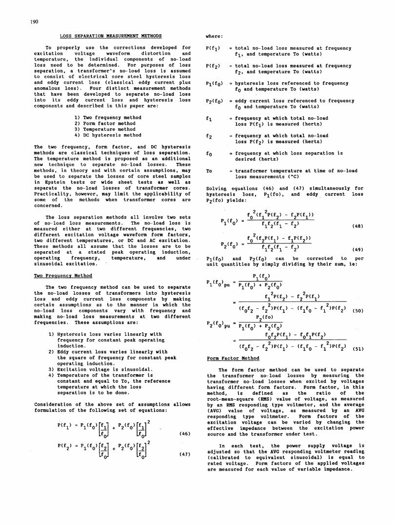
LOSS SEPARATION MEASUREMENT METHODS

To properly use the corrections developed forexcitation voltage waveform distortion andtemperature, the individual components of no-loadloss need to be determined. For purposes of lossseparation, a transformer's no-load loss is assumedto consist of electrical core steel hysteresis lossand eddy current loss (classical eddy current plusanomalous loss). Four distinct measurement methodsthat have been developed to separate no-load lossinto its eddy current loss and hysteresis losscomponents and described in this paper are:

1) Two frequency method2) Form factor method3) Temperature method4) DC hysteresis method

The two frequency, form factor, and DC hysteresismethods are classical techniques of loss separation.The temperature method is proposed as an additionalnew technique to separate no-load losses. Thesemethods, in theory and with certain assumptions, may

be used to separate the losses of core steel samplesin Epstein tests or wide sheet tests as well as

separate the no-load losses of transformer cores.

Practicality, however, may limit the applicability ofsome of the methods when transformer cores are

concerned.

The loss separation methods all involve two setsof no-load loss measurements. The no--load loss ismeasured either at two different frequencies, twodifferent excitation voltage waveform form factors,two different temperatures, or DC and AC excitation.These methods all assume that the losses are to beseparated at a stated peak operating induction,operating frequency, temperature, and undersinusoidal excitation.

Two Frequency Method

The two frequency method can be used to separatethe no-load losses of transformers into hysteresisloss and eddy current loss components by makingcertain assumptions as to the manner in which theno-load loss components vary with frequency andmaking no-load loss measurements at two differentfrequencies. These assumptions are:

1) Hysteresis loss varies linearly withfrequency for constant peak operatinginduction.

2) Eddy current loss varies linearly withthe square of frequency for constant peakoperating induction.

3) Excitation voltage is sinusoidal.4) Temperature of the transformer is

constant and equal to To, the referencetemperature at which the lossseparation is to be done.

Consideration of the above set of assumptions allowsformulation of the following set of equations:

p(f1 p1(f0 [fI 2 f0 f

f1 f+ (46)

f f] (47)

P(f1) = total no-load loss measured at frequencyfl, and temperature To (watts)

P(f2) = total no-load loss measured at frequencyf2, and temperature To (watts)

PI(fo) = hysteresis loss referenced to frequencyfo and temperature To (watts)

P2(fO) = eddy current loss referenced to frequencyfo and temperature To (watts)

fi. = frequency at which total no-loadloss P(fl) is measured (hertz)

f2 =- frequency at which total no-loadloss P(f2) is measured (hertz)

fo = frequency at which loss separation isdesired (hertz)

To = transformer temperature at time of no-loadloss measurements (°C)

Solving equations (46) and (47) simultaneously forhysteresis loss, Pl(fo), and eddy current lossP2(fo) yields:

P (f0)

f 2(f P(f ) - f P(f ))0 1 2 2 1

f1f2 1 f2)2

f0 (f2P(f f1P(f2 ))

2(f0° f,.f2(f - f )1 2 1 2

(48)

(49)

P1(fo) and P2(fO) can be corrected to perunit quantities by simply dividing by their sum, ie:

P_ (f0)1 0 pu P (f0) + P2(f0

2

f 2P(f ) f2 P(f)1 2 2 1

(ff -f2 )f ) (ff )P(ff0 2 2 1 1 0 1 2 (50)

P2(fo)2 0 pu P (f + P(f01~I0 2 0

f f2P(f) f0fIP(f2)

)fPfff2 Mf (f f - f 2P(f)0 2 2 1 1 0 1 2 (51)

Form Factor Method

The form factor method can be used to separatethe transformer no-load losses by measuring thetransformer no--load losses when excited by voltageshaving different form factors. Form factor, in thismethod, is defined as the ratio of theroot-mean-square (RMS) value of voltage, as measuredby an RMS responding type voltmeter, and the average(AVG) value of voltage, as measured by an AVGresponding type voltmeter. Form factors of theexcitation voltage can be varied by changing theeffective impedance between the excitation powersource and the transformer under test.

In each test, the power supply voltage isadjusted so that the AVG responding voltmeter reading(calibrated to equivalent sinusoidal) is equal torated voltage. Form factors of the applied voltagesare measured for each value of variable impedance.

190

where:

The assumptions used in the form factor methodare:

1) Hysteresis los's is independent of-excitationvoltage waveform if the voltage waveformcontains no more than its normal number ofzero values pet cycle.

2) Eddy current loss is assumed to vary with thesquare of the RMS responding voltmeterreadings..

3) The fundamental frequency, fo, of theexcitation voltage and core temperature, To,

remain constant.4) Peak operating induction is maintained

constant.

4) The temperature coefficient of core steelelectrical resistivity, vL (l/C), is knownit 20°C.

5) Peak operating induction,remains constant.

Based on theequations become

P(T ) = P +1 1

P(T2) = P +

where:

above assumptions the resulting(reference equation-(35)):

P2To) (1/v To 20)

1

P '(To) (1/cs + -To -,20)2 (1/a + T2-20)

(58)

(59)

From these assumptions the following set of equatcan be written:

P(kl) = P1 + k1P2

P(k2) = P1 + k2P2

where:

P(kM) = total no-load loss measured with an RHSvalue of excitation voltage VRMS1 (watts)

P(k2) - total no-load loss measured with an RMSvalue of excitation voltage VRMS2 (watts)

kl = square of the form factor when P(kl) ismeasured /

k2 = square of the form factor when P(k2) ismeasured

P1 hysteresis loss component (watts)

P2 eddy current loss under sinusoidalexcitation (watts)-

Solving equations (52) and (53) simultaneouslyP1 and P2 gives:

kP(k) - kP(k1 2

1i k -k2 1

P(k2) -P(k

2 k -k2 1

In terms of per unit quantities the hysteresisPlpu, and the eddy current loss, P2pu' are:

1

lpu= P1- + = (k-

iP2 2

p2pu P + P2 (k2

Temperature Method

k2 1 1. 2

l)P(k )-(k - 1)P(k2)P(k ) P(k )- 2 1

l)P(k ) (k, l)P(k2)

ions P(T1) = total no-ioad loss measured at core

temperature T1 (watts)

(52) P(T2) = total no-load loss measured at core

temperature T2 (watts)-

= temperature coefficient of resistivity (1/C)

= core temperature when P(T1) is measured (IC)

To = reference temperature at which P1 and P2are to be determined (IC)

P1 = hysteresis loss component (watts)

P2(To) = eddy current loss component at referencetemperature To (watts)

Solving equations (58) and (59) simultaneously forhysteresis, loss, P1, and eddy current loss,P2(To), yields:

for

(54)

(55)

loss,

(1/* + To - 20) P(T

(l/ + T - 20) 2

p = 1I (I/v + To - 20)

(1/v + T1 - 20)

P(T ) -

2( ) (1/ + To - 20)(1/cs + T1 - 20)

(1/J + To - 20)(1/as+ T2 - 20-) (Tl)(1/cs + To - 20)(1/v - T - 20)2

P(T2 )(1/c + To - 20)(1/v + T2 - 20)

Converting the hysteresis loss, Pl, andcurrent loss, P2(To), to per unit gives:

P1 P o

plpu P1 + P2(To)

1 2

(60)

(61)

the eddy

(l/c + To -0) PT ) (l/ + To - 20)P(T( /oL + T -20) 2 (l/a + T2 - 20) 1

(56) F - l c T 1P(T )- ( / s T -20) P(T((1/ + To 20) 1 (l/ + Ti - 20) 2

(62)

(57)

The third method that can be used for losiseparation involves measuring the no-load losses of atransformer when the transformer's core is atdifferent temperatures. The assumptions used in thetemperature method are:

1) Hysteresis loss is inidependent of temperature2) Core steel electrical resistivity increases

linearly with temperatures.3) Eddy current loss varies inversely with

electrical resistivity.

P

p2pu P1 + P(TO)2

P(T ) - P(T2

(i/t+ o 2

P(T) 1/cs+ To'-20) P(T)[_lc+T - [1 (l/c + T - 20) 2

6 )O(63).

DC Hysteresis- Method

:Loss separation can also be accomplished bymeasuring the hysteresis loss component directly fromhysteresis loop data. The hysteresis loop, as shownin Figure 2, is formed by exciting the core at verylow frequency, approaching DC, so that virtually noeddy currents are generated to produce extra loss.

191

Ti

192

As shown previously the net energy delivered to thematerial per unit volume is identically equal to thearea contained within the hysteresis loop for onetraverse of that loop. To calculate the hysteresisloss for AC excitation the volume of the corematerial, V, must be known as well as the frequency,fO, at which the loss separation is to be done. TheAC excitation peak operating induction must match themaximum induction of the DC hysteresis loop tomaintain equivalent loss per cycle.

Therefore, the AC hysteresis loss can becalculated from the hysteresis loop data as:

PI = ABH V f0 (64)

where:

ABH - area contained within DC hysteresis loop(joules/meter3)

V = core volume (meter3)

fo= AC excitation frequency (hertz)

PI = hysteresis loss component (watts)

To determine the eddy current loss component, P2,

the no-load losses are measured at frequency, fo,and at the stated peak operating induction. The eddycurrent component is then simply the differencebetween the measured no-load losses and thehysteresis loss as measured from hysteresis ioopdata, that is,

P2 = P -- PI (65)

where:

P = total no-load losses measured (watts)

PI = hysteresis loss component (watts)

P2 = eddy current loss component (watts)

Conversion to per unit is simply:

P

lpu P

pp -=2pu P

(66)

(67)

CONCLUSIONS

1) Accurate measurement of no--load losses of

distribution transformers is important because of

the economic value associated with these losses.

*t

2) The measured no-load losses are subject to errors

produced by excitation waveform distortion and

temperature.

3) Methods developed for converting -the no-loadlosses measured under non-sinusoidal excitationcondition to sinusoidal excitation cinditions are

reviewed. Much of the experimental data has been

developed using Epstein sample.. In such tests,the flux density is relatively uniform.

4) Loss measurements at different temperatures on

both Epstein samples and completed transformercores show that the losses decrease with

increasing temperature. This loss decrease, can

be attributed to decreasing eddy current loss as

the core steel's electrical resistivity increaseswith increasing temperature.

5) A general method for correcting no-load lossesmeasured at any temperature and with distortedexcitation voltage to standard conditions ofreference temperature and sinusoidal excitationis developed.

6) Four methods to separate the no-load losses intohysteresis and eddy current loss components aredescribed.

7) The flux density in a completed transformer coreis not uniform. In general, even though theexcitation voltage may be purely sinusoidal,there are natural harmonic fluxes in the core.The effect of this flux condition on the ratio ofhysteresis and eddy current losses needs to beinvestigated. This ratio is used in the methodfor. correcting the measured losses to standardreference conditions.

8) Since the temperature correction method alsorequires knowledge of, the ratio of hysteresis andeddy current loss, the effect of non-uniform fluxdensity, and natural flux harmonics on thetemperature variations of losses needs to beinvestigated.

9) The various methods -of loss separation should becompared against each other to confirm thevalidity of the assumptions involved.

ACKNOWLEDGEMENTS

The authors would like to thank K. Foster for useof his unpublished data regarding loss separationtemperature dependency and D. Whitley for use of hisdata regarding transformer no-load loss temperaturedependency.

The authors would also like to thank theUniversity of Missouri Student Trainees, Greg Vetterand David Kilp, for preparation of the figures usedin the paper, and thank Marilynn Zuck and PamelaPropst for the typing of the manuscript.

REFERENCES

F. E. Werner, "Electrical,Steels: 1970-1990",Proc. of Sym. Energy Efficient ElectricalSteel, TMS of AIME, 1980, pp. 1-32.

121(]S. Austen Stigant and A. C. Franklin, "J & PTransformer Book", 10th Edition.

1T. R. Specht, L. R. Rademacher and H. R. Moore"Measurement of Iron and Copper Losses inTransformers", AIEE Trans., Aug. 1958, pp.470-476.

141- J. W. Shilling,.and G. L. Houze Jr., "HagneticProperties and Domain. Structure inGrain-Oriented 3? Si-Fe", IEEE Trans. onMagnetics, Vol. 10, No. 2, June 1974, pp.195-223.

C. A. Holt, "tntroduction to ElectromagneticFields and Waves", John Wiley & Sons, 1963.

[61H. Cotton, "Electrical Technology", Book, Sir

Isaac Pitman & Sons, Ltd. (6th Edition).

KJ. Overshott, "The Use of Domain Observationsin Understanding and Improving MagneticProperties of Transformer Steels", IEEETrans. Hag. Vol. 12, 1976, pp. 840-845.

[81K. J. Overshott, "The Causes of the Anomalous Lossin Amorphous Ribbon Materials", IEEE Trans.Hag., Vol. 17, No. 6, Nov. 1981, pp.2698-2700.

[9]A. Asner, "Transformer No-Load Losses with

Distorted Voltage Waves", The Brown BoveriReview, Vol. 47, No. 12, Dec. 60, pp.875-882.

J. McFarlane and M. J. Harris, "The Control ofFlux Waveforms in Iron Testing By theApplication of Feedback AmplifierTechniques", Proc. IEE, Vol. 105A, 1958, pp.395-402.

T. Nakata, Y. Ishihara, M. Nakano, "Iron Losses ofSilicon Steel Core Produced by DistortedFlux", Elec. Engr. in Japan, Vol. 90, No. 1,1970, pp. 10-20.

[121J. D. Lavers and P. P. Biringer, "Prediction of

Core Losses for High Flux Densities andDistorted Flux Waveforms", Magnetics Conf.,

-- June 1976.

R. A. Newbury, "Prediction of Loss in SiliconSteel from Distorted Waveforms", IEEE Trans.on Hagnetics, Vol. Mag-14, No. 4, July 1978,pp. 263-268.

K. Foster, "Temperature Dependence of LossSeparation Measurements for Oriented SiliconSteels", (To Be Published).

Discussion

Ramsis S. Girgis, (Westinghouse Electric Corporation, Pittsburgh, PA):This discusser would like to point out that formula 24, which is present-ly used in the standards, is sufficiently accurate when appropriate valuesof Pl and P2 are used. It provides almost the same value of wave-formcorrections as Eq. 23 for typical ratios of VAVG VRMS, 0.95 <VAVG/VRMS) < 1.05, because

V V

[P +P )]2 [ )21 2 VAVG 1 2 ( RMS

Normally, temperature is expected to have a greater effect on iron lossesof thicker steels, e.g., 12 mil in comparison to 9 mil steel. Were cores

193

used to obtain data of Fig. 7 heated in an oven? Would the authors com-ment on the effect of temperature distribution in relation to the resultsof Fig. 7. The figure demonstrates a larger effect of temperature on ironlosses of thinner steels.

This discusser thinks that the factor developed in the paper to accountfor the effect of temperature is fairly complex while it does not accountfor many important considerations that determine that effect in an ac-tual tranformer. The source of complexity in the factor developed is theconsideration of effect of termperature on Pl and P2, which is not ofprime significance. Most appropriate values of Pl and P2 themselvesare a subject for debate. A paper authored by this discusser (plannedfor presentation at the Winter Power Meeting in 1985) will include a sug-gested factor for effect of temperature on core losses based on actualtest values of commercial transformers.

Finally, it is to be noted that the relative error-column in Table I in-cludes values that are between 10 to 80 percent of the total effect oftemperature. Would the authors please comment on the difference inthe heating process and magnetic flux distribution between an actualtransformer core and an Epstein sample relative to the applicability ofthe results of Table I to commercial cores.

Manuscript received May 31, 1984.

R. L. Boggavarapu and D. S. Takach: The authors wish to thank Dr.Girgis for his comments.

No-load losses in core-coil assemblies of distribution transformers weremeasured while they were heated in an oven. A thermocouple was tapedto one of the core legs. The core and oven temperatures were recordedby a chart recorder. The core-coil assembly was left in the oven for about24 hours after the temperatures had stabilized. The oven door was openedfor making the connections for the test and closed immediately.* Testswere conducted while the oven was still operating. The difference intemperature, before and after the test, was observed to be less than 1 'C.No-load losses of core-coil assemblies of 10 thru 50 Kva for cores madeof different thicknesses of steel were measured. The ratio of no-load lessat 85°C to that of 20°C varied from 0.937 to 0.954 in these units.The ratio of hysteresis to eddy-current losses, for a given material,

is a complex function of many parameters such as temperature, frequencyand maximum flux density. Any method of correcting the no-load lossfor effects of temperature and waveform distortion would requireknowledge of this ratio. Test data were provided which showed how theselosses vary with temperature. A correction factor was developed by theauthors for the general case when the three temperatures, (i) at whichthis ratio was known, (ii) at which the no-load loss was measured, and(iii) which the loss has to be corrected to, are different. Under specialtest conditions or with further simplifying assumptions, this factor couldbe made simpler.However, agreement is yet to be reached whether thecorrection, to the measured no-load loss, is to be made by the manufac-turer or the user. The authors would welcome additional test data andcontents.

Manuscript received September 7, 1984.

*A line conditioner was used to control the waveform of the applied voltage.