Computational Statistics (2005) 20:503-519 �9 Physica-Verlag 2005

Improving Estimation in Speckled Imagery

Klaus L. P. Vasconcel los 1, A l e j a n d r o C. F r e r y 2, L u c i a n o B. Silva a

1 U F P E - C C E N , D e p a r t a m e n t o de Es t a t i s t i c a , C i d a d e Univer -

s i ts 50740-540 Recife, P E - Braz i l 2 UFAL, D e p a r t a m e n t o de Tecno log i a da Informa~go, B R 104

N o r t e k m 97, 57072-970 Macei6 , AL - Braz i l 3 U n i v e r s i d a d e Sa lgado de Ol ivei ra , Av. M a s c a r e n h a s de M o r a e s

1919, 50740-540 Recife, P E - Braz i l

Summary

We propose an analytical bias correction for the maximum likelihood esti- mators of the G o distribution. This distribution is a very powerful tool for speckled imagery analysis, since it is capable of describing a wide range of target roughness. We compare the performance of the corrected estimators with the corresponding original version using Monte Carlo simulation. This second-order bias correction leads to estimators which are better from both the bias and mean square error criteria.

Keywords : Bias Correction, G ~ distribution, Image Analysis, Maximum Likelihood, Speckle Noise.

504

1 I n t r o d u c t i o n

The aim of this paper is to compare the performance, in terms of bias, of four different estimators for the homogeneity parameter of a distribution that proves to be very useful in modelling image data contaminated by speckle noise, as SAR (Synthetic Aperture Radar), sonar, ultrasound-B and laser imagery. Those data are generated by systems that employ coherent illu- mination, which generate a stochastic multiplicative noise along with the information. The statistical properties of this noise have been extensively studied in the last thirty years (see Goodman 1976, Oliver &= Quegan 1998).

Most of the proposed models for image data can be considered as variations of a generM framework, the multiplicative model. The multiplicative model assumes the resulting image to be the product of two statistically indepen- dent random variables which are related, respectively, to the target informa- tion and the speckle noise. Within this framework, a particularly sucessful distribution that was proposed as a model for data coming from images of extremely heterogeneous regions (e.g., urban areas in SAR imagery) is that one called the G7 distribution. This distribution was introduced by Frery, Mtiller, Yanasse & Sant 'Anna (1997a) and practical applications have shown its outstanding performance in fitting that type of data. (for an application to statistical classification see Mejail, Jacobo-Berlles, Frery & Bustos 2003). Recent results propose it as a universal model for speckled data (see Mejail, Frery, Jacobo-Berlles & Bustos 2001). Robust procedures have been also studied for particular cases of this law (see Frery, Sant'Anna, Mascarenhas & Bustos 1997b, Bustos, Lucini & Frery 2002), and improved inference using resampling is presented in Cribari-Neto, Frery & Silva (2002).

The ~ distribution is indexed by two parameters; one is directly associated with the degree of homogeneity of the image under study, the other being a scale parameter. Because of this association, good estimation of the first parameter, the homogeneity parameter, is very important, in particular, for classification procedures, where we need to discriminate different data sets according to the degree of homogeneity of the imaged area. It is then crucial to devise estimators of the parameters that present good performance in terms of bias from the available data.

This paper discusses estimation of the homogeneity parameter of the C ~ dis- tribution, using four possible alternatives: an estimator based on the method of moments, a quantile estimator, the maximum likelihood estimator and its bias corrected version. In particular, analytic bias correction has proved being useful in practical situations as shown, for instance, in the works by Pike, Hill & Smith (1980), Young & Bakir (1987) and Cordeiro & Vasconcellos (1999). We also present simulations that assess the extent of the bias reduction of each estimator, for different values of the homogeneity parameter.

505

The first proposal we consider is to es t imate the homogenei ty pa ramete r by equat ing the moments of the d is t r ibut ion to the sample moments . However, the moments of the G ~ d is t r ibut ion may be infinite, according to the t rue value of the homogenei ty parameter , which, of course, is unknown. There- fore, the t radicional me thod of moments can only be used if we assume the homogenei ty pa ramete r to belong to a res t r ic ted interval. This const i tu tes a l imitat ion in the use of the classical me thod of moments approach.

An a l ternat ive to the first proposal is a quanti le es t imator . Since the moments of the dis t r ibut ion can possibly be infinite, we also considered a quant i le es t imator , obta ined by equat ing some quanti les of the d is t r ibut ion to the sample quantiles. For example, we can equate the median of the d is t r ibut ion to the sample median and equate the difference between the first and th i rd quanti les of the dis t r ibut ion to the respective sample inter-quant i le range. The problem with this quanti le method is tha t the d is t r ibut ion function we are dealing with does not have a closed-form expression and the es t imators have to be found, in practice, through numerical inversion of complicated integrals.

A thi rd possible approach is maximum likelihood. The difficulty, however, is tha t the ext reme points of the l ikelihood function for G o da t a do not have a closed analyt ical form. Maximum likelihood est imates for this d is t r ibut ion are to be found, in practice, by the use of numerical maximiza t ion routines. The likelihood function is, in many cases, very flat, which can br ing numerical problems when we try to maximize it with respect to the pa ramete r s (see Frery, Crihar i -Neto & Souza in press).

Finally, since our main interest lies in obtaining es t imators wi th good bias performance, we can also consider a bias corrected est imator . We know the maximum likelihood es t imator to be, in general, a biased es t imator of the t rue pa ramete r value. If b(ON) is the bias E[ON -- 0] of the max imum likelihood

es t imator ON of a pa ramete r 0 from a sample of size N, then, typically, we have

b(~) = B(O) + O(N_2)" N

The term B(O)/N is commonly called the second-order bias. The idea of bias

correction is, then, to consider the a l ternat ive es t imator ~N = ~ n - - B(~N)/N, which is expected to correct the bias of the original max imum likelihood es- t imator . In fact,, it can be shown tha t E[~N -- ~] ---- O(N-2), which confirms tha t this last es t imator provides a bias reduction of the former. This bias reduct ion scheme has been used in the l i tera ture in many different si tua- tions. Cox & Snell (1968) obta in a very general formula to calculate the second-order bias of the maximum likelihood es t imators for the case of in- dependent observations. F i r th (1993) introduces an es t imator tha t reduces bias, obta ined as the solution of a modified score equation. More recently, Cribar i -Neto & Vasconcellos (2002) compare different bias reduct ion meth-

506

ods for the maximum likelihood estimators of the parameters of the beta distribution.

The rest of the paper has the following structure. In Section 2, we introduce the G ~ distribution. In Section 3, we briefly discuss the techniques proposed to estimate the parameters of the distribution. In Section 4, we present simulation results, which allow us to compare the performances in terms of bias of the estimators discussed. Finally, in Section 5, we summarize the main results of this study.

2 T h e G ~ d i s t r i b u t i o n

Speckled imagery suffers from a contamination that can be succesfully de- scribed by what is called the Multiplicative Model. This model can be applied to any type of signal that employs coherent illumination, as is the case of ul- t rasound B-scan imagery, sonar signal, laser and synthetic aperture radar (SAR) data.

The Multiplicative Model postulates that the observed value in each res- olution cell is the result of many contributions from elementary reflectors (scatterers). Since the illumination is coherent and, therefore, the phase of the original signal is recorded, the return can be modelled by the complex number

A = e x p ( i r

J

where i = ~ - T and Aj(w) is the observed amplitude returned by the J- th reflector, which is at observed phase ~j(w). If the number of scatterers becomes infinitely large (j --~ oo), with no amplitude dominating over the others (maxjVar(Aj)/y~kVar(Ak) -~ 0) and if the phases have uniform distribution (Oj ~ U(-Tr, ~r]), all random variables being independent, then, from Central Limit Theorem, the distribution of A will be Complex Gaussian.

The Complex Gaussian distribution was extensively studied by Goodman (1963), and the main result for our purposes is that, when A obeys this law, the intensity IA] 2, observed for each resolution cell, follows an exponential distribution with mean cr > 0, a being called the mean cross section. There- fore, a good model for the observations is Z = aY, where Y is an exponential random variable with unit mean. An extension of this model, where we allow cr to be random, leads to the general form of the Multiplicative Model, also known as Product Model, for the return.

Identifiable targets are, therefore, seen as outcomes of exponentially dis- tr ibuted random variables with different means. Since it is quite hard to separate observations under this assumption, multilook processing is applied to data. A simplified version of this technique consists of taking the mean of

507

L independent observations of the same object having, thus,

z ( L ) : 1 L L -s E Zt = O-L E Ye = aY(L).

~=1 ~=1

(i)

Hence, the noise y(L) follows a F (L ,L) distribution with L > 1, and the bigger the value of L, the easier the discrimination among different targets. The density of y(L) is

L L fy(cl (y) = ~--'7"TX,~y L-! e x p ( - L y ) , y > 0.

t [L)

Constant mean cross section target classification requires discrimination am- ong outcomes of F(L, Lac 1) random variables, the mean cross section ac > 0 being different for each class c. The number of looks L is an integer number which is considered as known or estimated beforehand, and it is constant for the whole image.

The hypothesis of constant mean cross section is valid for extended homo- geneous targets, for which speckle noise is fully developed. This happens mostly when the wavelength is bigger than the mean roughness. This, for instance, is the case of agricultural fields, grass and deforested (cut and /or burnt) flat areas in SAR imagery. When roughness has the same order of the wavelength, cr requires a stochastic modeling since it varies within the class from pixel to pixel. The mean cross section can be assumed independent of the speckle noise.

Several stochastic models have been proposed for varying cr but, in order to be successful, a model has to lead to distributions that explain real da ta and that are also tractable. One of the most succesful models is the G a m m a mean cross section, i.e. a ~ P(a, A), which leads to the K(ch ,~, L) distribution. The density for the return is given in this case by

f z ( z ) = 2(ALz)~+L r ( L ) r ( ~ ) ' (2)

with z, a, A > 0 and L > 1, where K~ is the modified Bessel function of the third kind and order u (see Gradshteyn & Ryzhik 1980) This model explains heterogeneous data tha t the F(L, La -1) law for the return fails to fit.

The main advantage of the K distribution, apart from its capability of ex- plaining data, is that the parameter a has a concrete interpretable meaning: it measures the homogeneity of the target, in the sense that big values of (c~ > 15, ibr instance) can be associated to homogeneous areas, while small values are usually observed in heterogeneous areas.

However, the K(a , A, L) distribution is hard to deal with, since its cumula- tive distribution function can only be written (in recursive form) by making

508

restrictions on the parameter space. Furthermore, dependable implementa- tions of the function K v ( x ) are available only for relatively small ranges of and x. Also, it fails to fit observations from extremely heterogeneous regions such us urban spots and forests over undulated relief. Searching for a model capable of describing also this type of data, Prery et al. (1997a) proposed a reciprocal of Gamma law for the mean cross section.

Still within the Multiplicative Model framework, this proposal models the random variable a using the distribution characterized by the density

X c~

f ~ ( x ) -- 7~r(_---- ~ exp(--"/x-1), (3)

where - a , % x > 0, named inverse gamma. We use the notation a F -1 (a ,7 ) . The name stems from the fact that if c~ ,-~ F - l (a , -y) , then ~-1 ,.~ F ( - a , V). This assumption for a leads to the C ~ model for the return, which is characterized by the density

L L F ( L - oe) z L

f z ( z ) = ~-r( -a) r (L) (~ + zL)L-~' (4)

where - a , 7, z > 0 and L > 1. We use the notation Z ~ G~ 7, L).

The heavy-tailedness of the G ~ model is assessed in Figure 1: where the densities G~ 4, 2), F(1, 1) and Gaussian, all three with mean and variance set to one, are shown. Though these laws have the same mean and variance, their behaviours for large values of z are quite different.

The distributions characterized by eqs. (2) and (4) are closely related be- cause the F and F -1 distributions are both particular cases of a more general distribution, known as the Generalized Inverse Gaussian distribution, exten- sively studied in Jcrgensen (1982) and Seshadri (1993). This relationship leads to similar interpretations of the parameters a and - a of the K and G O distributions, respectively (see Frery et al. 1997a).

The moments of a G/~ % L)-distributed random variable are given by

{ (~)~ r(-~-~)rIL+~/ E (Z ~') = r(-a)r(L) if a < - r

oo if - r < _ a < O '

with L > 1.

The Qo law achieves its goal, since it is able to describe extremely heteroge- neous data. (such as those coming from urban spots in SAR imagery) that were left unexplained by the K model. It has also proved being quite flexible and capable of describing heterogeneous observations that were well described by the K distribution, as well as homogeneous targets whose "natural" model is the F law. This, combined with the fact that the numerical and analytical

509

10 o

10 -1

10-2

:~ 10-,5 c

10 - 4

10-5

10-6 0

. . . . i . . . . i . . . . i '

I0

z

i , , l l

15 20

Figure 1: Densities of the G~ 4, 2), F(1, 1) and N 0 , 1) distributions (solid, dots, dashes, respectively), in semilogarithmic scale.

properties of the G o distribution are simpler than those of the K law, led to the proposal of tha t distr ibution as a universal model for speckled da ta (see Mejail, Jacobo-Berlles, Frery & Bustos 2000, Mejail et al. 200t). The com- putat ion of the cumulat ive distribution function of a G~ 7, L)-distr ibuted random variable is immediate using the relationship that can be seen in Me- jail et al. (2001):

P r ( Z < t) : T2L,_2a(-at/v), (5)

where Tn,~ is the cumulative distribution function of an F-dis t r ibuted ran- dora variable with 77 and ~; degrees of freedom. Since the F distribution is commonplace in statistical software, there are plenty of dependable routines (and tables, also) tha t provide these values.

3 P a r a m e t e r E s t i m a t i o n

From the previous section, it is seen that the moments of the G0 distribution can be infinite, depending on the values of c~. Therefore, the method of moments can only be used if we assume beforehand tha t the homogeneity paramete r belongs to a specific proper subset of ( -oo , 0).

For example, suppose tha t c~ C ( - o o , - 1 ) . In this case, the parameters of the distribution can be estimated, for example, by equating the theoretical values

510

of E(Z) and E(Z 1/2) to the corresponding sample moments. If ;~ and ~ / 2 are the sample moments, it is not difficult to see that c~ can be estimated as the root of the nonlinear equation

V/-Z--~-Z-~F(-c~- 1/2) ~ #I /2F(L) F ( - a ) = V ~-~ r -~-~-~ /2) (6)

The complicated nonlinear equation above can only be solved through nu- merical methods. The estimator defined by its root also only makes sense if we suppose that c~ < -1 . The method of moments seems, therefore, to be quite problematic to solve our specific estimation problem.

Assuming other restrictions for c~ in ( -oo , 0), other systems of moment equa- tions can be formed.

A second alternative consists of using qua.ntile estimators. Let m be the sample median, while ql and q3 represent, respectively, the first and third sample quartiles. We can estimate c~ and "7 by solving the nonlinear system defined by

f0 TM j~qq~ 1 J'z(z)dz = 2 ' and f z ( z )dz = ~, (7) 1

where f z ( z ) is the density presented in equation (4). Although this esti- mation method does not need any assumption about the true value of a, it requires the numerical solution of a nonlinear system involving two compli- cated numerical integrals.

If the system presented in equations (7) is to be solved, we recommend the use of a software platform that provides reliable routines to obtain numeri- cally the cumulative distribution function Tv, ~ of an F-distr ibuted random variable with r l and a degrees of freedom, since the system can be rewritten a s

T~L,_~s(-amp?) = 1/2 (s)

T2L,-2a(--aqa/'@) -- T:L,-2S(--aql/'@) = 1/2. (9)

A third alternative is maximum likelihood. Prom the previous section, it can be readily seen that, for a sample X 1 , . . . , XN of N independent obser- vations, all with the same G~ % L) distribution, where L is known, the log-likelihood flmction is

L - 1 N

~(c~, ~/) = N ~ log(r - c~) - N ~ log('y) - (L - c~) ~ log(~/+ LXi). r = 0 i = 1

(10)

This function, as we know, must be maximized with respect to c~ and 3' in order to obtain the maximum likelihood estimators. Differentiating the

511

previous equation with respect to ~ and % and equat ing these derivatives to zero, we obta in the nonlinear system

{ ~ = 0 (~' - ~ ) - ~ - ~ ~ = ~ log 1 + = o

= o .

Since the log-likelihood is unbounded from below and its derivatives are con- t inuous functions, then, if the solution of the above system exists and is unique, it will correspond to the max imum likelihood es t imator of the pa- rameters. We suppose here tha t this is the case and the max imum likelihood es t imates (MLE in the following) will correspond to the point of null gradient of the log-likelihood function. The main difficulty here is tha t we cannot ex- press the max imum likelihood es t imates analyt ica l ly in terms of the sample values; in fact, we even do not have a proper sufficient set of s ta t is t ics for the parameters . The only way of obta ining the max imum likelihood es t imates is, again, by solving numerical ly the equations. Another difficulty lies in the fact tha t the likelihood function to be maximized can become very flat in some si tuat ions and this can bring numerical problems in a numerical op t imiza t ion routine.

Finally, we will also consider the second-order bias corrected es t imator briefly presented in Section 1. This bias correction can be obta ined from expected values of second and th i rd order derivatives of the log-likelihood function, as follows.

Let Us and U~ denote the derivatives of the log-likelihood with respect to c~ and 3', respectively. Similarly, we represent the higher order derivatives as U ~ = 02~/Oc~ ~, U ~ = 02g/0c~03", U.y~ = 02g/072, U ~ = Oag/Oa207 and so on. The s t anda rd nota t ion commonly used for the following moments i s ~ = E[U~] , ~ = Z[U~] , ~ = E [ U ~ ] , ~ , ~ = E[U~U~], ~ = E[U~] , ~ , ~ = E[U~U~.y] and so on. Also, the derivatives of the mo-

ments with respect to the parameters are denoted as n ~ ) = 0 n ~ / 0 ~ y , n(~y) = 0~-y/0c~ etc. In par t icular , we note tha t n~,~, ~ , - r and ~-y,~y are the entries of the Fisher information mat r ix for the parameters ~ and % As we know, its inverse gives the large-sample covariance mat r ix of the max imum likelihood est imators. We denote the entries of this inverse by ~a,~, n~,-y and n~,w.

The second-order bias of the maximum likelihood es t imator & of ~ is, ac- cording to Cox & Snell (1968), given by the expression

B(&) _ ~ ~,~ns,t n(~ _ ~e~st (11) N r.s,t,

where the sum is over the eight possible combinat ions for (r, s , t ) . In the following we obta in the necessary quant i t ies for the problem at hand.

512

The derivatives of second and third-order of the log-likelihood in (10) are

U ~ = - - N V ' L - I ( -- a) -2, Ua.y _- _ g + EN:I(.7_ + L X i ) - I ,

U~.y= 7--~-+N~ ( L _ ~ ) y~N=I(7 + LX{ ) -2 U~a:_2g~r=o(r_a)-3L-1

: o , : 5

Uv~ _ 2ga ~ = 1 ( ' 7 + LXi ) -3" - - - 7 - - ~ - 2 ( L - a ) g

Taking expected values in the expression above, we obtain the following re- sults:

],;a,a ~ - - "~(L-a)(L-a+l) : -- _ . . ~ I ' ; a ' 7 : g ( ~ ) N '

~ = "Y2(L-~)2(L-~+I) E2jr -~ g ( c ~ ) L N

L - 1 ~aaa = - 2 N ~-~-~=o (r - a) -8, ~a~7 = 0, L N ( L - 2 a + I ) 2 c ~ L N ( L - 2 a + 3 )

t~ay. I = 72(L_a)(L_a+l), ~/7~/ ~- --T3(L_aTl)(L_c~+2)~

~(~) ~(~) = O, O~Ct ~-- ]~uOlOlOt , I~C~Ot

where g(a) - a ( L - a ) : L-1 = ~ = o (r - a) -2 - L (L - a + 1). From the results above and equation (11), we obtain the expression for the second-order bias of 6:

B(&) 1 (L - a ) ( A a 6 + B a 5 + C a 4 + D a 3 + E a 2 + F a + G) - , ( 1 2 )

N 2 (L - a + 2)g2(a)N

where

A = 2 S 3 , B = - ( S L + 4 ) S 3 , C = ( L + l ) ( 1 2 L S 3 + S 2 ) ,

D = -8L3S3 - 3L 2 (4S3 + $2) + L (2 - 3S2),

E : 2L4S3 + L 3 (4S3 + 3S2) - 3L 2 (2 - $2) - 8L

F = - L 4 S 2 + L 3 ( 6 - $ 2 ) + 1 4 L 2 + 8 L , G = - 2 L 4 - 6 L 3 - 4 L 2,

L - 1 with Si = Y~r=0 (r - a ) - i .

In order to assess the relevance of improving the MLE estimator of a with respect to its bias, Figure 2 shows the plot of equation (12) for L = 1. The range of this plot depict practical situations: a stems from - 4 to -0 .5 , the sample sizes (N E {49, 81,121,169}) corresponds to squared windows of sides 7, 9, 11 and 13, respectively, which are usual sample sizes in image processing techniques.

513

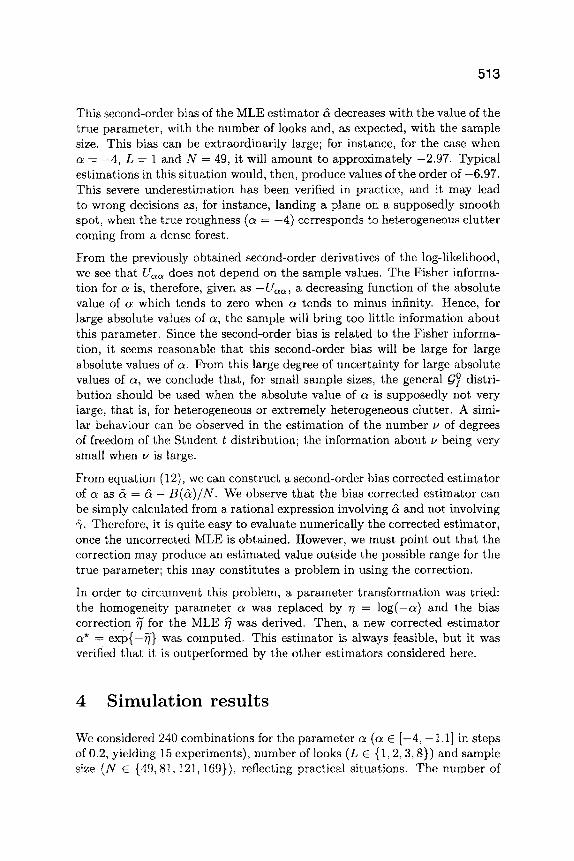
This second-order bias of the MLE estimator 5 decreases with the value of the true parameter, with the number of looks and, as expected, with the sample size. This bias can be extraordinarily large; for instance, for the case when a = -4 , L = 1 and N = 49, it will amount to approximately -2.97. Typical estimations in this situation would, then, produce values of the order of -6 .97. This severe underestimation has been verified in practice, and it may lead to wrong decisions as, for instance, landing a plane on a supposedly smooth spot, when the true roughness (v~ = - 4 ) corresponds to heterogeneous clutter coming from a dense forest.

From the previously obtained second-order derivatives of the log-likelihood, we see that U ~ does not depend on the sample values. The Fisher informa- tion for (~ is, therefore, given as - U a a , a decreasing function of the absolute value of a which tends to zero when a tends to minus infinity. Hence, for large absolute values of a, the sample will bring too little information about this parameter. Since the second-order bias is related to the Fisher informa- tion, it seems reasonable that this second-order bias will be large for large absolute values of (~. From this large degree of uncertainty for large absolute values of a, we conclude that, for small sample sizes, the general G O distri- bution should be used when the absolute value of e~ is supposedly not very large, that is, for heterogeneous or extremely heterogeneous clutter. A simi- lar behaviour can be observed in the estimation of the number ~ of degrees of freedom of the Student t distribution; the information about ~ being very small when ~ is large.

From equation (12), we can construct a second-order bias corrected estimator of a as & = & - B ( & ) / N . We observe that the bias corrected estimator can be simply calculated from a rational expression involving & and not involving ~/. Therefore, it is quite easy to evaluate numerically the corrected estimator, once the uncorrected MLE is obtained. However, we must point out that the correction may produce an estimated value outside the possible range for the true parameter; this may constitutes a problem in using the correction.

In order to circumvent this problem, a parameter transformation was tried: the homogeneity parameter a was replaced by ~7 = log(-o~) and the bias correction ~ for the MLE ~ was derived. Then, a new corrected estimator a* = exp{-~} was computed. This estimator is always feasible, but it was verified that it is outperformed by the other estimators considered here.

4 S i m u l a t i o n r e s u l t s

We considered 240 combinations for the parameter a (a E [-4, -1 .1] in steps of 0.2, yielding 15 experiments), number of looks (L E {1, 2, 3, 8}) and sample size (N c {49, 81,121,169}), reflecting practical situations. The number of

514

' ' ' I ' ' ' I ' ' ' I ' _ . ~ ~ ~ . - . ~ . ' -

. . . . . . _ - : : r r - f 7 :::-:e:- ..........

- 1 0 / / ~ . , " "

da --15 " -g

m- - 2 0

- 2 5

3 0 , I ~ I , I I

- 1 0 - 8 - 6 -4 - 2 C~ (N=49, N=81, N=121, N=169)

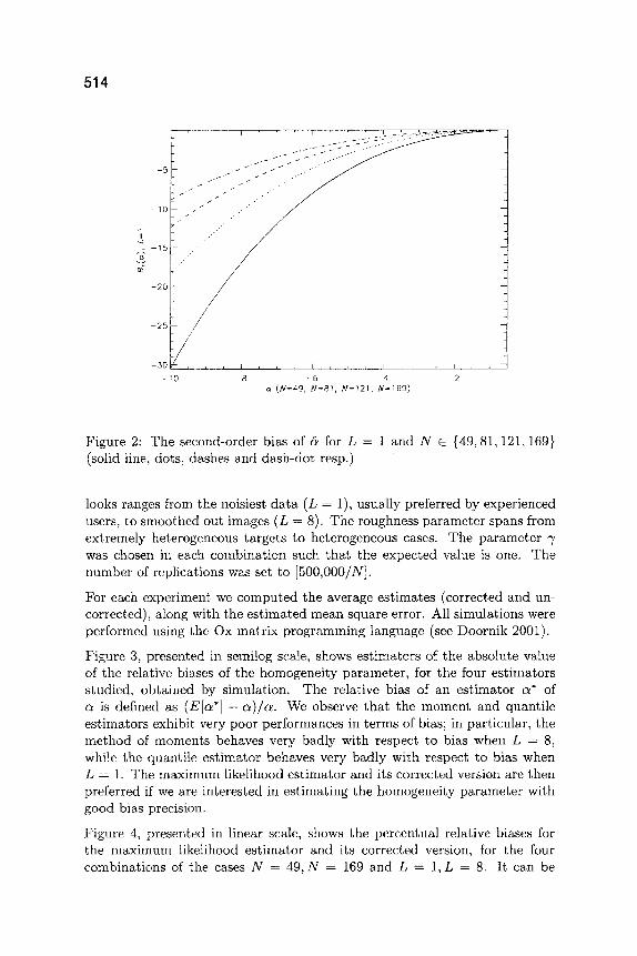
Figure 2: The second-order bias of & for L = 1 and N E {49, 81,121,169} (solid line, dots, dashes and dash-dot resp.)

looks ranges from the noisiest da t a (L = 1), usual ly preferred by experienced users, to smoothed out images (L = 8). The roughness pa ramete r spans from extremely heterogeneous targets to heterogeneous cases. The pa ramete r 7 was chosen in each combinat ion such tha t the expected value is one. The number of replications was set to [500,000/N].

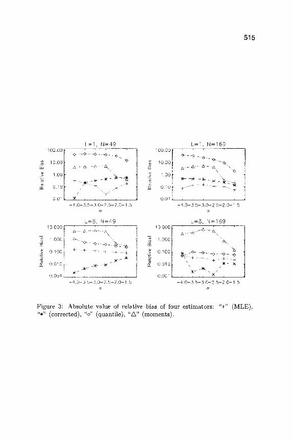
For each experiment we computed the average es t imates (corrected and un- corrected), along with the es t imated mean square error. All s imulat ions were performed using the Ox mat r ix programming language (see Doornik 2001).

Figure 3, presented in semilog scale, shows es t imators of the absolute vahm of the relative biases of the homogeneity parameter , for the four es t imators studied, obta ined by simulation. The relat ive bias of an es t imator ct* of ct is defined as (E[a*] - ~)/a. We observe tha t the moment and quanti le es t imators exhibit very poor performances in terms of bias; in par t icular , the method of moments behaves very badly with respect to bias when L = 8, while the quant i le es t imator behaves very bad ly with respect to bias when L = 1. The maximum likelihood es t imator and its corrected version are then preferred if we are interested in es t imat ing the homogenei ty pa ramete r with good bias precision.

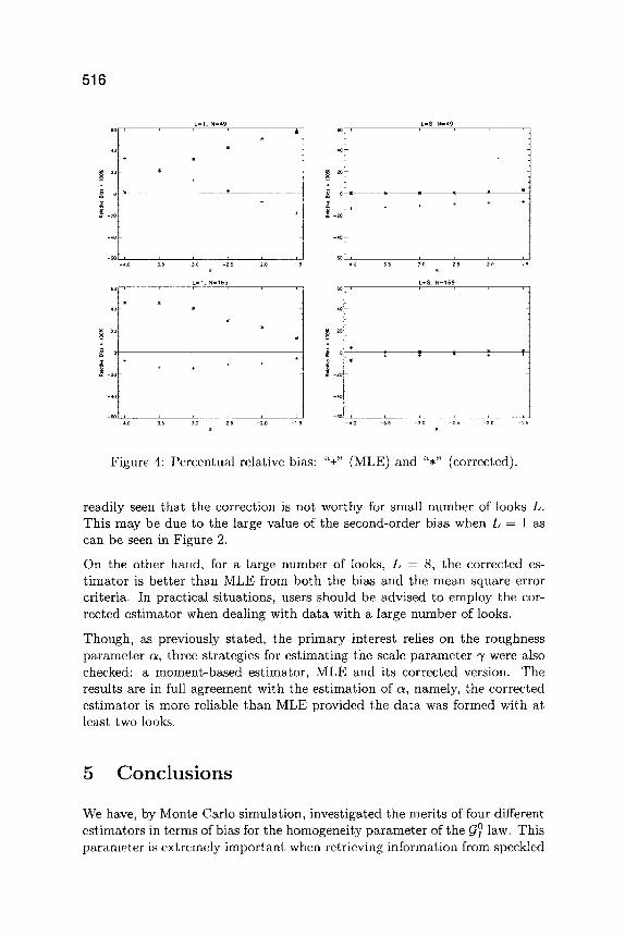
Figure 4, presented in linear scale, shows the percentual relative biases for the max imum likelihood es t imator and its corrected version, for the four combinat ions of the cases N = 49, N = 169 and L = 1, L = 8. I t can be

515

1 0 0 . 0 0

% 1 0 . 0 0

1 . 0 0

o

~ 0 . 1 0

0.01

1 0 0 0 0

% 1 0 0 0

~ O.lO0 o

0 . 0 1 0

0 . 0 0 1

L= 1, N=49

@ - + - - ~ - - - < > - . ~ . r

, - ~

5. - - - A - - - A - - "

/ "" %. . .-t- / . ,4"

u -- 4 .0 - -D .5 - - } , O i 2 ,5 - - 2 .0 - - 1 .5

,3:

L=8, N=49 k ~ - - s - - - e 2 - - - ,,,,

\

0 , - .

+ - 4,. .-+-.. , + . . . + + . .§

- 4 . 0 - 3 5 - , 3 . 0 - 2 . 5 - 2 , 0 - 1 . 5

1 0 0 . 0 0

1 0 . 0 0 !

1.00

0 . 1 0

0 .01

10.000

1 . 0 0 0

0 . 1 0 0

0 . 0 1 0

0.001

L = I , N=169

A . f ~ - - - A - - - A \ ,

~ - --~-- --~4- _ ~ ~ , . . . + . . . + " " / - " ' - + - - ~ C ' 2 ~

-~ . . . . . . +

4 . 0 - , 3 . 5 - 3 . 0 - 2 . 5 - 2 . 0 - 1 . 5

O(

L=8, N=169

N

~7 + " " + " - + " + '" + \ )I( - -.~ \

x /

- 4 . 0 - 3 . 5 - 3 . 0 - 2 . 5 - 2 . 0 - 1 . 5

Figure 3: Absolute value of relative bias of four estimators: "+" (MLE), "*" (corrected), "o" (quantile), "a" (moments).

5 1 6

eo ,

,m +

~~

-40

-SO , -4 .O

so

40

~ 2o

- 4 . O

L=I, N=49 L=8, N=49

0 iI -20 I -40

eO i - 4 . o

+ + +

L=I. N=169 L=8, N~169 IE 4 0

! i t , , , , ,

- 2 e

3 S - 3 , 0 - Z 5 - 2 , 0 -~ ,5 - 4 . 0 - 3 5 - 3 0 - 2 S - ~ 0 - ~ 5

Figure 4: Percentual relative bias: "+" (MLE) and "*" (corrected).

readi ly seen tha t the correction is not worthy for small number of looks L. This may be due to the large value of the second-order bias when L = 1 as can be seen in Figure 2.

On the other hand, for a large number of looks, L = 8, the corrected es- t ima to r is be t te r than MLE from both the bias and the mean square error criteria. In pract ical s i tuat ions, users should be advised to employ the cor- rected es t imator when dealing with da t a with a large number of looks.

Though, as previously s tated, the pr imary interest relies on the roughness pa ramete r a , three strategies for es t imat ing the scale pa ramete r ~/were also checked: a moment-based es t imator , MLE and its corrected version. The results are in full agreement with the es t imat ion of a , namely, the corrected es t imator is more reliable than MLE provided the da t a was formed with at least two looks.

5 C o n c l u s i o n s

We have, by Monte Carlo simulat ion, invest igated the meri ts of four different es t imators in terms of bias for the homogenei ty pa ramete r of the g0 law. This pa ramete r is ext remely impor tan t when retr ieving information from speckled

517

imagery.

Based on our simulation experience, we can conclude that all four estimators may present different estimation problems. The method of moments should work only if we assume the respective moments to be finite and may produce large mean square errors. The quantile estimator introduces a complicated nonlinear system of equations. The maximum likelihood may be very flat, depending on the situation. Finally, the corrected estimator may produce values outside the feasible range.

Based on the numerical results of our simulations, we observe that the maxi- mum likelihood estimator and its corrected version are the preferred inference procedures with respect to bias. We have also verified that there is a wide range of practical situations for which the corrected estimator effectively re- duces both bias and mean square error of the original Maximum Likelihood estimator. The evaluation of the corrected estimator is affordable from the computational point of view, not depending on cumbersome functions and not introducing numerical instabilities.

The corrected estimator is recommended when the sample size is at least 100 and when the imagery has been processed to have at least two looks. In both cases the information ill tile sample about c~ is sufficiently large to yield reliable corrected estimators.

Inference strategies for the recently proposed multivariate version of the dis- tribution (see Freitas, Frery & Correia in press) here considered in under assessment.

A c k n o w l e d g e m e n t s

We gratefully acknowledge partial financial support from CNPq, Brazil.

R e f e r e n c e s

Bustos, O. H., Lucini, M. M. & Frery, A. C. (2002), 'M-estimators of rough- ness and scale for GA0-modelled SAR imagery', EURASIP Journal on Applied Signal Processing 2002(1), 105-114.

Cordeiro, G. & Vasconcellos, K. (1999), 'Second-order biases of the maximum likelihood estimates in von-Mises regression models', Australian and New Zealand Journal of Statistics 41,901-910.

Cox, D. R. & Snell, E. J. (1968), 'A general definition of residuals (with discussion)', Journal of the Royal Statistical Society B 30, 248-275.

518

Cribari-Neto, F. & Vasconcellos~ K. L. P. (2002), 'Nearly unbiased maximum likelihood estimation for the beta distribution', Journal of Statistical Computing and Simulation 72(2), 107 118.

Cribari-Neto, F., Frery, A. C. ~: Silva, M. F. (2002), 'Improved estimation of clutter properties in speckled imagery', Computational Statistics and Data Analysis 40(4), 801-824.

Doornik, J. A. (2001), Ox: an object-oriented matrix programming language, 4 edn, Timberlake Consultants ~z Oxford, London.

Firth, D. (1993), 'Bias reduction of maximum likelihood estimates', Biometrika 80, 27-38.

Freitas, C. C., Frery, A. C. & Correia, A. H. (in press), 'The polarimetric G distribution for SAR data analysis', Environmetrics.

Frery, A. C., Cribari-Neto, F. & Souza, M. O. (in press), 'Analysis of minute features in speckled imagery with maximum likelihood estima- tion', EURASIP Journal on Applied Signal Processing.

Frery, A. C., Miiller, H.-J., Yanasse, C. C. F. ~ Sant'Anna, S. J. S. (1997a), 'A model for extremely heterogeneous clutter', IEEE Transactions on Ceoscience and Remote Sensing 35(3), 648-659.

Frery, A. C., Sant'Anna, S. J. S., Mascarenhas, N. D. A. & Bustos, O. H. (1997b), 'Robust inference techniques for speckle noise reduction in l- look amplitude SAR images', Applied Signal Processing 4, 61-76.

Goodman, J. W. (1976), 'Some fundamental properties of speckle', Journal of the Optical Society of America 66, 1145-1150.

Goodman, N. R. (1963), 'Statistical analysis based on a certain complex Gaussian distribution (an introduction)', Annals of Mathematical Statis- tics 34, 152-177.

Gradshteyn, I. S. ~ Ryzhik, I. M. (1980), Table of Integrals, Series and P~vducts, Academic Press, New York.

Jr B. (1982), Statistical Properties of the Generalized Inverse Gaus- sian Distribution, Vol. 9 of Lecture Notes in Statistics, Springer-Verlag, New York.

Mejail, M. E., Frery, A. C., Jacobo-Berlles, J. &: Bustos, O. H. (2001), 'Ap- proximation of distributions for SAR images: proposal, evaluation and practical consequences', Latin American Applied Research 31, 83 92.

Mejail, M. E., Jacobo-Berlles, J., Frery, A. C. & Bustos, O. H. (2000), 'Para- metric roughness estimation in amplitude SAlt images under the multi- plicative model', Revista de Teledeteccidn 13, 37-49.

519

Mejail, M. E., Jacobo-Berlles, J., Frery, A. C. & Bustos, O. H. (2003), 'Clas- sification of SAR images using a general and tractable multiplicative model', International Journal of Remote Sensing 24(18), 3565-3582.

Oliver, C. & Quegan, S. (1998), Understanding Synthetic Aperture Radar Images, Artech House, Boston.

Pike, M., Hill, A. & Smith, P. (1980), 'Bias and etticiency in logistic analysis of stratified case-control studies', International Journal of Epidemiology 9, 89-95.

Seshadri, V. (1993), The Inverse Gaussian Distribution: A Case Study in Exponential Families, Claredon Press, Oxford.

Young, D. & Bakir, S. (1987), 'Bias correction for a generalized log-gamma regression model', Technometr'ics 29, 183-191.