eScholarship provides open access, scholarly publishingservices to the University of California and delivers a dynamicresearch platform to scholars worldwide.

California Partners for Advanced Transitand Highways (PATH)

UC Berkeley

Title:An Analytical Dynamic Traffic Assignment Model with Probabilistic Travel Times and Travelers'Perceptions

Author:Liu, Henry X.Ban, XuegangRan, BinMirchandani, Pitu

Publication Date:07-01-2002

Series:Working Papers

Publication Info:Working Papers, California Partners for Advanced Transit and Highways (PATH), Institute ofTransportation Studies, UC Berkeley

Permalink:http://escholarship.org/uc/item/49h9x0wh

Abstract:Dynamic traffic assignment (DTA) has been a topic of substantial research during the past decade.While DTA is gradually maturing, many aspects of DTA still need improvements, especiallyregarding its formulation and solution capabilities under the transportation environment impactedby the Advanced Transportation Management and Information Systems (ATMIS). It is necessaryto develop a set of DTA models to acknowledge the fact that the traffic network itself is probabilisticand uncertain, and different classes of travelers respond differently under uncertain environment,given different levels of traffic information. This paper aims to advance the state-of-the-art inDTA modeling in the sense that the proposed model captures the travelers(tm) decision makingamong discrete choices in a probabilistic and uncertain environment, in which both probabilistictravel times and random perception errors that are specific to individual travelers, are considered.Travelers(tm) route choices are assumed to be made with the objective of minimizing perceiveddisutilities at each time. These perceived disutilities depend on the distribution of the variable routetravel times, the distribution of individual perception errors and the individual traveler(tm)s risktaking nature at each time instant. We formulate the integrated DTA model through a variationalinequality (VI) approach. Subsequently, we discuss the solution algorithm for the formulation.Experimental results are also given to verify the correctness of solutions obtained.

CALIFORNIA PATH PROGRAMINSTITUTE OF TRANSPORTATION STUDIESUNIVERSITY OF CALIFORNIA, BERKELEY

This work was performed as part of the California PATH Program ofthe University of California, in cooperation with the State of CaliforniaBusiness, Transportation, and Housing Agency, Department of Trans-portation; and the United States Department Transportation, FederalHighway Administration.

The contents of this report reflect the views of the authors who areresponsible for the facts and the accuracy of the data presented herein.The contents do not necessarily reflect the official views or policies ofthe State of California. This report does not constitute a standard,specification, or regulation.

ISSN 1055-1417

July 2002

An Analytical Dynamic Traffic AssignmentModel with Probabilistic Travel Times andTravelers’ Perceptions

California PATH Working PaperUCB-ITS-PWP-2002-6

CALIFORNIA PARTNERS FOR ADVANCED TRANSIT AND HIGHWAYS

Henry X. Liu, Xuegang Ban,Bin Ran, Pitu Mirchandani

Report for TO 4100

An Analytical Dynamic Traffic Assignment Model with ProbabilisticTravel Times and Perceptions

Henry X. Liu a, Xuegang Ban b, Bin Ran b, Pitu Mirchandani c

a California PATH Program, University of California, Berkeleyb Department of Civil and Environmental Engineering, University of Wisconsin at Madison

c Department of System Engineering, University of Arizona

ABSTRACT

Dynamic traffic assignment (DTA) has been a topic of substantial research during thepast decade. While DTA is gradually maturing, many aspects of DTA still needimprovements, especially regarding its formulation and solution capabilities under thetransportation environment impacted by the Advanced Transportation Management andInformation Systems (ATMIS). It is necessary to develop a set of DTA models toacknowledge the fact that the traffic network itself is probabilistic and uncertain, anddifferent classes of travelers respond differently under uncertain environment, givendifferent levels of traffic information. This paper aims to advance the state-of-the-art inDTA modeling in the sense that the proposed model captures the travelers� decisionmaking among discrete choices in a probabilistic and uncertain environment, in whichboth probabilistic travel times and random perception errors that are specific to individualtravelers, are considered. Travelers� route choices are assumed to be made with theobjective of minimizing perceived disutilities at each time. These perceived disutilitiesdepend on the distribution of the variable route travel times, the distribution of individualperception errors and the individual traveler�s risk taking nature at each time instant. Weformulate the integrated DTA model through a variational inequality (VI) approach.Subsequently, we discuss the solution algorithm for the formulation. Experimental resultsare also given to verify the correctness of solutions obtained.

1. INTRODUCTION

Over the past several decades, various traffic assignment models have been developedbased on whether network attributes are dynamic or time-dependent, whether networkstochasticity is considered in the travelers� decision making, and whether travelers� routetravel time perception errors are assumed. Following Chen�s classification (1) andconsidering both static and dynamic cases in general, traffic assignment models can becategorized as in Table 1.

Table 1. Classification of Traffic Assignment Models

Accurate Perception Inaccurate PerceptionDeterministic Network DN-UE DN-SUEStaticStochastic Network SN-UE SN-SUEDeterministic Network DN-DUO DN-SDUODynamicStochastic Network SN-DUO SN-SDUO

2

Where: DN = Deterministic Network SN = Stochastic Network UE = User Equilibrium SUE = Stochastic User Equilibrium DUO = Dynamic User Optimal SDUO = Stochastic Dynamic User Optimal

Among those models in Table 1, the static user equilibrium (UE) models are usually usedfor the long-term planning purpose (2). Most of them are formulated to be consistent withthe Wardrop�s first principle. This principle requires that, for used routes between a givenorigin-destination (OD) pair, the route cost equals the minimum route cost, and no usedroute has a lower cost. The basic assumption in the UE models is that over some periodof time, each traveler learns and adapts to the transportation network conditions and theservices available to him/her so that an equilibrium can be reached. In the DN-UE model,no network uncertainty is considered, i.e. link travel times are deterministic and eachtraveler is assumed to have perfect knowledge of the network travel times on all possibleroutes between his/her OD pair. To overcome the deficiencies of the deterministic model,DN-SUE model relaxes the assumption of travelers� perfect knowledge of network traveltimes, allowing travelers to select routes based on their perceived travel times. However,given that travel time uncertainty is one of the important factors in route choice as shownin a recent empirical study by Abdel-Aty et al. (7), a realistic route choice model shouldcapture the tradeoffs between expected travel time and travel time uncertainty in decisionmaking. The SN-SUE model falls in this category.

On the other hand, with continuous information and advice from AdvancedTransportation Management and Information System (ATMIS), static UE may not existbut rather the travelers choose routes and modes based on the current perceived conditionof the traffic on the network (3). Therefore, the dynamic generalization of the static UEconcept is called the dynamic user optimal (DUO). One DUO traffic assignment problemis to determine vehicle flows at each instant of time on each link resulting from driversusing minimal-time routes. Thus, we are no longer considering day-to-day trafficequilibrium. Instead, we are trying to influence or control traffic and travel patterns oftravelers optimally by providing accurate traffic information and effective traffic controlmeasures. In a simple DTA model, all users of the network have perfect information onthe travel times on the network and choose routes which minimize either their traveltimes or some generalized cost. Such a DTA model is typically deterministic. But in reallife, since one might expect that network travel times for a given set of flows arestochastic in nature and also the travelers may not have perfect information about thenetwork, the deterministic assumptions are questionable.

A large body of work is available on stochastic user equilibrium models. Dial was amongthe first to present the algorithm to assign link flows based on a logit model and later thisstochastic user equilibrium model on deterministic networks (DN-SUE) was formulatedas an optimization problem (4). In the generalized SN-SUE model (5), proposed byMirchandani and Soroush, the travel time on each route is random and each traveler

3

perceives inaccurately. Thus, the perceived distribution of travel times for each traveler isa function of the actual distribution of the network travel times as well as the distributionof the traveler�s own perception error. Furthermore, because it is assumed that travelersare aware of the variable nature of travel times on the network, the decision makingprocess involved in choosing a route is assumed to represent risk taking behavior underuncertainty. Since route choice decisions usually involve tradeoffs between expectedtravel time and travel time uncertainty, Tatineni indicated that it may be appropriate tomodel travelers as either risk averse, risk prone or risk neutral, and the risk in this case isthe variability associated with route travel times (6). Chen and Recker examined theeffect of considering risk taking behavior in static route choice models and its impact onthe estimation of travel time reliability of a road network subject to demand and supplyvariations (1).

In order to realize the real-time traffic network monitoring and management function inATMIS, a SN-SDUO model that captures travelers� route choice behavior in a dynamicand stochastic transportation network needs to be developed. In this model, it is essentialto understand how drivers make route choices, especially in the light of the considerableinformation that the driver may receive within ITS environment, such as variablemessage signs (VMS), highway advisory radio (HAR), and in-vehicle navigationsystems, etc. Along with the driver�s prior knowledge of the traffic network, such amodel, as shown in Figure 1, should replicate, to the extent possible, the driver�sperception of available routes and his or her decision-making in selecting the routes.Based on different assumptions on the distributions of actual route travel time andperceived route travel time error, various DTA models can be obtained. Most of currentstochastic DTA models consider either a stochastic route travel time without travelerperception error such as Boyce�s model (8) or deterministic network with travelerperception error such as Ran�s model (9), but not both. To our knowledge, no SN-SDUOmodel has been proposed in the literature.

Cognitive ModelDTA ModelSN-SDUO

Traffic Networkand Conrol

TravelAdvisories

andTraffic

Information

DynamicStochastic

ActualTravel Times

Perceptions

PredictedTraffic

Figure 1. DTA Model with Probabilistic Travel Time and Perceptions

The objective of this paper is to propose a formulation and solution algorithm for the SN-SDUO model, which is a stochastic dynamic user optimal model based on stochastic

4

dynamic network. This paper extends Mirchandani and Soroush�s generalized trafficequilibrium (5) into a dynamic environment. The assumption is that route travel times arevariable and perceived as such by travelers at each time instant. Each traveler uses adisutility function of travel time to evaluate each route and route choices are assumed tobe made with the objective of minimizing perceived disutility at each time and no travelercan reduce his/her perceived expected disutility by changing to another route. Theseperceived disutilities depend on the distribution of the variable route travel times, thedistribution of individual perception errors, and the individual traveler�s risk takingnature at each time. By considering the traveler�s risk-taking behavior in dynamic andprobabilistic environment, the proposed model can capture the traveler�s route choicecharacteristics such that a trade-off decision between a route with longer but reliabletravel time versus another route with shorter but unreliable travel time.

This paper is organized as follows. The dynamic user-optimal route choice conditions areformulated and then a variational inequality (VI) is derived in Section 2. Traveler�sperception under dynamic and stochastic network, the stratification of traveler�s risk-taking behavior, and the route choice characteristics of these traveler classes will also bediscussed in this section. In Section 3, we discuss an algorithm that can solve the VIformulation via a combination of relaxation technique, stochastic network loading, andMethod of Successive Averages (MSA). Section 4 contains some computational resultsof applying the proposed approach to several simple scenarios, with the objective ofverifying solution qualities. Finally, concluding remarks are discussed in Section 5.

2. THE VARIATIONAL INEQUALITY FORMULATION

2.1 Notation

In the following, superscript �rs� denotes origin-destination pair rs, subscript �a� (or�b�) denotes link a (or b), subscript �p� (or � ~p �) denotes path p (or subpath ~p betweennode j and destination s), and subscript �m� denotes traveler class m. All the variablesused in the formulation are defined as follows:xa(t) = number of vehicles on link a at time t (main problem variable)ua(t) = inflow rate into link a at time t (main problem variable)va(t) = exit flow rate from link a at time t (main problem variable)ya(k) = number of vehicles on link a at the beginning of time interval k (subproblem

variable))(� ky i

a = number of vehicles on link a at the beginning of time interval k at iteration i

(stochastic loading loop)pa(k) = inflow into link a during interval k (subproblem variable)

)(� kpia

= inflow into link a during interval k at iteration i (stochastic loading loop)

qa(k) = exit flow from link a during interval k (subproblem variable)

)(� kqia

= exit flow from link a during interval k at iteration i (stochastic loading loop)

f tmrs ( ) = class m departure flow rate from origin r to destination s at time t (given)

f tpmrs ( ) = class m departure flow on path p from origin r to destination s at time t

5

ers(t) = arrival flow rate from origin r toward destination s at time tErs(t) = cumulative number of vehicles arriving at destination s from origin r by time

t (main problem variable)E k

rs( ) = cumulative number of vehicles arriving at destination s from origin r during

interval k (subproblem variable)A(j) = set of links whose tail node is j (after j)B(j) = set of links whose head node is j (before j)P tp

rs( ) = proportion of flows between (r,s) that follow route p at time t

ta(t) = actual travel time over link a for flows entering link a at time t

t a t( ) = estimated mean actual travel time over link a for flows entering link a attime t

Ta(t) = perceived travel time over link a for flows entering link a at time t)(tph = actual travel time for route p between (r, s) for flows departing origin r at

time t)(tpW = perceived travel time for route p between (r, s) for flows departing origin r

at time t)(tpx = perceived travel time error for route p between (r, s) for flows departing

origin r at time tRrs(t) = the set of path between (r, s) at time tp rs t( ) = minimal disutility between (r, s) for flows departing origin r at time tDU tp

rs ( ) = perceived disutility for route p between (r,s) for flows departing origin r at

time t

2.2 Traveler�s Perceptions Under Dynamic and Stochastic Network

Consider a traffic network represented by a directed graph consisting of a finite set ofnodes and links. We assume that the travel times for traversing the links in the networkare random variable and the probability density functions (PDF) of link travel times aredependent on the time when a link is entered. Therefore, the link travel time ta(t) can be

modeled as a stochastic process. The stochasticity of the link travel time for a given set offlows on the traffic network could be resulted from different sources such as differentweather conditions, different mix of vehicle types, and different delays experienced bydifferent vehicles at intersections, etc. Incidents, such as vehicle breakdowns and signalfailure, also contribute to the random effects of the traffic network. A network where thelink travel time is modeled as a stochastic process is referred to as a dynamic andstochastic network (10).

The accuracy of a traveler perception of the network depends on the traveler�s perviousexperience during similar network flow conditions and information available to thetraveler from various sources such as travel time updates via radio, television, internet oradvanced traveler information systems. In reality, travelers may have either or bothimperfect information and different perceptions towards travel time rather than perfectinformation and homogeneous perceptions.

6

Let there be M different groups of travelers, where the travelers of each group have thesame disutility function and same perception error distribution. In this paper, we assumethat each traveler i from group m perceives the travel time on link a of route p at time t asa distribution comprising of the distribution of actual link travel time )(tat and a

perception error )(timax , whose distribution parameters are specific to traveler i.

misrtRppatttT rsimaa

ima ,,, ),( ,),()()( "��+= xt (1)

Assume route p consists of nodes (r, 1, 2, �,s). Then, a recursive formula for theperceived route travel time )(trs

pW is:

)()()()( 1111 tTttt rrrrp =+=W xt (2)

�; ,...,2 j ;,,))(()()( )1()1( sjrpttTtt jr

pajr

prjp ="W++W=W -- (3)

where link a = (j-1, j). Theoretically, we will have:

psrttttttTts

j

jrpa

jrpa

s

j

jrpa

rsp ,, )))(())((())(()(

1

)1()1(

1

)1( "W++W+=W+=W ÂÂ=

--

=

- xt (4)

Equation (4) shows that the perceived route travel time is a random variable where theparameters of its associate probability density function (PDF) are dependent on thedistribution of traveler�s perception error as well as on the distribution of actual routetravel time. Depending on the level of available travel time information (this includestraveler�s previous knowledge) at different time period, the distribution of travelerperception error may vary dynamically. This in itself requires extensive empiricalinvestigation; and the distribution may not be able to be represented by an algebraicfunction even after that. To make the model somewhat tractable, the followingassumptions are made in this paper.

Assumption 1: At time instant t, the perceived error )(timx of an individual i from group

m for a segment of road with unit travel time has normal distribution ))(),(( ttN imim qm .

The parameters )(timm and )(timq are dependent on the level of travel time informationavailable to the traveler at time t. Therefore, we also assume:

)),(()( ttInfoft imimim mm = (5)

)),(()( ttInfogt imimim qq = . (6)

Here, )(tInfoimrepresents the available travel time information to the traveler i from group

m at time t, f and g are functional relationships. The parameters imm and imq for a random

individual i from group m have normal distribution ),0( mN t and gamma distribution

),( mmG ba over the population, respectively. Here, mt , ma and mb are some constantvalues which are specific to group m.

7

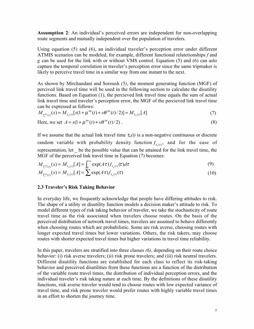
Assumption 2: An individual�s perceived errors are independent for non-overlappingroute segments and mutually independent over the population of travelers.

Using equation (5) and (6), an individual traveler�s perception error under differentATMIS scenarios can be modeled, for example, different functional relatetionships f andg can be used for the link with or without VMS control. Equation (5) and (6) can aslocapture the temporal correlation in traveler�s perception error since the same tripmaker islikely to perceive travel time in a similar way from one instant to the next.

As shown by Mirchandani and Soroush (5), the moment generating function (MGF) ofpercived link travel time will be used in the following section to calculate the disutilityfunctions. Based on Equation (1), the percieved link travel time equals the sum of actuallink travel time and traveler�s perception error, the MGF of the percieved link travel timecan be expressed as follows:

][)]2/)()(1([)( )()()(AMtstsMsM t

imimttT aa

ima

tt qm =++= (7)

Here, we set )2/)()(1( tstsA imim qm ++= . (8)

If we assume that the actual link travel time ta(t) is a non-negative continuous or discrete

random variable with probability density function )(taft , and for the ease of

representation, let _ be the possible value that can be attained for the link travel time, theMGF of the perceived link travel time in Equation (7) becomes:

ttt tt dfAAMsM tttT aaim

a)()exp(][)(

0 )()()( Ú+�

== (9)

)()exp(][)( )()()(tt tt tttT aa

ima

fAAMsM Â== (10)

2.3 Traveler�s Risk Taking Behavior

In everyday life, we frequently acknowledge that people have differing attitudes to risk.The shape of a utility or disutility function models a decision maker�s attitude to risk. Tomodel different types of risk taking behavior of traveler, we take the stochasticity of routetravel time as the risk associated when travelers choose routes. On the basis of theperceived distribution of network travel times, travelers are assumed to behave differentlywhen choosing routes which are probabilistic. Some are risk averse, choosing routes withlonger expected travel times but lower variations. Others, the risk takers, may chooseroutes with shorter expected travel times but higher variations in travel time reliability.

In this paper, travelers are stratified into three classes (6), depending on their route choicebehavior: (i) risk averse travelers; (ii) risk prone travelers; and (iii) risk neutral travelers.Different disutility functions are established for each class to reflect its risk-takingbehavior and perceived disutilities from these functions are a function of the distributionof the variable route travel times, the distribution of individual perception errors, and theindividual traveler�s risk taking nature at each time. By the definitions of these disutilityfunctions, risk averse traveler would tend to choose routes with low expected variance oftravel time, and risk prone traveler would prefer routes with highly variable travel timesin an effort to shorten the journey time.

8

Following the study by Tatineni et al. (6), we also use the exponential disutility function,which is one of the most widely used disutility functions reported in the decision-makingliterature to model the different risk taking behaviors. The shapes of these different risktaking behaviors are provided in Figure 2.

Figure 2. Disutility Functions for Different Risk-Taking Route Choice Models

To calculate the perceived expected disutility functions, the perceived route travel time isneeded. A naive approach is to enumerate all paths, derive the PDF of the perceivedtravel time of these paths, and then compute the corresponding perceived expecteddisutilities. However, this could take considerable computational effort for even a smallnetwork. One important advantage of using the exponential function is that the disutilityassociated with a route can be estimated by summing the link disutilities on that route.This allows the classical Dijkstra-type shortest path algorithm to be used in finding theminimum expected disutility route. As discussed by Mirchandani and Soroush (5), theMGF of perceived route travel time in Equation (7) and (8) could be used to calculate theexpected disutility functions, without the requirement of path enumeration. We presentthe results in the following. In all cases, we assume that a route with 0 minutes traveltime has a disutility of 0 and a route with 5 minutes travel time has a disutility of 1.Assume route p from origin r to destination s consists of j intermediate nodes, j= (1, 2,�,s), and link a = (j-1, j) is on the route p.

For the risk averse case, the disutility function of a risk averse person takes the form of:21 ))(exp()( atatDU rs

prsp -W= a (11)

The perceived expected disutility function is:

2))((1 )())(( )1( aMatDUEpa

ttT

rsp jr

pa-= �

�W+ - a (12)

With the boundary conditions and the risk averse assumption, the disutility function andthe perceived expected disutility function finally have the forms of:

)1))(289.0(exp(309.0)( -W= ttDU rsp

rsp (13)

0

0.2

0.4

0.6

0.8

1

1.2

0 0.5 1 1.5 2 2.5 3 3.5 4 4.5 5

Travel Time (min)

Dis

utili

ty

RA

RP

RN

9

)1)289.0((309.0))(())(( )1( -= �

�W+ -

pattT

rsp jr

paMtDUE (14)

For the risk prone case, the disutility function of a risk prone person takes the form of:))(exp()( 12 tbbtDU rs

prsp W--= b (15)

The perceived expected disutility function is:)())((

))((12 )1( b--= ��

W+ -

pattT

rsp jr

paMbbtDUE (16)

With the boundary conditions and the risk averse assumption, the disutility function andthe perceived expected disutility function finally have the forms of:

)))(289.0exp(1(309.1)( ttDU rsp

rsp W--= (17)

))289.0(1(309.1))(())(( )1( --= �

�W+ -

pattT

rsp jr

paMtDUE (18)

For the risk neutral case, the disutility function is a linear function with the expectedperceived travel time. For the ease of modeling, we use exponential form to approximatelinear disutility function. Therefore, the disutility function of a risk neutral person takesthe form of:

))(exp()( 12 tcctDU rsp

rsp W--ª g (19)

The perceived expected disutility function is:)())(( )(12 g--ª �

�patT

rsp a

McctDUE (20)

With the boundary conditions and the risk neutral assumption, the disutility function andthe perceived expected disutility function finally have the forms of:

)))(01.0exp(1(5.20)( ttDU rsp

rsp W--ª (21)

))01.0(1(5.20))(( )( --ª ��pa

tTrsp a

MtDUE (22)

For comparison purpose, note that risk neutral travelers make route choice decisionsbased on the mean perceived route travel times solely, regardless the variance ofperceived route travel times. Essentially, risk neutral travelers consider the route traveltime as deterministic in the sense that all routes have the mean travel times. So if weassume that all travelers are risk neutral, our SN-SDUO model becomes DN-SDUO.

2.4 The Dynamic Network Constraint Set

The constraint set for our DTA problem is summarized for each class of travelers.

Route Flow Assignment Constraints:f t f t P t where f t is given r s p mpm

rsmrs

prs

mrs( ) ( ) ( ) ( ) , , , ;= " (23)

f t u t r s p m a A r a ppmrs

apmrs( ) ( ) , , , ; ( ); ;= " � � (24)

Other Constraints for all traveler classes:

10

Relationship between state and control variables:dx

dtu t v t m a p r sapm

rs

apmrs

apmrs= - "( ) ( ) , , , , (25)

dE t

dte t p m r s rpm

rs

pmrs( )

( ) , , ;= " π (26)

Flow conservation constraints:v t u t j p m r s j r sapm

rsapmrs

a A ja B j

( ) ( ) , , , , ; ,( )( )

= " π��

ÂÂ (27)

v t e t m r s s rapmrs

pmrs

pa B s

( ) ( ) , , ;( )

= " πÂÂ�

(28)

Flow propagation constraints:x t x t t x t E t t E t a B j j r p r sap

rsbprs

ab p

bprs

prs

a prs( ) { [ ( )] ( )} { [ ( )] ( )} ( ); ; ; ;

~= + - + + - " � π

�

 t t (29)

Definitional constraints:u t u t v t v t x t x t aapm

rsa

rspmapmrs

a apmrs

arspmrspm

( ) ( ), ( ) ( ), ( ) ( ),= = = "Â ÂÂ (30)

Nonnegativity conditions:x t u t v t m a p r sapm

rsapmrs

apmrs( ) , ( ) , ( ) , , , , ,≥ ≥ ≥ "0 0 0 (31)

f t e t E t p m r spmrs

pmrs

pmrs( ) , ( ) , ( ) , , , ,≥ ≥ ≥ "0 0 0 (32)

Boundary conditions:E p m r spm

rs ( ) , , , ,0 0= " (33)

x a p m r sapmrs( ) , , , , ,0 0= " . (34)

For each class of travelers, the constraints expressed in (23) - (34), including flowpropagation and conservation constraints, are applicable. These constraints are used togenerate path and link flows when route departure flows are determined. The pathdeparture flow f tp

rs ( ) is determined by the stochastic loading function. The link flow

propagation constraints (29) are implemented for each link a, each route p, each O-D pairrs, and each time t, regardless of traveler classes. Therefore, the FIFO requirement can beensured.

2.4 Link Travel Time and Delay Functions

Since a stochastic network is considered in this paper, variation of the link travel timeshould be required. Thus, in this paper, the actual link travel time ta(t) has two

components: one is deterministic flow-dependent cruise time ca(t) and the other one is thestochastic delay da(t). The stochastic delay may be caused by the traffic signal at theintersection for an arterial link or by the congestion for a freeway link.

There are various cruise time functions for different link types, such as freeway andarterial. To simplify the computation, it is assumed that the cruise time depends on thenumber of vehicles and the inflow rate. Equation (35) shows the link cruise time functionchosen for the numerical results of this study:

11

ax

x

C

uTtxtuctc

a

a

a

afaaaaa "++== ])(1[)](),([)(

max,,

ab (35)

where a and b are coefficients, Ta f, is the free flow travel time on link a , Ca is its

capacity, and xa,max is its maximum holding capacity.

In this paper, to simplify our algorithm, the stochastic delay is modeled as a non-negativenormal distribution, which relates directly to the cruise time of this link, as shown inEquation (36).

),( 2aaaaa ccNd sm= (36)

where am is the mean parameter and 2as is the variance parameter.

2.5 The VI Formulation

Assume travelers are disutility minimizers. The probability that route p is chosen by anindividual can be stated as follows:

))),(())(((Prob)( tDUEtDUEtP rsq

rsp

rsp £= " route q between r and s, "r, s, p. (37)

where Prob is the choice function representing the proportion of individuals who chooseroute p. The DUO route choice conditions are then defined as follows:

f t f t P t r s pprs rs rs( ) ( ) ( ) , ,- = "0 (38)

Note that the mean actual route travel time h prs t( ) is increasing with path departure flow

f tprs ( ) , i.e.,

∂h∂

prs

prs

t

f tr s p

( )

( ), ,> "0 (39)

For each path p and each O-D pair rs, define an auxiliary cost term as follows:

F t f t f t P tt

f tr s pp

rsprs rs

prs p

rs

prs

( ) [ ( ) ( ) ( )]( )

( ), ,= - = "

∂h∂

0 (40)

It is obvious that the above equality states the DUO route choice conditions, since∂h ∂p

rsprst f t( ) / ( ) > 0 . As shown in (11), the above system of equations is equivalent to the

following variational inequality for each time instant t � +�[ , )0 :

F t f t f tprs

prs

prsprs( ){ ( ) ( )}*- ≥ 0 (41)

where superscript * denotes that path departure flow f has an optimal value. SinceF tp

rs ( ) = 0 , the above inequality is also equivalent to the integral form:

F t f t f t dtprs

prs

T

prs

prs( ){ ( ) ( )}*ÂÂÚ - ≥

00 (42)

3. THE SOLUTION ALGORITHM

To solve the VI problem, we need to convert our continuous time VI problem into adiscrete time VI problem. The time period [0,T] is subdivided into K small time intervals.Each time interval is regarded as one unit of time. Then, ua(k) represents the inflow intolink a during interval k, va(k) represents the exit flow from link a during interval k, x ka ( )

12

represents the number of vehicles at the beginning of interval k, and fp(k) represents thedeparture flow from path p during interval k.

This discrete VI can be solved by using a combination of relaxation, stochastic networkloading and Method of Successive Averages (MSA) techniques. In this combinedalgorithm, we define the travel time approximation procedure (relaxation) as the outeriteration and the MSA procedure as the inner iteration. For each relaxation (ordiagonalization) iteration, we temporarily fix actual travel time t a k( ) in link flowpropagation constraints as t a k( ) .

The algorithm for solving our proposed DTA model can be summarized as follows:

Step 0: Initialization. Initialize all link flows { }{ }{ }x k u k v kam am am( ) ( ) ( )( ) , ( ) , ( )0 0 0 to zero and

calculate initial time estimates t a k( )( )1 , regardless of traveler classes. Set the outeriteration counter l=1.Step 1: Relaxation. Set the inner iteration counter n = 1. Find a new approximation ofactual link travel times: ( )t ta

nak x k( ) (*)( ) ( )= , where (*) denotes the final solution

obtained from the most recent inner problem. Solve the route choice program for themain problem using stochastic network loading and method of successive averages.

[Step 1.1]: Subproblem - Stochastic Dynamic Network Loading. Perform MonteCarlo simulation by sampling random link travel times, calculate corresponding linkdisutilities. Compute minimal disutility paths and assign all departure flows f krs ( ) to

these routes during each Monte Carlo iteration. Let the temporary link flow vectorresulted from the all-or-nothing loading be called ( )$ , $ , $p q yi i i

at Monte Carlo iteration i.

Then, the stochastic dynamic network loading is solved by the following recursiveequations:

aikpkpikp ia

ia

ia "+-= - /)](�)()1[()( )1( (43)

aikqkqikq ia

ia

ia "+-= - /)](�)()1[()( )1( (44)

aikykyiky ia

ia

ia "+-= - /)](�)()1[()( )1( (45)

Set i = i + 1. As i equals a prespecified number, stop. The vector (pi,qi,yi) is used as theconverged link flows at inner iteration n.

[Step 1.2]: Method of Successive Averages. Using the predetermined step size1/n, yield a new MSA main problem solution through the following equations:

u k u kn

p k u k aan

an

an

an+ = + - "1 1

( ) ( ) [ ( ) ( ) ] (46)

v k v kn

q k v k aan

an

an

an+ = + - "1 1

( ) ( ) [ ( ) ( )] (47)

x k x kn

y k x k aan

an

an

an+ = + - "1 1

( ) ( ) [ ( ) ( )] (48)

If n equals a prespecified number, go to step 2; otherwise n = n+1, and go to step 1.1.

13

Step 2: Convergence Test for the Outer Iterations. If D<=- - )()( )1()( kk la

la tt , stop. The

current solution { }{ }{ }u k v k x ka a a( ) , ( ) , ( ) is in a near optimal state; otherwise, set l=l+1

and go to step 1. D is the pre-defined threshold.

The algorithm is shown in Figure 3. The number of inner iterations n and thenumber of outer iterations l are correlated. If we set l large, then n should be set small andvice versa. The computational convergence of this proposed solution algorithm deservesfurther study.

Compute Flow Related Parameters

Sample Individual Perception Errors Sample and Compute Travel Time for Each link Compute Disutilities for Each Link

Find Shortest Paths and Perform AON Loading

Average Link Flows with Flows from Early Iterations

Is Stochastic Loading Complete?

Average Flows with Flows from Previous MSA Iterations

Are MSA Iterations Complete?

Yes No

II

I

I: MSA Iterations II: Stochastic Loading Loop

Initial Flow from Initial Incremental Assignment

Yes No

Converge?

Final Result Output

Yes No

Figure 3. Solution Algorithm Flow Chart

14

4. EXPERIMENTAL RESULTS

In this section, we present some numerical results from our experiments for a small testnetwork using the proposed SN-SDUO model. The objective here is not to illustrate ordiscuss the network performance as a function of mixed vehicle class, but merely todemonstrate solution quality. The test network is indicated in Figure 4 with seven nodesand eight links. The length of each link is 2.5 miles. Detailed link characteristics areshown in Table 2. Four scenarios, as listed in Table 3, are designed to demonstrate thatthe algorithm produces results that are consistent with the definitions of SN-SDUO routechoices. Especially, the results from the 100% risk neutral travelers should be same withthat from the DN-SDUO model. The scenarios are deliberately chosen to be simple sothat one can verify the results easily. These four scenarios share the following commoninput characteristics:! Origin is node 1 and destination is node 2.! The O-D flows are 15 vehicles for each of the five 60-second periods (equivalent to a

flow of 900 vehicles per hour). The total flows from Origin to Destination for thewhole analysis period is 75.

! Free flow speed is 50 miles per hour.! The delay distribution for link a is ),( 2sm aa ccN , where ac is the deterministic flow-

dependent cruise time for link a. m and 2s for each link are listed in Table 4 andshown in Figure 3.

! 3,2,1,01.0,5.0,012.0 ==== mmmm bat

! The D threshold specifying the desired accuracy was set to 0.01. 3

1

4

5

6

2

7

Origin Destination

(0.2,0.5)

2

3

4

5

6

7

8

(The underlined number is the link number)

(0.2,0.2) (0.3,0.2) (0.2,0.2)

(0.2,0.2) (0.35,0.5) (0.2,0.2) (0.2,0.2)

1

Figure 4. Experimental Network

Table 2. Link InformationLink

NumberStart Node End Node Length

(miles)Capacity

(# of Vehi.)# of Lane

1 1 3 2.5 2200 12 1 4 2.5 2200 13 3 5 2.5 2200 14 4 5 2.5 2200 15 5 6 2.5 2200 16 5 7 2.5 2200 17 6 2 2.5 2200 18 7 2 2.5 2200 1

15

Table 3. Distinctive Features of Four Scenarios

Scenarios Distinctive features1 100% Risk Averse Traveler2 100% Risk Prone Traveler3 100% Risk Neutral Traveler4 1/3 for each group

Table 4. Parameters of Intersection Delay for Each Link

Link Number Mean( )m Variance( 2s )1 0.2 0.5

2 0.2 0.23 0.2 0.24 0.2 0.25 0.3 0.26 0.35 0.57 0.2 0.28 0.2 0.2

To better present the results, we accumulate the number of vehicles passing through eachlink for the entire analysis period as shown in Figure 5 to Figure 8. These numbers couldbe verified by the time-dependent results for each link at every time interval shown asTable 5 to Table 8 in the appendix. Since the flow from origin 1 will go to node 5 andthen reach destination 2, we can divide the network into two parts at node 5 and analyzethem separately. Thus, links 1, 2, 3, 4 compose a sub-network and links 5, 6, 7, 8compose another sub-network. Here we call them L-Network and R-Network,respectively.

In scenario #1, we have one group of travelers who are risk averse and their disutilityfunction is expressed as formulation (11). For the L-Network, the intersection delay foreach of the links follows normal distribution )2.0,2.0( aa ccN except link 1 which has a

larger variance (0.5). Since the risk-averse travelers prefer route with smaller travel timevariance if the means are identical, the number of travelers choosing route 1->4->5should be more than those choosing route 1->3->5. Consequently, our algorithm assigned58.1% (43.58 out of 75) and 41.9% (31.42 out of 75) of the total flows to these tworoutes, respectively. The reason that nearly 42% percent travelers still chose route 1->4->5 is because of the perception errors. For the R-Network, the intersection delay for eachof the links follows normal distribution )2.0,2.0( aa ccN except links 5 and 6. As we have

expected, 63.5% (47.64 out of 75) of the total travelers chose route 5->6->2 due to thesmaller mean and variance of the intersection delay for link 5 (0.3 and 0.2, respectively)compared with link 6 (0.35 and 0.5, respectively).

In scenario #2, suppose that we have only risk-prone travelers who will prefer route withlarger disutility variance given that the means are the same. Our algorithm assigned60.7% of the travelers to route 1->3->5 and 39.3% to route 1->4->5 for the L-Network.At the same time, for the R-Network, it assigned 47.5% of the total travelers to route 5-

16

>6->2 and 52.5% to route 5->7->2. Note that, although link 6 has a larger mean (0.35)than link 5 (0.3), more travelers still chose route 5->7->2 because of the much largervariance that link 6 (0.5) has when compared with link 5 (0.2).

We consider the risk-neutral travelers in scenario #3. They will choose route mainlybased on the mean of the route disutility. Therefore, our algorithm assigned the flowsalmost evenly to route 1->3->5(50.1%) and route 1->4->5(49.9%) because each of thefour links (1,2,3,4) has the same mean (0.2). Meanwhile, for the R-Network, the mean oflink 5 is smaller than that of link 6, more travelers should choose route 5->6->2 instead ofroute 5->7->2. This is exactly what our algorithm indicates: it assigned 55.8% of the totaltravelers to route 5->6->2 and 44.2% to route 5->7->2.

In scenario #4, travelers are consisted of all the three kinds of trip-makers evenly.Because the number of risk-averse travelers is just the same as that of risk-pronetravelers, the risk-taking behavior of these two groups will counteract with each other to agreat extent. Thus, the aggregated route-choice behavior of all the travelers in thisscenario should be similar with scenario 3 in which all travelers are risk-neutral. Asexpected in this scenario, 50.6% and 49.4% travelers are assigned to route 1->3->5 androute 1->4->5, respectively for the L-Network, due to identical disutility mean of the fourlinks (0.2). Whereas, a little bit more travelers (58.0%) are assigned to route 5->6->2 forthe R-Network due to the smaller mean of link 5 than that of link 6.

The above analysis of experimental results from four distinctive scenarios demonstratesthat our proposed analytical DTA model can fulfill the objectives of SN-SDUO, andproduce realistic and reasonable dynamic traffic flow assignment for travelers traversingon a dynamic and stochastic network with different risk-taking behavior.

3

1

4

5

6

2

7

Origin Destination

(0.2,0.5)

43.58

31.42

43.58

47.64

27.36

47.64

27.36

(The underlined number is the total inflow of the link)

(0.2,0.2) (0.3,0.2) (0.2,0.2)

(0.2,0.2) (0.35,0.5) (0.2,0.2) (0.2,0.2)

31.42

Figure 5. Results from Scenario #1

17

3

1

4

5

6

2

7

Origin Destination

(0.2,0.5)

29.48

45.52

29.48

35.65

39.35

35.65

39.35

(The underlined number is the total inflow of the link)

(0.2,0.2) (0.3,0.2) (0.2,0.2)

(0.2,0.2) (0.35,0.5) (0.2,0.2) (0.2,0.2)

45.52

Figure 6. Results from Scenario #2

3

1

4

5

6

2

7

Origin Destination

(0.2,0.5)

37.43

37.57

37.43

41.86

33.14

41.86

33.14

(The underlined number is the total inflow of the link)

(0.2,0.2) (0.3,0.2) (0.2,0.2)

(0.2,0.2) (0.35,0.5) (0.2,0.2) (0.2,0.2)

37.57

Figure 7. Results from Scenario #3

3

1

4

5

6

2

7

Origin Destination

(0.2,0.5)

37.06

37.94

37.06

43.52

31.48

43.54

31.48

(The underlined number is the total inflow of the link)

(0.2,0.2) (0.3,0.2) (0.2,0.2)

(0.2,0.2) (0.35,0.5) (0.2,0.2) (0.2,0.2)

37.94

Figure 8. Results from Scenario #4

5. CONCLUDING REMARKS

In this paper, we presented an analytical approach to formulate a dynamic trafficassignment model, which capture travelers� route choice behavior in a dynamic andstochastic network. Each traveler chooses a �perceived optimal route� which minimizesthe perceived expected disutility of travel time from his origin node to his destinationnode. Our proposed model incorporates travelers� risk-taking behavior since the trafficnetwork under consideration is stochastic. We take the stochasticity of route travel timeas the risk associated when travelers choose routes. In this DTA model, three kinds of

18

risk-taking behavior are taken into consideration: (i) risk averse case, (ii) risk prone case,and (iii) rise neutral case. Through a variational inequality formulation, they areintegrated into one modeling framework. We proposed a solution algorithm bycombining a relaxation approach, stochastic network loading and method of successiveaverages. Four scenarios were tested to gain some computational experiences of thealgorithm and to verify the solutions obtained.

The eventual goal of this effort is to develop an analytical model that can be used toexamine issues and evaluate various strategies in ATMIS. A larger network consisting ofboth freeway links and arterial links will be used to test the model and the correctness ofresults will be verified in the subsequent papers. Since our model allows for thepossibility that travelers may have either or both imperfect information and differentperception towards probabilistic and uncertain travel time, it can be used to model thedriver�s perception of available routes and his or her decision-making in selecting routesunder dynamic and stochastic environment, especially in the light of the considerableinformation that the driver may receive within ITS environment, such as variablemessage signs, highway advisory radio, in-vehicle navigation systems and othertelematics devices. Since different information devices may have different coverage oftraffic information and therefore may have different impact on traveler's route choicedecision process, we will investigate and incorporate different information devices in ourmodeling framework for future research.

REFERENCES:

1. Chen, A. and Recker, W., (2000) Considering Risk Taking Behavior in TravelTime Reliability, Proceedings of 80th Transportation Research Board (TRB)Annual Meeting, Washington, D.C.

2. Sheffi, Y. (1985) Urban Transportation Networks: Equilibrium Analysis withMathematical Programming Methods, Prentice-Hall, Englewoods Cliffs, NewJersey.

3 . Ran, B. and Boyce, D. (1996) Modeling dynamic transportation networks.Springer-Verlag, Heidelberg.

4 . Dial, R.B., (1971) Probabilistic Assignment: A Multipath Traffic AssignmentModel which Obviates Path Enumeration, Transportation Research, 5, 83-111.

5. Mirchandani, P. and Soroush, H. (1987) Generalized Traffic Equilibrium withProbabilistic Travel Times and Perceptions. Transportation Science, 3, 133-151.

6 . Tatineni, M., Boyce, D. E., and Mirchandani, P. (1997) Comparisons ofDeterministic and Stochastic Traffic Loading Models, Transportation ResearchRecord, 1607, 16-23.

19

7. Abdel-Aty, Kitamura, M. R., and Jovanis, P., (1996) Investigating Effect of TravelTime Variability on Route Choice Using Repeated Measurement StatedPreference Data, Transportation Research Record, 1493, pp.39-45.

8. Boyce, D. E., B. Ran and I. Y. Li, (1999) Considering Travelers' Risk-TakingBehavior in Dynamic Traffic Assignment, Transportation Networks: RecentMethodological Advances, M. G. H. Bell (ed.), Elsevier, Oxford, 67-81.

9 . Ran, B., Lo, H. K., and Boyce, D. E., (1996) A Formulation and SolutionAlgorithm for A Multi-class Dynamic Traffic Assignment Problem, Proceeding ofthe 13th International Symposium on Transportation and Traffic Theory, Lyon,France.

10. Fu, L. and Rilett, L. R. (1998) Expected Shortest Paths in Dynamic and StochasticTraffic Network, Transportation Research B, Vol. 32, No. 7, 499-516.

11. Nagurney, A. (1993) Network Economics: A Variational Inequality Approach.Kluwer Academic Publishers, Norwell, Massachusetts.

20

Appendix:Table 5. Time-Dependent Flow for Scenario #1 (100% Risk Averse)

Time Interval Link Flow1 1 -> 3 5.91 1 -> 4 9.12 1 -> 3 11.842 1 -> 4 18.163 1 -> 3 17.373 1 -> 4 27.634 1 -> 3 18.874 1 -> 4 26.134 3 -> 5 5.94 4 -> 5 9.15 1 -> 3 19.585 1 -> 4 25.425 3 -> 5 11.845 4 -> 5 18.166 1 -> 3 14.056 1 -> 4 15.956 3 -> 5 17.376 4 -> 5 27.637 1 -> 3 6.647 1 -> 4 8.367 3 -> 5 18.877 4 -> 5 26.137 5 -> 6 9.237 5 -> 7 5.778 3 -> 5 19.588 4 -> 5 25.428 5 -> 6 18.838 5 -> 7 11.179 3 -> 5 14.059 4 -> 5 15.959 5 -> 6 28.819 5 -> 7 16.19

10 3 -> 5 6.6410 4 -> 5 8.3610 5 -> 6 29.1110 5 -> 7 15.8910 6 -> 2 9.2310 7 -> 2 5.7711 5 -> 6 28.8111 5 -> 7 16.1911 6 -> 2 18.8311 7 -> 2 11.1712 5 -> 6 18.8312 5 -> 7 11.1712 6 -> 2 28.8112 7 -> 2 16.1913 5 -> 6 9.313 5 -> 7 5.713 6 -> 2 29.1113 7 -> 2 15.8914 6 -> 2 28.8114 7 -> 2 16.1915 6 -> 2 18.8315 7 -> 2 11.1716 6 -> 2 9.316 7 -> 2 5.7

21

Table 6. Time-Dependent Flow for Scenario #2 (100% Risk Prone)

Time Interval Link Flow1 1 -> 3 9.631 1 -> 4 5.372 1 -> 3 19.242 1 -> 4 10.763 1 -> 3 27.393 1 -> 4 17.614 1 -> 3 26.594 1 -> 4 18.414 3 -> 5 9.634 4 -> 5 5.375 1 -> 3 26.285 1 -> 4 18.725 3 -> 5 19.245 4 -> 5 10.766 1 -> 3 18.136 1 -> 4 11.876 3 -> 5 27.396 4 -> 5 17.617 1 -> 3 9.37 1 -> 4 5.77 3 -> 5 26.597 4 -> 5 18.417 5 -> 6 6.987 5 -> 7 8.028 3 -> 5 26.288 4 -> 5 18.728 5 -> 6 13.788 5 -> 7 16.229 3 -> 5 18.139 4 -> 5 11.879 5 -> 6 20.239 5 -> 7 24.77

10 3 -> 5 9.310 4 -> 5 5.710 5 -> 6 21.5210 5 -> 7 23.4810 6 -> 2 6.9810 7 -> 2 8.0211 5 -> 6 21.8711 5 -> 7 23.1311 6 -> 2 13.7811 7 -> 2 16.2212 5 -> 6 15.4212 5 -> 7 14.5812 6 -> 2 20.2312 7 -> 2 24.7713 5 -> 6 7.1613 5 -> 7 7.8413 6 -> 2 21.5213 7 -> 2 23.4814 6 -> 2 21.8714 7 -> 2 23.1315 6 -> 2 15.4215 7 -> 2 14.5816 6 -> 2 7.1616 7 -> 2 7.84

22

Table 7. Time-Dependent Flow for Scenario #3 (100% Risk Neutral)

Time Interval Link Flow1 1 -> 3 7.781 1 -> 4 7.222 1 -> 3 15.712 1 -> 4 14.293 1 -> 3 23.053 1 -> 4 21.954 1 -> 3 22.484 1 -> 4 22.524 3 -> 5 7.784 4 -> 5 7.225 1 -> 3 21.875 1 -> 4 23.135 3 -> 5 15.715 4 -> 5 14.296 1 -> 3 14.526 1 -> 4 15.486 3 -> 5 23.056 4 -> 5 21.957 1 -> 3 7.327 1 -> 4 7.687 3 -> 5 22.487 4 -> 5 22.527 5 -> 6 8.317 5 -> 7 6.698 3 -> 5 21.878 4 -> 5 23.138 5 -> 6 16.348 5 -> 7 13.669 3 -> 5 14.529 4 -> 5 15.489 5 -> 6 24.769 5 -> 7 20.24

10 3 -> 5 7.3210 4 -> 5 7.6810 5 -> 6 24.910 5 -> 7 20.110 6 -> 2 8.3110 7 -> 2 6.6911 5 -> 6 25.5211 5 -> 7 19.4811 6 -> 2 16.3411 7 -> 2 13.6612 5 -> 6 17.112 5 -> 7 12.912 6 -> 2 24.7612 7 -> 2 20.2413 5 -> 6 8.6513 5 -> 7 6.3513 6 -> 2 24.913 7 -> 2 20.114 6 -> 2 25.5214 7 -> 2 19.4815 6 -> 2 17.115 7 -> 2 12.916 6 -> 2 8.6516 7 -> 2 6.35

23

Table 8. Time-Dependent Flow for Scenario #4 (1/3 for each group)

TimeInterval

Link Flow (Averse) Flow(Neutral)

Flow(Prone)

Flow(Total)

1 1 -> 3 2.12 2.6 3.1 7.821 1 -> 4 2.88 2.4 1.9 7.182 1 -> 3 3.91 5.02 6.07 15.012 1 -> 4 6.09 4.98 3.93 14.993 1 -> 3 5.96 7.45 9.39 22.813 1 -> 4 9.04 7.55 5.61 22.194 1 -> 3 5.92 7.44 9.32 22.684 1 -> 4 9.08 7.56 5.68 22.324 3 -> 5 2.12 2.6 3.1 7.824 4 -> 5 2.88 2.4 1.9 7.185 1 -> 3 6.2 7.2 9.54 22.935 1 -> 4 8.8 7.8 5.46 22.075 3 -> 5 3.91 5.02 6.07 15.015 4 -> 5 6.09 4.98 3.93 14.996 1 -> 3 4.15 4.76 6.22 15.136 1 -> 4 5.85 5.24 3.78 14.876 3 -> 5 5.96 7.45 9.39 22.816 4 -> 5 9.04 7.55 5.61 22.197 1 -> 3 2.08 2.17 3.19 7.447 1 -> 4 2.92 2.83 1.81 7.567 3 -> 5 5.92 7.44 9.32 22.687 4 -> 5 9.08 7.56 5.68 22.327 5 -> 6 3.48 3.01 2.7 9.27 5 -> 7 1.52 1.99 2.3 5.88 3 -> 5 6.2 7.2 9.54 22.938 4 -> 5 8.8 7.8 5.46 22.078 5 -> 6 6.58 6.16 5.22 17.968 5 -> 7 3.42 3.84 4.78 12.049 3 -> 5 4.15 4.76 6.22 15.139 4 -> 5 5.85 5.24 3.78 14.879 5 -> 6 10.11 8.88 7.47 26.469 5 -> 7 4.89 6.12 7.53 18.54

10 3 -> 5 2.08 2.17 3.19 7.4410 4 -> 5 2.92 2.83 1.81 7.5610 5 -> 6 10.17 8.58 7.28 26.0210 5 -> 7 4.83 6.42 7.72 18.9810 6 -> 2 3.48 3.01 2.7 9.210 7 -> 2 1.52 1.99 2.3 5.811 5 -> 6 10.31 8.06 7.19 25.5511 5 -> 7 4.69 6.94 7.81 19.4511 6 -> 2 6.58 6.16 5.22 17.9611 7 -> 2 3.42 3.84 4.78 12.0412 5 -> 6 6.78 5.33 4.94 17.0512 5 -> 7 3.22 4.67 5.06 12.9512 6 -> 2 10.11 8.88 7.47 26.4612 7 -> 2 4.89 6.12 7.53 18.5413 5 -> 6 3.24 2.63 2.43 8.313 5 -> 7 1.76 2.37 2.57 6.713 6 -> 2 10.17 8.58 7.28 26.0213 7 -> 2 4.83 6.42 7.72 18.9814 6 -> 2 10.31 8.06 7.19 25.5514 7 -> 2 4.69 6.94 7.81 19.4515 6 -> 2 6.78 5.33 4.94 17.0515 7 -> 2 3.22 4.67 5.06 12.9516 6 -> 2 3.24 2.63 2.43 8.316 7 -> 2 1.76 2.37 2.57 6.7