"ORNL State Level Electricity Demand Forecasting Model." - Nuclear ...

_ _ _ _ _ _ ._ _ _ _ - .

NUREG/CR-1295OR NL/NUREG-63

I

The ORNL State-Level ElectricityDemand Forecasting Model

umoNCARBIDE |

IW. S. Chern i

J. W. DickC. A. GallagherB. J. HolcombR. E. JustH. D. Nguyen,

I i

g nrrirE>;T cr'1TP.0L DE! )se nH

w

Prepared for theU.S. Nuclear Regulatory Commission

Office of Nuclear Regulatory ResearchUnder Interagency Agreement DOE-40-550-75

|

800731eaug

,- _ _ - - - - -

Printed in the United States of America. Available fromNational Technical information Service

U Department of Commerce5285 Port e. yal Road, Springfield. Virginia 22161

Available from

GPO Sale: ProgramDivision of Technical Information and Document Control

U.S. Nuclear Regulatory CommissionWashington, D.C 20555- - _ _

This report was piepared as an account of work sponsored by an agency of theUnited S tates G overnment. Neither the U nited States G overnment nor any agencythereof. not any of their employees, makes any warranty, express or implied. orassumes any legal liabihty or respons+bility for the accuracy, completeness, or,

usefulness of any an:ormation, apparatus. product, or process disclosed, orrepresents that its use would not inf ringe privately owned rights Reference hereinto any specific commercial produc t, process. or service by trade name. trademark,manuf actu er, or otherwise. does not necessanly constitute or imply itsendorsement. recommendation, or f avonng by the United States Governmt nt orany agency thereof_ The views and opinions of authors expressed herein do notnecessanly state or redect those of the United States Government or any agencythereof.

,. - - - - _ _ _ _ _ _

NUREG/CR-1295ORNL/NUREG-63Dist. Category RE

Contract No. W-7405-eng-26'

Energy Division

The ORNL State-Level ElectricityDemand Forecasting Model

W. S. ChernJ. W. DickC. A. GallagherB. D. Iloicomb

R. E. Just11. D. Nguyen

Manuscript Completed -- January 1980

Date Published -- July 1980

Prepared for the

U.S. Nuclear Regulatory Con ssionOffice of Nuclear Regulatory Research

Washington, D.C. 20555Under Interagency Agreement DOE 40-550-75

NRC FIN No. B-0190-8

Prepared by theOAK RIDGE NATIONAL LABORATORYOak Ridge, Tennessee 37830

| operated by <

i UNION CARBIDE CORPORATION'

for the

, DEPARTMENT OF ENERGY

!,

- - - _ - _ - _ _ .

CONTENTS

Page

ACKNOWLEDGMENTS . .v. . . . . . . . . . . . . . . .. . . . . .. .

ABSTRACT . vii. . . . . . . . . . . . . . . . . . . .. . . . .. . .

1. INTRODUCTION . 1-1. . . . . . . . . . . . . . . . . . . . . .. .

2. EX POST FORECASTING WITH THE VERSION I MODEL . 2-1. . . . . . . .

3. UPDATING THE SLED MODEL . . 3-1. . . . . . . . . . . . . . . .. .

3.1 Investigation of Structural Changes . 3-1. . . . . . . . . .

3.2 The Version II Model . . 3-5. . . . . . . . . . .. . . .. .

4. FORECASTING ELECTRICITY COSTS . . 4-1. . . . . . . . . . . . . . .

4.1 Methodology . 4-1. . . . . . . . . . . . . . . . . . . . . .

4.2 Assumptions and Forecasting Results . 4-5. . . . . . . . . .

5. INPUT ASSUMPTIONS FOR FORECASTING . . 5-1. . . . . .. . . . . . .

6. FORECASTS OF ELECTRICITY DEMAND AND PRICE: 1977-2000 . . 6-1. . .,

7. CONCLUSIONS . . 7-1. . . . . . . . . . . . . . . . . . . . . . . .

FOOTNOTES AND REFERENCES . R-1. . . . . . . . . . . . . . . . . . . .

Appendix A. EX POST FORECASTING ERRORS, 1975 AND 1976 . A-1. . . . .

Appendix B. REGRESSION RESULTS OF THE VERSION II MODEL . . B-1. .. .

Appendix C. FORECASTS OF ELECTRICITY COSTS . . C-1. . . . . . . . . .

Appendix D. INPUT ASSUMPTIONS . D-1. . . . . . . . . .. . . . . . .

Appendix E. FORECASTS OF ELECTRICITY DEMAND AND PRICE BY STATEAND BY REGION: 1980, 1985, AND 1990 . . E-1. . . . . . .

!

111

. . . . .

ii

ACKNOWLEDGMENTS

The authors are grateful to Michael Chernick, Sidney Field, Ruth

Maddigan, and Raghaw Prasad for their helpful review comments.Ili

4

4-

)

<

'%

i

i

1

4

V

- _ . . - - ,

,

ABSTRACT

i

This report presents further results of validating Version I of theORNL-SLED Model, an investigation of structural changes in electricitydemand, an update of the Version I model as Version II, the electricitycost forecasting model, and the forecasts of electricity demand andprices by sector and by' state for 1977-2000.

Further validation of the Version I model was conducted through

ex post forecasting in the post-sample years of 1975 and 1976. Theex pont forecasting results reveal no evidence of any significant non-price induced conservation in 1975 and 1976. The results obtained frominvestigating structural change show that changes in either the generalstructure of the demand equations or the estimated own-price elasticities

; between Version I and "ersion II are generally not statisticallycignificant.

A new set of the assumptione of exogenous variables was developed| and used to forecast electricity demand and prices. The forecast rates! of growth in total electricity demand vary considerably from state to

state: Arizona has the highest rate (8.2%) and Massachusetts andIllinois have the lowest rate (2.9%) for the 1976-90 period. For the

, United States as a whole, the forecast annual growth rates of total' electricity demand are 4.5%, 4.1% and 5.5% for the base, high-price, and

low-price cases, respectively, for the same period.

<

9 e

<

I

,

,

!

I

vii |l

. _ _ . - _ _, . - _ - _ . . _ . - . -_ __

__ - . . . ..- - -.

I

,

1

;

1. INTRODUCTIONi

Since the early 1970s, historical trends of decreasing real fuel.

and electricity prices have-been reversed and, as a result, the fore-;

casting'of electricity demand takes place under quite different

conditions. Recent growth rates of electricity consumption have signifi-' cantly departed from the past trend of 7-8% average annual growth. Not

surprisingly, electricity demand forecasting has become considerablyj more uncertain.

: These increased uncertainties of electricity demand forecasting arei

] associated with the extent to which important variables such as fueliprices, income, and population affect electricity demand growth, as well

] as with the future values of these variables. The. uncertainties involvedare, moreover, inherently related to important policy issues concerningthe need for new nuclear power plants; one obvious issue is whether more

electrical power is needed. The issue is very simple--expanded gener-ating capacity, except those for replacement, cannot be justified unless

"

! electricity demand is expected to. increase. However, due to the uncer-; tainties in forecasting electricity demand, there has been growing

controversy over the validity of forecasts made by utilities in their

applications for new generating capacity.' This report presents the recent results of electricity demand

modeling and forecasting since the publication of Version I of the Oak

Ridge National Laboratory State-Level Electricity Demand (ORNL-SLED)model. Version I of the model was developed using the data for the-

period of 1955-74, and the details of the model structure were presented| in an earlier report by Chern et al.1 The specific topics covered in

this report-include: (1) validation of the Version I model for the I

beyond-sample period years of 1975 and 1976, (2) an investigation ofstructural changes, (3) Version II of the ORNL-SLED model which is an;

update of Version I with additional data for 1975-76, (4) a methodologyfor projecting electricity costs, and- (5) forecasted results of elec-

tricity demanded and-price by sector and by state using the Version II'model. The work reported here is sponsored by the Nuclear RegulatoryCommission (NRC). The purpose of this research program is to develop

l

1-1

1

- -_ __. . _ _ . . _ _ , _ _ , ~__ ._ _ . - . _ , ___ .- -

_ _ _ _ _ _ _ _ _ _ ____

l-2

..

credible computer models to be used by the PRC and other public agenciesfor assessing the need for electric power.

The ORNL-SLED model specifically forecasts both annual Kwh

consumption and average electricity prices by sector and by state. The

model a nonlinear simultaneous-equations model, which contains

submodels for residential, commercial, and industrial sectors. One

important feature is the specification of the price equation which takesinto account the cost-justified price increase mechanism imposed on

utilities by utility regulatory commissions. This structure is impor-tant, particularly f rom a forecasting point of view, in obtainingforecasts of sectoral prices consistent with the average total elec-

tricity costs which are exogenous inputs to the model. Specifically,

the econometric model consists of six structural equations--one demand

and one price equation for each of the three major consuming sectors.All demand equations are dynamically specified to have a logarithmicKoyck form while all price equations have a linear form with quadraticterms. The overall system, thus, consists of six nonlinearly related

equations for each region. .

Figure 1.1 list i all variables and their definitions used in the

ORNL-S'2D model. As one can see, the model is sensitive to economic,

demographic, and climatic va -lables. In order to capture the effect of

i interfuel substitution, all cross-price variables were examined. The|

model also explicitly takes into account the impacts of the availability

of natural ges through the use of numbers of natural gas customers as.

explanatory variables since at various times hook-ups to gas distribution

| lines have been limited.

!

!!

|

.

, - , n ----- ,v.

_ - _ _ _ _ _ _ - - _ - _ _ - - - .

,

ORNLOWG 78 M375

ELECTRICITY DEMAND ELECTRICITY PRICE -

RESIDENTIAL (ERS) -- RESIDENTI AL (PE R)

COMMERCIAL (ECS)' '

COMME RCI AL (PEC)

INDUSTRIAL (EIS) INDUST RIAL (PEI)

d i i l

s

EXOGENOUS FACTORS

DEMAND PRICE ,

RESIDENTIAL SECTOR COMMERCIAL SECTOR INDUSTRIAL SECTOR AVERACE TOTAL COSTS OF i

G ENE RATION, TRANSMISSIONAND DISTRIBUTION (TOC) -

PER CAPITA PERSONAL PER CAPITA PERSONAL VALUE ADDED IN MANUFACTURINGNUMBER OF CUSTOMERS IN

INCOME (PCI) INCOME (PCI) (VA) RESPECTIVE SECTORS (CR, CC,Cl)

NUMBER OF RESIDENTIAL NUMBER OF COMMERCIAL PRICE OF NATURAL GAS (PGI) RECLASSIFICATION DUMMIESCUSTOMERS (CR) CUSTOMERS (CC)

STATE DUMMIES (D,) w

PRICE OF NATURAL GAS (PGR) POPULATION (POP) PRICE OF NO.6 OIL (POI)'

PRICE OF NO. 2 OIL (POR) PRICE OF NATURAL GAS (PGC) PRICE OF COAL (PC)

HOUSEHOLD SIZE (POP /CR) PRICE OF NO. 2 OIL (POR) NUMBER OF INDUSTRIAL NATURALGAS CUSTOME RS (IGC) ;

NUMBER OF RESIDENTIAL NUMBER OF COMMERCIAL RECLASSIFICATION DUMMIESNATURAL GAS CUSTOME RS NATUR AL GAS CUSTOMERS (CGC)(RGC)

HEATING DEGREE DAYS (HDD) HEATING DEGREE DAYS (HDD) STATE DUMMIES (D )i

COOLING DEGREE DAYS (CDD) COOLING DEGREE DAYS (CDD) PRICE AND VALUE ADDEDDEFLATORS

STATE DUMMIES (D;) RECLASSIFICATION DUMMIES

PRICE AND INCOME DEFLATOR STATE DUMMIES (D;)

PRICE AND INCOME DEFLATOR

Fig. 1.1. Structure of the model.

- _ - - _ -

_ _ _ _ _ _ _

.

_

2. EX POST FORECASTING WITH THE VERSION I MODEL

This section presents the results of ex post forecasting, using theVersion I of the ORNL-SLED model. The Version I model, as detailed in

Chern et al.,2 and Chern and Just,3 was estimated by three-stage leastsquares with the pooled time-series (1955-1974) and cross-state data for

each of the r.ine census regions. The simulation errors as computed forthe sample period were also presented there. While the model performswell within the sample period, the question often arises as to how well

it works beyond the period of estimation. Unfortunately, there is no

simple way to calculate analytical confidence intervals for the forecast

from a simultaneous-equation model such as the one developed in thisstudy. This is due to the fact that forecast errors can be compoundedin a complex way by the feedback structure of the model. Under this

situation, as suggested by Pindyck and Rubinfeld," ex post forecasterrors are often used as criteria for forecast performance. Thus, for

the purpose of evaluating the perfornance of the ORNL-SLED mode., c= postforecasting is conducted for 1975 and 1976 (complete data are notavailable beyond 1976). For comparison, one-period simulations similarto the one suggested by Klein,5 are performed for these two years. That

is, instead of using computed lags for subsequent periods, observedvalues of lags (together with observed values of independent variables)over the c= post forecasting period are ueed. Since there are only two

years for ex post forecasting, mean absolute percentage error or meansquared percentage error was not computed as for the within-sampleperiod simulations performed previously in Chern et al. Rather, the

following simple percentage errors (SPE) are computed for both 1975 and1976:

A

y - ySPE = x 100

t y

where SPE = cx pose forecasting error in percent

y = cx post forecasted values of the endogenous variabley = actual value of the endogenous variable

|

2-1

. . - _ _ _ _ _ _ _ .

2-2

The SPE is directly comparable with the mean absolute percentage error

! (MAPE) which is computed by

.

T [y -YMApE = 1 [ t t

| I| t=1 t

where T = number of forecasting periods.

Appendix A presents the ce post forecasting errors by sector forall 48 states. Actual electricity demand and price for 1974-76 are alsopresented for reference. The forecasted values for 1975 and 1976 can,of course, be computed based on the actual values and the forecasted

The following interesting results are observed:errors.

1. Generally, the ex post forecasting errors are smaller forI residential demand than for commercial and industrial demands. One

reason for higher errors for commercial and industrial demand forecastsis due to the reclassification of customers between these two sectors.For example, in Arkansas, actual industrial demand for electricity showsa drastic reduction of 26% while actual commercial demand registered an

increasa of 13% for 1974 to 1975. As a result, the error in forecasting

fndustrial demand for this state for 1975 is 41.8%, the largest among

all errors computed. Due to the effects of changes in definitions of

customers among classes, the ex post forecasting errors for sectoraldemands are generally higher than the forecasted total demand. Notethat total electricity demand presented in Table A of Appendix A is

j simply the sum of the three major consuming classes, and thus, it doesnot include other miscellaneous categories.

' 2. Comparing the results for 1975 and 1976, there appears to be nosignificant increasing trend of forecasting error. In fact, the fore-

casting errors are higher in 1975 than in 1976 for many states. Also,

the errors often have the opposite signs between 1975 and 1976 indicating'

that the estimated error pattern is consistent with the theoretical

assumption that the error term is randomly distributed with zero mean.3. There are 16 of 48 states for which the model consistently

!

underestimates both electricity demand and price. On the other hand,l

there are only three states for which the model consistently overestimates|

|

i

!

!

|!

- _ _ _ _ _

2-3

,

both electricity demand and price. The pattern of these forecasts is,

of course, not consistent with the expected behavior of the model. Since

the model simultaneously dctermines demand and price at the equilibrium

situation, one would normally expect that if the model underestimates

demand, it should overestimate price. For the case of underestimating

both demand and price, the disequilibrium conditions may be due to one

or both of the following reasons. First, the model may not capture

entirely the subst16.cion effects; and particularly, the effects of the

unavailability of natural gas. The decrease in growth of natural gas

supply would tend to increase the demand for electricity in recent

years. Second, with respect to forecasts of average electricity prices,

it appears that the model underestimates either the profit margin or

interest expenses for utilities. This is because the difference between

the overall average price and the average total costs, is the sum ofprofit margin and interest costs. Since interest expenses have recently

been soaring in utility industries as a result of rapid increases in

interest rates and capital investments, the effect of this portion of

costs on electricity price may have been greater than it has been in the

historical years covered in the sample.

|For the case of overestimating both demand and price (which occurs

,

I in Oklahoma, Texas and Wyoming), plausible explanations may be thefollowing. First, the estimated price elasticity may not capture a11

the conservation effects. In other words, there may be significant non-

price induced conservation of electricity. However, it is doubtful that

the non-price induced conservation in these states has been more signifi-

cant than most others. Second, a sudden rise in electricity costs may

cause the utility to reduce the profit margin as a result of regulatory

lag. Consequently, the rise in electricity price may be lagged behind

the rise in electricity costs.

In view of the facts that (1) there are many more states for which

the model underestimates both demand and price than those for which the

model overestimates demand and price, and, furthermore, that (2) the

model tends to underestimate average electricity prices, one may concludethat (1) the effects of interfuel substitution resulting from a short

supply of substitute fuels, particularly natural gas, tends to offset

- _ _ . .

_ _. - - - _ _ _ _ _ .

2-4

the effects of non-price induced conservation, and (2) interest expensesand/or the profit margin of the electric utilities may have recentlyincreased by a significantly larger proportion than in the past.

To investigate further the model's performance in ox post demand

forecasting, Table 2.1 was compiled to investigate the numbers of statesin various ranges of forecasting errors in absolute value. The resultsshow that a majority of states have er post forecasting errors of elec-tricity demand less than 63. Furthermore, residential demand forecasts

generally register fewer errors than commercial and industrial demand.Specifically, in the residential sector, the er post forecasting errors

are less than 3% for 25 states in 1975 and 20 states in 1976. Moreover,

the ex post forecasting errors for aggregate demands are usually smallerthan for sectoral demands. Specifically, there are only 3 states in

1975 and 6 states in 1976 with an error greater than 9% for aggregate

demand forecasts, while there are 15 states with an error greater than

9% for commercial demand forecasts in 1976. Overall, the'results show

that the model performs reasonably well beyond the sample period.One final analysis of ex post forecasting error deals with the

comparison of these errors with the sample-period simulation errors.Table 2.2 compares the simple percentage ere,rs (SPE) with the meanabsolute percentage error (MAPE) for ten selected states. Although onewould expect the beyond-sample forecasting errors to be greater than thewithin-sample-period simulation errors, as shown in Tabic 2.2, this is

not the case for many states. In particular, for industrial demand

forecasts, the SPEs are smaller than the MAPE for many states.

;

2-5

Table 2.1. Summary of ex post forecasting performanceof electricity demand

Range of 1975 1976forecasting errors Res. Com. Ind. Total Res. Com. Ind. Total

i

hhmber cj' States' 0 - 2.99% 25 15 16 26 20 13 7 17

3 - 5.99% 16 10 10 13 18 11 16 14

6 - 8.99% 3 10 12 5 5 8 12 10

9 - 11.99% 3 7 4 1 4 10 3 2

12 - 14.99% 0 4 0 1 0 3 2 4

15% and above 0 1 5 1 0 2 7 0

"In absolute value.

.,

_ - - _ _ _ _ . .- .. - _ - - _ _ _ _ - _ _ _ _ _ _ _ _ _ _ _ _ _ _ _ _ _ _ _ _ _ _ _ _ _ _ . - _ _ _

Table 2.2. Comparison of the sampJe-period simulation errors and er post forecastingerrors of electricity demand by sector of selected states

Residential demand Commercial demand Industrial demandMAPE SPE MAPE SPE MAPE SPE

State 1955-74 1975 1976 1055-74 1975 1976 1955-74 1975 1976

(In pe:acnt)

Massachusetts 6.87 1.55 -3.32 6.82 -11.84 -9.50 2.66 0.75 -3.53New York 0.76 -4.23 -4.30 6.61 -0.66 -6.91 3.81 -2.00 -10.35 [Ohio 5.47 -2.65 -1.61 11.7 -3.19 -0.16 6.94 0.67 -7.36Misscuri 3.42 -5.65 - 0.59 7.0 0.20 4.37 4.99 1.78 -1.48

Florida 2.08 -2.99 -0.81 5.68 -6.61 -4.20 9.10 2.49 1.14Tennessee 2.43 -4.39 -7.85 3.78 -5.20 -0.68 10.30 5.87 -4.12

Texas 2.93 2.58 11.15 3.46 2.52 5.58 4.99 5.76 -3.78Arizona 5.47 -2.56 -4.41 5.36 -8.09 -4.99 10.90 9.89 6.49California 2.63 1.86 -4.49 4.41 -7.71 -8.22 6.55 -0.94 -6 11

_ _ _ _ _ _ _ - _ _ _ _ _ - .

__

.

\

3. UPDATING THE SLED MODFL

3.1 Investigation of Structural Changes

The preliminary results of updating the Version I model with

additional data for 1975 and 1976 show some notable differences in the

I estimated structural parameters. Since electricity prices have increased

rapidly in recent years, one would wonder whether or not these changes

in prices, along with an increasing public awareness of the energy

situation, have made the consumers respond to price changes differently.

In order to examine this potential structural change, comparisons are

made of the estimated adjustment coefficients and own-price clasticJ ties

for the residential, commercial, and industrial sectors. These com-

parisons reveal the following-

1. In the residential sector, both the estimates of short-run and

long-run elasticities are consistently lower in the updated version than

in Version I for all regions. This tendency toward reduction in magni-

tude of the elasticity estimates holds in the commercial sector for all

regions except the West North Central where the estimates are very

similar. The results in the industrial sector are not uniform; some

regions exhibit larger estimated elasticities and others lower estimates.

2. The estimated adjustment coef ficients are uniformly higher in

the updated version than in Version I in both residential and commercial

sectors for all regions. These results imply that the estimated speed

of adjustment decreases when we include 1975 and 1976 in the sample

period. For the industrial sector, the results are mixed. The estimated

oJjustment coefficients for some regions are higher and for others lower

in the updated version when compared with Version I.

The above findings with respect to adjustment coefficients and

short-run clasticities are similar to the earlier findings obtained by

Gill and Maddala.6 In a study of the structural change of residentialelasticity demand in the TVA area, Gill and bbddala found tLat the

short-run elasticity is lower and the adjustment is slower in an

increasing real price period (1968-72) than in a declining real price

period (1962-67). They argued that, as suggested by Allais,7 people.respond faster when things are changing faster than when things are

changing slowly. During the declining price period, the rate of change

3-1

-

. - - _ _

3-2

.

of real prices was greater (in absolute terms) than during the increasing

price period. While the same argument may be given here to explain the

differences between Version I and the updated version, it remains to be

shown whether or not these differences are statistically significant.

In order to examine possibilities of structural change between the

Version 1 and the updated model, consider a test of the following

hypotheses:

Ho = no general structural change from Version I to the updatedversion

Hi = a general structural change from Version I to the updated

version

H2 = only short-run own-price clasticities change from Version I to

the updated version

It should be noted that even though the period of 1975-76 represents a

post-oil-embargo period and, thus, may be most appropriate for inves-

tigating potential structural change, the data base is not sufficient

for conducting a more rigorous investigation by separating the sampleperiod. For this reason, the above alternative hypotheses are proposed.

| In order to test the null hypothesis Ho against the alternative H , i

the residual sum of squares from the Version I model, RSS , and the3

I updated version, RSS, were computed. Then, the F-statistic,

p , (RSS - RSSi)/2kRSS /(N-r)1

was computed where

k = aumber of states in the region

N = number of observations for the 1955-74 periodr = number of right-hand side variables

with degrees of freedom, 2k, N-r. It should be noted that this

2asymptotic F-statistic has the chi square (X ) distribution when thedenominator degrees of freedom (or N-r) tends to infinity. Theasymptotic F-statistics were generated from the two-stage least squaresresults for all the demand equations estimated by region (the residualsum of squares from three-stage least squares are not readily available

|

l

_

|-

e

!; i

' 3-3

|-

from the SAS program used for this analysis). The results as presented

in Table 3.1 show that the null hypothesis, Ho, is rejected at the 5%level for the residential demand equation in two regions and for the

industrial demand equation in only one region. In the commercial sector,

the resulting tests suggest nonrejection of Ho at the 5% level for all

regions. These results seem to suggest that there exists no over-

whelming evidence of a ;tructural change when we expand the data basefrom 1955-74 to 1955-76.

2While the above X -test is used to make inference about changes in

the general structure of the demand equations, it does not tell which

structural parameters might have changed. Since it is not practical toi

examine every coefficienc individually and, furthermore, since the price

coefficient appears to be the most important and also most likely coeffi-

cient to change in view of the recent rapid increases in energy prices,"

only structural change associated with the own-price elasticity isfurther investigated. Therefore, we next test the null hypothesis, H .0

against the alternative H . To do so, we can simply introduce a dummy2

variable having the value of one for 1975-76 and zero otherwise, andinclude a cross-product term of this dummy and the electricity pricevariable in the demand equation. The usual asymptotic t-statistic asso-

ciated with the coefficient estimate has the standard normal distributionwhen the degrees of freedom approaches unfinity. (In fact,'for thedegrees of freedom greater than 30, the t-distribution does not differ

appreciably from the normal distribution).

The asymptotic t-statistics estimated by three-stage least squares-are presented in Table 3.1. The results show that the estimated own-?

price elasticity in the residential demand equation changed significantlyfrom 1955-74 to 1975-76 in four regions. These changes involve a reduc-tion of the own-price elasticity in absolute value. In the commercial

sector, there are four regions where the null hypothesis H0 is rejected;the estimated coefficient of the own-price elasticity in absolute value

-is smaller in three regions and is larger in one region for the 1975-76period as compared with the 1955-74 period. In the industrial sector,there are two regions--the Middle Atlantic and the East North Central

a

- - _ _

3-4

.

Table 3.1. Significance of structural change

_

Asymptotic F-statistics Asymptotic t-statisticsRes. Com. Ind. Res. Com. Ind.

Region demand demand demand demand demand demand

New England 4.09 1,44 0.53 1.22 1.80 -0.76#

Middle Atlantic 6.78 1.37 0.59 8.17" 0.94 3. 50P

East North Central 1.29 1.08 2.55 2.84" 2.35" 3.482

West North Central 0.84 6.26' O.36 0.04 0.48 0.16

South Atlantic 2.90 1.35 1.23 5.17" 3.3d -0.552

East South Central 2.51" 1.48 1.04 2.9d* 2.44' l.512West South Central 2.03 0.35 6.82 -0.39 0.70 -1.92

Mountain 0.72 1.44 0.70 0.05 -2.512 0.22

Pacific 0.63 0.90 0.52 0.29 1.34 0.72

"Statis.ically significant at the 5% level.e

t

1

- - ._ . .-. . - - - .-.

_ _ _ _ _ _ _ _ _

i

3-5;

Ii

regions, where IIo is rejected at the 5% level. It is further observed

! that even though the estimated asymptotic t-statistics imply a signifi-|

cance of the estimated coefficient of the cross product term for the

above mentioned regions, the numerical values of these coefficients areuniformly small. The specific estimates of these coefficients, if

significant, are presented in the next section.

The results of this investigation of structural change are used in1

two ways. First, they are used to make inference about whether or not

the estimated Version II model presented in the following section is; significantly different from the Version I model. Second, the results

obtained from the t-test are used in judging whether the cross-productJ

term should be included to take care of the changes in the own-pricecoefficient in the Version 11 model.

3.2 The Ver. ion II Model,

i

This section reports the results of updating the Version I model

vith additional data for 1975 and 1976. As in the Version I model, the

model consists of three sectoral models with each sector having thefollowing two equations:

.

n

inQ=co + at in(f)+a2 in Q _ a InX+

(demand equation)and

I

m

P - K = So + 61 (Q/C) + #2 (Q/C)2 + [ SZ (E#i'" "9""L* 'lkkku3.

where

Q = electricity demand

Q = clectricity demand lagged one year_yP = electricity price

.

I = price deflator

' C = number of customers-!

K = overall average cost of electricity

X), Zk = explanat ry variables.

i

,-. , _ __ . - . , _ . - _ _

_ _ _ _ _ . _

3-6

The six structural equations (two for each sector) are estimated jointly

by three-stage least squares. Detailed regression results are presented

in Appendix B. Definitions of variables can be found in Figure 1.1

(presented earlier). Note that the dummy coefficients (both state and

reclassification dummies), excel t those appearing in the cross-product

terms, are not presented in Appendix B.

During the course of updating the model, several different sets of

variables were examined in an attempt to include more variables

(especially the cross-price variables) in the demand equations. However,

no significant improvement was made. Thus, in most cases, the same

specification used in the Version 1 model is retained. The important

modifications in the Version II model include the following:

1. Based on the results regarding structural changes discussed in

the precceding section, the following structural shift dummy for the

post oil embargo period is introduced:

1 for 1975-76D=

0 otherwise

Then, a cross-product term of D and the own price variable is included,

in the demand equations to account for the change in own-price elasticity

in the post oil embargo period. For example, the variable D * In (PER/CLI)'

is included in the residential demand equation in several regions.

2. For reducing the impact of the reclassification of electricity

customers on coefficient estimates, we include the number of industrial

customers (In CI) in the industrial demand ec.uation in the East NorthCentral and Pacific regions. Also, the number of commercial customers

(In CC) instead of population (In POP) is used in the commercial demand

equation for the West South Central region.

3. The price of natural gas, in (PGR/CLI) replaces the price of

f uel oil, in (POR/CLI) as the significant cross-price variable in the

residential demand equation estimated for the New England region.

4. In the South Atlantic region, North and South Carolina are

separated in the Version Il model. These two states were combined in

the Version I model.,

L

!t

.

3-7

Even though Version 11 has very much the same specification as

Version I, some of the estimated coefficients have notable differences.

One interesting observation is that in Version II, the significance

level of the cross-price coefficients (mostly of the t.atural gas price

variable) generally increases over that in Version I while the signifi-

cance level of the natural gas customer variables decreases. These

results seem to reflect the real situation of natural gas shortages

which have not been as severe in recent years as in the early seventies.

The data show that total numbers of natural gas customers have increased

from 1974 to 1976 in almost all regions of the nation.

Tables 3.2, 3.3, and 3.4 prcsent the comnarisons of the estimated

adjustment coefficients and own-price einsticities between the Version I

and Version 11 models. It is noted that when the cross-product term of

the structural shift dummy (which has the value of one for 1975-76 and .

zero otherwise) and the own-price are included, there are two estimates

of price elasticities. One is relevant for 1955-74 and the other applies

to 1975-76. Both estimates are presented and those for 1955-74 are

shown in parentheses. The interesting observations from these com-

parisons are summarized below.

1. The estimated adjustment coefficients in the residential and

commercial sectors are consistently higher in the Version 11 model than

in the Version I model even though the numerical differences are gener-

ally small. These results imply tbc speed of adjustment in demand

response tends to be slower in recent years than in earlier years.

These differences suggest that the cross-product of the structural shift

dummy and the lag variable, perhaps, should be included. However, the

inclusion of such a variable did not produce plausible results. Thus,

these differences are likely to be insignificant. In the industrial

sectors, the estimated adjustment coefficients are higher in Version II

for sor.e regions and lower for other regions. But the numerical differ-

ences are again generally small.

2. The estimated own-price elasticities in absolute value of both

short-run and long-run are generally smaller in Version II than Version 1.

This reduction in the magnitude of elasticities occurs in almost all

regions in the residential and commercial sectors. However, the magni- j

|11

,D

_ _ , _ _ _ _ - - - - _ _ _ _ _ _ _ _ _ _ _ _ _ _ _ _ _ _ _ _ . _ _ _ _ _ _ _ _ _ _ _ _ - - - - _ _ _ - - _ _ _ _ _ . _ _ _ _ _ - - _

Table 3.2. Comparison of estimated adjustment coefficientsand own-price elasticities, residential sector

Version I model (1955-74) Version II model (1955-76)Adjustment Own-price elasticities Adj ustment Own-price elasticities

#Region coefficient Short-run Long-run coefficient Short-run Long-run4

1

New England 0.78 -0.33 -1.50 0.82 -0.21 -1.15

Middle Atlantic 0.63 -0.22 -0.60 0.65 -0.20 (-0.22) -0.57 (-0.62)East North Central 0.71 -0.35 -1.22 0.68 -0.34 (-0.35) -1.06 (-1.09)West North Central 0.63 -0.27 -0.73 0.64 -0.25 -0.69 y

i4

South Atlantic 0.72 -0.31 -1.12 0.72 -0.28 (-0.30) -1.00 (-1.07) oo

East South Central 0.50 -0.47 -0.95 0.57 -0.34 (-0.35) -0.79 (-0.81)West South Central 0.46 -0.57 -1.07 0.57 -0.39 -0.91

Mountain 0.57 -0.19 -0.43 0.63 -0.14 -0.38

Pacific 0.77 -0.084 -0.37 0.81 -0.076 -0.40

"The estimated coefficient of the lagged dependent variable.

When the cross-product term of the structural shift dummy and the own-price is included, there,

are two estimates of price elasticity. One is relevant for 1955-74 (shown in parentheses) and the,

other applies to 1975-76.

.

__ _ _ _ _ _ . _ _ _ _ _

._ __ - _ - _ _ _ - - _ _ _ __ _ _ - _

Table 3.3. Comparison of estimated adjustment coefficients,

and own-price elasticities, commercial sector

Version I model (1955-74) Version II model (1955-76)Adjustment Own-price elasticities Adjustment Own-price elasticities ___

#Region coefficient Short-run Long-run coefficient Short-run Long-run

New England 0.64 -0.47 -1.31 0.80 -0.29 -1.49

Middle Atlantic 0.35 -0.33 -0.51 0.40 -0.21 -0.35

East North Central 0.73 -0.43 -1.60 0.79 -0.28 (-0.29) -1.35 (-1.41)West North Central 0.91 -0.09 -1.02 0.91 -0.17 -1.13 w

a*

South Atlantic 0.70 -0.39 -1.27 0.70 -0.33 (-0.36) -1.10 (-1.20)East South Central 0.49 -0.66 -1.29 0.51 -0.56 (-0.39) -1.15 (-1.20)West South Central 0.84 -0.25 -1.60 0.88 -0.17 -1.42

Mountain 0.47 -0.48 -0.90 0.50 -0.45 (-0.43) -0.90 (-0.86)Pacific 0.40 -0.40 -0.66 0.44 -0.20 -0.36

#The estimated coefficient of the lagged dependent variable.

When the cross-product term of the structural shift dummy and the own-price is included, thereare two estimates of price elasticity. One is relevant for 1955-74 (sho,n in parentheses), and theother applies to 1975-76.

-. -_ _ _ __ -- _ _ _ _ _ _ _ _ _ _ _ _

_ - _ - _ _ _ _ _ _ _ _ _ _ . _ .

Table 3.4. Comparison of estimated adjustment coefficientsand own-price elasticities, industrial sector

_

Version I model (1955-74) Version II model (1955-76)__ Adjustment Own-price elasticities Adj us tment Own-price elasticities

Region coefficient" Short-run Long-run coefficient Short-run Long-run

New England 0.65 -0.06 -0.16 0.67 -0.04 -0.12

Middle Atlantic 0.35 -0.02 -0.04 0.29 -0.04 (-0.08) -0.06 (-0.11)East North Central 0.42 -0.32 -0.54 0.34 -0.36 (-0.39) -0.55 (-0.59)West North Central 0.70 -0.26 -0.87 0.75 -0.17 -0.59

f;South Atlantic 0.79 -0.15 -0.71 0.8. -0.08 -0.44

East South Cent ~ cal 0.50 -0.23 -0.55 0.45 -0.30 -0.55

West South Central 0.84 -0.10 -0.62 0.77 -0.11 -0.48

Mountain 0.52 -0.19 -0.39 0.52 -0.20 -0.42

Pacific 0.64 -0.03 -0.09 0.61 -0.04 -0.10

"The estimated coefficient of the lagged dependent variable.bWhen the cross-product term of the structural shift dummy and the own-price is included, there

are two estimates of price elasticity. One is relevant for 1935-74 (shown in parentheses), and theother applies to 1975-76.

.

_ _--

3-11

tude of changes is usually small. These changes in estimated price

1 elasticities may be viewed as a result of smaller bias due to the use of

average price when more data were added from recent years when real

average electricity prices were increasing rather than decreasing as in

the 1950s and 1960s.

3. Even though the cross product terms of the structural shift

dummy and the own-price, whenever included, have a significant coef-

ficient estimate, their magnitude is generally small. Thus, the

differeaces between two sets of estimated price elasticities for the

Version 11 model are usually small. For example, in the Middle Atlantic,

region, the estimated short-run price clasticities are -0.22 for 1955-74

and -0.20 for 1975-76 in the Version II model (Table 3.2).

i

kJ

r

,

;

!

'i

;

i

!i

!!

|

f

I! ,

;

,

-_ _ ,,--__ _ . ~ . _ , -I

1.

!

|

[! oj 4. FORECASTING ELECTRICITY COSTS

In the ORNL-SLED model discussed in the preceeding sections, averagetotal electricity cost (TOC) is an exogenous variable in the sectoral

j price equations. Thus electricity costs have to be estimated beforeforecasts of sectoral electricity demand and prices can be made. Thissection describes the approach used to forecast average electricitycosts by state.

4.1 Methodology

The average total electricity cost per kWh (TOC) for any specificstate for any given time period depends on fuel (nuclear and conven-tional) costs and non-fuel costs:

TOC = S Cc f,a + S Cn f, n + C (1),o,

where

S the share of power generated by conventional fuel plants=

(excludes hydro),S the share of power generated by nuclear plants,=

Cf> B the cost of fuel per kWh for conventional plants,=

Cf, n the cost of fuel per kWh for nuclear plants, and=

C = non-fuel costs per kWh of all plant types (includes allohydro costs).

In this calculation, no differentiation is made among the types of,

nuclear plants. In addition, the costs of uranium, enrichment, fabri-1

cation, and related nuclear fuel costs are assumed to account for thesame fraction of' generation cost for all nuclear plants operating in theperiod 1976-2000. This fraction was approximately 52% for privately-

|

owned nuclear plants in 1976.8 Nuclear fuel costs depend on the priceof uranium enrichment and fabrication costs, and are weighted by theshare of power generated by nuclear plants.

Non-fuel costs per kWh (C ) include all the costs of generating, ;g

transmitting and distributing electricity other than the fuel costs ofi

I4-1

.

-m * * ' ' '

_ - _ _ - -. . . - , - -

*|

||

I

4-2 i

generation. The non-fuel costs include costs associated with owning,operating, and financing the utility system. Besides non-fuel costs

associated with generation, costs associated with transmission anddistribution are included in this component.

Fuel costs for conventional plants (C . 3) can be calculated asf

C =C B (2)f, s Btu kWh

where

st uel yie ding one Btu, andC =

BtuB = number of Btu's needed to generate one kWh.Wh

Since coal, oil, and natural gas are the three major fuels in

conventional power plants, C can be approximated as a weighted averageBtu

of costs of these three fuels per Btu of heat. The weighting factors

are the shares of conventional power (excluding hydro) generated from

each of the three fuels..

C =S P /Y +S P /Y +S P /Y =[S P /Y (3)Btu o o o c c c g g g i i i

where

i = fuel: i = o for oil, i = c for coal, i = g for gas, .

S = the share of power generated by tuel 1. S +S +S =1 ,

i o c gP = the unit price of the fuel 1, and

Y = heat content in Btu per unit of fuel 1.,

The shares S, fuel prices P, heat contents Y, and number of Btu's

! per kWh BkWh, differ between statas and over time since the structure ofpower generation and the quality of fuel used in each state are different.

i Combining Eqs. (2) and (3), the fuel cost per kWh generated byconventional power plants (for a specific state and time) is:

C =B (b P /Y ) (4)f, a kWh i

i

|In computing costs for conventional fuel plants, actual 1976 state

! -data are-used for the B and Y values; they are assumed to be uachanged

i in the future. Future S and P values are estimated exogenously for each

~ state. The input assumptions will be described in further detail

(. - _- .- - - . - . ,

_ _ . _ _ _ _ _ _ _ _ __ ._ __

4-3

in the next section. Thus, given the base year values (or price (P ),

fuel content per unit of fuel (Y ), number of Stu's per kWh (BkWh), theg

future mix (S ), and the annual growth rates of fuel prices (r ), fuelg f

cost per kWh generated by conventional fuel plant.c for a specific time

and state is approximated as:

C =B$Wh S P*(1+r)/Yy (5)s

where the superscript t denotes time period t, and * denotes the base

year value.

The complete nuclear fuel cycle for a typical nuclear power plant

includes the stages from purchasing uranium in yellow cake form (U 0 )33to spent fuel distosal. Tabic 4.1 shows the breakdown of the costs invarious stages estimated by Phung.9

For computational purposes, the nuclear fuel cycle costs projected

for 1985 are divided into two components: uranium costs (roughly 42% of

total costs) and non-uranium costs (58%). The first cost component is

directly related to uranium price while the second is related more

directly to the costs of labor and other materials. Thus, given the

cost of nuclear fuel for a specific state and for a specific base year

(Cp,y),nuclearfuelcostsinthatstateforanysubsequentyear(Cf,n)is approximately:

f, n f,n (1 + r)'C = C* (6),

where r = .42r + .58r (7),

and r = overall annual growth rate of nuclear fuel cost,

P = annual growth rate of uranium price, and

r = annual growth rate of non-uranium costs (fuel associated costs

other than uranium cost).,

Other costs (C) refer to all electricity costs exclusive of fuelcosts for conventional and nuclear steam plants. This includes the

costs of generating hydroelectric power. Thus, given other costs in a

. .._- . ._ ._ _ _ . .- . . . .- . -

i

4

j 4-4

i

|

|4

1

!

!

;

;

I

,

Table 4.1. Estimates of nucicar fuel cycle costs in 1985

;

1985 costs % of;

Cost conponents (mille /kWl-) total costsa

:

a

j Yellow cake, U038 4.0 42

| Conversion of U 0g to UF6 .3 331 -

Isotopic enrichment 1.6 17

j UO2 production and fuel fabrication .9 9

Recovery, storage and disposal 1.2 13

Other costs 1.5 16

Total 9.5 100

Source' D. L. Phung, Coat Competitiveneca Betucen Baca LoadCoal-Firca and Nucicar Planto in the Mid-Term Future (1985-3015),Institute for Energy Analysis, Oak Ridge Associated Universities,unpublished report, May 1976, p. 54.

',

|

i

.I

- - _ . __ .-._ _ _ _ _ . . _ . , . _ . , _ _ _ _ _ _ . . . _. ._

lI 4-5

base year (C*) for a specific state, the other costs in that state for

any subsequent year (C ) is approximately:

C' = C* (1 + r )' (8)|o o a

where r = annual growth rate of other costs.

Equations (1), (5), (6), (7), and (8) are used to compute TOC fori' cach individual state and each time period. Figure 4.1 shows the scheme

of these computations. The procedure starts with the calculation c'1976 fuel costs per kwhr from conventional steam and nuclear powerplants, and non-fuel costs for each state. Next, the major variables

affecting the differences in electricity costs between states (such asmixes of power plants, and future fuel prices) are used to estimatefuture fuel costs for nuclear and conventional steam power plants, andother non-fuel costs, and ultimately, the average total electricityCosts.

Note that the mixes of power plants for future yea.s are consideredas exogenous in the present model, and are based on the estimates fromsecondary sources. It would be more appropriate if the mi 2s of powerplants were made more consistent with the forecast of electricitydemand. That is, if a feedback system was incorporated as shown in thedotted lines in Figure 4.1, the forecast of electricity costs may be moreaccurate. Such an extension should be pursued in the future.

The data for the base year 1976 are obtained from the followingFor the prices of fossil fuels, and the shares of power gener-sources.

ated by each type of plant (both the shares among conventional steam,nuclear, and hydro and those among dif f erent conventional steam plants),data are obtained from the Edison Electric Institute.10 Data on thecomponents of electricity costs (fuel versus non-fuel) are taken from

the Federal Power Commission.11,12

4.2 Assumptions and Forecasting Results

The inputs needed to forecast TOC by state are the right-hand sidevariables in Eqs. (1), (5), (6), (7), and (8). These input assumptions

|

l.

. - .- - . . . - . . . - . . , _ _ ~ __ ~ . _ .. ~ _ ..---

4

1

ORNL WS7429

FORECAST OFAVERAGE FUEL+COSTS,

ELECTRICITY COSTS AVERAGE TOT AL-o- E LE CT RICIT YINPUT ASSUMPTIONS + FORECASTING MODEL: _

J BASE YE AR: 1976 COSTS BY STATE,

FORECAST OF, AVERAGE 1r_

SHARES OF CONVENTIONAL NONFUEL COSTSSTE AM, NUCLE AR, AND 4 -] ORNL SLED

-

HYDRO POWER I MODEL

I

I uMIXES OF OIL. CO AL

,

AND GAS FIRED PLANTSDEMAND *

|f FO R ECAST

I i

GROWTH RATES OF THE

| |PRICES OF OIL. COAL,-

GAS AND URANfuMl I

i | I

| !GROWTH RATES OFj NONFUEL COSTS

-

I_________________i

Fig. 4 .1. Flowchart of the electricity cost forecasting model.

!

!

-. -

- - - _ _ _ _ _ - _ _ _

fI

4-7

can be divided into three groups: (1) future mixes of generating power

plants, (2) annual growth rates of fuel prices and non-fuel costs, and(3) other inputs.

Future mixes of power plants for each state are estimated from thedata provided by the Federal Power Commission.13 These data give theproposed net dependable generating capacity addition for 1980, 1985, and1990 by state and by type.of power plant. By assuming the capacityfactors for 1980, 1985, and 1990 are the same as in 1976, we can estimatethe power generated and the shares of each type of power plant in eachstate. Appendix Tables C.1 and C.2 present the estimated shares ofpower generated by steam, nuclear, and hydro plants; and the shares ofpower generated by oil, coal, and gas, respectively.

Future annual growth rates of fossil fuel and urcaium prices arederived from a recent projection by the Department of Energy.14 Sincethe DOE projection covers only the ten DOE regio; s, the fossil fuelprices of the states within a DOE region are assumed to grow at the sameregional rate. These projections of fossil fuel prices are presented inAppendix Table C.3. The uranium cost is assumed to be uniform throughout

the U.S. Specifically, DOE projects uranium fuel costs in current

dollars to increase at the rates of 16.6% and 9.9% annually for the

periods 1978-85 and 1985-90, respectively.Other non-fuel costs are assumed to increase 1% higher than the

general inflation measured by.the wholesale price index. This is because

non-fuel costs consist of costs of labor, materials, capital, etc. Due

to the regulations of environmental and safety impacts, the capital

costs of power generating plants have increased rapidly in recent years.

It is believed that these non-fuel costs may increase at a higher rate

than the costs for producing goods and services in general. Specifically,

the non-fuel costs component is assumed to increase at the rates of 8.0%for 1976-80, 7.0% for 1980-85, 6.0% for 1985-90.

.The number of Btu's required to generate one kWh (BkWh) and theheat content (Y) per unit of fuel are assumed to be unchanged from their

'1976 values (Appendix Table C.4).The 1974 state fuel costs for nuclear plants are used as the base

,

values (Appendix Table C.4). These 1974 costs are converted to 1976

. . . - - . _ _ . - . - . - _ , , _ ._- .- _. . - . . - ,

_ _ _ - _ _ _ _ _ _ _

,

4-8

prices using wholesale price indexes. (The WPI for 1974 and 1976 are160,1 and 187.1, respectively.)

Based on the assumptions detailed above, the forecasts of various

cost components are made through a computer program. Appendix Table C.5

shows the actual 1976 and projected fuel costs per kWh generated for1980, 1985, and 1990 for 48 states. Forecasts of fuel costs for conven-

tional steam plants vary greatly from state to state. The four states

with highest projected fuel costs in 1990 are Vermont (121 mills /kWh),Idaho (98), Rhode Island (88), and California (81). The four states

with lowest projected fuel costs in 1990 are Wyoming (8 mills /kWh),Montana (9), Washington (17), and Utah (20). The projected 1990 averagefuel costs for conventional steam plants in the United States is 45aills/kWh.

The highest projected fuel cost for conventional steam plants inthe above states can be explained by the high prices of oil (Vermont,California, Idaho), low heat content of oil (Vermont), inefficiency of .

power plants (Vermont, Idaho, and Rhode Island), and dependence onnatural gas (California, Idaho). In contrast, the low projected fuel

costs can be explained by low coal prices coupled with a large share ofcoal-fired power plants in those states.

Projected average annual fuel costs per kWh for nuclear power l

plants vary much less than the fuel costs for steam plants. Variations

in nuclear fuel costs are mainly due to different transportation costsand accounting systems rather than uranium prices. The average cost in

1990 is projected to be 11 mills /kWh.

Actual 1976 and projected fuel cost, non-fuel cost, and TOC for1980, 1985, and 1990 are shown in Appendix Tabic C.6. The projected T07

is higher for the states in the North East, North Central, and Atlanticregions and lower for the states in the South, Mountain, and pacif cregions. Appendix Tabie C.7 details the projected annual growth ratesof fuel, non-fuel, and total electricity cost (TOC). The results of TOCare used for forecasting electricity demand growth by state discussedlater. Note that the current model is developed for forecasting TOC forthe period 1976-90. For forecasting TOC beyond 1990 as it is requiredfor the Version II model, the input assumptions for the latest periodavailable in the present model are simply extended to the year 2000.

. _ _ _ _ _ . _

_

|

, .

J

5. INPUT ASSUMPTIONS FOR FORECASTING

This section describes the input assumptions used for forecastingelectricity demand and prices at the state level. As done previously in

,

Chern et al.,15 our sensitivity analysis focuses on the impacts of fuelprices. There appears to be a greater uncertainty associated with fuelprices than perhaps any other exogenous variables in the model due totheir dependence on current and future energy policies. Thus, focusing

our sensitivity analyses on alternative scenarios for fuel prices mayprovide a useful criterion for evaluating alternative energy policies.

Nevertheless, the model developed here is also capable for evaluatingalternative scenarios involving the growth of such variables as the

number of households, population, and industrial activities.

The input assumptions used for several variables, particularly thefuel prices, are notably dif ferent from those used by Chern et al.16 forthe Version I model. These differences, in most cases, have resulted

f rom the more recent available sources of projections of exogenous

variables as will be apparent when we detail these sources later.

Furthermore, the forecasting period is extended to the year 2000. For

most variables, the estimated values are not available beyond 1995. In

this case, we simply extend the forecasted growth rates for the latest

available period to 2000. For the t._n-price variables, we selected only

one set of estimates even though there may be more than one source of

projections available. For the fuel price variables, we have developed

three alternative scenarios. All input assumptions were expressed in

terms of annual growth rates. These assumptions are detailed below.1. Population (POP) and real per capita personal income (PCI/ CPI).

The Bureau of Economic Analysis (BEA) revised the OBERS Economic projec-- tions for the Environmental Protection Agency (EPA) in 1977.16 This

set of projections includes those for population (based on the CensusBureau's Series "E" national projection) and per capita income which are

generally referred to as the BEA/ EPA projections and are made by state,

through the year of 2000. The BEA projections are used in this study

with one exception. For computing the annual growth rates of per capita

5-1

_ - - __.

-- _._ _ . __-

4

5- 2

|

personal income for 1976-80, we used the actual state-level income data

for 1976-78 published by the Bureau of Economic Analysisl7 and thenational per capita income growth for 1979-80 projected by DataResourcec, Inc.18 Specifically, DRI forecast total real disposableincome in the ti.S. to increase 2.1% in 1979 and only 0.4% in 1980 as aresult of recession (During recent years, the general trend of realincome growth has been about 4.5% per year). These figures mean that on

a per capita basis, personal income would increase only 1.1% in 1979 andl- decrease by 0.6% in 1980. We assume the same level of recession for

| every state during 1979-80. The BEA projections are different from

| those projected by the National Planning Association used by Chern et al.!

| for the Version I model. The annual growth ratcs of the projected| population and real per capita personal income are presented in Appendix '

Table D.l.

| 2. Value added in manufacturing (VA/ WPM). The value added|| projections by state are obtained from the Division of Regional and

Socioeconomic Impacts of the Energy Information Administration.19 Even

though these forecasts are consistent with the EIA regionul forecastsused for the 1978 Annual Report to Congress, Series C forecasts, the

l nurabers are not released at the state level as EI A forecasts and thusare subject to further validation. With this qualification, however, weconsider this set of estimates is the best source available at the statelevel. Also, these estimates are the updated projections from thoseused in the Version I model.

In order to approximately reflect the impacts of the projectedcurrent recession, the growth rates for 1976-80 as projected by EIA areadjusted downward based on the growth of national industrial productionfor 1979-80 projected by DRI.20 Specifically, according to DRI, the |

average annual growth rate of national industrial production would be

47% lower than normal for the period of 1976-80 as a result of therecession during 1979 and 1980. Thus, we adjusted the value added

i

j growth by the same percentage reduction of 47% for every state. The

annual growth rates of value added in manufacturing are presented inAppendix Table D.2.

3. Number of residential electricity customers (CR). Due to the-

lack of more recent projections of the number of households (whichapproximates the number of residential customers), we used the same

,

5-3

growth rates for this variable as in the Version I model. These

projections were obtained from National Planning Association.214. Numbers of commercial and industrial electricity customers

(CC and CI). As no forecasts of the numbers of commercial and industrialelectricity customers exist, it was decided to use the same projectionsas in our earlier version of the model for most states. These estimateswere obtained from examining the historical growth of customers in thecommercial and industrial sectors by state for several selected periodsfrom 1955 and 1974. For most states, the computed historical growth

j rates were extrapolated to future years. In some states where thehistorical trends were distorted by the reclassification of customers,the projections of population and industrial activity (value added) wereused as a basis for making the estimates of commercial and industrial

customers. The projected annual growth rates of residential, commercial,and industrial customers are presented in Appendix Table D.3.

5. Numbers of natural gas customers (RCC, CCC, IGC). We used the

projections of the American Gac Association (AGA).22 The AGA projectionsare based on the assumption that the total gas supply available to thegas utility industry, from both conventional and supplemental sources(with deregulation), will continue at the current level of about 15quadrillion Btu hrough 1990. Because their projections are availableonly by region, we apply the same projected growth rate for the stateswithin each region. The projected annual growth rates for residential,commercial, and industrial customers are detailed in Appendix Table D.4.

6. Heating degree-days (HDD) and cooling degree-days (CDD). Normal

weather conditions are assumed throughout the projected period. Thei average of 1931 to 1976 is used for both CDD and HDD.

7. Price and income deflators (CPI and WPI). The assumptions forthe consumer price index (CPI) and ti; sholesale price index (WPI) are

fbased on the long-range projections made by DRI and used by EIA.23 Inorder to reflect the current economic conditions, the growth rates used'

by EIA are adjusted upward for 1976-80. Specifically, it is assumed

that both CPI and WP1 would increase at an annual rate of 7.0% for1976-80, 6.0% for 1980-85, 5.0% for 1985-90, and 4.0% for 1990-2000.

_ _ _ _ _ _ - _ .

- _ - _ - _ _ __ ..

5-44

8. Fuel prices and costs o_f generation, transmission and

distribution. Three scenarie re employed to investigate the impacts1

of changes in the prices of Luastitute fuels (natural gas, oil and coal)'

used by electricity customers and in the cost variables related to the

production of electried .. future electricity demand and prices.

For the base case, we used the DOE projections of the sectoral

prices of natural gas, refined petroleum products (residual and distil-

late), and coal in real terms. Specifically, the projections from the

Series C (high supply and demand) with an oil import price of $23.5 are

taken as the base case. The high oil import prices supposedly reflect

the recent rapid increase in the OPEC oil prices. Even though we used

the results of the computer run produced in April 1979, the forecasts of

the fuel prices for this particular series do not differ much from the

results published in the 1978 Annual Repop.t to Congress.2t. The DOE

projections of fuel prices are the most recent projections available

with regional detail. However, it should be noted that we made no

attempt either to evaluate the reliability of the DOE forecasts or'

explain the regional differences of the projected fuel prices. The DOE

forecasts are available for the ten ree3 ras. We applied the came growth

rates for all states within each reg on.

The derivation of the overall average of the costs of generatior.,

transmission, and distribution (TOC) based on the assumed prices of fuels

used for generation was detailed previously in Sect. 5. The electricity

cost model developed there requires inputs of projected fuel prices to

be expressed in current dollars. The growth rates of fuel prices in

current dollars are easily obtained by adding the growth rates of WPI to

the growth rates of fuel prices in real terms.

In the lou-price case, all fuel prices in the residential and

commercial sectors are assumed to grow at the same rate as the consumer

price index. The fuel prices in the industrial sector are assumed to

grow at the same rate as the wholesale price index. Additionally, TOC

is assumed to increase at the same rate as the wholesale price index.

In sum, it is assumed that the real prices of fuels and the real costs

of electricity generation, transmission, and distribution will remain at

the 1976 level in the low-price case.

,

, _ . _ _ . _ ._ _ - - _ _ _ _ _ - _ _ _

!

5-5

The assumption of the high-prica case i that the growth rates of

all price and cost components in real terms ,L11 be double those in the

base case.

The projected growth rates of fuel prices in real terms for the

base and high-price cases are presented in Tables D.5 and D.6. The

growth rates of the total average electricity costs for the base and

high-price cases are shown in current dollars in Table D.7.

:

6. FORECASTS OF ELECTRICITY DEMAND AND PRICE: 1977-2000

This section presents the forecasted results of electricity demandand prices based on the assumptions detailed in the preceeding section.

l The computer program of the Version II model forecasts annually both|

| demand and price by sector and by state for the period of 1977-2000,'

using 1976 as the base year. The computer algorithm for solving thenonlinear simultaneous equations is the same as used previously in Chernet al.25

Appendix E presents the detailed results by sector and state for1980, 1985, 1990, 1995 and 2000. The actual figures for 1976 are alsopresented for comparison. The three alternative scenarios refer to

base, low-price, and high-price cases based on the assumptions detailedin the previous section. In Appendix E, the detailed forecasting results

are provided by region. Specifically, for each region, the results for

the three scenarios are presented, and in each scenario, the forecastsof both electricity demand and price by state and region are shown.Also presented in Appendix E are the forecast annual growth rates for1976-90. The forecast growth rates for other periods between 1976 and2000 are also available from the computer program although they are notpresented here.

The projections of electricity demard for Ohio, Kentucky, andTennessee shown in Appendix E do not include the estimated demand of

DOE's three uranium enrichment plants in these states. These estimatesare available in Chern et al.26

To facilitate various comparisons, the results of the projectedt growth rates for the three scenarios are grouped together by region, and

are presented in Tables 6.1 through 6.9. Pote that the results of the

Version II model as presented here c.annot be easily compared with theresults of the Version I model presented in Chern et al. The differencesin the forecasted annuai growth rates do not merely result from thedifferences in estimated structural parameters. In fact, they primarily

result from differing assumptions used and the different base years fromwhich annual growth rates were computed. Specifically, the growth rates

of per capita income forecasted by the BEA and used in the Version II

6-1

6-2,

i

Table 6.1. Forecasts of annual growth rates (%) of electricity demand-

by sector and state for the New England region from 1976 to 1990

State Case" Residential Commercial Industrial Total

Maine B 5.9 7.8 3.7 5.7L 7.3 10.6 3.9 7.2H 4.8 6.3 3.5 4.7

New Hampshire B 5.7 9.1 4.9 6.1L 7.0 12.6 5.0 7.7H 5.3 8.8 4.8 5.8

Vermont B 5.1 7.8 4.2 5.4 .

L 6.2 10.5 4.4 6.8H 4.4 6.6 4.0 4.8

Massachusetts B 2.2 3.1 3.7 2.9L 4.5 5.6 3.9 4.8

H 1.0 2.1 3.5 2.1

Rhode Island B 2.1 2.9 4.2 3.0L 4.1 5.8 4.3 4.7H 0.5 1.1 3.9 1.8

Connecticut B 3.3 3.6 4.8 3.8L 5.1 5.5 5.0 5.2H 2.1 2.7 4.6 3.0

Regional average B 3.4 4.2 4.2 3.9L 5.3 6.7 4.4 5.5

H 2.4 3.1 4.0 3.1

#B, base case; L, low-price case; H, high-price case.

I

.- _ __

6-3

i

Table 6.2. Forecasts of annual growth rates (%) of electricity demandby sector and state for the Middle Atlantic region from 1976 to 1990

,

State Case Residential Commercial Industrial Total

i New York B 3.0 4.8 3.7 3.9i L 3.9 5.9 3.8 4.6

H 2.3 4.9 3.6 3.7

; New Jersey B 4.3 6.5 5.7 5.5: L 5.0 7.5 5.8 6.2

H 3.5 6.6 5.6 5.3

Pennsylvania B 3.9 5.9 4.2 4.5L 4.5 7.0 4.3 5.0H 3.5 6.2 4.2 4.4

Regional average B 3.7 5.5 4.3 4.5i L 4.4 6.6 4.5 5.1

f H 3.1 5.7 4.3 4.3|


I

ii

._. - __ _

- -- .-. - .- -

6-4

Table 6. 3. Forecasts of annual growth rates (%) ofelectricity demand by sector and state for the

East North Central region from 1976 to 1990

State Case # Residential Commercial Industrial Total

Ohio B 3.7 3.9 4.2 4.0L 4.3 4.6 5.4 4.911 3.3 3.9 4.0 3.8

Indiana B 3.7 4.1 4.9 4.4L 4.3 4.8 6.1 5.311 3.4 4.1 4.8 4.2

Illinois B 2.8 2.8 3.1 2.9L 4.0 3.9 4.6 4.211 1.9 2.5 2.6 2.4

Michigan B 2.9 3.5 3.0 3.1L 4.3 4.9 4.6 4.611 1.9 2.9 2.5 2.4

Wisconsin B 3.2 3.6 3.4 3.4L 4.4 5.0 4.9 4.711 2.3 3.1 2.9 2.7

Regional average B 3.3 3.5 3.8 3.6L 4.2 4.5 5.1 4.711 2.6 3.5 3.5 3.1

#B, base case; L, low-price case; 11, high-price case.

. - .

,

6-5

Table 6.4. Forecasts of annual growth rates (%) ofelectricity demand by sector and state for theWest North Central region from 1976 to 1990

State Case" Residential Cominercial Industrial Total

Minnesota B 4.3 5.8 6.7 5.7L 5.2 6.7 6.5 6.1H 3.9 5.9 7.8 6.2

Iowa B 2.4 5.1 5.1 4.16L 3.3 6.2 5.1 4.711 1.9 6.3 7.7 5.4

Missouri B 3.5 6.4 4.9 4.8L 4.2 7.1 4.6 5.1

H 3.3 7.7 7.5 6.1

North Dakota B 2.1 5.0 8.3 4.4L 3.0 5.6 8.3 5.0H 1.6 6.4 10.5 5.3

South Dakota B 1.9 5.2 5.3 3.5L 2.4 5.2 4.9 3.7H 2.1 7.6 8.1 5.0

Nebraska B 3.3 6.2 5.5 4.9L 4.4 7.2 5.8 5.811 2.2 6.5 7.2 5.2

Kansas B 2.1 5.5 5.1 4.3L 3.3 6.4 5.4 5.1H 0.6 5.7 6.5 4.5

Regional average E 3.2 5.8 5.6 4.8L 4.1 6.6 5.6 5.311 2.7 6.6 7.5 5.6

#B, base case; L, low-price case H, high-price case.

r -

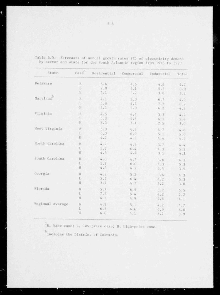
6-6

Table 6.5. Forecasts of annual growth rates (%) of electricity demandby sector and state for the South Atlantic region from 1976 to 1990

_


Delaware B 5.4 4.5 4.4 4.7L 7.0 6.1 5.2 6.011 4.1 3.2 3.8 3.7

Maryland B 4.1 3.0 6.7 4.9L 5.8 4.4 7.7 6.2!! 3.1 2.0 6.2 4.2

Virginia B 4.5 4.4 3.3 4.2L 5.8 5.8 4.1 5.411 3.3 3.1 2.5 3.0

West Virginia B 5.0 4.9 4.7 4.8L 6.0 6.0 5.1 5.611 4.7 4.5 4.4 4.5

} North Carolina B 4.7 4.9 3.7 4.4L 5.7 6.4 4.3 5.311 4.5 4.4 3.5 4.1

South-Carolina B 4.8 4.7 3.6 4.3L 5.7 6.0 4.3 5.311 4.5 4.3 3.4 3.9

Georgia B 4.2 5.2 3.6 4.3L 5.5 6.4 4.2 5.311 3.7 4.7 3.2 3.8

Florida B 5.7 6.5 3.2 5.5L 7.5 8.4 4.2 7.211 4.2 4.9 2.6 4.1


#B, base case; L, low-price case; 11, high-price case.

bIncludes the District of Columbia.

!

o_ _ _ _ _ _ _ _ _ _ . - - - - - _ _ . - - - -

|

6-7

Table 6. 6. Forecasts of annual growth rates (%) ofelectricity demand by sector and state for the

East South Central region from 1976 to 1990

State Case # Residential Commercial Industrial Total

Kentucky B 6.3 4.5 5.9 5.6L 7.0 5.6 7.6 6.9E 5.7 4.6 6.5 5.8

Tennessee B 4.3 8.0 5.2 5.1L 5.2 11.1 '.3 6.8/

11 3.7 7.9 5.7 5.2

Alabama B 4.5 7.8 4.9 5.3L 5.7 10.4 7.5 7.511 4.1 8.2 5.6 5.6

Mississippi B 4.1 6.1 4.8 4.9L 5.9 9.5 7.2 7.311 2.5 4.7 4.6 3.8

Regional average B 4.7 6.3 5.2 5.2L 5.8 8.7 7.4 7.1H 4.1 6.2 5.8 5.3


,

6-8

Table 6.7. Forecasts of annual growth rates (%) ofelectricity demand by sector and state for theWest South Central region from 1976 to 1990

.


Arkansas B 4.4 3.5 5.5 4.6*

L 5.8 5.3 6.2 5.9H 2.5 2.5 5.6 3.8

Louisiana B 3.5 3.9 3.0 3.3L 5.0 5.5 4.5 4.9H 0.7 2.0 2.2 1.7

Oklahoma B 3.5 3.6 4.8 3.9L 5.5 5.9 6.0 5.8H 0.1 1.1 4.0 1.8

Texas B 4.7 4.3 4.7 4.6L 6.0 6.2 5.6 5.9H 2.0 2.3 4.2 3.1



i

_a.

. _ _ .

i

6-9

Table 6.8. Forecasts of annual growth rates (%) of electricity demandby sector and state for the Mountain region from 1976 to 1990


Morre3na B 5.3 7.1 3.2 4.5L 5.4 7.6 3.3 4.711 6.4 7.1 4.1 5.2

Idaho B 7.1 5.8 4.2 5.6L 7.4 6.0 4.4 5.911 7.7 5.8 5.0 6.2

Wyoming B 8.2 5.5 3.7 5.5L 8.3 6.1 3.8 5.711 9.2 5.5 4.6 6.1

Colorado B 9.0 6.2 4.8 7.0L 9.3 7.1 5.1 7.511 9.6 5.1 5.2 7.0

Neu Mexico B 5.9 5.3 3.8 5.1.

L 6.7 6.7 4.4 6.111 5.9 3.5 3.8 4.4

Arizona B 10.7 7.8 4.4 8.2L 10.9 8.4 4.9 8.611 11.4 7.3 4.9 8.5

Utah B 8.2 5.6 3.9 6.2L 8.3 6.1 4.0 6.411 9.1 5.3 4.7 6.7

Nevada B 9.6 7.9 2.7 7.5L 10.0 8.7 3.4 8.111 10.1 7.0 2.7 7.4



_ _ . __ _ _ - - _ . _ _ = . _ . - - - - -_

'

!

6-10

i ;

J

[

:

Table 6.9. Forecasts of annual growth rates (%) of electricity demandby sector and state for the Pacific region from 1976 to 1990


Washindton B 3.7 5.4 2.4 3.5L 3.9 5.5 2.5 3.6H 3.7 5.3 2.4 3.4

Oregon B 3.4 10.1 4.1 5.7L 3.6 10.2 4.2 5.8H 3.3 10.0 4.0 5.6

California B 3.1 6.0 3.0 4.2L 3.7 6.7 3.2 4.8H 2.3 5.3 2.7 3.6


f


.

O

i

, __ .- -- --

__ - -. - _ _

--

|

l6-11'

!.

model are generally higher than those forecasted by NPA and usedpreviously in the Version I model. For example, the average annualgrowth rates of real per capita income for 1980-85 forecasted by BEA are4.87% for New ilampshire, and 5.71% for Florida while the comparableestimates by NPA were 3.1% and 2.2%, respectively. Furthermore, the

assumptions on fuel prices are markedly different. In general, much

higher fuel prices are used in the Version II model, as compared withVersion I. Ilowever, fuel prices affect only part of electricity costs.

As a result, dif ferences in the assumptions of electricity costs betweenVersion I and Version II are smaller in magnitude than the differencesin the prices of substitute fuels. For example, the assumed growth rateof the real price of residential natural gas in Ohio is 5.04% for 1980-85in the base case, which is almost five times the growth rate cf 1.09%used in Version I. Ilowever, the corresponding nominal growth rate ofaverage total electricity cost is 7.03% for 1980-85 which is onlyslightly higher than 5.37% assumed for the previous forecasts obtainedin Chern et al. A much higher rate of increase in the prices of subiti-tute fuels than that used in Version I would, of course, result i_n anigher demand for electricity if the estimated cross-price effect issignificant.

The validity of the forecasting results presented here are thussubject to the validity of the assumptions used. Interpretation of

these results should consider these assumptions when forecasts are1

,

4

icompared with the earlier results produced by Chern et al. It should be

pointed out that the intent here , merely to develop some uniform and |comparable scenarios for every state and to show what the model canproduce. In actual case-related work, we generally focus on one stateat a time. The assumptions of exogenous variables are each carefullyexamined based on different sources of projections. Thus, the sensi-tivity analysis is usually broader than is done here. The users of the

model'can alter the assumptions as they desire.The important findings based on these state-level results (Tables

6.1 through 6.9) are suumarized below:

1. As evidenced by the results, the forecast demand growth variesconsiderably among states for the 1976-90 period. In the residential

_ _ ,

. .. - - - . __. _ _ . - . - _ - - - -

(

6-12

sector, the forecast annual growth rates in the base case range from 1.9%

in South Dakota to 10.7% in Arizona. The forecast annual growth rates i

|of commercial demand for the same period vary from 2.8% in Illinois to

10.1% in Oregon. The base case results for industrial demand range from2.4% in Washington to 8.3% in North Dakota. As previously noted, theseresults are crucially dependent on the assumptions used. Additionally,

when comparing forecasts by state, relating the growth rate to just one

or two explanatory variables is difficult in some cases because of the

large number of these variables. I!owever, in other cases, major reasonsfor these regional differences can be identified. For example, theextrenely low growth of electricity demand in the residential and commer-cial sectors predicted for South Dakota and Illinois is mainly due to afairly low population growth projected for these states. The high

growth predicted for electricity demand in Arizona is primarily attri-butable to high projected growth of both population and number ofhouseholds. In evaluating the role.tively low growth of industrial

demand projected for Washington,-we observed that the historical trend

of industrial demand in this state registered some peculiar year-to-yearfluctuations (e.g., it had a decrease of 15% from 1957 to 1958, a 16%increase from 1959 to 1960, and a 14% increase from 1968 to 1969). This

peculiar historical pattern makes it extremely difficult to predict itsfuture demand with much statistical certainty. Fortunately, this type

,

of uncertainty occurs only in a few states. Generally, we found theforecasting results reasonable and explainable in terms of the assump-tions used and demand clasticities estimated in the econometric model.

2. In considering the three alternative price scenarios, we expectthe low-price case to result in a higher demand and the high-price caseto yield a lower demand than the base case. We found that this phenom-

,

enon generally holds for most states in all sectors because the sum of

. cross-price clasticities is smaller than the own-price elasticity,llowever, it may happen that the prices of substitute fuels increase at a

rate higher than electricity costs and that cross-price clasticities arelarge; in that situation, the high-price case may yield a demand forelectricity which is' higher than the base case demand rather than loweras one would expect. This occurs in several states.

L_ . _ , - . - _ - - -- ---

6-13|

|

For example, in Colorado, there exists a strong interfuel

| substitution in both the residential and industrial sectors which yields

I a higher rate of demand growth in the high-price case than is predicted

in the base case. However, the projected growth rates of commercial

demand follow the usual pattern among the three scenarios. As a result,

the projected annual growth rates of total demand are the same for the

high-price and base cases. The same proclivity for interfuel substi-

tution exists in the industrial sector of the West North Central region.

We find that the high-price case yields the highest rate of demand for

every state in that region. Similarly, several states, in the commercial

sector, display the substitution effect. However, the residential

sector manifests the usual pattern of demand among the alternative price

scenarios. The result is a majority of the states having a higher rate

of total demand in the high-price case in this region. For most sectors

and states, a comparison of alternative scenarios clearly shows that the

model is sensitive to underlying assumptions.

3. Comparing the projected annual growth rates for the three

sectors, we found that, in the more industrialized states such as those

in the New England region and Ohio in the East North Central region,industrial demand tends to grow at a higher rate than residential and

commerciti demands. For most other states, commercial demand for

electricity exhibits a higher growth rate than either residential or

industrial demand during the 1976-90 period. The higher growth rate in

the commercial sector is partially due to the stronger interfuel substi-

tution in this sector (the cross-price elasticity is generally more

significant and has a larger magnitude than that estimated for the other

two sectors).Tables 6.10 through 6.13 provide a summary of forecast demands by

region and for the United States for the three alternative scenarios

respectively. For the United States as a whole, total electricity

demand in the base case is projected to increase from 1804 x 109 kwhr

in 1976 to 3333 x 109 kwhr in 1990. In comparison, higher fuel prices

as assumed in the high-price case would reduce the projected electricity

demand to 3169 x 109 kwhr, and lower fuel prices in the low-price case

would increase electricity demand to 3831 x 109 kwhr in 1993.

- _ _ _ _ _ _ _ . __ _ . _ _ _ _ - - __ __. -____ __ _ _ _ _ _ _ _ _ _ _ _ _ _ _ _ _ __ _ _ _ _ _ _ __ _ -_. _ _ _ _ _ _ _ _ - _ _ _ _ _ _ _ _ _ _ _ _ _ _ _ - _ _ _ _ _ _ _ _ _ _

Table 6.10. Forecast electricity demand by sector and by region for the base case

9(10 kwhr)

1976 actual 1985 1990Region Res. Comm. Ind. Totald_ _ _ Res. Comm. Ind. Totala Res. Comm. Ind. Totala

New England 28.0 21.1 19.9 70.8 37.3 29.7 27.4 96.8 44.9 37.5 35.4 120.8

Middle Atlantic 73.3 63.0 88.7 236.8 101.8 99.3 125.4 342.9 121.3 133.5 160.5 435.9

East North Central 105.6 73.0 149.9 341.0 145.4 102.5 205.2 469.9 165.5 118.4 252.2 555.9

West North Central 48.4 29.9 40.5 122.9 65.8 51.4 65.7 189.2 75.1 66.0 87.4 236.3

South Atlantic 119.6 77.4 99.7 306.6 183.2 118.6 143.1 459.5 233.5 155.6 176.7 584.3#

East South Central 57.4 25.3 79.2 164.5 87.1 44.9 123.9 260.2 108.5 58.8 160.1 332.9

West South Central 70.9 52.5 90.5 223.0 103.1 79.9 131.9 328.0 128.0 92.2 165.5 401.5

Mountain 27.4 28.0 30.1 89.6 58.1 49.9 43.2 158.4 88.8 68.7 52.0 219.7

Pacific 79.8 68.2 88.4 248.5 108.0 119.6 111.0 356.0 125.9 165.1 133.4 446.1

United States 610.4 438.4 686.9 1803.7 889.8 695.8 976.8 2660.9 1093.5 895.8 1223.2 3333.4

" Includes miscellaneous categories.

b Includes estimated electricity demand of the DOE uranium enrichment plant in Portsmouth, Ohio.#Does not include estimated electricity demand of DOE uranium enrichment plants in Paducah, Kentucky,

and in Oak Ridge, Tennessee.dDoes not include Alaska and Hawaii.

,

I

..._ . __

.

_ _ _ _ _ _ _ _ - _ _ _ _ _ _ _ _ _ _ _ - _

.

Table 6.11. Forecast electricity demand by sector and by region for the low-price case

9(10 kwhr)

1976 actual 1985 1990Region Res. Comm. Ind. Totald Res. Comm. Ind. Totala Res. Comm. Ind. TotalG

New England 28.0 21.1 19.9 70.8 43.9 37.9 28.0 112.6 57.5 52.1 36.5 149.7

Middle Atlantic 73.3 63.0 88.7 236.8 109.2 111.9 127.0 365.7 133.5 154.8 163.4 474.4



South Atlantic 119.6 77.4 99.7 306.6 209.2 137.7 151.6 515.0 281.5 190.7 194.7 6ES.7

h#

East South Central 57.4 25.3 79.2 164.5 96.9 56.4 148.7 307.0 125.7 81.6 215.2 429.4


Mountain 27.4 28.0 30.1 89.6 58.4 53.6 43.5 163.1 92.2 75.5 54.0 232.6

Pacific 79.8 68.2 88.4 248.5 117.1 126.6 113.0 369.9 134.0 176.2 136.8 470.0

United States 610.4 438.4 686.9 1803.7 979.7 782.4 1052.3 2922.0 1252.9 1058.6 1379.8 3831.0

# '

Includes miscellaneous categories.

bIncludes estimated electricity demand of the DOE uranium enrichment plant in Portsmouth, Ohio.

#Does not include estimated electricity demand of DOE uranium enrichment plants in Paducah, Kentucky,and in Oak Ridge, Tennessee.

dDoes not include Alaska and Hawaii.

. _ _ _ _ _ _ _ _ _ _ - _ _ _ _ _ _ _ _ _ _ _ _ _ _ _ _ _ _ _ _ _ _ _ _ _ _ _

Table 6.12. Forecast electricity demand by sector and by region for the high-price case

9(10 kwhr)

1976 actual 1985 1990 -

Region Res. Comm. Ind. Total Res. Comm. Ind. TotalG Res. Comm. Ind. Total"C

New England 28.0 21.1 19.9 70.8 34.4 27.2 26.9 90.7 38.8 32.6 34.4 108.5

Middle Atlantic 73.3 63.0 88.7 236.8 96.3 100.0 115.0 337.5 111.7 136.6 159.7 428.2



South Atlantic 119.6 77.4 99.7 306.6 170.3 108.8 138.4 431.0 207.5 136.2 166.9 526.8 y'c ~

East South Central 57.4 25.3 79.2 164.5 82.8 45.4 132.1 264.6 100.6 59.0 173.3 338.4 *


Mountain 27.4 28.0 30.1 89.6 62.6 46.7 46.3 162.9 96.8 63.1 56.4 226.7

Pacific 79.8 68.2 88.4 248.5 104.2 112.4 109.3 342.4 118.6 153.6 130.7 423.0

United States 610.4 438.4 686.9 1803.7 831.1 667.5 982.0 2574.8 983.7 839.4 1230.2 3168.6

"Ireludes miscellaneous categories.bIncludes estimated electricity demand of the DOE uranium enrichment plant in Portsmouth, Ohio.

#Does not include estimated electricity demand of DOE uranium enrichment plants in Paducah, Kentucky,and in Oak Ridge, Tennessee.

dDoes not include Alaska and Hawaii.

-. -

!

Table 6.13. Forecast annual growth rates (%) of electricity demand by region,alternative cases, 1976-1990

,

Base case High-price case Low-price caseRegion Res. Comm. Ind. TotalC Res. Comm. Ind. TotalG Res. Comm. Ind. Totald

New England 3.4 4.2 4.2 3.9 2.4 3.1 4.0 3.1 5.3 6.7 4.4 5.5Middle Atlantic 3.7 5.5 4.3 4.5 3.1 5.7 4.3 4.3 4.4 6.6 4.5 5.1East North Central 3.3 3.5 3.8 3.6 2.6 3.3 3.5 3.1 4.2 4.5 5.1 4.7West North Central 3.2 5.8 5.6 4.8 2.7 6.6 7.5 5.6 4.1 6.6 5.6 5.3South Atlantic 4.9 5.1 4.2 4.7 4.0 4.1 3.7 3.9 6.3 6.6 4.9 6.0

#East South Central 4.7 6.3 5.2 5.2 4.1 6.2 5.8 5.3 5.8 8.7 7.4 7.1 i'

wWest South Central 4.3 4.1 4.4 4.3 1.6 2.1 3.9 2.8 5.8 6.0 5.5 5.7 "

Mountain 8.8 6.6 4.0 6.6 9.4 6.0 4.6 6.9 9.1 7.3 4.3 7.1

Pacific 3.3 6.5 3.0 4.3 2.9 6.) 2.8 3.9 3.8 7.0 3.2 4.7United States 4.2 5.2 4.2 4.5 3.5 4.7 4.3 4.1 5.3 6.5 .1 5.5

" Includes miscellaneous categories.b Includes estimated electricity demand of the DOE uranium enrichment plant in Portsmouth, Ohio.#Does not include estimated electricity demand of DOE uranium enrichment plants in Paducah,

Kentucky, and in Oak Ridge, Tennessee.dDoes not include Alaska and Hawaii.

.

4

b

6-18

Table 6.13 shows the forecast annual growth rates of electricity

demand by region and for the United States for the three scenarios.

There are also considerable variations of projected annual growth rates

of electricity demand among regions. However, tLe regional variation is

much smaller than the state-level variation discussed previously, espe-

cially for the total demand. The base-case projection shows th'at annual

growth rates of total electricity demand range from 3.6% in the East

North Central region to 6.6% in the Mountai:. region. For the United

States as a whole, we forecast the annual growth rates of total elec-

tricity demand to range from 4.1% in the high-price case to 5.5% in thelow-price case. The base-case projection is 4.5% for the 1976-90 period.

The forecasts of total electricity demand in the United States for the

three cases are also shown in Figure 6.1.

.

|

|

!

li

|

,

_

_

!l

' 6-19

OL |L- DWG 80-10433

| |

6,000

LOW-PRICE

BASE CASE4,500 _

_

O~

x-

.c

st:x

HIGH-PRICE3,000,

l

1,500

1976 1980 1985 1990 1995 2000

YEAR

Fig. 6.1. Forecasts of U.S. electricity demand, 1976-2000.

.

_ _ _ _ _

|

!'

I

i

7 CONCLUSIONS

This report presents further results of validating the Version I

model, an investigation of structural change, an update of the Version Ii

| model as Version II, the electricity cost forecasting model, and the

forecasts of electricity demand and prices by sector and by state for

1977-2000.

Further validation of the Version I model was conducted through

ex post forecasting in the post-sample years of 1975 and 1976. Generally,

the ex post forecasting errors are smaller for residential demand than

for commercial and industrial demands. One reason for higher errors for

comoercial and industrial demand forecasts is due to the reclassification

of customers between these two sectors. Furthermore, the ex post fore-

casting results reveal no evidence of any significant non-price induced

conservation in 1975 and 1976. The estimated price elasticities appear

to capture reasonably well the consumers' responses to changes in elec-i

tricity prices during recent years.

An update of the Version I model was made to incorporate additional

data for 1975 and 1976. This updated model was referred to as the

Version 11 model. In the course of updating the SLED model, potential

structural changes were investigated. The statistical results, however,

show that changes in either the general structure of the denand equations

or the estimated own-price clasticities between Version I and Version II

of the SLED model are generally not statistically significant. Even

though, in most cases, the same specification used in the Version I

model is retained in Version II, the use of more data during the post

oil embargo period would enhance the credibility of the SLED model.

A new set of the assumptions of exogenous variables was developed

and used to forecast electricity demand and price by sector and by state

for 1977-2000. It should be stressed that forecasts made with econ-

ometric models are only probabilistic and contingent on the validity of

the assumptions used. A broader sensitivity analysis than the three

fuel-price scenarios presented in the report can be conducted with the

SLED model developed in this study.

7-1

_ _ - _ .

7-2

The forecast rates of growth in total electricity demand vary

considerably from state to state: Arizona has the highest rate (8.2%),

and Massachusetts and Illinois have the lowest rate (2.9%). Furthermore,

electricity demand is found to be sensitive to changes in the prices of

fuels and costs of generating, transmitting, and distributing electricity.

For example, in the New England region, doubling the rates of growth for

all fuel prices and electricity costs in real terms would reduce total

electricity demand by 10.2% in 1990, and by 18.8% in 2000. In some

regions, however, the impacts of increasing the prices of substitute

fuels, especially natural gas, offset that of increasing electricity

costs. As a result, the net effect on electricity demand resulting from

increases in prices of fuels (high-price scenarios) is positive rather

than negative.

In our continuing efforts to refine the SLED model, we are currently

involved in developing what will be called Version III of the SLED

model. In this version, the model is split into two separate but relatedI

components. The first determines short-run utilization rates conditioned

upon the saturation of electric appliances, and the second estimates the:

saturation of appliances. Sevecal recent studies have focused on theimportance of modeling short-run durable use decisions and longer-rundurable choice decisions at the micro level. Our work focuses on aggre-gation in such models and further considers issues in specificationwhich enhance possibilities for greater breadth of application.Preliminary regression results for the short-run usage equation in theresidential sector show that the saturation of important electric

appliances affects both the aggregate own-price elasticity and the

aggregate demand for electricity.

|

|

|;

i

|,

.

|

|

FOOTNOTES AND REFERENCES

1. W. S. Chern, R. E. Just, B. D. Holcomb, and H. D. Nguyen, RegionalEconometric Model for Forecasting Electricity Demand by Sector andby State, ORNL/NUREG-49, Oak Ridge National Laboratory, Oak Ridge,

Tenn., October 1978.

2. Ref. 1.

3. W. S. Chern and R. E. Just, " Regional Analysis of Electricity

Demand Growth," Energy, forthcoming.

4. R. S. Pindyck and D. L. Rubinfeld, Econometric Models and EconomicForecasts, McGraw-Hill, New York, 1976.

I 5. L. R. Klein, A Textbook of Econometrics, Prentice-Hall, Inc. ,

! Englewood Cliffs, N.J., 1974.

6. G. S. Gill and G. S. Maddala, " Residential Demand for Electricity

in the TVA Area: An Analysis of Structural Change," Proceedings oftk, Business and Economic Statistics Section, American Statistical

Association, Washington, D.C., 1976.

7. M. Allais, "A Restatement of the Quality Theory of Money," American

Economic Revico, 56: 1124-57 (December 1966).,

1'

8. In 1976, total fuel costs for all privately-owned nuclear power

plants in the U.S. were estimated at 467 million dollars while total

generation costs were 902 million dollars. See footnote 11 for,

data sources. |!

9. D. L. Phung, Cost Competitiveness Between Base Load Coal-Fired and j

Nuclear Flants in the Mid-Term Future (1985-2015), Institute for

Energy Analysis, Oak Ridge Associated Universities, May 1976. Note

that Phung's estimate was based on pressurized and boiling water'

reactors.

,

R-1

|

i

R-2

10. Ediscn Electric Institute, Statistical Yearbook of the ElectricUtility Industry for 1976, Edison Electric Institute, New York,1977,

11. Federal Power Commission, Statistics of Privately Ouned ElectricUtilities in the United States,1976, U.S. Government PrintingOffice, Washington, D.C., 1977.

12. Federal Power Commission, Statistics of Publicly Ouned ElectricUtilities in the United States, 1976, U.S. Government PrintingOffice, Washington, D.C., 1977.

13. The utility file which is referred to as the Generating UnitReference File, was originally compiled by the Federal Power

f1Commission (FPC), and has been taken over by FERC in DOE. ORNL

has maintained and updated its own version of the file,

14. U.S. Department of Energy, Energy Information Administration,t

Annual Report to Congress 1976, Volume Three, Supplement One,

DOE /EIA-0173/3-S1, U.S. Government Printing Office, Washington, fD.C., July 9, 1979.

15. Ref. 1.

16. Bureau of Economic Analysis, U.S. Department of Commerce,

" Population, Personal Incom'e, and Earnings by State, Projections to2000." Regional Economic Analysis Division, October 1977.

17. Bureau of Economic Analysis, U.S. Department of Commerce, Survey of

Cherent Business, Vol. 59. No. 8 part II, U.S. Government PrintingOffice, Washington, D.C., August 1979,

18. Data Resources, Inc. , U.S. Forecast Swamary, Lexington, Massachusetts,November 1979.

19. These projections were obtained from Dr. Terry Morlan, Chief,Demand Analysis Division, Energy Information Administration, May1979.

_ __ _ _ _ . _ _ _ _ _ _ _ _ _ _ _ _ _ _ _ _ _ _ -

R-3

20. Ref. 18.

21. National Planning Association, Regional Economic Projections:

| 1960-1990, REPS Report No. 76-R-1, Washington, D.C., June 1976.|'

22. American Gas Association, Cas Utility Industry Projections to 1990,Washington, D.C., September 1976.

23. Energy Information Administration, U.S. Department of Energy,Annual Repont to Congrass 1976, DOE /EIA-0173/S-S1, U.S. Government

Printing Office, Washington, D.C., July 9, 1979.

24. Ref. 23.

25. Ref. 1.

26. Ref. 1.,

o

,

:

11

.

O

- - _

_ - - _ _ _ _ _ _ _ _

Appendix A

EX POST FORECASTING ERRORS, 1975 AND 1976

o

.

<

.

g. - - , - - _- _ . -

A-3

- - . -

W W F F F W Ww4e@OC eedmA99 P ee 84 ae wCN(ON -Coppo -epmehwegamy w e. e == *= -e eam-cr h p =.? O hoere h e p == e*= 0 0 h == hereoaPeeoe ge e e ee ge e e ee aeeeoe 30 e*** CP e e* e 20e*eoC =s m b - E Dan c O O @ C-ereN O==#eed C--N-N C= temp O-cehmC ===e*** a a == t , a N N - fs C es'e a i eI t c * I==* E e I i

R I 1 E e E f 9 e1 R E R ' E6 ene h 4 h b b

> e. > > > e- >r er e e s* r rgeetee eepeme are e se r o e ce6meO yo. 0. e e N40.pog e r =.e p p

pe. c r at ==ergoeg ymppog

w"*mMEEV Un* O N m e ve= e m W O va.gmng@ eeoe sureeoe her o e o e beoee e w?eee* WP e e* = w9eeee

%Q G se r k N e O mo t h m @ G ae O e == - G as e M m e 3-ONO- B == p h "'I O G == e C M eh C ---- Q - d i I C NNNN C t i l 5 C t ti s C 1 1-= C ee e

b 1 89 6 b k I i 14 6 4 k I i bgP"4

*t3C

e eOOrc sc=e- c m $NNNpe. O.m m O@ see-c e.Noep e. e e r.rg

oogo m e, o m y h opO gh. em e. g c 0p e e er hcecoeeoee p * eee ee eae p eoe eeoee eeeo e Pee e*O == e o P P =ec1pO =e o h e er == p h e. ( == e m e r, == e == m G == m r e r

N mm-A eeNe emNM een, eeme geme erne@

lu b b k W 4 kH v w w w==

6

** Ce. a. as

w ve.-

e R C c C Dg &Odekt 4 0 8.e e O C c == Fe == D a ce- p N r C,#PPet afehNA Cee-(F

Aemec Achre hep-O hbere A me. Ahome kmkhry.J9 e e o e JOeeeo seeee JPeeee Jeoeee J&oeee JP e o e e

@ e-C600 4-ee90 e-peen 4 -t- e a& P e-emer e ==e A m o e == == A c F4 3 m m h et 3 veNF 3 mmMM 3 geme 3 eene 3 eeme 3 OONe

> > > > > > >g w w v v v v we 4 e 4 e e 4

ksoO ecteN e e e p en erNm e, gem e g e gy p eejece erhcr

h m e k sf h00@@ ab h O @ P- heNNN A r == G P- *= W O @ == ** e r == rT3 ee ooe oe o *e toeoe yeeee eeeee ee oe e peeoeC == = =* e 6 -iPM= ==O m N C =en == = e - p O N :o =OeeC ** @ e = C

mm-N mmNF mmNN ggmm eeme enNm eeN"g

kOUU

- - - -y - -

e n n u a w *a we e e e == wePe*N wommemm we N M *t r see. m =.o r we. c h e @==@ O -r P

pmeNem o =e m harpp h ey r o g e gemm e O@6 ** m e m ==>g e oe RFeeoegpeeoe areoee apee ee gpesea ge ea,p e o e eC =e s* O N O Caertr e e O=e m efs D=em@me Cas t- e *= b O-4&Nm Oas e c O P-,Q

d D I t e e f 4se a se * r eeee e seee g e e i a e s == a' E O & R C Q R *

W ar tu w he b w ald ' ' * * * * *O e e r e r e rH ece e c at eceOO- erhe=0 eeeece wee pe ecNm-r ecmeONla uh-=mh uhmepe wh-peh vorehm wheee- wh0Nes ve* N c O e

eoe tup e * e eg g2P e e e o tu sip e e oe esp e oeo e tap e e e.o. tp0.=e. O c -esse..oa - eO.e eeo

e=ees g. n=ePNre=cNON CC - O *= O f - O O - O e *= r a.

C * e i O ===# > 0 - t 2 O I e I ea C 6= a C tt **N 6 I L k w b I e h 3 L 6 hC e e- J u

-w e r -

Cr

I = *I >y e T U U CWk 1 O e w b >

y .2m y e c 7so e a seee a seee + .cee O sooo 2 e e .o n .es.

e eeNen 6, es--e e6 ch006 e e-hkr 1 ee%-e a emmme w epsee@ E hpNeC Z mmOE. > heOre I hm@he c kNe#4 V h@-Ob Z AeO@A

PaOeN p e e {t rP ** p o'l e p h Pe@@O pere- p & e m. (54 -viOm@e

wee eOve

C C 0 C .. =O h O-Ns e.es =r -- m . e. .O = et .= N #1 N E

C O C2- Z Z 2 Z Z z

y e e e e e e ez s a z x y aD k eeea m eeoe ts eoea w eeee g; eoee su oeoe es, eee*

D 00 @ * O =) De == O - N Of O e ** m DekDee Oppmer ce m e == O Oc *- O == E4 h-fmo hecOO hheeN heer beh-T hhNpp hoh-r

so.-ee s em peh m Je*-ehsemm- Jo-eca Jeecce g am - m.Ne . Oh g- =e e .= > p t c 4 *= g O h 4g e= N eo h e eseN es e e-- g-N 3 3 3 3 -- N 3 3 - 3 NaNrN > > > > > > >u o y v v v U4 e e 4 4 e e

* eeee eeee e ose e eea seee eeee e**e4 4 0 * *= 9 e N m ** ss emem e OeO e m p == N e c N == r s p ea r **

.e.e c s N h.e. N o.s heo=< hpmNre-Oe-O h--ep hecNN.eeme pe cc peohepehmO e-ech pecee eye-cy

oO- n =

-here-N-Ne -N -e . - - n -Opra ----e =n.rerP4 ANNr

@E*

.i. e. d did did .d .i. a $diddi .s. -ii de. e. . - e --=.

*USJ e v a es e-vgJ >va J >vaJ e-WEJ >VRJG20=e CFE*4 EFced E20=d 22Emd C7G>d 22D==c an k t* * Cwdr* Ciu w @ * Ceewea C iss w V * C4wer O to b e *->O33D aOf3C eCf3C -OID *Cf3C =cz3C *0230

U,{S*u Me= .u En> u., g c e= U-{c> w-C2U-pO> U-FO>

m rto w W.r

We weuz or r vz we@ lna v == e tu W -r tu W = e4 ht w == to ens W == etJ-

4 E E a a is a

n - _ - _____ _ _ _ _ _ _ _ _ _ _ _ _ _ _ - _ _ _ - - _ _ _ - _ _ _ _ _ - _ _ _ - _ _ _ _ _ - _ - _ _ _ _ _ . __ __ _-

a

,

Table A. -(continued).NEW J3RSEY

SECTOR 4974 AC IU Ahf SO L MA ND. FORE C AS I ENHOM (t) AC T U At Ph4CE F OHf C AS T E RNUR (t)

t 1976 497S 19F0 1974 89FS '1976 1975 8976prSIDENTI AL B424s. 34S76. 35090. -2.84 *l.94 44 57 49.2S S2.71 ~6.9F -9.S4

C 0e ME HC I AL 32904. 33550, 34289. -34.83 -9.05 42.08 4E.02 48.26 -F.09 -6.74INDUS TRI AL $6 59 5. 14928. 4S759. 0.29 -4.84 28 89 Jt.79 33.85 -0 26 0.96

TOTAL 43543. 43084. 4S438. -S.24 ~5.23 37.$2 421 T 44.4F -S.F3 -S.81

PENNSY&WANIA

AC Yuat DEMANO - PnaECASI ERHOH dat ACIUAt PHICE FGHECASE ERROM (ElSE C TOR 3 9F4 99FS 19F6 1975 89F6 89F4 89F5 19F6 897% 1976

bE SI DENT R AL 26673. 27724 28790. 0.22 06S JS. 28 39.96 41.20 -82 57 -82.84(CM MF RC I AL 16338 I TIS 9. 17892. 4.74 ll.13 33.e6 J6.34 3F.98 -82.82 ~84.38$ NDUS T RI AL 44 F 86 4838F. 43366 -0.FF -F.44 28.04 25.33 25.F2 -88.66 -47.F0

TOTAL 87797 86200. 90048. 0.65 -1.17 27.3d 32 23 33 38 -14.F0 -13.85

DHiQ

ACTUAL DEMAND FOef C A ST tHWOR 43) AC T U AL P R I C E" F OR F C AS T ENht p (si

SECIOR 1 974 39FS 1976 1975 5976 8974 89FS 1976 89FS 39F6RE1 f 0ENT I AL 26747 20020. 289S2. ~2.6S -8.68 29.00 34.s 2 35.64 -S.33 -9.22

( OM ME RC 8 AL 18878 38879. 3959%. -3 39 -0.36 27.69 32.54 33.F5 -4.20 -6.68t m0UST R I AL 49648. 4SS24 S2158. 0.67 -7.36 15.78 89.52 89.3F -0.82 4 40

TOTAL 94S43. 92423. 800 FOS. -1.53 ~4.30 21.82 26.60 26.84 -3.83 -3.9F

INOBANA

ACIUAt DEMAND FORECAST ERROR (t3 AC T U AL PutCE F Ou t C AS g tuhou tsp ASEC TON 3 9F4 89F5 1976 697S 1976 89 F4 39FS 1976 89FS 1976

& E S I DE N T I AL 44668. IS998. 36S96 l.42 3.49 24.38 26.69 30.20 ~6.42 -82.26C OM MFHC l at - 79F2. 895S. 9283. -l.80 S.05 24.24 26.56 29.40 -6.16 -9.50I ND US T R I AL 23642. 21980. 246SF. -0.01 -3.53 84.26 37.95 19.94 -85.64 -85.45

T O T AL 46275. 46926. SOS 34. 0.82 0.30 89 86 22.57 25.03 -9.FF -12.86

ILLINOIS

ACluAL DEMAND FOWECAST ERRDN 83) AC TU AL PN!f E F OH E C AS T (Rwoq 83)

SE C TOR 1974 197S 89F6 8975 8976 19F4 89F5 8976 19F5 8976RF S IO* NT S AL 240SS. 26192. 26325. -4.82 1 83 32.46 35.63 38.S8 ~1.60 -4.7F

C OMMCRCI AL 20S67. 284SF. 22443. I.S6 2.32 30.15 34.92 37.64 -S.tS -6.38I ND US T R E AL 32289. 33389 33345. -8.S2 -50.37 86.35 20.37 22.49 0.28 -3.02

TOT AL 76984. 79038. 82409. - 4. 32 -3.28 2S.08 29.18 38.F9 -1 49 -2.90

MICHIGANn

ACIUAL O k MA ND FONECASI EHWOR (t) ACTUAi PhlCE F OR E C AS F E R hf M 419SEC TOW B 974 89F5 1970 19 FS 39F6 19 F4 3 9 FS 1976 8975 89F6

RE S IDE NT I AL 20289. 20807 24345. -0.43 -l.34 29.66 35.35 38.88 -3 34 -6.43C Cae ME RC I AL 82648 12949. 1346S. 3.tF 0.90 30.01 36.2F 40.26 -4.69 - 8.38I ND US T R I AL 29036 2 F OS F . 38067. -at.SF -12.55 89.04 24.80 2F.03 -S.3S -4.79

T O T AL 68902. 60813. 6S877. -S.0S -6 3F 24.75 30.85 33.57 -3 32 -S.tl

u8SCONSIN

ACTUAL u tim A ND FORECAST ERNUM 453 ACTUAL PNBCE F OutC AS I thkoM 443SEC TOR 9 9F4 89FS 1976 99F5 89F6 8974 8975 89F6 197S 59F6

RE S IDENT I AL 48299. II904. 42377 -2.F8 -2.90 27.30 38.35 34.37 7.66 4.95C OMME RC S AL 6 86 F. 7685. 824S. -81.90 -9.82 28.78 32.33 33.89 7.98 9.60INnuSTRI 4 1822F. 806St. 188F6 I.70 -0.02 57.15 21.00 23.45 BS.28 IJ.30

TOTAL 29392. 30869. 3t798. - 3.50 -3.e8 2J.77 27.94 30.40 9.03 8 09

i

- -- 0 1 - - - m _____.._j

._._--__ _ .. . _ . . _. . _ . . ._ _ - . _ _ . . . .

,

Table A. (continued)DELAsANt

AC T U A E DEMAND FONFCASI ENROh (El AC.fuAt PHICE tONFCA51 thMOR (t)SECTOR 8 9 F4 39FS 39F6 1975 59F6 8974 19FS 1976 19FS 19F6RS S I DF NT I AL 1482. 8483. 3S64. -S.34 -S.42 40.82 43.50 46.26 ~4.69 -F.14

C O4 MC RC I AL 8522. 3864 1883. =9.F6 -F.69 37.83 40.04 45.35 -F.0S -8.22- I MO US T RI AL 28FO. 2484 2632. S.F3 - F. 4 F 25.S8 29.30 28.98 -6.52 -3.53

TOT AL S404 5833. SJ F 9. -0.93 -6.92 38.96 35.84 36.40 -F.0$ -S.88

M ARYL ADe0 A as0 D. C.

AC1UAL D E MA ND FOREC45i ERkDR EE) AClud' PR I C f. F ONEC AST ERNGH 448SECION 8 4F4 19FS 19F6 197S 89F6 49F4 49F5 4976 8975 8976

RESIDENTSAL 30020. 50 SOS. 10994. -88.$8 -80.3F 35.84 39.49 40.55 20.34 17.93C og aeE R C I AL 9900. 10469. 10864 -88.80 -80.94 35.8F 38.47 48 29 20.56 53.96I ND US T R t AL 32048. ISSS8 83469 -3.49 -t F.6 F 23.36 26.68 25 25 36 .6 9 4S.82

TOT AL 38968. 32532. 3S327 -9.FS -33.33 38 85 34.61 34.94 24.28 24.FS

*VIRGINI&

ACIUAL DEMANO FOMECAST ENHOR tal AC TU AL PRICE FONECAST tRHON (t)SECIOR 3974 49FS 3976 8975 3976 1974 197S 1976 4975 49F6

e f s t DE NT I AL. 84559. 85450. 866F0. -S.42 -7.0F 28 25 34.52 35.08 ~4 23 -4.65C OM ME R C I AL 9544. 10342. 40990. -8.69 -6.96 2F.2F 33 99 34.23 -6.66 -S.01I ND US T RI AL 900F. 8 F4 S. 96 72. 6.05 -4.59 58.24 23.35 22.89 -1.05 8.77

TOTAL 33880. 3453F. 37332. -3.49 -6.40 25.23 38 53 31 67 -S.14 -3.F2

WE$f wf*eGINIA pACTUAL DEMAND FORECAmi ERROR (t) AC T U AL PRICE F OREC AS I E N HE W7 (t)

SEC TON 1974 1975 89F6 89 FS 1976 1974 5975 1976 8975 4976RE$ 4 0ENI B AL 4$42. 4862. S328. -3.68 -3.44 27.23 32.F0 JS.85 -S e l ? -9.94

( CM esE RC I AL 2 e 4 3, 2848. 3023. -3.46 -3.23 26.69 31.29 34.23 -F.62 -18.79IMOUSTRI 4. 9950. 98S7. 9906. 9.29 -3.66 15.24 20.78 2 4.8 B -L4.47 -82.89

TOT 4L 4F13S. 36867 68050. 3.40 -3 53 20.03 25.99 27.87 -88 89 -St.SS

N. AND S. C AROL lNA

Aslual DEMANO FORECAST ENROR 458 AC T U AL RRICE F DH E C A$ T EhMOR (atbE C lON 8974 8975 89F6 49FS 89F6 1974 1975 8976 19FS 89F6

DE SIDE NT 8 4L 2 F 323. 28843. JOSIF. -3.69 -S.28 25.30 29.3F 32.98 0 50 -S.34( 04 Mf pC I AL ISF49. 16979. 3 F98 3. -8.66 -F.94 23 14 27.29 29.6F -2.98 -S.2SI ND US s R g At 31686. 3 20S 3 < 3S244 S.46 -6.62 B4.82 89.40 20.55 3.0t S.tS

TOTAL F6FSS. FF8FS. 84044. -l.00 -6.45 20.26 24.82 27.06 -0.52 -l.98,

e GEOGGRA

AC l u a t. OEMAND FGdECASI ENNUN 450 AC1UAt PRICE F Ok & C AS T ENNOR (t)SECIOR 8974 1975 8976 8975 B976 89 F4 1975 49F6 8975 8976

NESIDENIRAL IS4Fl. I6409 1846F. -6.03 -40.40 23.02 28.14 29.33 3.8F 2.56C re ME RC I At. 10625. 48099. 42889. -6.08 -9.68 26.83 34.09 35.62 -6.05 F.8 3INJu$1R5AL 64093. 8 3 50 F . 84590. S.38 -3.69 16.08 23.23 23.CF -4.F8 -0.96

T OT AL 40te9. 480lS. 45246. -2.28 -8.02 21 69 28.13 29.00 f.49 -2 28

FLOHIDA

FOWi(5ASI EHROR 633 ACTUAt PHICL F Ow erC oh l ERh0H 413ACluaa OkMANDht C ION 397 19F5 19 F6 197 1976 IwF4 1975 1976 l % F5 1976

. RF SiO8 nil AL 33329. 34627 JS969. -2.99 -0.81 28.42 34.38 L6.65 2.64 0 25i C G4 MF NC B &t. 58935. 20520. 21283. -6.68 -4.20 30.SF 36.15 3 F.8 2 1.37 2.S2

IN0us f Rt AL 01370. 13615. 84885 2.49 Belt 88.09 24.00 2!.06 8.78 4.B4T O T at 6S657 68762. F3367 -2.98 -I.45 27.80 32.F8 3S.09 2.68 3.93

|

,

Table A. (continued)asl NN* hul A

As t u tt McMANO tuM CAST tNh04 Esp ACTUAt .*W I C E FOHtCAST ERh0M (t)se c tos. 1974 19FS 8976 3975 1976 8914 89th 19 F 6 4G75 19F6

NF S IDE NT I AL 9 596. 30089. 406S2. 8.92 0.63 27.84 J 0. 9 3 33.29 4.39 2.94(neur wC I AL 4t50. 4436. 4884. 2 98 I.74 10.46 32.48 35.37 -2.89' -2.00I ND UG I R I AL 80969. 88024 18 5 F6. ' l.25 -0.58 17.30 25.32 2 J .6 b -0 8F -3,00

TOTAL 24 SIS. 2beF9 27348. 1 80 0.33 23.61 27.21 29.43 4.S3 -0.03

t

Susa

AC lu At UEMAND FORECASI ERRUw (t) At1UAL PHICE F OH e!(. 4S I LRNON 848SEC thR 1914 89FS 3976 1975 8976 tvF4 1915 1976 1975 1974

P F 5 8 0F N T I R F63S. 8226. e462. -2.74 0.07 28.78 32.66 36.30 2.08 -0.86C OM ME R C I AL 4208 4622, 4848. = $ . 70 0.81 28.83 33.6 4 36.80 -S.54 - F. 4 BINDUSThiAL 6746. 6660. 7866 8.16 4.36 85.74 89.90 22.24 -4.28 -3.68

TOTAL 18 SS9. 39508. 20446. 0.75 8 75 24.07 28.56 31.48 -2.74 -3.44

MISSOURI

ACTUAL DEM4NO FOMEC4ST ERROH 42) ACTUA6 PRICE F OW F C AS I LhMOR ttlSEC TOR 19 F4 89FS 3976 1935 4976 1974 49FS 49F6 1975 8976

NE SIDENT I AL 4 8 F D6. 83032. 33532. -S.6% -0.59 28.S5 38.6 1 35.33 2.46 -1.02C OM 4E RC I AL 6987 F479. FFOS. 0.20 4.3F 2F.28 30.59 34.45 -l.86 -S.4FI ND US T RI AL 18242. 18079 19882. l.F8 -1.48 16.99 20.48 23.55 -2.88 ~4.34

TOT 4L 2986S. 38650. J3839. -0.66 0.24 23.90 2'.40 30.82 -0.46 -2 95

NORIH 044014'

OAC IU AL GEM 4NO FOkEC4ST ENDOW (%) ACTUAt PR IC C F OW tC AS I tRHow Ett

SECION g 9 74 1975 8916 B975 8976 8914 89FS 1976 39FS 1976RE S I DE N T I AL 5668. 8763. 3995. F.37 0 39 26 39 28.65 30.8 3 -80.FS -80.72

C OM ME R C I AL . 1013. ll23. 8 26 F. 0.22 -1 58 23.9S 26 87 28.50 -4.75 -6.67INDUSTRt4 494. S59. 632. 3B.SS 16 02 25.84 25.36 26.69 -88.37 -te.64

TOftL 3154. J 44 5. 3894. S.76 2 18 24.93 2'.31 29.40 -10 85' -10.34

SuufH DAAOTA

AC T U A 0 DEMANO FG ut C A S T ghROR (43 ACTUAL PRECE PORECASI LRROH 4%)SECluH 3 9 F4 8975 19 F6 39FS 3976 4974 1975 4976 8975 8976

RE S I DFN T R A&. 8847 1964. 2334. 0.B6 *4.no 26.26 28.02 33.58 30.34 8.lFCOMMERC8AL 965. 1023. 3423. 0.39 -2.F8 28.42 38.02 34.58 -2.30 -3.92I ND U$ f R I AL 458. 48 3. 493. 6.85 85.S9 87.48 89.03 21.58 F.96 lo.FF10TAL 3263. 3468. 3750. 3.14 -l.10 25.69 27.65 33 53 S.65 3 67

!

NERD 4 SEA

AC IU AL DEMANO FONECASI ERROR (El AC T U AL PRICE' F OH t C AS T ERNOM ltlSer TOM $ 9 74 397S 8916 8975 19F6 49 F4 59FS 39F6 8975 8976

RE s t 0EN T 8 AL 4 2SS. 4635. 4837. -3.49 -l.83 22.49 25.40 29.51 13.65 8.94C OM M F HC I AL 3S42. 3F74 4012. B.99 3.84 19.33 22.61 26.SF B2.03 7. F4INDUSTHSAL 2290 2345. 2673. -2.26 -6.89 83.88 IS.Ft 18.60 24.37 88.50

TOTAL 80093. 10804. 48542. -8. 30 -1.S6 89.26 22.28 25.95 .34 17 10.36

KANS45

AC I U At. DEMAND FUWECAST EkHnu tal AC TU AL PRICE FOHECabi ERNUR (ElSECTON 0974 1915 8976 975 89F6 5974 5915 19F6 8975 4976

hfSIDENTIA6 S839. A58 3. 6768. -S.29 -1.44 24.73 28.83 3883 4.53 2.8BCOMufRCIM. St&S. SFFF. 6888. -2.28 2.16 22.02 26 82 29.50 7.54 F.26I ND US T R I AL SSSR. 5 b8 6 . h826. 6.80 8.84 43.42 87.80 20.52 3.38 2.67

TOTAL 86S83. I '7 8 F 6. 88782. -0.54 2.94 20.08 24.58 27.56 4 25 3.58

_ _ . _ _ _ _ , _ - _ _ .

_ _ _ __

_ _ _ _ - .__ - _ - - _ - -

Table A. (continued)a FNY UC M Y

ACTUAL DEMANn FORCCAST ERROR (El AC T U AL #R if F r nR EC at t FRRS atSEC TO8t 1974 49F5 19F6 8175 1976 19 74 89F5 1976 19FS ..Is)

PF SIDFNT I AL 9433. 80098. 10728. -2.36 ~5.tF 21.60 24.44 26 24 2 15 6.07C OM ME DC I AL 7940. 8F30. 30238. -0 88 -20.It 84 28 35.59 86 68 23 84 15.76INDUSTRI AL 135tF. 33FJF. IF025. - 0.95 -85.95 13.69 39.58 20 68 - 25.4 F -85.34TOTAL 10090. 32565. 3F994. -3 32 -84.01 16. 30 20.02 2 8. l F -4.88 3 46

7 ENN T S SE E

ACTUAL DE MA ND FORECAST ERROR ft) AC T'I AL RRI(F F OR EC AS T FRROR ttiSECTOR 1974 1975 1976 8975 4 9 F6 89F4 8975 1976 8975 1976R E S I DE N T I AL 24693. 22467 23636. -a.,*s -F.85 85 65 20.69 23 00 -6.35 -0.00C04MERC3AL 3ete. 3672. 3887. -g..- -g.68 19.72 25 02 PF.19 3 02 2.3FI NO U11 R t AL 39469. 30843, 33999. S.8F -4 82 18.04 37 20 49 8 F -82 85 -54 83TOTAL M6780. 96292. 68522. l.0M -9.93 83 15 39.30 28 09 -9.48 -9.3F

ALARAMA

AC TU AL D E MA ND FORECAST ERROR (El ACTUAL PRICF F OR EC AS T FRROR ttiSE C TOR 8974 19F5 1976 4975 4976 1974 89F5 8976 89F5 4976# F S I D* N T I AL 13828. 43953. 14768. -5 4F -3.92 20.89 25 15 2F.S8 ~6.4' -30.31C 04 ME RC I AL 574F. 6204 6486. -9.69 -6.F6 24 33 28 34 30.25 -8.98 -9.A5INDUSTRtAL 23044 21320. 24826. 6.38 -5.6F 12 20 3 T. 6 2 18.38 ~4.53 -3.12TOTAL 48982. 48277 45380. 0 82 ~9 26 16.MS 28 92 23.04 -F.3F -F.84

MtSSISSIRRE >|

ACTUAL DEMAND FORECAST ERROR (23 ACTUAL PRICE FfRFC AS T ERRnR tt)$?C TOR 8 9 F4 89F5 1976 39F5 1976 5974 89FS 8976 8975 59F6# E S IDENT I AL F363. 7868. 823F. -9.S2 -7498 23.30 25 17 38 32 13.72 1.80C OM ME R C I AL 4034. 4388. 4784 -82.62 -16 2S 25.48 27 82 33 53 22 4 F 2.68I N3 US T RI AL 6698. 6525. F23 F. 3.05 -5.02 16 39 20.25 23.88 6.89 4.72TOYAL 58095. 18738, 20888. -6.5S -8.85 25.15 23.90 29 05 10 20 2.19

ARKAN949

ACTUAL DEMAND FORECAST EPROR (El AC TU AL PRlrF r tm EC AS T F#ROR tttSEC TOR 1974 1975 89F6 19F5 19 F6 89F4 1975 1976 1975 19F6RE SI DENT I AL 5F25. 6356. 6703. -8.89 -9.76 26.35 29.25 33.94 12 55 6.69C 04 4F RC I AL 3389. 3 81 F . 4084. -6.68 -4.23 25 35 2T.50 32 24 11 73 5.6%INDUSTRIAL F063. 5895. 6489. 48.80 -88.50 15 58 86.42 22.F2 82 34 -F.0810TAL 36877 4 5 3A 9 172F6. 8.81 -9.18 29.44 24.4h 29 32 6.94 2.83

L OUI 4 8 AN A

ACTUAL DFMAND FORECAST FRROR (t) ACTUAL #ptrE F OR EC A'. T FRROR Etl$*C TOR 8 9F4 8975 1976 19 F5 19F6 1974 1975 49F6 197S 89F6R E S I DE N T I AL 58649. 82536. 13373. -2.8F l.48 24.63 24.86 26.F0 IF.33 IF.85C E4 MERCI AL 6845. F689. 8829. -3.63 0 21 23.90 24.62 27.S2 14.37 8.53I ND US T R I At., 1F360. LF146. 19535. 4.46 -8 32 12.48 12 65 13.29 19 5 F 26.5FTOTAL 15454. 37308. 4803F. 0. 34 -3.46 13.60 19.20 2 0. 4 R 35 90 19.72

Ou t.46F144

AC TU A L OFMANO FORECAST F pA OF (49 ACTUAL PRiff F ORFC AS T FRROR (4)SEC TOR 3 9 F4 39F5 39F6 l9 75 1976 19 74 8979 19F6 39F9 89F6#F SIOFNT I AL 8086. 8945. 9407 0 46 4.34 23.93 25.67 29.93 6 0F I.94CC44FRCIAL 5729. 6346. 6532. 3 38 4.03 20 8% 22 32 26 24 5 04 0.93INDUSTRIAL 6463. 653J. F385. 6.08 -3.86 II.28 83.59 1 F.6 3 7.58 -I.93TOTAL 20209. 78624. 23824 2.54 8.70 IR.'4 FI.0F 29.07 M.4F 1.67

_ _ _ _ _ _ _ _ _

-- _ _ _ _ . _ _

11

Table A. (continued)TEyA9

ACTUAL OEMANO FORECAST FARQG (1) AC TU AL PR if F ronECAST FRDDR stbSECTOR 1974 1975 1976 49 FS s9F6 19F4 50F% 8976 19F5 89F6

eE ? I DE N T I AL 37849. 40390. 41423. 2.59 88 85 24.07 27 30 31 36 6.17 6.F6

C 09 4E SC R AL 30809. 323F8. 33F23. 2.E" 5 58 20. 75 24.24 27 65 3.84 4.8B

INO US T p t 4L S2448. 5 2 24 J. 5 FJ39. 5.76 -3.78 88.56 84,88 88.48 6.22 8.46

T O T AL 120405. 324608. 132479. 3.90 3 27 17.79 29 30 24.Fm 9.50 '6.26

MONTANA

ACTUAL DEMANO FORECA%T FOROR lti ACTUAL PRICF rnp f C A% f EmpDR (tl

SECTOR 19 F4 19F5 8976 1975 8 9 F6 49F4 I4F5 $9F6 1975 89F6

p* SIDE N T I AL $677. 2038. 2232. -0 09 -3 87 22 30 23 92 22.34 3.30 0.59

( C#'*F OC I AL I498. 1544 1669. 80.FF ll.5F 20 45 20.8F ?O.62 -5.07 -4.91

I ND US T RI AL 5963. 5089. SF95. 89.9F B6.35 S.03 6.28 6 09 80.F9 17 08

TOTAL 9929. 8673. 9696. 83 62 30.R' 10.96 12 52 12 33 -1 0 T 0.im

IDANO

ACTUAL DEMAND rOoEC49T ERROR (El ACTUAL PRICF F OR EC AS T ERROR ltlSEC TOR 19 F4 19F5 1976 1975 8976 1974 89F5 1976 1975 19F6

R E S I DE N T I AL 3393. 3788. 4804. -0.90 -1 83 15.6' 36.44 18.14 2.33 -l.88

C D4 m E R C I AL 3298. 3292. 3517 3 56 0 13 84 06 86 01 I F.9 0 2.8m -1.98

I NO US t e l As_ 5556. 9540. S547 24 58 35.47 6 90 8.55 80 86 -3.20 -8.62

TOTAL 8216F. 12620. 33869. II.45 I4.48 II.24 12.R6 14.78 -2.49 -R.29

y. 7. N c.M

ACTUAL DEMAND FOeECAst EpnOq ft1 ACTUAL pp I C f' r OD EC as t EppOn Ett

SEC TOR 1974 3975 3976 59F5 8976 19F4 8975 89F6 1975 1976#E 5 8 DE NT I AL 785. 464. 970. 4.04 2 59 23.79 23.67 24 84 F.46 8.R4

C O4 ME RC I AL 1443. 1513. 8730. 16 07 9.83 86.90 I F. 3 3 87.F2 9 31 13. F I

INDUSTRIat 1835. 1966. 2006. 21.50 24.82 10.F0 30.R9 82.02 8.48 8.4F

T OT 4L 4063. 4348. 47m6. 85.96 84.90 15.43 15.69 16.%4 6.75 8.19

COLOBADO

4C T U AL DE MA NO FORECAST ERROR Ett ACTUAL PRICF r on E C AS T EppOR (43

SEC TOR 8974 1975 19F6 1975 1976 1974 19F5 89F6 49F5 49F6

PESIDENF I AL 4F49. 5095. 5361. 2.94 3.38 27 53 31.04 12 64 ~1 3 2 -2 26

C rM ME #CI AL 5864 6296. 62F3. 4.55 12 18 22.42 25.83 28.69 -I.69 -6.09

I NO U5 t RI AL 3809. 3335. 4820. -3.52 -12 09 84.20 17.98 59.24 -7.52 -8.4F

TOTAL 13722. 34726. 15F%4 2.87 2.82 22. 32 29.F7 27.56 -1 94 - 1. 6 F3

e.Eu eralCO

ACTUAL DEMANO FORECAST E#ROR lt) Arfnal Pa tr F F on Fr. AS T FPROM (ElSEC TOR 8974 8975 59F6 8975 8976 8974 49F5 8976 1975 89F6

DE SIDE NT I AL $795. 1903. 2027. 0.97 1.89 29 05 32.'l 35.93 -F.29 -10.52C ON #E RC I AL 2552. 2646. 2904. 33 63 f.96 22 48 25.25 27.69 -5.F8 -8 02I NO US T R I AL 3517. 4650. 1992. 5.24 3.84 14.F3 IF.5F 20.84 -84 35 -8F.04

TOTAL 5964 6899 6923. F.58 5.00 22.49 2M.4 9 28.05 -F.69 -10 99

ARIFONA

ACTUAL DEMANO FOGECA97 FRROR tti ACTHAL PRICr r opfC AS T Fnpne (48

SEC TOR 1974 19F5 $976 1975 5976 8914 ISTS 1076 1975 8976

RESIDENT!al 66St. 6#40. 7214. -2.56 -4.48 29.96 16.4% 39.02 -4.2^ -11.64

C O4 MERCI AL 6300. e 62 4. 6895 -8.09 -4.99 25.03 32.29 35.23 -0.06 -R.93IND U$ t pl A 5788. 5726. 60F6. 3.89 6.49 17.63 22.68 24 60 6.82 -4.05

TOTAL tmF39. 39290. Folgt. 0.76 -3.31 24.44 30 93 g 3. g p -l.40 -g 6 3

_ _ . _

Table A. (continued).UTAH,

ACTUAL OrmaNO FORgCAST FRROR (El AC T U AL PR Ir r FORECAST rppnm EttSEC TOR 8974 39F5 1976 19F5 1976 8 .~ F 4 1975 1976 1975 19F62420,'#FSIDENf84L 2520. 2683. 3.70 2 00 22.95 2*.68 31.70 -13.F7 -38.9%C C4 mE RCI AL 2054 2256. 2560. 1 2F -5 80 20.20 23.FF 26.15 -5.03 -5.82I NO U5 f p l AL 288F. 2333. 2362. -8.25 5 68 84.08 8F.0F .20 03 ~5 59 -F.84'

TOf4L 6661. 7909 7605. -0 99 0 73 89 11 22 43 2e.21 -9 93 -82.In

NEWADA

AC TU AL DEMAND FORECA57 FRROR (t) ACTUAL PRICF F OR EC A5 7 FRROR lt)SEC TOR 8 9F4 89F5 89F6 1975 B976 1974 1975 19F6 19F5 19F6

R E s t Of NT I AL 2 F94 293B. 2785. 3 73 8.39 19.79 23 55- 28.41 -0 40 -4 88C OR4ERC I AL 2524 2745. 2451. -3 92 '32.65 21 05 26.B5 30 38 0.20 -l.09IMOUSIR E AL 2808. 8756. 2 8 6 F. 22.44 -3.49 13.45 13.39 49 54 33.44 -18.38TOTAL 7426. 7332. 7403. 6 80 6.32 38.03 22 09 26.47 0 14 -3 38

WASHINGTON

ACTU AL DEuaNo FORECA57 EpDOR ttl ACTUAL ppICE F t1 REC A51 FRROR gelSE C TOR 8 9F4 1975 39F6 1975 3976 89F4 1975 8976 49F5 1976

PE 5 t OE Nil AL 19487 21088. 223B6. -t.50 -1 98 11 36 32 29 12.68 0.78 -1 0FC C4 mE RC I at. 9256. 9959, 10F22. I.42 -0.02 12 5F 13 83 84.08 -0.88 -0.48INOU$ f RI AL 2F243. 36412. 28967. 3.60 -8.01 J.J3 4.35 4.58 6.30 3.F2TOTAL Sg93g. 57392. 6200%. 4 45 -4.60 7.59 m.90 9 83 0.F2 3.F6

>neroON :

ACTUAL OFMANO FORECAST EPROR 441 ACTUAL PRICF F fief C AS T FRROR tt)?EC TOR 1974 49F5 8976 B 9 75 1976 1974 19F5 ISF6 19F5 5976

pF5tOENil4L 11565. 12246. 12489. 2.72 5.30 14.53 16.45 18.5F -9.28 -33.94( C4 mE RC I AL 6F60. FF00. 7868 0.58 5 26 34 89 te.32 3 F.22 -3 53 -2.98INDUSTRIAL 42959 12894 33628. F.F4 -2 80 4.94 6.F6 8 04 -2 . 0 F ~4.F4TOTAL 18294 32140. 33985. 4 15 2 22 10.64 82.69 14.01 -6.94 +F.47

CALIFORNIA

ACTUAL OFMANO Frl#FC457 PR40R (19 ArYUAL DRif[ . F OR EC AS T FRROR 45)SE C TOR 3 9F4 1975 19F6 1975 8976 1974 8975 e16 B975 89F6

P E S I DE N T I AL 48409. 43383. 45055. B.96 -4.49 30 79 33.35 35.42 -2 44 -3 66C 04 ME RC I AL 44739. 4e635. 495F6. =F.FI -8.22 2 F.6 3 JV.2F 33.38 -1 93 -4 03L NO US I Rl AL 43646, 42742. 45FF6. -0.94 -6.85 18.08 28 22 24 33 -0.42 -3 38

TOTAL 129793. E32 FRO. 140407 -2.40 -6.33 79.40 29.3F 18.On -3.76 -2 96

|

- ..- - . .- ..~ . . . . - . . . . - - . - - - - - - - . . - . - . - - . _ . - - . _ . - - . -_..

_-

!'ii

2

4,

.

I .

';

i

!tt.1

.

1

I

,

W

ie

1

i!

{ Appendix B1

i~j REGRESSION RESULTS OF THE VERSION II MODEL!

!

I.

t

4

i *

i

4:I

(l

1

J

J

j

.

,

4

1

i4

'

s4

,

L

4

4

6

1

E

I4

1

|

4

!

I

k

.

{:;'

.--,--..~-,.,,....--,,,-.....,,-..---..._---,_,_----...-....,_-m-,.,...--~ ,__ ..... _ _ . .. ,, - -.- -... -, - - -

- - _ . _ - - _ - _ - - - _ _ _ - _ _ _ _ - - _ . - _ . - - - - _ _ - - _ - - _ _ _ _ - _ __ _. . _ _ _ _ - _ . _ _ _ _ _ . . _ _ _ - _ _ -,

e:

Table B.1. Three stage least squares estimates of residential demand by region, 1955-1976"

Normalized variable: In ERS

In in D In in in In S In S In2

i ion Const.nt ERS (PER/ CPI) (PER/ CPI) (PC1/ CPI) In CR (POP /CR) In HDD in CDD (ICR/ CPI) (RCC/CR) RCC Rt-1

New England -3.112 0.818 -0.210 0.130 0.299 0.146 0.183 0.017 0.051 0.993(-4.77) (52.39) (-9.56) (4.20) 55.54) (2.73) (4.10) (2.22) (4.02)

Middle Atlantic -4.165 0.647 -0.218 0.015 0.365 0.639 0.318 -0.013 0.030 -0.003 0.999(-3.18) (23.63) (-9.68) (8.32) (8.09) (7.07) (4.45) (-0.36) (2.76) (-3.72)

East North Central -2.708 0.680 -0.349 0.009 0.047 0.409 -0.120 0.013 0.014 -0.002 0.996(-1.95) (14.31) (-5.33) (2.84) (0.90) (2.73) (-0.64) (0.25) (0.93) (-1.53)

West North Central -8.318 0.637 -0.254 0.0004 6.81e 6.126 0.019 0.995(-7.14) (17.28) (-4.79) (0.01) (8.67) (2.39) (1.37) go .

South Atlantic -1.035 0.723 -0.299 0.017 0.237 0.302 0.169 0.068 0.047 0.042 0.995 L3

(-1.52) (32.90) (-9.05) (5.21) (7.16) (6.93) (2.62) (4.07) (2.92) (2.48)

Last Sout5 central -6.201 0.572 -0.355 0.015 0.300 0.741 0.293 0.173 0.104 0.052 -0.001 0.996(-4.86) (10.69) (-6.96) (2.98) (4.03) (4.55) (1.65) (4.55) (3.02) (0.84) (-0.73)

West South Central -9.134 0.568 -0.392 0.172 0.s88 0.425 0.140 0.138 0.007 0.996(-5. 7 5) (10.44) (-4.79) (2.36) (5.34) (2.91) (4.25) (3.76) (0.14)

Hountain -2.963 0.627 -0.139 0.462 0.636 0.691 0.156 0.033 0.069 0.984(-3.61) (16.93) (-2.95) (5.58) (8.54) (5.92) (2.49) (2.02) (2.57)

Pacific -3.790 0.811 -0..!6 0.024 0.285 0.179 0.019 0.997(-3.03) (18.84) (~1.53) (0.35) (2.61) (4.81) (2.01)

# 2The figures in parentheses are estimated asymptotic t-ratios; R is the squared correlation coefficient between the actual andestimated values of the normalized variables; S is a dummy variable having the value of one for 1971-76 and zero otherwise; all other stateand reclassification dummy coef ficients are not presented.

. . . .

_ _ _ _ _ _ _ _ _ _ _ _ _ _ _ _ _ _

_ _ _ _ _ _ _ _ _ _ _ .. .. ... .. . . - _ _ -

B-4

Table B.2. Three stage least squares estimatesof residential price by region, 1955-1976"

Normalized variable: PER-TOC

Region Constant ERS/CR (ERS/CR)2 CR q2

New England 11.877 -5977 480396 0.00002 0.979(6.57) (-11.97) (10.04) (7.39)

Middle Atlantic 20.169 -4291 455749 0.000001 0.989'

(6.74) (-5.56) (7.18) (0.38)East North Central 14.533 -2231 137230 0.000001 0.992

(16.39) (-4.76) (4.01) (1.58),

West North Central 20.949 -3696 214437 0.000007 0.992(26.92) (-10.34) (7.44) (5.54)

South Atlantic 20.318 -2662 180408 -0.000002 0.983(20.20) (-14.63) (11.92) (-3.53)

East South Central 15.041 -1823 80669 0.000001 0.995(22.70) (-12.75) (10.98) (0.90)

West South Central 25.693 -4293 272343 0.0000004 0.994(11.51) (-15.38) (11.45) (0.45)

Mountain 10.888 -1353 58883 0.000003 0.983(10.04) (-5.08) (4. 03) (1.91)

Pacific 16.596 -838 39884 -0.000001 0.997(25.93) (-2.85) (3.26) (-2.33)

#The figures in parentheses are estimated asymptotic t-ratios; R2

is the squared correlation coefficient between the actual and estimatedvalues of the normalized variables; all state and reclassification

|- dummy coefficients are not presented.

.

.._..-min

..

Table B.3. Three stage least squares estimates of <_ommercial demand by region, 1955-1976"

Normalized variable: In ECS

In in D+1n in in in S In in

Region Cons tan t ECS (PEC/ cpi' (PEC/ CPI) (PCI/ CPI) In CC POP in HDD in CDD (PGC/ CPI) (CCC/CC) (CCC/CC) R2t-1

New England -2.209 0.805 -0.294 0.275 0.321 0.132 0.010 0.128 0.988(-1.29) (26.25) (~4.39) (3.09) (2.43) (0.94) (0.41) (2.71)

Middle Atlantic -2.831 0.402 -0.208 1.272 0.716 0.002 0.153 -0.009 0.988(-4.29) (7.09) (-2.70) (7.10) (10.27) (0.03) (3.75) (-2.64)

East North Central -0.608 0.795 -0.289 0.012 0.149 0.215 0.106 0.040 0.031 0.995(-0. 8 6) (15.27) (-2.67T (2.35) (2.24) (3.40) (1.66) (1.69) (0.51)

West North Central -2.744 0.851 -0. 72 0.343 C.037 0.006 0.988(-3.31) (25.09) (-2.89) (5.28) (1.59) (1.53)

tz

South Atlantic 0.432 0.698 -0.355 0.026 0.350 0.308 0.027 0.049 0.988 8

#(0.57) (22.82) (-6.12) (3.93) (5.06) (4.48) (0.82) (1.66)

East South Central -1.089 0.510 -0.589 0.025 0.373 0.366 0.150 0.266 -0.00089 0.966(-1.13) (8.95) (-6.39) (2.61) (3.70) (4.47) (2.68) '?.78) (-0.36)

West South Central -0.581 0.880 -0.171 -0.007 0.139 0.051 0.045 0.997(-1.92) (19.62) (-2.09) (-0.12) (3.42) (1,18) (1.02)

Mountain -5.161 0.504 -0.433 -0.019 0.976 0.033 0.972(-6.48) (12.23) (-7.18) (-2.57) (10.13) (1.07)

Pacific -14.116 0.437 -0.205 0.556 1.263 0.073 -0.257 0.992(-7.29) (10.19) (-1.83) (2.51) (8.27) (2.97) (-4.66)

"The figures in parentheses are estimated asymp' otic t-ratios; R is the squared correlation coefficient between the actual and2

estimated values of the normalized variables; S is a dummy variable having the value of one for 1971-76 and zero otherwise; all other stateand reclassification dummy coef ficienta are not presented.

.

>

_ _ _ _ _ _ _ _ _ _ _ _

l

B-6

Table B.4. Three stage least aquares estimatesof commercial price by region, 1955-1976"

Normalized variable: PEC-TOC

2Region Constant ECS/CC (ECS/CC)2 CC R

New England 11.725 -770 9648 0.0001 0.983(3.67) (-9.82) (8.86) (2.89)

Middle Atlantic 34.824 -308 6143 -0.00005 0.989(16.75) (-5.44) (6.59) (-9.58)

East North Central 14.384 -460 5284 0.00002 0.988(12.86) (-13.01) (11.61) (2.42) s

West North Central 16.086 -625 7342 0.00004 0.991(11.55) (-12.71) (7.47) (2.30)

South Atlantic 20.528 -403 5299 -0.00001 0.981(26.99) (-] .92) (14.30) (-4.25)

East South Central 15.573 305 2910 -0.00001 0.981(10.86) (-2.70) (1.49) (-0.60)

West South Central 17.491 -500 5984 0.00000001 0.995(10.88) (-12.82) (9.82) (0.002)

Mountain 12.933 -353 3146 0.00004 0.976(21.66) (-12.31) (11.14) (4.11)

Pacific 8.252 -270 2429 0.00001 0.994(10.87) (-6.97) (6.09) (3.23)

#The figures in parentheses are estimated asymptotic t-ratins; R2is the squared correlation coefficient between the actual and estimatedvalues of the normalized variables; all other state api reclassificationdummy coefficients are not presented.

.

k

m - . i._.. --_ -- - ~_ , ,- . .-

,

I

i

!

#Table B.5. Three stage least squares estimates of industrial demand by region, 1955-1976

'

Normalized variable: In EIS,

In in D*In in in S.In In D In D; * In IniRegica Constant E15 I I | ( ^I | ' I I I ^| I ~( ^| I E I

t-1

New England -0.989 0.667 -0.038 0.454 -0.007 0.921(-1.88) (18.38) (-0.52) (7.47) (-2.51)

Middle Atlantic -2.183 0.291 -0.081 0.041 0.990 -0.011 0.138 0.066 0.009 0.996(- 2. 21) (6.65) (-0.67) (3.50) (10.98) (-4.58) (2.28) (1.18) (0.35)

East North Central -0.691 0.342 -0 391 0.036 0.741 -0.012 0.089 0.096 0.977(-1.09) (7.67) (-3.04) (3.48) (13.37) (-4.36) (1.42) (4.80)

IWest North Central 0.476 0.711 -0.172 0.259 0.120 0.971(0.80) (20.44) (-1.38) (5.04) (2.15) na

South Atlantic 0.326 0.824 -0.077 0.187 0.003 -0.001 0.968 da(1.44) (32.29) (-1.44) (4.61) (0.13) (-0.68)

East South Central 0.929 0.449 -0.298 0.528 0.027 0.218 0.956 '-

(1.98) (6.90) (-2.01) (7.41) (0.27) (2.24)West South Central 0.467 0.769 -0.111- 0.223 0.045 0.962

(1.95) (17.29) (-1.69) (5.79) (1.69)Mountain 1.798 0.523 -0.201 0.374 0.067 0.919

(4.46) (13.47) (-1.88) (7.95) (0.941 -

Pacific 0.134 0.606 -0.041 0.372 0.036 0.930(0.22) (10.51) (-0.46) (4.81) (1.99)

,

"The figures in parentheses are estimated asymptotic t-ratios; R2 is the squared correlation coefficient between the actual and

estimated values of the normalized variables; S is a dummy variable having the value of one for 1971-76 and zero otherwise; Dg isthe state dummy for New York; D2 is the state dummy for New Jersey; all other state and reclassification dummy coef ficients are notpresented.

e

_ _ _ _ _ _ _ _ _ _ _ _ _ _ _ _ _ _ _ _ . _ __ ___ _. - _ _ - -

_ _ _ _ _ _ _

i

|

|

B-8

Table B.6. Three stage least squares estimatesof industrial price by region, 1955-1976"

Normalized variable: PEI-Tor

Region Constant EIS/CI (EIS/CI)2 CI R2

New England -8.656 1.915 0.661 0.001 0.959(-4.38) (0.99) (0.87) (4.28)

Middle Atlantic -3.078 6.365 -1.668 -0.0001 0.974(-2.38) (3.07) (-1.89) (6.33)

East North Central -1.359 -0.412 0.044 0.00005 0.965(-2.84) (-1.20) (0.68) (1.79) 1

West North Central -7.305 6.986 -2.532 0.00037 0.974(-9. 40) (6.57) (-5.68) (6.13)

South Atlantic -5.770 2.165 -0.292 0.0001 0.931 I(-9.93) (3.47) (-2.39) (4.04)

East South Central -5.081 3.841 -0.719 0.00015 0.949(-8.33) (4.69) (-3.70) (3.34)

West South Central -10.925 11.569 -5.680 0.0002 0.951(-7.78) (4. 94 ) (-4.32) (5.50)

Mountain -14.685 1.141 -0.030 0.0005 0.971(-10.19) (5.83) (-5.15) (5.04)

Pacific -3.065 0.210 -0.014 0.00001 0.995(-18.47) (2.17) (-1.58) (4.33)

#The figures in parentheses are estimated asymptotic t-ratios; R2

is the squared correlation coefficient between the actual and estimated

values of the normalized variables; all state and reclassification dummycoefficients are not presented.

|

t

.

!

|

||t

1t

!

i

Appendix C

FORECASTS OF ELECTRICITY COSTS

.

4

%

s

,-y , y ey -- . .r4 ,-yv-

._ . _ . -- - m. . . . -_ ._. _ .m _ .m, _ _ _ _ _ _ . _ . _ . _ _ _ ___ _._ . . __ _ _ _ . _ _ _

SSSES C .T. A CT U A L (1976) . AND ASSOMED SHARES OF POWER GENER ATED BY OIL, COAL, AND GAS [T)

1

OIL COAL CAS

. STATE 1976 1980 1985 1990 1976 1980 1985 1990 1976 1980 1985 1990

ME- 100.0 100.0 100.0 64'.7 0. 0 0. 0 0.0 35.3 0.0 0.0 0.0 0. 0NH 45.7 47.5 47.5 47.5 54 3 52.5 52.5 5?. 5 0.0 0.0 0.0 0.0 ,

YT 67.7 67.7 67.7 67.7 25.4 25.4 25.4 25.4 6.9 6.9 6.9 6.9

MA 99.3 '97.8 97.8 97.8 0.0 1. 6 1.6 t. 6 0. 7 0.6 0.6 -0.6

RI 90.5 90.5 90.5 90.4 0.0 0.0 0.0 0. 0 9.5 9.5 9.5 9.6 .

C7 99.7 99.7 99.7 99.7 0.1 0.1 0.1 0.1 0. 2 0.2 02 0.2

MY -78.3 .78.7 77.6- 76.4 21.0 20.6 21.7 22.9 0.7 0.7 0.7 0.7

NJ 64.7 :64.8 65.0 65.0 31.0 30.9 30.6 30.6' 4. 3 4. 3 4.4 4.4

PA 9.9 10.1 10.1: 10.1 90.1 89.9 89.9 89.9 0. 0 0. 0 0.0 0.0

CR 18 1.8 - 1. 8 18 97.9 97.9 97.9 97.9 0.3 0.3 0.3 0.3

: IN 1. 3 13 1.9 19 98 2 98.3 97.7 97.7 0.5 0.4 0.4 0.4

IL - . 7. 4 8.2 8. 5 . 8.9 89.1 89.4 88 1 87.8 3. 5 3. 4 3.4 33MI 15.1 16 1 15.4- 15.4 70.6 78.7 79.6 79.6 5. 3 52 5.0 5.0

WI 2. 5 3.1 3.0 30 93.7 93 3 93.5 93.5 3.8 1. 6 1.5 3. 5MN 5. 4 5.2 4.8 4. 8 89.1 89.5 90.3 90.3 5. 4 5.2 5.0 5.0

In 3.9 4.7 4.5 4.5 82.4 82.4 83.0 83.0 13.7 12.9 12.5 12.5M0 2. 0 ' 2.8 3.5 3.5 93.2 92 5 92.0 92.0 4.8 4.7 4.5 4.5

MD 16.8 16.8 16.6 16.6 81 0 R t.1 81 3 81 3 2. 2 21 21 21'

SD 3.2 5.4 5.4 5.4 94.3 92 1 92 1 92 1 26 2.5 2.5 2. 5 nNB 14.8 13 4 12.5 12 5 60.5 64.6 66.7 66.7 24.6 22.1 20.9 20.9 8

"+

KS 17 1 16.6 15.6 15.6 31 1 34.0 38.1 33.1 51.7 49.4 46.3 46.3'

DE 67.8 60.8 60.8 61 1 33.6 35.7 35.7 34.0 3. 6 3.5 3.5 34MD 49.8 49.6 50.6 50.9 43.4 45.6 48.6 43.3 0.8 0.8 10.8 0.8

TA 51 1 51 1 51 1 51 1 48.8 48.8 48.8 48.8 0.1 0.1 0.1 01-WV 0.6 0.6 0.6 0.6 99.4 99.4 99.4 99.4 0. 0 0.0 0.0 0.0

NSC O. 8 10 1.0 10 99.2 99.0 99.0 99.0 0. 0 0.0 0.0 0. 0GA 11.7 11.5 12.6 12 4 87.3 87.6 86.5 86.7 10 0.9 0.9 0.9 *

, FL 66.0 65.9 65.0 64.5 18.5 19.0 20.3 21.0 15.5 15.1 14.7 14.5'

FY 02 0.3 0.3 0.3 99.8 99.7 99.7 99.7 0. 0 0.0 0.0 0.0

t TN 2. 3 23 23 23 97.7 97.7 97.7 97.7 0.0 0.0 0.0 0.0

AL 0. 8 0.8 0.7 0.7 98.4 98.4 98.5 98.5 0.8 0. 8 0.8 0.8'

MS 54.3 51.6 50.1 47.5 26.7 30.3 32.4 35.9 19.0 13. 1 17.5 16.6AR 80.2 71.9 55.7 55.7 0. 0 10.3 30.6 30.6 19.8 17.8 13.7 13.7LA 17.6 17.7 17.1 16.5 0. 0 0.7 3.8 7.8 82 4 81.6 79 1 75.7

CK 0. 6 0.9 0. 7 0.7 0. 0 3. 3 7.9 7. 9 99.4 95.8 91 4 91.4 r

TI 1. 7 1.7 1.8 1.3 10.1 12.6 15.8 16.4 88.2 85.7 R2 4 81.8,.

FI 0.8 0.7 0.6 0. 6 97.4 97.6 98.0 93.0 1. 8 1.7 14 14ID 11 1 11 1 11 1 11 1 0. 0 0. 0 0.0 0.0 88.9 88.9 89.9 88.9

WY 0. 4 0.5 0. 4 - 0.4 99.3 99.3 99.4 91.4 0. 3 0.2 0.2 0. 2,

! CO 33 32 31 29 76.5 77.7 78.9 79.5 20.2 19 1 18.0 17.6*

i NM 3.1 3.0 2.9 29 66.1 67.5 69.1 63.1 30.R 29.5 29.0 29.0AZ 18.4 18.2 17.7 17.7 69.6 70.6 71.5 71 5 12.0 11 2 10.8 10.8

1

itt 0.8 0.8 0.6 0.6 91.8 92.9 13.9 93.9 7. 4 6.3 5.5 5.5

NV 7.9 2.9 2.7 26 77.5 77.7 79.9 80.0 19.6 19.5 18.4 17.4,

UA 0. 3 0.4 0. 4 0.6 99.7 99.6 99.6 99.4 0.0 0.0 0.0 0.0

CR 100.0 100.0 16.6 16.6 0.0 0.0 83.4 83.4 0.0 0.0 0.0 0.0

CA 67.0 67.2 67.3 67.5 0.0 0. 0 0.5 0. 5 33.0 32. 8 32 2 32.0

<

-- - - - - - _ _ _ - _ _ - _ _ . - - . _ - _ - _ - _ _

- - _ . _ . - _ _ _ -- .. , . . . ,, - - -_ - ,- - . - . . . . . _ - ..- - -. ~-

TABLE C.2. LCTULL (1976) 49D ASS 0MED SH ARRS CF POWER G2NEP ATED BY STEAP, E1CLTA3, AND HYDRO ?L4NIS [9)

Sif45 N1 CLEAT HYD70---

E

ST4TE 1976 1980 1985 1990 1976 1980 1985 1990 1976 1980 1985 1990

ME 11.7 11.7 11.7 17.1 65.4 68.6 63.6 64.4 23.0 19.7 19.7 18.5MM -73.0 73.7 57.8 57.8 0.0 0.0 21.5 21.5 27.0' 26.3 20.7 20.7VT 1.0 1. 0 1. 0 10 75.4 77.1 77.1 77.1 23.6 21 9 21.9 21.9M4 87.6- 97.8 86.1 82.8 11 1 10.9 12.7 16.0 13 13 12 12

' RI 99.4 99.4 69.9 69.9 . 0. 0 0.0 29.9 24.9 0.6 0.6 0.3 0.2CT 47.5 47.2 47.2 47.2 50.9 51 3 51 3 51 3 1.6 1. 5 15 1.5NY 59.4 58.8 57 2 56.4 14.4 15.7 17.9 18.6 26.2 25.5 24.9 25.0MJ 94.9 80.7 75.4 72.0 15.1 14.3 24.6 28.0 0.0 0.0 0.0 0.0P4 84.5 83.6 81.2 80.7. 14.3 15 2 17.6 17.5 12 12 1. 2 18

1..OH 100.0 99.1 96.7 95.3 0.0 0.9 3. 3 4.7 0.0 0.0 0.0 0.0IM 99.2 99.3 96.7 96.7 0.0 0.0 2. 6 2.6 0.8 0. 7 0.7 0.7IL 73 1 71.7 69.5 6 8. " 26.8 28.2 30.4 31.0 0.1 0.1 0.1 01

i MI 84.5 83 1 81.3 81.3 14 2 15.6 17.5 17.5 13 13 12 1.2

| WI 65.6 66 2 65.3 64 2 30.5 29.9 31 0 32.2 3.9 3. 9 3. 7 3.5i 1N 63.7 64.6 66.0 66.0 34.7 33.3 32 4 32 4 1.7 16 16 1.6

I4 82.6 83 3 79.9 79.9 13.8 13.2 16.8 16.8 3.6 3. 4 32 3.290 98.2 98 1 95.3 95.3 0.0 0.0 30 3.0 1.8 1.9 1.8 1.817 43.9 44.9 45.2 45.2 47.2 46.4 46.1 46 1 R.9 8.8 8. 7 8. 7S3 29.6 30.2 30 2 30.2 0.0 0.0 0.0 0.0 70.4 69.8 69.8 69.810 47.7 50.4 49.0 48.0 . 42.9 40.7 40.9 40.9 4.4 8.9 11.0 11.0 9

i KS 100.0 100.0 97.0 97.0 0.0 0.0 3. u 3.0 0.0 0. 0 0.0 0.0 e'

3E 100.0 100.0 100.0 100.0 0.0 0.0 0.0 0.0 0.0 0. 0 0.0 0.090 79.1 77.3 77.6 7 3. e 16.5 17.4 17.2 21 3 5.4 5. 3 5.2 4.9'

YA 76.8 74.5 69.7 67.9 20.9 23 1 24.4 26.4 2.3 24 5. 8 5.7WV 99.4 99.4 99.4 99.4 0.0 0.0 0. 0 0.0 0.6 0. 6 0.6 0.6MSC 86.7 84 2 93.8 79.9 4.1 7.0 7.6 12.0 9.2 8. 8 8.6 8.1G4 81.7 81 4 79.0 79.3 8.9 9.6 11.5 11.4 9.4 9.1 9. 4 9.3FL 89.1 88.4 87.5 87.6 10.6 11 3 12 2 12 1 0.3 0.3 0.3 03

*KY 94.5 94.5 94.9 95.0 0.0 0.0 0.0 0.0 5.5 5.5 5.1 5.0 ,

TN 84.3 79.9 73.0 73.0 0.0 4.4 12.5 12.5 15.7 15. 8 14.5 14.5<

At 75.0 72.9 71.5 71 5 7.7 10.3 12.3 12 3 17.3 16.8 16.2 16.2MS 100.0 100.0 83.5 84.2 0.0 0.0 16.5 15.8 0.0 0. 0 0.0 0.04R 51.8 52 3 59.7 58.7 31 6 32 7 29.4 28.4 16.6 15.0 13.0 13.0LA 100.0 10 0.0 96.3 96.4 0.0 0.0 37 3. 6 0.0 0.0 0. 0 0.0OK 95.6 95.8 94.3 92.7 0. 0 0.0 18 3. 4 4.4 4. 2 3. 9 3.9

' TI 99.3 99.3 97.7 97.4 0.0 0.0 17 2.0 0.7 0. 7 0. 6 0.69T 22.7 23.5 26.8 26.8 0.0 0.0 0. 0 0.0 77.3 76.5 73.2 73 2ID 01 0.1 01 0.1 0.0 0.0 0.0 0.0 99.9 99.9 99.9 99.9WY 93.4 93 6 94.0 94.0 0.0 0.0 0.0 0.0 6.6 6. 4 6. 0 6.0CO 92.9 91.9 9 ?.1 92 2 0.0 1.0 10 1.0 7.1 7.1 6.9 6.8N1 99.6 99.6 93.6 90.6 0.0 0.0 0.0 0. 0 0.4 0. 4 0.4 0.4

' 42 71.3 72.6 68.8 67.1 0.0 0.0 51 7. 4 29.7 27.4 26 1 25.5UT 72.3 75.3 76.9 76.9 0.0 0.0 0.0 0.0 27.7 24.7 23 1 23.1M7 89.0 39.0 89.5 90 1 0.3 0.0 0. 0 0.0 11.0 11.0 10.5 9.9v4 6.0 6.~ 6.2 6.1 23 2.9 5. 5 6.7 91.7 90.7 88.4 87.109 0.0 02 0. 9 0. 9 5.6 5.6 5. 5 9.1 94.4 94.2 93.6 90.0C4 76.1 73.5 72 3 71.7 41 72 8.0 9.1 19.8 19.3 19.6 19 2A7G. 71 8 71.5 69.2 68.8 12 1 12.7 15.4 15.9 16.1 15.8 15.4 15 2

- _ _ _

-

99968 f 1. ASSUMED GRO3TH R ATE OP OIL, CO AL, AND GAS PRICES (1)

OIL COAL GAS- _ -

=- _ _ . - - - - - - - - - - - - - - - - - - - - - - - - - - - - - - -

4

STATI .1976-1980 19EO-1985 1985-1990 1976-1980 1980-1985 1985-1990 1976-1980 1980-1985 1985-1990

ME 12 20 11 20 6.50 5.60 4.60 6.50 11.60 10.60 7.10NH 12 20 11 20 6.50 -5.60 4.60 6.50 11.60 10.60 7.10YT 12 20 11 20 6.50 5.60- 4.60 6.50 11 60 10.60 7.10MA 12 20 11 20 6.50 5.60 4.60 6.50 11.60 10.60 7 10-RI 12 20 11 20 6.50 5.60 4.60 6.50 11.60 10.60 7.10CT 12 20 11 20 6.50 5.60 4.60 6.50 11.60 10.60 7 10NY 13 10 12 10 6.40 8.80 7.80 6.70 15.30 14.30 7.20NJ 13 10 12 10 6.40 8.80 7.80 6.70 15.30 14.30 7.20PA 13.70 12 70 6.40 9.90 8.90 6.80 13.00 12.00 8.80CH 11.00 10.00 6.60. 8.20 7 20 6.30 14.50 13.50 10.20IN 11.00 10.00 6.60 8.20 7.20 6.30 14.50 13 50 10.20IL 11.00 10.00 6.60 8.20 7 20 6.30 14.50 13.50 10.20MI 11.00 10.00 6.60 8.20 7.20 6.30 14.50 13.50 10.20WI 11.00 10.00 6.60 8.20 7.20 6 30 14.50 13.50 10 20MN 11.00 10.00 6.60 8.20 7.20 6.30 14.50 13.50 10 20IA 12.80 11 80 6.70 7.30 6 30 5.20 18.70 17.70 6.80MO 13.00 12.00 6.60 8.70 7.70 6.10 17.60 16.60 9.80 jND 12.80 11.80 6.70 7.30 6.30 5 20 18.70 17.70 6.80SD 12.80 11. 90 6.70 7.30 6.30 5.20 18.70 17.70 -6.80 mMB 13.00 12.00 6.60 9.70 7.70 6.10 17.60 16.60 9.80 f,KS 13.00 12.00 6.60 8.70 7.70 6 10 17.60 16.60 9.80DE 13.70 12.70 6.40 9.90 8.90 6.80 13.00 12.00 8.80MD 13.70 12.70 6.40 9.90 8.90 6.80 13.00 12.00 8.80VA 13.70 12.70 6.40 9.90 8.90 6.80 13.00 12.00 8.80WV 13.70 12.70 6.40 9.90 8.90 6.80 13.00 12.00 8.80MSC 13 30 12.30 6.70 10.50 9.50 6.30 16.20 15 20 8.70GA 13 30 12 30 6.70 10.50 9.50 6.30 16.2u 15 20 8.70FL 13.30 12 30 6.70 10.50 9.50 6.30 16.2v 15.20 8.70KY 13.30 12.30 6.70 10.50 9.50 6.30 16 20 15 20 8.70TN 13 30 12 30 6.70 10.50 9.50 6.30 16.20 15.20 3.70AL 13.30 12.30 6.70 10.50 9.50 6.30 16.20 15.20 8.7095 13 30 12. 30 6.70 10.50 9.50 6.30 16.20 15.20 8.70AR 14.50 13.50 6.60 7.60 6.60 6.00 18 20 17 20 7.00LA 14.50 13.50 6.60 7.60 6.60 6.00 18.20 17.20 7.00CK 14.50 13.50 6.60 7.60 6.60 6.00 18.20 17.20 7.00TX 14.50 13.50 6.60 7.60 6.60 6.00 18 20 17.20 7.00MT 12.80 11 80 6.70 7.30 6.30 5.20 18.70 17.70 6.JOID 12.00 11 00 5.00 1.90 7.90 5.20 16.7v 15.70 6.20 ,

WY 12.80 11 . 90 6.70 7.30 6.30 5 20 18.7u 17.70 6.80CO 12.90 11. 80 6.70 7.30 6.30 5.20 18.70 17.70 6.H0NM 14.50 13.50 6.60 7.60 6.60 6.00 18.20 17.20 7.00AZ 11.70 10.70 5.00 11.10 10.10 6.50 16.00 15.00 7.00UT 12.90 11. 80 6.70 7.30 6.30 5.20 18.70 17.70 6.80MV 11.70 10.70 5.00 11 10 10 10 6.50 16.00 15.00- 7.00WA 12.00 11.00 5.00 8.90 7.90 5.20 16.70 15.70 6.20CR 62.00 11 00 5.00 8.90 7.90 5.20 16.70 15.70 6.20CA 11.70 10.70 5.00 11 10 10 10 6.50 16.00 15.00 7.00

___ _ _ _ _ - - -

. _ _ _ _ - _ - -

TAMLE C.4. A331*IONAL INP1T ASS 9"PT!Oss

B *f ?E3 B*" ?EE AT1 PFR RT'T PTR 1974 EIEC. GEN. 1974 ?!i?L CO3TSGtLLCN "C'1N D C1P. PT. TILCW A5" 17 1000 KWH EY IN DCLI ARS F07

STATY O' OIL OF CO AI OF GAS 301FS N1C!?AP PLANTS N1 CLEAR 2 LAM".9.. .... ....... ....... ......._ . _. ...... _ . ...............

,

14R433. 13683. 1000. 11351 3574304. 11838868.''

MH 147699. 13693, 1000. It025 G. G.V! 135548. 12319 1000. 16907. 2490043 s;64319.

"A 146259. 13683. 1001. 10029. 3575219. 9241130.*I 147450. 13683 1000. 12803. O. u.

C 1449?4. 13302. 1000. 10511 7263944, 24524924NY 145892. 11978, 1025. 10645, 9's 0d 8 01 36369976Li 143474 1231u. 1029. 10751. 7314144 14764656.PA 143639. 11991 1001 10293. 36u2331 877?400.CM 139950. 10895. 8E4 10137. O. O.

I" 136746 10759. 1u03. 10075. O. O.

TL 143314, 10011 10 31 10694 17579616 33527376."T 141775 1193?. 761, 104t9. 415940. 1173452.WI 138332 10732. 1013. 11051 7943139. 1993404A.PN 145190. 8499, 970. 11029 4362917. 9543779.IA 138477. 10010. 1007. 11291. 2Q57024. 7577510."O 13941: 10904 969. lu 612. O. O.MD 139734 7029. 103f. 14119. O. O.

SO 149524. 6449 997 12520. O. O.

r1 147375. 10330. 958 10769. O. O. pFS 147079. 101"2 974 11459. O. O. &

DE 145873. 17538, 1078 10576. 454925. 801130."D 147464 12742. 1020. 10410. O. O.

VA 135939. 11697. 1020. 9788 5952646. 17249136WV 143409 11934 1020. 9532. O. O.

FSC 147701. 12109, 1029. 10027. 11574104. 21221648GA 14?640. 11495 1029. 10293 0. O.

FY 150474 11657. 1004 1060e. 7877376. 13072t6a.KY 137836 10857, 1010. 10063. O. O.

TN 138716 11097. tu29. 10038. O. O.

At 1,7440. 11495. 1147 10290. O. O.

"S 149932 11596. 1013. 10679. G. G.

AP 149951 11596, 1019. 11191 1706t2 472641LA 147071 11596. 1069. 10382. O. O.

CK 142251 11596. 1042 10229. O. O.

TX 143394. 6568. 1022 10330. O. O.

*T 98579. 8170. 1109 10961 G. O.

ID 137103. 9620. 1059. 15250. O. 6.

vY 139594 9 P.3 2 1066 10736. G. O.

CO 143014 9759. 877 11320. 0. O.

141260. 3910. 1032 10705. O. O.""

A2 145276. 10615, 1073. 10805. O. O.

i!T 142730. 11470. 949. 11071 O. O.

NV 143073. 11039. 1068. 11113 O. O.

WA 136843. 9035. 1035. 10313. O. G.

c9 13642 . 10687. 1035. 19600. O. O.

CA 146158. R051 1059. 10134. 3485256. 4670021AVG. 142049. 10869. 1012. 11103. 5563448. 13340140.

_. -,_m. . _ _ _ _ _ _ . . .m . .__ _ _ , _ _ _ _ . . _ ___ _ _ _ _ _ . . _ . _ . . _ . _. _ _ _ _ _ _ - _ _ _ _

99358 C.S. PROJECTED FUEL COSTS FOR CONTENTION AL STEAR AND NUCLE AR PL ANTS ' (MILLS / KWH)

STEA9 NUCLEAR

: <

STATE 1976 1930 1995 1990 1976 1980 1985 1990MR 19.78 31 34 5.4 29 57.65 4.22 6.50 10.69 15.04 _i

NH 16.40 2 3.~ 68 36 21 49.61 NA NA 7.82 11 00,

YT 35.98 54.35 87.99 120.90' 2 38 3.68 6.05 8.50 ,

9A 18.44 29.01 49.21 67.43 3 31 5.10 8.39 11.80 i.

RI 23.85 37.73 64.00 87.89 NA NA 7.82 11 00CT. 20.51 32.50 55.24 75.69 4.30 6.63 10.90 15.339Y .18.81 30.22 52.01 70.51 4.67 7.21 11.85 ' 16.66NJ 20.19 31.92 54.54 74.70 2.57 3.96 6.52 9 16

5-

PA 11.45 17 20 27.39 37.89 '3 10 4.78 7.86 11.06OH 10.05 13.85 19.77 26.89 NA 4.76 7.82 11.00IN 7.04 9.70 14 11 19.21 NA NA 7.82 11.00IL' 10.86 15.50 23.05 ~31.99 2.41 3.75 6 16 8.66

" MI 12.95 18.80 28.13 39.07 3.59 5.54 9 11 12.82WI 10 29 14.47 20.98 28.85 3 19 4.93 8.10 11.40MN. 8.37 11.75 17.13 23.69 2.80 4.32 7 10 9.99IA 10.34 15.04 23.29 30.87 3 26 5.03 8.27 11 63MO 7.23 10.63 16.58 22.75 NA NA 7.82 11.00WD 10.72 15.98 25.46 34 37 FA 4.76 7.82 11 00

; SD 7.57 10.99 16.15 21 25 NA NA NA NANB 10.72 16.39 27 12 38.58 NA 4. 16 7.82 11.00KS 10.04 16.72 30.29 44.80 NA NA 7.92 11 00 pDE 16.89 27.04 47.27 65.33 NA NA NA NA saMD 15.53 24.64 42.54 59.52 UA 4.76 7.82 11 00VA 17.78 28.75 50.36 69.94 3.69 5.69 9.35 13 16V7 10.53 15.38 23.61 32.80 NA NA NA NA

; NSC 10.65 15.91 25.09 34.06 2 33 3.60 5.92 8.32'

GA 12.16 18.52 30.51 41 56 NA 4.76 7.R2 11.00 ,

FL 15.98 26.21 46.43 64.49 2.21 3.41 5.60 7.88KY T.17 10.72 16.90 22.94 NA NA NA NA

| TM 9.93 14.89 23.62 32 10 NA 4.76 7.82 11.00AL 10.85 16.26 25.74 35.04 NA 4.76 7.82 11.00MS 15.67 25.33 44.65 61 22 NA NA 7.82 11.00

4 AR 19.87 32. 57 52 41 72.03 3.53. 5.44 8.94 12.58LA 9.94 18.65 31.70 52.84 NA NA 7.82 11.00OK 10.40 20 10 42 79 59.90 NA NA 7.82 11 00TT 9.77 18.40 38.82 54.04 NA NA 7.82 11 00MT 3.67 4.95 6.89 8.96 NA NA NA

.''FA.NA

ID 19.83 36.05 73 12 98.26 NA NA NAWY 3.42 4. 6 L 6.30 8 15 3A NA NA NA

*CO 7.50 11.?7 18.56 24.53 NA 4.76 7.82 11 00

i NM 6.01 10.04 19.12 26.49 NA NA'

AZ 7.81 12 20 20.37 26.96 NA NA 7.82 11 00GT 7.52 10.40 15.01 19.63 NA NA NA NA

<

1V 7.97 13.00 22.72 30.66 NA NA NA NAWA 6.47 9 14 13.40 17.39 NA 4.76 7.82 11.00

] OR 24.84 31.77 NA 4.76 '~4 2 11 00

"A 21.82 35.31 61.74- 81 14 1 71 2.63 4333 6.084

/G. 13.43 21.02 33.48 45.41 3 08 4.76 7.82 11.00

4

_ . . . _ _ _ _ _ _ _ _

ShALB C.6. PROJECTED COSTS OF FUEL AND NON-FUEL EXPENSES FOR ELECTRICAL GENEB ATION - (MILLS / KWH)

FUEL EXPENSES NON-FUEL EXPENSES TOTAL. . . - . ==--...-.. --. . . ....... ....... ... -- . .. ..- - __- -....... ...

STATE 1976 1980 1985 1990 1976 1980 1985 1990 1976 1980 1985 1990

ME 5.07 9 14 13.58 19.52 16. 14 22 79 33 49 44.81 21 21 30.92 47.07 64.33

NN 11 97 17.44 22 62 31.05 27.38 38.64 56.78 75.99 39.35 56.09 79.40 107.04VT 2.16 3.37 5.53 7.75 22.8 3 32.23 47.36 63.37 24.99 35.60 52.89 71 12MA 16.53 26.03 43.44 57.74 20.52 28.96 42 55 56.95 37.05 55.00 85.99 114.69RI 23.71 37.50 47.04 64.72' 20.5 3 28.98 42.59 56.99 44 24 66.49 89.63 121 71CT 11.93 18.75 31 68 43.61 26.3 8 37.24 54.71 73 22 38.31 55.99 86.40 116.83NY 11.85 18.91 31 . 88 42.89 36.58 51.64 75.88 101.54 49.43 70.55 107.76 144.44NJ 17.52 26.54 42.71 56.34 29.50 41 64 61 18 81.88 47.02 69 18 103.89 138 21PA 10 11 15.11 23.62 32. 5J 25.73 36.31 53.36 71 40 35.84 51 42 76.98 103 91CH 10.05 13.77 19.38 26.14 17. 18 23.37 32.78 43.87 27 23 37.14 52 17 70.01IN 6.99 9.64 13.85 18.86 15 15 20.62 28.92 38.70 22 14 30 25 42 76 57.56

IL 8.59 12 17 17. 89 24.72 22 19 31 32 46.02 61.58 30.78 43 49 63 91 86 30MI 11 46 16.49 24.47 34.01 22. 62 31.93 46.92 62.79 34.08 48.43 71 39 96.80

WI 7.73 11.06 16.22 22.20 23 26 32.84 48 25 64.56 30.99 43 90 64.46 86.77

MN 6.30 9.05 13.61 18.88 24.20 34.16 50 20 67.18 30.50 43 22 63 81 86.06

In 9.00 13.20 20.01 26.64 25.68 36.25 53 27 71.29 34.68 49.46 73 28 97.9290 7 10 10.42 16. 02 21.99 24.33 33 10 46.42 62 12 31 43 43.52 62 45 84 12ND o.16 9.38 15. 12 20.61 26.09 36.83 54.11 72 41 12 25 46 20 69 23 93.02SD 2.24 3.32 4.87 6.41 34.53 46.97 65.88 88.16 36.77 50.29 70.75 94.57

PB 6.43 10.20 16. 23 23.03 14.7 0 20.74 30.48 40.79 21 13 30.94 46.11 63 82 9FS 10.04 16.72 29. 61 43.77 21 30 28.97 40.64 54 38 31 34 45.69 70.25 98 16 00

DE 16.89 27.04 47.27 65.33 22.36 30.42 42.66 57.09 39 25 57.45 89.93 122 42MD 12.64 19.87 34.35 45.54 28.33 39.99 59.77 78.64 40.97 59.86 93 11 124 19

VA 14.43 22.73 37.40 50.31 18.58 26.23 38.54 51.57 33.01 48.95 75.94 101 89v7 10.46 15.29 23.47 32.60 14.70 20.00 28.05 37.53 25 16 35.28 51 51 70 13

3 47 48.81 26.91 39.46 57.94 77.016Nsc 9. 33 13.64 21.47 29.21 17.58 24.82GA 10 21 15.52 25.02 34.20 19.9 6 28.18 41 40 55.40 30 17 43.70 66.42 89.60

FL 14.47 23.55 41.30 57.44 21.56 30.43 44.71 59.83 36.03 53 98 86.01 117.27KY 6.77 10 13 16.03 21 79 14.76 20.00 28 16 37.68 21 53 30 21 44 19 59.47

7N 8.37 12.10 18.23 24.82 10. 2 1 14.41 21 17 28.34 18.58 26.51 39.41 53 16AL 8.38 12 34 19.36 26.39 18.4 3 26.02 38 23 51 16 26.81 38.37 57.59 77.35

MS 15.67 25.33 19.56 53 29 15.0 4 21.23 31 20 41.75 30.71 46.56 69.75 95.04

AR 11.41 19.80 34 28 45.82 18,6 3 26 30 38.64 51.71 30.04 45 10 71.92 97.53IA 9.94 18.65 37.54 51 33 10.47 14.24 19.97 26.73 20.41 32.89 57.52 79.06

CK 9.95 19 27 40.49 55.89 12 54 17.07 23.94 32.03 22 49 36 33 64.43 47.92TX 9.70 18.27 38.08 52.87 15.34 20.87 2?.16 39.16 25.04 39 14 67.34 92 03MT 0.83 1.16 1 85 2 40 14.0 2 19.07 26.74 35.79 14.85 70 23 28.59 38 19

ID 0.02 0.04 0.07 0.10 13.51 18.38 25.79 34.50 13.53 18.42 25.85 34.60WY 3.20 4 32 5.9? 7.66 17.55 23.83 3 3.'. 9 4*.92 20.75 2R.20 39.42 57.49

CO 6.97 10.41 17.17 22.73 21.0 4 28.62 44 i4 53.72 2R.01 39. 0 3 57 31 76.45

EM 5.99 10.00 19.04 26.39 21.E9 29.51 4i.39 55.39 27.68 39.51 60.43 R 1. 73

AZ 5.57 9.85 14.41 18.90 30.08 40.93 57.4) 76.91 35.65 49.77 71 81 95.72UT 5.44 7.83 11.54 15.09 17.95 24.42 34 25 45.83 23 39 12 25 45.7'3 60.92NV 7.10 11.57 20 34 27.61 22.7 4 30.94 43.40 59.09 79.84 42 51 63.73 e 5. 69

2 53 34.11 13.84 13.93 26.78 35.995WA 0.46 0.72 1 25 1.81 13.39 18.20

3 51 47.51 13.78 25.72 36 16 4 9. 105CF 0.17 0.41 0.65 1 29 18.6 1 25.31CA 16.67 26.13 45.01 58.72 16.30 22.17 31 10 41.61 32 97 48 3u 76 11 100.34AVG. 9.02 14.07 22.95 31 32 20.4 7 28.45 41.01 54.89 23.49 42 52 63.96 R6.70

._._ - _, . .. -- . -- _ _-- , . __

_ _ _ - - _ _

TABLE C.7. ANr04L GPOUTH R AT.S O F FUELo MCM-FU2L AND TOT AL ELECTOICIT Y COST (t)

FUEL NO N- FU E L TOTAL

STLTE 1976-1930 1980-1985 1985-1990 1976-1980 1980-1985 19 8 5- 199 C 1976-193J 1983-1985 1985-1990

13 12.59 10.79 7.53 9.00 3.00 6.00 9.89 9.76 6.45Ni 9.87 5.33 6.54 9.00 8.00 6.00 9 27 7.2u 6.167T 11.92 10.40 6.98 9.00 0.00 6.00 9.25 8.24 6.1014 12 0? 10.78 5.86 9.00 8.00 6.00 10.33 9.35 5.93aI 12.15 4.64 6.59 9.00 3.00 6.00 10.7? 6.16 6. 31CT 11 97 11.06 6.60 9.00 8.00 6.00 9.95 9.06 6.221Y 12.40 11.01 6.11 9.00 8.00 6.00 9.86 9.84 6.031.1 10.94 9.98 5.69 9.00 8.00 6.00 9.73 8.79 5.8734 (0.55 9.35 6.69 9.00 8.00 6.00 9.45 8.43 6.1801 8.19 7.09 6.16 8.00 7.00 6.00 3. 07 7.03 6.06I4 8.37 7.52 6.37 8.00 7.00 6.00 8.12 7.17 6.12IL 9.10 9.01 6.67 9.00 8.00 6.00 9.03 3.00 6.1911 9.53 8.71 6.81 9.00 3.00 6.00 9. 13 8.07 6.29WT 9.37 7.96 6.49 9.00 9.00 6.00 9.09 7.93 6.1219 9.50 9.50 6.76 9.00 3.00 6.00 9.10 9 11 6.16In 10.07 3.67 5.99 9.00 3.00 6.00 9. 23 9 13 5.9753 10.07 9.99 6.54 8.00 7.00 6.00 3.43 7.49 6.14't D 11.07 10.02 6.40 9.0u 9. 00 6.00 9. 40 9.4? 6.0993 10.?5 9.00 5.64 8.00 7.00 6.00 8.14 7.07 5.9dN3 12 10 9.74 7.76 9.00 3.00 6.00 10.00 4.59 6.44 O

MS 13.59 12.11 9.13 8.Ou 7. 00 6.00 9. d9 9.93 6.92 d33E 12.47 11.82 6.69 8. 00 7.00 6.00 9.99 7.39 6.3693 11.98 11.57 5.91 9.03 4. 00 6.00 9.94 9.24 5.93V% 12.03 10.49 6.11 9.00 9.00 6.00 10.35 9.14 6.05WV 9.94 9.95 6.79 8.0u 7.00 6.00 S.92 7. 3% 6.3649C 9.93 4.49 5.(1 9. 00 9.00 6.00 9.34 3.54 5.86ct 11 05 10.01 6.45 9.Ou 9.00 6.00 9.71 8.73 6.17FL 12.94 11 99 6.07 9. 00 3.00 6.Ou 10. F 3 9.77 6.40KY 10.59 9.61 (.33 H.00 7.00 6.00 8.44 7.90 6.12* *! 9.64 9.55 6.17 9.00 9.00 6.00 9. ? 9 3.25 6 17.

4L 10 19 1.41 6.40 9.v) 9. 00 6.00 9. 17 3.4t 6.1191 12.75 9.77 6. ( 9 9.00 R.00 6.90 10.16 9.4? 6.3947 13.lu 52.10 6. f 0 9. 00 1. 00 5.00 10.69 9.73 .78.

1% 17.03 15.t 7 6.46 A . 00 7.00 6.00 12.67 11.9' 6.30GT 17.97 16.01 6.(6 8.00 7.00 6.00 12.74 17 14 6.41it 17.14 15.32 6.79 8.00 7. 00 6.00 11.91 11.47 6.45M? 8.67 9.67 5.40 8.00 7. 00 4.00 3.04 7.16 5.9613 16.11 15.20 6.09 8. 0u 7.00 6.00 8.0t 7.02 6.00WY 7.79 6.53 5.29 9. 00 7.00 6 00 7.97 6.93 5.84C7 10.54 10.52 5.77 3. 00 7. 00 6.Ju 9.65 7.99 5.9349 13.67 13.75 6.75 8.00 7.00 6.00 9.30 9.97 6.7443 12 23 10.?5 5.59 8.00 7.00 6.00 9.7u 7.61 5.929T 9.52 3.06 5.51 8. 00 7.00 6.00 9. 36 7.16 5.d4NV 13.0u 11.74 6.31 8.00 7.00 6.00 9.?S %.43 6.10W\ 11 93 11.69 7.67 8.00 7.00 6.00 9.14 7.11 6.08OR 23.99 9.05 14.;? 8.00 7.00 6.00 3.19 7.05 6 18C4 11 99 11.49 5.46 8.00 7.00 6.00 10.02 9.5' 5.68AVG. 11.79 10.14 6.56 8.53 7.53 6.00 9.49 a.42 6 15

_ _ _ _

._ , _ _ _ . . _ _ _ . . _ _ _ . _ . . . _ . . _ _ . _ . _ _ _ _ _ _ _ _ _ _ _ _ _ _ _ _ _ . _ . . _ . _ . . . _ _ _ _ _ _ _ _ . _ _ _ _ _ _ _ _ _ . - _ _ _ _ _ _ _ _ _ _ _._-

,

i,

.t

t

4

!

li

| 1.

, ,

t

i

4

i,

}I

iv

j Appendix D j

i

i INPUT ASSUMPTIONS151

a

;i

ii<

i ,

I

i

1. !;

i i1!

.

!

| ia

,

i

i

1

!1

1

11

!l

. .

:~

,

.

!,

1

1

|

i!s1

a

jb '

,

t! .- . - - . . - - - - -_ . . _ _ _ _ _ _ _ _ _ _ _ _ _ . _ _ _ _ _ _ . . . _ _ _ _ . _ _ _ _ . . . . _ . _ . . _ _ _ , . , . . . , _ , . . . - . _ . . _ _ _ , . , , _ _ _ . _ . . . . , _ , _ . _ _ , , _ . , . . . , - -_

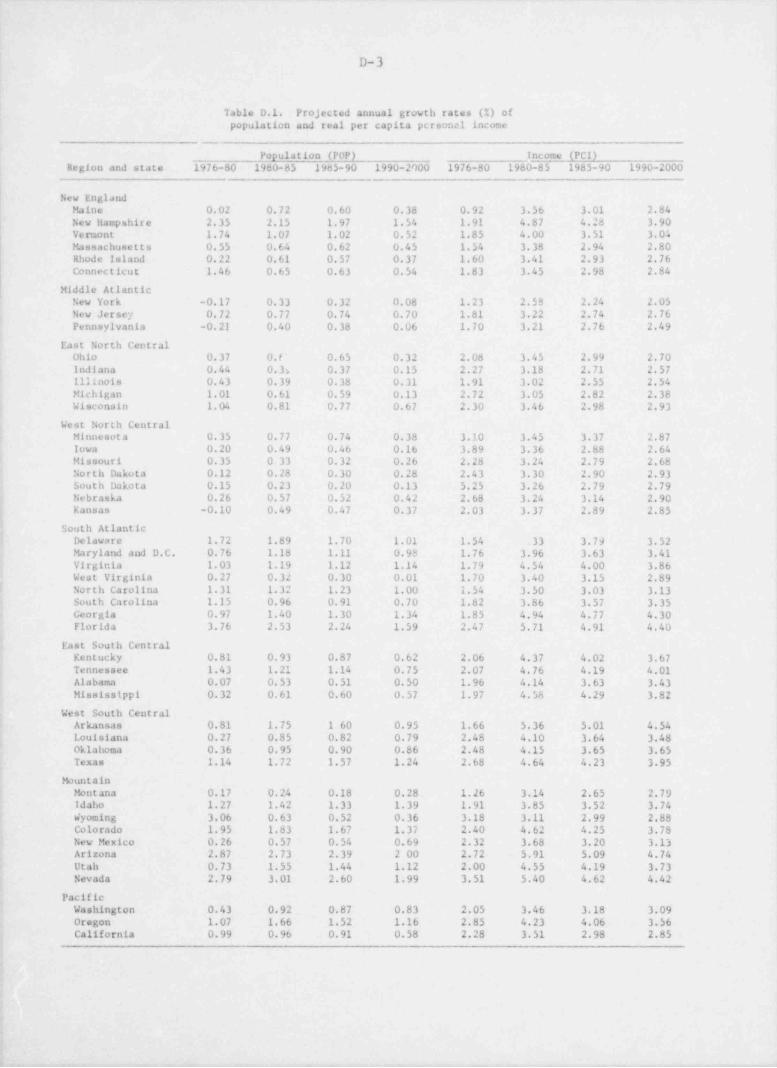
._ . . . _ _ _._ _ _ . _ _ _ _ m. _. . _ _ . . -_

D-3

Table D.1. Projected annual growth rates (%) ofpopulation and real per capita personal income

Population (POP) Income (PCI)Region and state 1976-80 1980-85 1985-90 1990-2000 1976-80 1980-85 1985-90 1990-2000

New EnglandMaine 0.02 0.72 0.60 0.38 0.92 3.56 3.01 2.84

; New Hampshire 2.35 2.15 1.97 1.54 1.91 4.87 4.28 3.90'

Vermont 1.74 1.07 1.02 0.52 1.85 4.00 3.51 3.04Massachusetts 0.55 0.64 0.62 0.45 1.54 3.38 2.94 2.80Rhode Island 0.22 0.61 0.57 0.37 1.60 3.41 2.93 2.76Connecticu t 1.46 0.65 0.63 0.54 1.83 3.45 2.98 2.84

,

! Middle AtlanticNew York -0.17 0.33 0.32 0.08 1.23 2.58 2.24 2.05New Jersey 0.72 0.77 0.74 0.70 1.81 3.22 2.74 2.76Pennsylvania -0.21 0.40 0.38 0.06 1.70 3.21 2.76 2.49

East North CentralOhio 0.37 0. F 0.65 0.32 2.08 3.45 2.99 2.70Indiana 0.44 0.3> 0.37 0.15 2.27 3.18 2.71 2.57,

' 1111nois O.43 0.39 0.38 0.31 1.91 3.02 2.55 2.54Michigan 1.01 0.61 0.59 0.13 2.72 3.05 2.82 2.38

j Wisconsin 1. 04 0.81 0.77 0.67 2.30 3.46 2.98 2.93

West North Central! Minnesot a 0.35 0.77 0.74 0.38 3.10 3.45 3.37 2.87 3

lowa 0.20 0.49 0.46 0.16 3.89 3.36 2.88 2.644

i Missouri 0.35 0.33 0.32 0.26 2.28 3.24 2.79 2.68North Dakota 0.12 0.28 0.30 0.28 2.43 3.30 2.90 2.93South Dakota 0.15 0.23 0.20 0.13 5.25 3.26 2.79 2.79

. Nebraska 0.26 0.57 0.52 0.42 2.68 3.24 3.14 2.90Kansas -0.10 0.49 0.47 0.37 2.03 3.37 2.89 2.85

South AtlanticDelaware 1.72 1.89 1.70 1.01 1.54 .33 3.79 3.52Maryland and D.C. 0.76 1.18 1.11 0.98 1.76 3.96 3.63 3.41

| Virginia 1.03 1.19 1.12 1.14 1.79 4.54 4.00 3.862 West Virginia 0.27 0.32 0.30 0.01 1.70 3.40 3.15 2.89i North Carolina 1.31 1.32 1.23 1.00 1.54 3.50 3.03 3.133 South Carolina 1.15 0.96 0.91 0.70 1.82 3.86 3.57 3.35! Georgia 0.97 1.40 1.30 1.34 1.85 4.94 4.77 4.30

Florida 3.76 2.53 2.24 1.59 2.47 5.71 4.91 4.40: East South Central

Kentucky. 0.81 0.93 0.87 0.62 2.06 4.37 4.02 3.67Tennessee 1.43 1.21 1.14 0.75 2.07 4.76 4.19 4.01Alabama 0.07 0.53 0.51 0.50 1.96 4.14 3.63 3.43Mississippi 0.32 0.61 0.60 0.57 1.97 4.58 4.29 3.82

West South CentralArkansas 0.81 1.75 1 60 0.95 1.66 5.36 5.01 4.54Louisiana 0.27 0.85 0.82 0.79 2.48 4.10 3.64 3.48oklahoma 0.36 0.95 0.90 0.86 2.48 4.15 3.65 3.65Texas 1.14 1.72 1.57 1.24 2.68 4.64 4.23 3.95

MountainMontana 0.17 0.24 0.18 0.28 1.26 3.14 2.65 2.79Idaho 1.27 1.42 1.33 1.39 1.91 3.85 3.52 3.74Wyoming 3.06 0.63 0.52 0.36 3.18 3.11 2.99 2.88Colorado 1.95 1.83 1.67 1.37 2.40 4.62 4.25 3.78New Mexico 0.26 0.57 0.54 0.69 2.32 3.68 3.20 3.13Arizona 2.87 2.73 2.39 2 00 2.72 5.91 5.09 4.74Utah 0.73 1.55 1.44 1.12 2.00 4.55 4.19 3.73Nevada 2.79 3.01 2.60 1.99 3.51 5.40 4.62 4.42

PacificWashington 0.43 0.92 0.87 0.83 2.05 3.46 3.18 3.09Oregon 1.07 1.66 1.52 1.16 2.85 4.23 4.06 3.56California 0.99 0.96 0.91 0.58 2.28 3.51 2.98 2.85

|

||

|

I

liI

_ _ _ _ . . _ _ _ .._. _ _

- - - . - . _. -

D-4

Il1

Table D.2. Projected annual growth rates (%) of the value added in manufacturing

Value added (VA/ WPM)Region and state 1976-b0 19d0-85 1985-90 1990-7000

New EnglandMaine 2.07 3.91 3.33 3.16New Hampshire 2.87 5.10 4.77 4.63Ve rmont 2.82 4.78 4.56 4.57Massachusetts 2.17 4.01 3.74 3.72Rhode Island 2.50 4.50 4.03 4.20Connecticut 2.49 4.23 3.89 3.91

Middle AtlanticNew York 1.74 3.25 2.97 3.21New Jersey 2.62 4.50 4.21 4.22Pennsylvania 2.19 3.69 3.31 3.88

L

East North CentralOhio 2.60 4.36 4.04 4.10Indiana 2.57 ?.54 4.26 4.35Illinois 2.55 4.26 3.94 3.89Michigan 2.34 3.96 3.43 3.56Wisconsin 2.51 4.37 3 95 3.90

West North CentralMinnesota 2.73 4.75 4.36 4.25Iowa 2.95 5 06 4.73 4.69Hissouri 2.49 4.36 3.89 3.95North Dakota 4.62 5.68 5.36 4.77South Dakota 2.85 4.87 4.31 4.55Nebraska 2.89 5.05 4.63 4.32Kansas 3.07 4.69 4.38 4.35

South AtlanticDelaware 3.17 5.29 4.75 4.79Maryland and D.C. 2.27 3.90 3.52 3.59Virginia 2.96 5.11 4.74 4.66West Virginia 2.34 4.10 3.76 3.77North Carolina 3.30 5.53 5.04 4.79South Carolina 3.27 5.93 5.34 5.26Georgia 2.96 5.35 4.62 4.58Florida 3.38 5.81 5.36 5.10

East South CentralKentucky 3.37 5.63 5.32 5.07Tennessee 3.63 5.76 5.38 5.24Alabama 3.06 5.46 4.96 4.91Mississippi 3.35 5.53 5.09 4.95

West South CentralArkansas 3.75 6.37 6.17 6.38Louisiana 3.69 6.25 6.00 6.12Oklahoma 3.72 6.29 6.06 5.89Texas 3.28 5.46 5.12 4.95

HountainMontana 2.56 3.60 3.09 3.38Idaho 3.79 5.58 5.08 5.51Wyoming 3.14 5.28 5.54 5.46

I Colorado 2.70 4.82 4.40 4.31I New Mexico 3.00 5.50 5.10 5.11

Arizona 3.65 6.62 6.46 6.11i -Utah 3.26 5.44 5.22 5.20

Nevada 3.21 5.34 5.05 4.39Pacific

Wash'ngton 2.57 4.14 3.46 3.53Oregon 3.10 4.73 4.08 4.19

; _ California 2.64 4.48 4.13 4.17---

|

, . - ._ _ . - - - .

- . , .- - - - . _ . _ . - _. .- . . - __ .-_- .

D-5

Table D.3. Projected annual growth rates (%) of the numbers ofresidential, commercial, and industrial customers j

Residential customers Commercial customers Industrial customers(CR) (CC) (CI)

Region and state 1926-80 1980-85 1985-2000 1976-80 1980-2000 1976-80 1980-2000

New D. glandMaine 2.8' 2.3 2.0 2.65 2.30 2.65 2.65New Hampshire 2.9 2.7 2.3 4.55 3.88 4.55 4.55Vermont 2.6 2.3 1.9 2.79 2.30 2.79 2.79Massachusetts 1.8 1.5 0.9 0.67 0.40 0.67 0.67Rhode Island 1.1 0.9 0.4 1.27 0.56 1.47 1.47Connecticut 1.9 1.7 1.2 1.04 0.71 1.60 1.60

.,

'

Middle Atlantici New York 1.5 1.5 0.9 1.00 0.60 1.00 1.00! New Jersey 1.5 1.4 1.0 1.39 0.99 1.39 1.39

Pennsylvania 1.4 1.2 0.8 0.94 0.63 0.83 0.83'East North Central

Ohio 1.8 1.5 1.1 1.30 0.95 1.30 1.30Indiana 1.8 1.4 1.1 1.79 1.41 2.21 2.21Illinois 1.8 1.6 1.2 0.86 0.65 1.01 1.01Michigan 2.0 1.8 1.4 1.64 1.28 0.69 0.69Wisconsin 2.2 1.9 1.6 1.26 1.06 0.47 0.47

West North CentralMinremota 2.2 1.9 1.6 1.10 0.93 4.07 4.07Iowa 1.3 1.1 0.8 1.26 0.92 3.60 3.60Missouri 1.7 1.5 1.2 2.35 1.88 5.03 5.08North Dakota 1.4 0.9 0.8 1.23 1.09 3.97 3.97South Dakota 1.2 0.7 0.7 1.14 1.14 2.38 2.38Nebraska 1.9 1.6 1.4 2.42 2.12 2.37 2.37Kansas 1.0 0.9 1.0 1.58 1.76 1.79 1.79

South AtlanticDelaware 2.7 2.3 1.8 2.33 1.82 2.33 2.33thryland and D.C. 1.64 1.66 1.12 1.35 0.91 1.16 1.16Virginia 2.3 1.9 1.5 2.71 2.13 U.95 0.95West Virginia 2.0 1.6 1.4 1.08 0.95 0.96 0.96North Carolir.a 2.65 2.05 1.70 3.36 2.85 1.27 1.27South Carolina 2.67 2.02 1.75 1.79 1.52 1.27 1.27Georgia 2.4 2.0 1.6 3.00 2.45 3.89 3.89Florida 3.9 3.9 3.7 4.53 4.29 5.21 5.21

East South CentralKentucky 2.1 1.7 1.4 2.11 1.74 2.09 2.09Tennessee 2.0 1.7 1.5 2.93 2.59 4.89 4.89Alabama 2.1 1.6 1.3 3.99 3.24 3.86 3.86Hisuissippi 2.5 1.9 1.7 4.02 3.60 2.43 2.43

West South CentralArkansas 2.5 2.1 1.9 '.29 2.07 1.59 1.59Louisiana 2.3 2.0 1.6 1.79 1.43 3.45 3.45Oklahoma 2.1 1.8 1.6 2.22 1.97 1.68 1.68Texas 2.6 2.3 2.1 2.94 2.68 5.58 5.58

MountainMontana 2.2 1.8 1.6 2.63 2.34 2.63 2.63Idaho 2.9 2.5 2.5 3.07 3.07 3.66 3.66Wyoming 2.6 2.0 2.0 3.19 3.19 3.19 3.19Colorado 2.8 2.5 2.2 2.80 3.37 3.00 3.83New Mexico 3.0 2.4 2.2 3.00 3.19 3.42 3.42Arizona 4.2 3.9 3.7 3.80 4.5% 3.27 4.27Utah 2.8 2.5 2.6 2.73 2.84 4.83 5.83Nevada 4.2 4.3 3.7 4.07 4.50 5.63 6.63 ;

'PacificWashington 1.9 1.9 1.5 1,48 1.17 0.85 .0.85Oregon 2.2- 2.1 1.8 3.62 3.13 3.62 3.62California 2.1 2.1 1.7 1.96 1.59 2.48 2.48

:

. _ _ _ _ _ _ _ _ _ _ _ _ _ _ _ _ _ _ _ - _ _ - _ _ _ _ _ - _ _ _ _ _ _ . _ _ _ _ _ _ _ _ _ _ _ _ _ - _ _ _ _ _ _ _ _ _ _ _ _ _ _ _ - _ _ _ _ _ _ _ _ _ _ _ _ _ _ _ _ _ _ _ _ _ - _ _ _ _ - - - - - _ _ _ _ _ _ - _ _ _ ._ _ - _ - -___ _ _ _ _ _ _ _ _ _ _ - _ _ _ _ _ - - - _ _ _ _ _ _ _ _

I

Table D.4. Projected annual growth rates (%) of numbers of natural gas custcmers

Residential customery Commercial customers Industrial customers(RGC) (CGC) (IGC)

Region 1976-80 1980-85 1985-2000 1976-80 1980-85 1985-2000 1976-80 1980-85 1985-2000

New England 0.12 0.04 0.04 0.43 0.17 0.17 -1.16 -1.49 -1.61

Middle Atlantic 0.23 0.19 0.19 0.49 0.40 0.39 -0.86 -0.54 -1.71 7East North Central 1.08 1.04 1.04 1.57 1.46 1.45 -1.00 -0.40 -0.80 *

West North Central 1.14 1.18 1.17 1.53 1.53 1.47 -0.76 -0.98 -1.03

aouth Atlantic 1.44 1.35 1.33 1.27 1.25 1.23 -0.57 -0.70 -1.49

East South Central 1.23 1.27 1.25 0.96 1.00 1.04 -0.91 0 -2.38West South Central 1.03 1.05 1.05 0.84 0.83 0.84 -1.73 -0.55 -1.15

Mountain 2.53 2.41 2.26 2.60 2.08 1.95 0 0 -1.49Pacific 1.06 1.14 1.13 1.20 1.27 1.26 0 -1.3 0

-.

- _ .. . - .. -. _~-----

!

D-7

Table D.5.a. Projected annual growth rates (%) of natural gas (residentialand commercial) price in real terms for the base price case

|Prica of natural gas (PCR) Price of natural gas (PCC) !

Region and state 1976-80 1980-85 1985-90 1990-2000 1976-80 1980-85 1985-90 1990-2000

New EnglandMaine 1.62 1.62 1.12 2.45 1.64 1.64 1.31 2.81

| New Hampshire 1.62 1.62 1.12 2.45 1.64 1.64 1.31 2.81* Vermont 1.62 1.62 1.12 2.45 1.64 1.64 1.31 2.81

Massachusetts 1.62 1.62 1.12 2.45 1.64 1.64 1.31 2.81Rhode Island 1.62 1.62 1.12 2.45 1.64 1.65 1.31 2.81Connecticut 1.62 1.62 1.12 2.45 1.64 1.64 1.31 2.81

Middle AtlanticNew York 2.73 2.73 2.44 2.59 2.34 2.34 2.83 2.91New Jersey 2.73 2.73 2.44 2.59 2.34 2.34 2.83 2.91Pennsylvania 3.84 3.84 1.71 1.39 2.88 2.88 1.90 1.60

East North CentralOhio 5.04 5.04 1.28 3.15 4.95 4.95 1.42 3.51Indiana 5.04 5.04 1.28 3.15 4.95 4.95 1.42 3.511111nois 5.04 5.04 1.28 3.15 4.95 4.95 1.42 3.51Michigan 5.04 5.04 1.28 3.15 4.95 4.95 1.42 3.51Wisconsin 5.04 5.04 1.28 3.15 4.95 4.95 1.42 3.51

West North Central,

; Minnesota 5.04 5.04 1.28 3.15 4.95 4.95 1.42 3.51- Iowa 5.95 5.95 2.33 1.94 6.95 5.95 2.66 2.121 Missouri 5.95 5.95 2.33 1.94 6.95 6.95 2.66 2.12! horth Dakota 9.14 9.14 1.34 3.18 10.13 10.13 1.44 3.38{ South Dakota 9.14 9.14 1.34 3.18 10.13 10.13 1.44 3.38

Nebraska 5.95 5.95 2.33 1.94 6.95 6.95 2.66 2.12Kansas 5.95 5.95 2.33 1.94 6.95 6.95 2.66 ?.12

South Atlantic.

Delaware 3.84 3.84 1.71 1.39 2.88 2.88 1.90 1.60Maryland and D.C. 3.84 3.84 1.71 1.39 2.88 2.88 1.90 1.60

i Virginia 3.84 3.84 1.71 1.39 2.88 2.88 1.90 1.60West Virginia 3.84 3.84 1.71 1.39 2.88 2.88 1.90 1.60North Carolina 4.54 4.54 1.50 1.39 3.98 3.98 1.77 1.63South Carolina 4.54 4.54 1.50 1.39 3.98 3.98 1.77 1.63

; Georgia 4.54 4.54 1.50 1.39 3.98 3.98 1.77 1.63 '~

Florida 4.54 4.54 1.50 1.39 3.98 3.98 1.77 '.63 i

iEast South CentralKentucky 4.54 4.54 1.50 1.39 3.98 '3.98 1.77 1.63Tennessee 4.54 4.54 1.50 1.39 3.98 3.98 1.77 1.63Alabama 4.54 4.54 1.50 1.39 3.98 3.98 1.77 1.63Mississippi 4.54 4.54 1.50 1.39 3.98 3.98 1.77 1.63

West South Central. Arkansas 5.86 5.86 1.50 3.00 7.57 7.57 1.83 3.47I Louisiana 5.86 5.86 1.50 3.00 7.57 7.57 1.83 3.47! Oklahoma 5.86 5.86 1.50 3.00 7.57 7.57 1.83 3.47i Texas 5.86 5.86 1.50 3.00 7.57 7.57 1.83 3.47' Mountaini Montana 9.14 9.14 1.34 3.18 10.13 10.13 1.44 3.38' Idaho 6.05 6.05 2.35 -0.04 b.19 6.19 2.68 -0.04

Wyoming 9.14 9.14 1.34 3.18 10.13 10.13 1.44 3.38Colorado 9.14 9.14 1.34 3.18 10.13 10.13 1.44 3.38

. New Mexico 5.86 5.86 1.50 3.00 4.57 4.57 1.83, 3.47i Arizona 8.96 8.96 0.55 0.58 6.42 6.42 0.63 0.67

Utah . 9.14 9.14 1.34 3.18 10.13 10.13 1.44 3.38Nevada 8.96 8.96 0.55 0.58 6.42 6.42 0.63 0.67,

'

PacificWashington 6.05 6.05 2.35 -0.04 6.19 6.19 2.68 -0.04Oregen . 6.05 6.05 2.35 -0.04 6.19 6.19 2.68 -0.04California 8.96 8.96' O.55 0.58 6.42 6.42 0.63 0.67

L4

9

__ - _ _ , _ . , _ , - . _ , _ . _ _ , _ - - _ -

D-8

Table D.5.b. Projected annual growth rates (2) of natural gas (PCI)and coal price in real terma for the base price case

Price of natural gas (PC1) Price of coal (PCl,Region and state 1976-80 1980-85 198)-90 1990-2000 1976-80 1960-85 1985-90- 1990-2000

New EnglandMaine 4.55 4.55 2.05 5.85 -1.36 -1.36 1.49 1.14New nampshire 4.55 4.55 2.05 5.85 -1.36 -1.36 1.49 1.1/.Vermont 4.55 4.55 2.05 5.85 -1.36 -1.36 1.49 1.14Massachusetts 4.55 4.55 2.05 5.85 -1.36 -1.36 1.49 1.14Rhode Island 4.55 4.55 2.05 5.85 -1.36 -1.36 1.49 1.14Connecticut 4.55 4.55 2.05 5.85 -1.36 -1.36 1.49 1.14


East North CentralOhio 7.54 7.54 5.16 7.60 1.22 1.22 1.28 1.21Indiana 7.54 7.54 5.16 7.60 1.22 1.22 1.28 1.21Illinois 7.54 7.54 5.16 7.60 1.22 1.22 1.28 1.21Michigan 7.54 7.54 5.16 7.60 1.22 1.22 1.28 1.21Wisconsin 7.54 7.54 5.16 7.60 1.22 1.22 1.28 1.21

|

West North CentralMinncsota 7.54 7.54 5.16 7.60 1.22 1.22 1.28 1.21lowa 10.63 10.63 4.81 6.98 1.67 1.67 1.11 1.17Missouri 10.63 10.63 4.81 6.98 1.67 1.67 1.11 1.17North Dakota 11.65 11.65 1.75 3.82 0.28 0.28 0.17 1.81South Dakota 11.65 11.65 1.75 3.82 0.28 0.28 0.17 1.81Nebraska 10.63 10.63 4.81 6.98 1.67 1.67 1.11 1.17Kansas 10.63 10.63 4.81 6.98 1.67 1.67 1.11 1.17

South AtlanticDelaware 5.97 5.97 3.79 5.02 2.91 2.91 1.81 1.18Maryland and D.C. 5.97 5.97 3.79 5.02 2.91 2.91 1.81 1.18Virginia 5.97 5.97 3.79 5.02 2.91 2.91 1.81 1.18West Virginia 5.97 5.97 3.79 5.02 2.91 2.91 1.81 1.18North Carolina 9.15 9.15 3.66 5.76 3.48 3.48 1.33 1.06South Carolina 9.15 9.15 3.66 5.76 3.48 3.48 1.33 1.06Georgia 9.15 9.15 3.66 5.76 3.48 3.48 1.33 1.06Florida 9.15 9.15 3.66 5.76 3.48 3.48 1.33 1.06

East South CentralKentucky 9.15 9.15 3.66 5.76 3.48 3.48 1.33 1.06Tennessee 9.15 9.15 3.06 5.76 3.48 3.48 1.33 1.06Alabama 9.15 9.15 3.66 5.76 3.48 3.48 1.33 1.06Mississippi 9.15 9.15 3.66 5.76 3.48 3.45 1.33 1.06

West South CentralArkansas 11.24 11.24 2.03 3.80 0.59 0.59 1.02 1.08Louisiana 11.24 11.24 2.03 3.80 0.59 0.59 1.02 1.08Oklahoma 11.24 11.24 2.03 3.80 0.59 0.59 1.02 1.08Texas 11.24 11.24 2.03 3.80 0.59 0.59 1.02 1.08

HountainMontana 11.65 11.65 1.75 3.82 0.28 0.28 0.17 1.81idaho 9.73 9.73 1.16 6.47 1.92 1.92 0.21 1.14Wyoming 11.65 11.65 1.75 3.82 0.28 0.28 0.17 1.81Colorado 11.65 11.65 1.75 3.82 0.28 0.28 0.17 1.81New Mexico 11.24 11.24 2.03 3.80 0.59 0.59 1.02 1.08Arizona 8.96 8.96 2. 04 3.48 4.99 4.99 1.46 1.35Utah 11.65 11.65 1.75 3.82- 0.28 0.28 0.17 1.81Nevada 8.96 8.96 2.04 3.48 4.99 4.99 1.46 1.35


:

!

4

- - ,

. ~ , , .- . -- . _ . - - . .. -- -

I

D-9

|!

Table D.5.c. Projected annual growth rates (%) of oil pricesin real terms for the base price case

Price of No. 2 oil (POR) Price of No. 6 oil (P01)

Region and state 1976-80 1980-85 1985-90 1990-2000 1976-80 1980-85 1985-90 1990-2000

| New England i

j Maine 4.07 4.07 1.70 5.03 5.23 2.23 1.46 5.43 ,

New Hampshire 4.07 4.07 1.70 5.03 5.23 5.23 1.46 5.41 i'

Vermont 4.07 4.07 1.70 5.03 5.23 5.23 1.46 5.43Massachusetts 4.07 4.07 1.70 5.03 5.23 5.23 1.46 5.43

; Rhode Island 4.07 4.07 1.70 5.03 5.23 5.23 1.46 5.43Connecticut 4.07 4.07 1.70 5.03 5.23 5.23 1.40 5.43


East North CentralOhio 4.36 4.36 1.90 5.31 4.00 4.00 1.63 5.694

4 Indiana 4.36 4.36 1.90 5.31 4.00 4.00 1.63 5.69111tnois 4.36 4.36 1.90 5.31 4.00 4.00 1.63 5.69Michigan 4.36 4.36 1.90 5.31 4.00 4.00 1.63 5.69i

Wisconsin 4.36 4.36 1.90 5,31 4.00 4.00 1.63 5.69

West North CentralMinnesota 4.36 4.36 1.90 5.31 4.00 4.00 1.63 5.69

4

lowa 4.44 4.44 1.92 5.37 6.03 6.03 1.62 5.61Missouri 4.44 4.44 1.92 5.37 6.03 6.03 1.62 5.61North Dakota 4.75 4.75 1.88 5.27 5.77 5.77 1.70 5.80South Dakota 4.75 4.75 1.88 5.27 5.77 5.77 1.70 5.80

i Nebraska 4.44 4.44 1.92 5.37 6.03 6.03 1.62 5.61Kansas 4.44 4.44 1.92 5.37 6.03 6.03 1.62 5.61

South AtlanticDelaware 5.08 5.08 1.69 4.87 6.70 6.70 1.37 5.18

; Maryland and D.C. 5.08 5.08 1.69 4.87 6.70 6.70 1.37 5.18'

Virginia 5.08 5.08 1.69 4.87 6.70 6.70 1.37 5.18i West Virginia 5.08 5.08 1.69 4.87 6.70 6.70 1.37 5.18i North Carolina 5.69 5.69 1.67 4.87 6.28 6.28 1.65 5.65

South Carolina 5.69 5.69 1.67 4.87 6.28 6.28 1.65 5.65Georgia 5.69 5.69 1.67 4.87 6.28 6.28 1.65 5.65Florida 5.69 5.69 1.67 4.87 6.28 6.28 1.65 5.65

East South Centralj Kentucky 5.69 5.69 1.67 4.87 6.28 6.28 1.65 5.65

Tennessee 5.69 5.69 1.67 4.87 6.28 6.28 1.65 5.65Alabama 5.69 5.69 1.67 4.87 6.28 6.28 1.65 5.65Mississippt 5.69 5.69 1.67 4.87 6.28 6.28 1.65 5.65

West South Centralj Arkansas 6.00 6.00 1.82 5.11 7.48 7.48 1.63 5.64

Louisiana 6.00 6.00 1.82 5.11 7.48 7.48 1.63 5.64Oklahoma 6.00 6.00 1.82 5.11 7.48 7.48 1.63 5.64' taxa s 6.00 6.00 1.82 5.11 7.48 7.48 1.63 5.64

i

h.untain, Montana 4.75 4.75 1.88 5.27 5.77 5.77 1.70 5.80

Idaho 4.58 4.58 0.50 5.44 5.02 5.02 -0.05 6.01*

i Wyoming 4.75 4.75 1.88 5.27 5.77 5.77 1.70 5.80-Colorado 4.75 4.75 1.88 5.27 5.77 5.77 1.70 5.80

New Mexico 6.00 6.00 1,82 5.11 7.48 7.48 1.63 5.64Arizona 4.44 4.44 0.50 5.44 4.70 4.70 -0.05 6.09Utah 4.75 4.75 1.88 5.27 5.77 5.77 1.70 5.80 |

Nevada 4.44 4.4l 0.50 5.44 4.70 4.70 -0.05 6.01'

PacificWashington 4.58 4.58 0.50 5.44 5.02 5.02 -0.05 6.01 j

Oregon 4.58 4.58 0.50 5.44 5.02 5.02 -0.05 6.01 ;

California 4.44 4.44 0.50 5.44 4.70 4.70 -0.05 6.09

2

4

- - , - , , . - n,-- w - y,m - - ,,,,w. -----v-- ---

.. _ _ . - ._ _ .-

<

D-10

Table D.6.a. Projected annual growth rates (%) of natural gas (residentialand commercial) price in real terms for the high price case

Price of natural gas (PCR) Price of natural gas (PCC)Region and state 1976-80 1980-85 1985-90 1990 2000 1976-80 1980-85 1985-90 1990-2000

New EnglandMaine 3.24 3.24 2.24 4.90 3.28 3.28 2.62 5.62New Hampshire 3.24 3.24 2.24 4.90 3.28 3.28 2.62 5.62Vermont 3.24 3.24 2.24 4.90 3.28 3.28 2.62 5.62Massachusetts 3.24 3.24 2.24 4.90 3.28 3.28 2.62 5.62Rhode Island 3.24 3.24 2.24 4.90 3.28 3.28 2.62 5.62Connecticut 3.24 3.24 2.24 4.90 3.28 3.28 2.62 5.62

Middle AtlanticNew York- 5.46 5.46 4.88 5.18 4.68 4.68 5.66 5.82;

| New Jersey 5.46 5.i6 4.88 5.18 4.68 4.68 5.66 5.82Pennsylvania 7.68 7.68 3.42 2.78 5.76 5.76 3.80 3.20

East North CentralOhio 10.08 10.08 2.56 6.30 9.90 9.90 2.84 7.024

Indiana 10.08 1 0. 08 2.56 6.30 9.90 9.90 2.84 7.02Illinois 10.08 10.08 2.56 L.30 9.90 9.90 2.84 7.02Michigan 10.08 10.08 2.56 6.30 9.90 9.90 2.84 7.02i

Wisconsin 10.08 10.08 2.56 6.30 9.90 9.90 2.84 7.02 ;

, West North Centralj Minnesota 10.08 10.08 2.56 6.30 9.90 9.90 2.b4 7.02

Iowa 11.90 11.90 4.66 3.88 13.90 13.90 5.32 4.24Missouri 11.90 11.90 4.66 3.88 13.90 13.90 5.32 4.24North Dakota 18.28 18.28 2.68 6.36 20.26 20.26 2.88 6.76South Dakota 18.28 18.28 2.68 6.36 20.26 20.26 2.88 6.76Nebraska 11.90 11.90 4.66 3.88 13.90 13.90 5.32 4.24Kansas 11.90 11.90 4.66 3.88 13.90 13.90 5.32 4.24

South AtlanticDelaware 7.68 7.68 3.42 2.78 5.76 5.76 3.80 3.20Maryland and D.C. 7.68 7.66 3.42 2.78 5.76 5.76 3.80 3.20Virginia 7.68 7.68 3.42 2.78 5.76 5.76 3.80 3.20West Virginia 7.68 7.68 3.42 2.78 5.76 5.76 3.80 3.20North Carolina 9.08 9.08 3.00 2.78 7.96 7.96 3.54 3.26South Carolina 9.08 9.08 3.00 2.78 7.96 7.96 3.54 3.26Georgia 9.08 9.08 3.00 2.78 's.96 7.96 3.54 3.26Florida 9.08 9.08 3.00 2.78 7.96 7.96 3.54 3.26

East South CentralKentucky 9.08 9.08 3.00 2.78 7.96 7.96 3.54 3.26

'

Tennessee 9.08 9.08 3.00 2.78 7.96 7.96 3.54 3.26Alab ama 9.08 9.08 3.00 2.78 7.96 7.96 3.54 3.26Mississippi 9.08 9.08 3.00 2.78 7.96 7.96 3.54 3.26

West South CentralArkansas 11.72 11.72 3.00 6.00 15.14 15.14 3.66 6.94Louisiana 11.72 11.72 3.00 6.00 15.14 15.14 3.66 6.94oklahoma 11.72 11.72 3.00 6.00 15.12 15.14 3.66 6.94Texas 11.72 11.72 3.00 6.00 15.14 15.14 3.66 6.94

HountainMontana 18.28 18.28 2.68 6.36 20.26 20.26 2.88 6.76Idaho 12.10 12.10 4.70 -0.02 12.38 12.38 5.36 - 0.02Wyoming 18.28 -18.28 2.68 6.36 20.26 20.26 2.88 6.76colorado 18.28 18.28 2.68 6.36 20.26 20.26 2.88 6.76New Mexico. 11.72 11.72 3.00 6.00 15.14 15.14 3.66 6.94Arizona 17.92 17.92 1.10 1.16 12.84 12.84 1.26 1.34Utah 18.28 18.28 2.68 6.36 20.26 20.26 2.88 6.76Nevada 17.92 17.92 1.10 1.16 12.84 12.84 1.26 1.34

PacificWashington 12.10 12.10 4.70 - 0.02 12.38 12.38 5.36 - 0.02Oregon 12.10 12.10 4.70 - 0.02 12.38 12.38 5.36 - 0.02California 17.92 17.92- 1.10 1.16 12.84 12.84 1.26 1.34

_

T

_ . -,

I

ii|

l|

D-11

Table D.6.b. Projected annual growth rates (%) of natural gas (industrial)and coal prices in real terms for the high price case

Price of natural gas (PCI) Price of ceal (PC)Region and state 1976-80 1980-85 1985-90 1990-2000 1976-80 1980-85 1985-90 1990-2000

New EnglandHaine 9.10 9.10 4.10 11.70 -0.68 -0.68 2.98 2.28New Hampshire 9.10 9.10 4.10 11.7C -0.68 -0.68 2.98 2.28Vermont 9.10 9.10 4.10 11.70 -0.68 -0.68 2.98 2.28Hassac huse t t s 9.10 9.10 4.10 11.70 -0.08 -0.68 2.98 2.28Rhode Island 9.10 9.10 4.10 11.70 -0.68 -0.68 2.98 2.28Connecticut 9.10 9.10 4.10 11.70 -0.68 -0.68 2.98 2.28

Middle AtlanticNew iork 16.50 16.50 4.32 8.26 3.68 3.68 3.38 2.22New Jersey 16.50 16.50 4.32 8.26 3.68 3.68 3.38 2.22Pennsylvania 11.94 11.94 7.58 10.04 5.82 5.82 2.66 2.12

East North CentralOhio 15.08 15.08 10.32 15.20 2.44 2.44 2.56 2.42Indiana 15.08 15.08 10.32 15.20 2.44 2.44 2.56 2.42Illinois 15.08 15.08 10.32 15.20 2.44 2.44 2.56 2.42Michigan 15.08 15.08 10.32 15.20 2.44 2.44 2.56 2.42Wisconsin 15.08 15.08 10.32 15.20 2.44 2.44 2.56 2.42

West North CentralHinnesota 15.08 15.08 10.32 15.20 2.44 2.44 2.56 2.42lowa 21.26 21.26 9.62 13.96 3.34 3.34 2.22 2.34Missouri 21.26 21.26 9.62 13.96 3.34 3.34 2.22 2.34North Dakota 23.30 23.30 3.50 7.64 0.56 0.56 0.34 3.62South Dakota 23.30 23.30 3.50 7.64 0.56 0.56 0.34 3.62Nebraska 21.26 21.26 9.62 13.96 3.34 3.34 2.22 2.34Kansas 21.26 21.26 9.62 13.96 3.34 3.34 2.22 2.34

South AtlanticDelaware 11.94 11.94 7.5E 10.04 5.82 5.82 3.62 2.36Furyland and D.C. 11.94 11.94 7.38 10.04 5.82 5.82 3.62 2.36Virginia 11.94 11.94 7.58 10.04 5.82 5.82 3.62 2.36West Virginia 11.94 11.93 7.58 10.04 5.82 3.82 3.62 2.36North Carolina 18.30 18.30 7.32 11.52 6.96 6.96 2.66 2.12South Carolina 18.30 18.30 7.32 11.52 6.96 6.96 2.66 2.12Georgia 18.30 18.30 7.32 11.52 6.96 6.06 2.66 2.12Florida 18.30 18.30 7.32 11.52 6.96 6.96 2.66 2.12

East South CentralKentucky 18.10 '8.30 7.32 11.52 c.96 6.96 2.66 2.12Tennessee 18.3u 18.30 7.32 11.52 6.96 6.96 2.66 2.12Alabama 18.30 18.30 7.32 11.52 6.96 6.96 2.66 2.12

4

Mississippi 18.30 18.30 7.32 11.52 6.96 6.96 2.66 2.12West South Central

Arkansas 22.48 22.48 4.06 7.60 1.18 1.18 2.04 2.08Louisiana 22.48 22.48 4 nt 7.60 1.18 1.18 2.04 2.08Oklahosa 22.48 22.48 4.06 7.6s 1.18 1.18 2.04 2.08Texas 22.48 22.48 4.06 7.60 1.18 1.18 2. 04 2,08

HountainMontana 23.30 23.30 3.50 7.64 0.56 0.56 0.34 3.62Idaho 19.46 19.46 2.32 12.94 3.84 3.84 0.42 2.26Wyoming 23.30 23.30 3.50 7.64 0.56 0.56 0.34 3.62Colorado 23.30 23.30 3.50 7.64 0.56 0.56 0.34 3.62New Mexico 22.48 22.48 4.06 7.60 1.18 1.18 2.04 2.16Arizona 17.92 17.92 4.08 6.96 9.98 9.98 2.92 2.70Utah 23.30 23.30 3.50 7.64 0.56 0.56 0.34 3.62Nevada 17.92 17.92 4.08 6.96 9.98 9.98 2.92 2.70


.

hb

. . . . . - . - -. .. _ _ . = . . - - . . _ . _ _ .

1 D-12

I4ble D.6.c. Projected annual growth rates (%) of oil pricesin real terms for the high price case

t

Price of.No. 2 oil (POR) Price of No. 6 oil (POI)4

Region and state 1976-80 1980-85 1985-90 1990-2000 1976-80 1980-85 1985-90 1990-2000

Ij New England

Maine 8.14 8.14 3.40 10.06 10.46 10.46 2.92 10.86New Hampshire 8.14 8.14 3.40 10.06 10.46 10.46 2.92 10.86'

Vermont 8.14 8.14 3.40 10.06 10.46 10.46 2.92 10.86; Massachusetts 8.14 8.14 3.40 10.06 10.46 10.46 2.92 10.86

Rhode Island 8.14 8.14 3.40 10.06 10.46 10.46 2.92 10.86Connecticut 8.14 8.14 3.40 10.06 10.46 10.46 2.92 10.96

'

Middle AtlanticNew York 9.06 9.06 3.50 9.98 12.24 1. . v4 2.82 10.62New Jersey 9.06 9.06 3.50 9.98 12.24 12.74 2.82 10.62Pennsylvan'a 10.16 10.16 3.38 9.74 13.40 13 40 2.74 10.36

East North CentralOhio 8.72 8.72 3.80 10.62 8.00 8.00 3.26 11.38Indiana 8.72 8.72 3.80 10.62 8.00 8.00 3.26 11.38

- Illinois 8.72 8.72 3.80 10.62 8.00 8.00 3.26 11.38Michigan 8.72 8.72 3.80 10.62 8.00 8.00 3.26 11.38'

Wisconsin 8.72 8.72 3.80 10.62 8.00 8.00 3.26 11.38

f' Minnesota 8.72 8.72 3.80 10.62 8.00 8.00 3.26 11.38West North Central

Iowa 8.88 8.88 3 84 10.74 12.06 12.06 3.24 11.22Missouri 8.88 8.88 3.84 10.74 12.06 12.06 3.24 11.22North Dakota 9.50 9.50 . 76 10.54 11.54 11.54 3.40 11.60

) South Dakota 9.50 9.50 3.76 10.54 11.54 11.54 3.40 11.60' Nebraska 8.88 P.88 3.84 10.74 12.06 12.06 3.24 11.22

i Kansac 8.88 8.88 3.84 10.74 12.06 12.06 3.24 11.22

South AtlanticDelaware 10.16 10.16 3.38 9.74 13.40 13.40 2.74 10.36Maryland and D.C. 10.16 10.16 3.38 9.74 13.40 13.40 2.74 10.36Virginia 10.16 10.16 3.38 9.74 13.40 13.40 2.74 10.36West Virginia 10.16 10.16 3.38 9.74 13.40 13.40 2.74 10.36North Carolina 11.38 11.38 3.34 9.74 12.56 12.56 3.30 11.30

#'South Carolina 11.38 11.38 3.34 9.74 12.56 12.56 3.30 11.30ceorgia 11.38 11.38 3.34 9.74 12.56 12.56 3.30 11.30Florida 11.38 11.38 3.34 9.74 12.56 12.56 3.30 11.30

,

' East South CentralKentucky 11.38 11.38 3.34 9.74 12.56 12.56 3.30 11.30'

4 Tennessee 11.38 11.38 3.34 9.74 12.56 12.56 3.30 11.30Alabama 11.38 11.38 3.34 9.74 12.56 12.56 3.30 11.30Mississippi 11.33 11.38 3.34 9.74 12.56 12.5b 3.40 - 11.30

West touth CentralArkansas 12.00 12.00 3.64 10.22 14.96 14.96 3.26 11.28Louisiana 12.00 12.00 3.64 10.22 14.96 14.96 3.26 11.28Oklahoma 12.00 12.00 3.64 10.22 14.96 14.96 3.26 11.28Texas 12.00 1z.00 3.64 10.22 14.96 14.96 3.26 11.28

HountainMontana 9.50 9.50 3.76 10.54 11.54 11.54 3.40 11.60Idaho 9.16 9.16 1.00 10.88 10.04 10.04 -0.03 12.02Wyoming 9.50 9.50 3.76 10.54 11.54 11.54 3.40 11.60colorado 9.50 9.50 3.76 10.54 11.54 11.54 3.40 11.60New Mexico 12.00' 12.00 3.64 10.22 14.96 14.96 3.26 11.28Arizona 8.88 8.88 1.00 10.88 9.40 9.40 -0.03 12.18Utah 9.50 9.50 3.76 10.54 11.54 11.54 3.40 11.60*

; Nevada 8.88 8.68 1.00 10.88 9.40 9.40 -0.03 12.02

PacificWashington 9.16 9.16 1.00 10.88 10.04 10.04 -0.03 12.02Oregon 9.16 9.16 1.00 10.88 10.04 10.04 -0.03 12.02

,

California 8.88 8.68 1.00- 10.88 9.40 9.40 -0.03 12.18I

.., . -. . . - - -. .

. . -. . ___ .-- . . . ... .. _- - .----

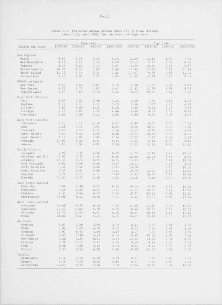
D-13

Table D.7. Projected annual growth rates (%) of total averageelectricity cost (TOC) for the base and high cases

Base case High case

Region and state 1976-80 1980-85 1985-90 1990-2000 1976-80 1980-85 1985-90 1990-2000 [

| New EnglandMaine 9.89 8.76 6.45 6.52 12.69 13.10 8.50 7.91New Hampshire 9.27 ~ 7.20 6.16 6.59 10.13 8.97 7.06 8.62Vermont 9.25 8.24 6.10 5.97 10.54 10.54 7.73 6.67Massachusetts 10,38 9.35 5.93- 7 38 12.96 12.60 7.11 11.19

| Rhode Island 10.72 6.16 6.31 7.81 13.67 9.48 7.68 11.71| Connec ticut 9.95 9.06 6.22 7.05 12.32 12.43 7.86 9.86t

} Middle AtlanticNew York 9.86 8.84 6.03 6.70 11.56 11.32 6.92 9.15

,

New Jersey 9.73 8.79 5.87 6.67 11.91 11.78 6.91 9.58Pennsylvania 9.45 8.40 6.18 6.04 10.73 10.21 7.14 7.21

1 East North CentralOhio 8.07 7.03 6 06 5.15 8.60 7.74 6.83 6.03Indiana 8.12 7.17 6.12 5.23 8.56 7.87 6.73 6.03Illinois 9.03 8.00 6.19 6.18 9.95 9.44 7.36 7.53Michigan 9.18 8.07 6.28 6.46 10.30 9.69 7.55 8.42Wisconsin 9.09 7.99 6.12 5.95 9.99 9.45 7.38 6.93;

f West North Centrali Minnesota 9.10 8.11 6.16 6.07 9.99 9.47 7.30 7.05| Iowa 9.28 8.18 5.97 6.23 10.26 10.27 6.75 7.68

Missouri 8.48 7.49 6.14 5.16 9.15 8.70 6.90 5.754

1 North Dakota 9.40 8.42 6.09 6.38 10.73 10.65 7.35 8.01South Dakota 8.14 7.07 5.98 5.14 8.27 7.32 6.06 5.53Nebraska 10.00 8.58 6.44 6.53 12.25 12.14 8.79 9.19

-I Kansas 9.89 8.98 6.92 7.00 12.52 13.34 9.66 11.81i South Atlantic

Delaware 9.99 9.38 6.36 6.99 12.15 13.18 7.46 10.81Maryland and D.C. 9.94 9.24 5.93 6.45 11.89 12.09 6.96 8.96

*Virginia 10.35 9.18 6.05 6.95 13.35 11 *1 7.41 10.25

- West Virginia 8.82 7.86 6.36 5.17 10.11 1.36 5.93) North Carolina 9.34 8.54 5.86 7.11 10.70 6.73 10.20' South Carolina 9.34 8.54 5.86 7.11 10.70 .9.21 6.73 10.20

Georgia 9.71 8.73 6.17 7.43 11.33 10.97 7.10 10.66<

) Florida 10.63 9.77 6.40 7.84 13.46 '3.58 7.80 12.03

East South CentralKentucky 8.84 7.90 6.12 6.85 10.04 9.40 6.72 10.09Tennessee 9.29 8.25 6.17 7.71 11.07 10.75 7.29 11.25

j Alabama 9.37 8.46 6.13 7.26 10.72 10.26 7.01 10.10Mississippi 10.96 8.42 6.38 7.91 14.42 12.77 8.06 12.24'

) West South Central; Arkansas 10.69 9.78 6.28 7.30 14.18 14.17 7.78 10.96'

Louisiaan 12.67 11.82 6.30 6.89 18.44 19.90 7.76 10.59Oklahoma 12.74 12.14 6.41 o.60 18.61 20.66 8.16 10.15 !

;, Texas 11.81 11.47 6.45 6.56 16.92 19.48 8.10 10.07 I

tbuntainMontana 8.04 7.16 5.96 5.09 8.11 7.30. 6.01 5.33Idaho 6.01 7.02 6.00 5.02 8.03 7.06 6.01 5.09 I,

Wyoming 7.97 6.93 5.89 5.17 8.07 7.06 5.95 5.591 Colorado 2.65 7.99 5.93 5.60 9.90 10.71 6.54 7.51

New Mexico 9.30 8.87 6.24 5.85 11.32 13.08 7.31 8.38Arizona 8.70 7.61 5.92 5.66 9.64 9.15 6.34 7.43Utah 8.36 7.26 5.88 5.35 8.82 8.25 6.16 6.38Nevada 9.25 8.43 6.10 5.48 10.99 11.23 6.86 7.04

PacificWashington 8.14 7.19 6.08 5.09 8.31 7.77 6.63 5.46Otegon -8.18 '7.05 6.18 5.19 8.37 7.40 6.87 5.72

4

California 10.02 9.52 5.68 7.59 13.24 13.86 6.34 11.87!4

4

|

|

|

*-__ _. ~~. , .-_ _ _ . . _ _ _. . _ _ _ . -, , _.

- - - .._- .__ . - ._

!

|

Appendix E

FORECASTS OF ELECTRICITY DEMAND AND PRICE BY STATEAND BY REGION: 1980, 1985, 1990, 1995, AND 2000

J

b

7

I

J

i

i

I

.

"~ - - ,---s .- .. _.- , ,_ ,

. _ _ _ _ _ _ _ _ _ _ _

M* U EMGLAND ROCICN V EPS ION II EAS E CASM

FOPECASTS O' EL ETT37CI~7 DEM A Nt (1001 GIC Ad ATT i!OURS)

17 7 C A CT U A L lon0 1995 1900

STATP PES CCF IND TOTAL RES COM IND TCTAL FIS COM TND TOTAL BYS C05 IND TOTAL

9 AIDE 2. P 1.* 2.3 6.4 3. ' ?.2 2. 5 2.P 5.0 3. 2 3.1 1 1. ' 6.2 4. 4 3.9 15.1

N FF HA9PSHTTC 2. 3 S.C 2.0 5.1 2.8 1. 2 2. 2 6.2 '.A 1. 9 2. 8 1.5 5.0 J.1 3.9 12.1

V'P 5C ET 1. 5 0.t C. 0 3.1 1. 9 0. P 1. 0 1.9 2.4 1. 2 1. 3 5.2 3.1 1.7 1.7 6.9

MASSAC10SFTTS 1 1. . 10. f 7. 9 31.0 12.1 11.6 a. 4 33.1 13.5 13.5 10.3 29.8 15.7 16.3 13.2 46.5

PFCCE ISLAND 1. ') 1.! 1. 3 4.4 1. 9 1.5 1. 4 5.0 2.1 1.8 1.9 5. 0 2.5 2. 2 2.4 7. 3

CCMNICTICUT ~.0 6.C 5.0 19.5 9. 9 6.0 f.4 22.5 10.5 8. 2 0.1 27.1 12.3 9.9 10.4 33.3

S ECIC N AL TOT 1L !.P. 0 21.1 1 C. S 70.R 31.4 24.2 21.9 '9.5 37.3 21.7 2'. 4 96.9 44.9 37.5 35.4 120.R

1915 2301

STATE PES CUP IND TCTAL 355 CDE I4D TCTRL

MMISE 7. 5 5.( 4.8 18.6 9. 9 6.9 5." 22.5m

N9W HA'2SHInt 6. 4 4.' 5.2 16.5 9. 0 6 . f. 7.1 22.0 8.

w

VYPMCNT * R 2.2 2.3 a.R 4. 5 2 ~. e 3.1 11.1

MASSACHts!"TS 1,. 10 . 0 16.7 54.4 19.1 21.5 21.1 6 3. !

SECTE ISLAND 2. 6 ' . ' 3.1 9.5 2. 6 2. ' 4.0 9.'

CC N E E CTICf!T'

11. 4 13.4 39.1 15.4 13.2 17.2 46.4

FECICNtL T0"TL 52. 0 45.* 45.5 146.7 59.6 51.9 58.4 175.1

FO R EC AST ED A NM DA L G. sd ., thTE3 0F ELECTRICITY DEMAND TCR 10'6-1900 ( P EPC INT)

STATE , RSS CCM IND TCTAL

9AT12 5. S 7.8 3. 7 3.'

NIE HA9FSHIRE 5. 7 9.1 4. 9 6.1

VFRMcNT 5. 1 7.9 4. 2 5.4

9ASSAC9CSMTTS 2. 2 3.1 1. 7 2.0 ,-

PfCEE ISLAND 2.1 2.9 4. 2 3. 0

CrMKFCTIC7T 3. 7 3.6 4. R 3. 9

RF11CMAL ? VEP AG E 3. 4 4.2 4. 2 ?. "

__

. _ _ _ _ . _ - . - . _ m .- . . _ _ _ _ _ _ . _ . . - . _ _ _ _.. - , _ -___ , _. . .. m

NEW ENGLAND RECICN TERSION II EAS E CASE

TOBECASTS OF EL ECTRICITI PRICE (S / 1000 RSHR)

197f ACTUAL 1980 1995 1990

STATE PPS COP IND TOTAL RES COM IND TOTAL B ES C05 IND TOTAL RIS Cos .IND . TOTAL

5AINE 34.9 35 . 1 19.4 29.5 24.8 42.5 29.7 39.7 61.9 56.6 44.4 55.6 81.4 73.9 60.6 73.5

WIW RAMPSHIRE 45.6 48.5 29.6 40.1 61.0 63.2 44.8 55.7 84.0 81.9 64.9 77.2 114.1105.5 88, 9 103.8

TEBMONT 40.0 37.0 25.9 35.1 51.1 45.4 30.9 44.5 70.8 60.0 46 1 61.8 94.0 78.5 62.5 81.8

MASSACHUSETTS 49.7 47.0 37.3 45.5 70.0 63.2 51.5 62.7 100.0 93.8 79.4 92.1 127.2126.1105.6 120.5

RHOCE ISLAND 48. 2 43. C 3 6. 0 43.0 ' 0. 4 64. E 5 f.0 65.0 92.0 86. 9 79.9 86.6 122.1118.9119.4 117.1

CC N N E CTICUT 44.7 41.7 33.2 40.5 69.1 58.3 43.8 54.9 8E.5 e7.8 68.2 81.4 113.5120. 9 93.1 109.2

BECICNAL AVERAG? 43.8 42.1 30.2 39.0 59.6 56.2 23.1 53.7 82.5 77.8 63.S 75.8 108.71C4.0 86.9 101.0,

1995 2000

STATE RES COE IND TOTAL M tS CO' IND TCTRL

MATNE 106.3 97.7 82.1 97.1 138.3129.2111.0 127.9

NEW HA9PSHIRE 156.0142.2123.6 141.7 211.4193.5171.0 192.7 mI#'ifRECET 122.5104.C R4.0 106.9 159.4137.5112.6 139.2

MASSACHCSETTS 172. 4177. E 14 9.9 167.3 235.9249.7212.8 232.4

RHODE IS LA ND l'S. 0172. ~ 16 2. E 169.3 249.9249. 3238.6 244.6

CCNSECTICHT 153.4160.!131.2 150.3 207.5233.91R4.4 206.4

SECICNAL AV ER A G7 147.4143.S122.2 138.9 203.0198.7171.7 190.E

FOREC ASTED A MM UAL GPOWT3 3 41ES OF ELECTRICITY PRICE FOR 1976-1970 (P E BCH NT)'

S7 %T E R2S COM IND T CT AL

34ISE 6. 2 5.5 8.5 6.7

NEW HAMPSHIP3 6. 8 5.7 9. 2 7. 0

VERECET 6. 3 5.5 6. 5 6. 2

9ASEACHESETTS 6. 9 7.3 7. 7 7.2

RHCIE ISLAND 6. " 7.5 9. 3 7.4

.CCENECTICUT 6. 9 7.9 7. 7 7.3

R E1101;.L AV' ' AG E 6. 7 6.7 7. 9 7. 0

NE ~l E 1 G! A 4 3 *?OION YPFSTO4 II LOW PFICE CASE

F0FFC A STS 0.' E LEC'FICITT DE9AND (1000 GIGABATT 3035 5)

1976 ACTUAL 1990 1995 6990

STATE RES CO9 IN3 TOTAL P ES C0 9 TND TOTAL PES CO M 193 TOTAL RES C09 IND TOTAL

9AIME 2. 3 3. 5 2.3 6.9 3.9 i 4 2. 6 9.2 5.6 4.1 3. 2 13.4 7.5 6. 2 4. 0 19.3

9FV HA9? SHIRE 2.1 0. 9 2. 0 5.3 2.9 1. 1 2. 2 6.5 4. 3 2. 5 1.9 9.7 6.0 4.7 3. 9 14.9

YER9047 1. 5 0.6 0.9 3.3 2.0 0. 9 i.0 4.0 2.7 3. 5 i.3 5.8 3. 6 2.4 3. 7 R.2

M A SS A CH'ISETT S 11.6 10.6 7. 9 31.0 12.9 12.8 8.5 35.1 16.5 17.4 10.6 45.7 21.5 22.7 33.6 59.4

RHOSE !sIAN3 1.1 1. 5 1,3 4.9 2.0 1. 7 1. 4 5.4 2.6 2. 4 1. 9 7.0 3. 2 3. 3 2. 4 9.2

CON 1ECTICOT 7.1 6.0 5.4 i9.5 9.4 7. 5 6.4 23.6 12.3 10.0 3.2 10.9 15.7 12.7 10.7 39.7

1EGIOMU TOTAL 29.0 23.1 19. 9 70.8 13.1 26.5 22.1 83.7 43.9 37.9 29.0 il2.6 57.5 52.i 36.5 349.7

1995 2000

STATE RES COM IN3 TOTAL F PS COM IM7 TOTAL

1AINE 9.4 9. 3 5.0 23.6 11.7 10.8 6.2 29.7

MEW HA9PSMIRE 4.1 7. 8 5. 4 21.5 10.5 11.7 7.4 10.0 y1ve

VERMOWT 4.5 1. 3 2.4 10.3 5.6 4. 3 3. 2 13.7

"ASSACHUSETTS 26.9 2R.0 47.5 74.3 32.7 13.8 22.5 93.5

3H09E ISLAND 3. 9 4. 2 1. 2 li.6 4.6 5. 2 4.2 14.4

C09 M E CT IC1T 19. 3 15.6 14.0 49.6 23.3 19.0 18.2 61.2

99GIONAI TOTAL 72.1 67.2 47.4 191.4 88.4 94.3 61.7 240.7

FOPEC ASTPD ANN 7 AL GFOWT9 R ATES OF ELECTRICITY DEMA13 POR io76-1990 (P EF C E MT)

STATE RES C0" I MD TOTAL

9AINE 7.3 10.6 3.9 7. 2

NEW 949PSHIFE 7.0 12.6 5.0 7. 7 I,

VER904T 6.7 iO.5 4.4 6. 8

"ASSACHUSETTS 4.5 5.6 3.9 4.8

RHODE 19 L AN D 4.1 5.3 4. 3 4.7

CONMECTICOT 5.1 5.5 5.0 5. 2

9'GIONAL AY'EAGE 5.3 6.7 4.4 5. 5i

I|

_ _ _ _ _ _ _ _ _ . _ _ _ _ _ _ _ _ _ _ . _ _ _ _ _

-. _ _ _ _ _ _ _ _ _ _ _ _ _ _ - - _ _ _ _ _ _ _ _ - _ _ - - - _ - - _ _ _ - . _ - - - _ _ - _ - _ . -

,

WE9 E NGL AND REGICJ 72RS205 YZ LOW PRICE CAS E

'

FORECASTS OF ELECTRICITY PRICE ($ / 1000 KURR)

1976 ACTUAL 1980 1985 1990

STATE RES COM IND TOTAL R ES CO M IND TOTAL RES CO M IND TOTAL RES Con I13 TOTAL

MAINE 34.9 35.1 19.4 29.5 42.8 39.7 27.3 37.5 57.9 52.1 36.7 50.9 77.8 73.4 47.5 69.4

W EW R AMPSRIRE 45.6 48.9 29.6 40.1 57.0 59.7 41.1 52.3 79.2 72.4 56.3 70.6 109.4 95.9 73.3 95.3

YERMOMT 40.0 37.0 25.9 35.1 49.6 42.6 28.6 42.6 68.1 55.3 38.6 57.7 93.2 79.1 49.9 79.1|

MASSACHOSETTS 49.7 47.0 37.3 45.5 64.4 59.7 45.9 58.0' 82.6 87.4 68.2 79.4 104.4127.6 78.2 307.3

RHODE ISLAND 48.2 43.0 36.0 43.0 62.4 57.4 50. 1 57.4 81.6 80.4 68.8 77.7 104.9113.5 89.4 103.9

CONMECTICUT 44.7 41.7 33.2 40.5 56.4 56.8 39. 5 51.9 75.9 87.0 53.9 73.5 100.6127.8 69.6 101. 0

REGION AL ATER AGE 43.8 42.4 30.2 39.0 55.6 52.5 38.7 49.9 74.2 72.4 52.6 69.3 99.4102.9 68.0 92.7,

1995 2000

STATE RES COM IND TOTAL R ES COM IND TOTAL

MAINE 99. 4 97.5 59.4 89.7 125.6127.5 71.4 114.6

HEU HAMPSRIRE 145.1129.8 90. 5 125.6 390.9175.5111.4 165.0 7i

4 os|

YERMONT '120.4106.9 61.5 102.4 153.5141.6 75.8 130.7 !

r

MASSACHUSETTS 129.5176.3 95.6 139.4 161.5241.3116.9 180.6

RHO 3E ISLAND 130.9153.9110.2 133.6 163.9207.5135.7 171.4

C0142CTICUT 128.1176.9 85.9 131.6 162.2242.3105.7 170. 4

' REGIONAL AVERAGE 125.6140.2 83.7 120.4 159.6189.3102.8 155.4

FOR EC ASTED 44N1 AL GROWTH RATES OF ELECTRICI!? PRICE FOR 1976-1990 (PERCEM T) fI

STATE R PS COM IND TCT AL '

MAINE 5.9 5. 4 6.6 6.3

N EW M49PSHIRE 6.5 4.9 6.7 6. 4

YER90MT 6.2 5.6 4.9 6.0

9ASSACHUSETTS 5.4 7.4 5.4 6. 3

RHODE ISLAND 5.7 7.2 6.7 6. 5

COMMECTICnT 6.0 8. 3 5.4 6.7

REGIONAL A7ERAGE 5.9 6.6 6.0 6.4

_-- .

_

_ _ _ _ _ _ _ - _ - _ _ _ _ _ _ _ _ _ _

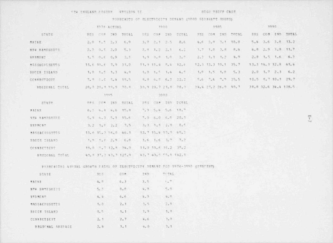
" EW ENGL AND P ECION VRcSIOT II HICit ?SICP CAST

TOPECASTS 07 EL ECT3ICI"Y OEM 4 50 (1003 GIG A'i ATT 00UR5)

1' 7 f A CTUA L 1930 1985 1990

STATE PES co? IND TOTAL ORS CDP IND TCTAL F!S C09 IND TOTAL RES COM IMD TOTAL

MAIEE 2. A 1.5 2.3 6.9 3. 7 2.1 25 8.6 4.6 2.A 3.1 10.8 5.4 3.6 3.8 13.2

NIW HaitSHIRE 2.3 1.5 2.0 5.3 2. 9 1. 2 2.1 6.2 1.7 1.0 2. R R.4 4.8 2. 9 1.9 11.7

VF1MONT 1. 5 0.( C. 9 3.3 1. 4 1. 0 1. 0 3." 2.3 1.1 1. 2 4. 9 2.8 1. 5 1.6 6.3

31SSAcatSETTS 11.6 10. f 7. 9 31.0 11.4 11.4 P. 4 12.6 12.3 12.3 10.1 35.7 13.3 14.1 12.9 41.4

EECtf ISLAMD 1. 8 1.5 1. 3 4.R 1. 9 1. '. 1.4 4.9 1.0 1. 5 1. 0 5. 3 2.0 1. 7 2.1 6.2

C C N K E CTICUT 7. 9 6.C 5. 4 19.5 9. 9 6.2 0.3 22.2 c.6 '.6 '.' 25.5 10.5 e. 7 10.1 29.7

BEGIONAL TCT%L 28.0 21. 1 19.9 70.A 30.9 21.7 21.8 78.1 34.4 27.2 26.9 90.7 38.8 32.6 34.4 10 R. 5

1945 2000

STtTE DPS CC' IND TOIAL R93 CDP IMD TCTAL

MnIEE 6.2 4.4 4.6 15.8 '. 0 5.4 5.6 19. '

1Eu MA1?SRIEE 5. 9 f6. 3 S.1 15.6 7.0 6.0 6.0 20.1 7w

YEPFCET 3. 2 1.E 2. 2 7.5 3. 3 1.9 2. 9 E.5

5ASSAC10S?TTS 13.6 15.3 16.0 46.1 12.7 15.4 19.9 49.2

SBCCE ISLAND 1.0 1.F 2. 9 6.9 1. 6 1.6 3. ' 7.2

CCNMECTICUT 11.0 a.7 12.9 34.0 11.0 10.F 1C.2 3 P. 2

BRCICNAL TOIAL 41.9 3'.2 43.7 125.9 42.7 41." '5.1 142.1

701ECASTED % :M U AL GPOWTH T A1 ES OF ELECTPICITY DE1\1r FCU 1476-1000 ( r ?RC E MT)

STATE RC S COM ISD Tf?AL

9 AIRE 4. 8 6.3 3.5 L.'

NPW HA9FSHI23 5. 2 8.P 4. 9 5.9

S F3 *C ET 4. 4 6. 6 4. 0 4. 9

9%SSACHUSETTS 1. 0 2.1 3. 5 2.1

RFCCE ISLAND 0. 5 1.1 1. 9 1. 4

CCN5fCTIC1T 2.1 2.7 4. 6 3. 0

R EGIC M AL AV EP A3 E 2. 4 3.1 4. 0 3.1

l

I

.

|; N EW ENGLAND REGION VERSION II HIC 3 PRICE CAS E

FORECASTS OF ELECT 3ICITY PRICE (? / 1000 KWRR)

19 7 E A CTU A L 1990 1985 1990

ETATE RES COP IND TOTAL RES COE IND TCTAL B ES C05 IND TOTAL RES COE IBD TOTAL

MAIRE 34.9 35. 1 19.4 2S.5 47.3 45.2 32.3 42.2 73.4 69.4 57.1 6 '. 5 101.7 96.6 84.8 95.3

REW HAMPSHIRE 45.6 48. S 29.6 40.1 6 2. 5 6 4. 6 C E.2 57.2 91.3 89.9 72.' 94.7 126.9120.4103.8 117.6

VERRORT 40.0 37.0 25.9 35.1 52.5 46.8 32.4 45.8 81.1 72.1 58.4 73.0 109.1 96.7 82.6 98.7

MASSACHUSEITS 40. 7 47.C 37.3 45.5 '4.6 67.5 56.1 67.2 120.3111.6 99.5 111.2 161.2154.2139.6 151.9

BECIE ISLAND 4 8. 2 43. C 3 6. 0 43.0 7 7. 3 71. 6 L ' . 8 71.8 11 E. 91 10. 9104. 4 110.8 165.0159.3153.2 158.84

CCNMECTICUT 44.7 41.7 33.2 40.5 63.7 61.6 47.6 58.4 102.9102.0 85.9 97.3 143.3145.8125.8 118.0

REGIC4AL AVERAGE 4 3. R 42. 1 30.2 3!.0 63.0 59.6 46.6 57.1 97.7 92.7 'o.7 90.8 134.5128.8115.0 126.7

1995 2000

STtTE RES CCP IND TOIAL RES CDP IND ICT1L

MAIEE 139.8134.2122.4 132.9 194.2189.0176.7 197.2

N EW HA9FSHIRE 195.6176.1158.1 173.R 2'0.7260.22?9.8 256.9 g1m

V E R EO NT 166. 9154. C 13 9. R 155.4 2 6 0.1249. 3 21E. 5 2 4 9. 2

MASSACHESETTS 2 57. 02 50. f 214.7 2 4 6.9 41R.8409.8395.7 406.3

'RFCIE ISLAN9 290.5274.?26o.1 273.9 4 9 2. 0 4 74. 74 '0. 2 4 7 4. C

CCN & E CTICHT 218.0224.3200.9 213.1 136.4345.6320.2 332.0

PECICTAL A7EEAGE 208.0202.3187.5 19 9. 3- 127.0321.4300.5 317.6

?,

FO REC AST E D 1F9 9 AL GPOWTH E AIES OF ELECTPICIT Y PRICE wnB 1776-1990 (DESC71T)

S1%IE RES CCM IND TC*AL

9AISE 7. " 7.5 11.1 E.'

WFW 561PSHITE 7. 6 6.7 9.4 a.0

VE9PCET 7. 4 7.1 9. 7 7.'

1ASSACHESETT7 8. 8 8.9 9.9 7. 0

RFCtE ISLAND 9. 2 9.9 10.0 C.9

CCNEECTICUT 8. 7 9.3 10.0 0.1 i

|

R EGIC 1 AL %VESAG' 8. 3 8.3 1 c. 0 a a I

_ - _ _ _

_

9:3'LS ATLANTIC F17IC4 VEESION !! 3ASE FDICS CASE

FOPECASTS O' EL ECT3 ICIT T DE* A ND (1300 GIG As ATT E0525)

19 7 f ACTU AL 1930 1995 1990

STATE EZS CCP TND TOTAL 2'S COM IND TCTAL FIS COM TMD TOTAL RIS CC? IND TOTAL

ETE YO5K 2" . 4 30. E 2 0. 6 99.3 32.6 34.5 30.' 108.2 2 a.0 45.1 2 a. " 134.9 44.6 59.0 49.1 168.8

MIS JEBSEY 15.1 14.2 15.9 45.6 19.2 17.4 1 e. 3 54.5 22.3 24.' 25.1 72.8 27.3 24.3 34.2 96.9

PERNSYLVANI\ 2R.R 17.5 43.4 91.9 34.2 21.1 48.2 105.( 41.4 29.6 61.4 135.1 49.4 40.2 77.3 170.3

FECICMLL TOT 4L ' 3. 3 63.C 9F.' 23(.9 95.0 71.0 97.2 269.3 101.* 9'.3125.4 342.0 121.3133.5160.5 435.9

s

1995 2000

-5TLIE 2ES CO? IND TCT%L R35 CDP IMS TCT4L

MfE Y3BK 49.4 73.4 62.8 205.7 54.6 90.5 RO.4 249.5m

NEW JIRSFY 32.2 46.5 26.4 126.4 37.6 62.5 62.1 164.c j,IEPNSYLVAN!t 56.7 51.2130.5 212.9 64.3 64.5131.1 265.E

SECICNAL TCTAL 13R.4171.~209.6 545.3 156.6219.0274.6 F9C.2

F03ECASTIE A 'N U A L ''R OW T H P A T IS OF ELECTRICITY DEMAN FCR 197f-1990 ( T ERC INT)

SitT E RES COM IMD TCTAL

NIH YORK 3. 0 4.9 3. 7 3. 9

N7E JfRSEY 4. 3 6.5 5. 7 5.5

FF)DSYLTAMT\ 3. 9 5.9 4. 2 4.5

R EGIC N AL AVEPA3R 3. 7 5.5 4. 3 4.5

_ _ _ _ _ _ - _ - _ _ _ _ _ ___ _ _ _ _ - _ _ _ _ _

._ - - - _ _ _ .

MID9 LE A TL ANTIC R EGION VERSION II BASE PRICE CASE

FORECASTS OF ELECTRICITI PRICE ($ / 1000 R3HR)

19 7E A CTU A L 1980 1985 1990

STATE RES COP IND TOTAL RES COM IND TCTAL RES COM IND TOTAL RIS COM IND TOTAL

Nfs YoBK 53.7 55. E 2 5. 5 45.1 69.9 73.3 44.9 63.3 10 0.61 C9.1 75.2 95.3 131.3147.5105.1 129.1

NEW JfRSEY 52.7 4R.2 33.2 44.5 67.1 66.4 50.6 61.3 98.0103.1 79.0 93.1 129.9147.5105.6 127.6

TE5NETLYANIA 41.2 38.0 25.7 33.1 55.6 50.0 37.7 46.1 7 e.8 74.4 56.7 67.6 105.2105.5 76.3 91.9

BEGICNAL AVERAGE 49.2 47.2 28.1 4C.9 64.2 63.2 44.4 56.9 92.4 95.2 70.3 R S. 3 122.2133.5 95.7 116.2

1995 2000

STATE RES CCE IND TCTAL RES COP IND TCTAL

NIE YORK 177.0205.3150.0 179.1 234.6286.9211.9 242.7

Y,Nfu JfBSEY 177.1219. E 14 5. 4 180.R 241.3327.6198.7 257.9 ro

PE5NSYLTANIA 138.0147.7101.3 122.7 18 0. 4 2 08. 013 3. 3 16 3. C

EPGICMAL AVERAGE 164.0199.E132.2 16C.9 220.4274.2191.3 223.4

FOR EC ASTED AT;U AL GROWTR R aiES OF ELECTRICTTY PRICE FOR 1976-1990 (P E RC' 5T)

51 ATE RES COM IND TCTRL

NIE YORF 6. 6 7.2 13.6 1.R

NEW JfBSEY 6. 7 8. 3 9. 6 7. 0

FF5NSTLVANTA 6. 9 7.6 R.1 7.6

PFGICNAL AVFRAGE 6. 7 7.7 9.1 7.'

- - _ - - ..

.. ..

_- _- - - _ _ _ .

9I99 LE \TL ANTIC "IGICT V ERS IO N II LCS PRICE C.\S!

FORECASTS O' EL ECTRICITY DEM4 5C (1003 GIq 1W ATT POU95)

19 7 ( ACTUAL 1990 1585 1990

ET&T! RES CC2 IND TOTAL EES COE IND TCTAL FYS COM IND TCTAL RIS COM IND TOTLL

MfW YORK 29. 4 30. E 2 9. 6 99.3 31.6 36.5 30.0 111.R 41.5 51.2 30.5 146.3 50.4 69.1 53.1 127.5

NEW JFPSPY 15.1 14.2 15.8 45.6 19.7 19. 4 1E.4 56.1 24.1 27.9 25.4 78.1 30.1 39.6 34.9 105.5

PENNSYLVANTA 2 9. a 1'.T 43.4 91.9 34.8 22.1 4 F. 4 137.5 43.6 22.R 62.1 141.4 53.0 46.1 73.5 191.4

BECICNAL TOTtL 73.3 E3.C 88.7 236.9 87.1 77. 1 97.8 275.4 109.2111.9127.0 365.7 133.5154.9163.4 474.4

1995 2000

ETATE EES CCP IND TCTLL RES COE IND TCTAL

NFE YORK 59.3 89.5 64.5 234.7 69.0112.1 93.2 292.27

NEW JEBSEY 36. 8 54. ' 47.6 140.3 44.7 74.3 65.1 192.1 sW

EEENSYLVANI% 62.3 60.7102.7 23C.4 72.7 79.7134.7 292.1

fECICBAL TOTAL 158.4202.1214.7 605.3 196.4265.1293.0 770.3

703 EC 4ST 7 0 A W U1L GROWT!! E ATES OF ELECTRICITY DE1LND FCR 1976-1090 ( FERC Y1T)

51%TE DES COM I1D TCTAL

NfW YCRK 3. 9 5.9 3. 9 4. 6

| N!W .1 t R S P Y 5. 0 7.5 5. 8 6. 2

F E b N 1 'I V 4 MI,\ 4. 5 7.0 4. 3 5.0'

i

REGIONAL AY?RA1E 4. 4 6.6 4. 5 5.1

h

_ _ . _ . . _ _ _ _ _ . _ _ - __ --. __--______________ - -____________________________ ______________ ____ - _ _ _ _ _ . _ ___ ___ _ _ _ _ _ . . _ _ _ _ _ - _ - _ _ . _ _ _ _ _ _ _ _ _

9IDDLE ATLANTIC REGION VERSION II LOW PRICE CASE

FORECASTS OF ELECTRICITY PRICE [$ / 1000 KWBR)

19 7 E A CTU A L 1980 1985 1990

STATE RES COP IND TOTAL RES COM IND TCTRL 723 COM IND TOTAL BIS COM IND TOTAL

NEE YORK 53.7 55.E 25.5 45.1 64.3 69.6 39.2 58.2 R3.0 94.7 56.9 79.7 104.3130. 0 76.1 106.5

5th JEBSEY 52. 7 49.3 33.2 24.5 62.4 62.6 45.5 56.8 83.3 92.6 62.2 79.7 108.1136.6 79.7 109.6

FEMNSYLTANIA 41. 2 39. C 2 5. 7 33.1 52.9 47.3 34.4 43.2 7 C.4 67.5 46.3 58.9 9 2.1 9 7. 9 5 9. E 78.9

bEGICMAL ATED103 49.2 47.3 28.1 4C.9 59.8 59.5 39.7 52.1 78.9 84.9 55.1 72.8 101.7121.5 71.5 98.3

1995 2000

STATE RES CCP IND TCTAL R P.S COP IMD TCTAL

NEW YCBK 126.2172.7 95.4 136.2 153.2232.7110.7 176.0tn

E!W JIRSEY 136.9200.1 95.8 147.6 173.4300.6113.2 203.4 hN

EE)NSYLVANIA 115.1137.2 70.2 100.6 143.4195.9 82.4 125.1

SEGICN%L AVEEASE 12 6.1170. C 9 7.1 129.2 156.6243.1104.8 169.5

YORECAST2D \ ?N ORL GPOWTH P .11ES OF ELECTRICITY PRICE F0F 1 '* 7 6 * C90 (PEDCENT1

SitTE RES COM IND TCTAL

MfW Y1RK 4. * 6.3 9.1 E.3

NEW JiRSTY 5. 3 7.7 6. 5 E.7

IFil!YLVANTA 5. 9 7.0 6.1 6.4

R EG IC 1 AL AVER AG? 5. 3 7.0 6. 9 E. 5

- - - _ _ _ - - - - _ _

"T331' ATLANTIC Rf0ICN 7EPSIO1 II PIGH ?'IC! C AS E

F0E! CASTS OF ELECTRICITY D2'4 4C (1000 GIGAWATT BOURS)

1776 RCTUAL 1990 1985 1990

S~ ATE PP.S Cd' IND TCILL R?S COM IMD TCTAL PES COM IND TOTAL RIS CC5 IND TOTAL

NEW YORK 29.4 30. E 2 9. 6 14.3 32.1 34.7 3 C. 7 107.7 35.6 45.2 39.7 132.2 40.4 60.3 49.8 165.3

EIE JIBSEY 15.1 14 . 3 15. P 45.6 17.9 17.5 19.3 54.1 2C.7 24.5 24.9 70.9 2 4. 5 3 4. R 33.9 94.1

PE5NSTIVANIA 28. 9 1'.T 43.4 11.9 33.9 21.3 of.2 105.5 34.4 33.3 61.4 134.4 46.P 41.6 77.1 169.9

FICICN4L TCitt 73.3 63.C RE.7 23E.8 83.7 73.5 97.2 267.3 7E.3103.n125.0 337.5 111.11J6.6159.7 429.2

1<95 2000

!*ATS RMS CCP IND TCTAL RSS CDP IND TCTAL

NYW TCSK 43.0 75.3 62.2 199.6 4 4. 2 93. 2 7 c.4 235.7rei

Els JERSFY 27.5 47,3 45.8 121.4 30.0 64.0 61.9 157.6 /.L.a

FPP5EYLVANIA 52.6 53.a100.2 210.5 5 9. 3 69.113 C.7 262.4

IEGICNAL TOT 4L 12 3.11'6.129 c. 2 5 3 2. 0 132.5225.1272.0 65c.'

FO R EC AST F S A V4 74 L G ROW T:f P \ T ES OP ELECTRICITY DEMA 4C FCR lo76-1970 ( F EPC EN T)

ST LT E B75 CCM IND TCTAL

NEW YORK 2. 3 4.9 3. 6 3. '

NfW JERSEY 3. 5 6.6 5. 6 5.1

TPl35YLVANIA 3. 5 6.2 4. 2 4.4

R FOIC1 AL AVER AO! 3. 1 5.7 4. 3 4. 3

|

_ _ - _ _ _ ______ __ --___ -_-_.__- -_ _. - _ _ . _ _ _ _ _ _ _ - _ _ _ _ _ _ _ _ - - _ _ _ _ _ _ _ _ - _ - _ _ _ _ _ _ _ - _ - - - . - _ - _ _ _ - _ _ _ _ . - - _ .

.

l ,

MIDDLE ATLANTIC BEGION YERSION II BIG 5 PRICE CASE

FOBEC ASTS OF ELECTRICITY PRICE ($ / 1000 KWRR)4

19 7 f A CTU AL 1980 1985 1990

STATE RES COE IND TOTAL RES COE IND TCTAL BES COM IND TOTAL RIS CO M IND TOTAL,

REE YORK 53.7 55.6 25.5 45.1 71.4 77.0 48.5 66.8 116.7124.7 91.7 111.6 158.4176.9133.1 157.6

BIE JIBSEY 52.7 48.3 33.2 44.5 71.2 70.8 55.0 65.6 115.9122.3 98.5 111.9 158.9181.3138.3 159.8

PEENSYLVANYA 41.2 39.C 25.7 33.1 57.1 51.5 39.5 47.8 85.3 E3.0 64.6 75.1 117.G122.3 91.0 106.2

BFGICNAL AVERAGE 49.2 47.3 28.1 40.9 67.3 66.6 47.7 6C.1 106.0110.0 84.9 99.6 144.8160,1120.8 141.2 ;

!

1995 2000

i STATE RES CCF IND TCTAL RES COE IND TCTAL

NEE YORK 239.0270.E212.7 242.9 361.0415.2335.9 375.1

NEW JIPSEY 2 4 3. 0 294. t 218. 7 25 4. 2 174.0479.9344.6 405.8z~

: EEINSYLVA4In 159.5179.5127.9 149.0 217.7261.317E.8 209.5

FEGILUAL AVE 3 AGE 213. 52 49. C 18 6. 4 215.4 117.6385.5286.4 310.1i !'

t.

..

!

703EC ASTEC A K4UAL GPOWTH P ATES OF ZLECTRICITY PRICE F09 1975-1990 (P E BCE s?) |'

STATE RES CCM I4D TCTAL

i

i Nf6 TORK 8. 0 0.6 12.5 9.3

NEW JEBSEY 8. 2 9. 9 10.7 9.6;

E ? n N S Y L V A N T .% 7. 7 0.7 9.4 E. '

|BE3ICNAL %YEPAGE 8. 0 9.1 11.0 9.1

,

. - _ _ - , , _ _ _ __ _ . _ .

_ _ _ _ _ _.

.

EAST NORTR CENTR AL REGION TE2 SICS II SASE PRICE CASE

FORRC ASTS OF ELECTRICITY D5 MAND (1000 GIJA VATT HOURS)

1976 ACTUAL 1980 1985 1990

STATE RES CO M IND TOTAL P ES CO M IND TOTAL RES C0 9 IND TOTAL RES COM IND IOTAL

CHIO 29.0 19.6 49.6 101.3 34.4 23.2 56.9 118.1 42.0 28.5 71.0 145.9 48.2 33.6 88.1 175.3

INDIA 4A 16. 6 9.3 24.7 51.1 20.0 11.1 29.1 61.1 24.2 13.7 37.8 76.6 27.7 16.2 48.3 93.3

ILLINOIS 26.1 22.4 33.3 88.i 29.3 25.9 35.1 96.8 34.1 29.7 41.8 113.3 38.6 33.3 50.8 131.5

MICHIGA4 21.1 13.5 31.1 67.8 24.3 15.8 34. 1 76.3 28.3 18.8 40.0 89.6 31.9 21.7 47.2 103.7

WISCOMSIM 12.4 8. 2 11.2 32. 8 14.4 9. 9 12.2 37.6 16. 8 11.8 14.6 44.5 19. 1 13.6 17. 8 52.1

REGION AL TOT AI 105.6 73.0149.9 341.0 122. 4 85.8167.6 390.0 145.4102.5205.2 469.9 165.5118.4252.2 555.91995 2000

STATE RES C09 IND TOTAL R ES CO M IND TOTAL

CHIO 53.4 18.3109.2 207.1 58.4 42.9135.1 244.2

INDIANA 30.7 1R.4 61.5 133.9 13.7 ?O.6 78.1 133.9tt

ILLIMOIS 41.4 35.9 60.1 147.6 43.3 18.1 71.6 164.0 j,w

MICHIGAN 34.2 23.5 54.6 115.5 35.7 2a.3 63.1 126.6

W I SCO N SI M 21.0 15.0 21.3 59.0 22.5 16.3 25.4 66.1

7 8GIO4 4L TOTAL 380.7333.2306.9 643.4 193.6142.2373.5 734.9

FO R EC ASTED A NN1 AL G POWTH D ATES OF RLECTPICITT DE9AMD FO R 1976-1990 (PEPCEMT)

SI AT E RES C )9 I ND TOTAL

CHIO 3.7 3.9 4.2 4.0 -

I49IANA 1.7 4.1 4.9 4. 4

ILIIN0IS 7. 8 7.8 3.1 2. 9

MICHI1AM 2.9 1. 5 3.0 3.1

W I SCO N S I4 3.2 3.6 3. 4 3.4

REGIOMAL AVFRAGE 3. 3 3. 5 3.8 3. 6

. - . _ . . _ _m_ ._ _ - - .

EtST NORT H CE*TR AL REGION VERSIO7 II 3ASE PRICE CASE

FORECASTS OF FLECTRICITY 2 RICE (f / 1006 KWHP)

1976 ACT U \L 1980 1995 1990v

ST4TE D'S CO" TM) T0 * .%L C ES Co * IND TOTA'_ EES COM IN3 TOTAL R RS CC9 IND TOTAL

OHIO 35.6 31.8 19. 7 27.2 41.8 4 2. . 27. 1 14.5 53.6 56.0 33.2 46.4 67.6 72.6 51.5 60.2

IMDIANA 30. 2 29.4 14.9 25.0 17.3 16.4 26.1 31.7 47.9 47.5 36.1 42.0 60.5 60.7 47.7 53.9

ItLIMOI" ?". 6 37.6 22.5 31.8 49.0 49.6 32.0 42.2 65.5 67.3 43.3 59.2 33.6 87.7 66.4 77.6

MICHIGAN 18.1 40.3 27.0 33.6 50.3 52.1 15.5 43.9 68.571.25s.5 62.2 38.7 92.4 73.4 92.3

VI SCO N S T M 14. 4 11.9 21.4 10.4 uu.9 44.0 31.8 40.9 61.7 61.L 50.4 57.8 79.9 80.8 68.4 76.1

"EGIrwtL A7FPAG? 15. 5 35.0 22.5 29.6 44.0 44.6 10.9 38.7 59.4 60.7 45.3 53.5 76.3 79.8 63.5 70.0

1995 2000

S?4TE PE9 C0 9 ING TOTAI P ES C09 IN3 TOT 4'

CNIn 81.0 90.7 66.4 75.4 302.7111.0 85.5 94.7

INDItMA 74.5 75.2 60.9 67.0 92.1 93.2 77.8 83.8Y

TIII!!OI S 108.1111.7 90.7 101.9 140.4147.4123.6 134.4 se

.1TC91GAw 116.9i21.0401.1 110.2 155.5 8 5 9. l i 39. 'i 148.1

WISC(TSI9 101.5105.3 9i.9 91.6 135.0117.4121.1 111.0

PRGICM4L 47FPEG? 97.2101.1 R2.2 40.8 125.2110. 1109.9 118.4

F07 EC 4 97 ED 4 4 M'I AL G PO W" H P AIES OP ELPCTRICITY PRICM FOP 1976-1990 (PERCENT)

SYL"E RES CO9 I ND TCT4L

CHIO 4.7 5. 6 7.1 5.8

IN3I4NL 5. i 5. 3 6.4 5. 6

ILLINDIS 5.7 6.2 9.0 6.6

91CHIG44 6.1 6.1 7.4 6.6

W I SC09 S I N 6.2 6.4 7.9 6.8

R'GIOM4L AV'R4GE 5.6 6.0 7.4 6.1

_ _ _ _ _ _ _ _ .

. _ _ -

EAST NORTH CE4 TRAL PECION VRRSION II LOW PRICE CASE

FOPECASTS OF EI ECTRICITY DE9 AND (1000 GIGABATT 900RS)

1975 %CTUAL 3980 1985 1990

STATE RES COM IND TOTAL R ES COM IND TOTAL PES CO M IND TOTAL R ES COM IN3 TO T AL

CHIO 29 . 0 19.6 49.6 101.3 15.f 23.6 59.6 121.8 44.0 29.9 78.8 157.5 52.3 36.7103.0 la8.1

IMDIANA 16.6 9.3 24.7 51.1 20.3 11.3 30.7 62.9 25.3 14.5 41.9 :'.7 29.9 18.0 56.5 105.6

I LT.IM OIS 26.3 22.4 33.3 88.1 10.3 26.6 17. 5 101.2 37.9 32.4 49.5 127.4 45.5 38.3 62.2 156.6

9ICHIGA4 21.1 11.5 31. 1 67.8 25.3 16.4 16.5 80.4 li.8 21.8 46.6 102.4 38.4 26.3 58.4 126.6

WISCOMSIN 12.4 8. 2 11.2 12.8 14.9 10.3 13.0 39.4 18.8 13.2 17.0 50.5 22.7 16.2 21.9 62.6

7EGICMAL TOTAL 105.6 71.0149.9 341.0 125.7 89.1177.2 405.7 157.8111.1232.8 520.4 183.8135.5302. 1 649.6

1995 2000

STATE RES COM IND TOTAL P. E S CO M IND TOTAL

CHIo 60.4 41.2134.0 245.0 68.9 49.9174.1 302.2

INDIA 4A 34. 4 21.4 75.6 112.9 19.3 25.0100.9 167. 1 m

UILLINOIS 52.9 44.0 79.2 189.9 60.9 50.1300.8 227.3

.11C RIG A4 45.1 31.1 73.2 151.7 52.5 16. 1 91.7 185.3

VTSCONSIM 26. 7 19.3 27.9 76.2 31.2 22.7 35.4 92.1

REGION %l TOTAL 219.5359.0189.8 796.7 252.8181.7502.9 973.8

FORECASTED ANNffAL GE097H PATES CF EIECTRICITY DE9 AN D POR 1976-1990 (PERCENT)

STATE RES CO" IND TOTAL

ORIO 4.3 4.6 5.4 4. 9

TMDILNA 4. 3 4.8 6.1 5.1

IL1INOIS 4.0 1. 9 4.6 4.2

"ICHIGAN 4.3 a.9 4.6 4.6

WISCONSIM 4.4 5.0 4.9 4.7

REGIONAI AVERAGE 4.2 4.5 5.1 4. 7

. _ _ - - - - _ - - _ _ - - . _ _ _ _ - - - - _ - _ - - _ - - - - _ _ _ _ - - _ _ - _ - _ _ - _ _ _ _ _ _ _ - - _ - _ _ _ _ - _ _ - _ - - _ _ - - _ _ _ _ _ _ _ _ _ _ - _ - _ _ ..-.__ _ _ - _ - - _ _ - - __ _ _ _ _ - .

E AST NORTH CENTRAL REGION TERSION II LOW PRICE CASQ

FORECA STS OF ELECTRICITY PRICE ($ / 1000 KWHR)

1976 ACTUAL 1980 1985 1990.

STATE RES COM IND TOTAL R ES COM IND TOTAL RES COM IND TOTAL RES Con IND TOTAL

ORIO 35.6 33.8 19.7 27.2 40.7 41.3 26.0 33.4 50.6 53.8 34.9 43.1 61.6 68.9 44.7 53.9

INDIANA 30.2 29.4 19.9 25.0 36.2 35.5 25.3 30.7 45.3 45.1 33.0 39.0 55.5 56.5 48.4 48.1

ILLINOIS 38.6 37.6 22.5 31.8 46.4 46.6 29.5 39.7 57.6 61.9 40.5 51.8 70.0 79.4 52.8 65.1

MICHIGAN 38.9 40.3 27.0 33.6 47.3 49.3 32.5 40.8 59.4 63.3 44.3 53.1 72.9 79.5 57.2 66.9

BISCO NSIN 34. 4 33.9 23.4 30.4 42.2 41.5 31.2 38.3 53.8 54.9 42.2 50.1 66.6 70.5 54.4 63.3'

] REGION AL AYER AGE 35.5 35.0 22.5 29.6 42.6 42.0 28.9 36.6 53.3 55.8 39.0 47.4 65.3 70.9 50.1 59.5

1995 2000

STATE RES COM IND TOTAL P ES CO M IND TOTALj

l CHIO 72.8 84.5 54.6 64.7 96.4103.0 66.7 77.5

INDIANA 65.9 68.1 49.8 57.0 78.4 81.8 60.1 67.8 91-

IIIINOIS 82.7 97.5 65.4 78.7 98.2119.7 81.1 95.2 00

MICHIGAN 86.6 96.1 70.3 80.6 103.3115.6 86.2 97.1'

WISCONSIN 39.7 86.8 66.9 76.7 95.6106.9 82.3 93.2

REGION AL AVER AGE 77.6 86.6 61.4 71.5 92.4105.4 75.3 86.1

i

FUR EC ASTED ANN 7 AL GROWTH R ATES OF ELECTRICITI PRICE FOR 1976-1990 (PER CEN T)

STATE RES COM IND TOTAL

CHIO 4.0 5.2 6.0 5. 0

INDIANA 4.4 4.8 5.4 4.8

ILLINnIS 4.3 5. 5 6.3 5. .i

MICHIGAN 4.6 5.0 5.5 5. 0

WISCONSIN 4.8 5. 4 6.2 5. 4

REGIC'eAL AVERAGE 4.4 5. 2 5.9 5.1

- - - - - _ - - - _ _ .

. _ _ _ -,

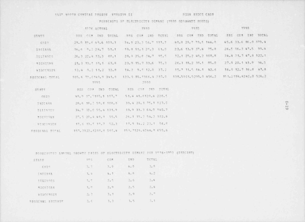
Y15? N0?TH CENT 2 AI R FGION V!RSTOM II H IS H E3ICS CASE

FOREC ASTS 0? ELECTRICITY DEP A5C (1000 GIG 8W ATT 00000)

19 ? f ACTUAL 1990 1S95 1990

STATE 22S CCF IND TOTAL R95 COP IND TCTAL PTS COM IND TOTAL REE CCM INC TOTAL

Ct!I O 29.0 19. E 4 9. 6 101.3 34.1 23.3 56.' 117.7 40.8 29.7 70.1 144.0 45.6 33.6 86.0 170.4

INCIA1A 16.6 0.3 24.7 51.1 19.9 11.1 29.3 61.0 23.6 13.9 37.4 75.8 26.5 16.3 47.5 91.4

.ILLINDIS 26. 3 22. 4 33.3 8F.1 29.9 25.P 34.7 95.9 32.1 29.2 40.2 108.9 34.4 31.7 47.8 122.1

MICHI1AN 21.3 13. ' 31.1 67.R 23.9 15.7 33.6 75.3 26.3 19.2 3A.1 RS.O 27.9 20.1 43.9 94.5

%ISCCNSIN 12.4 9.2 11.2 32.9 14.2 9.T 12.0 37.2 15.7 11.5 14.1 42.6 16.9 12.7 16.8 47.8

E EGIO N AL TOT AL 105.6 72.C140.9 341.0 12 3. 9 85. F 16 6. 4 237.0 13 8.51 C 1. 5 200. 0 456.2 151. ~ 114. 42 4 2. 0 5 26. 2

1995 2000

S*ATY RSS Cof IN D TOTAL - R CS C7E IND TCTAL

OHIO 49.9 37.7105.1 197.7 51.4 41.6128.4 222.5

INCIANA 28.6 1 A . 3 5 0. 8 100.0 30.4 20.1 75.1 127.C g16-4u)

IIIIN7IS 34.7 33. C 5 5. 4 131.9 11.9 33.3 64.0 140.7

91CH!"L1 2'. 5 20 . 4 4 P. 9 99.5 26.1 19.3 54.2 102.4

W I SC O N ST N 17.6 13 . ' 1".7 52.3 17.9 14.2 23.1 St.P

Y EGIC NA L T0* AL 157. 3122. F2 9 A. 9 5 9 t.4 151.7129.4344.9 655.4

70 3EC ASTED A NN UAL GROWTil D ATES OT ELECTRICITY D2MANC FCR 1076-19"3 ( F ERC INT)

sit 1E P93 COM IND TCTAL

CHIS 3. 3 3.9 4.0 3. 9

INDIANA 3. 4 4.1 4.R 4. 2

T I LI N 7IS 1. t 2.5 2. 6 2.4

11CHIGAN 1. " 2.4 2. 5 2. 4

WISCCNSIN 2. 3 3.1 2.9 2.'

RFGICNAL A7:nA7F 2. 6 3. 3 1. 5 3.1li

|

|

- _ - _ - _ _ - _ - _ - . - _ _ _ _ _ _ - - --____ - _ _ _ _ - _ - _ _ _ _ _ _ - - - - - _ - _ - _ _ _ _ _ - - _ - _ _ _ - - - _ -_ ,

E AS7 NORTH CENTR AI REGION VERS ION II HIGH FRICE CASE

FOREC ASTS OF ELECTRICITY PRICE ($ / 1000 KWHR)

197f ACTUAL 1980 1985 1990

STATE BES CCM IND TOTAL RES COM IND TCTAL FIS C05 IND TOTAL BIS C05 IND TOTAL

C9IO 35.6 33. E 19.7 27.2 42.3 42.7 27.6 35.1 55.5 58.3 40.3 48.5 72.0 77.4 56.3 64.9

INDIANA 30.2 29.4 19.9 25.0 37.4 36.8 26.7 32.1 49.4 49.3 37.8 43.6 63.6 64.4 51.4 57.3

IILINDIS 38. 6 37. E 2 2. 5 31.R 50.2 49.E 33.1 43.4 71.0 72.3 53.' 64.5 95.3 97.9 77.2 8R.7

MICHIGAN 38.9 40.3 27.0 33.6 51.9 53.7 37.1 45.5 75.5 77.8 60.3 69.0 133.4106.1 87.9 96.61'

WISCCNSIN 34.4 13 . ! 2 3. 4 30.4 46.1 45.1 35.0 42.1 67.1 66.8 55.8 63.2 91.8 92.1 80.4 87.8

BEGICN4L AVERAGE 35.5 35.C 22.5 29.6 45.6 45.6 31.9 39.6 63.7 64.9 49.6 57.8 E5.2 87.6 70.8 79.1

1905 2000

ST ATE RES CCP IND TOTAL RES COM IND TCTAL

OHIO 91.7 99.4 75.7 A4.4 117. 812 7. E 101. 6 110.3

I1DI AN A 80.6 82.1 68.0 73.8 102.9105.1 90.2 95.7,

C'IIIINGIS 130.9133.(113.2 123.7 1 R 2.1183. 9164.1 173.8

MICHIGAM 149.0151.3133.0 141.4 217.3218.9200.5 200.5

WI SCO NSIN 124.7125. 1113.1 120.3 171.6170.S15E.8 165.7

fECIC1%L AVEBAC? 115.4118.3100.6 10E.7 159.1161.3143.0 150.P

FOREC ASTEC 1N7 0&L GROWTH R t1ES OF ELECTRICITY PRICE FOB 1976-1990 (? Y BCM NT)

STATE BES COM IND TCTAL

CRIO 5. 2 6.1 7. 9 6.4

. INDIANA 5. 5 5. 8 7. 0 6.1

I I LI N9IS 6. 7 7.1 9. 3 7.6

MICHIGAN 7. 2 7.2 8. 8 7.R

WISCCNSIN 7. 3 7.4 9.2 7. 9

R FG IC N AL AVER 412 6. 4 6.8 8.5 7. 3

- -

_ _ _ - - -

.

UEST NORTH OENTE AL REGION VEES!3N II B A SE C AS

FORECASTS OF ELECTRICIt Y DEM.iND [1000 GIG AW AT" HCO25)

1976 ACTUAL 1980 1985 1990

STATE RES COM IND TOTAL R SS COM IND TOTAL RES COM IND TOTAL RIS COM IND TOTAL

9INNESOTA 10.7 4.8 11.9 28.2 13.1 6.2 15.4 35.8 16.2 8. 4 21.7 47.7 19.3 lu.6 29.3 6u.9

IOVA 8. 5 4.8 7.2 21.0 9.5 6.0 8.1 24.2 10.7 7. 8 10.8 30.1 11.7 9.7 14.4 36.8

MISSnURI 13.S 7.7 11.9 34.2 15.7 9.7 13.3 40.0 18.9 13.7 17.0 52.1 21.9 18.5 23.3 65.8

NCETF 'AKOTA 2. 0 1.3 0.6 4.1 2.2 1.6 0. 9 5.0 2.5 2.1 1. 4 6.3 2.7 2. 5 1. 9 7. 5

SOUT1 AKOTA 2.1 1.1 0.5 4.0 2.3 1. 3 0. 6 4.5 2.6 1. 8 0.8 5. 5 2.8 2. 3 1.0 6.5

ME3FtSMA 4. 8 4.0 2.7 12.2 5.6 5.2 3.1 14.7 6.6 7.1 4.2 19.0 7.7 9.3 5.7 23.9

KANSAS 6. 8 6.2 5.8 19.2 7.6 8.0 6.8 23.0 8.3 10.5 9.1 28.5 9.0 13.2 11.8 34.7

F EC f 0N A L TOT AL 48.4 29.9 40.5 122.9 56.0 38.0 48.3 147.1 65.8 51.4 65.7 189.2 75.1 66.0 87.4 236.3

tMINH

1995 2ub0

STATE FES COM IND TOTAL RES COM IND TOTA

9I?:NESOT A 22.3 12.4 38.7 75.7 25.5 14.2 51.2 93.7

ICWA 12.4 11.2 19.0 43.8 12.9 12.5 25.0 51.9

NISSOURI 24.8 23.6 30.4 81.5 27.9 29.4 40.0 100.6

'!OPUI 3AKOTA 2. 8 2. 9 2.5 8.7 2. 9 3. 3 3.1 9.8

SOU T!! DAFOTA 3. 0 2.8 1.3 7.5 3.1 3. 3 1. 6 e.7

MMBRASTA 8. 6 11.6 7.4 29.1 9.4 14.1 9. 7 35.0

K ANSA S 9. 5 15.7 15.0 41.1 9.9 18.2 19.2 48.5

REGION A L TOT AL 83.4 80.3114.3 287.4 91.7 95.1149.9 348.2

I

||

_ _ _ - . _ _ _ _ - . _ . _. . . _ _ _ . . - . . - - - . . _ _ .

FOREC ASTED ANNUAL GEOUTH E ATES OF ELECTRICITY D EM A N D FOR 1976-7990 (PERCINT)

STATE RES Co .* IND TOTAL

MIENESOTA 4.3 5.8 6.7 5. 7

ICWA 2.4 5.1 5.1 0. 1

MISSOURI 3.5 6.4 4.9 4. 8

NORTH DAKOTA 2.1 5.0 3.3 4. 4

SOUTH CAKOTA 1. 9 '.2 5. 3 1. 5

M!BRASTA 3. 3 6.2 5. 5 4. 9

KANSAS 2.1 5.5 5.1 4. 3

PEGIONAL A7ERAGE 3.2 5.8 5.6 4. 8

YwN

- - - . - - - . - - - _ . - .

t

WEST NORTH CENTRAL REGION TERS23N I2 BASE CASE,

FORECASTS OF ELECTRICITY PRICE [S / 1000 KNHR) ,

1976 Act3AL 1980 1985 1990

ST ATE PES COM I ND TOTAL RES COM IND TOTAL RES COM IN3 TOTAL RES COM IND TOTAL

MINNESOTA 33.3 35.2 23.6 29.4 43.0 44.8 33.2 39.0 60.4 62.8 48.0 55.1 79.3 83.9 64.3 72.7 ;

ICWA 36.1 36.8 22.2 31.4 47.8 48.2 33.0 42.8 66.7. 67.8 50.7 61.1 86.2 89.4 68.6 80.0

MISSOURI 35.1 34.4 23.5 30.8 45.0 44.5 34.4 41.3 60.6 61.8 49.9 57.1 78.4 83.8 67.8 76.1

NCRTH DAKOTA 30.8 28.5 26.7 29.4 42.0 37.9 38.2 39.9 60.1 57.0 56.5 58.1 78.7 77.7 74.7 77.3

SOUTR DAKOTA 31.5 34.6 21.6 31.1 41.7 42.8 31.5 40.6 56.8 57.7 46.7 '55.6 74.3 76.7 64.2 73.5

NEBPASKA 29.5 26.6 18.6 26.0 39.7 36.7 28.2 36.0 56.3 !5.7 42.8 52.9 74.4 77.8 57.8 71.7

K ANSA S 31.8 29.5 20.5 27.6 42.3 43.1 32.0 39.4 60.1 66.9 50.2 59.4 80.5 94.3 70.6 82.4

REGICYAL ATERAGE 32.6 32.2 22.4 29.4 43.1 42.6 32.9 39.9 60.1 61.4 49.3 57.0 78.S 83.4 66. 9 76.2,

YNLa

1995 2000

STATE RES COM IND TOTAL R ES COM IND TOTA * 2

MINMEscTA 104.1111.1 86.2 95.9 136.9146. 3115.7 126.4

IOVA 113.2118.7 93.8 106.0 149.6156.8127.8 140.6

MISS0nRI 98.2109.4 87.9 *6 123.5142.0113.8 125.1t

NCRTH DAKOTA 104.7105.9100.0 103.7 140.0143.2134.0 139.1T

SOUTH DAKOTA 94.0 98.8 83.7 94.0 119. 3127.4108.8 120.5,

!

NEEPASKA 99.0107.1 78.5 96.9 132.4145.4106.4 130.4

TANS 15 109.1129.3 99.2 113.3 149.0175. 2138.9 155.0 !

REGICNAL AVERAG2 103.2111.4 89.9 101.0 135.8148.0120.8 113.9 f

i

!

_ _ - _ _ . - --

FOREC A~T"3 AM40AL GECEIU R AT ES OF ELECTRICITT PRICE Fon 1976-1990 |PESCEKO)

S TA TE BIS COM IND TOTAL

MIMMESOT A 6.4 6.4 7. 4 6. 7

IOWL 6.4 6.5 8.4 6. 9

M IS SO URI S. 9 6.6 7.3 6. 7

NORTM 7AKOTA 6.9 7. 4 7.6 7.1

SrU"R E AKoit 6.3 5.9 8.1 6. 3

1'BFASTA 6. S 8.0 9.4 7. 5

KANS%S 6.8 8. 7 9. 2 8.1

REGION AL AV IP AGE 6. 5 7.0 9.1 7. 0

Ym5'

-- - _ - _ _ .

_ _ _ _ _ - ~ , . _ _ . _ . _ _ _ _ _ _ _ _ . _ _ _ _ _ _ _ _ - _ . _ _ _ _,

WEST NORTH CENTB AL REGION TERS!3N II L ON PRICE CASE

FORECASTS OF ELECTRICITY DEMAND (1000 GIG AW ATT H03RS)

q. 1976 ACTUAL' 1980 1985 1990

ST 4 T E RES C05 IND TOTAL RES CO3 IND TOTAL R25 C05 IN3 TOTAL R ES COB IND TOTAL '

NINNESOTA 10.7 4.9 11.9 2 8.~ 2 13.4 6.4 15.3 36.2 17.5 9.0 2?.1 49.0' 21.6 11.9 28.8 64.2,

IOWA 8. 5 4. 8 7. 2 21.0 9.8 6.1 8.1 24.7 11.6 8.4 10.6 31.6 13.3 11.1 14.4 39.9

MISS3URI 13.5 7.7 11.9 34.2 16.0 9. 8 13.2 40.2 20.0 14.3 16.9 52.9 24.0 20.2 22.2 68.5 .

'

NORTM D AKOT A 2. 0 1.3 0. 6 4.1 2.3 1. 6 0.9 5.1 2.7 2.1 1. 3 6. 5 3.0 2.7 1. 9 8.1

S OUTH D AKOT A 2.1 1.1 0. 5 4.0 2. 4 1. 3 0. 6 4.5 2. 7 1. 7 0. 7 5.5 3.0 2.3- 1. 0 6.7

N E3B ASK A 4. 8 4.0 2.7 12.2 5. 8 5. 4 3. 2 15.2 7. 3 7. 8 4. 3 20.4 8.8 10.7 5.9 26.9

KA4SAS 6.8 6.2 5. 8 19.2 7.9 8. 2 6. 9 23.5 9.3 11.3 9.1 30.3 10.7 14.8 12.2 38.6I

REGIONAL TOTAL 48.4 29.9 40.5 122.9 57.5 38.8 48.1 149.4 71.0 54.6 64.1 196.1 84.5 73.7 86.4 252.9

gs -a w

w1995 2000

STATE RES C01 IND TOTAL RES COM IND TOTAL

MINMESOTA 26.1 14.8 38.4 91.9 31.4 17.9 50.5 102.9i

1044 14.9 13.9 19.3 49.6 16.7 16.9 25.9 61.2

MISSOURI 28.1 27.1 29.7 86.5 32.6 35.2 36.7 108. 0

NORTH D AKOT A 3. 4 3.4 2. 7 9.9 3.7 4.1 3.6 12.1

SOUT4 D AKOT A 3.3 2.9 1. 3 9.0 3.6 3.7 1. 7 9. 6

NE3RASKA 10.4 14.2 8.2 34.6 12.3 18.5 11.4 44.5

KANSAS 12.3 18.9 16.1 48.3 14.0 23.7 21.1 60.2

| REGIONAL TOTAL 98.5 95.2114.6 318.8 114.3120.0151.0 398.5

,

_ _ _ _ _ _ _ _ _ _ _ __ _ ________ _ _ _ _ _ _ __ _ _ _ _ _ _ _ _ _ _ __ __ _ _ _ _

.. .-. . . . ~ . . - ..._ . _ , ,.

.

PORECASTED ANEGEL GROWTH RATES OF ELECTRICITY DE515D FOR 1976-1990 (PEBCEWT)

STATE FTS COM IND TOT &L

i

RIWNESOTA 5. 2 6. 7 6.5 6.1'

IOW& 3. 3 6.2 5.1 4. 7

RISSOURI 4.2 7.1 4.6 5.1

EORTH D&KOTA 3.0 5.6 8.3 5.0

SOUT5 D&KOTA 2. 4 5. 2 4.9 3. 74

BEBRESKA 4.4 7. 2 5.8 5.8

KAWSAS 3. 3 6.4 5.4 5.1

BEGIONAL AT EB&GE 4.1 6.6 5.6 5. 3

7mm

1

|

:

i

4

i

i

t

!

:

|

|

'

\

<

. - . v - -

- - ._ _ _ _ _ . _ - _ . _ _ _!

_ - _ _ _ _ _ _ _ _ _ _ _ _ _ _ - _ _ _ . . _ . _ - . _ _ _ _ _ _ _ _ - _ _ _ _ _ _ _ _ _ _ _ _ _ _ __ . . .. ._ _ _ _ _ _ _ _ _ _ _ _ _ _ _ _ _ _ _ _ _ _ _ _ _ _ _ _ _

WEST NORTH CENTR AL REGION YE SS IO N IX LOW PRICC CASE

FORECASTS OF ELECTRICITY PRICE ($ / 1000 KWHR)

1976 ACTUAL 1980 1985 1990

STATE RES COM IND TOTAL RES COM IND TOTAL RES CO M IND TOTAL RES- COM IND TOTAL

MIWNESOTA 33.3 35.2 23.6 29.4 40.6 42.3 30.7 36.6 52.9 55.8 40.4 47.9 67.1 74.0 50.8 60.9

IOWA 36.1 36.8 22.2 31.4 44.8 45.2 29.9 39.8 57.5 59.0 41.3 52.3 71.6 77.2 52.9 66.3

MISSODEI 35.1 34.4 23.5 30.0 43.3 42.8 32.6 39.6 55.2 56.8 44.3 52.1 68.7 76.5 57.3 67.3

NORTH DAKOTA 30.8 28.5 26.7 29.4 39.2 34.9 35.2 37.0 51.1 47.5 46.7 49.9 64.3 63.6 58.8 62.7

SOGTH DAKOTA 31.5 34.6 21.6 31.1 40.2 41.3 29.9 39.2 52.5 53.1 42.0 51.2 66.0 67.7 55.2 65.0

NEBRASKA 29.5 26.6 18.6 26.0 36.6 33.7 24.9 33.0 47.6 48.1 33.1 44.6 60.3 67.7 40.5 58.8

KANSAS 31.8 29.5 20. 5 27.6 39.0 40.4 28.7 36.4 49.6 59. 2 39.3 50.1 61.6 83.2 50.7 66.6

REGION AL AVER AGE 32.6.32.2 22.4 29.4 40.5 40.1 30.3 37.4 52.3 54.2 41.0 49.6 65.7 72.9 52.3 63.9

YNN

1995 2000

STATE RES COM IND TOTAL R ES C05 IND TOTAL

MINNESOTA 82.2 95.0 61.2 74.4 130.9121.0 74.2 91.0

IOWL 86.0 99.1 64.1 80.7 103.4124.5 77.3 98.1

MISSOURI 82.8100.7 70.7 94.4 130.0132.2 87.1 106.3

NORTH L AKOT A 77.8 81.7 69.8 76.9 94.1104.7 81.6 93.9

SOUTH DAKOTA 79.7 84.7 68.3 79.8 96.5107.0 84.0 98.5

NE8RASKA 73.7 91.2 45.7 74.3 90.2121.9 48.3 92.7

KANSAS 74.0111.1 61. 8 84.7 89.3146.8 74.8 107.2

REGIONAL RVERAGE 79.4 94.7 63.1 79.7 96.3122.6 75.3 98.2

.

-- -. -_ _ . - . _ _ - ~ .

'FOBBCASTED A555AL GROWT5 B ATES OF ELECTRICITY PRICE FOR 1976-1990 (PF2CENI)

> STATE RES C05 IND TOTAL!, |-

MIENESOTA 5.1 5.5 5.6 5. 3 |

IONA S.0 5. 4 6.4 5.5;

NISSOURI 4.9 5.9 6.6 5. 7,

1 -

| NORTH D&KOTA 5. 4 5.9 5.8 5. 6:4 SOUTR DAKOTA 5. 4 4. 9 6.9 5. 4

NEBRASKA 5.2 -6.9 5.7 6.0

KAESAS 4. 8 7. 7 6.7 6.5+-

, REGIONAL ATERAGE 5.1 6. 0 6.2 5. 7! t

j .

1 t

*A

J

tN

i CD

i

r

L

i

i

l

!.4

!

E

,

i

_ _ . . _ _ _ _ _ - _ _ _ _ . _ ___ _ _ - -

._

_ . _ . _ _ . , _ - _ _ _ _ _ _ _ _

>

r

WEST 503T8 CGBTRAL RQGZON VERSI3N KI HIGH PRICE C AS E

FORECASTS OF ELECTRICITY DEMAND (1000 GIGAN ATT BOU RS)

1976 ACTUAL 1980 1985 1990

STnTE RES COM IND TOTAL RES C05 IND TOTAL RES COM IND TOTAL R ES C05 IND TOTAL

MINNESOTA 10.7 4.8 11.9 28.2 13.0 6. 3 15.8 36.2 15.7 8.7 23.4 49.3 18.2 10.8 34.1 65.1

IoW A 8. 5 4. 8 7. 2 21.0 9.4 6.2 8. 7 25.0 10.3 8. 7 13.4 33.2 11.0 11.3 23.2 43.7

MISSOURI 13. 5 7.7 11.9 34.2 15.7 10.1 14.4 41.4 10.7 15.4 22.3 58.3 21.3 21.9 32.6 78.2

NORTE D AKOT A 2.0 1.3 0.6 4.1 2.2 1. 6 1. 0 5.1 2. 4 2. 4 1. 8 6. 9 2. 5 3.0 2. 6 8.5

SOUTH DAKOTA 2.1 1.1 0. 5 4.0 2.4 1. 4 0. 6 4.7 2. 6 2.2 1. 0 6.3 2. 9 3.1 1. 5 8.0

N EBRLSK A 4.8 4.0 2.7 12.2 5.5 5. 3 3. 3 14.9 6.1 7. 5 4.9 19.5 6.6 9.8 7.1 24.7.

KANS%S 6.8 6. 2 5. 8 19.2 7.4 0. 2 7. 2 23.3 7. 4 10.9 10.3 29.3 7. 4 13.5 14.0 35.7

REGIONAL TOTAL 48.4 29.9 40.5 122.9 55.5 39.1 51.1 150.7 63.2 55.7 77.2 202.8 69.8 73.4112.0 264.0

toIMM3

1995 2000

STLTE RES COM IND TOTAL RES COM IND TOTAL

5INNESOTA 20.6 12.8 50.7 86.7 23.1 15.0 77.8 119.4

IOW4 11.3 13.3 30. 1 56.1 11.2 14.7 45.0 73.0

MISSOURI 23.8 28.6 47.3 103.0 26.4 36.3 70.1 137.1

NORTH DAKOTA 2. 5 3.5 3.4 10.0 2.5 4. 0 4. 5 11.6

SOUTH D AKOT A 3.0 4.0 2.0 9.6 3.2 4. 9 2. 7 11.5

NEBRASKA 6.8 11.9 9. 8 30.1 6.9 13.8 13.7 36.3

KANSLS 6.8 15.2 18.2 41.1 6.1 15.8 23.3 46.3

REGIONAL TOTAL 74.8 89.2161. 5 336.6 79.4104.6237.0 435.3

_

PORBCASTED 4550&L GROSTE ' R&TES OF ELECTRICITY DER &BD FOR 1976-1990 (PERCEET)

STATE RES COR IND TOTALi

i

RINEESOT& 3.9 5.9 7.8 6. 2

1054 1.9 6.3 7.7 5. 4

NISSOURI 3.3 7.7 7.5 6.1

50RTF D&KOTA 1.6 6.4 10.5 5.3

SOUTH D&KOT A 2.1 7.6 8.1 5. 0IF

NEBB&SKA 2. 2 6. 5 7.2 5.2

*

KkNS&S 0.6 5.7 6.5 4. 5

R EGIO N A L &TER&GE 2.7 6.6 7.5 5.6

t:1ItoO

!

F

9

i

_ _ _ - . . _ . ..

- _ - _ _ - - - - . .- ~. . _ . . . _ _ . . . . . --

WEST NORTH CENTRAL REGION VE RS I3 N II HIGH PRIC3 CAS E

FORECASTS OF ELECTRICITY PRICE ($ / 1000 KWHR)

1976 ACTUAL 1980 1985 1990

STATP- RES COM IND TOTAL R ES C05 IND TOTAL RES CO M IND TOTAL RES C05 IND TOTAL

{ MINNESO7A. 33.3 35.2 23. 6 29.4 24.2 45.9 34.0 39.9 65.2 66.2 51.7 59.1 89.6 95.2 71.0 80.5

IOWA 36.1 36.8 22.2 31.4 49.2 49.7 33.8 43.8 74.5 76. 9 55.3 67.2 99.8107.1 73.3 89.1'

NISSOURI 35.1 34.4 23.5 30.8 45.9 45.5 35.3 42.0 64.5 68.0 53.6 61.2 86.1 98.8 74.9 85.0

NORTH DAKOTA 30.8 28.5 26.7 29.4 43.8 39.8 40.1 41.7 68.4 67.8 65.1 67.3 94.8 99.9 90.1 95.2

SOUTH DAKOTA '31.5 34.6 21.6 31.1 41.9 42.8 31.9 40.7 57.7 60.5 47.9 57.0 75.9 85.'s 65.4 78.0

N EBR A SK A 29.5 26.6 18.6 26.0 42.3 39.5 30.5 38.5 68.6 69.5 53.7 65.0 100.21C6.5 79.5 96.6

KANSAS 31.8 29.5 20.5 27.6 45.5 46.7'35.3 42.7 77.1 85.3 67.3 76.7 116.9132.3107.0 118.9

RE3IONAL RVERAGE 32.6 32.2 22.4 29.4 44.7 44.3 34.4 41.3 68.0 70.9 56.4 64.8 94.7103.7 80.2 91.9

A'

ysuPd

1995 2000

STATE RES C05 IND TOTAL R ES COM IND TOTAL

MIMMESOTA 122.4131.5 95. 2 107.4 168.2182.1124.5 140.6

IONA 140.0152.0101.8 121.9 198.2213.2138.7 163.6

MISSOURI 110.6135.3 99.0 112.2 142.7182.5130.3 147.0

NORTH DAKOTA 136.1146.2128.9 137.3 196.8211.7185.1 197.5

SOUTH DAKOTA 97.7117.5 86.2 103.9 126.1159.4112.6 137.9

NEBRASKA 150.5161.4120.8 144.8 228.4242.5183.4 216.2

KANSAS 197.4214.5186.5 198.9 337.9351.1325.1 335.9

REGION AL AVER AGE 136.4151.2116.9 132.3 199.8220 4171.4 19 1. 2

.[

|4

_ _ _ _ _ _ _ _ _ _ . _ . _ .

. . . _ _ . . _ . _ . . _ . ~ _ . ~~ .m__ _ __ . . . _ - . _ _ . . .- ....s ._ . .. .....m __ - . _ _ _ . . . _ . . . . . .

FOREC&STED ABUS&L GROWTE R ATES OF ELECTRICITI PRICE FOR 1976-1990 (PERCE BT)

ST&TE BES C05 IND TOTAL

HINNESOTA 7. 3 7.4 8.2 7. 5

10s& 7. 5 7.9 8.9 7.7

EISSOURI 6.6 7.8 8.6 7. 5

NORTH D&KOTA 8.4 9.4 9.1 8.8

SOUTR D&KOTA 6. 5 6.7 8.2 6.8

I WEBRASKA 9.1 10.4 10.9 9. P

KANS&S 9.7 11.3 12.5 11.0

REGIONAL AT ER&GE 7.9 8. 7 9.5 8. 5

!

<

wN

i

_ _ - _ _ . _.. . _ _ - _ _

_ . _ _ _ _ _ _ _ _ _ _ _ _ _ _ _ __ - - - . . . - - . _ _ _ _ _ _ _ _ _ _ _ _ _ _ _ _ . _ _ . . - -.. . . . . . . .

. -- _ _ _ _ _ _ _ _ _ _ _ . . -

SOUTH LTLANTIC REGIOM VERSION II S ASE CASE

FORECASTS OF ELECIaICITY DEE AND (1000 GIG AWATT HOURS)

1976 ACTUAL 1920 1985 1990

STATE RES CCM IND TOTAL RTS COM IND TOTAL BES CO M IND TOTAL RIS CO M IND COTAL

'.3 7. 2 6.5 2.5 1. 7 3.9 8.2 3.2 2.2 ~4. 9 10.43!LAVARE 1.6 S.2 2.6 5.4 1. 9 1

M APYL AND AND D. C. 11.C'10.9 13.5 36.0 13.0 11.5 20.2 45.5 15.7 13.4 27.1 57.2 19.2 16.3 33.6 70.4

YIRGINIA 16.7-11.0 9.7 41.7 20.4 13.0 10.7 49.3 25.1 16.0 12.5 60.0 30.9 20.2 15.2 74.1

WEST VIPGINIA 5.1 3.0 9.9 18.1 6. 5 3.9 12.4 22.9 8.3 4.9 15.4 28.7 10.1 5. 9 18.7 35.0

40PTH CAROLINA 20.a 11.9 20.4 54.1 25.1 14.5 22.7 64.1 31.6 18.4 27.2 79.4 38.9 23.3 34.0 98.8

S0078 CAROLINA 10.4 6.1 14.8 32.2 13.1 7.6 16.3 3 8. G 16.3 9.4-19.4 46.4 20.1 11.7 24.5 57.8

1;.512.214.6 45.7 21.5 14.3 16.3 52.5 26.5 18.7 19.4 65.1 33.0 24.9 23.8 82.58GE0EGIA

FLCEIEA 55.0 21.2 14.2 73.3 42.9 26.1 15.5 86.9 57.2 36.2 18.1 114.6 78.0 51.0 22.1 155.3

F!GIONAL TOTAL *19.6 77.4 99.7 306.6 144.2 92.3117.4 365.6 183.2118.6143.1 459.5 233.5155.6176.7 584.3 mi

1995 2000

STATE RSS COM I ND TOTAL R ES 00M IND TOTAL

DELAWA9E 3. 9 2. 6 6.0 12.6 e.5 3.1 7. 3 15.0

M AF YL AN D A N3 3. C. 22.4 19.3 40.1 83.3 25.4 22.3 46.9 96.3 ,

VIRGINIA 36.3 24.4 18.5 88.6 41.7 23.1 22.3 104.1

WEST VI9GI NI A 12.1 6.9 22.6 41.8 14.4 8.0 27.1 49.7

NORTH CAROLINA 45.3 27.5 42.0 118.0 51.2 31.3 51.3 137.5

S001H C AROLIN A 23. 3 13.5 3s.9 69.6 26.3 15.2 38.7 82.4

GF0FGIA 38.9 31.1 28.9 99.8 44.7 37.9 24.6 118.2

FLORIDA 98.2 65.3 27.1 195.9 118.2 73.3 32.9 236.8

R!GION4L TOTAL 280.5190. 8216.1 709.7 326.4226. 1261.1 840.0

- . . . , . . . . , . . _ _ _ _ _ ___. _ _ _ _ _ _ _ _ _ _ _ _ _ _ _ _ _ _ . _ _ _ _ _ . _ _

___. . _ _ _ _ _

FOR EC AST ED ANNU AL GROWTH R ATES OF ELECTRICITY DEMAND FOR 1976-1990 [PER C ENT)

STATE RES COM IND *iOT A L

D EL A W A R E 5.4 4.5 4. 4 4. 7

94RTLAND AND D. C. 4.1 3.0 6.7 4. 9

7IBGIRIA 4. 5 4.4 3.3 4. 2

WEST TIBGINIA 5. 0 4.9 4.7 4. 8

NOFTH CAROLINA 4. 7 4.9 3. 7 4. 4

SOUTR CnR3 LINA 4.8 4.7 s. 6 4. 3

GEORGIA 4. 2 5.2 3.6 4. 3

FloBIEA 5.7 6.5 3. 2 5.5

REGIONAL AVEPAGE 4. 9 5.1 4. 2 4. 7

Y%

_ - _ _ _ _ _ _ _ __ _

SOUTH AT* A5!IC P.EGIO N YEESYON 17 SASE C ASS

PG3ECASTS OF ELEOISICITY PFICE (3 / 1000 KWHE)

1976 ACTUAL 192 u 1995 1990

STATE P2S COM IND TOTAL R ES COM ISD TOTAI BES CCM IND TOT A L R ES CO M IND TOTAL

DELABA?E 45.? 41.4 28.9 36.4 58.J 54.3 41.5 49.2 81.4 79.1 64. 0 72.6 106.1106.1 96. 3 96.8

M AT YL A43 AN3 D. C. 52.7 53.5 17.4 47.1 70. u 6 7. 8 5 3. 6 6 2. u 100.6101.0 81.5 91.5 '130.4135.8107.0 120.3

VIPGINTA 35.1 34.2 22.9 31.7 47.7 47.2 24.7 44.4 69.5 69.9 E4.6 66.2 92.5 94.1 73.7 88.7

V?ST VIRGITIA 35.9 34.2 21.8 27.9 44.2 41.4 30.2 36.* 59.3 56.1 43.3 49.8 75.1 73.6 58.2 65.7

NCPT3 CLFOLTMA 32." 29.0 21.4 27.8 42.7 36.6 29.6 16.5 59.9 51.6 44.7 52.6 78.u 66.5 59.6 68.7

5007.9 CAE0 LINA 33.1 29.5 19.3 25.9 43.2 37.7 28.6 35.6 69.5 54.8 43.7 52.5 30.9 72.8 57.6 69.1

GEORGIA 29. 3 35. F 2 3.1 29.0 40.4 46. 4 ? 3. 2 39.8 59.3 66.5 50.7 58.8 80.7 89.6 68.6 79.9

FI OFI O A 36. 7 37.8 27.1 35.1 Ss. 2 51. 8 3 9. 8 48.9 75.8 73.1 66.1 7 5. w 102.01uu.3 92.1 1u1.5

*EGIC4AL AV3 FAG 2 17. 6 37.0 25.2 12.6 29.5 47.9 36.4 44.0 70.8 69.6 56.1 64.9 93.2 92.9 75.4 86.3Yuw

'995 2000

STA22 E23 C09 IND TOTAL 3ES COM IND TOTAL

3?LA7A9E 142.*144.G12v.1 1Yt.0 191.2194. 9167.4 130.3

MAFYLAN) AND D. T. '73. 5184.4145.3 1(2.3 231.8249.1198.5 219.4

VIPGI51A 12 5. 9 ' 2 3. 510 3. u 121. 5 17 u. 917 4. 714 4. 9 165.3

WEST VIRGINIA " ?. 6 9 2. f 74.2 32 .9 117.5116. 7 94.6 104.8

NCBTN CAFOLI51 luu.4 90.2 83.9 93.5 139.7123.0197.9 127.4

SOUTH CAROLI"A ' 08. 310w.1 8 0. 3 94.1 146.1137.0112.1 128.0

GEOFGIA *13.2'23.9 99.3 112.2 157.917u.4140.8 156.9

PLCFIDA 144.4147. 4136.4 144.3 204.'6207.8200.8 205.2

P.2GIC N AL A?!EAG2 925.8126. 4105.2 117.9 170.0171.7147.1 161.0

-- - ._.___ _- . - . . - -

FOREC ASTED A NNUAL GROUIH R ATES OF ELECTRICIIY PRICE FOR 1976-1990 (P E3CE NT)

STATE BES Co.1 IND TOTAL

DELAWARE 6. 3 7.0 8.1 7. 2

M AR TL AN3 A N3 D. C. 6.7 6.9 7.8 6. 9

YIRGIBIA 7. 2 7.5 8. 7 7. 6

WEST VIRGINIA 5.4 5.6 7.3 6. 3

NORTS CAROLINA 6.4 5.9 7. 6 6. 7

SOUTH CAROLINA 6.6 6.7 9.1 7. 3

GEORGIA 7.5 6.8 8.1 7. 5

PLOPIDA 7. 6 7.6 9.1 7. 9

R EG IO N& L AVIPAGE 6.7 6.8 8.1 7. 2

#

_ _ _ _ __

. _ _ _ _ _ _ - - - = _ _ _ - - - . - -- _ _ _ _ - _ _ -

|

SO9'!! ATL ANTIC REGIO N VEFSION II LCW ' 22IC2 CASE

FORECAS;S OF 2LECIRICIT Y DEM AMD (1000 GIG 3WAT! IICURS)

1976 ACTUAL 1980 1985 1990

ST %T R . RES CO* IND TOTAL CBS 001 IND TOTAL CIS 005 IND TOTAL RIS CO M IND TOTAL

DYL4W ARE - 1. 6 1. 2 2.6 5.4 2.o 1. 4 ' 3. 2 6.7 2. 9 - 2. 0 4.1 9.1 ' 4.0 2. 7 5.4 12.2

M AR YL AN D A 43 D. C. 11.0 10.9 13.5 36.0 '3.7 12. 1 20.6 4 7. - 18.5 15.6 29.1 64.3 24.3 19.9 37.9 83.7

714GIEI4 16.7 11. C 9.7 41.7 21.4 13. 7 11.C 51.5 28.6 13. 3 13. 4 67.6 3(.9 24.1 17.0 87.2

WES! VIRGINIA 5.1 1. 0 9.9 18.1 6. 7 4.0 12.6 23.3 9.0 5. 4 16.0 3J. 5 - 11.6 6.9 20.0 38.7 i

MCET!! C AROLIM A 20.4 11.S 2 0.4 54.1 25.9 15.2 23.0 65.9 34.6 21.1 28.5 d 6. 5 44.1 28.4 36.6 112.2

SOUIH C1ROLIMA 10.4 6.1 14.8 32.2 13.5 8.0 16.5 39.1 17.9 13.7 20.5 50.4 22.8 13.8 26.8 65.2

G90RGIA 18.5 12.2 14.6 45.7 22.4 14. 9 16.6 54.4 29.7 21.0 20.4 71.8 38.8 29.0 26.0 94.7

FLCFIEA 36.0 21.2 14.2 73.3 45.5 27.9 15.9 91.8 67.9 43.7 13.5 134.7 98.8 65.9 25.1 195.0

REGIONAL TOTAL 119.6 77.4 99.7 306.6 151.0 97.3119.3 379.8 239.2127.7151.6 515.0 281.519u.7194.7 688.7YwN

194 5 2000

STATE RES CCM IND TO! AL PE9 COM IND TOTAL

DELAVAE3 5.2 1.5 7.0 15.8 6. 6 4.4 9.0 20.3

M A9YL AND AND D. C. 30.6 24.1 47.9 105.1 37.6 30. 3 59.8 130.3

VIRGIRIA 46.0 30.8 21.7 110.2 56.8 39.3 27.8 138.5

WEST VIRGINI1 14.4 8.3 24.7 47.7 17.7 9.9 30.4 58.3

UOR7:t C AROLIN A 54. 6 37. G 4 7.1 142.6 66.9 47.7 60.7 180.2

SOPT!! C AROLIN A 28.2 17.3 35.8 83.5 34.5 21.3 49.1 107.8

G'OPGIA 49.1 38.7 33.0 121.9 61.3 53.9 42.0 155.5

| FL"SID% 137.1 93.( 32.4 270.4 187.2130. 8 42.0 369.9

[ PEGIONAL TOTtt 365. 3254.0249.6 897.1 468.9334.6320.81160.8f

||

|

_- . .. _ _ _ _ . _ _ _ _ _ _ _ _ _ _ _ _ _ _ _ - _ _ _ _ _ _ _ _ _ _ _ = _ _ _

_ _ _ _ _ _ - _ - - _ - _ _ _ _ _ _ _ _ _ _ _ - _ _ _ _ _ _ _ _ _ _ _ _ _ _ _ _ _ _ _ _ _ _ _ _ - _ _ _ - _ _ _ _ _ _ _ _ _ . _ _ _ . _. . _ _ _ _ - _ _ _ _ _ _ _ _ _ _ _ _ - _ _ _ _ _ _ _ _ - - . _ _ _ _ . _ _ _ _

FOR EC AST ED ANMU AL GROSTE R ATES CF ELECTRICITY DEM%ND FOR 1976-1990 ( P!E CINT)

STATE RES COM IND T OT A L

DEL 4 WARE 7. 0 6.1 5.2 6.0

M AP YL AN 3 A ND D. C. 5. 8 4.4 7.7 6. 2

VIRGINIA 5.8 5. 8 4.1 5.4

WEST TIRGINIA 6. 0 6.0 5.1 5. 6

NCETH C AROLIN A 5. 7 6.4 4.3 5. 3

SCDIH CAROLINA 5. 7 6.0 4.3 5. 2

GEORGIA 5. 5 6.4 4. 2 5. 3

FLCEIEA 7.5 8.4 4.2 7. 2

R EGICN AL AYERAGE 6. 3 6.6 4.9 6. 0

?uO)

i

__

- _ _ _ _ _

SOUTR %TI ANTIC F2GIO N YEISION II LCW 2EICE C102

FORZCASIS OF ELEC;RICI!Y P3 ICE ($ / 1000 EWHE)

197f 4CTUAL 1980 1985 1990

ST\T! RES COM IND TOTAL E93 CON IND TOTAL EIS COM INO TOTAL RIS COM IND TOTAL

D'L AW A13 45.3 41.4 28.9 36.4 51.1 Ss.9 37.4 45.1 68.7 63.6 49. 3 54.8 83.1 92.9 62.1 77.4

5)FYL%13 LUD D. C. 52.7 51.5 37.4 47.1 64.6 63.5 47.8 56.9 03.2 23.a 61.1 74.2 1v 6. 5119. 6 74. 2 94.3

VI:GI5It 35.1 34.2 22.9 31.7 44.4 44. 5 2 G.5 41.1 60.5 62.4 41.4 56.9 80.9 84.7 53.1 76.0

WES VIRGINIA 35.9 24.2 21.3 27.9 42.6 39.9 28.4 34.4 53.9 52.1 37.5 45.0 68.0 67.5 47.5 57.2

NCRTS C4EOL 4A 32.9 29.8 21.4 27.0 40.9 34.5 27.3 34.5 54.5 45.0 36.7 46.1 71.4 57.3 47.0 59.5

SM'7H C A?nLIN A 33.1 29.5 19.3 25.9 41.3 35.6 26.0 33.5 56.0 43.7 34.7 45.5 73.5 64.9 42.9 58.0

GEORG71 29.3 35.6 23.1 29.0 37.9 44.0 30.1 37.2 52.2 59.9 40.4 51.1 71.1 61.1 51. 8 68.9

F;OIICA 36.7 37.8 27.1 35.1 45.6 47.3 34.4 44.2 61.9 (4.4 47.9 60.6 82.0 85.8 62.9 81.2

P2GICNAL A739AG3 37.6 37.0 25.2 32.6 46.4 45.0 32.7 40.9 61.4 E 1.1 43.6 54.9 80.3 81.6 55.2 71.7?La@

199 5 2GGG

ST \! E RES Co r IND T O'. A L '25 COM IND TOTAL

DE;RWAr? 109. 6117.7 74.4 95.8 136.5150.1 89.1 118.1

M AP YL L3 0 AMD D. c. 132.3155.9 15.3 116.2 16 5.12w3. 0 97. 3 142.3

VIEGIK!A 103.9109.3 64.3 97.0 133.3142.2 77.2 123.5

9?r? VIRGINIA 83.8 84.0 57.1 70.0 1J3.71uu.5 69.0 85.7

NOT7H CAROLIMA 89.6 70.3 57.2 73.4 112.5 86. 3 69.4 9v.4

SOPTH C4h0LI4A 93.1 82.7 48.4 71.2 117.u105.3 50.8 83.7

GECF1It 92.8105.5 63.3 88.8 12v. 9137. 3 77.1 114.3

FLCBIta 105.1107.0 78.1 102.7 132.9134.7 96.7 129.4

E FGI CN ti A7EEAGE 101.3104.2 66.0 89.4 127.7132.9 78.3 ~10.9

.

- - -_

FORIC ASTED ANNUAL GROWTH R ATES OF ELECTRICITY PRICE [0R 1976-1993 (P EEC E RT)

S T AT E RES COM IND TOTA L

DELABARE 4. 9 5.9 5.6 5. 5

.1 AR TL A3 3 A NJ D. C. 5.1 5.9 5. 0 5.1

VIRGINIA 6. 2 6.7 6.2 6. 5

UEST VIRGINIA 4. 7 5.0 5.7 5. 3

MORTH CAROLINA 5.7 4.8 5.E 5.6

SCU"R C AROLIN A 5.9 5.8 5. 9 6. 0

GEOEGIA 6. 5 6.1 6.0 6. 4

FLOPIIA 6.0 6.0 6.2 6. 2

REGIONAL AVERAGE 5.6 5.8 5. 7 5. 8

>O

iw ,

_ _ _ _ _ _ _ _ _ - _ _ _ . _ . _ . _ _ _ _ - _ - _

- - - _ - - _ _ _ . . , , . _ _ - . -

SOUTH ATLANTIC REGION YERSION II HIGH PEICE CASE

FORECASTS OF ELECTRICITY DEMAND (1000 GI3ANATT EDURS)

1976 ACTUAL 1980 1995 1990

STATE R ES COM IND TOTAL RES C05 IND TOTAL BES C05 IND T3TAL R ES COM IND TOTAL

DELAWAR3 1. 6 1. 2 2.6 5.4 1.9 1. 3 3.1 6.4 2. 3 1. 5 3. 7 7. 5 2.7 1.8 4. 4 9.1

1 ARYL ANO AN D D. C. 11.0 10.9 13.5 .35.0 12.. 11.2 20.1 44.8 14.5 12.3 26.0 53.7 16, 4 14.4 31.3 63.7

V IRGI NI A 16.7 11.0 9.7 41.7 19.8 12.6 10.6 48.1 22.5 14.2 11.8 54.2 26.1 16.9 13.7 63.5

WEST TIRGINIA 5.1 3.0 9. 9 18.1 6.4 3. 8 12.4 22.8 8.1 4.7 15.2 28.1 9. 7 5.6 18.1 33.6

NORTH CAROLINA 20.4 11.9 20.4 54.1 25.0 14.4 22.6 63.7 31.0 17.7 26.8 77.5 37.5 21.7 32.9 94.7

S037H CAROLINA 10.4 6.1 14.8 32.7 13.0 7.5 16.2 37.8 16.0 9.0 19.0 45.3 19.4 11.0 23.6 55.4

GEORGIA 18.5 12.2 14.6 45.7 21.2 14.2 16.2 52.1 25.3 17.8 18.9 62.5 30.7 23.2 22.7 77.3

FLORIDA 36.0 21.2 14. 2 73.3 41.6 25.3 15.3 84.5 50.7 31.6 17.1 102.2 64.4 41.5 20.2 129.5

BEGIONAL TOTAL 119.6 77.4 99.7 306.6 141.8 90.3116.5 360.1 170.3108.8138.4 431.0 207.5136.2166.9 526.8

Y.sP*

1995 2000

STATE RES COM IND TOTAL RES COM IND TOTAL,

DEL AW ARE 3.0 2.0 5.2 10.2 2.9 2. 0 6. 0 10.9

M ARYL AN D AN D D. C. 18.3 15.9 36.0 71.5 18.8 16.8 40.3 77.3

V IR GI NI A 28.0 18.6 16.0 70.0 28.2 15.3 18.3 73.6

U EST TIRGIN Z A 11.4 6.5 21.6 39.6 13.3 7.3 25.6 46.5

NORTH CAROLINA 40.9 23.4 39.5 106.8 41.8 23.3 46.1 114.3

SOUTH CAROLINA 21.1 11.7 28.7 63.2 21.4 11.7 34.1 69.1

G EORGI A 33.5 27.0 26.7 88.0 34.2 29 2 30.4 94.8

FLORIDA 71.1 46.0 23.5 144.5 71.1 45.7 26.9 147.5

REGIONAL TOTAL 227.4151.2197.2 593.9 231.8155.3227.7 634.0

i

_ _ _ _ _ _ _ _ _ _ _

FOR ECLSTED ANNU A L GBOWTH R ATES OF ELECTRICIIY DE5AND FOR 1976-1990 (PERCENT)

STLTE RSS CO P. IND TOTAL

D EL &W AR E 4.1 3. 2 3.8 3. 7

ihRYLAND AN7 D. C. 3.1 2. 0 f.2 4. 2

VIRGINIA 3.3 2.1 2.5 3.0

W ES T WIRGINIA 4.7 4. 5 u.4 4. 5

NORTH CAROLINE 4.5 a.4 3.5 4.1

SOUTH CAROLINA 4.5 4. 3 3.4 3. 9

GEORGIA 3. 7 4.7 3.2 3. 9

F LOR I D A 4.2 4.9 2.6 4.1

REGIONAL AV E3 AGE 4.0 4.1 3.7 3. 9

Y>N

_ _ _ _ _

. _ _ _ - _ _ _ _ _ _ _ _ - - . _ . ._ ___ ___ _ _ _ _ _ _ _ _ _ _ _ _ _ _ _ - _ _ _ _ . . .. ..

. . . , _ . . . . _ -_ -_ _ - _ _ _ _ _ _ _ _ _

SOUTH ATLANTIC QEGION VERSION II HIGH PRICE CASE

FORECASTS OF ELECTRICITY PRICE ($ / 1000 KNHR)

1976 ACTUAL 1980 1985 1990

ST ATE RES COM IND TOTAL RES COM IND TOTAL RES C05 IND TOTAL RES COM IND TOTAL

DELAWARE 45.3 41.4 29.9 36.4 62.1 58.1 45.7 53.2 99.9 96.3 83.3 91.0 135.9133.4118.6 126.9

1 ARYL AND AN D D. C. 52.7 53.5 17.4 47.1 73.9 71.3 57.6 65.8 118.8117.2100.8 109.5 160.7162.1140.2 150.8

VIRGINIA 35.1 34.2 22.9 31.7 51.3 50.5 38.7 48.0 85.6 84.7 72.9 12.2 118.6118.3104.8 115.2

W EST VIRGINIA 35.9 34.2 21.8 27.9 45.5 42.7 31.5 37.4 63.1 60.6 48.2 54.6 84.0 82.1 67.9 75.0

NORTH CAROLINA 32.9 29.8 21. 4 ' 27.8 44.2 38.1 31.1 38.0 65.3 57.1 50.6 58.2 87.3 76.3 70.2 78.6

SOUTH CAROLINA 33.1 29.5 19.3 25.9 44.7 39.1 30.2 37.2 67.2 60.5 50.1 58.4 90.6 82.7 69.2 79.6

G EO RG I A 29.3 35.6 23.1 29.0 42.2 49.2 35.2 41.7 67.2 74.2 59.5 66.9 93.9102.4 84.0 93.6

| FLORIDA 36.1 37.8 27.1 35.1 54.4 56.0 44.4 53.1 95.5 97.7 87.6 94.8 135.5138.4129.7 135.6

REGIONAL AVERAGE 37.6 37.0 25.2 32.6 52.3 50.5 39.3 46.8 82.8 81. 1 69.1 77.0 113.3112.0 98.1 106.9

YS-w

1995 2000

STATE RES COM IND TOTAL RES COM IND TOTAL

DELAW AR E 214.'s211.6196.9 204.8 344.3340.9327.8 334.6

N ARYL AN D AN D D. C. 238.3241.7216.1 227.7 357.0361.3334.0 345.7

VIRGI NI A 184.8184.4171.5 131.3 291.7290.8280.0 288.2

, W EST VIRGINI A 107.6106.0 89.7 97.6 138.7137.3118.8 127.4

NORTH C AROLIN A 130.0118.4113.6 121.2 197.6187.1184.0 189.8

SOUTH CAROLINA 135.9128.1113. 2 123.8 207.5200.7185.4 195.1

GEORGIA 149.1158.5139. 6 149.1 239.1248.5231.6 239.6

FLORIDA 233.0236.4231.6 233.9 400.8411.1410.9 408.9|

REGIONAL AVERAGE 174.1173.1159.0 167.4 272.8272.2259.0 266.2

I

_. _ - _-_- _____-- - _ _ . .- - - _ - - - . -- _- -- ~-

FORBC&STED 1955&L GRONTE R ATES OF ELECTRICITY PRICE FCE 1976-1990 (PERCEBT)

STATE RES C05 IND TOTAL

D EL &W &B I 8.2 8.7 10.6 9.3

R &RYL AND AWD D. C. 8.3 8.2 9.9 87

TIRGIBI& 9.1 9.3 11.5 9. 7

WEST TIRGINIA 6.3 6. 5 8.4 7. 3

NORTE CAROLINA 7.2 7.0 8.8 7.7

SOGTE CAROLIsa 7.5 7- 9.5 8. 4

G EORGI A 8. 7 7. 8 9.7 8. 7

FLORID & 9.8 9.7 11.8 10.1

REGIONAL &V ERAGE 8.2 8. 2 10.2 8.9

Y>>

!|

. -.-- . . _ . . _ _ . . . - . . - - - - - - . - - - - - - - - - . - - - - - - -

EAST SOUT E C2FTR AL RECICN Y29SI05 IY B ASE PRICE CASE

FOB 2 CASTS OF 2LECTRICITY DEQAND (1000 GYGAVATT BOURS)

1976 ACTUAL 1980 1985 1990

STATI RES COM IND TOTAL RES C0 5 IND TOT AL RES C0 5 IND TOTAL R ES __2 IND TOTAL

KENTUCKY 10.7 10.2 15.2 37.3 14.1 12.1 17.8 45.4 18.9 14.9 24.5 60.2 24.1 18.1 32.6 77.2

TENNISSEE 23.6 3.9 32.6 60.7 27.6 5.7 39.1 73.2 34.4 8.3 51.5 95.2 42.5 11.3 66.6 121.E

ALAEAMA 14. 8 6.5 24.1 45.8 17.7 9.4 28.5 56. 1 22.3 13.7 37.0 73.5 27.4 18.6 47.1 93.9

EISSISSIPPI 8.2 4.7 7.2 20.7 9.2 5. 8 8.5 24.1 11.5 8.0 10.9 31.2 14.5 10.E 13.9 40.2

REGICNAL TOTAL 57.4 25.3 79.2 164.5 68.7 33.0 93.9 198.8 87.1 44.9123.9 260.2 108.5 58.8160.1 332.9

1995 2000

STAIE RES COE IND TOTAL R ES C0 5 IND TOTAL

KEN 13CKY 28.6 20.7 41.0 93.1 33.1 23.4 5 C. 8 110.7 ma

TENNESSEE 49.2 13.3 80.0 144.9 56.3 15.0 97.2 170.3 6;

AIAEAMA 31.4 22.6 56.6 111.7 35.3 2E.6 67.6 130. 6

MISSISSIPPI 16.8 12.8 16.5 47.2 18.8 14.6 19.5 54.1

REGICNAL TOTAL 126.0 69.5194.9 396.8 143.4 79.6235.1 465.7

i'

,

j

F09 fC ASTED ANNU AL GNONTH R ATES CF ELECTRICITY DEMAND FOR 1976-1990 (PEBCENT),

ST ATE RES COM IND TOTAL

KENTUCKY 6.0 4.2 5.6 5. 3

TENNISSEE 4.3 7.9 5.2 S.1

AIAEAMA 4.5 7.8 4.9 5.3

R.SSISSIPPI 4.1 6.1 4.8 4.9

BEGICNAL ATIBAGE 4.7 6.2 5.2 5.2

i

i

_ _ _ _ _ _ - _ - - - - - - _ - _ _ _ _ _ _ _ _ _ _ _ _ _ _ _ _ _ - _ _ _ _ _ _ _ _ _ - _ _ _ _ _ _ _ _ _ _ _ _ _ _ - _ _ _ _ _ _ _ _ _ _ _ _ _ _ _ _ _ _ _ -

EAST SOUT E CENTR AL REGICE YEBSICE II BASE PRICE CASE

PCRECASTS OF ELECTSICITY PRICE ($ / 1000 KERB)

1976 4CT U AL 1980 1985 1990

STATE' BES COP IND TOTAL RES COM IND TOT AL RES COR IND TOTAL RES CCE IND To:ll

KENTUCKY 26.2.16.7 10.8 20.4 32.8 28.1 29.7 30.3 44.3 41.6 41.1 42.3 57.9 56.6 53.1 55.5

TENNESSEE 23.0 27.2 18.6 20.9 31.1 34.4 27.0 29.2 46.6 46.3 40.9 43.5 64.4 59.5 55.9 59.2

AL4EAMA 27.6 30.3 18. 3 23.0 35.9 37.8 26.4 31.3 50.2 51.2 39.9 45.2 65.8 65.6 54.0 59.8

HISSIRSIPPI 37.3 33.1 23.8 29.1 44.8 45.9 37.4 42.4 64.2 65.1 57.3 62.0 85.9 86.3 78.9 83.5

REGICNAI AffBAGE 27.0 26.8 19.9 23.3 36.2 36.6 30.1 33.3 51.3 51.0 44.8 48.2 68.5 67.0 60.5 64.5

1995 2000

STATI RES COM IND TOTAL R ES CO E IND TOTAL

7 i

KERTCCKY 18.0 76.8 71.2 14.6 105.5103.9 96.4 100.8|n

"'

TENNISSEE 51.5 83.2 81.1 84.9 129.3117.8117.5 121.5

AIAEAMA 90.1 88.6 77.4 83.3 123.9121.0110.6 116.4l

MISSISSIPPI 123.2123.0116.1 120.6 177.6176.7170.4 174.7

BEGICNAL ATIRAGF 55.7 92.9 86.5 90.9 134.1129.8123.7 128.3

FCE! CASTED ANNUAL GEONTH R ATES CF ELECTRICITY PRICE FOR 1976-1990 (PERCEN T)

STATI RES CCM IND TOTAL

KENTOCKY 5.8 9.1 7.7 7. 4

TENNISSEE 7.6 5.8 8.2 7.7

AIDEAMA 6.4 5.7 8.0 7.0

MISSISSIPPI 7.5 7.1 8.9 7.8

EEGICNAL AVERAGE 6.9 6.8 8.3 7. 5

L_____._____ . .

.. . . . . . . . . ...

, . , . ._ . _

_ - _ _ _ _ _ _ _ _ - _ _ _.

. . - _ _ . . _ _ _ _ _ _ _ _ _ .

EAST SOUTH CE%TR AI REGION V!RSIO4 II 107 PRICE CASE

FOREC ASTS OF ELECTRICITY D!5 A ND (1003 GIC AW ATT H032S)

197E ACTUAL 1980 1995 1900

STATE RES COM IND TOTAL RMS COM IND TCTAL P!S COM IND TOTAL RIS CO M IND TOTAL

KINTUCKY 10.7 13.2 15.2 37.3 14.6 12.8 19.0 4 7. c 20.7 17.1 29.5 6R.4 27.5 22.0 42.4 94.9

1EB1?SSEE 23.6 3.5 32.6 60.7 29.7 6.4 42.0 70.0 37.6 11.1 61.0 110.7 47.9 17.0 97.0 153.4

ALABAMA 14.8 6.! 24.1 45.9 14.5 10.4 21.1 60.5 24.0 1'. 3 4 5. ' 9 9. ' 22.0 25.9 66 . R 125.'

MISSISSIPPI 8. 2 4.7 7.2 20.7 10.0 6. 8 9.4 26.8 13.7 11.0 13.5 39.1 18.3 1(.7 19.0 55.4

SEGIONAL TOTAL 57.4 25.3 70.2 164.5 71.9 36.5191.5 213.2 06.9 56.4148.' 3 0'. c 12 5. 7 e 1. 0 21% . 2 4 29. 4

1995 2000

STATE RES CO? IND TCTAL P95 CDP IND TCTALtM

KENTUCKY 34.8 27.5 62.5 128.8 43.3 34.3 99.9 183.3 [ ,

wT E N4 ESS EE 59. 3 24.112 0. R 20 6.3 73.1 33.2167.3 276.4

PLABAMA 39.6 36.2 96.1 173.4 48.6 49.7142.8 243.1

MISSISSIPPI 23.6 23.8 26.2 75.4 30.0 33.5 36.1 101.9

B ECTON AL TOT AL 157. 3111.7305.6 593.9 195.0150.6446.1 aog.7

FOREC ASTf D A NN UAL GROWTH R ATES OF ELFCTRICITY DSP.A 4D FOR 1076-1990 ( F?PC Y1T)

STATE RES COM I4D TOTAL|

KFNTUCKY 7. 0 5.6 7. 6 6.9

1E31ESSEE 5. 2 11.1 7. 3 6. n

ALABAMA 5. 7 10.4 7. 5 7. 5

MISSISSIPPI 5. 9 9.5 7.2 7. 3;

REGICN AL AVER AGE 5. 8 8. 7 7.4 7.1

_- - _ _ - _ _ _ _ _ _ _ _ _ _ _ _ _ _ _ _ _ _ _ _ _ - _ _ _ _ _ _ _ _ _ _ _ _ _ _ _ _ _ _ _ .

BAST SOUTE CERTR AI REGIO 5 YERSION II LOW PRICE CESE

FORRCASTS OF ELECTRICITY PRICE ($ / 1000 KWRR)

19 76 ACTU A L 1980 1985 1990

STATE RES COE IND TOTAL RES COB IND TCTRL R ES COM IND TOTAL BIS C05 IND TOTALv

KIN 10CKY 26.2 16.7 18.8 20.4 31.2 27.6 28.2 29.0 39.7 40.4 35.8 38.2 50.9 56.2 42.5 48.3

1ENNESSEE 23.0 27.2 18.6 20.9 29.5 31.8 25.0 27.3 42.1 39.9 34.4 37.5 57.9 48.7 44.7 49.3

ALABAMA 27.6 30.3 18.3 23.0 33.7 35.4 23.7 28.8 43.8 45.0 30.5 37.1 56.2 57.7 36.6 46.1

EISSISSIPPI 31.3 33.1 23.8 29.1 39.4 40.6 32.3 37.2 51.4 53.1 44.5 49.5 66.1 69.1 57.6 60.0

BEGICNAL AVERAGE 27. 0 26. E 19. 9 23.3 33.5 33.8 27.3 30.6 44.3 44.4 36.3 40.6 57.8 57.9 45.3 51.9

1S95 2000

STATE RES CCE IND TOTAL RES COB IND TCTAL

KINT0CKY 63.7 73.S 46.1 57.1 80.3 96.9 40.5 61.1 T's~'

1EENESSEE 75.8 60.3 55.1 61.7 99.1 75.9 67.8 77.1

ALAEAMA 70.2 72.0 41.0 54.2 88.1 90.7 42.2 61.4

MISSISSIPPI 82.3 86.7 70.4 79.5 10 3. 410 5. 7 R S.6 49.0 3

REGICN AL AVERAGE 73.0 73.2 53.1 63.2 92.7 93.3 59.0 74.7

FOREC ASTED ANMUAL GROWTH R ATES OF ELECTRICITY PRICE FOR 1976-1990 (P ERCE NT)

STATI RB S C09 IND TCTAL

KFMTDCKY 4. 9 9.1 6. 0 6. 3

1 E NMISS EE 6. 8 4.3 6. 5 6. 3

ALABAMA 5. 2 4.7 5.1 5.1

9ISSIGSIPT 5. 5 5.4 6.5 5. 8

REGICMAL AYLO A- " 5. 6 5.7 6.1 5.9

- _ _ _ _ _ _ _ _ _ _ - _ _

--. _ . __ _.

. _ _ _ _ - _

IAST SOUTH CENTR 41 R EGION YERSION II BIGH PRICE CASE

FOREC ASTS OF ELECT 3ICIT Y DEE4 ED (1003 GIG AWATT EquRS)

19 7 E A CTU AL 1980 1995 1900

ST 4T E RES CCE IND TOTAL RES COE IND TCTAL RTS COM IM7 TOTAL RES COM IND TOTAL

KINT0CKY 10.7 10.2 15.2 37.3 14.1 12 3 1 P. 5 46.3 19.5 15.6 26.7 A 3. 0 23.4 10.1 36.R 91.9

1EN9ESSEE 23.6 3.9 32.6 60.7 27.3 5.S 40.1 74.0 3 2. ' 9.4 64.4 96.6 79.6 11.2 '1.1 123.1

ALAEAM4 14.8 6.5 24.1 4 5. R 17.6 9.7 29.5 57.3 21.6 14.4 40.0 76.R 26.1 19.7 51.9 48.5

MISSISSIPPI 8. 2 4.~ 7.2 20.7 8.8 5. 6 E.5 23.5 9.0 7.0 10.7 29.3 11.6 T.0 13.5 34.0

BEGICsAL TOT AL 57.4 25.3 79.2 164.5 67.7 33.5 96.7 201.1 82.R 45.4132.1 264.6 100.6 59.0173.3 338.4

1995 2000

ETLTE RES CCE IND TOTAL RES COE IND TCTAL7

KfRTUCKY 2 5. R 20.E 44.6 94.1 27.2 21.3 52.' 104.4 -

e

1EsMESSEE 42. 5 11. E 8 2. 9 13 8.5 43.6 11.5 94.8 151.4

ALAEAMA 28.0 22.2 60.5 111.7 28.8 23.6 69.5 122.9

MISSISSIPPI 11. 0 0.0 15.1 36.9 11.4 8.5 16.6 37.4

RECION?L TOTAL 108.1 63.7203.1 381.1 111.0 64.9233.5 416.1

FOREC ASTED A NM DAL GROWTH R AT ES OF EL ECT RICITY DEMgMC FCR 1976-1900 ( F ERC ENT)

S14TE RES COM IND T CT 4L

( K E1 TUCK'T 5. 7 4.6 6.5 5. 8

1ENNESSEE 17 7.9 5. 7 5. 2

ALABAM4 4. 1 8.2 5. 6 5.6

EISSISSIPPI 2. 5 4.7 4. 6 3. R|

| BEGICTAL AVERAGE 4. 1 6.2 5.9 5. 3

_ _ _ _ _ _ _ _ _ _ _ _ _ _ - _ _ _ _ _ _ _ _ _ _ _ _ _ _ _ _ _ _ _ _ _________ _______ _ _ _

_ _ _ - _ - _ - _ _ _ - _ - _ _ - - - _ _ _ _ _ - _ - _ _ _

| EAST SOUTE CENTR AL REGION TERSION Ik HIG E PRICE CLSE

FOREC ASTS OF ELECTRICITY PRICE ($ / 1000 KWER)

19 7 6 A CTU AL 1980 1985 1990 -

STATE RES C05 IND TOTAL RES COE IND TCTAL E ES COM IND TOTAL RES C05 IMD TOTA L

KINTDCKY 26.2 16.7 18.8 20.4 33.9 29.5 30.8 31.4 48.4 e6.9 45.2 46.6 64.7 65.7 59.7 62.6 p

1ERWISSEE 23.0 77.2 18.6 20.9 32.7 36.1 28.9 30.9 53 54.0 48.8 50.8 76.1 73.4 69.9 72.2

ALAEAMA 27.6 30.3 18.3 23.0 37.3 39.1 27.6 32.6 55.8 57.0 45.1 50.4 75.6 76.4 63.5 69.3

BISSISSIPPI 31.3 33.1 23.8 29.1 J. 0 51.1 42.5 47.5 86.4 87.2 79.3 93.8 124.5125.*117.8 122.0 j

5ECICEAL AT!BAGE 27.0 26.8 19.9 23.3 39.5 38.9 32.4 35.6 61.0 61.3 54.6 57.9 85.2 85.2 77.7 91.5

i

1995 2000

STATE RES COE IND TCTAL RES COM IND TCTALm

K15TUCKY 98.7 99.8 92.8 9 5. R 152.9151.2146.7 149.3 2 !.

IC)

1EEMISSEE 123.4120.1118.4 120.2 203.0201.5200.6 201.4

311B151 116. 1116. 1104.5 109.7 181.0180. 4170.5 174.9

EISSISSIPPI 217. 4 217. E 210. 6 214. 7 382.9393.5375.9 379.8i

3ECIC41L AVERAGE 138. 9139.4131.6 135.1 230.0229.1223.4 226.4+

|

| '

i

!FOREC AST!D ANM UAL GROUTH R ATES OF ELECTRICITY PRICE FOR 1976-1900 (P E FCE WT)'

L

SIATI RES CCM IND TCTAL |

KIMTOCKY 6. 7 10.3 9.6 9. 36

i 1EN4ESSEE 8. 9 7.3 9.9 9. 3i

11ABAMA 7. 5 6.8 4. 3 ?. 2

FISSISSIPPI 10.4 10.0 12.1 10.8

BEGIC1AL AYERAGE 8. 5 8.6 10.2 1. 3

i

. , - - - + -, ,. _ _ ,.--

-

CEST SOUTB CENTR AL REGION TERSION II BASE CASE

FOR EC A STS O F ELECTRICITY DEM A N D (1000 GIGAunTT HO3RS)

1976 &CT U AL 1980 1985 1990

STATE RES COM IND TOTAL RES COM I5D TOTAL RES COM IND TOTAL RES COM IND TOTAL

ARKANSAS 6.7 41 6. 5 17.8 7.4 4. 8 7.9 20.7' 9.4 5. 7 10.4 26 2 12 2 6.6 13.7 33.5 j

LCUISIANA 13.4 81 19.5 44.2 15.7 10.3 20.3 49.8 18.212223.5 58.1 21.7 13.8 29.5 69.9

OKLAHOMA 9.4 6. 5 7.2 2:4. 5 11 3 8. 2 8.5 29.7 12 8 9.6 10.6 35.1 15 2 10.7 13.8 42 1

TEIAS 41.4 33.7 57.3 136.5 51 3 43.0 70.6 169.9 62 7 52 4 87.5 208.6 78.8 61 1108.5 256.0

REGIONAL TOTAL 70.9 52.5 90.5 223.0 85.7 66.3107.3 270 1 103 1 79.9131.9 328.0 128.0 92 2165.5 401 5

1995 2000

STATE RES COM IND TOTAL R ES CO R IND TOTAL

ARKANSAS 14.6 7. 2 18.0 41.0 17.0 7.6 23 5 49.4

LCUISIANA 25.0 13.0 37.7 83.6 28.3 15.9 48.6 99.8

OKL AHOM A 17.7 11 6 17.8 50.1 20.2 12.4 23 1 59 1

TEIAS 95.9 69.6133.7 308.4 115.5 77.6164.3 368.3

REGION AL TOT AL 153 2103.5207.3 483 0 181 0113 3259.5 576.5

FORICASTED ANNU AL GROUTR RATES OF ELECTRICITY DEM AND FOR 1976-1990 (PEBCENT)

STATE RES COM IND TCTAL

ARKANSAS 4.4 3.5 5.5 4.6

LOUISIANA 3.5 3.9 3.0 33

OKLAHOMA 3.5 3.6 4.8 3. 9

TEX AS 4.7 43 4.7 4.6

| REGIONAL ATERAGE 4.3 41 4.4 4.3

!

.

. . .

__ _ _ _ _ _ _ _ _ _ _ _ _ _ _ _ _ _ _ _ _ _ _ _ _ _

. . - _ - - _ - _ - - _ _ . - - _ - _ _ _ - _ _ _ _ _ . _ _ _ .____._ - ___-_ -

WEST SoWTE CENTRAL REGIOR TERSIOR II ''.SE CASE

FORBCASTS OF ELECTRICITI PRICE ($ / 1000 KWBR)

1976 bCTUAL 1980 1985 1990

ST&TE R BS COM IND TOTAL R ES C05 IND TOTAL RES C05 IND TOTAL RES C05 IED TOTAL

1REAES&S 33.932222.7 29 3 48.4 46 3 35.7 42.9 70.5 67.8 57.6 64.7 93.5 98.3 78.4 86.1

LOUISIAEA 26.727.5133 20.5 39.0 39.0 22.7 31 9 59 3 60.5 42 6 52 3 78 1 7u.0 58.9 69.4

OKLABOMA 29.9 26.2 17.6 25.1 42 4 38.6 30.1 37.6 66.062453.6 60.9 86.7818731 80.7

T EI AS 31 2 27.6 18.5 24.8 44.8 40.8 31.9 38.2 69.5 64.3 57.3 62.9 94 1 84.2 80.7 85.8

REGIONAL AffR&GE 30.4 28.4 18.0 24.9 43.7 41 2 30.1 37.7 66.3 63.7 52.8 60.2 88 1 83.0 72.8 80.5

1995 2000

STATE RES COM I3D TOTAL R ES COE IND TOTAL

| ARK 4554S 128.4120.9111 3 119.3 176.8167.1157 3 165.7 91sn63

LCUISIANA 104.6102.6 83.0 93.7 140.3135.7116.4 127.0

OK L A B05 4 115.5108.8100 1 108.0 154.6145.7136.5 145.1

T EI AS 126.6111 1113.0 116.9 170 1147.7156.9 159.2

REGIONAL 4 71GE 118.8110.8101.8 109.5 160.414?.0141 8 149.3

FORECASTED ANNU AL GROSTH R ATES OF ELECTRICITY PRICE FCR 1976-1990 (PE BCEM T)

STATI R ES COM IND TOTAL

ARKANSAS 7.5 7.5 9.3 8.0

LOUISIANA 8.0 7.7 11 2 9.1

OKL&HOM A 7.9 8. 5 10.7 8.7

T EI AS 82 8.3 11 1 9.3

REGIONAL ATERAGE 7.9 8.0 10.5 8.7

_ . _ _ _ _ _ _ _ _ _ _ _ _ _ _ _ _ _ _ - _ _ _ _ _ _ _ _ _ . _ . _ _ _ _ _ _ _ _ -

--

_ . _ _ . _ - _ . _ _ - - - __ _ _ - _ _ _ _ _ _ _ _ _ . _ _ _ _ . ___________________ __-.. . . .. . . . . . _ _ _ _ _ _ _ _ _ _ _ _ _ _ _ - _ _ _ _ _ _ _ _ . _ _ .

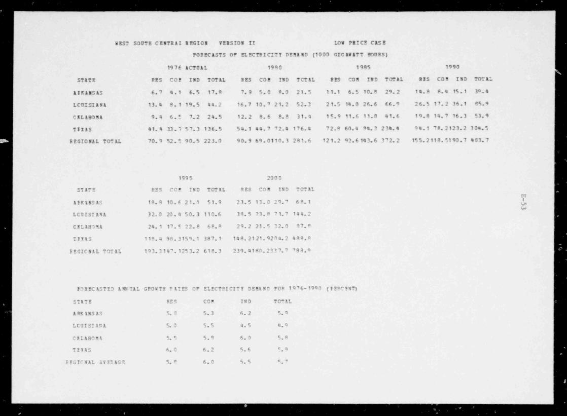
BEST SOUTH CENTR AI R EGION . VERSION II LOW PRICE CASE

FOREC ASTS OF ELECTRICITY DEM A WD (1000 GIG AW ATT BOURS)

1976 A CTU A L 1980 1985 1990

STATE RES COE IND TOTAL RES COR -IND TCTAL R ES C05 IND TOTAL RES COM IND TOTAL

AIKasSAS 6.7 4.1 6. 5 .17.8 7. 9 5.0 9.0 21.5 11.1- 6.5 10.8 29.2 14.8 8. 4 15 . 1 39.4

LCUISIANA 13.4 8.1 19.5 44.2 16.7 10.7 21.2 52.3 21.5 14.0 26.6 66.9 26.5 17.2 36.1 85.9

CELAsoMA 9.4 6.57.2 24.5 12.2 8. 6 8. 8 31.4 15.9 11.6 11.8 41.6 19.8 14.7 16.3 53.9

TIIAS 41.4 33.1 57.3 136.5 54.1 44.7 72.4 176.4 72.8 60.4 94.3 234.4 94.1 78.2123.2 304.5

BEGIONAL TOT AL 70.9 52.5 90.5 223.0 90.9 69.0110.3 281.6 121.2 92.6143.6 372.2 155.2118.5190.7 483.7

1995 2000

STATE RES COE IND TOTAL RES COM IND TOT ALM

AIK15SAS 18.9 10.6 21.1 51.9 23.5 13.0 29.7 68.1 d,w

LCUISI A4 A 32.0 20.4 50.3 110.6 3 9. 5 2 3. R 71. 7 144.2

CFLABOMA 24.1 17.c 22.8 6 8. R 29.2 21.5 32.0 87.P

TFIAS 118.4 98.3159.1 387.1 148.2121.9204.2 498.R

SEGICI AL TOT AL 193.314?.1253.2 618.3 239. 41RO. 23 3 7.7 78 8.4

FOREC ASTED A NN UAL GPOWTH R ATES OF ELECTRICITY DEMA ND FOR 19'6-1990 (t!PCYNT)

STATE RES COM IND TOTAL

A RK 1BS AS 5. 8 5. 3 6. 2 5. 4

LCUISI AN A 5. 0 5. 5 4. 5 4.9

CFIAHOMA 5. 5 5.9 6. 0 5.R

TI1AS 6. 0 6.2 5.6 5. 4

PEGICNAL AVERAGE 5. R 6.0 5. 5 9. 7

|

. .. . - - .-. - .. - - . . . . . - - . . . ~ . . , . . . . _ . . - . . - . . . . . . . - , - -.

'WEST SOUTH CENTR AL REGION VERSION II 10W PRICE CASE

s

FOREC ASTS OF ELECTRICITY PRICE (S / 1000 KWHR)

1976 ACTUAL 19RO 1995 1990

STATE RES CCM IND . TOTAL. RES COM IND TCTAL BES CO M IND TOTAL RES COM IND TOTAL

AIKANSAS 33.9 32.2 22.7 29.3 44.1 41.9 31.2 38.6 57.7 53.4 42.5 50.9 75.7 67.1 54.5 65.5 '

'.CUISI AN A 26.7 27.5 13.3 20.5 35.5 35.0 17.6 27.6 47.8 49.0 24.7 38.0 62.5 62.5 31.3 48.4

C KL AHO M A 29.9 26.2 17.6 25.1 37.7 33.6 24.6 32.0 50.0 45.4 33.1 43.6 64.7 59.0 41.9 55.7

TIIAS 31.2 77.6 18.5 24.8 41.2 36.6 26.9 34.0 57.3 50.0 38.6 47.6 77.4 65.0 52.1 63.6

,

PEGICNAL AVERAGE 30.4 28. 4 18.0 24.9 39.7 36.P 25.1 33.2 53.2 49. 2 34.7 45.0 70.1 63.4 44.9 58.3i

1995 2000

STATE RES COM IND TOTAL RES C05 IND TCTAL

ABKANSAS 95.6 81.5 65.7 80.2 121.1 98.9 77.6 97.3 Y4

LCOISIANA 78. 6 77. C 3 6.3 57.6 9 8. 8 93. e 4 0.2 66.6

CKLAH3MA R1.0 72.5 49.1 67.6 101.8 89.1 55.4 80.5

TIIAS 99.8 80.3 66.8 80.8 128.6 98.4 85.3 102.2'

BEGIC4AL AVE 2 AGE PR.8 77.5 54.5 71.5 112.6 95.0 64.6 86.6i

FO REC ASTED A NN U AL GROWTH R ATES OF ELECTRICITY PRICE FOR 1976-1990 (P E BCE MT)

STATE RES COM IN D TOTAL

45 KANSAS 5. 9 5.4 6. 4 5.9

LCUISIANA 6. 3 6.0 6. 3 6. 3

OKLAHOMA 5. 7 6.0 6. 4 5.9

j TEIAS 6. 7 6.3 7. 7 7.0

B EGIC E AL AYER AGE 6.1 5.9 6. 7 6. 3

- _ - _ - _ _ - _.. _ . . . _ , . -.- _ . . . _ .-- .. .- - . . - .-- . . .

L

WEST SOUTH CENTR AL REGION TERSION II HIG E PRICE CASE

FORECASTS OF ELECTRICITY DER A ND (1000 GIG Av&TT 10095)

1976 ACTUAL 1980 ' 's R 5 1990

STATE RES COF IND TOTAL RES COM IND TOTAL R ES COM IND TOTAL RIS CO M IND TOTAL

AIKANSAS' 6. 7 4.1 6. 5 17.8 7. 0 4.8 8. 0 20.3 7.8 5. 4 10.5 24.4 9.5 5. 8 13.9 30.0

LCUISIANA 13.4 8.1 19.5 44.2 14.7 10.1 19.9 4 e.1 13.7 10.8 22.0 50.0- 14.7 10.9 26.6 56.0

4 CELAHOMA 9. 4 6.5 7.2 24.5 10.4 8.0 8.4 28.4 9.2 8.1 10.0 28.9 9.5 7.6 12.5 31.4

T224S 41.4 33.7 57.3 136.5 48.2 42.0 70.4 165.5 48.1 45.6 P4.3 183.s 55.0 46.3101.8 209.3EEGICNAL TOT AL 70.9 52.5 90.5 223.0 80.4 64.9106.7 262.4 78.8 69.8126.8 286.7 88.7 70.5154.0 326.8

1995 2000

3 STATE RES COE IND TCTAL RES COE IND TCTAL

AIKANSAS 10.0 5.7 17.7 34.4 10.0 5.2 22.2 38.4 g1 iLn '

LCGISIANA 14.8 13.2 33.0 62.3 14.2 9.0 40.7 68.8 'd

j CELAHOMA 9. 7 7. C 15. 6 34.3 9. 5 6.2 19.3 37.1

( T1345 59.6 45.7122.2 234.4 62.3 42.9145.4 259.3 !t

,

REGICWAL TOTAL 94.1 68.6188.4 365.4 96.0 63.4227.5 402.E i

i

FOREC ASTED ANNUAL GROWTH R ATES OF ELECTRICITY DEMANE FOR 1976-1990 ( PERC YNT)'

,

STATE RES COM IND TCTAL I

'ABKANSAS .|. 5 2.5 5. 6 3. 8,

LCDISIANA 0. 7 2.0 2. 7 1. 7;

CRLAH09A 0.1 1.1 4. 0 1. 8

1 TIIAS 2. 0 2.3 4.2 3.1

REGICN AL ATER AGE 1. 6 2.1 3.9 2. 84

I

_ _ _ _ _ _ _ _ _ _ _ _ _ __ _ _ _ _ _ _ _ _ _ . _ _ _ _ _ _ _ _ . _ _ _ _ _ _ _ _ -_

'J EST SOUTH CENTR AI P EGION VERSION II DIG E PPICE C.AS E

FORECASTS OF EL ECTRICITY ?2 ICE (* / 1000 KWHR)

197C ACTUAL 1990 1995 1990

STATE PES C09 IND TOTAL RES COM IND TCTAL B!S COM IMS 70*AL RIS CO M IMD TOTAL

ASKANSAS 33.9 32.2 22.7 29.3 53.1 51.0 40.4 47.5 91.1 89.1 79.2 85.4 127.1124.7115.4 121.0

LCrIISI A7 A 26.7 27.5 13.3 20.5 43.6 44. 4 29.5 37.1 88.7 93.7 75.3 83.0 124.0124.9111.5 117.8

OKLAHOM.% 29. 0 26.2 17.6 25.1 49.6 45.0 36.8 43.2 105.3101.4 94.1 100.0 150.4145.9139.3 144.6

TII4S 31.2 27.6 18.5 24.8 49.6 46.5 38.0 43.7 101.0 99.4 93.0 97.0 144.0139.7140.6 141.3

SECICN4L AVERAGE 30.4 28. 4 1 p. 0 24.9 48.7 46.7 35.9 43.0 96.5 94.9 ' 5. ' 41.4 136.413 3. A126.7 131.2

1995 2000

STATE RES CO2 IND TOTAL R3S COM IND TCTALi

AFKANSAS 2 0 4. 42 02. E 19 3. 4 198.5 335.9334.1324.3 328.8 gg

LCUISIANA 197.8197.~195.9 191.0 3 2 0. 4 319. 53 0 P. 8 312. 9

CELAH01A 237.1232.4225.9 230.7 378.1373.6366.1 370.7

T!X45 225.3220.3227.0 225.2 356.3351.4364.4 360.4

PEGICNAL AV ER A G E 216. 3 213. 320 m.1 211.3 347.7344.7341.0 343.2

FOREC L5?!C A NN UAL GROWTH R ATES OF ELECTRICITY PRICE FOB 1976-1990 (9 ERC!NT)

S141E RES COM IND TCT AL

AFKANSAS 9. 9 10.1 12.3 10. '

LCUISIANA 11.6 11.4 16.4 13.3

CFLAHOMA 12.2 13.0 15.9 13.3

TEIAS 11.6 12.3 15.6 13.2

REGICNAL AVERAGE 11.3 11.7 14.9 12.6

|

(_-- - _ - _ _ _ _ _ - . _ _ _ - .

_ _ _ _ _ _ _ _ _ _ _ _ _ _ _ _ _ _ _ _ _ _ _ _ _ . _

907MTAZN PEGION 7E3SION II PAS T CASE

FOPECASTS OF EL ECTR ICIT Y D25 A ND (1000 GIG AW ATT HOURS)

191 E A CTU AL 1990 1985 1990

STATE RES Cn? IND TOTAL 3ES CDP IN3 TCTAL F ES C09 IND TOTAL BFS CO M IND TOTAL

FC5TANA 2. 2 1. 7 5. 8 9.0 2. 7 2. 4 6. " 12.3 3.7 3.3 8.1 15.4 4.6 4.4 9.0 18. 4

10 ARC 4.1 2.! 5. 5 13.5 5.3 4.4 6. 3 16.4 7.7 5.9 a.1 22.2 10.8 7.7 9.9 29.0

SYOMIN1 1. 0 1.~ 2.1 0.9 1. 5 2. 3 2. 4 6.3 2.3 2. 9 2. 0 9. 2 2.9 3.7 1.5 10.3

"!LCFAD3 5. 4 6.2 4.1 16.8 7. 2 0.0 5. 5 22.1 11.6 10.9 6.7 31.1 17.9 14.5 9.0 43.1

3En PEKICO 2. 0 2.5 2.0 7.5 2. 6 3.5 2. 3 9.1 3.5 4.6 2. 8 11.7 4.5 6. 0 3.4 15.0

hP!20MA 7. 2 6.e 6.1 21.2 1. 4 9.3 E.' 27.4 17.R 13.6 a. 9 42.2 29.S 19.9 11.1 64.1

t!AH 2. 7 2.E 2. 4 8.1 3. 4 3. 2 2. 5 9.P 5.3 4.2 3.3 13.7 9.1 5.5 4.0 18.9

IE7A3A 2. 0 2.! 2.2 7.7 3. 6 3.1 2.2 9.2 6.2 4.' 2.6 14.0 10.1 7. 2 1.1 21.1

FECTONAL TOTAL 27.4 2a.C 30.1 99.6 .16.3 36.1 35.0 112.6 58.1 41." 43.2 159.4 89.9 66.' 52.0 219.7MIuw

1"15 2000

STATE RES COP IN D TOTAL RES COM IN3 TCTAL

F71 TAN 4 5. ' 5.* 10.1 21.9 ?.1 6. P 11.4 25.9

IIAMO 14.5 11. C 12.5 37.9 19.5 12. a 15.8 41.1

E Y O MI NG 3. 6 4.7 4. 2 12.7 4. 4 6.0 *1 15.a

| CCLCEADO 25.9 10. C o.3 57.9 36.3 23. a 10.9 76.9

EEn 3EKICO 5. R 7.7 4.0 18.9 7. 4 9.9 4. 8 23.7

AfI2CNA 45.7 2" . ' 1 3. 9 92.6 69.2 40.3 1 '. 4 132.5

CTAM 11.5 6.5 4.9 24.9 15.8 8.* 6.0 32.7

EEVADA 15.1 10. 7 3. 7 30.5 21.9 15.8 4. 4 43.6

PECICNAL TOTAL 127.7 92. E 6 2. 6 2 4 7.0 193.6125.0 75.9 400.7

|

_

FO B BC ASTIC A NN U AL GROUTH R ATES OF ELECTRICITY DE5AND FOR 1976-1990 ( F ERC EST)

ST&TE RES COM IND TCTAL

PORTANA 5. 3 7.1 3. 2 4.5

IIAHO 7.1 5.8 4. 2 5.6

E YC MI N1 8. 2 5. 5 3. 7 5. 5

- CCICRADO 9. 0 6.2 4. 8 7. 0

BEE MEZICO 5. 9 5. 3 3.8 5.1

AEIZON4 10.7 7.8 4.4 9. 2

CTAH 8. 2 5. 6 3. 9 6. 2

EEVADA 9. 6 7.9 2. 7 7.5

R EGION AL AVFR AGE 8. 8 6.6 4. 0 6.6

TwO)

.

__ _ _ _ _

______ _ _ _ .-

Mo rtN T AIN BEGION VERSICN II BASE CASE

FOREC ASTS OF ELECTRICI'Y PPICE (? / 1000 EWHR)

1976 ACTUAL 1990 1995 1990

STATE RES CO? IND TOTAL RSS COM IND TCTAL PES COM TND TOTAL RIS CO M IND TOTAL

PC9TANA 22.3 20. E 6.1 12.3 25.2 22.9 9. 6 15.9 29.9 23.1 14. ' 21.4 35.7 34.7 20.6 27.4ICAMO 18. 3 17. T 10.2 14.8 22.3 22.1 13.3 18. ' 30.2 29 . 9 1 P. 4 2 5. ' 41.5 39.3 24.3 34.9

hTCMING 24.1 17.7 12.0 16.* 29.9 25.1 10.9 23.9 39.9 36.2 29.4 34.8 52.3 40.3 41.5 47.5C CL 1RA DO 32.6 20.7 19.2 27.6 40.7 37.5 29.2 36.1 53.9 52.' 42.9 50.9 69.0 69.1 59.3 66.9

BEh MEXICO 35.5 27. 7 2 0. P 28.0 41.3 35.3 27.1 14.9 56.0 50.9 4 2. ' 50.4 71.3 67.2 59.6 66.4

ATI2CNA 39. 0 35.2 24.6 33.4 49.8 44.1 35.9 45.5 68.4 69.0 53.0 65.2 43.4 93.9 71.7 89.5UTAM 31.7 26.1 20.0 26.2 37.3 32.4 24.9 32.1 45.9 43.2 35.1 42.2 56.7 55.9 46.9 54.2

EEVADA 28. 4 30 . 4 19.5 26.5 38.3 40.9 25.2 35.9 57.3 60.6 40.5 55.2 92.4 84.2 56.5 79.0

SECIC4 %L AV!R ACE 29.0 25.* 16.6 23.2 35.6 33.0 22.9 30.4 47.7 46. 3 34.6 43.2 62.8 61.7 47.3 58.3

Yu@

1995 2000

STATE RES COP IND TOTAL RES COM IN3 TCTAL

MONTANA 42.7 42.5 27.1 35.3 52.1 52. 5 35.5 44.7

ICAHO 56.2 50.3 30.8 46.0 76.0 64.3 39.0 61.1

nYOMING 66.9 64.7 55.5 62.2 85.8 84.5 73.5 81..

CCLOFADO 89.5 81.8 77.6 87.6 118.3117.0102.9 11' 5

NEW 1EKICO 90 ' 87.E 7E.7 86.6 116.7115.2105.2 1 3.5

APIZONA 127.9125.* 95.2 122.0 176.9167.6126.2 166.9

UTAH 71.2 71.1 61.0 69.0 91.2 40.6 '9.5 9 8. P

EIVADA 114. 6114. E 7 5. 7 109.R 159.4157.1101.2 152.4

RECICMLL AV! PAC?. 82.5 89.F 62.7 77.3 109.7106.1 82.9 103.0

_________ _ _ _ _ _ _ _ - - - - _ _ _ _ _ _ _ _ _ - . _ _ _ __ _ _ _ _ __--_ _ _ _ _ _ _ _ _ _ _ - _ _

_ _ _ _ - _ _ .

FOREC ASTIt ANNUAL GROUTH R ATES OF ELECTRICITY PRICE FOR 1976-1990 (P ERCE NT)

STATE RES COM IND TCTAL

ECNTANA 3. 4 3.8 9.1 6.0

ICAHO 6. 0 S.8 6. 4 E.3

ETCMING 5. 7 7.6 9. 3 7. 8

CCLCRADO 5. 5 6.5 8.2 6. 5

BEE MEZICO 5. 1 6.5 7.7 6. 4

ASIZCNA 6. 4 7.2 7. 9 7. 3

UTAR 4. 2 5.6 6. 2 5. 3

BEVADA 7. 9 7.6 7. 9 9.1

REGIO!AL AT ER AG E 5. 7 6. 5 7. 8 6.8

?.O

--- _ _ _ _

. _ _ _ _ _ _ _ - - _ _ _ _ _ _ . . . _ . . . . .. .

. -- _ _ _ _ - _

97UNTAIN BEGION VERSION II LOU PRIC9 CASE

PORECASTS O' EL ECT9ICIT Y DEM A NC (1001 GIG AW ATT !!O"RS)

19 7 f ACTUAL 1980 1995 1990

STATE PES CDP IND TOTAL RES 00M I?ID TCTAL DES COM IN9 TOT AL RIS COM IND TOTAL

P*NTANL 2. 2 1.~ 5. 8 9.4 2. 7 2.4 6. 4 12.3 1.6 1.9 9.0 15.4 4.' 4.6 9.1 18.4

TIAMO 4. 1 3.' 5.5 13.5 5. 4 4.4 6. 3 16.5 7.9 6.0 0. 0 22.4 11.1 E. 0 10.2 30.0

EYOMING 1. 0 1.7 2.1 4.9 1. 5 2. 3 2. 3 6.3 2.2 1. 0 2. 9 9. 3 3.0 0.0 3.5 10.7

CCLCPADO 5. 4 6.2 4.1 18.9 7. 2 9.3 5.5 22.4 11.' 11.o con 32.3 19.6 If. 4 R.3 46.2

LEE 9EXICO 2. 0 2.? 2. 0 7.5 2. 7 3.7 2.3 9. 4 1.7 5.3 2.9 12. R 5.0 7.2 3.6 17.2

AFI2CNA 7. 2 6.5 6.1 21.2 9. 9 9.5 f.9 2 7. R 17.8 14.4 9.0 43.4 30.9 21.5 11.R 67.6

UI A!I 2. 7 2.f 2. 4 8.1 1. 4 3.2 2. 6 9.8 5.3 4.4 3. 2 11.9 9.2 5.9 4.1 19.4

RTVA3A 2.R 2.5 2. 2 7.7 3. 6 1. 2 2. 3 9.4 6.3 5.1 2.9 14.' 10.6 7. 4 3.5 22.9

T EGICN AL TOT AL 27. 4 29. C 3 0.1 89.6 36.4 37. 1 35.2 114.0 98.4 51.6 41.5 163.1 92.2 75.5 54.0 232.6tnI

@W

1995 2000

STATE FES CO' IND TCTAL RES COM I?!D TCTAL

FONTAN 4 5. 4 6.0 10.5 22.9 7. 5 7.5 12.2 27.9

IC A!!O 15. 5 10. 0 12.9 39.6 21.3 11. 5 16.4 52.1

% Y o MI Nr. 3. 8 5.2 4.4 13.6 4. 7 6.9 5. 4 17.4.

CCLCPADO 27. 7 22. 5 10.0 64.1 19.9 31. 5 12.0 97.9

RE% 1EXICO 6. 7 9.! 4. 5 22.7 9. 9 13.1 5. 6 29."

ABIZONA 49. 2 31 . 4 15.1 101.0 75.7 45.8 14.8 148.a

U T AII 12.0 7.( 5.1 26.4 16.9 9.R 6. 3 35.1

EEVADA If. 3 11. c 4. 3 33.7 2L.4 1?. 0 5. 3 49.2

BEGIONAL TOT 4L 137.1104.E 66.9 324.1 199.1144.T R3.0 446.6

|

i

. . . - - . . . . _ _ _ _ _ _ _ _ . _ _ _ _ _ _ _ _ _ _ _ _ - - . _ _ . _ - . _ . . _ . _

m,_ ___,_

PO B EC ASTIC A NN UAL GROUTH 21T ES 0? EL ECTRI CIT Y DE5kND FCR 1976-1990 (PIRC INT)

STA!! !!S C05 IND TCTAL

PCNTANA 5. 4 7.6 3. 3 4.7

*

ICAHO ?. 4 6.C 4. 4 S. 0

5Y35I50 2. 3 6.1 3. 9 5.7

CCLCFACO 9. 3 7.1 S.1 7. 5

EEE MEZICO 6. 7 6.7 4. 4 f.1

A FI2C5 & 10.9 9.4 4.9 9. 0

UTAH A. 3 6.1 4. 0 6.4

517ALA 10.0 9.7 1. 4 E.1

DESIC5AL 47 ER AF.! 9. 1 7. 3 4. 3 7.1

Y>N

_ _ _ _

_ _ _ _ _ _ _ _ _ _ _ _ _ . _ _ _ _ _ _ _ _ _ _ _ _ _ _ _ ,. . .

_ _ _ _ _ _ _ _ _ _

PCUMTAIN REGICM VFRSION II LO7 PRICS CAS!

F0FFCASTS 7F ELPCTRICITY ?? ICE (S / 1000 Man?)

19 7E ACTUAL 1980 1995 1990

STATE PES COP IND TOT %L PES COM IND TCTAL PES COM TNS TOTAL SIS C0 5 IND TOTAL

FCNTANA 22.3 23.E 6.1 12.1 24.9 22.4 9.1 15.3 2 P.4 26.' 13.2 20.0 32.8 32.1 17.7 25.2

ICAHO 13. 3 17. 5 10.2 14.9 21.9 21.a 12.9 19.2 29.2 21.0 17.1 24.7 40.2 37.9 21.6 33. 1

h YO MI NO 24.1 1'.7 12.0 16.5 29.9 24.3 1a.0 23.1 37.1 3.3.9 26.6 32.3 46.9 45.0 16.0 42.6 |

CCLOPADO 32.6 29.~ 1 c. 2 27.6 39.9 35.7 26.4 34.4 47.7 16. 9 36.6 44.0 5 4.6 59. 9 47.a g7. o

EEE 1EXICO 35.5 27.7 20.0 28.0 39.9 32.0 24.7 32.E 47.2 42.6 24.1 41.9 56.6 54.0 44.3 52.6

AIITCNt 39. 0 35.2 24.6 33.4 47.5 46.3 13.6 43.4 61.4 61.9 46.1 59.9 P 2. 5 9 5. 7 59.R 79.4

{1TAH 31.7 26.1 20.0 26.2 36.2 31.5 23.9 31.1 42.6 41.9 31.9 39.2 51.1 51.9 41.1 49.1

EFTADA 20. 4 31. C 19.5 26.5 15.7 19.8 22.7 13.6 49.0 54 . 4 12.2 4 7. ' 70.2 '5.1 42.7 67.6

REGIC1AL tVE7 AGE 29.0 25. ' 16.6 23.2 34.1 31.' 21.4 29.1 4 2.R 42.3 29.' 39.7 5 4.9 55. 2 3R.9 50.9

tnI

&w

1995 2000

5* LTE P35 CO' IND TCTAL PES CON IND TCTAL

PONTANA 37.0 19.7 22.2 30.7 44.7 46. o 27.7 17.7

ICARO 55.6 47.T 26.2 43.7 ' 3. 6 61.f 31.9 SE.9

5 t O.5I N1 57.3 57.C 45.5 53.4 70.4 72.3 57.0 66.9

CCLOPA00 72.1 74.2 55.3 70.? 91.5 92.5 '?.1 99.2

115 9EXICO 6 f. 4 E.6 . ' 5 4. 5 63.1 ? 9. 9 82.4 67.0 '8.1

AL.20NA 111.1111.2 73.6 105.2 153.9145.1 10.4 142.1

UTAR E 1. 7 64.1 50.9 60.2 76.5 79.6 F2.4 '4.9

EFVADA 99.0101. 1 53.2 93.3 139. 3137.2 66.1 129.9

BEGICN.5 AV ET AG 3 70.0 70. 1 S P. 2 65.1 91.6 89.6 59.5 94.'

* TCT7L INCLUDE 0 TI SC ELL A N EOUS U5!!.

|_ _.. . . . . . . . . . . . . . . _ . . .. _ _ _ _ _ _ _ _ _ . _ _

- -_ _ _ _ - _ _ .

I

70BEC ASTED ANNUAL GROWTH R ATES OF ELECTRICITY PRICE FOB 1976-1990 (PEBCEMT)

SinTE RES COM IND TCTAL

PCBTAN4 2. 8 3.3 7.9 5. 2

ICAHO 5. 8 5. 5 5.5 5.9

EYCMING 4. 9 6.9 R. 2 7. 0

CCLCBADO 4. 3 5.4 6.7 5. 3

EEE 9EXICO 3. 4 4.9 5. 5 0.6

ABIZONA 5. 5 6.6 6. 5 6.4

UTAH 3. 5 5.0 5. 3 4. 6

RETADA 6. 7 6.7 5. 7 E. 9

BEGICNAL AYERAGI 4. 7 5.7 6. 3 5. 9

r.>

,-- - _ - -

. .

- _

._- _ _ _ _ _ _ _ __ _ _ . _ _ _ _ _ _ _ _ _ _ _ - _ - _ _ - - _ - _ _ .

MOUNTAIN REGION TERSIDE II HIGE PRICE CASE

FOREC ASTS OF ELECTRICITY DEM AND (1000 GIG AWATT B00RS)

19 76 A CTU AL 1980 1995 1990

'STATE RES COE IND TOTAL RES COE IND TOTAL B ES COM IND TOTAL RES COM IND TOTAL

PC NTAB A 2. 2 1.7 5. 8 9.9 2. 8 2.4 7.2 12.7 4.1 3.3 8. 9 16.7 5.3 4.3 10.1 20.2

ICAHO 4.1 3.5 5. 5 13.5 5. 5 4.4 6. 5 16.7 8.2 5.9 8. 8 23.4 11.7 7.T 11.0 31.1

BYOMING 1. 0 1.7 2.1 4.9 1. 6 2. 2 2. 4 6.4 2.5 2.9 3.2 8.7 3.3 3.7 3.9 11.1

CCLCBAD3 5. 4 6.3 4.1 16.R 7.4 7. 8 5. 6 22.3 12.5 9.6 7.1 31.2 19.5 12.5 8.4 43.1

AEE MEZICO 2.0 2.5 2.0 7.5 2. 6 3.4 2. 3 9.C 3.5 3.8 2.P 11.0 4.5 4. 7 3.4 13.6

AFIICNA 7. 2 6. 5 ' 6.1 21.2 10.2 9.1 7. 0 27.8 19.3 12.9 0.2 43.5 32.7 18.6 11.8 66.4

UTAH 2. 7 2.f 2. 4 8.1 1. 5 3.1 2.7 10.1 5.9 4.1 3. 6 14.5 9.1 5.3 4.5 20.2

IETADA 2.R 2.5 2.2 7.7 3. 7 3.0 2. 2 9.3 E.6 4.3 2.6 13.9 10.7 6.3 3.1 20.9

IEGICIAL TOT AL 27.4 28.0 30.1 89.6 37.4 35.5 36.0 114.1 62.6 46.7 46.3 162.9 96.8 63.1 56.4 226.7MI-

mAn

1995 2000

SIATE RTS COF IND TOTAL RES CDP IND TCTAL

EONTANA 6.7 5.4 11.6 24.3 8.4 6.7 13.5 29.2

ICAHO 15.9 9.! 14.3 4 C. 9 21.1 12. 8 18.9 53.9

EY0eI41 4. 2 4.( 4.8 13.9 5. 2 5.8 6.0 17.3

CCLOB400 28.0 15 . 5 9. 7 56.8 39.2 18.9 11.? 73.5

EES MEZICO 5. 7 %.! 4. 0 16.4 7. 2 6. 3 4.6 19.6

ABIZONA 49.4 25. f 14.7 94.3 72. 5 34. P 18.1 132.0

UI A!I 13.0 6.5 5.5 26.9 19.1 8.0 6.8 35.2

NFTADA 15.8 9.2 3. 7 29.9 22.8 13.2 4.4 41.9

SEGICNAL TOTAL 138.5 82.3 68.4 303.2 144.5106.5 83.5 403.1

i

70RIC ASTED Ltv DAL CROWTM P 41!3 0F ELECT?ICITY DE5%ND FC? 1976-1000 (?!PCYNT)

S14TE RE S CCM IND *CTAL

PC MT55 % 6. 4 7.1 4.1 5. 2

T C A!!O 7. 7 5.8 S. 0 6. 2

WY11IN~ 9. 2 5.5 4. 6 6.1

CCLCBADO 0. 6 5.1 5. 2 '. 0

6EE MEXICO S. 9 3. 5 3.R 4. 4

AFIZCMA 11.4 7.3 4. 0 8. 5

UTAH 9.1 5.3 4. 7 6.'

EFVADL 10.1 7.0 2. 7 7. 4

R E G IC N AL 1VERAGE 9. 4 6.0 4.6 6.4

MIm@

_ _ _ _ _ _ _ _ _ _ _ .

. . _ _ _ _ _ _ _ _ _ _ _ _

ROUNTAIN REGION TEPSION !! 3!CP ?t!CE CASE

TC2ECASTS 1? ELECTRIC!TY PPIOf (? / 1003 FJH')

1" 7 f ACTUAL 1C#1 to*5 1993

STATE StS CO? IND TOTAL 955 COM IND TCTAL ?!O COM TNS TOTAL 3IS COM IM3 TOTAL

b ?O1TANA 22.3 20.f 6.1 12.3 25.1 23.0 e. ' 15.0 30.1 29.2 15.2 21.6 36.5 34.9 21.2 29.3

ICAHO 18. 3 17.T 10.2 14.9 22.5 22.1 1 ?. 4 18. * 71.6 27. 9 i n. " 26.2 44.5 39.4 24.' 36.2

bYOMING 24. 1 17.7 12.0 16.5 28.9 25.2 19.1 2 4. C 4 C.5 36.5 29.9 35.2 53.9 49.8 42.3 48.4

CCLCBADn 32. C 20.~ 1C.2 27.6 41.9 33.c 29.6 37.5 E 1.9 Ei.6 51.0 59.9 P2.2 R1.3 't.2 79.6

IIs MEXICO 35.5 27.7 20.8 29.0 43.4 37.6 2 c. 3 37.1 69.2 E4.4 55.9 C 3. ' 03.1 97.3 93.5 88.2

III?CsA 39. 0 35.2 24.6 33.4 51.1 49.2 37.2 46.P ?!.3 73.' 59.1 71.2 10 6.213 C. 9 81. 4 100.0

UTA9 21.7 26.1 20.0 2E.2 3'.5 32.7 25.2 32.4 27.9 44. 9 37.1 44.1 60.E 59.3 50.0 57.6

k?1ADA 28. 4 30. 4 19.5 26.5 40.5 42.7 2 ~. 4 37.9 6 P.4 E9.9 50.' 65.1 131.5 96.3 '3.0 95.5

FECICMAL 17??AC? 2'.0 25.! 16.6 23.2 36.5 13.9 23.9 31.3 53.1 57.9 lo.' 4a.2 72.4 69.7 55.5 56.7resImN

1~1S 20 S O

STATE PES CO? IND TOTAL RE3 C3* IMS TCT3L

MONT AN A 44.7 43.C 2A.2 36.2 56.9 53.5 37.2 46.6

ICAHO 61.A 50. 4 31.4 44.1 95.3 64.5 43.1 64.0

n!OMIN7 70.R 66.3 57.7 64.7 93.2 83.0 'F. 0 06.1

CC10PA00 116. 2114. n 13 3. 3 113. 2 166.916'.4149.1 r62.2

ffh MEAICO 133.3129.t121.3 12E.9 19 3. 6190. c l a 2.1 199.'

AFI20NA 155. 1141.7117.3 145.1 226.3193.c168.6 210.1

rIAH 00.5 76.2 68.0 '6.7 10 9. 3130. 3 "2. ~- 103.4

517ADA 148. 313%.7135.0 130.' ?14.5191.2151.2 200.1

REC:(1AL DVEPA0r 101.3 94.~ 79.1 93.9 141.1131.0112.1 132.8

FORIC ASTEE A NNUAL GROWTH R ATES OF ELECTRICITY PRICE FOR 1976-1590 (P EROE NT)

514TE R!S COM IND TCTAL

PCNTANA 3. 6 3.8 9. 3 E.1

ICAHO 6. 6 5.8 6. 5 6. 6

STORING 5. 9 7.7 9.4 8.0

CCLOBADO 6. 8 7.7 9. 9 7. 0

REE MEXICO 7.1 8.7 10.1 E. S

AFI2ONA 7. 4 7.8 9. 9 8.1

DIAR 4. 8 5.9 6. 9 5.8

5EVADA 9. 5 8.6 9. 9 9. 6

R EGIC N AL AYERAGE 6. 7 7. 3 9.0 7.8

aCD

4

_ _ _ . _ _ _,

_ _ _ _

_ _ _ _ _ .

? ACI FTC P E0!CV VEPSICs TI n ASE 27 ICY C?.S *

FOPECASTS OF ELTCTRICITY DEM ASC (1011 GIG AW ATT !! OUTS)

19 7 ( ACTUAL 19A0 1915 19?O

STATE PES CCF IND TOTAL 7ES COM IMD TCTAL FES C09 IND 77TAL RIS COM IMD TOT AL

BASHIN1!ON 22.3 10.7 29.0 62.4 26.8 13.2 20.9 72.1 ?2.1 1'. 4 2 a. 6 96.7 37.3 22.3 40.4 103.1

C511CN 12.4 7.5 13.6 34.3 13.9 10.5 15.0 41.1 16.6 18.6 19.5 55.2 19.8 20.1 23.9 74.4

CAIIf75NIA 45.1 49. C 4 9. R 150.4 53.9 62.5 4P.1 173.0 5 9.3 e3. 6 SE.9 214.1 68.9112.7 69.2 268.6

TIG!rNAL TOTAL 79.4 69. 2 R A. 4 240.5 71.6 R6. 8 9 3. 0 296.2 10 a.0111. 6111. 0 356. 0 125.5175.1133.4 446.1

<

1935 2000

STATE PES CCP TMD TCTAL 7ES C1? IND TCT4L

nASHIN1 TON 42.5 29.2 47.2 121.5 45.1 35.4 55.3 143.0 me

CRIGCN 2?. 2 46. E 2 9. i 100.1 2 7. 0 'r2. 2 3 5. 6 136.* $$

CALIfCBNT4 77. 41'45.4 9 ?. 6 32a.6 95. 9185.8100.7 396."

BEGIONAL TCTAL 1'43. 5220. 4159: 9 550.2 161.0293.ctn1.6 672.1

FOREC ASTFD A 45UAL GPOWTH P ATES OF ELECTFICITY PRICE FO? 1" 6-1999 (" F SC' NT),

S14TE RES CCM IND TCTAL

%ASHINGT04 6. 5 7.9 11.2 F. 6

CRF10N 5. 1 9.6 9. 6 9. 5

C41If0FNIA 6. 5 7.5 4.5 7. 5

PIGICNAL .A7ERAGE 6.1 8.2 9.9 7.9

PACI FIC REGION TERSION II B ASE P3 ICE CASE

FOREC ASTS OF ELECTRICITi PRICE ($ / 1000 K3HE)

197 f ACTUAL 1980 1995 1990

STATR RES CCE IND TOTAL RES COM IND TCTAL BES COM IND TOT AL RIS CD P IND TOT AL

WAERINGTON 12.7 14.1 4.5 9.1 17.2 20.1 R. 4 14.0 23.5 28.9 13.8 20.6 30.0 41.1 20.0 29.7

CBIGCN 18.6 1'.2 2. 0 14.0 22.7 27.5 11.9 10.5 29.2 36.6 19.0 27.7 37.3 62.3 25.4 43.7

CAIITORNIA 35.4 33.4 24.3 31.1 46.6 46.2 35.5 43.1 67.4 69.5 57.4 65.4 85.5 91.5 76.5 95.7

BEGICIAL ATERAGE 22. 2 21. E 12. 3 16.1 29.9 29.7 19.6 25.2 40.0 45.0 29.7 ? 7. 9 51.2 63.9 40.6 92.7

1995 2000

STATE DES CC? IND TCTLL RES COM I10 TCT3L

EASHINGTON 38.6 57. C 2 6. 9 38.3 4 R. 4 79.7 35.7 51.3 mI

CRIGON 46.3105.2 37.8 70.5 57.7181.1 44.5 12C.3 gj

CAIIPORNIA 119. 4130. f 111. 4 122.6 169.6187.'161.6 1'6.2

BECICN4L A V E3.t G E 68.1 97.7 57.3 77.1 91. 6149. 5 R 3. 6 115.9

POREC LSTED A 1"ULL GPO'dTH P 41?S OF ELECTRICI2 Y DB5A N D PCL 1" 76- 19"O ( E EPC F77)

STLIE RES CCM I9D TCT AL

LA!H14GT04 3. 7 5. 4 2. 4 3.5

CRIGON 3. 4 10.1 4.1 5.7

CAII!11"'' 3.1 6.C 3.0 4. 2

P EGIC N AL AVEP AGE 3. 3 6.5 1. 0 4.3

-_ _ _ _

i

JwarI't

LA 4 1 7 0T .

O 5 5 9 0T 7 7 9 7

1 2 4

_D 1 2 4A.

.

.

0 I 1 4 1 69 4 2 7 1

9 11 M 9 6 9 2

O . .

C 2 0 2 62 3 2 7

1 1

4 01 -Sf . .

3 8 0 5 4_ 3 2 ' 3_

_ 1

L9 0 9t. 9

T .

O 7 5 6 9T A 5 2 6)

S 2 3?" D ?0 '. 90 N .

9 5 I 5 o o 33 3 t S 1

T 9 1

T 1 9 7 * 1 6T)

% n . ." 7 O 7 9 1 6 M0 1 1 1 c 2 7

\ " 1 "1 R6 9 '.C I 3

5" F .

T F 2 6 2 2 T(

_ C 1 3 1 6 1_

I 9 1

9 1'P 1 0

L L 9(

1 \ C 15 1 8 5 i. 4E 1

. T . -C O TI X C 2 1 6 9 C 3 9 1 9 t

3 6 '4 7A T ' 4 ' 1 T1'4 1 4 ' 0

E'1 2

1 L9 * A F: 9 9 'S 7 1

1- 0 5 5 ". 6 2

R T . . .. 9 .

Y 0 I 0 0 a 4 1 1 6 6 7 C O C 3 9 c. 4T 9 3 1 4 9 $ 5 3 0 0 T TI 9 2 1 2

2 R 4 2 6 2 CC 1 ? 4 0 2 6N3 . . . .I o .

R C 1 1 4 9 C 6 3 3 4 t

T 1 1 6 9 3 7 1 2 92 2 3 ST 5 9 0 6 5 S 9 7 5 1 D D 5 2 2 2

L " . . . . 9 . . . . N . . . .

T 3 6 1 1 2 7 1 9 4 4 Y I 2 4 1 3

2 1 5 1 5 2 0 9 T' 1 1 !O c

I

O L L RA 1 1 T1 3 4 5 2 6T \T . . C_

_ S T

.

5 2 7 0_

I A O 3 4 0 9 O 5 2 5 3 ' 5_

.

I C T 6 3 5 4 T 2 0 6 1 L 0_

_

E L 1 2 1 1 3 5 E C S 0 6 7.

1_

N P g_

9 D 5 T_ O O U D 0 6 4 2 9 6

O_ I F T N N .",. 9 ". I 5 a 7 %3 O I 9 2P L 2 1 4 9 " 4 2 3 6 ".' 7 1 E

T f 2 1 M T F 5 ( I77 t '. . . T . . . . % S 9 6 7 s' O

__ * C " ' "4

C 9 7 4 9 P ? . . . .91 1 6 2 4 6 4 3 3 3 3 3_

N 1 2 HO 3 3 4 1 9 S 1 1 1 6 TI 2 . . . . E . . . . WG C 2 2 5 9 D 4 4 9 ' 0? 2 1 4 7 4 2 r. 5 F.

1 rP

" LI 1

? U!T T eC

T t L A ciE t A

T ' O nO 7 * eT ~ T v

S s- N A L K i L A N 7

- E O ! t E O r A C O I tT T M 5 5 T T 5 g M E E T M M 4A G C 9 C L C 0 f C 3 T G C 9 5

T M C n I " 1 1 a I 0 \ 1 G 0 cI Y 7 C 7 t 1 E F IS 1 F Y G !l 5 I E S 9 S I a9 R I R

! C I F Ei C I F S C I et. A A t A A RS C % c % C

-

|I || |||

- _ _ _ _ _ _ _ _ _ _ _ . . _ _ _ _ _ _ _ _ _ _ _ _ _

P ACI FIC REGION VERSION II 109 PRICE CASE

POPECASTS OF EL ECTRICIT Y P7IC E ($ / 1000 KWRP)

197E ACTUAL 1980 1995 1990

STATE PES COM IND TOT 4L RES COM IND TCTRL RES COM IND TOTAL LIS COM IND TOTAL

WASHINGION 12.7 14.1 4.5 9.1 16.7 19.6 7.9 13.5 22.0 2'. 6 12.1 19.1 28.0 38.6 16.7 25.8

CREGCN 18.6 17. 2 P. 0 14.0 22.1 22.3 11.1 17.9 27.4 35.1 16.0 26.0 33.6 59.6 21.4 40.2

CALIF 0RNIA 35. 4 33.4 24.3 31.1 42.6 42.2 31.5 39.1 53.0 55.6 43.0 51.3 64.5 72.1 55.6 65.6

BEGICMAI Av!OAGE 22.2 21.E 12.3 16.1 27.1 29.0 16.9 23.5 34.1 39.4 2 3. ' 32.1 42.0 56.9 31.2 43.9

1995 2000

STATE RES COM IND TOTAL 9ES CDP IND TCT4L

EASHINGTON 33.9 53.1 21.2 33.4 41.0 73.7 26.8 43.6ts1

CRECCN 39. 9101. C 2 6. R 64.7 47.6174.4 33.4 110.9 daha

CAIIPORNI% 76.1 41.( 60.3 81.6 90.3119.3 A3.7 102.9

BECIC'f4L AV E 9713 50.0 81.T 3 A. 8 59.9 59.6122.1 4 7. " 95.A .

F7 BEC ASTF 7 '5^ ITAL GROWTH PPTF3 OT EL ECTRICIT Y PRICE FOP 1976-1990 ( P FBCE NT)

S 'I ti t RE S COM ND TCTAL

W A f 4 T nGIO , 5. 8 7.5 9. 8 7.7

f S FGC N 4. 3 9.2 7. 3 7. 9

CAIIf0ENIA 4. 4 5.7 6.1 5. 5

REGIcNAL AVEC4GE 4. 7 7.2 6. 9 C. 5

. _ _ _ - _ _..

- - - - - ~--

PSCIFIT ??GION VERSYON II HIG P PRIC2 CAS2

FOR EC ASTS O' EL ECTRICITY DE5&ND (1003 GIc 4W ATT "OURS)

19 7 ( LCTUAL 1990 1995 1990

STATE TES COR IND TOTAL 39S CO* IND TCTAL RES C09 IND TOTAL RES CO 3 IND TOTAL

E 4 5 9 IN 3TO N 22. 1 13.7 29.0 63.9 26.8 11.3 29.9 72.1 32.0 17.3 34.5 A6.3 36.9 22.1 40. 1 102.2

CFIGCN 12. '.T 13.6 34.3 13.9 10. c 15.9 41.1 I f.5 19.5 19.5 55.0 19.6 29.9 23.7 73.9CA LIFORNI A 45.1 49.6 45.R 150.4 30.2 60.e 47.' 169.9 55.7 76.6 59.4 201.0 62.1101.6 66.8 246.9

F E CION A L TOT AL 79. R 69.2 89.4 24R.5 90.8 85. C 9 3. 4 233.c 104.2112.4109.3 342.4 118.6153.6130.7 423 0

1

1995 2000

STATE RES COM IND TOT 4L RES COM IND TCTAL

E n f HIN GIO N 41. R 2'. 5 4 6. 8 120.0 47.0 35.0 54.8 140.97CREGON 22. 9 46.5 29.9 99.1 26.3 71.7 35.2 134.5 [j

CAIIfcENIA 66.6124.C 79.5 289.3 68.6149.5 93.9 333.1

PECIONAL TOTAL 131.2199.315'.2 508.5 141. 92 55. 21 R 3. R 608.9

FOREC ASTED A NN U AL GROWTH P ATES OF ELECTRICIT Y DEMANE PCR 1976-1990 ( T ERC YNT)

STATE 9ES COM IND TOTAL

E Af RINGTO N 3. 7 5. 3 2. 4 3.4

CRIGON 3. 3 10.0 4.0 5. 6|

i CAIITOENIA 2. 3 5.3 2. 7 3.6

R EGICN AL AVE 0 AGE 9 6.0 2. 8 3. 9

_ _ _ _ _ _ _ _ _ . - ____ _ _ _ _ _ _ _ _ _ _ _ _

HIG E PRICE CASE ,

PACIFIC REGION TERSION II

FOPECASTS OF ELECTRICITY PRICE ($ / 1500 NUBR)

19 7 6 A CTU AL 1980 1985 1990

STATE RES COM IND TOTAL RES C05 IND TCTAL RES COM IND TOTAL RIS CO R IND TOTAL

N A SHIN GTO N 12.7 14. 1 4.5 9.1 17.2 *0.1 8. 5 14.1 24.0 29.4 14.4 21.2 32142.221.5 30.0

CEIGCN 18. 6 17. 2 8.0 14.0 22.8 23.0 11.9 18.6 29.7 27. 0 18.5 28.2 38.9 63.4 27.1 45.1

CAIIFORNIA 35.4 33.4 2a.3 31.1 51.3 50.8 40.1 47.7 89.3 90.8 79.1 86.9 117.8122.3108.5 117.1

REGICMLL AVERAGE 22.2 01.E 12.3 18.1 30.4 31.3 20.2 26.8 47.7 52.4 37.3 45.4 62.9 76.0 52.4 64.1

-

1995 2000

EIATE RES CCF IND TOTAL RES COE IND TCTAL

NASHINGTON 4 0. 7 58. E 2 9. 4 40.5 51.8 82.5 39.6 54.8

YCREGON 49.2107.3 36.9 73.1 62.7184.4 49.9 124.0 2

CAIIf0fMIA 200.3208.2191.9 201.4 345.5357.2338.0 348.8

PECICN AL AV ER AGE 96. 7124. E 86.1 105.0 153.3208.0142.5 176.1

e

t

I

F0DEC ASTEC A N104L GROWTH P AIES OF ELECTRICITY PRICE FOR 1976-1990 (P E RCE NT))

STATE RES CO.9 IND TOTAL

E A !HIN F.TO N 6. 8 8.2 11.8 8.9

CffCCN 5. 4 S.8 9.1 P. '

CAIIYCENIA 9. 0 9.7 11.3 9.9

REGICMAL AVERAGE 7. 7 9.4 10.9 9.5

- - _ - _ _ _ _ _ _ _ _ -_-

NUREG/CR-1295GRNL/NUREG-63

Dist. Category RE

INTERNAL DISTRIBUTION

1. M. Baker 21. W. R. Mixon2. R. S. Carls: :n 22. S. C. Parikh3. H. S. Chang 23. A. M. Perry|

! 4-8. W. S. Chern 24. R. M. RushL 9. S. M. Cohn 25. R. C. Tepel

10. R. M. Davis 26. J. L. Trimble11. J. W. Dick 27. T. J. Wilbanks12. W. Fulkerson 28. D. J. Wilkes13. C. A. Gallagher 29-30. Central Research Library14. D. L. Greene 31. Document Reference Section15. E. A. Hirst 32. Laboratory Records (RC) l16. R. B. Honea 33-34. Laboratory Records |17. C. R. Kerley 35. ORNL Patent Office '

18. H. M. Long 36. Nuclear Safety Information19. R. J. Maddigan Office20. J. B. Mills 37-149. Economic Analysis Section

EXTERNAL DISTRIBUTION<

150. Institute of Energy Analysis, ORAU Library, Oak Ridge, TN 37830151-152. Technical Information Center, DOE-0RO, Building 1916T-1,

Oak Ridge, TN 37830153. Assistant Manager, Office of Research and Development, DOE,

P. O. Box E, Oak Ridge, TN 37830154-301. Energy Demand Analysis Group Distribution List, Economic Analysis

Section, Energy Division302-566. Distribution Category RE (NTIS 10)

|

|

|

|

:|

e U S. GO'dRNMENT PRINTING OFFICE: 1984 640 245/161

I

"ORNL State Level Electricity Demand Forecasting Model." - Nuclear ...

Documents

Transcript of "ORNL State Level Electricity Demand Forecasting Model." - Nuclear ...