Applied Energy 87 (2010) 3584–3590

Contents lists available at ScienceDirect

Applied Energy

journal homepage: www.elsevier .com/ locate/apenergy

Analysis and forecasting of nonresidential electricity consumption in Romania

Vincenzo Bianco a, Oronzio Manca a,*, Sergio Nardini a, Alina A. Minea b

a Dipartimento di Ingegneria Aerospaziale e Meccanica, Seconda Università degli Studi di Napoli, Via Roma 29, 81031 Aversa (CE), Italyb Faculty of Materials Science and Engineering, Technical University Gh. Asachi from Iasi, Bd. D. Mangeron, No. 59, Iasi, Romania

a r t i c l e i n f o a b s t r a c t

Article history:Received 1 January 2010Received in revised form 1 May 2010Accepted 17 May 2010Available online 14 June 2010

Keywords:Electricity consumptionForecastingElasticityGrey modelRomania

0306-2619/$ - see front matter � 2010 Elsevier Ltd. Adoi:10.1016/j.apenergy.2010.05.018

* Corresponding author. Tel.: +39 081 5010 217; faE-mail address: oronzio.manca@unina2.it (O. Man

Electricity consumption forecast has fundamental importance in the energy planning of a country. In thispaper, we present an analysis and two forecast models for nonresidential electricity consumption inRomania. A first part of the paper is dedicated to the estimation of GDP and price elasticities of consump-tion. Nonresidential short run GDP and price elasticities are found to be approximately 0.136 and�0.0752, respectively, whereas long run GDP and price elasticities are equal to 0.496 and �0.274 respec-tively.

The second part of the study is dedicated to the forecasting of nonresidential electricity consumptionup to year 2020. A Holt–Winters exponential smoothing method and a trigonometric grey model withrolling mechanism (TGMRM) are employed for the consumption prediction. The two models lead to sim-ilar results, with an average deviation less than 5%. This deviation is to be considered acceptable in rela-tion to the time horizon considered in the present study.

� 2010 Elsevier Ltd. All rights reserved.

1. Introduction

Electricity consumption has become a topic of immense impor-tance. The growing interest in the area has largely been triggeredby the growing demand for energy across the world fuelled mainlyby increasing economic activities, particularly in the emergingcountries.

It is important to understand and be able to predict electricityconsumption in order to effectively manage its generation and sup-ply. Estimating electricity consumption in advance is crucial inplanning, analysis and operation of power systems in order to en-sure an uninterrupted, reliable, secure and economic supply ofelectricity.

Electricity consumption forecasting ranks amongst the mostimportant issues in today’s developed and developing countries,because it allows for a correct programming of investments inthe electric sector. This is a nodal point, because for many years,with the raise in living standards and the development of industry,the demand for electricity has been increasing.

The aim of the present paper is to analyze and forecast nonres-idential electricity consumption in Romania utilizing differenttechniques.

To the best of authors’ knowledge, this is the first attempt tostudy in detail, nonresidential electricity consumption in Romania.In fact, open scientific literature dealing with this topic is extre-mely scarce.

ll rights reserved.

x: +39 081 5010 204.ca).

The first objective of the present paper is to analyze electricityconsumption, estimating the consumption equation by means ofthe usual econometric techniques. Therefore, it is possible tounderstand the consumption drivers and estimate the elasticities.

The second target is to propose an accurate and simple forecast-ing model for nonresidential electricity consumption. To thisscope, because of the short historical series and complex patternof the electricity consumption, a grey prediction model and aHolt–Winters exponential smoothing technique are used to buildtwo models, in order to forecast electricity consumption up to year2020. Particularly, a grey model is employed due to its ability topredict the future values of a time series by using few data pointsand because of its computational efficiency [1].

The performances of the two models are compared and dis-cussed, showing a good accord.

The information contained in the present paper is believed to beuseful for energy planners and managers. In fact, the knowledge ofprice and income elasticities allows electricity companies to designconvenient demand policies and helps policy makers to formulatepolicies to reform the electricity sector. Whereas, the demand fore-cast is important for potential investors in the electricity sector andfor the companies involved in the electricity business which needto plan their future strategies.

2. Literature review

In the last 15 years, because of the increase of living standardsand the fast growth of developing countries a strong increase of

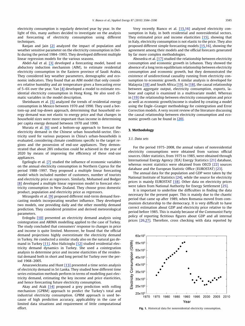
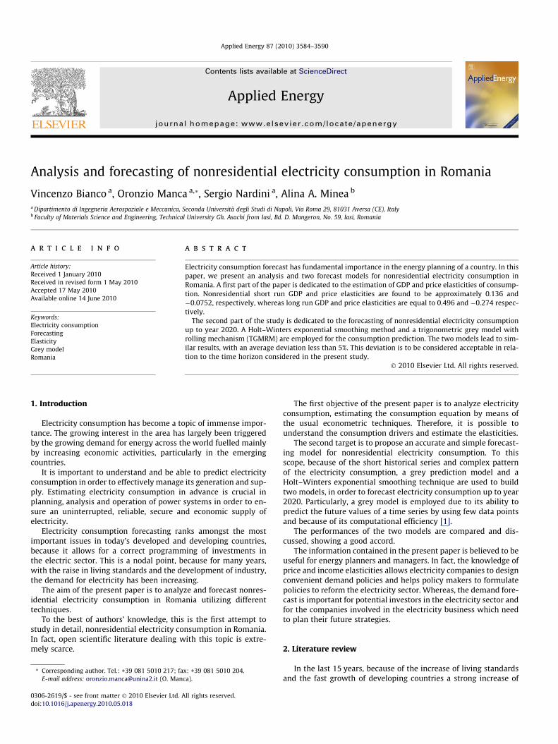
Fig. 1. Historical data for nonresidential electricity consumption.

V. Bianco et al. / Applied Energy 87 (2010) 3584–3590 3585

electricity consumption is regularly detected year by year. In thelight of this, many authors decided to investigate on the analysisand forecasting of electricity consumption using differenttechniques.

Ranjan and Jain [2] analyzed the impact of population andweather sensitive parameter on the electricity consumption in Del-hi during the period 1984–1993. They developed different multiplelinear regression models for the various seasons.

Abdel-Aal et al. [3] developed a forecasting model, based onabductory induction mechanism (AIM), to estimate residentialelectricity consumption in the Eastern province of Saudi Arabia.They considered key weather parameters, demographic and eco-nomic indicators. They found that an AIM model that only consid-ers relative humidity and air temperature gives a forecasting errorof 5–6% over the year. Yan [4] developed a model to estimate res-idential electricity consumption in Hong Kong. He also used cli-matic variables in the model description.

Sheinbaum et al. [5] analyzed the trends of residential energyconsumption in Mexico between 1970 and 1990. They used a bot-tom-up and top-down approach, determining that household en-ergy demand was not elastic to energy price and that changes inhousehold sizes were more important than income in determiningper capita energy demand between 1970 and 1990.

Murata et al. [6] used a bottom-up approach to forecast theelectricity demand in the Chinese urban household-sector. Elec-tricity used for various purposes in China’s urban-households isevaluated, considering climate conditions specific to the target re-gions and the possession of end-use appliances. They demon-strated that about 28% reduction could be achieved in the year of2020 by means of improving the efficiency of these end-useappliances.

Egelioglu et al. [7] studied the influence of economic variableson the annual electricity consumption in Northern Cyprus for theperiod 1988–1997. They proposed a multiple linear forecastingmodel which included number of customers, number of touristsand electricity price as regressors. Similarly, Mohamed and Bodger[8] developed a multiple linear regression model to forecast elec-tricity consumption in New Zealand. They choose gross domesticproduct, population and electricity price as regressors.

Mirasgedis et al. [9] proposed different mid-term demand fore-casting models incorporating weather influence. They developedtwo models, one providing daily and the other monthly demandprediction. They considered primitive and derived meteorologicalparameters.

Erdogdu [10] presented an electricity demand analysis usingcointegration and ARIMA modelling applied to the case of Turkey.The study concluded that consumers’ response to changes in priceand income is quite limited. Moreover, he found that the officialdemand projections highly overestimate the electricity demandin Turkey. He conducted a similar study also on the natural gas de-mand in Turkey [11]. Also Halicioglu [12] studied residential elec-tricity demand dynamics in Turkey. She used a cointegrationanalysis to determine price and income elasticities of the residen-tial demand both in short and long period for Turkey over the per-iod 1968–2005.

Amarawickrama and Hunt [13] presented a time series analysisof electricity demand in Sri Lanka. They studied how different timeseries estimation methods perform in terms of modelling past elec-tricity demand, estimating the key income and price elasticities,and hence forecasting future electricity consumption.

Akay and Atak [14] proposed a grey prediction with rollingmechanism (GPRM) approach to predict the Turkey’s total andindustrial electricity consumption. GPRM approach is used be-cause of high prediction accuracy, applicability in the case oflimited data situations and requirement of little computationaleffort.

Very recently Bianco et al. [15,16] analyzed electricity con-sumption in Italy, in both residential and nonresidential sectors.They estimated price and income elasticities [15], showing thatin Italy, electricity consumption is not elastic to the price. They alsoproposed different simple forecasting models [15,16], showing theagreement among their models and the official forecasts generatedby far more complex methodologies.

Abosedra et al. [17] studied the relationship between electricityconsumption and economic growth in Lebanon. They showed theabsence of a long term equilibrium relationship between electricityconsumption and economic growth, but they demonstrated theexistence of unidirectional causality running from electricity con-sumption to economic growth. A similar analysis is developed forMalaysia [18] and South Africa [19]. In [18], the causal relationshipbetween aggregate output, electricity consumption, exports, la-bour and capital is examined in a multivariate model. Whereasin [19] the relationship between electricity consumption and priceas well as economic growth/income is studied by creating a modelusing the Engle–Granger methodology for cointegration and ErrorCorrection models. A very recent review of the literature discussingthe causal relationship between electricity consumption and eco-nomic growth can be found in [20].

3. Methodology

3.1. Data sets

For the period 1975–2008, the annual values of nonresidentialelectricity consumptions were obtained from various officialsources. Older statistics, from 1975 to 1985, were obtained throughInternational Energy Agency (IEA) Energy Statistics [21] database,whereas recent statistics were obtained from OECD [22] sourcesdatabase and the European Statistic Office (EUROSTAT) [23].

The annual data for the population and GDP were taken by theNational Institute of Statistics [24], while the source for electricityprices is mainly EUROSTAT [18]. Other data on electricity priceswere taken from National Authority for Energy Settlement [25].

It is important to underline the difficulties in finding the datanecessary for the present paper. This is mainly due to the chaoticperiod that came up after 1989, when Romania moved from com-munism dictatorship to the democracy. It is very difficult to havecorrect estimation about GDP and electricity price relative to theperiod before 1985. This is mainly because of the Communist Partypolicy of reporting fictitious figures about GDP and all internalprices [26,27]. Therefore, cross checking with data reported by

3586 V. Bianco et al. / Applied Energy 87 (2010) 3584–3590

international organization (i.e. IEA and EU) was necessary to vali-date the data.

In Figs. 1, 2a and b, electricity consumption, GDP and electricityprice are reported respectively. A substantial linear growth trend innonresidential electricity consumption during the period 1975–1989 is observed. Whereas in 1990, a marked decrease of nonres-idential electricity consumption was detected. This is mainly be-cause of the Romanian Revolution that had a strong effect inindustrial life. Between 1989 and 1994 the industrial sectorcrashed down, especially the heavy one (metallurgical industry).After 1994 the industrial sector stabilized with low increases anddecreases depending on market conditions. However, after the year2000, a substantial growth trend in the electricity consumption canbe observed.

As for GDP, Fig. 2a, a slight increase during the year 1985–1988and a strong decrease from 1989 up to 1992, reflecting the situa-tion of political instability inside the country can be detected. After1992, there is a period of stabilization up to the year 2000, withslight increase of GDP. From the year 2000, a strong increase inGDP can be observed, highlighting Romania as one of the mostattractive emerging countries. This is mainly due to foreign invest-ments, especially from Western Europe, in industrial activitiesthanks to the lower cost and good quality of labour and to the riseof the service sector (i.e. financial, IT, etc.), which has a high valueadded.

Nonresidential electricity price, Fig. 2b, shows a substantial in-crease for all the considered period, 1975 up to 2007. This behav-iour is mainly due to the increase in the prices of coal and gas,which represent the main primary energy sources used in Romaniato generate electricity. The marked growing trend observed from2005 up to 2007 clearly reflects the record prices reached by oil,coal and gas on the financial markets during this period.

3.2. Elasticities estimation

In this section, a single equation demand model for nonresiden-tial electricity consumption in Romania is presented.

The consumption equation is expressed in linear logarithmicform, linking electricity consumption to GDP and price. The equa-tion takes the classical form of a standard dynamic constant elas-ticity function of consumption [10,15,28,29]:

logðYnon res;tÞ ¼ a0 þ a1 logðPRnon res;tÞ þ a2 logðGDPtÞþ a3 logðYnon res;t�1Þ ð1Þ

where Ynon_res,t is the nonresidential electricity consumption,PRnon_res,t is the electricity price, GDP is the gross domestic productand ai are the regression coefficients, whereas the subscript t � i

Fig. 2. Historical data for the explaining vari

indicates the lag term. Data from 1975 to 2007 are utilized to esti-mate Eq. (1).

The coefficients a1 and a2 are of fundamental importance, be-cause they represent the short running price and GDP elasticitiesof nonresidential electricity consumption.

As for the expected coefficients signs in Eq. (1), one expects thata2 is greater than zero, because higher GDP should result in greatereconomic activity and accelerate purchase of electrical goods andservices [12]. On the contrary, price elasticity (i.e. a1) is expectedto be less than zero in accordance with the usual economic reason[10,28].

According to the partial adjustment model specified in Eq. (1),from the short run elasticities, it is possible to calculate the longrun elasticities by dividing a1 and a2 by (1 � a3) [10,11,15,28,30]:

E PR ¼ a1=ð1� a3ÞE GDP ¼ a2=ð1� a3Þ

where E_PR and E_GDP are the long run price and GDP elasticities ofnonresidential electricity consumption.

The results of these estimates for nonresidential electricity con-sumption are reported in Table 1.

The Augmented Dickey Fuller (ADF) test is used to test for thepresence of unit roots and establish the order of integration ofthe variables (i.e. the natural logarithm of Ynon_res,t, PRnon_res,t andGDPt) in the model. On the basis of ADF statistics, reported in Table2, the null hypothesis of a unit root cannot be rejected at 5% level ofsignificance for the series Ynon_res,t and GDPt. Stationarity is ob-tained by running the ADF test on the first difference of the vari-ables, indicating that the series Ynon_res,t and GDPt are integratedof order 1, I(1) in nature. Therefore, Eq. (1) is valid only in the spe-cific period of time considered (i.e. 1975–2007) and it cannot beused to forecast future demand [30].

There is the possibility that the ordinary least square (OLS) re-sults may be misleading due to inappropriate standard errors be-cause of the presence of heteroskedasticity [10,11]. Therefore, totest for the presence of heteroskedasticity, White heteroskedastic-ity test (without cross terms) is performed. Since White’s test sta-tistic value of 5.97 is smaller than 95% critical v2 value of 12.59, itis possible to confirm the null hypothesis of no heteroskedasticity.

To account for the presence of serial correlation, the Breusch–Godfrey Serial Correlation LM test is applied to the model. SinceBreusch–Godfrey’s test statistic value of 1.79 is smaller than the95% critical v2 value of 3.84, it is possible to confirm the nullhypothesis of no serial correlation in the residuals.

Another source of error for Eq. (1) can be represented by ‘‘mul-ticollinearity”. Observing the value of R2 and t values reported inTable 1, it can be concluded that multicollinearity is not present.

ables considered: (a) GDP and (b) price.

Table 1Summary of statistics, coefficients and estimation of price elasticities over the period1975–2007 for Eq. (1) (the t statistics are reported in parenthesis).

Eq. (1)

a0 2.060 (3.809)a1 �0.0752 (�5.390)a2 0.136 (5.283)a3 0.726 (12.610)E_PR �0.274E_GDP 0.496R2 adjusted 0.954F 217

Table 2Augmented Dickey Fuller (ADF) unit root test on the logarithms of the consideredvariables. The confidence level, at which the hypothesis that the series contains a unitroot can be rejected, is reported in parenthesis.

Variables ADF test statistic Test equation

Ynon_res,t �2.506 (67.6%) Constant + trendGDPt �0.432 (10.9%) ConstantPRnon_res,t �5.160 (99.9%) None

First differenceYnon_res,t �2.880 (99.5%) NoneGDPt �2.484 (98.5%) None

V. Bianco et al. / Applied Energy 87 (2010) 3584–3590 3587

In fact, given a high value of R2, the t values indicate that all thecoefficients are statistically different from zero at a very high de-gree of confidence (greater than 99%) [30]. This also confirms thatthe number of observations used to estimate Eq. (1) was appropri-ate [30,31].

As shown by the diagnostic tests performed on the residualsand by the statistics reported in Table 1, Eq. (1) can be considereda valid relationship to describe nonresidential electricity consump-tion in Romania from 1975 to 2007.

3.3. Grey prediction model

In the light of the findings of the previous section, a classicaleconometric model, such as the ones presented in [12,15,28] can-not be used, because GDP and price are not to be considered asexplaining variables, as demonstrated by their low elasticities[10,15]. Therefore, it seems better not to include them in the fore-casting model and ‘‘let the consumption data speak for itself”. Thepresent case shows an anomalous consumption pattern, due topolitical instabilities of 1989, which provoked a strong decreasein electricity consumption and a deep change of the economic sys-tem. To build a reasonable model the data before 1989 are notused, resulting in a relatively short series of the historical data.

Due to the aforementioned reasons, Romania’s energy demandstructure can be characterized as unstable and complex. Given thisanomalous electricity consumption pattern, the grey forecastingmodel represents an effective tool to build a reliable forecasting.This method is characterized by a low amount of input data andhigher forecasting accuracy when compared with other forecastingtechniques.

For these reasons, the grey forecasting model [32] is employedto predict the future consumption of nonresidential electricity inRomania. This kind of model gained their popularity in time seriesforecasting due to their simplicity and ability to characterize anunknown system by using few data [14,33]. Besides, it is morepracticable and user friendly when compared to Box–Jenkins mod-els and artificial intelligence techniques which require more effortand time for parameters identification and model building phase[14].

Among the family of grey forecasting models, the GM(1, 1)model is the most frequently used because it ensures a good com-promise between simplicity and accuracy of the results. TheGM(1, 1) model begins by converting the original data series intoa monotonically increasing data series by a preliminary transfor-mation called accumulated generating operation (AGO). Applyingthe AGO technique will cause an exponential pattern and, hence,a reduction of the noise in the original data sequence. Since thesolution of a first order differential equation also assumes theexponential form, the first order grey differential equation can bebuilt to model the data series from AGO and predict the futurebehaviour of the system. To acquire the predicted value of the ori-ginal data sequence, the inverse accumulated generating operation(IAGO) needs to be executed. The GM(1, 1) model can be describedin three steps [32]:

� Step 1. Original consumption series with n time points isexpressed as:

Xð0Þ ¼ ½xð0Þð1Þ; xð0Þð2Þ; . . . ; xð0ÞðnÞ�

AGO operator is used to convert the original data into a new ser-ies X(1) = [x(1)(1), x(1)(2), . . . , x(1)(n)], where x(1) is obtained asfollows:

xð1ÞðkÞ ¼Xk

i¼1

xð0ÞðiÞ ð2Þ

then it is possible to define the generated mean sequence Z(1) ofX(1) as:

Zð1Þ ¼ ½zð1Þð1Þ; zð1Þð2Þ; . . . ; zð1ÞðnÞ�

where z(1)(k) is the mean value of adjacent data, i.e.

Zð1ÞðkÞ ¼ 0:5xð1ÞðkÞ þ 0:5xð1Þðk� 1Þ; k ¼ 2;3; . . . ;n ð3Þ

� Step 2. The first order differential equation for future predic-tions can be defined as:

dxð1Þ

dtþ axð1Þ ¼ b ð4Þ

with the initial condition x(1)(1) = x(0)(1).The developing coefficient, a, and the grey input, b, in Eq. (4) canbe estimated by the ordinary least squares (OLS) method:

½a; b�T ¼ ðBT BÞ�1BT Yn ð5Þ

where

Yn ¼ ½xð0Þð2Þ; xð0Þð3Þ; . . . ; xð0ÞðnÞ�T

B ¼

�zð1Þð2Þ 1

�zð1Þð3Þ 1

..

. ...

�zð1ÞðnÞ 1

26666664

37777775

� Step 3. According to Eq. (4), the solution x(1)(t) at time k can bewritten as:

x_ð1ÞðkÞ ¼ xð0Þð1Þ � b

a

� �e�aðk�1Þ þ b

að6Þ

where x_ð1ÞðkÞ denotes the prediction of x at time point k. The

IAGO sequence can be obtained as follows:

x_ð0ÞðkÞ ¼ x

_ð1ÞðkÞ � x_ð1Þðk� 1Þ for k ¼ 2;3; . . . ;n ð7Þ

3588 V. Bianco et al. / Applied Energy 87 (2010) 3584–3590

Because of the chaotic pattern of the original data, a rollingmechanism is employed to improve the accuracy of the method[13]. Grey model with rolling mechanism (GMRM) is obtained byapplying GM(1, 1) to X(0) = [x(0)(1), x(0)(2), . . . , x(0)(k)] in order tocalculate x(0)(k + 1). After that, the procedure is repeated, but thistime the newly predicted entry x(0)(k + 1) is added at the end ofthe data and the former data, x(0)(1), is removed from the series.Next, X(0)=[x(0)(2), x(0)(2), . . . , x(0)(k + 1)] is used to forecastx(0)(k + 2). The coefficients a and b calculated in this way are re-ported in Table 3.

Furthermore, as suggested in [33], a trigonometric residualmodification technique is also employed to increase the precisionof the method. By means of this technique, the information con-tained in the residual series, i.e. the series originated by the differ-ences between observed and forecasted values, is used tocompensate the grey prediction values [33]. The trigonometric ap-proach, with respect to other correction techniques, has the advan-tages of being quite straightforward and requires littlecomputational effort.

The first step of the trigonometric correction is to calculate theresidual vector R = [r(0)(2), r(0)(3), . . . , r(0)(n)], where

rð0ÞðkÞ ¼ xð0ÞðkÞ � x_ð0ÞðkÞ; k ¼ 2;3; . . . ;n ð8Þ

The residual series may be treated as a combination of a lineartrend with cyclic variations [31]. They can therefore be modelledby the generalized trigonometric model [31]:

rð0Þðkþ 1Þ ¼ b0 þ b1kþ b2 sin2pk

L

� �þ b3 cos

2pkL

� �þ ek

k ¼ 1;2; . . . ð9Þ

L represents a used specific parameter for the period of the maincyclic variations and ek is the random component. In the case of aseries of annual data for about 20 years, L is recommended to bechosen between 15 and 30. The coefficients of Eq. (9) can be esti-mated by OLS as follows:

½b0; b1; b2; b3�T ¼ ðMT MÞ�1MT RT ð10Þ

M ¼

1 1 sin 2pL cos 2p

L

1 2 sin 4pL cos 4p

L

..

. ... ..

. ...

1 n� 1 sin 2ðn�1ÞpL cos 2ðn�1Þp

L

2666664

3777775

The forecasted residual series can be estimated by substitutingthe coefficients calculated by means of Eq. (10) in Eq. (9). Based onthe above trigonometric residual modification technique, the trig-onometric grey prediction model can be formulated as follows:

x_ð0Þ

tr ðkÞ ¼ x_ð0ÞðkÞ þ r

_ð0ÞðkÞ; k ¼ 2;3; . . . ð11Þ

Therefore, a trigonometric grey model with rolling mechanism(TGMRM) is considered in the present study to forecast electricityconsumption in Romania.

Table 3Coefficients for TGMRM.

Year a b Year a b

2008 �0.005 27,995 2015 �0.014 28,0522009 �0.006 28,016 2016 �0.013 28,5112010 �0.009 27,604 2017 �0.012 29,3272011 �0.014 26,592 2018 �0.011 29,8482012 �0.017 26,075 2019 �0.011 30,0432013 �0.018 26,165 2020 �0.011 30,6652014 �0.016 27,085

3.4. Holt–Winters exponential smoothing

A Holt–Winters exponential smoothing model is implementedin order to make a comparison and assess the strength of the fore-cast originated by TGMRM method. A similar approach is sug-gested in [34].

Exponential smoothing is a simple method of adaptive forecast-ing. It is an effective way of forecasting when there are only a fewobservations on which to base the forecast. The base assumption ofthis method is that the fluctuations in past value represent randomdepartures from some smooth curve that, once identified, can beplausibly extrapolated into the future to produce a reliable forecast[35].

After applying various exponential smoothing methods andcomparing their mean square errors [35], it is observed that theHolt–Winters additive exponential smoothing method is the bestone, giving the best fit model of the observed data. This methodis appropriate for series with a linear time trend and additive cycli-cal variation. The smoothed series y

_

t is given by:

y_

tþk ¼ aþ bkþ ctþk ð12Þ

where a, b and c are the permanent component, the trend and addi-tive cyclical factor respectively. The coefficients are defined by thefollowing equations:

aðtÞ ¼ a½yt � ctðt � sÞ� þ ð1� aÞ½aðt � 1Þ þ bðt � 1Þ� ð13ÞbðtÞ ¼ b½aðtÞ � aðt � 1Þ� þ 1� bbðt � 1Þ ð14ÞctðtÞ ¼ c½yt � aðt þ 1Þ� � cctðt � sÞ ð15Þ

where a, b and c are the damping factors, which vary between 0 and1; s is the cyclical frequency, equal to 5 in the present study. All theaforementioned parameters, reported in Table 4, are estimated byminimizing the sum of square errors, as suggested in [35].

3.5. Error analysis and validation

Prediction accuracy is an important criterion for evaluatingforecasting validity. For such reason an error analysis based onthree statistical measures, i.e. mean absolute percentage error(MAPE), mean absolute deviation (MAD) and mean square error(MSE), is employed to estimate model performances and reliability,as proposed in [33,35]. MAPE is a general accepted percentagemeasure of prediction accuracy. MAD and MSE are two measuresof the average magnitude of forecast errors, but the latter imposesa greater penalty on a large error than several small deviations[33]. The three indicators are defined as follows:

MAPE ð%Þ ¼ 1n

Xn

k¼1

j y_ðkÞ � yðkÞj

yðkÞ ð16Þ

MAD ¼ 1n

Xn

k¼1

j y_ðkÞ � yðkÞj ð17Þ

MSE ¼ 1n

Xn

k¼1

y_ðkÞ � yðkÞÞ2 ð18Þ

The three errors measurements are reported in Table 5. It is pos-sible to observe that from the period 1993 up to 2004, the TGMRMhas better performances than Holt–Winters exponential smooth-ing. In fact, the MAPE in the case of TGMRM is 4.4%, whereas for

Table 4Coefficients for Holt–Winters exponential smoothing.

a b c

1 0.74 0

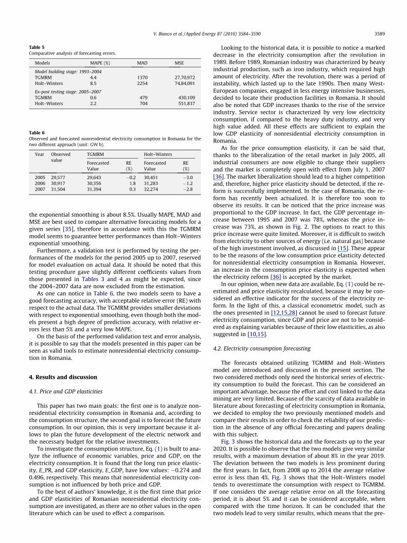
Table 5Comparative analysis of forecasting errors.

Models MAPE (%) MAD MSE

Model building stage: 1993–2004TGMRM 4.4 1370 27,70,972Holt–Winters 8.5 2254 74,84,091

Ex-post testing stage: 2005–2007TGMRM 0.6 479 430,109Holt–Winters 2.2 704 551,837

Table 6Observed and forecasted nonresidential electricity consumption in Romania for thetwo different approach (unit: GW h).

Year Observedvalue

TGMRM Holt–Winters

ForecastedValue

RE(%)

ForecastedValue

RE(%)

2005 29,577 29,643 �0.2 30,451 �3.02006 30,917 30,356 1.8 31,283 �1.22007 31,504 31,394 0.3 32,274 �2.8

V. Bianco et al. / Applied Energy 87 (2010) 3584–3590 3589

the exponential smoothing is about 8.5%. Usually MAPE, MAD andMSE are best used to compare alternative forecasting models for agiven series [35], therefore in accordance with this the TGMRMmodel seems to guarantee better performances than Holt–Wintersexponential smoothing.

Furthermore, a validation test is performed by testing the per-formances of the models for the period 2005 up to 2007, reservedfor model evaluation on actual data. It should be noted that thistesting procedure gave slightly different coefficients values fromthose presented in Tables 3 and 4 as might be expected, sincethe 2004–2007 data are now excluded from the estimation.

As one can notice in Table 6, the two models seem to have agood forecasting accuracy, with acceptable relative error (RE) withrespect to the actual data. The TGMRM provides smaller deviationswith respect to exponential smoothing, even though both the mod-els present a high degree of prediction accuracy, with relative er-rors less than 5% and a very low MAPE.

On the basis of the performed validation test and error analysis,it is possible to say that the models presented in this paper can beseen as valid tools to estimate nonresidential electricity consump-tion in Romania.

4. Results and discussion

4.1. Price and GDP elasticities

This paper has two main goals: the first one is to analyze non-residential electricity consumption in Romania and, according tothe consumption structure, the second goal is to forecast the futureconsumption. In our opinion, this is very important because it al-lows to plan the future development of the electric network andthe necessary budget for the relative investments.

To investigate the consumption structure, Eq. (1) is built to ana-lyze the influence of economic variables, price and GDP, on theelectricity consumption. It is found that the long run price elastic-ity, E_PR, and GDP elasticity, E_GDP, have low values: �0.274 and0.496, respectively. This means that nonresidential electricity con-sumption is not influenced by both price and GDP.

To the best of authors’ knowledge, it is the first time that priceand GDP elasticities of Romanian nonresidential electricity con-sumption are investigated, as there are no other values in the openliterature which can be used to effect a comparison.

Looking to the historical data, it is possible to notice a markeddecrease in the electricity consumption after the revolution in1989. Before 1989, Romanian industry was characterized by heavyindustrial production, such as iron industry, which required highamount of electricity. After the revolution, there was a period ofinstability, which lasted up to the late 1990s. Then many West-European companies, engaged in less energy intensive businesses,decided to locate their production facilities in Romania. It shouldalso be noted that GDP increases thanks to the rise of the serviceindustry. Service sector is characterized by very low electricityconsumption, if compared to the heavy duty industry, and veryhigh value added. All these effects are sufficient to explain thelow GDP elasticity of nonresidential electricity consumption inRomania.

As for the price consumption elasticity, it can be said that,thanks to the liberalization of the retail market in July 2005, allindustrial consumers are now eligible to change their suppliersand the market is completely open with effect from July 1, 2007[36]. The market liberalization should lead to a higher competitionand, therefore, higher price elasticity should be detected, if the re-form is successfully implemented. In the case of Romania, the re-form has recently been actualized. It is therefore too soon toobserve its results. It can be noticed that the price increase wasproportional to the GDP increase. In fact, the GDP percentage in-crease between 1995 and 2007 was 78%, whereas the price in-crease was 73%, as shown in Fig. 2. The options to react to thisprice increase were quite limited. Moreover, it is difficult to switchfrom electricity to other sources of energy (i.e. natural gas) becauseof the high investment involved, as discussed in [15]. These appearto be the reasons of the low consumption price elasticity detectedfor nonresidential electricity consumption in Romania. However,an increase in the consumption price elasticity is expected whenthe electricity reform [36] is accepted by the market.

In our opinion, when new data are available, Eq. (1) could be re-estimated and price elasticity recalculated, because it may be con-sidered an effective indicator for the success of the electricity re-form. In the light of this, a classical econometric model, such asthe ones presented in [12,15,28] cannot be used to forecast futureelectricity consumption, since GDP and price are not to be consid-ered as explaining variables because of their low elasticities, as alsosuggested in [10,15].

4.2. Electricity consumption forecasting

The forecasts obtained utilizing TGMRM and Holt–Wintersmodel are introduced and discussed in the present section. Thetwo considered methods only need the historical series of electric-ity consumption to build the forecast. This can be considered animportant advantage, because the effort and cost linked to the datamining are very limited. Because of the scarcity of data available inliterature about forecasting of electricity consumption in Romania,we decided to employ the two previously mentioned models andcompare their results in order to check the reliability of our predic-tion in the absence of any official forecasting and papers dealingwith this subject.

Fig. 3 shows the historical data and the forecasts up to the year2020. It is possible to observe that the two models give very similarresults, with a maximum deviation of about 8% in the year 2019.The deviation between the two models is less prominent duringthe first years. In fact, from 2008 up to 2014 the average relativeerror is less than 4%. Fig. 3 shows that the Holt–Winters modeltends to overestimate the consumption with respect to TGMRM.If one considers the average relative error on all the forecastingperiod, it is about 5% and it can be considered acceptable, whencompared with the time horizon. It can be concluded that thetwo models lead to very similar results, which means that the pre-

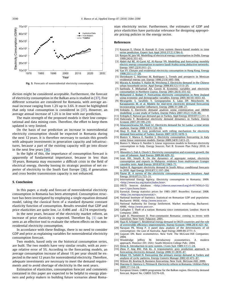
Fig. 3. Forecasts of nonresidential electricity consumption.

3590 V. Bianco et al. / Applied Energy 87 (2010) 3584–3590

diction might be considered acceptable. Furthermore, the forecastof electricity consumption in the Balkan area is studied in [37]. Fivedifferent scenarios are considered for Romania, with average an-nual increase ranging from 1.2% up to 3.6%. It must be highlightedthat only total consumption is considered in [37]. However, anaverage annual increase of 1.2% is in line with our prediction.

The main strength of the proposed models is their low compu-tational and data mining costs. Therefore, the effort to keep themupdated is very limited.

On the basis of our prediction an increase in nonresidentialelectricity consumption should be expected in Romania duringthe next 12 years. It is therefore necessary to sustain this growthwith adequate investments in generation capacity and infrastruc-tures, because a part of the existing capacity will go into disusein the next few years [36].

In the light of this, the importance of consumption forecast isapparently of fundamental importance, because in less than10 years, Romania may encounter a difficult crisis in the field ofelectrical energy, thereby loosing its strategic position of net ex-porter of electricity to the South East Europe [36], if generationand cross border transmission capacity is not enhanced.

5. Conclusion

In this paper, a study and forecast of nonresidential electricityconsumption in Romania has been attempted. Consumption struc-ture has been investigated by employing a single equation demandmodel, taking the classical form of a standard dynamic constantelasticity function of consumption. Results revealed that GDP andprice elasticities are quite low, i.e. 0.496 and �0.274 respectively.

In the next years, because of the electricity market reform, anincrease of price elasticity is expected. Therefore Eq. (1) can beseen as an effective tool to evaluate the reform effects on the non-residential electricity consumption.

In accordance with these findings, there is no need to considerGDP and price as explaining variables for nonresidential electricityconsumption forecast.

Two models, based only on the historical consumption series,are built. The two models have very similar results, with an aver-age relative error of 5%. According to the forecasting models, anaverage consumption increase of about 1% per year should be ex-pected in the next 12 years for nonresidential electricity. Therefore,adequate investments are necessary to meet the demand require-ments and to avoid shortage of electricity in the next years.

Estimation of elasticities, consumption forecast and commentscontained in this paper are expected to be helpful to energy plan-ners and policy makers in building future scenarios about Roma-

nian electricity sector. Furthermore, the estimates of GDP andprice elasticities have particular relevance for designing appropri-ate pricing policies in the energy sector.

References

[1] Kayacan E, Ulutas B, Kaynak O. Grey system theory-based models in timeseries prediction. Expert Syst Appl 2010;37(2):1784–9.

[2] Ranjan M, Jain VK. Modelling of electrical energy consumption in Delhi. Energy1999;24(4):351–61.

[3] Abdel-Aal RE, Al-Garni AZ, Al-Nassar YN. Modelling and forecasting monthlyelectric energy consumption in eastern Saudi Arabia using abductive networks.Energy 1997;22(9):911–21.

[4] Yan YY. Climate and residential electricity consumption in Hong Kong. Energy1998;23(1):17–20.

[5] Sheinbaum C, Martinez M, Rodriguez L. Trends and prospects in Mexicanresidential energy use. Energy 1996;21(6):493–504.

[6] Murata A, Kondou Y, Hailin M, Weisheng Z. Electricity demand in the Chineseurban household-sector. Appl Energy 2008;85(12):1113–25.

[7] Egelioglu F, Mohamad AA, Guven B. Economic variables and electricityconsumption in Northern Cyprus. Energy 2001;26(4):355–62.

[8] Mohamed Z, Bodger P. Forecasting electricity consumption in New Zealandusing economic and demographic variables. Energy 2005;30(10):1833–43.

[9] Mirasgedis S, Sarafidis Y, Georgopoulou E, Lalas DP, Moschovits M,Karaggiannis M, et al. Models for mid-term electricity demand forecastingincorporating weather influences. Energy 2006;31:208–27.

[10] Erdogdu E. Electricity demand analysis using cointegration and ARIMAmodelling: a case study of Turkey. Energy Policy 2007;35(2):1129–46.

[11] Erdogdu E. Natural gas demand gas in Turkey. Appl Energy 2010;87(1):211–9.[12] Halicioglu F. Residential electricity demand dynamics in Turkey. Energy

Econom 2007;29:199–210.[13] Amarawickrama HA, Hunt LC. Electricity demand for Sri Lanka: a time series

analysis. Energy 2008;33(5):724–39.[14] Akay D, Atak M. Grey prediction with rolling mechanism for electricity

demand forecasting of Turkey. Energy 2007;32(9):1670–5.[15] Bianco V, Manca O, Nardini S. Electricity consumption forecasting in Italy

using linear regression models. Energy 2009;34(9):1413–21.[16] Bianco V, Manca O, Nardini S. Linear regression models to forecast electricity

consumption in Italy. Energy Sources, Part B: Econom Plan Policy 2010, inpress.

[17] Abosedra S, Dah A, Ghosh S. Electricity consumption and economic growth, thecase of Lebanon. Appl Energy 2009;86:429–32.

[18] Lean HH, Smyth R. On the dynamics of aggregate output, electricityconsumption and exports in Malaysia: evidence from multivariate Grangercausality tests. Appl Energy 2010;87(6):1963–71.

[19] Inglesi R. Aggregate electricity demand in South Africa: conditional forecaststo 2030. Appl Energy 2010;87(1):197–204.

[20] Payne JE. A survey of the electricity consumption-growth literature. ApplEnergy 2010;87(3):723–31.

[21] International Energy Agency. Electricity consumption in Romania; 2009.<http://www.iea.org/statist/index.htm>.

[22] OECD. Sources database. <http://oberon.sourceoecd.org/vl=917456/cl=32/nw=1/rpsv/home.htm>.

[23] Eurostat. Energy statistics prices for 1985–2007. Bruxelles: Eurostat; 2008.<http://ec.europa.eu/eurostat/>.

[24] National Institute of Statistics. Statistical on Romanian GDP and population.Bucharest: INSSE. <http://www.insse.ro>.

[25] National Authority for Energy Settlement. Market monitoring. Bucharest:ANRE. <http://www.anre.ro>.

[26] Gallagher T. Theft of a nation: Romania since communism. London: Hurst &Company; 2005.

[27] Light D, Phinnemore D. Post-communist Romania: coming to terms withtransition. New York: Palgrave; 2001.

[28] Haas R, Schipper L. Residential energy demand in OECD-countries and the roleof irreversible efficiency improvements. Energy Econom 1998;20(4):421–42.

[29] Narayan PK, Wong P. A panel data analysis of the determinants of oilconsumption: the case of Australia. Appl Energy 2009;86:2771–5.

[30] Gujarati DN. Basic econometrics. New York: The McGraw-Hill Companies;2004.

[31] Wooldridge Jeffrey M. Introductory econometrics. A modernapproach. Florence (KY, USA): South-Western College Pub.; 2004.

[32] Deng JL. Introduction to grey system. J Grey Syst 1989;1(1):1–24.[33] Zhou P, Ang BW, Poh KL. A trigonometric grey prediction approach to

forecasting electricity demand. Energy 2006;31:2839–47.[34] Ediger VS, Tatlidil H. Forecasting the primary energy demand in Turkey and

analysis of cyclic patterns. Energy Convers Manage 2002;43:473–87.[35] Wilson JH, Keating B. Business forecasting. New York: McGraw-Hill; 2009.[36] Diaconu O, Oprescu G, Pittman R. Electricity reform in Romania. Utilities Policy

2009;17:114–24.[37] European Union. CARDS programme for the Balkan region. Electricity demand

forecast. Report No. CARDS 52276-GIS.