Low Cost Inferential Forecasting and Tourism Demand in Accommodation Industry

TOURISMOS: AN INTERNATIONAL MULTIDISCIPLINARY JOURNAL OF TOURISM Volume 4, Number 2, Autumn 2009, pp. 47-68

47

LOW COST INFERENTIAL FORECASTING AND TOURISM DEMAND IN ACCOMMODATION

INDUSTRY

Zaharias Psillakis1

University of Patras

Alkiviadis Panagopoulos Technological Educational Institute of Patras

Dimitris Kanellopoulos Technological Educational Institute of Patras

This paper establishes a low cost inferential model that allows reliable time series forecasts. The model provides a naive unique computationally straightforward approach based on widely-used additive models. It refers to the decomposition of every time series value in “random” components, which are compounded to constitute a “Fibonacci type” predictor random variable. The expected value of this predictor gives a forecast of a future time series value. The standard deviation of the predictor serves to construct a prediction interval at a predefined confidence level. The major features of our model are: forecasting accuracy, simplicity of the implementation technique, generic usefulness, and extremely low cost effort. These features enable our model to be adopted by tourism practitioners on various types of forecasting demands. In this paper, we present an application study to forecast tourism demand that exists in the Greek accommodation industry (i.e. in Greece and in the broad region of Athens). In the application study, two independent approaches have been adopted. In the first approach we implemented our model, and in the second approach we implemented the well-known Box-Jenkins method. Keywords: Time series; forecasting models; Naïve models; ex-post and ex-ante

forecasts; forecast accuracy and validation; tourism demand INTRODUCTION

The importance of tourism industry in world is indisputable. Tourism has become a very competitive business and has a significant impact on

© University of the Aegean. Printed in Greece. Some rights reserved. ISSN: 1790-8418

Zaharias Psillakis, Alkiviadis Panagopoulos & Dimitris Kanellopoulos

48

local economies directly and indirectly. The competitive advantage no longer lies in natural resources only, but increasingly in the level of technology, information and innovation offered. Forecasting is about predicting the behavior of future events (Makridakis & Hibon, 1979; Frees, 1996; Franses, 2004) and plays a significant role in tourism planning. Tourism investments should be based on professional business planning and on achievement vision of the industry future. The tourism industry needs to reduce the risks of poor decisions. One prompt way to reduce this risk is by discerning future events or environments more clearly (Smith, 1995; Burger et al., 2001). Benefits derived from forecasting are imaginable. In the case of forecasts of demands turning out too high, accommodation firms will suffer; there might be, for instance empty rooms in hotels, unoccupied apartments, and so on. If, on the other hand, the case turned out to be that forecasts of demand are too low, then firms will lose opportunities; for example, there may be inadequate hotel accommodation etc. (Chu, 2004). Tourism demand forecasting is as much an art as it is a science. On the other hand, an important aspect of business and economic analysis is the construction of time series models, used for modeling and forecasting of demands in the enterprises domain. As you become familiar with series you are forecasting you gain insights into what makes it tick. Further, tourism demand forecasting is a diverse, dynamic and challengeable process (Frechtling, 2001). A review of the current literature on tourism forecasting is given in (Song & Witt, 2006). Time series forecasts are extrapolations in future times of the available time series values. A good projection should provide a forecaster with a sense of the reliability of the forecast. A convenient way to capture this sense is the prediction interval, which provides a measure of the reliability of the forecast. Further, by varying the desired level of confidence, the length of the prediction interval varies.

In this paper, we establish an operational inferential model that allows low cost reliable time series forecasting. The proposed methodology (described in the next Section) refers to the decomposition of every time series value in three components, namely: 1) the trend component, the 2) cyclical-seasonal component and 3) the residual effect component. The first two components are considered as random variables taking predefined probabilities (weights). By compounding these two random variables, a new random variable (i.e. a predictor) is established as a linear function of the two pre-referred ones. In this linear function, the used coefficients (weights) obey a selected Fibonacci ratio. In this way, first a forecast (an estimate) of the future value of the time series is


49

given by the expected value of the predictor, second a prediction interval is evaluated based on the standard deviation of it. A properly selected length of the latter prediction interval can be used as an estimation of the residual effect. It is worthwhile noticing that the forecast and the accompanied prediction interval of the model require only seven existing time series values, so it is computationally straightforward.

In support of the proposed model, we compare it with the well-known Box-Jenkins method (Box & Jenkins, 1994). The method of Box-Jenkins is chosen, because of its flexibility and generality as it can handle different types of data. Furthermore, it’s frequent use in applied empirical work and its availability in computer packages (e.g. Minitab Release 14, 2002) have contributed much to its popularity. Because of these, it has become a standard and high documented method to compare with, instead of other possible expert methods but of less generality. Chan et al. (1999), Dharmaratne (1995), Turner et al. (1995), Witt et al. (1994), and Witt et al. (2003) compared the Box-Jenkins approach with other modeling techniques.

In Greece, tourism industry constitutes very crucial economic activities and a valuable source of earnings such as an increase of employment, gross domestic product and multiplier effect investments. A key-factor of the Greek tourism industry is its ability to host visitors in various places. Therefore, a desirable task is to forecast monthly and/or annually percentages of occupancy in Greece and in various regions of this country. Potentially, this task leads to more effective use (allocation) of the available sources for the Greece visitors.

Notation ≡ implies an identity or definition ≈ implies approximately – equal s- implies "statistical (ly)" r.v. random variable(s) E(X) s-Expected value (mean, average) of the r.v. X V(X) Variance of the r. v. X σ(X) Standard deviation of the r.v. X; σ(Χ) = V(X) fn = O (gn) implies fn ∈O (gn) ≡ {hn: there exist positive constants c

and n0 such that 0 ≤ hn ≤ c gn for all n ≥ n0} fn = Ω (gn) implies fn ∈Ω (gn) ≡ {hn: there exist positive constants c

and n0 such that 0 ≤ c gn ≤ hn for all n ≥ n0} I(.) Indicator function: I(True) = 1, I(False) = 0.


50

Definitions – Assumptions 1. A time series is a collection of data obtained by observing a response

variable sequentially at periodic points in time (e.g. on weekly, monthly, quarterly, or annually basis).

2. It is common practice to consider as a reference cycle or period p, a year for monthly (p=12) or quarterly data (p=4) and a five or ten years period for annually recorded data.

3. The repeated observations on a variable produce a time series, the variable is called a time series variable. We use wm, to denote the values of the variable at time m. The data consists of N equally spaced values w1, w2,…, wN.

4. In practical applications, the main objective of times series is to forecast (predict or estimate) some future value or values wm, m≥ N+1 of the series. Ex-post forecasting is a type of forecasting that is based on existing values ,,...,

21 mm ww (1≤ m1<m2<N) and is

checked against existing values ,,...,43 mm ww (m2 <m3<m4≤ N) of

the time series, in order to evaluate some measure of the forecasting accuracy and/or validate the forecasts. Ex-ante forecasts predict future value (values) wm, m> N of a time series beyond the time period of the existing data values wm, m=1,2...,N. In such cases, there are not available data for comparison and there is only a posteori forecasts validation – once the corresponding data become available, instead of a priori validation of ex-post forecasts. Usually ex-ante forecasts are done for one reference period ahead.

5. Forecast error (residual) is defined as the actual value wm minus the forecasted value (or fitted), fm of the time series variable at time m, namely: em = wm - fm.

6. To analyze the relative performance of several consecutive ex-post forecasts in the time window m1 to m (1 ≤ m1 <m ≤ N), the popular root mean squared error (RMSE) criterion is used. For a such time-window the RMSE

1mm ,r (or mr if m1 is predefined) is calculated:

The rest of this paper is organized as follows. The next section

introduces the proposed model. Then, we present an application study of

.e1mm

1,r2

1m

mn

2n

1mm

1

1

+−= ∑

=


51

the forecasting model for accommodation demand in Greece. This application study is referred to accommodation occupancies in Greece (case 1) and in broad region of Athens as a special region of Greece (case 2). The data refers to the monthly percentages of occupancy of all types of tourist accommodation (except camping sites) of both foreign and domestic tourists. The model is applied to these data and its results are compared to those of the Box-Jenkins method. We present and discuss the above results. Finally, in the last section we conclude the paper and give hints for further research. THE PROPOSED MODEL Notation – assumptions – definitions mp 1+5p; a lower threshold value of m. It is assumed

m ≥ mp, unless otherwise specified Xm, Ym, Y'm random variables ´ a prime over a token implies the usage of r. v. Y'm F {0.146, 0.236, 0.382, 0.618, 0.764, 0.854}; a set of

Fibonacci ratios Fm( φ ), Fm }1or 1F mmmmm Υ′φ−+ΧφΥφ−+Χφ≡φ )({)()( . A

“predictor” r.v. such that: fm ≡ E[Fm( φ )] predicts (forecasts) the "unknown" value of wm . The parameter φ ∈F can be omitted, when it is obvious or predefined

k a real number larger or equal to 1 α(k), α )/( 2k11− ; a confidence level (lm( φ ), um( φ ))α a prediction interval for wm with confidence level α. lm(

φ ) = lm ≡ fm - k σ(Fm), um ( φ ) = um ≡ fm + k σ(Fm) Ζm( φ ), Ζm Ι ("the interval (lm, um)α contains wm "); a binary r.v. bm( φ ), bm }l 2lub mmmm )(/{)}()({)( φφ−φ≡φ for lm( φ ) ≠ 0

An upper bound of the relative error (for wm ≠ 0),

mmm weE /≡

mmm, cc1

),(φ

∑=+−

m

1mn nZ11mm

1 cumulative number of times that

consecutive wm values are containing into (lm, um) for a


52

time window m1 to m. A commonly used criterion to analyze ex-post forecasts of an inferential model.

Model’s description

Researchers often describe the nature of a time series wm by

identifying three kinds of change (or variation) of the time series values. These three components are commonly known as: (1) trend component, tm, (2) cyclical-seasonal component sm, and (3) residual effect, hm (Mendenhall & Sincich, 1996). To obtain forecasts, a model (that can be projected into the future) must be adopted to describe the time series. One of the most widely used models is the additive model

wm = tm + sm + hm (1)

or alternatively the log-additive (or multiplicative) model

ln(wm) = ln(tm) + ln(sm) + ln(hm) (1')

depending on the scale of the variation of the values of the underlying time series variable. Since business and economic cycles last usually 5 years, and seasonal data are usually related to their predecessor and successor ones, to simulate eq.(1) the following methodology is used.

Trend component: Let Xm denotes a r.v. simulating the "random" behavior of the trend component of a time series at time m. Suppose that Xm takes the value xm,i with probability (weight) gi, i=1,2,3,4,5 given in the Table 1.

Table 1. Values and distribution of r.v. Xm

i 1 2 3 4 5 xm,i wm-5p wm-4p wm-3p wm-2p wm-p gi 1/12 1/12 2/12 3/12 5/12

This scheme obeys a Fibonacci-type memory rule and uses values of

the time series of the same periodicity (lag). It gives more weight (memory) in the most recent used time series value.

Cyclical-seasonal component: To simulate the "random" behavior of the cyclical-seasonal component of a time series at time m, we define the r.v. Ym {or alternatively Y'm} with probability (weight) gj, j=1,2,3 given in the Table 2.


53

Table 2. Values and distribution of r.v. Ym {or Y’m} j 1 2 3 ym,j wm-p-1 wm-p wm-p+1 , if m<N + p wN+1 , if m=N + p y'm,j wm-1 wm-p wm-p+1 gj 1/4 2/4 1/4

This scheme obeys a Fibonacci-type memory rule too, and takes into

account data with the same periodicity or cyclicality of m and neighbor values of it with correlated seasonality. This means that we use: (a) r.v. Ym {or r.v. Y'm} for one-step ahead forecasting (one time series value ahead) and (b) r.v. Ym for one-period ahead forecasting (per whole reference cycle p).

Based on r.v. Xm and Ym {or Y'm}, a r.v. Fm(φ ) (with φ F∈ ) can be defined as a Fibonacci weighed average of these. Fm(φ ) simulate the "random" behavior of the time series value wm except the residual effect hm, for every m ≥ m p. From elementary probability theory (Ross, 1998) it is derived:

fm ≈ wm (2)

Pr (|Fm-fm| < k σ(Fm)) ≥2

11k

− , (3)

k σ(Fm) ≈ |em| ≈ |hm|. (4)

Remark 1: For every m the forecast and the accompanied prediction interval with confidence at least )%k/11( 2− of the model require only seven existing time series values. The computation of σ(Fm), is based on an estimation of the correlation between r.v. Xm and Ym {or Y'm} and it is given in the Appendix. The overall scheme is computationally straightforward and can be computed simply by the use of a normal hand calculator.

Remark 2: The quantity kσ(Fm) gives by its definition an estimate of the absolute value of the unknown error em or in other words gives an estimate of the order of magnitude of the absolute value of the random factor in the time series, namely of the residual effect. Let 2=∗k be a threshold value of k, so that a prediction interval (l*m, u*m) with 50% at least confidence it will contain the unknown value wm. The quantities k* σ(Fm) and (l*m, u*m) do not give accurate estimate and prediction interval respectively for the "random" residual effect component of wm, but rather


54

give estimates about the order of its magnitude. To get more accurate estimates, we ought to use larger values of k > k*.

Remark 3: In ex-ante forecasts (in which there is only a posteori validation) important role has the estimate bm. It gives a priori a sense of an estimate of the order of the worst possible relative error that is committed in forecasting wm by fm = (lm+um)/2 (Makri & Psillakis, 1997) for every k ≥ k* and φ F∈ .

Model’s forecasting evaluation

In modeling of time series data, we need to judge the accuracy of

forecasts and/or their prediction intervals. To address these concerns, we will use an out-of-sample validation technique. Definitions – assumptions 1. Random variables Xm, Ym define model 1, whereas r.v. Xm and Y'm

define model 2. 2. A model’s version depends on φ F∈ that is used in it. 3. With an out-of-sample validation, we fit various versions of a model

to one portion of the available data – the model’s development subsample and test or validate the best candidate versions and/or models on a second portion – the validation subsample, of the available data.

4. The data in the model specification sample (the development subsample) are somehow similar to the out-of-sample data.

Remarks

• Assumption 4 is crucial, because if it is not hold, then there is no point in spending time on the construction of time series model.

• Definition 3 implies that if all forecasts are too high or too low, it would obviously wish the forecasting model to be re–specified.

Forecasting procedure

To make ex-post forecasts evaluation and finally ex-ante forecasts the following two-step process is provided. • Step1: Suppose there are available N = n1 + n2 time series data, then

the first n1 = mp data are used to specify the model (1 or 2) and estimate its parameter φ , and the last n2 = N - n1 data are used to


55

evaluate out-of-sample forecasting performance according to the minimum

1,nNr or the maximum 1,nNc .

• Step2: When the forecasting performance of a version of model 1 is satisfactory, we generate (ex-ante) forecasts and the accompanied relative error estimates bm, for the unknown data at times N+1, N+2, …N+n3, with n3 = tp, t ≥ 1. Obviously, these forecasts can only be evaluated once, the corresponding n3 data values become available.

Remark: This forecasting procedure depends on the selected value of parameter φ F∈ . For every data set we can find the optimum φ = φ * with respect of a predefined criterion. But, it is well known that a model that validates best is not necessarily the one that forecasts best. Simulated studies of the model on various data sets recommend that the value φ = 0.618 generally gives acceptable results and waist time and cost. FORECASTING TOURISM DEMAND IN ACCOMMODATION INDUSTRY IN GREECE

The Greek National Tourist Organization (GNTO) is convinced that Greece can no longer be a destination providing "sun, sea and sand” vacations. There is a need to attract more high spending visitors and to make more effective use of the comparative advantages of the different regions of Greece. A contemporary political promotion of tourism is indispensable. For example, we need promotion campaigns for Greek destinations that will project and promote alternative forms of tourism. Some of the major problems confronted by the Greek tourist authorities are: 1) seasonality of tourism employment, 2) unequal standards of tourist services, 3) development of para-hotel economy, and 4) the environmental problems. In Greece, the seasonal distribution of tourism has brought several negative effects: a) significant increases of unemployment during the low–season period, b) high concentration of tourists during the months of the high–season in specific degradation, c) the absorption of the labor force from other sectors of the economy, and d) the creation of inflationary prices as a result of the increased demand for tourist services and products. To combat the seasonal problem of the tourist industry, some significant strategies (Panagopoulos, 2005) are necessary: variation of the tourism product–mix, diversification of the market, differential pricing strategies, state encouragement, alternative types of tourism and balanced regional tourist development. In order to achieve a more balanced tourist flow, the GNTO is promoting Greece’s winter skiing facilities, conference tourism, hydrotherapy holidays, time–


56

sharing tourism, etc. For example, the promotion of winter tourism and the subsidies to private tourism operators could increase tourists’ arrival during the low season period.

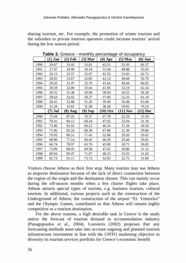
Table 3. Greece - monthly percentage of occupancy

(1) Jan (2) Feb (3) Mar (4) Apr (5) May (6) Jun 1990 29.67 33.42 33.81 43.51 55.93 66.37 1991 27.47 28.90 30.54 31.94 48.88 55.93 1992 30.13 33.57 32.07 41.55 53.83 62.73 1993 28.92 33.67 32.85 42.14 49.68 56.79 1994 29.26 32.47 32.76 41.64 58.44 66.02 1995 28.59 32.89 33.04 41.95 53.19 61.54 1996 28.35 31.46 30.00 38.94 50.55 56.28 1997 29.63 32.02 30.37 37.86 52.33 61.24 1998 30.41 32.88 31.20 39.40 56.08 65.60 1999 31.28 33.81 31.08 38.58 59.05 70.24

(7) Jul (8) Aug (9) Sep (10) Oct (11) Nov (12) Dec 1990 75.94 87.43 70.37 47.78 32.29 31.94 1991 70.41 84.13 68.54 47.92 32.04 31.39 1992 73.96 82.65 68.22 46.16 31.26 30.56 1993 71.96 82.16 68.38 47.88 31.30 29.86 1994 76.83 86.51 71.43 52.68 29.50 29.62 1995 68.90 77.14 66.45 46.39 29.46 30.81 1996 66.74 78.97 63.76 45.00 28.71 26.83 1997 73.99 88.05 69.38 47.62 30.80 31.15 1998 80.94 90.47 71.07 48.25 33.55 31.02 1999 82.73 91.11 73.73 52.93 32.75 31.89

Visitors choose Athens as their first stop. Many tourists may use Athens as stopover destination because of the lack of direct connection between the region of the origin and the destination chosen. This can mainly occur during the off-season months when a few charter flights take place. Athens attracts special types of tourists, e.g. business tourism, cultural tourism. In additional, various projects such as the construction of the Underground of Athens, the construction of the airport “El. Venizelos” and the Olympic Games, contributed so that Athens will remain highly competitive as a tourism destination.

For the above reasons, a high desirable task in Greece is the study and/or the forecast of tourism demand in accommodation industry (Panagopoulos et al., 2004). Louvieris (2002) proposes that any forecasting methods must take into account ongoing and planned tourism infrastructure investment in line with the GNTO marketing objective to diversity its tourism services portfolio for Greece’s economic benefit


57

Figure 1. Greece –Timeplot 1990(1)-1999(12)

Table 4. Athens- monthly percentage of occupancy

(1) Jan (2) Feb (3) Mar (4) Apr (5) May (6) Jun 1990 32,30 34,77 41,07 51,21 47,40 49,16 1991 28,54 26,89 30,82 33,92 40,19 38,90 1992 32,72 37,84 38,52 44,06 41,90 45,72 1993 32,86 37,91 46,49 45,15 46,75 45,62 1994 32,78 38,59 46,04 45,47 46,86 52,39 1995 32,69 38,52 46,20 45,41 46,91 51,76 1996 33,95 38,05 51,19 49,34 54,58 49,70 1997 33,76 40,45 46,11 48,52 42,52 50,68 1998 37,77 40,85 47,41 50,81 54,96 51,42 1999 39,38 44,08 50,67 47,95 49,69 46,58

(7) Jul (8) Aug (9) Sep (10) Oct (11) Nov (12)Dec 1990 53,25 62,35 54,67 44,39 37,86 32,52 1991 45,97 54,75 51,80 43,17 36,78 32,68 1992 51,40 58,05 54,71 45,36 35,14 31,27 1993 51,44 58,05 55,79 45,20 37,76 32,15 1994 51,85 57,65 56,30 45,20 37,74 32,04 1995 52,75 58,34 56,46 45,42 39,63 32,05 1996 49,67 53,49 53,21 50,70 40,26 32,03 1997 50,96 60,84 56,80 51,47 40,26 35,46 1998 50,91 60,03 58,32 52,48 46,26 36,91 1999 50,96 49,94 50,89 48,02 45,90 37,46

0,00

10,00

20,00

30,00

40,00

50,00

60,00

70,00

80,00

90,00

100,00

1 13 25 37 49 61 73 85 97 109

m (months)

Occ

upan

cy%


58

Figure 2. Athens –Timeplot 1990(1)-1999(12)

. Hereafter, we present an application study of the proposed model

using tourism data concerning the monthly percentages of occupancy of all types of tourism accommodation (expect camping sites) in Greece (case study 1) and in the broad region of Athens (case study 2). The data were derived from the official records of the Greek Statistical Office and involve the monthly occupancy of all the tourist accommodation both foreign and domestic tourists for the time period January 1990 {or 1990(1)} until December 1999 {or 1999(12)}. At this point, we underline that the GNTO has not released any similar data for the period 2000 until now. The proposed model is applied to these data and its results are compared to those of the well known Box-Jenkins method, which is a standard method in the time series domain. This study reveals the simplicity and the potential significant use of our model and verifies its high reliability.

The data and their coding

The monthly percentages of occupancy for Greece are presented in

Table 3 (Greece) and in Table 4 (broad region of Athens). The data were coded from w1(1990(1)) to wN(1999(12)) with N=120, so that a time series w1, w2, …, wN was derived for further processing. Figs. 1, 2 are illustrations of the time plot of our data.

Figure 3. Greece 1995(1) - 1999(12)


59

RESULTS AND DISCUSSION Case Study 1: Greece

We used our model (with φ = 0.618) and the Box–Jenkins method in

order to forecast (predict) the monthly percentage (p = 12) of accommodation occupancy in Greece for the year 2000 – that is to make 12 ex-ante forecasts. In order to have the ability to check the forecasts and the prediction intervals accuracy using real data, we made ex-post forecasts via our model (1 and 2). These forecasts correspond to time series values: w61 (1995(1)) to w120 (1999(12)). This means that the values (which are going to be forecasted) were excluded from our data set. Therefore, our model is used without these observations of the time series values and then we made the forecasts. After that, these forecasts were compared with the real data that we kept outside from this procedure.

Figure 3 displays the cumulative (running or moving) RMSE, rm (model 1, solid line) and r'm (model 2, dotted line) for m=61 to 120. Model 2 gives in the most cases smaller RMSE - thus more accurate forecast – owing that is used value wm-1 instead of value wm-p-1 (used in model 1). From the curves of Figure 3 there is an evidence that r'm = O ( rm).

Figure 4. Greece 1995(1)-1999(12), k=1.4142


60

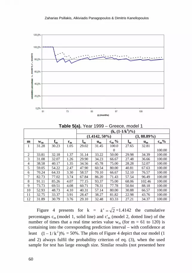
Table 5(a). Year 1999 – Greece, model 1 (k, (1-1/k2)%)

(1.4142, 50%) (3, 88.89%) m wm fm rm lm um cm % lm um cm% 1 31.28 30.23 1.05 29.02 31.45 100.0

0 27.65 32.81

100.00 2 33.81 32.18 1.37 31.14 33.22 50.00 29.98 34.39 100.00 3 31.08 32.07 1.26 29.90 34.23 66.67 27.48 36.66 100.00 4 38.58 40.17 1.35 34.56 45.78 75.00 28.28 52.07 100.00 5 59.05 54.22 2.47 47.90 60.54 80.00 40.81 67.63 100.00 6 70.24 64.33 3.30 58.57 70.10 66.67 52.10 76.57 100.00 7 82.73 77.02 3.74 67.84 86.20 71.43 57.54 96.49 100.00 8 91.11 85.26 4.07 77.15 93.37 75.00 68.06 102.46 100.00 9 73.73 69.51 4.08 60.71 78.31 77.78 50.84 88.18 100.00

10 52.93 48.73 4.10 40.31 57.14 80.00 30.88 66.57 100.00 11 32.75 33.37 3.91 28.47 38.27 81.82 22.98 43.76 100.00 12 31.89 30.79 3.76 29.10 32.48 83.33 27.21 34.37 100.00

Figure 4 presents for k = 2=∗k =1.4142 the cumulative

percentages cm (model 1, solid line) and c'm (model 2, dotted line) of the number of times that a real time series value wm (for m = 61 to 120) is containing into the corresponding prediction interval – with confidence at least )%k/11( 2− = 50%. The plots of Figure 4 depict that our model (1 and 2) always fulfil the probability criterion of eq. (3), when the used sample for test has large enough size. Similar results (not presented here


61

but are available from the authors on request) for values k > ∗k confirm the same token. Furthermore as it can easily seen c'm = Ω (cm). Same comments (as in the case of RMSE – Fig. 3) are also true for cm and c'm.

Table 5(b). Year 1999 – Greece, model 2

(k, (1-1/k2)%) (1.4142, 50%) (3, 88.89%)

m wm fm rm lm um cm % lm um cm % 1 31.28 30.22 1.06 29.01 31.43 100.00 27.65 32.79 100.00 2 33.81 32.27 1.32 31.35 33.19 50.00 30.31 34.22 100.00 3 31.08 32.16 1.25 30.04 34.27 66.67 27.66 36.65 100.00 4 38.58 40.16 1.34 34.53 45.79 75.00 28.23 52.09 100.00 5 59.05 54.14 2.50 47.65 60.63 80.00 40.37 67.91 100.00 6 70.24 64.62 3.24 59.27 69.97 66.67 53.27 75.96 100.00 7 82.73 77.46 3.60 69.16 85.76 71.43 59.86 95.06 100.00 8 91.11 85.43 3.92 77.33 93.53 75.00 68.24 102.62 100.00 9 73.73 69.57 3.95 60.65 78.49 77.78 50.66 88.49 100.00

10 52.93 48.98 3.95 40.02 57.94 80.00 29.96 68.00 100.00 11 32.75 33.82 3.78 27.84 39.79 81.82 21.14 46.49 100.00 12 31.89 30.72 3.63 29.09 32.35 83.33 27.26 34.17 100.00 Table 5a (model 1) and Table 5b (model 2) present results of the model application to ex-post forecasts and give prediction intervals for monthly percentages of occupancy for the year 1999 from month 1(Jan) to 12(Dec). To take these results the last 12 observations namely w109, w110, …,w120, were excluded - as usually- from the time series values. We forecast values without these observations and then take forecasts for this latter interval 1999(1-12). Finally, we compare these forecasts with the data that we kept outside of this procedure. The data of Tables are quite self-explained and confirm the comments on Figures 3 and 4.

To compare our results, a Box-Jenkins model was used and its results are presented in Table 7. The implementation of the Box-Jenkins method is a very hard programming task or alternatively requires the usage of a high sophisticated computer package. For this task, we used the Minitab Rel. 14 package and after a series of tests, we concluded to the following SARIMA model (1,1,1) (1,0,1)12, viz. one seasonal MA (moving average) and one seasonal AR (autoregressive) parameters for the seasonal part of the model. For the non seasonal part of the model we use one MA and one AR parameters. Hence, the final accepted model has all of its parameters statistically significant and gives residuals normally distributed (Table 6). The used format in Table 6 is similar to the output of the Minitab Rel. 14 package. A simple comparison of the results


62

presented in Tables 5 and 7 reveals the potential performance of our model and confirms its reliability.

Table 6. The model SARIMA (1,1,1) (1,0,1)12 : Greece Type Coef StDev T P AR 1 0.4495 0.1366 3.29 0.001 SAR 12 0.9993 0.0027 375.67 0.000 MA 1 0.8273 0.0854 9.69 0.000 SMA 12 0.8590 0.0811 10.59 0.000 Differencing : 1 regular difference Number of observations: Original series 120, after differencing 119 Residuals: SS = 0.239063 (back forecasts excluded), MS = 0.002079 DF = 115

Modified Box-Pierce (Ljung-Box) Chi-Square statistic Lag 12 24 36 48 Chi-Square 7.1 12.3 23.0 39.4 DF 8 20 32 44 P-Value 0.521 0.906 0.878 0.671

Table 7. Year 1999 – Greece, Box - Jenkins

95% limits m wm fm rm lm um cm % 1 31.28 30.30 0.98 27.71 33.13 100.00 2 33.81 33.56 0.72 30.20 37.28 100.00 3 31.08 32.75 1.13 29.26 36.66 100.00 4 38.58 40.98 1.55 36.43 46.10 100.00 5 59.05 55.37 2.15 49.04 62.53 100.00 6 70.24 63.94 3.24 56.42 72.45 100.00 7 82.73 76.31 3.85 67.13 86.75 100.00 8 91.11 87.33 3.85 76.58 99.58 100.00 9 73.73 71.05 3.73 62.12 81.26 100.00

10 52.93 49.55 3.70 43.20 56.84 100.00 11 32.75 32.13 3.53 27.93 36.96 100.00 12 31.89 31.27 3.39 27.11 36.07 100.00

Finally, Table 8 presents ex-ante forecasts and accompanied

prediction intervals for the monthly percentages for the year 2000. The results of our model and those of a Box–Jenkins method are of the same order of magnitude.


63

Table 8. Year 2000 – Greece

Box-Jenkins model Our model 95% limits (1.4142, 50%) (3, 88.89%)

m fm lm um fm lm um bm% lm um 1 31.31 28.63 34.23 30.90 29.42 32.39 5.05 27.75 34.06 2 34.56 31.11 38.40 32.81 31.43 34.19 4.39 29.89 35.73 3 33.46 29.89 37.45 32.05 30.21 33.89 6.09 28.14 35.96 4 41.81 37.17 47.03 40.06 33.97 46.16 17.14 27.13 53.00 5 57.48 50.90 64.91 56.27 47.64 64.91 18.13 37.95 74.60 6 66.64 58.81 75.52 67.55 59.13 75.98 14.24 49.68 85.43 7 79.38 69.83 90.24 79.63 70.72 88.53 12.59 60.72 98.53 8 90.35 79.23 103.03 86.89 79.12 94.66 9.82 70.40 103.38 9 73.46 64.23 84.02 71.66 61.86 81.45 15.83 50.88 92.43

10 51.45 44.86 59.02 50.97 40.96 60.99 24.45 29.73 72.22 11 33.15 28.82 38.14 34.14 28.31 39.97 20.59 21.77 46.51 12 32.27 27.97 37.22 31.35 30.05 32.65 4.33 28.59 34.12

Table 9. The model SARIMA (1,0,0) (1,0,2)12 : Athens

The model SARIMA (1,0,0) (1,0,2)12 : Athens Type Coef StDev T P AR 1 0.6360 0.0748 8.50 0.000 SAR 12 1.0017 0.0067 150.53 0.000 SMA 12 0.8048 0.1007 8.00 0.000 SMA 24 -0.2074 0.1043 -1.99 0.049 Number of observations : Original series 120, after differencing 119 Residuals: SS = 967.554 (back forecasts excluded), MS = 8.341 DF = 116

Modified Box-Pierce (Ljung-Box) Chi-Square statistic Lag 12 24 36 48 Chi-Square 19.7 35.2 39.7 55.5 DF 8 20 32 44 P-Value 0.012 0.019 0.163 0.115 Case study 2: Athens

In a similar way to compare our results, we used a Box-Jenkins model and its results are presented in Table 10. For this task, we used also the Minitab Rel.14. The final accepted model has all of its parameters statistically significant and gives residuals normally distributed (Table 9). Finally, Table 10 presents ex-ante forecasts and accompanied prediction intervals for the monthly percentages for the year 2000. The results of our model and those of a Box–Jenkins method are of the same order of magnitude.


64

Table 10. Year 2000 – Athens

Box-Jenkins model Our model 95% limits (1.4142, 50%) (3, 88.89%)

m fm lm um fm lm um bm% lm um 1 36.02 28.60 43.45 38.14 34.52 41.76 10.49 30.47 45.81 2 40.58 33.12 48.04 42.79 38.81 46.77 10.25 34.36 51.22 3 48.06 40.59 55.54 48.60 45.51 51.70 6.80 42.04 55.17 4 49.70 42.22 57.18 48.82 47.09 50.55 3.52 45.15 52.49 5 50.46 42.98 57.94 49.41 45.35 53.47 8.95 40.79 58.03 6 51.27 43.79 58.76 48.89 46.42 51.36 5.32 43.66 54.13 7 53.30 45.82 60.78 50.46 49.21 51.72 2.55 47.80 53.13 8 59.28 51.80 66.77 53.43 48.97 57.88 9.10 43.98 62.87 9 57.06 49.58 64.55 52.69 49.25 56.13 6.98 45.39 59.98

10 51.43 43.95 58.92 49.14 46.73 51.55 5.16 44.04 54.24 11 42.81 35.33 50.29 44.16 39.78 48.53 11.00 34.88 53.44 12 35.29 27.81 42.78 37.48 34.16 40.80 9.72 30.44 44.53 Concluding remarks

We conclude that both models (i.e. our model and the Box-Jenkins

model) present the same order of accuracy in both case studies. However, our model has low cost effort as it requires only seven existing time series values. The simplicity of its implementation technique enables its usage by tourism practitioners via an available spreadsheet package or even a hand calculator. On the other hand, the Box-Jenkins model requires a larger number of observations and the usage of a high sophisticated computer package. CONCLUSIONS AND FURTHER RESEARCH

The purpose of this paper is two fold. Firstly, we introduced a naive low cost inferential model, and secondly using this model we studied and/or forecasted real-world tourism data referring to accommodation in Greece and its capital Athens. The first task was to introduce the model. The novel idea behind the model’s establishment is the definition of a “Fibonacci type” predictor random variable, whose mean value forecasts a future value of time series variable. Furthermore, the standard deviation of the predictor serves to construct a prediction interval for the ″unknown″ value of the preferred variable. The key-point to estimate this prediction interval is an approximate computation of the standard deviation of the predictor. The major features of our model are: 1) forecasting accuracy, 2) simplicity of the implementation technique, 3) generic usefulness, and 4) extremely low cost effort. These features


65

enable our model to be adopted by tourism practitioners on various types of forecasting demands.

The second task involved the usage of our model into tourism demand concerning accommodation. This task was obtained by two independent approaches. The first approach adopted our model that requires only the potential use of a spreadsheet package. In the second approach, we implemented the Box-Jenkins method that requires the usage of a high sophisticated computer package. After the completion of this second task, we evaluated the forecasts of the two methods and we found them similar. By this study, we verify the performance of our model on a set of real-world tourism data. In addition, we checked the reliability and its low cost aspects by comparing it to a standard method.

A possible extension of the proposed model could be considered the introduction of a ″corrector″ that corrects the predictions of the ″predictor″ Fm. Corrector’s definition could be based on a regression in a scatter diagram formed between selected sets of values of wm and fm. To this direction, drafted results are very encouraged. We could use the primitive and/or the corrected scheme of our model on longitudinal data, for further forecasting studies. For example, the under study data could be derived from the travel demand domain (e.g. tourist flows to various tourism destinations). REFERENCES Box, G.E.P. & Jenkins, G.M. (1994). Time Series Analysis: Forecasting and

Control, (3rd ed.). New Jersey, Prentice Hall. Burger, C.J.S.C., Dohnal, M., Kathrada, M. & Law, R. (2001). A practitioner

guide to time-series methods for tourism demand forecasting-a case study of Durban, South Africa. Tourism Management, Vol. 22, pp.403-409.

Chan, Y. M., Hui, T. K. & Yuen, E. (1999). Modelling the impact of sudden environmental changes on visitor arrival forecasts: the case of the Gulf war. Journal of Travel Research, Vol. 37, No.4, pp.391-394.

Chu, F. (2004) Forecasting tourism demand: a cubic polynomial approach. Tourism Management, Vol. 25, pp.209-218.

Dharmaratne, G.S. (1995). Forecasting tourist arrivals. Annals of Tourism Research, Vol. 22, No.4, pp.804-818.

Franses, P.H. (2004). Time series models for business and economic forecasting. Cambridge, University Press.

Frechtling, D.C. (2001). Forecasting tourism demand: methods and strategies. Oxford, Butterworth Heinemann.

Frees, E.W. (1996). Data Analysis Using Regression Models - The Business Perspective. New York, Prentice Hall.

GNTO: Greek National Tourism Organization. Annual Report 1990-1999.


66

Louvieris, P. (2002). Forecasting international tourism demand for Greece: A contingency approach (using Cyberfilter and ARIMA model). Journal of Travel and Tourism marketing, Vol. 13, pp.21-40.

Makri, F.S. & Psillakis, Z.M. (1997). Bounds for reliability of k-within connected–(r,s)-out-of-(m,n) failure systems. Microelectronics and Reliability, Vol. 37, No.8, pp.1217-1224.

Makridakis, S. & Hibon, M. (1979). Accuracy of forecasting: An empirical investigation. Journal of the Royal Statistical Society A, Vol.142, pp.97-145.

Mendenhall, W. & Sincich, T. (1996). A Second course in Statistics – Regression Analysis (5th ed.). New Jersey, Prentice Hall.

Minitab Release 14. (2002). Statistical software for windows. Panagopoulos, A.A. (2005). A statistical model of tourism (development) in

Greece within the framework of European Union (1990-1999): the seasonality effect. Unpublished Phd Dissertation (in Greek), University of Piraeus, Greece.

Panagopoulos, A., Psillakis, Z. & Kanellopoulos, D. (2004). A low cost reliable forecasting model of tourism data. In F.D. Pineda & C.A. Brebbia (Eds). Sustainable Tourism (pp.343-352), Southampton: WIT Press.

Ross, S. (1998). A first course in probability. New Jersey, Prentice Hall. Smith, S.J. (1995). Tourism analysis: A handbook. London, Longman. Song, H. & Witt, S.F. (2006). Forecasting international tourism flows to Macau.

Tourism Management, Vol. 27, No.2, pp.214-224. Turner, L.W., Kulendran, N. & Pergat, V. (1995). Forecasting New Zealand

tourism demand with aggregated data. Tourism Economics, Vol. 1, No.1, pp.51-69.

Witt, C.A., Witt, S. F. & Wilson, N. (1994). Forecasting international tourist flows. Annals of Tourism Research, Vol.21, No.3, pp.612-628.

Witt, S.F., Song, H. & Louvieris, P. (2003). Statistical testing in forecasting model selection. Journal of Travel Research, Vol. 42, pp.151-158.

APPENDIX

σ(Fm)’s computation is based on an estimate of the covariance of r.v.

Xm and Ym {or Y´m }. Because of r.v. Xm and Ym {or Y´m } are depended, the main problem to compute σ(Fm) is the following: The marginal distributions of the r.v. Xm and Ym {or Y´m } are known by their definitions, but their joint distribution is unknown. Hence, the exact evaluation of their covariance is not possible at a first sight. However, this obstacle can be over-passed approximately: the behavior of r.v. Xm and Ym {or Y´m } is imitated by two regression lines that fit the pairs of values (i, xm,i), i=1,2,…,5 and (j, ym,j), j=1,2,3 {or (j, y´m,j), j=1,2,3}


67

respectively. Let X mb and Y mb {or Y mb ′ } be their slopes. Therefore,

their correlation ( )mm

Y,Χρ or { ( )}mm

Y,Χ ′ρ can be approximated by

( )

+

−−≅ρYX

YX

mm

mmm bb

bbY1

1tancos,Χ m

or alternatively,

( )

+

−−≅′ρ′

′

YX

YX

mm

mmm bb

bbY1

1tancos,Χ m

Hence,

( )mm YY ,Χ)Υ()Χ(),Χ(cov mmmm ρσσ≅

or alternatively

( )mm YY ′ρ′σσ≅′ ,Χ)Υ()Χ(),Χ(cov mmmm.

By the definition of r.v. Fm it holds

),cov()()()()()()( mmmmmm YVVFFV Χφ−φ+Υφ−+Χφ=σ≡ 122122

or alternatively

),cov()()()()()()( mmmmmm YVVFFV ′Χφ−φ+Υφ−+Χφ=σ≡ 122122

Therefore, the result follows.

SUBMITTED: AUGUST 2008 REVISION SUBMITTED: DECEMBER 2008 2nd REVISION SUBMITTED: FEBRURY 2009 ACCEPTED: APRIL 2009 REFEREED ANONYMOUSLY


68

Zaharias Psillakis ([email protected]) is an Assistant Professor at the University of Patras, Department of Physics, Patras, GR 26500, Greece.

Alkiviadis Panagopoulos ([email protected]) is an Associate Professor at the Technological Educational Institute of Patras, Department of Tourism Management, Patras, GR 26334 Greece.

Dimitris Kanellopoulos ([email protected]) is a Lecturer at the Technological Educational Institute of Patras, Department of Tourism Management, Patras, GR 26334, Greece.

mailto:[email protected]�



Low Cost Inferential Forecasting and Tourism Demand in Accommodation Industry

Documents

Transcript of Low Cost Inferential Forecasting and Tourism Demand in Accommodation Industry