5879 Demand forecasting technical note
69
Demand forecasting technical note Planning and Regulation Route Planning New Lines Programme
-
Upload
independent -
Category
Documents
-
view
0 -
download
0
Transcript of 5879 Demand forecasting technical note

Demand forecasting technical note
Planning and Regulation
Route Planning New Lines Programme

Contents
2
Contents 1 INTRODUCTION 1
Overview of Approach 1
This Report 3
2 INTERCITY MODEL 5
Introduction 5
GJT Calculator 5
Input Data 7
Calculating Trunk Costs 7
Calculating Trunk Access Times 8
Summing Trunk and Access GJTs 9
Mode Specific Assumptions and Methods 10
Values of Time and Modal Preference 10
Crowding and Network Topology 13
Mode Split Calculations 17
Running the Model 21
Model Outputs 22
Illustrative Model Results 23
Model Discussion 30
Potential Model Refinements 32
3 COMMUTER MODEL 33
Introduction 33
Scope of Model 33
Methodology Overview 35
Data Inputs 37
Detailed Review of Methodology 38
Model Outputs 44
4 REGIONAL MODEL 47
Introduction 47
Scope of the Model 47
Methodology Overview 48
Data Inputs 48
Detailed Review of Methodology 48
Model Outputs 53
5 HEATHROW ACCESS MODEL 57

Introduction 57
Model Development and Calibration 57
Model Forecasting 58
Model Outputs 60
6 NEAR EUROPE MODEL 61
Introduction 61
Scope of the Model 61
Methodology Overview 62
Model Outputs 1
FIGURES Figure 1.1 New Lines Modelling Suite 2
Figure 2.1 Rail Trunk With Feeder Catchment Zones 6
Figure 2.2 Distribution of Virgin West Coast Load Factors (London End) 17
Figure 2.3 Hierachical Logit Model Structure 18
Figure 2.4 Option MB1.4.1 24
Figure 2.5 London Do-Minimum Catchment 25
Figure 2.6 Manchester Do-Minimum (Classic Rail) Catchment 25
Figure 2.7 Manchester Do-Something (New Lines) Catchment 26
Figure 2.8 Do Something GJT breakdown 29
Figure 3.1 Commuter Model Methodology Flow Diagram 35
Figure 4.1 Example of Station Groupings 49
Figure 4.2 Example of Outputs produced by the Regional Model 53
Figure 4.3 Distribution of Demand Increases Greater Than 10,000 Pax Per Year 54
Figure 4.4 Distribution of Demand And Revenue Increases By Station 54
TABLES Table 2.1 Intercity VoT (2007 prices / 2030 values) 11
Table 2.2 Illustrative Perceived Journey Time Benefit for a 240 Minute Classic Rail Journey Switching to New Lines 12
Table 2.3 Illustrative Perceived Journey Time Benefit for a 120 Minute Classic Rail Journey Switching to New Lines 13
Table 2.4 Implied Journey Time Equivalent Crowding Penalties 15
Table 2.5 Proposed Time Equivalence Penalties – Individual Train 16

Contents
4
Table 2.6 Scaling Factors 19
Table 2.7 Do-Minimum Crowding Levels 26
Table 2.8 New Line Crowding 27
Table 2.9 London-Manchester Journeys Results Summary 27
Table 2.10 Top 30 Flows London – Manchester 28
Table 2.11 London - Stockport detail 29
Table 2.12 Total Revenue for Option 1.4.1 29
Table 2.13 Relative market size for the North West and Scotland in 2030 31
Table 3.1 NMF Group Station Zones 34
Table 3.2 PDFH Based Elasticity Methodology Example 36
Table 3.3 Time Period Definitions 36
Table 3.4 GJT Overlays 40
Table 3.5 Crowding Example – Watford Junction to Bushey Link 42
Table 3.6 Absolute Annual Demand and Revenue Change by Flow 44
Table 3.7 Do-Minimum Constrained vs Unconstrained Demand 45
Table 4.1 Lookup Table Used To Calculate Fast-Slow Multipliers 50
Table 4.2 Lookup Table Used to Calculate Add-on Generalised Journey Times 50
Table 4.3 Wait Time Penalties by Ticket Type (mins) 51
Table 4.4 Interchange Penalties by Ticket Type (mins) 52
Table 5.1 2007 Base Year Do Minimum % of Demand by Mode for Scotland 60
Table 5.2 GJT Costs (Perceived Mins) by Mode for Scotland 60
Table 6.1 Mode constants and Scaling Parameters for Near Europe model 1

New Lines Programme: Demand forecasting technical note
1
1 Introduction
Overview of Approach
1.1 The aim of the New Lines project is to evaluate the potential benefits of the construction of new, potentially high speed, rail lines in the UK. These benefits would primarily accrue to the demand using the New Lines (transferring from other rail services or other modes, and new trips), but also from demand generated by improved services on the ‘classic’ (existing) rail network facilitated by the transfer of services to the New Line.
1.2 The demand forecasting framework has therefore been designed to consider the impacts on a range of markets that could be affected by New Lines:
I Long distance Intercity markets served by any New Line;
I The impact on commuter and regional markets as the classic network is commensurately recast and improved as the New Line removes the Intercity services;
I The improvement in the attractiveness of using rail to access the near continent (notably Paris and Brussels), through interchange onto HS1; and
I The improvement in the attractiveness of using rail to access Heathrow, especially if direct services are provided.
1.3 The framework comprises a suite of five, spreadsheet based, models (decision support tools), designed to capture the impact of New Lines on each of the aforementioned markets:
I An Intercity model, designed to forecast the demand impacts of New Lines on the demand for inter city travel, considering how demand may switch from other modes (classic rail, air and car) and how the New Line may ‘generate’ new demand on the New Line corridor (either through changes in destination or through changes in trip frequency). This model has been based on the PLANET Strategic model (PSM) developed for the SRA’s High Speed Line Study in 2002, with rebased demand and model parameters.
I A Commuter model, focusing on the London commuter market and how a recast network would benefit travellers through improvements in journey time, frequency and crowding
I A Regional model, which focuses on the remaining parts of the network not captured in the Intercity and Commuter models and considers how changes in journeys times and frequencies afforded by a classic rail network recast would improve the rail offer for regional flows (including to and from London for flows other than the major cities).
I A Near Europe model, a simple mode choice model considering how the improved connections to London from the regional cities would affect demand to Paris and Brussels via HS1 through model shift from air.
I A Heathrow Access model, which considers how indirect or direct New Lines services improving accessibility to Heathrow may affect the choices between surface access modes and between air interlining and surface access.

New Lines Programme: Demand forecasting technical note
2
1.4 Although these models all use the same demand and service specification data and output results on a consistent basis, the methodology of each model is tailored to the specific characteristics of the particular market segment for which it is designed. This means that the scope of each model cannot be considered in isolation, and if the scope of one is changed then the scope of the others have to be updated accordingly to avoid omitting or double counting results.
1.5 There is the potential for overlap between the first three of these models (Intercity, Commuter and Regional), which collectively deal with wholly domestic travel. To avoid double counting results, a methodical approach was adopted to assign each flow to one of the three models. Firstly, a ‘commuter corridor’ was defined, and all flows lying within this corridor were assigned to the Commuter model; it was then decided which of the remaining flows should belong to the Intercity model, and all the leftover flows were then assigned to the Regional model. The Heathrow Access Model and Near Europe models deal with travel beyond the mainland United Kingdom and as such are mutually exclusive markets, with no potential overlap. The scope of the models as applied to an illustrative New Lines option centred on the West Midlands and North West corridor is illustrated in Figure 1.1.
FIGURE 1.1 NEW LINES MODELLING SUITE
Stevenage
Huntingdon
Birmingham New Street
Birmingham International
Coventry
Milton KeynesCentral
Liverpool
Preston
Manchester
Stockport
Crewe
Glasgow and Edinburgh
Rugby
Stafford
Stoke on Trent
Northampton
Watford
Regional model
Warrington
Berkhamsted
Intercity model
Commuter model
Near Europe model
To Paris/ Brussels
London and SE
Heathrow Access Model
1.6 No primary research has been undertaken for demand data, rather full use has been made of datasets of existing and forecast demand. Of note, use has been made of the demand data originally collected for the SRA study into high speed lines undertaken in 2002, CAA air demand data and RIFF/LENNON rail ticket sales data. These have been used to derive estimates of Base 2007 demand by mode.

New Lines Programme: Demand forecasting technical note
3
1.7 Forecasts of (Do-Minimum) demand in 2030 before any New Lines are introduced are based on DfT forecasts of changes in rail, air and road demand and are therefore consistent with national policy. These forecasts reflect expected changes in transport infrastructure, pricing policies by the respective market players and changes in the socio-economic drivers of demand (such as the spatial distribution and level of population and employment, car ownership and GDP growth).
1.8 The decision support tools are exactly that; at this stage, the key requirement is that the tools enable relative differences between options to be estimated and assessed with confidence. The tools are not designed, at this stage, to provide absolute forecasts with the certainty required to make a robust decision to proceed with the implementation of New Lines per se. Clearly, Steer Davies Gleave has applied best practice techniques to all of the modelling analysis and has used all its experience and judgement to ensure that the forecast estimates produced are as robust as possible. However, the model outputs are designed to support the Strategic Business Case and inform the development of train service specifications – the tools are not designed, nor would be appropriate at this stage, to provide inputs to a detailed timetabling exercise.
1.9 In addition to the aforementioned models, an additional Model converts service specifications data into a format usable by the demand models.
1.10 The modelling framework has been developed to a level commensurate with the overall study, namely that of establishing if a case for New Lines exists. Further development of the modelling suite, including enhanced data, would be required should the case be considered in more detail.
This Report
1.11 This report sets out at an overview of the respective models, what they do, how they operate and examples of outputs. This report is not a detailed model development report akin to a Local Model Validation Report (LMVR) or similar used to set out in detail the model development and application.
1.12 Each model is dealt with in a separate Chapter, as follows:
I The Intercity model is dealt with in Chapter 2;
I Chapter 3 deals with the Commuter model;
I Chapter 4 covers the Regional Model;
I The Heathrow Access Model is covered in Chapter 5; and
I Chapter 6 details the Near Europe Model.


New Lines Programme: Demand forecasting technical note
5
2 Intercity Model
Introduction
2.1 The Intercity model is essentially a simplified, spreadsheet based version of the Planet Strategic Model (PSM) developed for the Strategic Rail Authority in 2002 as part of a study considering the case for new high speed rail lines in the UK.
2.2 For relevant origin-destination (OD) pairs (based on the same 235 zoning system as in PSM) the model assigns demand data across four modes:
I Classic Rail (CR) – representing the existing rail network;
I New Rail (NR) – the proposed new rail network which will compete with CR;
I Air; and
I Car.
2.3 For CR, NR and air, the model uses a trunk and feeder approach to defining the transport network. For key trunk journeys, the model determines which OD flows are in scope to travel on that trunk and assigns them to that journey.
2.4 The Intercity model is split into three parts, a Generalised Journey Time (GJT) calculator, a mode split model and a crowding process. The GJT calculator determines the GJT for in-scope zones and the mode split model uses these costs to determine forecast demand. The crowding process then takes the forecast demand and determines the crowding level that this causes. This result is used to vary the GJT, in turn varying the forecast demand. The crowding process controls this iterative process.
GJT Calculator
2.5 Generalised journey time (GJT) is a measure of the overall temporal cost of a journey and is made up of a number of component costs. These are in-vehicle time (IVT), the journey fare and the service interval penalty. Additionally, other components may be included, for example interchange penalties, parking costs and waiting time. GJT is measured in minutes and therefore the component parts of the GJT must be converted into minutes. For those components not already measured in minutes, this means applying a Value of Time (VoT) to the component. The VoT is based on research and may vary by journey purpose. The values used are discussed in section 2.47
2.6 The GJT calculator module models the rail and air transport networks as a series of trunk links which are accessible via Trunk Access Points (TAPs). These TAPs are accessible from any of the zones which are included in the model. This concept is illustrated in Figure 2.1

New Lines Programme: Demand forecasting technical note
6
FIGURE 2.1 RAIL TRUNK WITH FEEDER CATCHMENT ZONES
2.7 By setting a parameter, the catchment area of each TAP can be adjusted. The results of the catchment scoping require manual checking to ensure that only zones that would realistically travel via that trunk are in scope. This process simplifies the network model approach that PSM takes by quickly removing journeys that are determined not in scope for a given trunk.
2.8 TAP access times can be varied by each TAP, allowing the user to tighten the catchment where multiple travel options exist. The access time is specified in GJT terms since access time inputs are measured in this unit. Note that whilst the catchments can be varied by TAP, the resulting catchment is then applied to all flows to and from that TAP i.e. the catchment for a London TAP is constant, irrespective of the flow and the associated options for access.
Trunk (rail or air)
TAP
TAP
New Lines Programme: Demand forecasting technical note
7
Input Data
Demand Data
2.9 The demand data input into the Intercity model is based on data used in PSM. The 2000 PSM data is uplifted to 2007 and then DfT national forecasts are used to grow the rail, air and car demand to 2030 levels. To keep the spreadsheet model to a manageable size only zones deemed relevant to the modelling process are included. For purposes of comparison, 2007 demand data is included as a model input.
Network Data
2.10 DfT’s Network Modelling Framework (NMF) model is the source for rail GJTs between various zones and is used to determine the access times to TAPs. It also provides average fare data.
2.11 PSM data is used for car journey times, both for access to TAPs and for zone to zone journeys. Alongside this data is a crow-flies distance value, used to calculate car fuel costs.
2.12 Trunk journey times used to calculate trunk GJT for air and rail is entered by the user. These are based on 2007, 2030 Do-Minimum or 2030 Do-Something data as appropriate.
2.13 Where a TAP allows rail or car access, the minimum of the two access times is chosen.
Parameters
2.14 Mode choice parameters such as scaling factors, Alternative Specific Constant (ASC), and generation factor can be set. A discussion of VoT and ASC parameters can be found in section 2.47. Generation factors have been reduced from those used in PSM for business users.
Trunk Input
2.15 Trunk fares can be specified for trunk journeys in three categories – business, commuter and other (i.e. leisure). For rail these inputs will normally be calculated from NMF fares data, which are held by ticket type (full, reduced and seasons). A conversion process to journey purpose is undertaken, in effect, yield by journey purpose information is entered into the mode choice model.
2.16 The service interval input is in minutes. Note that the feasibility of a trunk journey is determined by the service interval input.
2.17 As well as specifying the journey time for trunk journeys, journey time information must be input for all parts of the journey where the journey passes over multiple “crowding links”. Crowding penalties are applied on a link by link basis according to the crowding on a link and the journey time over that link.
Calculating Trunk Costs
Journey Time
2.18 The journey time, in minutes, makes up a significant portion of the GJT for a trip. It is weighted for each mode to account for a traveller’s preferences for a mode. For example, if the measured IVT value of time is higher for air than for classic rail, this shows that people are willing to pay more to save a minute travelling by air. In other words, they prefer one minute in the air less than on classic rail. Therefore, a

New Lines Programme: Demand forecasting technical note
8
minute by air is actually “longer” (i.e. it is more costly to the traveller) than a minute by classic rail.
2.19 Weightings are calculated by the ratio of the VoT for each mode. Classic rail is defined as the reference mode, meaning that all of the GJTs calculated for the trunk routes are effectively in units of “classic-rail equivalent minutes”. For example:
)_(
)_()(IVTlClassicRaiVoT
IVTcarVoTcarWeight =
2.20 Journey times are subsequently multiplied by the weightings to give a weighted trunk cost.
Fare
2.21 The fare for a journey is another significant cost in the GJT calculation. The fare is divided by the VoT to generate the generalised minutes equivalent. This is done for each journey purpose type. Since business users tend to have a higher VoT than leisure users, this means that the fare is a larger portion of a leisure traveller’s GJT than a business traveller’s even if the same fare applies.
Service Interval
2.22 Since waiting at a station is not typically considered useful time, travellers perceive a disbenefit with longer services. The penalty added to the GJT is calculated using the headways and relevant value of time.
2.23 Note that a service Interval penalty is applied to classic rail, high-speed rail and also to air. It is assumed that values for air are the same as for rail.
Crowding
2.24 Crowding penalties are added on to the GJT. For a discussion of calculating crowding penalties, see section 2.63.
Calculating Trunk Access Times
Access Time Threshold
2.25 An access time threshold parameter can be specified to enable the user to filter out certain OD flows in the overall results by saying, for example, that travellers can access the trunk network only if they are within a certain access time from a TAP.
2.26 The type of access allowable at each TAP is designated by the user. This is designed to prevent unrealistic car access journey times to city centre stations and to allow car access only to any easily accessible stations.
2.27 Using the access time threshold and access type, a list of zones accessible from each TAP is compiled. For rail access, the minimum access time for the three ticket types (F/R/S) is chosen for comparison against the threshold. Where both car and rail access are permitted at a station, the minimum of the car and the rail access time is used.
2.28 For each zone the closest of any accessible New Line TAP is chosen. It is important to bear this in mind when interpreting the results as choosing the closest TAP to a particular zone may mean removing the feasibility of certain OD pairs since the
New Lines Programme: Demand forecasting technical note
9
closest TAP may not have all trunk journeys available. This is not a significant issue given the New Line service patterns under consideration in the New Lines programme. An alternative TAP choice methodology is employed for Air as described in section 2.38.
2.29 If a zone contains a TAP there is a parameter describing an intra-zonal access time that represents how long it takes to get to the TAP.
2.30 Note that for car access, travellers with a car available will have it available at one end only. In this model, this complexity is ignored and car available is assumed to mean car available at either end. Since OD pairs are bi-directional (that is to say that, for example, OD 45-67 includes all those travelling from 45 to 67 and 67 to 45) this is a necessary assumption.
Rail Access Time Features
2.31 Whilst the access time for car is the point to point journey time most rail journeys are not usually as direct. For this reason, there is an additional parameter for a secondary rail access time. This is the time taken for a user to access their local station, from which they catch a train to access the TAP. This number represents walking or driving to the station, for example.
2.32 Additionally, if using rail to access a TAP, an interchange penalty representing the inconvenience of the arrival and departure times of services not being aligned, is calculated and added to the access time. This occurs at both the start and end TAP.
2.33 Note that there is no interchange penalty for car users transferring onto the trunk and this is assumed to be zero, even though in reality, there may be a penalty (probably smaller than rail).
2.34 When determining the closest TAP for a zone, the secondary rail access time is included but the interchange penalty is not. When calculating the overall GJT both additional costs are included.
2.35 Note that access times are weighted according to the ratio of the access time VoT compared to classic rail IVT VoT.
Summing Trunk and Access GJTs
Rail
2.36 The total GJT for all in-scope OD zone pairs is calculated by adding the trunk GJT to the relevant access times. In-scope is defined by the O and D zones having accessible TAPs and there being a feasible trunk journey between the TAPs.
2.37 For any infeasible journey, the GJT is set to the “infeasible journey length” constant. This should be a large number showing that the journey would not be made in reality (eg 9999). For zone pairs where the O and D are the same, the GJT is set to zero.
Air
2.38 Rather than choosing the closest TAP, in reality, people would choose to access a trunk network not by how long it takes to get to the nearest TAP but by selecting a TAP that gives them the best overall journey. Although, for rail, the nearest TAP assumption is made for simplicity, it is not satisfactory for air since different flights are available from different airports.
New Lines Programme: Demand forecasting technical note
10
2.39 For example, someone living in North London, wishing to travel to Glasgow Prestwick may be closest to Luton airport. However, there is no service from Luton to Prestwick. There is however a service from Stansted which they may be willing to take, which should be available to the mode choice model.
2.40 For air, therefore, the top 3 closest airports are chosen for each zone. The flow GJT is then calculated for all 9 combinations of access points (3 at the origin, 3 at the destination). The access points giving the lowest GJT are then selected as the travellers preferred.
Mode Specific Assumptions and Methods
Car
2.41 When calculating the GJT for a car journey the monetary cost of the journey is measured in terms of cost of fuel. It is assumed that there is no wear and tear cost. Fuel cost per kilometre is calculated using methodology set out in the DfT’s WebTAG. This is multiplied by the distance travelled and then divided by a parameter giving the average number of occupants in a car since the mode split model is comparing the cost against public transport options where the cost is per person.
2.42 Distance: The PSM model includes a straight line “crow-flies” distance for each zone to zone OD. This data is imported into the model and multiplied by a parameter used to account for the fact that no journey by car between zones would actually be a straight line.
2.43 Fuel cost: The WebTAG methodology calculates the fuel efficiency of the average car using set assumptions for various years. Fuel cost is estimated and duty and VAT is applied (VAT at 17.5%). It is assumed that the average speed of traffic is 90kph, although this can be varied by the user. The 2007 fuel cost is then used in model calculations (this can also be varied by the user).
Air
2.44 Car parking is set as a parameter. This is set with an assumption on how much and how long people park at the airport park for.
2.45 Note that air users are assumed to always have a car available and that no one commutes by air.
New Rail and Classic Rail
2.46 Rather than using PDFH interchange penalties, which vary by distance, there is a single parameter for interchange penalty. The PDFH penalty is more relevant when comparing direct journeys against journeys with multiple legs. In this model, it is more likely that the interchange penalty will relate to the frequency of local rail services rather than distance of the entire journey. Additionally, the penalty is not specified by ticket type of journey purpose, since the interchange penalty is weighted in the access time calculations.
Values of Time and Modal Preference
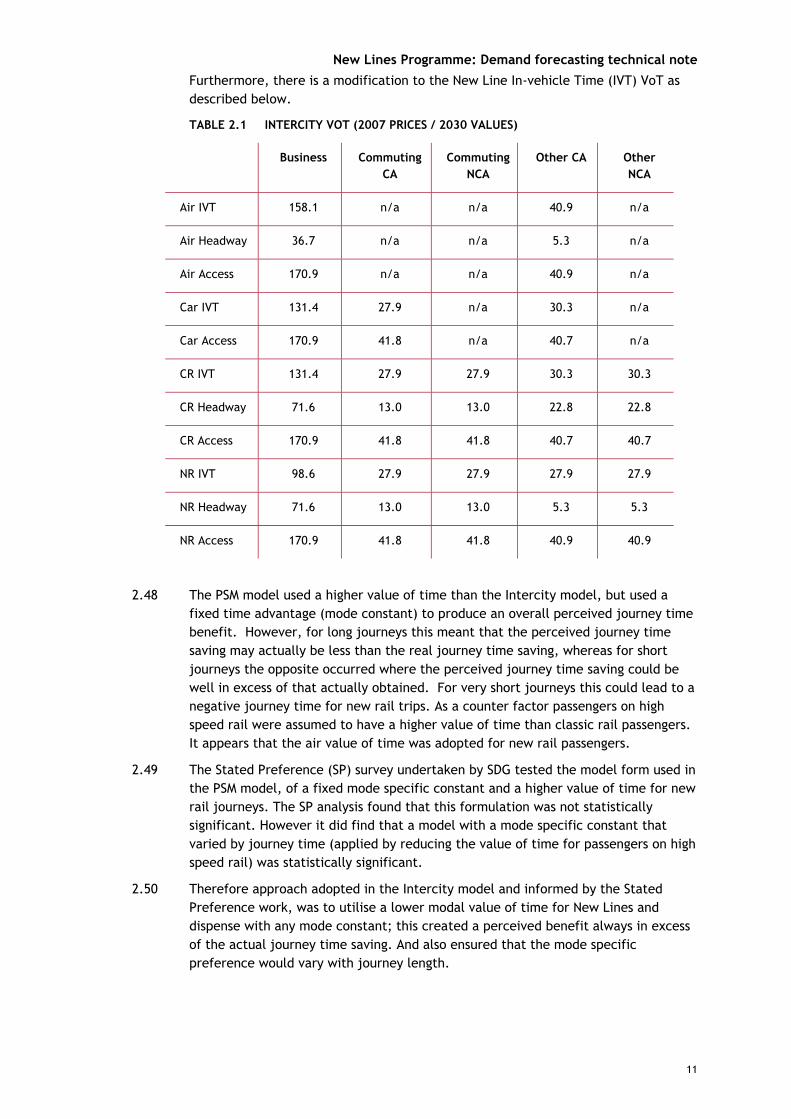
2.47 Since trunk GJTs are weighted in the Intercity model, it is necessary to ensure that the correct combination of Values of Time (VoT)s are used; these are shown in Table 2.1. PSM VoTs are taken as a starting point. These VoTs are uprated to 2030 values (the forecasting year) and modified to a 2007 price base (the forecast price base).
New Lines Programme: Demand forecasting technical note
11
Furthermore, there is a modification to the New Line In-vehicle Time (IVT) VoT as described below.
TABLE 2.1 INTERCITY VOT (2007 PRICES / 2030 VALUES)
Business Commuting CA
Commuting NCA
Other CA Other NCA
Air IVT 158.1 n/a n/a 40.9 n/a
Air Headway 36.7 n/a n/a 5.3 n/a
Air Access 170.9 n/a n/a 40.9 n/a
Car IVT 131.4 27.9 n/a 30.3 n/a
Car Access 170.9 41.8 n/a 40.7 n/a
CR IVT 131.4 27.9 27.9 30.3 30.3
CR Headway 71.6 13.0 13.0 22.8 22.8
CR Access 170.9 41.8 41.8 40.7 40.7
NR IVT 98.6 27.9 27.9 27.9 27.9
NR Headway 71.6 13.0 13.0 5.3 5.3
NR Access 170.9 41.8 41.8 40.9 40.9
2.48 The PSM model used a higher value of time than the Intercity model, but used a fixed time advantage (mode constant) to produce an overall perceived journey time benefit. However, for long journeys this meant that the perceived journey time saving may actually be less than the real journey time saving, whereas for short journeys the opposite occurred where the perceived journey time saving could be well in excess of that actually obtained. For very short journeys this could lead to a negative journey time for new rail trips. As a counter factor passengers on high speed rail were assumed to have a higher value of time than classic rail passengers. It appears that the air value of time was adopted for new rail passengers.
2.49 The Stated Preference (SP) survey undertaken by SDG tested the model form used in the PSM model, of a fixed mode specific constant and a higher value of time for new rail journeys. The SP analysis found that this formulation was not statistically significant. However it did find that a model with a mode specific constant that varied by journey time (applied by reducing the value of time for passengers on high speed rail) was statistically significant.
2.50 Therefore approach adopted in the Intercity model and informed by the Stated Preference work, was to utilise a lower modal value of time for New Lines and dispense with any mode constant; this created a perceived benefit always in excess of the actual journey time saving. And also ensured that the mode specific preference would vary with journey length.

New Lines Programme: Demand forecasting technical note
12
2.51 This is illustrated in Figure 2.2 and 2.3.for a classic rail journey of 240 minutes and 120 minutes respectively transferring to New Lines. For the former the PSM model has a lower perceived journey time where the New Line offers journey times more than 120 minutes; conversely, the approach used in the Intercity model has perceived time benefits consistently above the actual time saving. For the latter, classic rail journey of 120 minutes, the PSM model has relatively large perceived time benefits compared to the Intercity model used here.
TABLE 2.2 ILLUSTRATIVE PERCEIVED JOURNEY TIME BENEFIT FOR A 240 MINUTE CLASSIC RAIL JOURNEY SWITCHING TO NEW LINES
0
50
100
150
200
250
90 100 110 120 130 140 150 160 170 180New Line time
Tim
e be
nefit
Actual Time savingPSM Business time savingIntercity Model Business time savingPSM Lesiure time savingIntercity Model Leisure time saving

New Lines Programme: Demand forecasting technical note
13
TABLE 2.3 ILLUSTRATIVE PERCEIVED JOURNEY TIME BENEFIT FOR A 120 MINUTE
CLASSIC RAIL JOURNEY SWITCHING TO NEW LINES
2.52 Therefore on the basis of the SP results and review of the treatment of modal preference, the Intercity model adopted a factor of 75% of classic rail value of New Line value of time for Business travellers. For Leisure travellers, the ratio is 92%. Commuters are assumed to place no preference on classic rail or New Lines.
2.53 Due to two factors the SP results were not used to replace all parameters. Changing the parameters that exist in the present day would have required model recalibration. Furthermore the SP analysis produced a value of time for leisure passengers that was deemed too high and not appropriate for use.
Crowding and Network Topology
2.54 Crowding can be an important factor (and therefore an addition to the generalised cost) when someone is choosing how to travel. In order to take crowding into account, it is necessary to include a cost for it in the GJT module.
2.55 The crowding process in the Intercity model works on the New Lines mode of the model only. For a discussion on crowding assumptions and how to use the model to calculate classic rail crowding in the Do-Minimum, see paragraphs 2.94 to 2.96.
2.56 Crowding is calculated on a “link” basis. This means that for a given rail link between two Trunk Access Points the entire demand and the entire capacity over that link is used to determine the level of crowding over the link.
2.57 The network topology is used to relate the network links and the services and associated demand that run over them. This takes the form of a matrix for each link (up to 20 links are allowed). The matrix is made up of 20x20 TAP origins and destinations. For each link a flag is set if a train for any particular O to D would run over that link. By adding this information for each link the network topology is defined. This information can then be used to determine how many services run over each link. A further input defining the train stopping pattern, frequency and capacity is required. This therefore enables the total capacity on each link to be calculated.
0
20
40
60
80
100
120
140
160
30 40 50 60 70 80 90New Line time
Tim
e be
nefit
Actual Time savingPSM Business time savingIntercity Model Business time savingPSM Lesiure time savingIntercity Model Leisure time saving
New Lines Programme: Demand forecasting technical note
14
2.58 Note that there is only space for one network topology input per spreadsheet. This means that a single spreadsheet must be used for any particular network topology. It is, however, possible to add all possible links to the network topology and refer to only some of the TAPs in any given scenario.
2.59 Demand on each link is determined by totalling the demand for each OD flow that uses a particular link and a crowding cost for each link is calculated. Crowding costs are calculated on an all day basis using crowding penalty curves derived for this purpose. These curves define the crowding penalty as a proportion of the in-vehicle time; the relevant multiplier is thus applied to the journey time for each link to determine a crowding cost for that link. Note that this process infers that all services over each link are available to all of the demand; clearly there will be instances where this is not the case. Careful design of the TAP and link system can be used to mitigate this effect. This issue should not materially affect the result of the current New Line options given the service patterns modelled.
2.60 The crowding penalty is then fed back into the GJT cost for each trunk, which in turn alters the demand. A macro is used to iterate through the process up to ten times, with the resultant fed-back crowding cost being an average of previous runs to ensure that the process converges.
Valuing Crowding
2.61 The incorporation of crowding into the Intercity model required a relatively simple, robust way of estimating the impact of crowding on demand, consistent with best practice. The exact requirement was for a function to convert average load factor on each TAP to TAP link to a crowding time penalty.
2.62 The methodology used is drawn heavily from that used in the NMF and comprises two key steps:
I Establishment of crowding time penalties by load factor for an individual train based on PDFH valuations; and
I Application of distributions representing the variation of demand over an appropriate time period to give average crowding time penalties over a number of services.
Crowding Time Penalties
2.63 Whilst PDFH 4.1 expresses crowding penalties in terms of pence per minute, the NMF reflects current DfT guidance and uses an approach where the penalties are represented in terms of minutes of penalty per minute of journey time (as does the PSM model). Previous versions of the PDFH presented crowding penalties in both formats, and whilst it now only quotes monetary valuations, the time equivalent values can be derived by going back to the source studies as explained in the documentation. One of the reasons for using this approach is that it is difficult to apply the monetary approach at a link level as fares are not defined at that level. Table 2.4 details the resulting table of crowding penalties.

New Lines Programme: Demand forecasting technical note
15
TABLE 2.4 IMPLIED JOURNEY TIME EQUIVALENT CROWDING PENALTIES
Standard First Class Outer Inner60% - - - - - - - - 70% 0.04 0.04 - - - 0.02 0.04 - 80% 0.07 0.08 - - - 0.04 0.08 - 90% 0.15 0.16 0.23 0.04 - 0.07 0.11 0.11
100% 0.20 0.23 0.47 0.07 0.08 0.09 0.15 0.22 110% 0.27 0.31 0.11 0.16 0.15 0.21 0.32 120% 0.33 0.39 0.14 0.23 0.22 0.27 0.43 130% 0.40 0.46 0.18 0.31 0.28 0.34 0.54 140% 0.45 0.54 0.22 0.39 0.35 0.40 0.65 150% 0.47 160% 0.55
Standard First Class Outer InnerBelow 100% 0 - - - - - -
100% 2.12 1.70 1.28 1.28 2.12 2.86 1.76 110% 2.33 1.87 1.33 1.33 2.33 2.93 1.89 120% 2.54 2.04 1.38 1.38 2.54 3.01 2.03 130% 2.75 2.21 1.44 1.44 2.75 3.08 2.16 140% 2.96 2.38 1.49 1.49 2.96 3.15 2.30 150% 1.54 1.54 2.43 160% 1.60 1.60 2.57
Standing Penalties (time penalties)
Load Factor
London-based Services Non-London Based Services
Leisure Business Commuting
Leisure Business Commuting
Load Factor
London-based Services Non-London Based Services
Leisure Business Commuting
Leisure Business Commuting
Sitting Penalties (time penalties)
2.64 These were simplified to a set of recommended values for a single train service, which has been reduced to penalties for Commuting (split London and non-London based) and non-Commuting. This simplification reflects uncertainty in the original valuations, the need for internal consistency and consistency with the standard GJT approach.
2.65 The penalties shown in Table 2.5 were adopted for use in NMF, and have been adopted for this work. The penalties are applied to in-vehicle times at the load factors shown and are additional to actual journey time. Values at 300% load factors are derived by extrapolation from the values at 120% and 140%.

New Lines Programme: Demand forecasting technical note
16
TABLE 2.5 PROPOSED TIME EQUIVALENCE PENALTIES – INDIVIDUAL TRAIN
Load Factor Condition London-Based
Commuting1
Non- London
Commuting2
Non-Commuting3
60% and below
Sitting -
- -
80% Sitting - 0.07 0.07
90% Sitting 0.02 0.12 0.12
100% Sitting 0.08 0.17 0.17
120% Sitting 0.19 0.30 0.30
140% Sitting 0.30 0.43 0.43
300% Sitting 1.18 1.47 1.47
Below 100% Standing - - -
100% Standing 1.28 1.76 2.20
120% Standing 1.38 2.03 2.53
140% Standing 1.49 2.30 2.86
300% Standing 2.37 4.46 5.50
Using a Distribution to Estimate Average Crowding Costs for a Link
2.66 Load factors are available for each link within the model. In general this means that the resulting load factors will be averages over a number of train services over an average day.
2.67 The consequence of this is that, if there is any variability in load factors across services, then crowding off will start at an average load factor of less than the 80% shown in Table 2.5. This is because there will be some trains with higher load factors than the average, which incur crowding penalties, and this is not offset by those trains at lower load factors than the average which have zero crowding penalties. In general, crowding penalties for average load factors will be higher than for individual trains with the same load factor because of this asymmetry.
2.68 The construction of crowding curves assumes that distributions of load factors can be modelled using a Gamma distribution with an assumed distribution between the standard deviation and mean load factor. The ratio of the standard deviation to the mean load factor is assumed to remain constant as the mean load factor varies.
1 Arithmetic average of London based Commuting Outer and Inner from Table 2.4 2 Standing penalties as per Non-London based Commuting services, sitting penalties constrained to non-
Commuting values from Table 2.4 3 Arithmetic average of London based Leisure and Standard Business and Non-London based Leisure and
Business values from Table 2.4
New Lines Programme: Demand forecasting technical note
17
2.69 The Gamma distribution form is used because it approximates to a Normal distribution for certain parameter values, except that it is (usefully) non-negative. These distributions allowed us to infer a revised table of crowding penalties based on average load factors.
2.70 The NMF employed a process for fitting Gamma distributions for individual TOCs and time periods and this been adopted for application in the New Lines study, using the distribution parameters from the most appropriate TOCs for the whole day, rather than individual time period, derived by returning to the raw data.
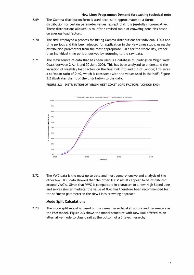
2.71 The main source of data that has been used is a database of loadings on Virgin West Coast between 2 April and 30 June 2006. This has been analysed to understand the variation of weekday load factors on the final link into and out of London; this gives a sd/mean ratio of 0.40, which is consistent with the values used in the NMF. Figure 2.2 illustrates the fit of the distribution to the data.
FIGURE 2.2 DISTRIBUTION OF VIRGIN WEST COAST LOAD FACTORS (LONDON END)
2.72 The VWC data is the most up to date and most comprehensive and analysis of the other NMF TOC data showed that the other TOCs’ results appear to be distributed around VWC’s. Given that VWC is comparable in character to a new High Speed Line and serves similar markets, the value of 0.40 has therefore been recommended for the sd/mean parameter in the New Lines crowding approach.
Mode Split Calculations
2.73 The mode split model is based on the same hierarchical structure and parameters as the PSM model. Figure 2.3 shows the model structure with New Rail offered as an alternative mode to classic rail at the bottom of a 3 level hierarchy.
0%
10%
20%
30%
40%
50%
60%
70%
80%
90%
100%
0.000 0.500 1.000 1.500
Load factor
% o
f dis
trib
utio
n le
ss th
an lo
ad fa
ctor
All weekday flows starting or ending in London Analytically derived distribution

New Lines Programme: Demand forecasting technical note
18
FIGURE 2.3 HIERACHICAL LOGIT MODEL STRUCTURE
2.74 After classic rail, new rail, air and car generalised costs have been calculated, these costs are used to calculate estimates of the future modal share between the four modes. This is achieved using an incremental nested, or hierarchical, logit model, which is a statistical model commonly used to forecast the choices made by people faced with a series of discrete options. The inputs to the model are the Do-Minimum modal share and both Do-Minimum and Do-Something generalised costs, along with a number of parameters that influence how sensitive the model is to differences in the generalised costs. The output of the model is a number of conditional probabilities, which are interpreted as being the percentage of travellers choosing each mode when faced with the choice.
2.75 At the top of the nest, costs are aggregated to reflect the overall improvement in transport and this is used to obtain an estimate of generated demand.
Parameters
2.76 The PSM mode choice and generation scaling parameters were employed, but modified to take account of the change in the modelled price base. The PSM model has a base year of 2000 and all monetary values are expressed in a price base of that year; the Intercity model has an equivalent (price) base year of 2007. This esults in, all other things being equal, a bigger monetary cost since the price base is higher. On that basis, the scaling parameters are reduced in compensation. RPI data for 2000 and 2007 was used to inflate values of time, with a corresponding reduction in the scaling parameters. The resulting scaling parameters are set out in Table 2.6.
All modes
‘PT’ modes
Rail modes
Classic Rail
New Rail Air Car

New Lines Programme: Demand forecasting technical note
19
TABLE 2.6 SCALING FACTORS
Scaling factor λ Business Commuting (CA)
Commuting (NCA)
Other (CA)
Other (NCA)
Classic rail versus new rail -0.000630 -0.000961 -0.000951 -0.002679 -0.004146
Rail versus air -0.000561 -0.001855
Public transport versus car -0.000409 -0.000666 -0.000981
Generation -0.000061 -0.000222 -0.000222 -0.000327 -0.000327
2.77 The generation scaling parameters are based on a factor (thetas strictly speaking – ratios of scaling parameters) applied to the scaling parameter of the public transport versus car top nest. The default PSM value is 1/3 for all purposes, but this was reduced for Business to 0.15, based on review and analysis of model results and comparison and benchmarking against modelled and empirical results obtained elsewhere. It must be noted that the value of the generation scaling parameters (and hence the factor or theta applied) is a critical parameter and has a very large influence on the level of demand on New Lines. The values chosen are considered to give plausible forecasts, consistent with other forecasting methodologies and benchmarking.
Application of the Mode Choice Model
2.78 The model was applied on an O-D basis and comprises five main steps. In all cases, where New Lines is identified as not competing with classic rail on a particular flow, the Do-Minimum mode split and demand is taken as the default result. Since crowding is modelled, the following process is done on an iterative process, with ten iterations being undertaken and a dampening process implemented to force convergence.
Step 1: Classic Rail versus New Rail mode choice
2.79 This stage models the choice between classic rail and new rail. At this stage the model operates on an absolute basis for the Do-Something (i.e. with new rail) scenario only, since new rail does not exist in the Do-Minimum scenario and there is therefore no mode choice to be made.
2.80 Generalised costs are fed into the model in units of pence and modal share is calculated using the formulae:
( )CR
NR
)railNRP( GCλGCλ
GCλ
ANRA
A
eee
⋅−⋅−
⋅−
+= and ( )CRNR
CR
)railCRP( GCλGCλ
GCλ
AA
A
eee
⋅−⋅−
⋅−
+=
where λ is the scaling factor and GCNR and GCCR are the generalised costs of new rail and classic rail respectively.

New Lines Programme: Demand forecasting technical note
20
2.81 Composite costs for the rail mode were calculated using the formula,
)ln(1CRNR
railGCλGCλ
A
AA eeλ
GC ⋅−⋅− +−=
2.82 The change in composite cost between the Do-Minimum and Do-Something was calculated as,
CRrailrailΔ GCGCGC −=
Step 2: Rail versus air mode choice
2.83 At this stage the change in cost calculated in the lower nest is compared with the generalised cost of air travel, using the incremental logit formula,
( )airrail
rail
airrail
rail)PTRailP( GCλGCλ
GCλ
BB
B
ePePeP
Δ⋅−Δ⋅−
Δ⋅−
+=
and
( )airrail
air
airrail
air)PTAirP( GCλGCλ
GCλP
BB
B
ePePe
Δ⋅−Δ⋅−
Δ⋅−
+=
where Pair and Prail are the Do-Minimum percentage mode share of the air and rail modes respectively .
2.84 Composite costs are again calculated and fed to the public transport vs car mode choice model. The formula used is
)ln(1railair
railairPTGCλGCλ
B
BB ePePλ
GC Δ⋅−Δ⋅− +−=Δ
2.85 If no Do-Minimum air demand exists for a flow, rail is assumed to capture 100% of the modal share and the rail composite cost is fed directly to the next nest in the model hierarchy.
Step 3: Public transport versus car mode choice
2.86 The change in cost calculated in the preceding nest is compared with the generalised cost of car travel. The same incremental logit formulae are used as in the preceding level, with different costs and parameters as appropriate. Composite costs are again calculated and used to calculate generated demand.
Step 4: Generated demand
2.87 With composite costs calculated at the top nest in the model structure, the generated demand is calculated, with Do-Something demand equating to:
all31
DMDS
GCλCeDDΔ⋅−
=
Step 5: Do-Something demand
2.88 In the final stage the generated demand is added to the Do-Minimum demand and the total figure is apportioned using the probabilities calculated at each stage in the mode choice model.
2.89 For a number of flows the difference in GJT between NR and CR is fairly large. This is particularly true of flows with large access times to a NR TAP. The NR mode share parameter can be set to ensure that demand from flows with mode share less than

New Lines Programme: Demand forecasting technical note
21
the parameter threshold is not assigned to New Rail. This ensures that material revenue generated from lots of small revenue gains is not claimed.
Running the Model
2.90 The model needs Do-Minimum costs for classic rail, air and car and Do-Something costs for classic rail, new rail, air and car. Usually when running the model, car and air costs are unchanged from Do-Minimum to Do-Something.
2.91 The model is designed to be able to store and run multiple, but broadly similar, Do-Something scenarios (where a scenario is a set of fares, journey times and service intervals). Each scenario can be run simply by switching the scenario selector in the parameter sheet and rerunning the crowding process.
2.92 However, since the mode choice between new rail and classic rail will only be calculated if the relevant new rail flow is also in scope in the Do-Minimum, it is important to ensure that every scenario run is tested against the relevant Do-Minimum costs. This means that the correct set of Do-Minimum costs must be input into the model and that separate versions of the model will be needed when different sets of Do-Minimum costs are needed (for example when testing options that serve different corridors).
2.93 Furthermore, it is important to note that crowding costs must be calculated for both the Do-Minimum classic rail and the Do-Something new rail costs. It is assumed that there is no crowding on classic rail flows where a New Line flow is introduced on the basis that the majority of the flow will transfer to New Rail, with most flows on the classic network not being subject to crowding (since for example travellers will have used the classic network in order to minimise the fare and hence used advanced booking with a seat). To keep the model size operable, the crowding function is only applicable to the New Rail GJTs and therefore to run crowding on CR in the Do-Minimum, a separate model is used and the CR Do-Minimum scenario run through the NR flow, including the crowding process.
Do-Minimum
2.94 The process for running the CR DM is described below:
I Set up Air information (TAPs, access radii, journey time, service interval and fares)
I Set up CR information (TAPs, access radii, journey time, service interval and fares) in the NR inputs
I Set up the network topology – this will included as many major TAPs as needed to ensure a realistic demand on trains to ensure crowding is correctly calculated
I Set up train service spec to determine train capacity for crowding
I Switch “Use GJT weighting” to “NO”. This ensures that the NR JT weighting is switched off (to ensure that CR GJTs are calculated). Also changing the switch forces the given demand results to be the results of the crowding process (rather than the outputs of the mode split model).
I Set up other parameters
I Clear then run the crowding macro

New Lines Programme: Demand forecasting technical note
22
I The figures in the sheet “DM Results for DS” can then be copied to the DS version of the model into the “DM Results Inputs” sheet.
2.95 It is important to check that the right zones are in scope for all TAPs. It might be necessary to modify the IVT manual adjustment parameters to allow certain zones to be assigned as in-scope.
2.96 To ensure correct working of the mode split model, the CR DM should include feasible journeys that are expected to be in scope in the NR DS. This is to ensure there is a competitive CR option for the model split mode to perform its calculations on.
Do-Something
2.97 The process for running the DS is described below:
I Ensure correct DM results have been copied into the “DM Results Inputs” sheet
I Set up Air information (typically unchanged from DM)
I Input NR TAPs and access radii into NR TAP definition
I Input fares, service interval and JT into NR inputs
I Set up Classic rail DS into CR inputs. The same TAPs and access radii must be used as in the DM. Fares, service interval and journey times can be modified.
I Set up NR network topology – this would be point–point links for high speed non-stop rail service
I Set up train service specification to determine train capacity for crowding
I Ensure Switch “Use GJT weighting” is “YES”
I Set up other parameters
I Run crowding
I Further NR scenarios can be run by selecting the relevant scenario in the “GJT Parameters” sheet.
2.98 This process is outlined in the “Model Flow” sheet in the model.
Model Outputs
2.99 A number of model outputs are available to the user. These are described below.
Appraisal Results
2.100 As well as the demand and revenue results, the model produces outputs for appraisal related information such as journey time savings per mode and crowding and fares benefits and disbenefits. These benefits are derived from the calculated logsum results for New Rail vs Classic Rail nest in the mode split model and the results for the air and car directly. The detail of these calculations is discussed in the appraisal document.
Top 30 & Summary
2.101 The summary sheet displays the demand, revenue and passenger miles for the relevant link selected (in the Top 30 sheet). The Top 30 results sheet lists the 30 largest individual flows that make up the results in the summary sheet. This list is

New Lines Programme: Demand forecasting technical note
23
generated using a macro. This is a useful way of determining which flows are in scope for a TAP-TAP link.
2.102 Flows with no demand are not shown here but as there may be some zones in scope with no demand, users can use the autofilters on the “Re-map demand” sheet to search for all zones in scope (irrespective of demand).
Single Flow Debug
2.103 A single flow can be studied using the spreadsheet to look at how demand GJT changes, how demand reacts to that and also what components make up the GJT. This can be very useful for debugging the mode choice decisions made by users on the edges of high speed catchments.
Illustrative Model Results
Scenario Setup
2.104 In this section, the results of a model run for an example scenario are presented. Option MB1.4.1 (shown in) is run through version 3.0 of the Intercity model. The following assumptions are made for key parameters:
I VoT inputs are as described in Table 2.1;
I No MSC;
I Scaling parameters and generation factors as set out in Table 2.6;
I Fares from NMF (converted to 2007 price base);
I 30% premium on NR fares; and
I 66 mins 4tph London to Manchester, 129 mins 2 tph London to Edinburgh.

New Lines Programme: Demand forecasting technical note
24
FIGURE 2.4 OPTION MB1.4.1
EdinburghGlasgow
Liverpool
Birmingham
Manchester
London Central
Preston
WM South Junc.
GM North Junction
WM West Junc.
GM South Junc.
WM North Junc.Mersey Junction
Caledonian Junc
Warrington
Form ation 10 10 10 10 10 10 10 10 10 10 10 10 10 10 5 5 5 5
Glasg ow
Edinburgh
Preston
Liverpool
Warrington
Manchester
Birm ingham
London1 2 3 4 5 6 7 8 9 10 11 12 13 14 15 16 17 18
Option M B 1.4.1 (TPH )
Do-Minimum
2.105 A full DM network of 20 TAPs is defined and feasible journey times and costs are input. Additionally, a network of links is defined to enable train crowding calculations.
2.106 Figure 2.5 and Figure 2.6 respectively show the zones in catchment for London and Manchester/Stockport in the Classic Rail Do-Minimum scenario. For London the catchment radius is set to 90 minutes (GJT) and for Manchester it is 60 minutes (GJT). Both stations are allowed rail access only to reflect the difficulty of access by car. Note that the catchments do not change depending on the flow being served.
2.107 For London, the catchment has been manually adjusted to include South Coast zones since anyone travelling from these zones by rail must access services to the North via a London station. Manchester has a reasonably small catchment compared to London since other nearby TAPs are specified such as Liverpool, Warrington and Leeds.

New Lines Programme: Demand forecasting technical note
25
FIGURE 2.5 LONDON DO-MINIMUM CATCHMENT
FIGURE 2.6 MANCHESTER DO-MINIMUM (CLASSIC RAIL) CATCHMENT

New Lines Programme: Demand forecasting technical note
26
2.108 The crowding levels that are generated are shown in Table 2.7. Pendolino WCML trains are assumed to have 577 seats and the ECML IEP Intercity is assumed to have 639. Of note, the load factor on the Birmingham services peak at 59% out of London, with the equivalent load factor for Manchester services peaking at 44%. The highest load factor occurs on the Glasgow service, with high volumes and crowding to Warrington and beyond.
TABLE 2.7 DO-MINIMUM CROWDING LEVELS
Link TAP - TAP journey Demand Capacity Load FactorJourney
TimeCrowding Cost
(Comm)Crowding Cost (Non-Comm)
per day per day mins mins minsA London Central to Coventry 32,721 55,392 59% 63 2.6 6.0B Coventry to Birmingham Central 28,236 55,392 51% 20 0.3 0.9C Birmingham Central to Wolverhampton 1,919 18,464 10% 24 0.0 0.0D London Central to Stafford 9,264 18,464 50% 81 1.1 3.2E Stafford to Liverpool Central 8,550 18,464 46% 46 0.3 1.1F London Central to Warrington 16,360 27,696 59% 108 4.4 10.2G Warrington to Wigan 14,539 18,464 79% 11 1.9 3.6H Wigan to Preston 12,708 18,464 69% 13 1.2 2.5I Preston to Lancaster 6,956 18,464 38% 18 0.0 0.1J Lancaster to Oxenholme 6,028 18,464 33% 15 0.0 0.0K Oxenholme to Carlisle 4,702 18,464 25% 36 0.0 0.0L Carlisle to Glasgow 3,938 18,464 21% 71 0.0 0.0M London Central to Stockport 24,426 55,392 44% 119 0.6 2.2N Stockport to Manchester 16,216 55,392 29% 7 0.0 0.0O London Central to Leeds 18,813 40,896 46% 116 0.8 2.9P London Central to York 25,940 61,344 42% 118 0.4 1.7Q York to Newcastle 17,073 40,896 42% 50 0.2 0.7R Manchester to Preston 2,439 14,400 17% 48 0.0 0.0S Newcastle to Edinburgh 7,447 20,448 36% 84 0.1 0.4T Wolverhampton to Stockport 2,928 9,600 31% 65 0.0 0.1
Do-Something
2.109 As illustrated in Figure 2.7, the Manchester catchment increases significantly to reflect the fact that people are willing to travel further to access New Lines because of the reduced trunk journey time. The catchment area for London does not change.
FIGURE 2.7 MANCHESTER DO-SOMETHING (NEW LINES) CATCHMENT

New Lines Programme: Demand forecasting technical note
27
2.110 New Line crowding is shown in Table 2.8. The capacities of the trains are assumed to be 650 seats. Note that the London to Glasgow demand is shown on the London to Preston and Preston to Glasgow links. The highest load factors are shown on the Scottish services, with the Birmingham and Manchester all day load factors being lower than the Do-Minimum at 32% and 42% respectively.
TABLE 2.8 NEW LINE CROWDING
Link TAP - TAP journey Demand Capacity Load FactorJourney
TimeCrowding Cost
(Comm)Crowding Cost (Non-Comm)
per day per day mins mins minsA London Central to Birmingham Central 26,915 83,200 32% 46.0 0.0 0.1B London Central to Manchester Central 34,986 83,200 42% 66.0 0.2 0.9C Birmingham Central to Manchester Central 6,689 41,600 16% 38.0 0.0 0.0D London Central to Warrington 20,000 41,600 48% 66.0 0.7 2.1E Liverpool Central to Warrington 12,148 41,600 29% 15.0 0.0 0.0F London Central to Preston 23,504 41,600 57% 73.0 2.4 5.8G London Central to Glasgow 0 0 0% 136.0 0.0 0.0H London Central to Edinburgh 21,528 41,600 52% 129.0 2.4 6.4I Manchester Central to Preston 7,295 20,800 35% 15.0 0.0 0.1J Preston to Glasgow 18,565 62,400 30% 59.0 0.0 0.1K Preston to Edinburgh 2,555 20,800 12% 59.0 0.0 0.0L Birmingham Central to Preston 2,577 41,600 6% 46.0 0.0 0.0M 0 0 0% 0.0 0.0 0.0N 0 0 0% 0.0 0.0 0.0O 0 0 0% 0.0 0.0 0.0P 0 0 0% 0.0 0.0 0.0Q 0 0 0% 0.0 0.0 0.0R 0 0 0% 0.0 0.0 0.0S 0 0 0% 0.0 0.0 0.0T 0 0 0% 0.0 0.0 0.0
Results Summary
2.111 The summary in Table 2.9 shows that demand on the London - Manchester new line trunk is 10.50m journeys per year of which 7.13m of these journeys are abstracted from Classic rail. It is important to understand that the total classic rail journeys figure shown is not the number of journeys made on the London to Manchester classic rail trunk. It is the number of classic rail journeys that are made between the same set of origins and destinations that are in scope for the new line. For example Classic Rail journeys between Leeds and London are included since a small proportion of these passengers may choose to travel to London via the New Line from Manchester due to the high speed of the service offered between London and Manchester.
TABLE 2.9 LONDON-MANCHESTER JOURNEYS RESULTS SUMMARY
CR NR Air Car TotalDM mill jnys /year 12.10 0.00 0.40 3.84 16.34DS mill jnys /year 4.97 10.50 0.20 3.07 18.74
Difference mill jnys /year -7.13 10.50 -0.20 -0.76 2.40% Difference -59% -51% -20% 15%
2.112 The breakdown of the Top 30 value (by revenue) zone pairs on the Manchester corridor is shown in Table 2.10
2.113 Looking more closely at a single flow (Table 2.11), in this case London to Stockport Business travellers, the results of the mode choice calculations is visible. For London to Stockport there is a significant GJT benefit from travelling via New rail and 91% of the existing classic rail passengers shift. As well as mode shift from air and car, there is generation of 713 passengers per day on this flow.

New Lines Programme: Demand forecasting technical note
28
TABLE 2.10 TOP 30 FLOWS LONDON – MANCHESTER
2030 Do Minimum 2030 Do SomethingCR Air Car CR NR Air Car
Flow Zone 1 Zone 2 Demand Revenue Yield Demand Demand Demand Revenue Yield Demand Revenue Yield Demand Demandm jnys /
year £m / year £/jnym jnys /
yearm jnys /
yearm jnys /
year £m / year £/jnym jnys /
year £m / year £/jnym jnys /
yearm jnys /
year1 117_130 London Central Manchester 4.0 195.5 49.1 0.0 0.2 0.2 9.5 47.3 5.1 331.8 64.5 0.0 0.12 117_187 London Central Stockport 1.9 140.8 74.8 0.0 0.1 0.1 9.4 78.0 2.3 153.1 65.7 0.0 0.03 117_125 London Central Macclesfield 0.4 27.6 78.0 0.0 0.0 0.0 0.7 81.2 0.6 38.5 68.5 0.0 0.04 117_210 London Central Tameside 0.3 17.7 50.8 0.0 0.0 0.0 0.9 48.9 0.5 30.9 66.1 0.0 0.05 105_117 Leeds London Central 4.4 239.1 54.7 0.0 0.2 4.2 228.1 54.5 0.3 20.6 78.5 0.0 0.16 100_117 Kirklees London Central 0.2 13.8 56.9 0.0 0.1 0.1 3.2 55.9 0.3 20.4 70.4 0.0 0.07 17_130 Brighton & Hove Manchester 0.1 7.3 62.7 0.0 0.1 0.0 0.4 59.7 0.2 14.4 77.6 0.0 0.08 118_130 London North Manchester 0.1 4.5 53.8 0.0 0.1 0.0 0.2 52.2 0.2 11.0 70.1 0.0 0.09 9_117 Bolton London Central 0.1 3.0 50.6 0.0 0.0 0.0 0.2 49.6 0.1 7.2 67.1 0.0 0.0
10 117_157 London Central Oldham 0.1 3.1 50.7 0.0 0.0 0.0 0.2 49.5 0.1 6.9 67.0 0.0 0.011 123_130 London West Manchester 0.0 1.3 53.0 0.0 0.1 0.0 0.1 52.3 0.1 5.9 70.3 0.0 0.012 104_130 Kent West Manchester 0.0 0.9 58.9 0.0 0.1 0.0 0.1 58.3 0.1 4.1 76.3 0.0 0.113 124_130 Luton Manchester 0.0 0.7 61.0 0.0 0.2 0.0 0.1 59.9 0.0 3.7 78.0 0.0 0.214 93_130 Hertfordshire Mml Manchester 0.0 1.5 56.6 0.0 0.0 0.0 0.1 54.4 0.0 3.6 72.3 0.0 0.015 122_130 London South West Manchester 0.0 0.6 51.5 0.0 0.1 0.0 0.1 51.7 0.1 3.5 69.8 0.0 0.016 92_130 Hertfordshire Ecml Manchester 0.0 0.6 54.2 0.0 0.2 0.0 0.1 54.6 0.0 3.1 72.6 0.0 0.117 17_210 Brighton & Hove Tameside 0.0 0.7 63.6 0.0 0.1 0.0 0.1 62.1 0.0 2.8 80.0 0.0 0.018 71_130 Essex South Manchester 0.0 0.5 57.1 0.0 0.2 0.0 0.1 57.2 0.0 2.6 75.2 0.0 0.119 130_208 Manchester Surrey North West 0.0 0.4 55.8 0.0 0.0 0.0 0.1 55.1 0.0 2.4 73.4 0.0 0.020 130_207 Manchester Surrey East 0.0 0.5 55.0 0.0 0.0 0.0 0.1 54.5 0.0 2.4 72.6 0.0 0.021 130_209 Manchester Surrey South West 0.0 0.8 56.7 0.0 0.0 0.0 0.1 55.7 0.0 2.3 73.6 0.0 0.022 120_130 London South / Croydon Manchester 0.0 0.6 52.0 0.0 0.0 0.0 0.1 51.3 0.0 2.2 69.2 0.0 0.023 121_130 London South East Manchester 0.0 0.4 51.9 0.0 0.0 0.0 0.0 52.3 0.0 1.9 70.2 0.0 0.024 17_187 Brighton & Hove Stockport 0.0 0.8 87.1 0.0 0.0 0.0 0.1 89.1 0.0 1.7 77.8 0.0 0.025 100_118 Kirklees London North 0.0 0.8 59.5 0.0 0.0 0.0 0.2 59.3 0.0 1.6 74.2 0.0 0.026 69_130 East Sussex Manchester 0.0 0.3 59.8 0.0 0.0 0.0 0.0 59.2 0.0 1.5 77.2 0.0 0.027 117_170 London Central Rochdale 0.0 0.3 50.7 0.0 0.0 0.0 0.0 50.9 0.0 1.4 68.9 0.0 0.028 13_130 Bedfordshire North Manchester 0.0 0.2 60.1 0.0 0.0 0.0 0.0 59.4 0.0 1.2 77.4 0.0 0.029 130_225 Manchester West Sussex Central 0.0 0.3 58.8 0.0 0.0 0.0 0.0 56.8 0.0 1.0 74.7 0.0 0.030 103_130 Kent East Manchester 0.0 0.3 60.6 0.0 0.0 0.0 0.0 59.0 0.0 0.9 76.8 0.0 0.0
Total 11.71 665.0 56.8 0.27 1.9 4.63 254.2 54.9 10.29 684.6 66.6 0.10 1.26

New Lines Programme: Demand forecasting technical note
29
TABLE 2.11 LONDON - STOCKPORT DETAIL
117_187 Business CAper day CR NR Air Car Total
DM GJT mins 246 0 260 210DS GJT mins 260 207 260 210% Diff GJT 6% N/A 0% 0%DM Dmd jnys 3395 0 28 146 3569DS Dmd jnys 316 3908 6 52 4282Diff Dmd jnys -3079 3908 -22 -94 713% Diff Dmd -91% N/A -78% -64% 20%DM Rev £ 274,406 0 274,406DS Rev £ 25,543 278,869 304,413Diff Rev £ -248,863 278,869 30,006% Diff Rev -91% N/A 11%
GJT Calculations
2.114 Figure 2.8 shows how GJT is built up for the London to Stockport flow for New Rail for business travellers. The large reduction in journey time is the key part of the NR GJT reduction. This is offset by an increased access time since users must travel to Manchester rather than catching the train from Stockport. The difference in fares is largely immaterial to business users, who value time highly.
FIGURE 2.8 DO SOMETHING GJT BREAKDOWN
DS GJT breakdown
0
50
100
150
200
250
300
CR NR Air Car
min
s
OtherConstantAccess FareAccess TimeHeadwayTrunk FareTrunk Time
Totals
2.115 For this example option, the total revenue increment from DM (shown in Table 2.12) to DS is £1.53bn. This number will drive the business case, along with the associated journey time, crowding and fare benefits.
TABLE 2.12 TOTAL REVENUE FOR OPTION 1.4.1
CR NR TotalDM £m / year 1,654 0 1,654DS £m / year 534 2,653 3,187Diff £m / year -1,120 2,653 1,533
% Diff -68% 93%

New Lines Programme: Demand forecasting technical note
30
Model Discussion
Experience of High Speed Rail
2.116 A review has been undertaken of the available literature on international experience of the introduction of high speed rail. This indicates that the introduction of high speed rail can lead to significant increases in rail demand. For example when air passengers transferring to other flights are excluded Eurostar services are estimated to carry 80% of the London to Paris market.
2.117 Journey time elasticities implied by observed changes in behaviour have been utilised to benchmark the New Line forecasts. The best available data existing relates to the initial stage of the Paris to Lyon line; this reduced train journey times by around 30% and had an implied JT elasticity of around -1.6. The second southern section stage reduced JTs by 25% but only saw a JT elasticity of -1.1. This is lower since significant transfer from air had been largely completed in stage one.
2.118 These values have been compared to the journey time elasticities implied by the New Line forecasts of circa -0.4 for Birmingham to London, -0.8 between Manchester and London and -1.54 for Edinburgh to London where there is the most to be gained from air competition. Of note, the Edinburgh elasticity is very comparable to the Paris-Lyon experience and again provides comfort that the New Lines forecasts are credible and robust.
2.119 Other evidence supports this. In a 1992 stated preference study considering air and rail travel in the UK Wardman et al found a rail journey time elasticity between –1.2 and –1.5 depending upon the size of the journey time change. Bhat (1995) reports a rail in-vehicle time elasticity of -1.56 from a study of air, rail and car competition in Canada.
2.120 There is mixed evidence on the amount of traffic that would be generated by a new high speed rail service. Wilken (2000) reports that surveys of AVE passengers indicated that 15% of the additional rail traffic was newly generated. However Bonnafous (1987) found that 49% of the additional traffic on Paris Lyons in the first four years was generated traffic.
2.121 As part of the New Lines project only a small scale review of the publicly available evidence on the impact of New Lines has been undertaken. At the next stage of the project a more significant workstream investigating the experience of existing high speed rail services should be undertaken.
UK demand flows
2.122 Forecast New Line demand for particular flows have also been compared to that achieved by existing and forecast UK flows. In particular, in option MB1.4.1 the market between Edinburgh and London is forecast to grow to 6.5m passengers per annum. The New Line journey time between Scotland and London is broadly equivalent to that from Manchester and Leeds to London today; service frequencies are comparable at 2tph or 3tph. Their Do-Minimum demand is forecast to reach 6.8
4 This is the average with and without any fare premia, the elasticity values being 1.46 and 1.62 respectively. This reflects the uncertainty around fare changes on the Paris-Lyon route on which the elasticity is being compared.

New Lines Programme: Demand forecasting technical note
31
million and 5.6 million respectively by 2030, so the demand forecasts for Edinburgh are commensurate given the rail journey times.
2.123 This is set against the relative sizes of the population. Manchester is forecast5 by 2030 to have a population some 75% greater than SE Scotland (the area served by a New Lines service to Edinburgh), with West Yorkshire (the Leeds area conurbation) some 55% greater. However, these areas are much more accessible, with road and rail offering reasonable accessibility. Conversely, only air arguably offers the same for Scotland (where rail is well over 4 hours and car has journey times of 7 hours or more).
2.124 Were accessibility levels comparable, then it can be argued that the demand for travel would be comparable, after accounting for the relative attractiveness of the markets. This is illustrated in Table 5.6 for the South East to North West and South East to Scotland markets. The attractiveness is measured by the relative level of population and employment in the two markets (the South East is common to both and hence does not affect the relative attractiveness); overall, the North West has 40% higher population and employment than Scotland in 2030.
2.125 In 2030, the Do-Minimum demand to the North West is 40 million trips per annum. Whilst the attractiveness of Scotland is some 30% lower, the demand to Scotland is nearly 50% lower, reflecting the relatively poor accessibility to Scotland from the South East. New Lines improves rail accessibility to Scotland to a level equivalent to that currently experienced for the North West; the forecasts indicate that the Scottish market grows to a size commensurate with the North West accounting for the differences in population and employment (i.e. 40/28 = 1.4).
TABLE 2.13 RELATIVE MARKET SIZE FOR THE NORTH WEST AND SCOTLAND IN 2030
South East6 to: 2030 attractiveness index (population and employment)
2030 Do-Minimum (million journeys
p.a.)
2030 Do-Something (million journeys
p.a.)
North West 1.4 40 n/a
Scotland 1 21 28
Summary
2.126 The preceding discussion has set out a set of benchmarking analysis to demonstrate the credibility and robustness of the New Lines forecasts. The forecasts are consistent with PDFH, the industry standard rail demand forecasting tool, commensurate with experience elsewhere and accord with comparison of demand on other key rail flows.
2.127 However, it must be emphasised that any forecasting is prone to uncertainty and that should the case for New Lines be considered further, the forecasting process should be developed in more detail, notably with regard the preference for New
5 TEMPRO 5.4.
6 Government Office Regions of London, South East and East of England.

New Lines Programme: Demand forecasting technical note
32
Lines over other modes and the propensity for New Lines to generate demand. Other refinements for consideration are set out below.
Potential Model Refinements
2.128 The key model refinement would be to update the demand data from the original 2000 base data. Although this was undertaken here to a new 2007 base, a more thorough update could be done using observed data, in particular for the air and rail data where good data sources exist (the CAA passenger survey and ticket sales data respectively). Updating road data should also be considered, although the source for such data is not clear and would need to be investigated.
2.129 Associated with any updates to base demand data, forecast 2030 demand could also be refined by obtaining more detailed data from the DfT forecasts. Use of the NMF data for rail is robust, but the air and highway forecasts could be done at a more disaggregate level.
2.130 It would also be helpful to have a greater understanding of the evidence and analysis underlying the original Planet Strategic model formulation.
2.131 The analysis would also benefit from greater spatial disaggregation and network based analysis, particularly in London and the South East, where access to the respective modal networks (classic rail and New Lines stations, and airports) can have a material influence on mode and route choice.
2.132 The increased catchment of the New Line may lead to an increase in the number / length of car trips to access rail services. This has not been explicitly taken into account.
2.133 Model structures and functionality could also be refined, to better capture the impacts of New Lines on trip patterns and land use impacts. This should also include updated model calibration to ensure current behavioural patterns are captured in the modelling process (for example to reflect extended air travel security arrangements and any impacts environmental concerns have had on decision making). Finally, the use of incremental models should be reviewed where the existing market is dominated by a single mode. An option would be to have an incremental model for those flows where several modes are used, but with absolute models where rail in particular has no share currently (and hence will continue to have no share even if New Lines becomes a realistic choice). This might lead to a greater proportion of the revenue gain being from mode shift and would slightly suppress the generative effects due to additional crowding.
New Lines Programme: Demand forecasting technical note
33
3 Commuter Model
Introduction
3.1 This Chapter focuses on the model for commuter services on the classic network, a market segment characterised by highly peaked demand and high levels of crowding. The construction of new lines could alleviate these problems - and thereby potentially increase demand and revenue from these services - by facilitating a recast of the timetable along the commuter routes.
3.2 As with all the demand models, there are three main types of data used in the commuter model: demand data provided by the NMF (Network Modelling Framework), service specification data and generalised journey time parameters provided by PDFH. The model uses the generalised journey time parameters to estimate the effect of the service specification data on the unconstrained demand data from the NMF, before introducing the effect of crowding along the line.
3.3 The commuter model does not model changes in fares; this means that fares are implicitly assumed to remain unchanged between the Do-Minimum and Do-Something scenarios.
Scope of Model
3.4 The suite of demand models have been designed and developed to be transferable across any route. Any particular route or station configurations can easily be considered within the models. Initially however they have been populated with West Coast Main Line route information although alternative route information could be included to change the geographical scope of the model.
3.5 The potential extent of the commuter market was established by analysis of the service specifications. For the West Coast Main Line, Northampton was identified as the logical limit of scope for the commuter model. Whilst there will clearly be a limited number who commute into London Euston from beyond Northampton, the majority would be from within this boundary. Also this is the area within which the majority of crowding is expected to occur. As such, flows from further afield were deemed out of scope for the Commuter model and would therefore be considered within either the Regional or Intercity models.
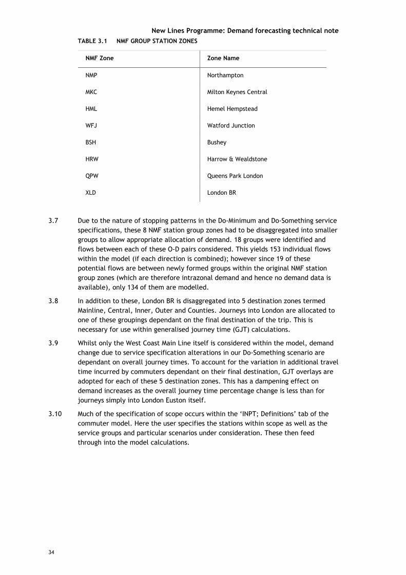
3.6 For the West Coast Main Line, 8 NMF group station zones are considered within the model; these are listed in Table 3.1.
New Lines Programme: Demand forecasting technical note
34
TABLE 3.1 NMF GROUP STATION ZONES
NMF Zone Zone Name
NMP Northampton
MKC Milton Keynes Central
HML Hemel Hempstead
WFJ Watford Junction
BSH Bushey
HRW Harrow & Wealdstone
QPW Queens Park London
XLD London BR
3.7 Due to the nature of stopping patterns in the Do-Minimum and Do-Something service specifications, these 8 NMF station group zones had to be disaggregated into smaller groups to allow appropriate allocation of demand. 18 groups were identified and flows between each of these O-D pairs considered. This yields 153 individual flows within the model (if each direction is combined); however since 19 of these potential flows are between newly formed groups within the original NMF station group zones (which are therefore intrazonal demand and hence no demand data is available), only 134 of them are modelled.
3.8 In addition to these, London BR is disaggregated into 5 destination zones termed Mainline, Central, Inner, Outer and Counties. Journeys into London are allocated to one of these groupings dependant on the final destination of the trip. This is necessary for use within generalised journey time (GJT) calculations.
3.9 Whilst only the West Coast Main Line itself is considered within the model, demand change due to service specification alterations in our Do-Something scenario are dependant on overall journey times. To account for the variation in additional travel time incurred by commuters dependant on their final destination, GJT overlays are adopted for each of these 5 destination zones. This has a dampening effect on demand increases as the overall journey time percentage change is less than for journeys simply into London Euston itself.
3.10 Much of the specification of scope occurs within the ‘INPT; Definitions’ tab of the commuter model. Here the user specifies the stations within scope as well as the service groups and particular scenarios under consideration. These then feed through into the model calculations.
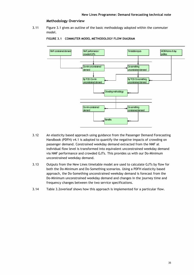
New Lines Programme: Demand forecasting technical note
35
Methodology Overview
3.11 Figure 3.1 gives an outline of the basic methodology adopted within the commuter model.
FIGURE 3.1 COMMUTER MODEL METHODOLOGY FLOW DIAGRAM
Do min constrained demand
Do something constrained demand
Crowding methodology
Benefits
Do min unconstrained demand
Do something unconstrained demand
By TOD: Do min unconstrained demand
By TOD: Do something unconstrained demand
NMF constrained demand NMF performance / crowded GJTs
Timetable inputs MOIRA time of day profiles
3.12 An elasticity based approach using guidance from the Passenger Demand Forecasting Handbook (PDFH) v4.1 is adopted to quantify the negative impacts of crowding on passenger demand. Constrained weekday demand extracted from the NMF at individual flow level is transformed into equivalent unconstrained weekday demand via NMF performance and crowded GJTs. This provides us with our Do-Minimum unconstrained weekday demand.
3.13 Outputs from the New Lines timetable model are used to calculate GJTs by flow for both the Do-Minimum and Do-Something scenarios. Using a PDFH elasticity based approach, the Do-Something unconstrained weekday demand is forecast from the Do-Minimum unconstrained weekday demand and changes in the journey time and frequency changes between the two service specifications.
3.14 Table 3.2overleaf shows how this approach is implemented for a particular flow.
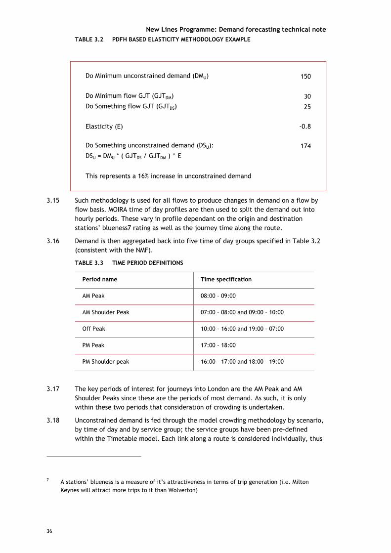
New Lines Programme: Demand forecasting technical note
36
TABLE 3.2 PDFH BASED ELASTICITY METHODOLOGY EXAMPLE
Do Minimum unconstrained demand (DMU) 150
Do Minimum flow GJT (GJTDM) 30Do Something flow GJT (GJTDS) 25
Elasticity (E) -0.8
Do Something unconstrained demand (DSU): 174DSU = DMU * ( GJTDS / GJTDM ) ^ E
This represents a 16% increase in unconstrained demand
3.15 Such methodology is used for all flows to produce changes in demand on a flow by flow basis. MOIRA time of day profiles are then used to split the demand out into hourly periods. These vary in profile dependant on the origin and destination stations’ blueness7 rating as well as the journey time along the route.
3.16 Demand is then aggregated back into five time of day groups specified in Table 3.2 (consistent with the NMF).
TABLE 3.3 TIME PERIOD DEFINITIONS
Period name Time specification
AM Peak 08:00 – 09:00
AM Shoulder Peak 07:00 – 08:00 and 09:00 – 10:00
Off Peak 10:00 – 16:00 and 19:00 – 07:00
PM Peak 17:00 - 18:00
PM Shoulder peak 16:00 – 17:00 and 18:00 – 19:00
3.17 The key periods of interest for journeys into London are the AM Peak and AM Shoulder Peaks since these are the periods of most demand. As such, it is only within these two periods that consideration of crowding is undertaken.
3.18 Unconstrained demand is fed through the model crowding methodology by scenario, by time of day and by service group; the service groups have been pre-defined within the Timetable model. Each link along a route is considered individually, thus
7 A stations’ blueness is a measure of it’s attractiveness in terms of trip generation (i.e. Milton
Keynes will attract more trips to it than Wolverton)

New Lines Programme: Demand forecasting technical note
37
allowing people to be crowded off as a train moves along the line. NMF crowding curves are used to obtain constrained load factors from the equivalent unconstrained load factors at each station, thus providing constrained demand by flow. The difference between these two figures provides us with the absolute number at any particular point along the line who have been crowded off.
3.19 The output from this methodology is both unconstrained and constrained demand for each scenario by flow, by time of day and by service group. This allows the calculation of individual journey time and crowding benefits for any particular flow.
Data Inputs
3.20 This section aims to provide further information on the datasets used within the model, along with any caveats to be aware of when interpreting their meaning.
Network Modelling Framework (NMF) Data
3.21 The NMF is a key source within the Commuter model for a number of different data inputs – demand data, revenue data, crowded and performance GJTs and crowding curves. The NMF run used is HLOS run 1584.
3.22 The NMF comprises 566 station group zones which represent geographical aggregations of all stations within the UK. Zones are referred to by the Primary station name with all demand from stations within the group being routed via this station.
3.23 Forecasts of constrained demand and revenue are output for each origin and destination pair of station group zones in 2030 (revenue is given in 2004/05 prices). In additional to this, crowded and performance GJTs are output for each flow. These represent the difference between the perceived generalised journey times of passengers in crowded or un-crowded conditions.
3.24 Crowding curves derived from NMF are also used within the model. These are pre-calculated curves which define the relationship between constrained and unconstrained load factors. The approach assumes that crowding costs can be defined in time equivalent terms and as such a crowding penalty can be viewed as a perceived % increase in journey time over a particular demand section. An elasticity approach based on PDFH can then forecast the decrease in demand due to crowded conditions. A process of iteration is then required, the equilibrium of which is our required constrained load factor.
3.25 These pre-calculated curves vary dependant on the level of commuters on a route, since values of time and therefore implied time penalties vary by journey purpose. Calculations of the journey purpose splits within our model are based upon data gleaned from the NRTS.
National Rail Travel Survey (NRTS)
3.26 The NRTS is a survey looking at passenger travel by rail throughout Great Britain. It is used within the model to provide information on journey purpose by ticket type.
3.27 It is used within the model to provide information on journey purpose by ticket type. Individual ticket types are assigned as being full, reduced or season tickets and the corresponding split of commuting to other journey purposes extracted. An estimate of the overall percentage of commuters on the line split by time of day which is used to choose the appropriate crowding curve is then calculated.

New Lines Programme: Demand forecasting technical note
38
3.28 The survey looks at Great Britain as a whole so is not disaggregated by specific route or region. To allow for this, data from the NMF is used to provide expected splits of tickets types across the whole commuter market under consideration, and the journey purpose splits adjusted appropriately.
New Lines Timetable Model
3.29 Service specifications have been produced for the Do-Minimum and Do-Something for both a standard peak and off-peak hour. These are inputs into the New Lines timetable model. Within this model, these are used to output journey times and frequencies for each flow as well as the proportion of passengers who would use each service group. This is achieved by assuming uniform demand throughout the peak hour period and the assignment of demand to trains according to the shortest journey time to their individual destinations.
3.30 Specification of these outputs is done so based on flows between primary stations in each newly defined NMF subgroup zone to ensure a consistent basis to the demand data. For the commuter model, journeys where an interchange between rail services is necessary are excluded from scope.
MOIRA Profiles
3.31 The model uses MOIRA time of day profiles to split demand out into hourly periods. These vary in profile dependant on the journey time along the route, flow type and on the origin and destinations’ ‘blueness’ rating. A stations’ blueness is a measure of it’s attractiveness in terms of trip generation.
Office of Rail Regulation (ORR) Station Usage Data
3.32 Data extracted from the NMF is on a station group zone basis and as such cannot provide demand data disaggregated by individual stations. When considering the variation in train stopping patterns however, it is necessary to have data at this level.
3.33 To achieve this, entries and exits from 2006/07 are taken from the ORR website in order to estimate the proportions using each station in 2030. This is then used to redistribute demand across newly defined subgroups before importing the data into the Commuter model. An implicit assumption here is that the distribution of demand across stations remains constant when comparing 2007 and 2030 entries and exits.
Detailed Review of Methodology
3.34 This section aims to expand on the methodology overview already provided. Broadly the commuter model methodology can be split into 5 main segments:
I Calculation of Do-Minimum unconstrained demand;
I Calculation of Do-Something unconstrained demand;
I Allocation by time of day and flow grouping;
I Crowding methodology; and
I Calculation of benefits.
New Lines Programme: Demand forecasting technical note
39
Calculation of Do-Minimum Unconstrained Demand
3.35 The Network Modelling Framework (NMF) has been used to generate Do-Minimum demand based upon 2030 forecasts. Constrained demand for full, reduced and season tickets from the NMF is extracted by flow; this is done so at both weekday and annual level. Data is fed through the model at a weekday level with the annual demand data being used latterly to calculate appropriate annualisation factors.
3.36 The scope of the Commuter model extends as far as Northampton in our West Coast Main Line test case and as such there are 8 NMF station group zones which are extracted. Stopping patterns in the Do-Minimum and Do-Something service specifications are not regular however across an entire NMF station group zone and therefore these 8 NMF station group zones have to be disaggregated into smaller groups to allow appropriate allocation of demand.
3.37 This is particularly relevant in our West Coast Main Line test case when considering the difference between DC Line trains and the rest of the line. The DC Line trains stop at all intermediate stations and are thus able to serve all passengers; conversely many of the other trains merely stop at the primary stations along the route. This clearly leads to a disparity in journey time and as a consequence, a tendency towards using the faster trains when considering service group allocation within the New Lines timetable model. In reality however, a proportion of this demand would have no option but to use the slower DC Lines.
3.38 Given that, the NMF station group zones were disaggregated as discussed previously. As demand data is not available for these NMF intrazonal flows, changes between such flows are not modelled. By the nature of the subgroup allocation process, such flows will be small and as such assuming no change between the Do-Minimum and Do-Something scenarios will have no major impact on the final outputs.
3.39 Crowded and performance GJTs for each flow are also extracted to enable the derivation of equivalent unconstrained demand from the NMF data. A standard elasticity based approach from PDFH v4.1 is adopted to undertake this conversion.
Calculation of Do-Something Unconstrained Demand
3.40 Having calculated the Do-Minimum unconstrained demand for each flow, the same PDFH based approach to forecast the Do-Something unconstrained demand is used. This relies on information with regards journey time and frequency extracted from the New Lines timetable model and based upon Do-Minimum and Do-Something service specification data. As such, the Do-Something unconstrained demand is the Do-Minimum unconstrained demand uplifted by the effect of service specification changes between the Do-Minimum and Do-Something service specifications.
3.41 For each in scope flow, frequencies, average journey times and distributions of demand in a peak hour period are extracted for both the Do-Minimum and Do-Something service specifications. It should be noted that within the commuter model, flows whereby an interchange is required are not considered within scope. For the vast majority of demand along the line however this is not an issue; indeed only 0.4% of demand in the Do-Minimum scenario is unaccounted for due to this omission.
3.42 In order to capture the intrinsic disparity in overall journey time experienced by travellers to London dependant on their actual final destination, overlays of
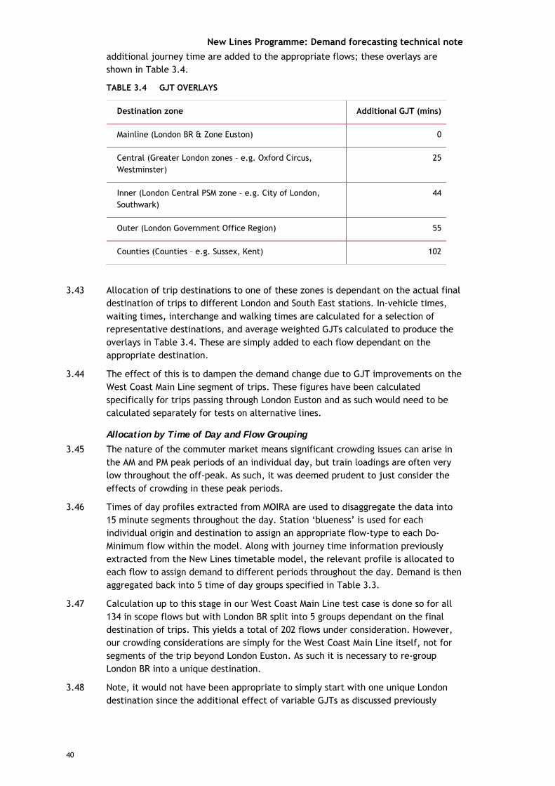
New Lines Programme: Demand forecasting technical note
40
additional journey time are added to the appropriate flows; these overlays are shown in Table 3.4.
TABLE 3.4 GJT OVERLAYS
Destination zone Additional GJT (mins)
Mainline (London BR & Zone Euston) 0
Central (Greater London zones – e.g. Oxford Circus, Westminster)
25
Inner (London Central PSM zone – e.g. City of London, Southwark)
44
Outer (London Government Office Region) 55
Counties (Counties – e.g. Sussex, Kent) 102
3.43 Allocation of trip destinations to one of these zones is dependant on the actual final destination of trips to different London and South East stations. In-vehicle times, waiting times, interchange and walking times are calculated for a selection of representative destinations, and average weighted GJTs calculated to produce the overlays in Table 3.4. These are simply added to each flow dependant on the appropriate destination.
3.44 The effect of this is to dampen the demand change due to GJT improvements on the West Coast Main Line segment of trips. These figures have been calculated specifically for trips passing through London Euston and as such would need to be calculated separately for tests on alternative lines.
Allocation by Time of Day and Flow Grouping
3.45 The nature of the commuter market means significant crowding issues can arise in the AM and PM peak periods of an individual day, but train loadings are often very low throughout the off-peak. As such, it was deemed prudent to just consider the effects of crowding in these peak periods.
3.46 Times of day profiles extracted from MOIRA are used to disaggregate the data into 15 minute segments throughout the day. Station ‘blueness’ is used for each individual origin and destination to assign an appropriate flow-type to each Do-Minimum flow within the model. Along with journey time information previously extracted from the New Lines timetable model, the relevant profile is allocated to each flow to assign demand to different periods throughout the day. Demand is then aggregated back into 5 time of day groups specified in Table 3.3.
3.47 Calculation up to this stage in our West Coast Main Line test case is done so for all 134 in scope flows but with London BR split into 5 groups dependant on the final destination of trips. This yields a total of 202 flows under consideration. However, our crowding considerations are simply for the West Coast Main Line itself, not for segments of the trip beyond London Euston. As such it is necessary to re-group London BR into a unique destination.
3.48 Note, it would not have been appropriate to simply start with one unique London destination since the additional effect of variable GJTs as discussed previously

New Lines Programme: Demand forecasting technical note
41
would be lost. The result of this would have been an over-estimate of the benefits of any service specification improvements. Having calculated each GJT change and thus demand change at a disaggregated level however, these can simply be summed to produce an overall change by our base 134 flows across the route.
3.49 It is also worth noting that at this stage the demand for each flow is halved in order to obtain the approximate one-way demand; only flows into London are considered and hence people are crowded off in the AM peak and Am shoulder peak only. This is then factored back up at the outputs stage to obtain the impact on two-way demand, assuming similar crowding impacts in the pm peak.
Crowding Methodology
3.50 The National Rail Travel Survey (NRTS) is used to provide information on the journey purpose by different ticket types. These are then allocated as full, reduced or season tickets to be comparable with our demand data. The survey looks at Great Britain as a whole so is not disaggregated by specific route or region. To allow for this, data from the NMF is used to provide expected splits of tickets types across the whole commuter market under consideration, and the journey purpose splits adjusted appropriately.
3.51 The balance of demand across ticket types is then used to calculate the percentage of commuters on the route in each time of day period. The average percentage of commuters across the AM peak and AM shoulder peak in our West Coast Main Line test case is 69%.
3.52 This is then used to extract the appropriate NMF crowding curve to be used within the crowding methodology.
3.53 When considering crowding along the line, data is fed through by scenario, service group and time of day. As discussed above, demand is allocated to each service group within the New Lines timetable model. After the aforementioned appropriate reallocation of some demand, this is then used to provide demand for any individual service group on a flow by flow basis.
3.54 The key feature of the methodology is that crowding is considered by individual link. As such, numbers on a particular service group and the implied load factors at any point along the line can be calculated. It is therefore possible to produce a profile of crowding whereby those further down the line are more susceptible to be crowded off.
3.55 Table 3.5 shows an example of the crowding methodology for a particular link.

New Lines Programme: Demand forecasting technical note
42
TABLE 3.5 CROWDING EXAMPLE – WATFORD JUNCTION TO BUSHEY LINK
Unconstrained arrivals at head station 1,750
De-constrained passengers carried forward 750
Total unconstrained demand on link 2,500
Total service group seating capacity 3,234
Total available seating capacity 2,734
Implied unconstrained load factor 91%
Equivalent constrained load factor 82%
Total constrained demand on link 2250
Total to be crowded off 250
3.56 Having established the demand for a particular scenario, service group and time of day, this provides us with arrivals at the head station of a particular link. Table 6.3 shows that there are 1,750 unconstrained arrivals at Watford Junction.
3.57 This is then added to the demand carried forward from the previous link, less those getting off at the head station. Demand carried forward at the start of the route, in our test case Northampton, is assumed to be zero (in most cases, see further discussion below) else it is the calculated demand from all previous links. Note that the carried forward demand is output in constrained terms, and as such must be de-constrained using NMF crowding curves first in order to be input on a consistent basis as the arrivals. In the example above, this gives us 750 de-constrained passengers carried forward from further up the line (i.e. having boarded at stations between Northampton and Hemel Hempstead).
3.58 The total unconstrained demand offered on the link is simply the sum of these two; 2,500 people in this example. The next stage is to consider the total capacity of any particular service group. The particular rolling stock considered here are 11-car class 390 which have 577 seats.
3.59 The NMF crowding curves work off proxy seats for any particular rolling stock, which in this case is 539 seats. This adjustment is to account for the variation across rolling stock in balance of seating and standing capacity. Where high-density rolling stock is used, more capacity is set aside for standing as opposed to seating, and as such simply using the seating capacity in our calculations would over-estimate crowding issues. Proxy seats are used to uplift this effective seating capacity to take account of this balance.
3.60 The particular example being considered above would have 6 trains per hour in the AM peak period, thus yielding a total capacity of 3,234.
3.61 Whilst most service groups are effectively self-contained services from Northampton or closer to London Euston, some would be used by passengers from further up the line. The scope of this model does not incorporate such demand as it starts outside our designated commuter zone; dependant on the exact flow, it would be

New Lines Programme: Demand forecasting technical note
43
considered within one of the other two New Lines demand models. To avoid any possibility of double-counting, these people are excluded from the commuter model. However, their effects in terms of train crowding does need to be taken account of.
3.62 To deal with this, outputs from the New Lines regional model are extracted for all flows into London for both the Do-Minimum and Do-Something scenarios and input into the commuter model. In a similar process to the Do-Minimum and Do-Something commuter service specifications, demand from these stations are allocated to a particular service group. These flows are then treated in the same way as our commuter demand (i.e disaggregated by time of day and direction) to give us the total demand from all of these stations by scenario, by service group and by time of day. Since these people are arriving first onto the trains, they are then allocated seats all the way into London by reducing the effective seating capacity on each train. In this way, their effect in terms of crowding is felt but they are not included in any demand calculations undertaken. In the example in table 6.3, this pre-loaded is taken to be 500 and thus reduced the effective capacity by this amount down to 2,734.
3.63 The unconstrained load factor is then simply calculated by dividing the total unconstrained demand by the effective capacity. This gives us an implied load of 91%. Looking up the appropriate values on our NMF crowding curve, this gives an equivalent constrained load factor of 82%.
3.64 Applying this constrained load factor to our calculated effective capacity provides us with the total constrained load for our link; in this case 2,250. The number to be crowded off is then the difference between the total unconstrained and constrained demand; in our example this means 250 people must be crowded off this link.
3.65 Having determined the absolute number to be crowded off the link, the model then determines who should be crowded off and from where. The first people to be crowded off are those who are forced to stand as they are more adversely affected by crowded conditions than those who are able to sit. If there are seats available, everyone on the train is assumed to occupy them and therefore there are no people standing until the unconstrained load factor exceeds 100%. The nature of the link based process means that those already on the train are allocated seats first and as such, new boarders are more likely to have to stand and consequentially more likely to be crowded off.
3.66 In our example however, the unconstrained load factor is less than 100% so everyone is able to sit. Therefore the 250 people to be crowded off must be from seated passengers. Note that crowding is assumed to result in a decrease in demand prior to 100% load. This is the approach taken in the NMF as perceived journey times increase after the load factor rises above 60%.
3.67 Once allocation of new arrivals and carried forward demand to be either standing or sitting has been undertaken, they are treated as being equally likely to be crowded off. The logic behind this is that all will be experiencing the same conditions and thus have the same propensity to chose not to travel by rail in crowded circumstances. Allocation of those to be crowded off is therefore done proportionally to the absolute number of boarders and carried forward demand. In our example, this means that 70% (175 passengers) and 30% (75 passengers) of those crowded off are boarders and carried forward passengers respectively.
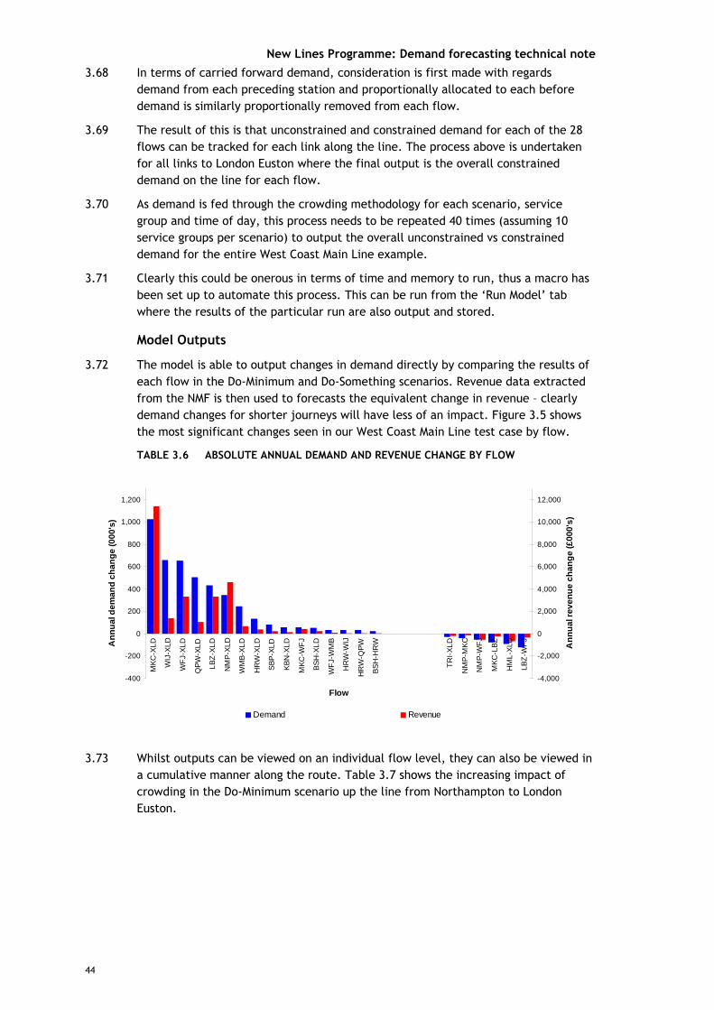
New Lines Programme: Demand forecasting technical note
44
3.68 In terms of carried forward demand, consideration is first made with regards demand from each preceding station and proportionally allocated to each before demand is similarly proportionally removed from each flow.
3.69 The result of this is that unconstrained and constrained demand for each of the 28 flows can be tracked for each link along the line. The process above is undertaken for all links to London Euston where the final output is the overall constrained demand on the line for each flow.
3.70 As demand is fed through the crowding methodology for each scenario, service group and time of day, this process needs to be repeated 40 times (assuming 10 service groups per scenario) to output the overall unconstrained vs constrained demand for the entire West Coast Main Line example.
3.71 Clearly this could be onerous in terms of time and memory to run, thus a macro has been set up to automate this process. This can be run from the ‘Run Model’ tab where the results of the particular run are also output and stored.
Model Outputs
3.72 The model is able to output changes in demand directly by comparing the results of each flow in the Do-Minimum and Do-Something scenarios. Revenue data extracted from the NMF is then used to forecasts the equivalent change in revenue – clearly demand changes for shorter journeys will have less of an impact. Figure 3.5 shows the most significant changes seen in our West Coast Main Line test case by flow.
TABLE 3.6 ABSOLUTE ANNUAL DEMAND AND REVENUE CHANGE BY FLOW
-400
-200
0
200
400
600
800
1,000
1,200
MKC
-XLD
WIJ
-XLD
WFJ
-XLD
QPW
-XLD
LBZ-
XLD
NM
P-XL
D
WM
B-XL
D
HR
W-X
LD
SBP-
XLD
KBN
-XLD
MKC
-WFJ
BSH
-XLD
WFJ
-WM
B
HR
W-W
IJ
HR
W-Q
PW
BSH
-HR
W
TRI-X
LD
NM
P-M
KC
NM
P-W
FJ
MKC
-LBZ
HM
L-XL
D
LBZ-
WFJ
Flow
Ann
ual d
eman
d ch
ange
(000
's)
-4,000
-2,000
0
2,000
4,000
6,000
8,000
10,000
12,000
Ann
ual r
even
ue c
hang
e (£
000'
s)
Demand Revenue
3.73 Whilst outputs can be viewed on an individual flow level, they can also be viewed in a cumulative manner along the route. Table 3.7 shows the increasing impact of crowding in the Do-Minimum scenario up the line from Northampton to London Euston.

New Lines Programme: Demand forecasting technical note
45
TABLE 3.7 DO-MINIMUM CONSTRAINED VS UNCONSTRAINED DEMAND
0
5,000
10,000
15,000
20,000
25,000
NM
P-M
KC
MKC
-LBZ
LBZ-
TRI
TRI-H
ML
HM
L-W
FJ
WFJ
-WFH
WFH
-BSH
BSH
-CPK
CPK
-HTE
HTE
-HR
W
HR
W-K
NT
KNT-
WM
B
WM
B-SB
P
SBP-
WIJ
WIJ
-QPW
QPW
-KBN
KBN
-XLD
Flow
Ann
ual d
eman
d (0
00's
)
Unconstrained demand Constrained demand
3.74 As you would expect given the crowding methodology, the number crowded off increases as you move close to London Euston, hence the increased disparity between the unconstrained and constrained demand.
3.75 Outputs comparing such results between the two scenarios are able to help inform the users of where the introduced Do-Something service specification is working well in comparison to the Do-Minimum.
3.76 A fundamental part of the model outputs is to produce information to be exported into the New Lines appraisal model. There are 6 key outputs for this:
I Do-Minimum demand
I Do-Something demand
I Revenue generation
I Change in passenger miles
I Journey time benefits
I Crowding benefits.
3.77 Demand outputs are extracted directly from the crowding methodology and annualised using annualisation factors out of the NMF. Average revenue per trip is extracted again from the NMF to convert this demand into anticipated annual revenue. Changes in passenger demand are converted into changes in passenger miles simply by applying distance factors to each individual flow.
3.78 Outputs from the crowding methodology give us unconstrained and constrained demand in the AM peak and AM shoulder peak by flow. Since crowding is not considered an issue in the off peak, these two demand figures are the same for the off peak period and can simply be extracted from our calculated demand by time of day. In order to calculate journey time and crowding benefits for each flow,

New Lines Programme: Demand forecasting technical note
46
demand is aggregated into peak and off-peak periods to allow the appropriate use of peak or off-peak un-crowded GJTs.
3.79 It should be noted that all appraisal outputs are subsequently doubled to account for the fact that the model only looks at one-way demand. Underlying this is the assumption that all trips made into London by rail invariably need to be made again from London. This seems reasonable since the choice of mode of travel is made in the inbound trip, not the outbound in most cases; this is particularly applicable to the commuter market.
3.80 There is also an implicit assumption that the pm peak period is the reversal of the am peak period. It should be noted that the am peak is, in general, more peaked than the pm peak period so this assumption will lead to a slightly higher forecast of crowding in the pm peak than may occur in reality. However this overestimate will be of a small magnitude.
3.81 Crowded GJTs are then calculated using a standard elasticity based approach from PDFH v4.1. This in conjunction with un-crowded GJTs, unconstrained and constrained demand is used to calculate journey time and crowding benefits for each flow.
3.82 Existing users experience a journey time benefit equal to the absolute change in Do-Minimum to Do-Something un-crowded GJT. Newly generated users are assumed to experience only half this benefit.
3.83 Crowding benefits are calculated dependant on the ratio of change between the two scenarios’ crowded and un-crowded GJTs. This ensures that any absolute journey time benefit is removed before crowding is considered, thus avoiding the possibility of double-counting benefits. The model outputs both of the benefits by individual weekday trip, and as such they must be annualised using the same factors as the demand to obtain total annual benefits for any particular flow.

New Lines Programme: Demand forecasting technical note
47
4 Regional Model
Introduction
4.1 This Chapter focuses on the model for regional services on the classic network, a market segment often characterised by less frequent trains, higher in-vehicle times and less direct services. The construction of New Lines could alleviate these issues, and thereby increase demand for these services, by facilitating a recast of the timetable on the entire classic network.
4.2 The Regional Model measures the impacts on demand of changes in frequencies, in-vehicle times and interchanges, but not from changes in levels of crowding; this is deemed only to be a material issue on intercity and commuter services.
4.3 There are three main types of data used in the regional model: demand data provided by the NMF (Network Modelling Framework), service specification data and parameters provided by PDFH. The model uses the parameters from PDFH to estimate the effect of the service specification data on the demand data from the NMF.
4.4 It should be noted that as with the commuter model the regional model does not model changes in fares; this means that fares are implicitly assumed to remain unchanged between the DM and DS scenarios. Also note that the model applies PDFH methodologies, which are known to underestimate the impacts on demand of large changes in generalised journey times.
Scope of the Model
4.5 The Regional model has been populated solely with West Coast Main Line demand and service specification data. There are 41 stations designated as ‘in-scope’ for this route; these 41 stations represent those stations on the West Coast Main Line which are designated as NMF ‘primary stations’.
4.6 As well as flows between these 41 stations, the Regional model also includes flows that lie partially on the West Coast Main Line but that begin and / or end at stations on a different line. These flows are handled by defining of six external zones and by assigning each of these zones with an ‘add-on’ generalised journey time, which is added to the GJT calculated for the portion of the journey lying on the WCML.
4.7 For the West Coast Main Line, Northampton was identified as the limit of scope for the Commuter Model. Whilst there will clearly be a limited number who commute into London Euston from beyond Northampton, the majority of commuting journeys are from within this boundary so flows from further afield were deemed out of scope for the Commuter Model.
4.8 It should be made clear that all the demand models were designed and built to be able to model any route. The models have all been designed in a generic way that should, in theory, enable them to be easily transferable to other lines simply by inputting the appropriate demand and service specification data.
New Lines Programme: Demand forecasting technical note
48
Methodology Overview
4.9 As previously outlined, the Regional Model forecasts changes in demand resulting from changes in frequency, in-vehicle times and interchanges, for services on the classic network. The service specification data used is for a standard hour and the model assumes that the service specification at each station is identical in both directions and remains the same throughout the day.
4.10 The model calculates Do-Minimum and Do-Something generalised journey times from the service specifications and then uses an elasticity-based approach to forecast changes in demand (and revenue) as a function of the proportional changes in generalised journey time.
Data Inputs
Network Modelling Framework (NMF)
4.11 The NMF comprises 566 zones which together represent all stations in the UK; zones are referred to by their primary station name, and for modelling purposes it is assumed that all demand from stations within the zone is routed via this station. Demand and revenue forecasts for 2030 are output for each zone pair (revenue is given in 2004/05 prices).
4.12 The NMF also provides the x and y coordinates of all primary stations, which were used to estimate the distances between stations by first calculating the straight-line distance then adding a 20% uplift. This information was used for the calculation of interchange penalties and the change in passenger miles between the Do Minimum and Do Something options (the latter is then output to the Appraisal Model).
4.13 It should be noted that due to the relatively coarse zoning of the demand data the regional model should not be used to optimise a service specification. It is designed to estimate the likely value of a defined service specification.
New Lines Timetable Model
4.14 Do-Minimum and Do-Something service specifications are fed as inputs into the Timetable Model. The Timetable Model processes these inputs and outputs frequencies, in-vehicle times and the number of interchanges required, for each primary station to primary station flow.
4.15 These outputs are based on flows between primary stations to ensure consistency with the demand and revenue data from the NMF. Journeys requiring two or more interchanges were excluded entirely from the timetable model, and therefore also from the regional model, because the number of possible journeys becomes to large to work with when more than one interchange is considered.
Detailed Review of Methodology
4.16 There are three key methodological components of the regional model: the first involves designating the flows that are ‘in-scope’ for the model, the second involves obtaining a generalised journey time for each of these flows, and the third involves using these generalised journey times to forecast changes in demand and revenue. These three components are all described in detail in this section. The second component is the more difficult of the three to implement as converting service specification data into generalised journey times is a complex task.

New Lines Programme: Demand forecasting technical note
49
Designation of In-scope Flows
4.17 The flows that should be modelled in the regional model vary depending on the option being tested. Any flows that would use the New Line are modelled in the Inter city model rather than the regional model. For example in the case of an option that just featured New Line services between London, Birmingham and Manchester flows between London and Liverpool would fall within the scope of the regional model. However if the New Line services also served the London to Liverpool market this flow would then be modelled in the Inter city model and would have to be excluded from the regional model to avoid double counting. Therefore for each model run a number of flows are designated as being out of scope for the regional model.
4.18 For each option tested in the model a set of station groups is defined, with each group corresponding to one of several predefined locations (note that although the groupings vary across the different options, the list of locations remains constant). An example of one of the station groupings used can be seen in Figure 4.1.
FIGURE 4.1 EXAMPLE OF STATION GROUPINGS
Group Stations
LancasterCumbriaEdinburghTrent Valley
WarringtonLiverpoolPrestonGlasgow
LondonBirminghamManchester
BusheyHarrow and WealdstoneWembley CentralWolverhamptonCheadle Hulme
RuncornChester
Motherwell
Oxenholme Lake District
Queens ParkSandwell and Dudley
Stockport
Liverpool Lime StreetWigan North Western
Blackpool North
StaffordEdinburghTamworth. Lichfield Trent Valley
Glasgow CentralLancaster
Carlisle
London EustonBirmingham New Street
Manchester Piccadilly
Liverpool Sth Pway AllertoWarrington Bank Quay
Preston
4.19 Flows between all stations in one group and all stations in another group are then designated as either in-scope or out-of-scope, depending on the particular configuration of the option being tested. Specifically, if two locations in the list are directly connected on the New Line then flows between the corresponding groups are deemed out-of-scope.
4.20 Each location therefore represents a proposed New Lines station (with the exception of Trent Valley), and the groupings represent the catchment areas of these proposed stations. The reason for allowing these groupings to vary across the different options is that the catchment area of a particular New Lines station will depend on the option being tested.
4.21 In practice, the groupings used for each option tested are almost identical to those given in above. The only differences between the options are in the Warrington and Preston groups; by default, Wigan North Western was taken to be in the Warrington group, but if there was no New Lines station at Warrington and one at Preston then it was moved to the Preston group.
4.22 The Trent Valley group was included in the list so as to be able to designate flows between Trent Valley stations and Birmingham stations as out-of-scope. Although these journeys can be done purely or partially on the West Coast Main Line, in practice they would not be and therefore are excluded from the Regional Model.
4.23 Note that, with the exception of the Trent Valley to Birmingham flows, when designating which group pairs were in-scope for the Regional Model care was always taken to designate the corresponding flows as out-of-scope for the Intercity Model. This ensured that there was no omission or double counting of results.

New Lines Programme: Demand forecasting technical note
50
GJT Calculations
4.24 The first step in setting up the GJT calculations involved defining a methodology for specifying which services between a given pair of stations would be designated as ‘attractive’. The rationale was that only relatively fast services will be considered attractive by passengers; slower services are effectively ignored and should therefore be excluded from the GJT calculations.
4.25 For each flow a ‘cut-off’ in-vehicle time was defined and only services with in-vehicle times less than or equal to this cut-off were deemed to be attractive. This cut-off in-vehicle time was obtained by multiplying the minimum in-vehicle time for the flow with a frequency-dependent ‘fast-slow multiplier’, and, if the minimum in-vehicle time was less than 30 minutes, adding an extra five minutes. The additional of five minutes was designed to avoid anomalies such as a 12 minutes journey being deemed as slow where the faster services was only two minutes quicker.
4.26 Of the numerous approaches tested, this was found to give the most intuitively plausible division of services into attractive and non-attractive categories. Table 4.1 shows the lookup table used to calculate the fast-slow multipliers.
TABLE 4.1 LOOKUP TABLE USED TO CALCULATE FAST-SLOW MULTIPLIERS
Frequency (trains per hour) Multiplier
2 1.5
3 1.35
4+ 1.25
4.27 The next step in setting up the GJT calculations involved defining the add-on generalised journey times for flows not lying entirely on the West Coast Main Line, by considering typical ‘cross-London’ journeys to from London Euston to each of the London external zones and calculating the corresponding GJTs. The numbers used in the model are shown in Table 4.2.
TABLE 4.2 LOOKUP TABLE USED TO CALCULATE ADD-ON GENERALISED JOURNEY TIMES
Area Add-on GJT (mins)
Mainline terminus 0
Central London 25
Inner London 44
Outer London 55
Home counties 102
Remote 150

New Lines Programme: Demand forecasting technical note
51
4.28 The GJT for a given flow, and for a given ticket type, was calculated using the following standard PDFH formula:
GJT = wait time + journey time + interchange penalty + add-on GJT.
4.29 The wait times were obtained from the PDFH lookup table (shown in Table 4.3).
TABLE 4.3 WAIT TIME PENALTIES BY TICKET TYPE (MINS)
Service interval Full Reduced Season
5 5 5 5
10 10 10 10
15 15 14 15
20 19 17 19
30 26 21 26
40 31 23 31
60 39 27 39
90 51 33 51
120 63 39 63
180 87 51 87
4.30 The PDFH lookup table used to calculate the interchange penalties is shown in Table 4.4. The actual interchange penalty for a given flow was obtained using a straight-line interpolation between the nearest two distances explicitly given in this lookup table, except if the flow’s distance was greater than 325 miles, in which case the penalties for a flow with a distance of 325 miles were used.

New Lines Programme: Demand forecasting technical note
52
TABLE 4.4 INTERCHANGE PENALTIES BY TICKET TYPE (MINS)
Journey distance Full Reduced Season
0 10 10 7
15 15 15 10
30 19 19 12
50 25 25 16
70 31 31 20
100 40 40 26
150 55 55 36
200 65 65 36
300 85 85 36
325 90 90 36
4.31 Two GJTs were calculated for each flow / ticket type combination, one including only attractive direct services and the other including attractive direct services and interchange services. The actual GJT was then taken as the smaller of the two, the rationale being that if the GJT obtained using the interchange services is larger then the interchange services will effectively be ignored by passengers.
Forecasting Changes in Demand and Revenue
4.32 The Do-Minimum demand in the Regional Model was based on 2030 constrained demand forecasts for full, reduced and season tickets, obtained from the NMF. The model works at the annual level, but weekday demand is also fed through the model in order to provide ‘pre-loading’ outputs for the Commuter Model.
4.33 There are 41 stations designated as in-scope for the West Coast Main Line, of which 8 lie in the commuter corridor, giving a total of 41*41–8*8 = 1,617 in-scope flows lying entirely on the WCML. However, due to the inclusion of flows beginning and / or ending on a different line, the actual number of flows in the model is much larger than this at 4,016.
4.34 Having calculated the Do Minimum and Do Something GJTs as described above, the model uses the PDFH elasticity-based approach to forecast Do Something demand. An elasticity of -0.9 was used for Full, Reduced and Season ticket types, in accordance with PDFH recommendations.
4.35 Since fares are assumed to remain constant in the Regional Model, changes in revenue are calculated in exactly the same way as changes in demand are calculated. Fares are taken from the NMF, expressed as 2030 values to a 2004/5 price base. An uplift factor of 9.8% is applied to convert the revenue into 2007 prices, for consistency with the overall modelling framework.

New Lines Programme: Demand forecasting technical note
53
4.36 Given that the Do Something timetable has not been optimised for interchanges in the same way the Do Minimum timetable has, only flows with an absolute GJT change of greater than 10% were included in the calculations to avoid spurious results.
Model Outputs
4.37 The Regional Model aims to assess the impacts of New Lines on demand and revenue for regional services on the existing network, and the model therefore outputs key indicators of these impacts. An example of the outputs produced by the model is given in Figure 4.2 (these figures are for revenue – similar outputs can be produced for demand).
FIGURE 4.2 EXAMPLE OF OUTPUTS PRODUCED BY THE REGIONAL MODEL
Total Revenue Total Revenue IncreaseDM DS Proportional Absolutem /yr m /yr m /yr
£460.8 £488.5 6.0% £27.7
Top Flows by Absolute ChangeIncrease Orig Name Dest Name/yr
£4,129,311 London Euston Nuneaton£3,502,133 London Euston Rugby£3,152,669 London Euston Lichfield Trent Valley£2,533,330 London Euston Telford Central£2,398,032 London Euston Shrewsbury
Bottom Flows by Absolute ChangeIncrease Orig Name Dest Name/yr
-£1,003,239 London Euston Stoke-on-trent-£360,995 Wilmslow Manchester Piccadilly-£221,589 Warrington Bank Quay Glasgow Central-£159,077 Macclesfield Manchester Piccadilly-£149,351 London Euston Hartford
4.38 In addition, the model provides flow-level graphical diagnostics to help ensure that the results produced are sensible. An example of one of these diagnostics is given in Figure 4.3, which shows the distribution of demand increases for all flows where the demand increases by more than 10,000 passengers per year (this 10,000 is an input that can be easily changed to produce a different graph).

New Lines Programme: Demand forecasting technical note
54
FIGURE 4.3 DISTRIBUTION OF DEMAND INCREASES GREATER THAN 10,000 PAX PER YEAR
Distribution of Demand Increases
-150,000
-100,000
-50,000
0
50,000
100,000
150,000
200,000
0 5 10 15 20 25 30 35 40
Dem
and
Incr
ease
(pax
/yr)
4.39 The model also provides station-level graphical diagnostics to help ensure that the results produced are consistent with the timetable inputs. An example of one of these diagnostics is given in Figure 7.3, which shows the total absolute changes in demand and revenue for all flows beginning or ending at each of the 41 NMF primary stations on the West Coast Main Line.
FIGURE 4.4 DISTRIBUTION OF DEMAND AND REVENUE INCREASES BY STATION
Absolute Increases by NMF Station Group
-0.2
0.0
0.2
0.4
0.6
0.8
1.0
Lond
on E
usto
nQ
ueen
s Pa
rkH
arro
w &
WBu
shey
Wat
ford
JH
emel
HM
ilton
K C
Nor
tham
pton
Rug
byC
oven
tryBi
rmin
gham
IBi
rmin
gham
NSa
ndw
ell &
DW
olve
rham
pton
Telfo
rd C
Shr
ewsb
ury
Nun
eato
nTa
mw
orth
.Li
chfie
ld T
VSt
affo
rdSt
oke-
on-tr
ent
Cre
we
Mac
cles
field
Wilm
slow
Che
adle
Hul
me
Sto
ckpo
rtM
anch
este
r PC
hest
erH
artfo
rdR
unco
rnLi
verp
ool L
SW
arrin
gton
B Q
Wig
an N
WP
rest
onBl
ackp
ool N
Lanc
aste
rO
xenh
olm
e L
DC
arlis
leM
othe
rwel
lG
lasg
ow C
Edin
burg
h
Abs
olut
e In
crea
se (m
pax
/yr)
-£5
£0
£5
£10
£15
£20
£25
Abs
olut
e In
crea
se (m
/ yr
)
Demand Revenue

New Lines Programme: Demand forecasting technical note
55
4.40 The Regional Model produces the following outputs, by ticket type, to be fed into the New Lines Appraisal Model:
I Do Minimum demand;
I Do Something demand;
I revenue generation;
I change in passenger miles;
I journey time benefits; and
I crowding benefits.
4.41 Finally, weekday demand is also fed through the model in order to provide ‘pre-loading’ outputs for the Commuter Model. This demand is treated in exactly the same way as the annual demand in the model itself, but it is only output for flows between London Euston and those stations lying outside the commuter corridor.

New Lines Programme: Demand forecasting technical note
57
5 Heathrow Access Model
Introduction
5.1 Construction of a New Line to serve the West Midlands, the North West and Scotland for journeys into London could potentially encourage mode shift away from road and air for journeys accessing Heathrow for onward air travel. This effect could be increased by serving Heathrow directly, either routing a New Lines via Heathrow or via a diverging main line. This chapter details the analysis undertaken and model developed to assess the potential scale of such modal shift.
5.2 Under consideration is interlining and surface access demand into Heathrow; wholly domestic demand is considered in the Intercity model and as such is not included here.
5.3 The Heathrow Access Model has not been modelled to the same level of detail and rigour of the domestic New Lines models. As such, all results should be treated as “indicative estimates” only.
Model Development and Calibration
Model Structure
5.4 The Heathrow Access Model is a simple multinomial mode choice model looking across all the access (main) modes to Heathrow, namely air (interlining), rail, car and coach. There is no segmentation, all demand being treated as a single market.
Data Inputs and Scenarios
5.5 Calibration of the mode split model was undertaken using 2007 data before forecasting demand to 2030 (see discussion in ‘Model Forecasting’ section). Data was obtained from the CAA Airport flow report with regards air demand into Heathrow. This provides numbers of business and leisure interlining passengers in 2007 from all UK airports. Given the scope of the proposed New Line, only demand from Edinburgh, Glasgow and Manchester airports has been considered.
5.6 Surface access demand levels were obtained via the CAA Passenger Survey Report 2007/2008. This is used to provide 2007 levels of demand from car, coach (inc. all forms of road based public transport) and rail. The two datasets together provide an overall picture of current demand levels into Heathrow.
5.7 Additional data was purchased from the CAA to allow further disaggregation of this data at country and district level. In accordance with the aforementioned scope, the model considers demand for districts within the West Midlands, North West and Scotland who are deemed to potentially benefit from a new high speed line.
5.8 We have estimated 2007 Generalised Journey Time (GJT) costs at county level for air, coach, car and rail using existing (publicly available) datasets and information available on the internet. Consideration was given to real and perceived costs incurred due to headway, journey time, fare, interchange penalties and access times at both ends of the journey. Weightings, as employed in the Intercity model, were assigned to each of these components based on research into the relative importance of each cost for each mode.

New Lines Programme: Demand forecasting technical note
58
Calibration
5.9 The core model is applied as a multi-modal incremental logit model; this is consistent with WebTAG guidance and better represents the changes in modal shares afforded by New Lines where some modes currently have a low share, but where the journey cost is arguably prohibitive. This was particularly important with regards Scottish demand allocation to modes other than air. Although such demand is low, there is a current market which an absolute choice model would effectively ignore.
5.10 Estimation of the model parameters is undertaken via optimisation of a model error parameter based on the percentage errors of each individual forecast. Based on current input parameters, the model calculates the anticipated demand for each mode by county and compares this to known current demand from the aforementioned data sources to produce a percentage error. Each error is then weighted according to user inputs and summed to obtain an overall model error.
5.11 Next the model incrementally changes each parameter that the user defines as variable to try to find a more optimal solution. For each change, the model error is calculated in order to ascertain the best option. When a solution which further reduces the model error is found, the current parameters are replaced with these new ones and the process is repeated.
5.12 This process is automated within the model via a macro. The macro is stopped after a maximum of 400 runs, though in practice a solution is often found significantly before this point is reached.
5.13 A multitude of solutions can be obtained dependant on variations of weighting for each element of the model error or the limits of acceptable values that parameters are allowed to take. After significant testing of the model approach, it was decided most appropriate to assume a simple uniform weighting across all model error elements. In this way, the square difference between the modelled and observed demand is the only attribute of the model error.
5.14 Mode constants were fixed at 0 for both coach and car and at -40 for air travel. Testing of the model has shown these simple parameters to be effective with regards calibration and forecasting. It also avoids any possibility of calibration producing constants outside reasonable bounds.
Model Forecasting
5.15 Consistent with the forecasting framework, a forecast year of 2030 has been assumed. DfT forecasts suggest demand from Heathrow will increase by 100% from 2005 levels by 2030. A high level assumption that our overall market in 2030 would therefore be twice that of our 2007 demand has been made.
5.16 Assumptions with regards the future 2030 costs of travel for each mode were made in order to forecast our 2030 Do Minimum mode shares. For the classic rail network, the assumptions are consistent with the service specification set out in our Do Minimum scenario used in both the Commuter and Regional models.
5.17 Assumptions with regards fare growth and journey time changes (e.g. due to increased road congestion) are also made where applicable. This provides us with the perceived cost of journeys by each mode into London Heathrow, and as such a basis for forecasting our Do Minimum shares.

New Lines Programme: Demand forecasting technical note
59
5.18 Calculation of the individual market share of each mode for each county takes the form of an incremental logit model as shown below:
( )[ ]( )[ ]{ }∑
=
−××
−××= n
jBFB
BFBF
jjj
iii
i
CCsP
CCsPP
1exp
exp
Future year % market share for mode i
Base year % market share for mode i
Base year % market share for modes j = 1 to n
Future year perceived cost (inc. mode constant) for mode i
Base year perceived cost (inc. mode constant) for mode i
Future year perceived cost (inc. mode constant) for modes j = 1 to n
Base year perceived cost (inc. mode constant) for modes j = 1 to n
General scaling parameter
Number of modes under consideration
5.19 This yields the forecast proportion of demand in our Do Minimum scenario for each mode in each district under consideration.
5.20 To forecast the potential effect of a New Line, equivalent costs are then calculated for any given option. It is assumed within the model that classic rail passengers would switch to New Lines whenever this yields a lower GJT. As such, only a generic rail mode is considered within the model (though it should be noted that weightings attributed to New Lines as opposed to classic rail do differ when calculating GJTs, and in this way the perceived cost benefits due to modal preference between classic and new rail are reflected).
5.21 As with the forecasting of Do Minimum demand, Do Something costs are run through the model which outputs the anticipated proportion of demand for each mode. Applying this to the forecast market (discussed above), the expected numbers on each mode in each scenario is obtained, and as such the magnitude of extracted demand off air and road and onto rail. An example of this process is given below.
Example
5.22 Table 5.1 gives an example of the forecast Do Minimum demand shares for each mode in Scotland; Table 5.2 gives the forecast Do Minimum and Do Something GJT costs. The particular Do Something scenario under consideration envisions a half-hourly service from both Edinburgh and Glasgow (with those from Edinburgh having to interchange at Preston) with a journey time of just over 3 hours into Heathrow Airport.
==
=
=
=
=
=
=
=
ns
C
C
C
C
P
P
P
j
j
i
i
j
i
i
B
F
B
F
B
B
F

New Lines Programme: Demand forecasting technical note
60
TABLE 5.1 2007 BASE YEAR DO MINIMUM % OF DEMAND BY MODE FOR SCOTLAND
Car Air Coach Rail
2.1% 93.9% 1.6% 2.5%
TABLE 5.2 GJT COSTS (PERCEIVED MINS) BY MODE FOR SCOTLAND
Car Air Coach Rail
Base year 363 133 698 381
Future year 366 106 746 215
5.23 Application of the model yields a forecast mode share of rail from Scotland of 21.7%. The corresponding shares for car, air and coach would be 1.0%, 76.9% and 0.4% respectively. It should be noted that these figures are for all of Scotland. And as such air would remain the quickest mode for a significant number of O-D pairs.
Model Outputs
5.24 As well as forecasting absolute changes in annual demand as a result of a new high speed line, the Heathrow Access Model produces other outputs:
I Do-Minimum and Do-Something Demand;
I Change in annual revenue by mode;
I Change in road passenger km’s;
I Change in actual rail journey time;
I Change in perceived rail journey time; and
I Change in rail user charges.
5.25 These are standard outputs from the model whenever an option is tested and can be used within economic appraisals of new line options.
5.26 As discussed above, the Heathrow access model has not been modelled to the same level of detail and rigour of the domestic New Lines models. As such, all results should be treated as “indicative estimates” only.
New Lines Programme: Demand forecasting technical note
61
6 Near Europe Model
Introduction
6.1 The introduction of a New Line from the West Midlands, the North West and Scotland to London will reduce the overall rail journey time from principal cities in the United Kingdom to mainland Europe. This Chapter outlines the development and application of a simple mode choice model to estimate the amount of rail demand that could be abstracted from air four principal UK cities; Birmingham, Manchester, Glasgow and Edinburgh to two major European cities; Paris and Brussels (via HS1) as a result of New Lines interventions in the UK.
6.2 The air demand for each flow in 2030 has been estimated using CAA Airport flow data and DfT forecasts for short haul growth from UK airports from 2005 to 2030.
6.3 Two scenarios have been considered, both assuming a New London terminal at or near St.Pancras. The first involves an interchange between New Lines services and Eurostar trains at St. Pancras; the second scenario involves a direct service to Europe that calls at St. Pancras but without passengers changing trains.
6.4 For the model development, information about observed rail:air mode shares on Eurostar services in 2008 has been used to estimate the model parameters. The Generalised Journey Time (GJT) costs for air and rail have been calculated using existing datasets and information available on the internet.
6.5 As with the Heathrow Access model. The results from this model should be treated as “indicative estimates” only as they have not been modelled to the same detail and rigour as the domestic New Lines models.
Scope of the Model
6.6 The Near Europe model has been populated with journey time, frequency and average fare information for UK airports (Birmingham, Manchester, Glasgow, Prestwick and Edinburgh) to Near Europe (Paris CDG, Paris Orly, Brussels and Charleroi). Similarly for the domestic classic line routes journey time, frequency and average fare data for from Birmingham, Manchester and Edinburgh to London. The data for the New Lines interventions is obtained from option MB1.4.1. Eurostar journeys between London and Paris and London and Brussels. All the journey time, frequency and fare information is based on current (2008) data.
6.7 The model does not consider any other journey opportunities such as Leeds to Paris or Manchester to Amsterdam as there would only be a marginal change in demand on these types of flows as a result of New Lines interventions on a West Coast alignment. However, the model has been designed in a way that would allow other journey opportunities to be modelled if required.
6.8 The demand data and forecasts for both air and rail are constant total point-to-point demand; no account is made of changes in catchment area or of generated demand. Only changes in rail:air mode share are modelled.

New Lines Programme: Demand forecasting technical note
62
Methodology Overview
6.9 The Near Europe model forecasts the change in air-rail mode-share that results from changes in Generalised Journey Time (GJT) due to New Lines interventions. The change in mode-share is then applied to the forecast air and rail demand for 2030.
Generalised Journey Time
6.10 The GJT consists of the following elements:
I Time to access domestic airport from journey start point
I Check in time
I Time to journey end point from Europe airport
I In vehicle time
I Service frequency interval
I Fare (2030 values in 2007 price base)
I Interchange penalty (rail only)
I Mode Constant
6.11 It is assumed that there is an 18-hour period of operation for flights and trains service. The service frequency interval (in minutes) is calculated as “60 * 18 / The Number of Flights per Day”. The number of flights per day is taken as the average number of flights on Thursdays in September.
6.12 The air fares are taken from 2008 data. It is assumed that there is a RPI - 1% per annum change in air fares to 2030. The Eurostar fares are also 2008 values, it is assumed that these change at RPI per annum until 2030. The domestic classic line fares are from NMF 2004-05, it is assumed that these change at RPI + 1% per annum until 2025 then at RPI until 2030. The fares for the New Lines are assumed to be at a premium of 30% greater than the Classic Line fares. All of the fares are converted into a 2007 price base.
6.13 The same values of time used in the Intercity model have been used to convert fares from prices to minutes. The High Speed journey time multiplier and access time multiplier are also the same as in the inter-city model.
6.14 For the purposes of the Near Europe model, it is assumed that the New Lines London terminal is at St. Pancras and as such represents a best case scenario. This means that no connection mode is required to link passengers between the New Lines terminal and the High Speed One terminal. The interchange penalty is calculated using a PDFH approach based on the journey distance.
6.15 The mode constant represents an extra cost for a particular mode and is used to represent a number ‘softer factors’ that may influence the choice between different modes that aren’t already included in the GJT. There is an element of uncertainty about the value of this mode constant due to the qualitative nature of this cost. Therefore a range of mode constants have been used ranging from 20 minutes to 40 minutes extra cost to air.

New Lines Programme: Demand forecasting technical note
63
Demand
6.16 CAA Airport flow data from 2005 is uplifted using the DfT forecasts for short haul growth from UK airports from 2005 to 2030. Short haul demand is expected to increase by the following percentages from 2005 to 2030:
I Birmingham by 114%
I Manchester by 80%
I Edinburgh by 100%
I Glasgow 50%
6.17 2030 rail demand from Birmingham, Manchester and Scotland to Paris and Brussels can be inferred from the Do Minimum rail mode share. For example, if Air Demand for a particular flow is 90,000 passengers per year and the forecast Do Minimum rail share of air-rail market is 10% then it can be inferred that the rail demand is 10,000 passengers per year. The total market size for that flow would be 100,000 passengers a year.
Mode Share Calculation and Calibration
6.18 The Near Europe model is an absolute mode share model (in contrast to the Intercity model which is an incremental mode share model). The formula used to calculate the mode share of air is:
( ))( Rail11)RailAirP( GCGCλ Aire −⋅−+
=
where λ is the scaling factor and GCAir and GCRail are the generalised costs of air and rail respectively. Similarly the formula to calculate the mode share of rail is:
( ))( Air11)AirRailP( GCGCλ Raile −⋅−+
=
6.19 To estimate the value of the scaling factor the model is calibrated using known mode share values for London to Brussels and London to Paris. Eurostar publishes the air-rail mode share of their services. The 2008 mode share values for London to Paris (76%) and London to Brussels (72%) have been used. This is a conservative estimate as 2008 was the first full year of High Speed 1 operation so the market may not be fully developed. Mode share will also have been dampened as a result of the Channel Tunnel fire which caused a large amount of disruption to services. The scalar is chosen to minimise the difference between the known mode share and the forecast mode share. The model is calibrated for each mode constant value selected, as shown in Table 6.1; given there are only two points to calibrate the model, a range of parameters and forecasts have been estimated.


TABLE 6.1 MODE CONSTANTS AND SCALING PARAMETERS FOR NEAR EUROPE MODEL
Mode Constant (in favour of rail) Scaling Parameter
20 -0.0213
30 -0.0177
40 -0.0151
Model Outputs
6.20 The mode share for the Birmingham, Manchester and Scotland to Paris and Brussels flows is calculated using the equations above and the calibrated scaling factor. The rail demand is calculated as the rail mode share multiplied by the total market size for that flow. The model also calculates the change in passenger miles and revenue for the New Line services.