Forecasting and its Impacton Demand Management

Presented byDr. James Griesemer

Mount Saint Mary College

The World of Operations in 2020

• Outsourcing everything.• Smart factories.• Talking inventory.• Armies of robots.• GPS Smart tags.• Automated unloading zones.• Long-haul truck pods.• Global and localized customized products and

personal service.

This Future Becoming Reality Depends on:

• Cheap, reliable, and durable information technology.

• Willingness to share sales and operations specific information with suppliers on a real time basis.

What is Driving this View of the Future?

• Poorly constructed, and thus, inaccurate forecasts.– Cisco with 87% of orders submitted over the Internet

had real-time demand data but still in April 2001 announced an inventory write-off of $2.5 billion –almost two-thirds of its total inventory.

• Well constructed, and correctly interpreted forecasts.– Dell synchronizes its product options with its

production systems and shapes customers’ choices to help ensure its supply chain functions smoothly.

Demand Management

• 1) The function of recognizing all demands for goods and services to support the marketplace. It involves prioritizing demand when supply is lacking. Proper demand management facilitates the planning and use of resources for profitable business results.

• 2) In marketing, the process of planning, executing, controlling, and monitoring the design, pricing, promotion, and distribution of products and services to bring about transactions that meet organizational and individual needs.– APICS Dictionary 11th Edition

Demand Management

• Revamping supply chains to synchronize supply directly with actual – not forecasted – demand (Boston Consulting Group).– Real time information sharing through out the chain.– Tools to identify and manage exceptions such as

supplier unreliability and out of spec material.– Supply chain flexibility so it can react swiftly and

strategically to data it receives.– Offer only the products you want to sell.

Sources of Demand

• Customer orders.• Spare parts.• Promotions – sales, advertising, giveaways,

customer samples, and salespeople samples.• Intra-company demand.• Other.

Components of Demand

• Average demand.• Trend.• Seasonal element.• Cyclical element.• Random variation.• Autocorrelation.

Forecasting, Demand Management, and Strategic Alignment

• Business alignment and accurate demand prediction have become increasingly important drivers of corporate performance (Industry Directions Inc).

• Collaborative planning process (4 stages):– Statistical forecasting.– Demand management.– Sales & operations planning.– Strategic enterprise alignment.

Principles of Forecasting

• Forecasts are not 100% accurate.• Every forecast should include an estimate of

error.• Forecasts are more accurate for groups of

products than for individual products.• Forecasts are more accurate for nearer periods

of time.

Collection and Preparation of Data

• Record data in the same terms needed for the forecast. – Record demand, not shipments.– Use the same time intervals used in planning.– Forecast items controlled by you.

• Record circumstances relating to the data (sales promotions, rebating, etc).

• Record demand separately for different customers.

Qualitative Forecasting Techniques

• Subjective, judgmental. Based on estimates and opinions.– Grass roots.– Market research.– Panel consensus.– Historical analogy.– Delphi method.

Time Series Forecasting Techniques

• Based on the idea that the history of occurrences over time can be used to predict the future.– Simple moving average.– Weighted moving average.– Exponential smoothing.– Regression analysis.– Box Jenkins technique.– Shiskin time series.

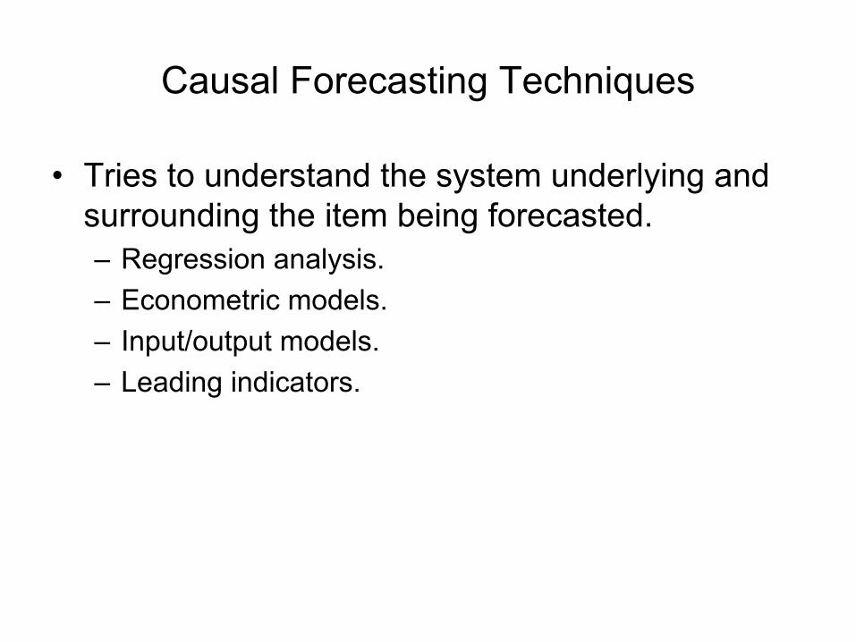
Causal Forecasting Techniques

• Tries to understand the system underlying and surrounding the item being forecasted.– Regression analysis.– Econometric models.– Input/output models.– Leading indicators.

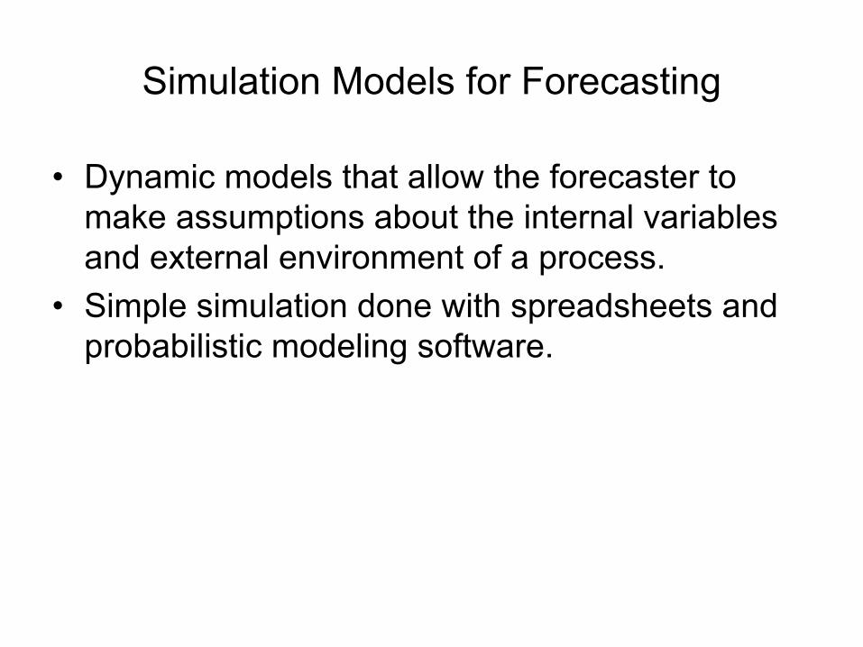
Simulation Models for Forecasting

• Dynamic models that allow the forecaster to make assumptions about the internal variables and external environment of a process.

• Simple simulation done with spreadsheets and probabilistic modeling software.

Which model to use depends on:

• Time horizon to forecast.• Data availability.• Accuracy required.• Size of forecasting budget.• Availability of qualified personnel.

Appropriate Forecasting Methods

Short to mediumStationary, trend, & seasonality

10 to 20 pts. for seasonality

Linear regression

ShortStationary and trend

5 to 10 data points as a minimum

Exponential smoothing w/ trend

ShortStationary, notrends/seasons

5 to 10 data pts.Weighted moving average

Short to mediumStationary, no trend/seasons

6 to 12 weeks,months of data

Simple movingaverage

ForecastHorizon

DataPattern

Amount of Data

ForecastingMethod

Moving Average Techniques

• Simple moving average.– F(t) = [(A(t-1) + A(t-2) + A(t-3))/3] is a three time

period moving average.– If actual demand in March was 20, in February 18,

and in January 16.Forecast (April) = [(20 + 18 + 16)/3] = 54/3 = 18

• Weighted moving average.– F(t) = (w1)(A(t-1)) + (w2)(A(t-2)) + (w3)(A(t-3)) is a

three time period weighted moving average.– Forecast (April) = (0.6)(20) + (0.3)(18) + (0.1)(16) =

18.4

Exponential Smoothing

• Single exponential smoothing.– F(t) = F(t-1) + alpha[A(t-1) – F(t-1)] where alpha

(smoothing constant): 0 <= alpha <= 1.• Exponential smoothing with trend.

– FIT(t) = F(t) + T(t)– F(t) = FIT(t-1) + alpha[A(t-1) – FIT(t-1)]– T(t) = T(t-1) + beta[F(t) - FIT(t-1)] where beta

(smoothing constant): 0 <= beta <= 1.

Linear Regression (Least Squares Method)

• Used both for time series forecasting and for causal relationship forecasting.

• Past data and future projections are assumed to fall about a straight line.

• Linear regression line is the form of Y = a + bXwhere:– Y is the value of the dependent variable.– a is the Y intercept.– b is the slope.– X is the independent variable.

Box-Jenkins and Shiskin Approaches

• Box and Jenkins popularized an approach that combines the moving averages and the autoregressive approaches. Their contribution was developing a systematic methodology for identifying and estimating models that could incorporate both approaches.

• Shiskin developed the business cycles statistics program at the Census Bureau and Census II program for seasonal adjustment of time series.

Sources of Forecast Errors

• Bias errors occur when a consistent mistake is made.– Failure to include right variables.– Use of the wrong relationships among variables.– Employing the wrong trend line.– Mistaken shift in the seasonal demand.

• Random errors are those that cannot be explained by the forecast model being used.

Measurement of Forecast Errors

• Mean Absolute Deviation (MAD).– The average error in the forecast.– Measures dispersion of some observed value from some

expected value.– MAD = sum of the absolute differences of actuals minus

forecasts divided by the number of data pairs.– 1 MAD = 0.8 standard deviation when errors are normally

distributed.

• Tracking Signal (TS).– Indicates whether the forecast is keeping pace with

upward/downward movements in demand.– TS = RSFE/MAD where RSFE is running sum of forecast errors.

• It is important to know when and how to use forecasting.

• It is important to know how to complement forecasting with other methodologies.

• It is important to know and understand how other organizations are using forecasting.

• It is important to keep abreast of new forecasting developments (methods, techniques, software).

Parting Thoughts