This article was downloaded by: [UNSW Library]On: 03 March 2014, At: 15:59Publisher: Taylor & FrancisInforma Ltd Registered in England and Wales Registered Number: 1072954 Registered office: MortimerHouse, 37-41 Mortimer Street, London W1T 3JH, UK

International Journal of Management Science andEngineering ManagementPublication details, including instructions for authors and subscription information:http://www.tandfonline.com/loi/tmse20

Ordering policy in a supply chain with adaptiveneuro-fuzzy inference system demand forecastingHasan Habibul Latifa, Sanjoy Kumar Paula & Abdullahil Azeema

a Department of Industrial and Production Engineering, Bangladesh University ofEngineering and Technology, Dhaka-1000, BangladeshPublished online: 14 Jan 2014.

To cite this article: Hasan Habibul Latif, Sanjoy Kumar Paul & Abdullahil Azeem (2014) Ordering policy in a supply chainwith adaptive neuro-fuzzy inference system demand forecasting, International Journal of Management Science andEngineering Management, 9:2, 114-124, DOI: 10.1080/17509653.2013.866332

To link to this article: http://dx.doi.org/10.1080/17509653.2013.866332

PLEASE SCROLL DOWN FOR ARTICLE

Taylor & Francis makes every effort to ensure the accuracy of all the information (the “Content”) containedin the publications on our platform. However, Taylor & Francis, our agents, and our licensors make norepresentations or warranties whatsoever as to the accuracy, completeness, or suitability for any purpose ofthe Content. Any opinions and views expressed in this publication are the opinions and views of the authors,and are not the views of or endorsed by Taylor & Francis. The accuracy of the Content should not be reliedupon and should be independently verified with primary sources of information. Taylor and Francis shallnot be liable for any losses, actions, claims, proceedings, demands, costs, expenses, damages, and otherliabilities whatsoever or howsoever caused arising directly or indirectly in connection with, in relation to orarising out of the use of the Content.

This article may be used for research, teaching, and private study purposes. Any substantial or systematicreproduction, redistribution, reselling, loan, sub-licensing, systematic supply, or distribution in anyform to anyone is expressly forbidden. Terms & Conditions of access and use can be found at http://www.tandfonline.com/page/terms-and-conditions

Ordering policy in a supply chain with adaptive neuro-fuzzy inferencesystem demand forecasting

Hasan Habibul Latif, Sanjoy Kumar Paul* and Abdullahil Azeem

Department of Industrial and Production Engineering, Bangladesh University of Engineering and Technology, Dhaka-1000, Bangladesh

(Received 26 June 2013; final version received 15 October 2013)

Determining ordering policy has incisive impacts on the success or letdown of an organization. This research has considered

reliability while developing a method for finding ordering policy for multiple supply chain stages through optimal lot sizing.

Setup cost, production cost, inspection cost, rejection cost, interest and depreciation cost, holding cost, etc. are considered

for each supply chain stage whereas the demand inputs in the costs are taken from an adaptive neuro-fuzzy inference system

generated forecasting method. Later, a genetic algorithm has been applied to find the optimum lot size at multiple levels ofsupply chain network to minimize total cost. Optimal lot size, reliability and total cost are determined and the costs are

accumulated to determine total minimum supply chain cost. To validate the model, a comparison with the current situation

clearly indicates the superiority of proposed model over the usual company approach to ordering policy.

Keywords: ordering policy; supply chain; adaptive neuro-fuzzy inference systems; lot size; genetic algorithm; reliability

JEL Classification: C53; C61; C44; C45

1. Introduction

In this era of the competitive market, every kind of

organization goes for unique strategies to grab market

share by fulfilling customer demand. For that purpose,

companies’ objectives are to acquire a persuasive ordering

policy by which their capabilities and efficiencies are

pushed to the limit. Ordering policy is the overall strategy

of an organization by which it can progress the product

according to a predefined way to maintain the organiz-

ation’s overall target. Achieving the appropriate ordering

policy enables minimal supply chain cost as well as

customer satisfaction for an organization. Although it is

difficult to locate every possible factor influencing

ordering policy for an organization, countless methods

have already been identified and more research is ongoing

to define the system of optimal ordering policy. It is a

tradeoff between performance and cost in various stages of

the supply chain while defining ordering policy. Generally,

an ordering policy is defined by respective costs, customer

mindset, the company’s strategic view, product variability,

truck load, product specification, etc. The bullwhip effect,

substantial amounts of unnecessary costs, customer

dissatisfaction, low efficacy, low market penetration, etc.

are the impacts of incorrect ordering policy. So,

maintaining a non-optimized ordering policy is a costly

exercise and thus it is no surprise to find that many

managers regard this as a prime failing.

The economic production quantity (EPQ) model is

used in much research to find the optimal lot size that

minimizes overall supply chain cost. For this reason, the

EPQ model has been widely accepted as a tool for

developing ordering policy for the last three decades.

There are other interrelated factors, such as demand, price,

reliability and uncertainty, that can affect ordering policy.

Uncertainty is incorporated in the model. A myriad of

impediments like abrupt changes in customer demand,

uncertain impacts and seasonal variations could be well

tackled by adaptive neuro-fuzzy inference system

(ANFIS) generated demand forecasting.

In recent years, ANFIS has been successfully applied

to the prediction of water level by Chang and Chang

(2006), weather forecasting (Tektas, 2010), and demand

forecasting (Mahbub, Paul, & Azeem, 2013; Zahin, Latif,

Paul, & Azeem, 2013). Salameh and Jaber (2000) initially

developed the economic order quantity (EOQ) with

imperfect quality. Later on, Goyal and Cardenas-Barron

(2002) presented a straightforward method to find the EPQ

for an item with imperfect quality. Huang and Kuang

(2005) scrutinized replenishment decision policies under

two levels of trade credit policy within the EPQ

framework. Lai, Huang, and Huang (2006) considered

that permissible payment delay by the retailer could be

offered by a supplier when the retailer ordered a sufficient

quantity. Otherwise, permissible delay in payments would

not be permitted. Islam and Roy (2007) proposed an EPQ

model considering the production process and demand

dependent unit production cost with flexibility and

reliability. An integrated production inventory policy

under a finite planning horizon and a linear trend in

demand was presented by Rau and Ouyang (2008). Hejazi,

Tsou, and Rasti Barjoki (2008) proposed an EPQ model

with reduced pricing, rework and reject situations in a

single stage supply chain network in which rework took

place in each cycle after processing. Panda (2013)

coordinated a retail chain with price and time dependent

demand rate which gives a pretty good idea about how a

retail chain behaves with variation of demand and why we

need an algorithm to deal with that problem.

q 2014 International Society of Management Science and Engineering Management

*Corresponding author. Email: sanjoy@ipe.buet.ac.bd

International Journal of Management Science and Engineering Management, 2014

Vol. 9, No. 2, 114–124, http://dx.doi.org/10.1080/17509653.2013.866332

Dow

nloa

ded

by [

UN

SW L

ibra

ry]

at 1

5:59

03

Mar

ch 2

014

Chen and Cheng (2008) adopted a fuzzy economic

production quantity (FEPQ) model with defective pro-

ductions without being repaired. An EPQ model with

deteriorating item which has linearly displayed demand

under inflation and time value of money was presented by

Pal et al. (2009). In that research, it was assumed that

demand is fuzzy in nature for the combined effect of

inflation and the time value ofmoney. A particular case was

also analysed, where the accumulated effect of inflation and

time value were crisp in nature. Total expected profit for the

planning horizon was maximized using a genetic algorithm

(GA) for a crisp inflation effect (Pal et al., 2009). Panda and

Maiti (2009) enlarged a multi-item EPQ model with price,

infinite production rate, dependent demand, stock depen-

dent unit production and holiday costs with the consider-

ation of reliability and flexibility. Hum and Liu (2010)

looked into the optimal replenishment policy under

allowable delay in payments and tolerable shortages within

an EPQ framework. Meanwhile, Seyed and Seyed (2008)

proposed a multi-product EPQ model in which the

existence of defective items in a production were accepted

and reworks were considerable despite of having ware-

house space constraints. Sadjadi, Aryanezhad, and

Jabbazadeh (2010) developed a novel approach where the

reliability of production is incorporated into pricing,

marketing and production planning. Pattnaik (2013) also

modified the widely used EOQ for deterioration in the

presence of imprecise items.

Previous work was mostly focused on optimal lot

ordering policy with constant demand. Process reliability

was ignored in some cases, and multiple supply chain

network stages were also missing. Conventional costs

were usually considered, such as holding cost, production

cost and setup cost. The impacts of non-conventional costs

such as rejection cost and depreciation cost at multiple

levels have not been considered with process reliability

before. Also, previous work has been very sporadic, so a

proper algorithm is required to deal with aspects of the

problem such as the bullwhip effect and shortage of

product. This paper emphasizes meeting customer demand

for any kind of demand pattern, including uncertainty

through ANFIS. To get the broader view and a closer look

at pragmatic problems, a two stage supply chain network

has been considered with respect to customized cost

drivers and reliability for each stage. Later, an attempt has

been made to compare with a pragmatic example to show

the optimized overall ordering policy through a GA on the

basis of total supply chain cost.

2. Problem definition

Well-known variables in supply chain networks are the lot

size of the product and the demand forecast for it. The

success of demand forecasting is dependent on how itworks

with seasonal variation. Lot size also plays a significant

role. Total supply chain cost can be greatly affected by lot

size selection. Organizations and managers are interested

most of the time in, and concerned by, lot sizing. Knowing a

suitable method for approaching demand forecasting and

lot sizing would greatly influence decision making and

improve the overall aggregation of products.

The purpose of the present research is to extend previous

EPQ model research by employing knowledge of forecast-

ing methods, cost of quality, and reliability of production in

multiple supply chain stages. In this research, demand rate

has been derived from the ANFISmodel, where uncertainty

is aggregated. In addition to that, production capacity and

inventory holding cost, setup cost, inspection cost per unit,

and rejection cost per unit of the product are known

parameters, and there are defective items which will be

rejected upon inspection with a reduced price. The selling

price of fresh units is taken as a mark-up over the unit

production cost. The model is formulated to determine

optimal reliability and lot size for a multiple stage supply

chain in order to minimize total supply chain cost.

Mathematically, equations are obtained and derived for

production cost, holding cost, setup cost, inspection cost,

rejection cost, cost of interest and depreciation with

reliability of the productionprocess,which is very important

in real life production inventory problems. As a result, the

inventory model in this paper is more practical than the

traditional EPQ model. A GA has been used to deduce the

optimal lot size, as it can generate more accurate results

within a shorter computer time than any other method.

3. Assumptions and notation

Some assumptions are made in this research. These are as

follows.

(1) The demand rate is variable and derived from ANFIS.

(2) There are defective items in the production. All items

are inspected.

(3) There are at least two stages available in the supply

chain network.

(4) Lot size (Q) and process reliability (R) are decision

variables.

(5) Production rate is similar to the demand. Extra

production is not desirable.

(6) Demand is considered as retailer end demand. The

same demand is used for distributor end demand.

(7) The total cost of interest and depreciation per

production cycle is dependent on setup cost (S) and

reliability (R) as proposed by Seyed and Seyed

(2008):

TðR; S;HÞ ¼ RdS2eH2f ; ð1Þ

where, d, e and f are reliability, setup cost and holding cost

elasticity, respectively, to provide the best fit to the

estimated cost function.

The notation of the model is given as follows.

D ¼ Demand per cycle time

R ¼ Production reliability

Q ¼ Lot size

C ¼ Production cost per unit

International Journal of Management Science and Engineering Management 115

Dow

nloa

ded

by [

UN

SW L

ibra

ry]

at 1

5:59

03

Mar

ch 2

014

S ¼ Setup cost per cycle

D ¼ Holding cost per unit per cycle time

d ¼ Reliability elasticity; 0 # d # 1

e ¼ Setup cost elasticity; 0 # e # 1

f ¼ Holding cost elasticity; 0 # f # 1

t ¼ Cycle time

I ¼ Inspection cost per unit

J ¼ Rejection cost per unit

T(R,S,H) ¼ Depreciation and interest cost

4. Solution approach

In this study, a new model is developed that incorporates

the reliability as part of an integrated model. The model

simultaneously determines the lot size (Q) and production

reliability (R). Demand is generated from the ANFIS

model, which greatly mitigates the uncertainty of demand

variation. The total cost incurred in a production cycle is

the sum of different corresponding costs for different

stages. Finally, a genetic algorithm is used to find the best

suited lot size and process reliability.

The reason for using a genetic algorithm is that it

allows the computer to compute. It goes through the

maximum possible number of combinations within a short

space of time, which is beyond human capacity. For

combinational optimization problems, genetic algorithms

have a clear edge over some other techniques such as

particle swarm optimization and ant colony techniques.

Though it does not provide global optimality of the

solution, its quick response and intense operation method

makes the genetic algorithm a better fit for the model.

4.1. Generation of demand data from ANFIS

Using the ANFIS model, demand data have been

generated from collected retailer end demand data.

Various factors that influence the uses of the product

have been considered. After considering all these factors,

demand data has been generated that will be used in the

solution approach according to the algorithm depicted

below. A dataset has to be generated wherein the variation

of inputs will be reflected in the significance of the outputs.

The appropriateness of the dataset should be acute and

handled with deliberation. The relationship between

several inputs is not always easy to identify. Moreover,

uncertainty and noise will always incorporated in the

dataset. Thus, ANFIS could forecast demand data well

with its efficiency for incorporating uncertainty.

4.2. Setting the objective function

(1) Production cost

Tripathy, Wee, and Majhi (2003) have proposed

that the unit cost of production is related to reliability

proportionally, and inversely related to demand after

exceeding supply. Again, Tripathy and Pattnaik (2009)

said that the unit cost of production behaves inversely

with process reliability and demand. Denoting C as the

unit production cost, the total production cost is CD.

If reliability is involved, the equation will be changed.

Due to increased reliability, production cost will

increase because of producing D/R products instead of

the regular demand D. So, it is clear that the total

production cost is inversely related to the reliability of

the production process:

Total production cost ¼ CD

R: ð2Þ

(2) Setup cost

Setup cost refers to expenses incurred each time a

batch is produced. It consists of the engineering cost of

setting up the production runs or machines, the

paperwork cost of processing thework order, the ordering

cost to provide raw materials for batch processing, etc. S

is the setup cost per cycle and t is the cycle time or

production period in each cycle. In traditional EPQ and

EOQ models, cycle time t is represented as QR/D. If

reliability is incorporated with setup cost,

Total setup cost ¼ DS

QR: ð3Þ

(3) Holding cost

The holding cost is associated with keeping

inventory, including warehousing, spoilage, obsoles-

cence, interest and taxes. It is also called the inventory

carrying cost. The inventory holding cost per cycle is

obtained as the average inventory multipied by the

holdingcost perproduct per cycle.As theaverage amount

of inventory held each year is Q/2R the reliability

incorporated holding cost would be as follows:

Holding cost ¼ QH

2R: ð4Þ

(4) Depreciation and interest cost

Seyed and Seyed (2008) proposed adding deprecia-

tion and interest cost to the framework.An increase in the

reliability of the production process thus leads to growth

in the total interest and depreciation cost. High reliability

can be achieved with additional cost in practice. So, the

total cost of interest anddepreciation per productioncycle

is assumed to be a function of reliability and setup cost:

Depreciation and interest cost ¼ TðR; S;HÞ¼ RdS2eH2f : ð5Þ

(5) Inspection cost

Hejazi et al. (2008) have determined the economic

production quantity with reduced pricing, rework and

reject situations in a single stage system in which rework

takes places in each cycle after processing to minimize

total system costs. A mathematical model is developed

and numerical examples are presented to illustrate the

usefulness of thismodel.A100%inspection is performed

in order to identify the number of good quality items,

H.H. Latif et al.116

Dow

nloa

ded

by [

UN

SW L

ibra

ry]

at 1

5:59

03

Mar

ch 2

014

imperfect items and defective items in each lot. It is

assumed that inspection only takes place during

processing time. If I is the per unit inspection cost, then

Inspection cost ¼ D2

QIR: ð6Þ

(6) Rejection cost

Hejazi et al. (2008) have also considered rejection

cost in their proposed model. This paper considers a

reduced price for selling the defective items without any

delay. If the process reliability is R, then (1 2 R)% of the

product is defective. If the cost of the defective product is

J then the rejection cost per unit time can be derived as

Rejection cost ¼ ð12 RÞD2

QJ: ð7Þ

So the equation for the total cost stands as

Total Cost ¼ ðProduction costþ Setup cost

þ Holding costþ Inspection cost

þ Rejection cost

þ Interest and depreciation costÞ:Using Equations (2)–(7), the total cost per cycle is

obtained as

Total cost per cycle ¼CD

Rþ DS

QRþ QH

2Rþ D 2

QIR

þ ð12 RÞD2

QJ þ RdS2eH2f :

ð8Þ

The objective is to minimize the total cost per cycle

subject to the constraint that process reliability cannot

exceed 100%. The model is unconstrained non-integer and

nonlinear in nature, such that reaching an analytic solution

to the problem is difficult. ANFIS helped to derive the

demand per cycle time, which is ultimately used as a

constant. Later, the GA is used to decide the optimal

solution for different stages of the supply chain. The costs

must be considered independently with respect to that

particular stage. The number of cost considerations will

vary according to the supply chain stage. Finally, the study

analyses the behavior of themodel using a realistic example

and compares the results on the same inventory model.

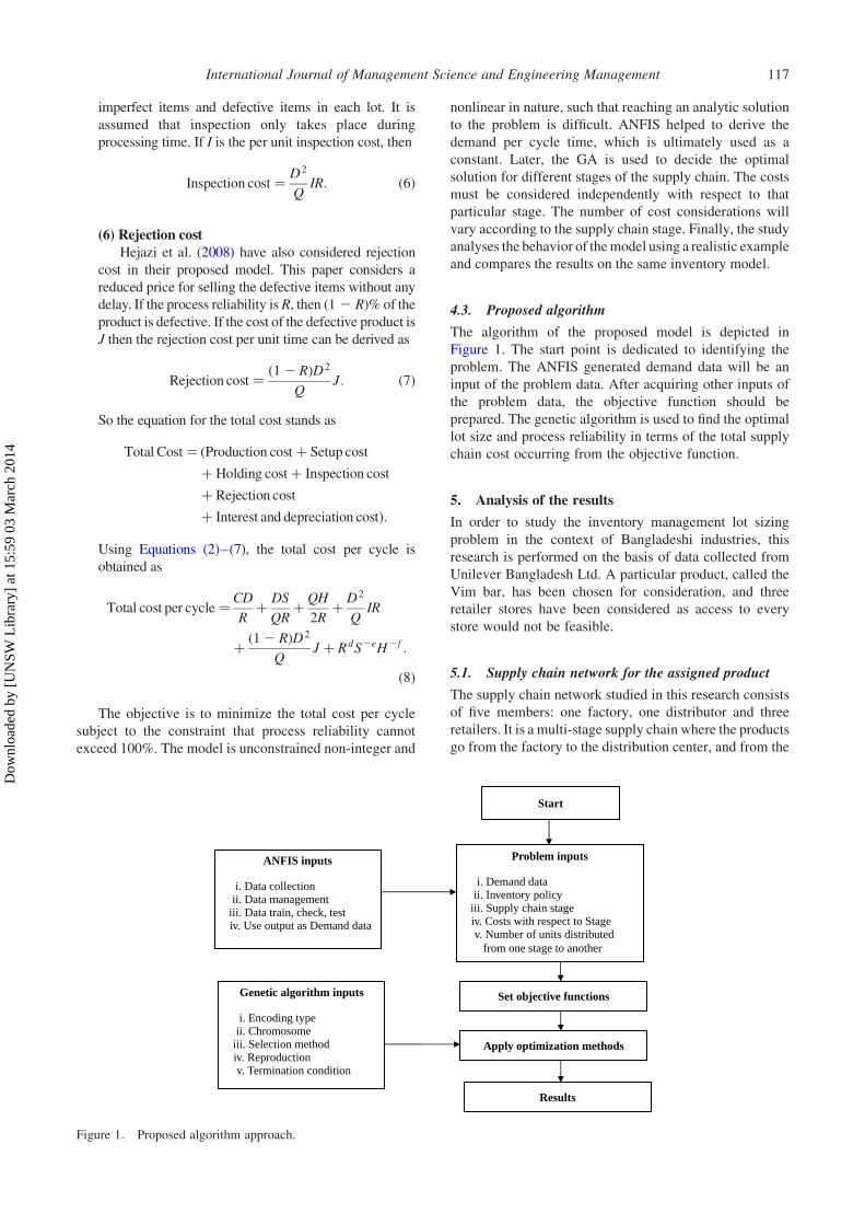
4.3. Proposed algorithm

The algorithm of the proposed model is depicted in

Figure 1. The start point is dedicated to identifying the

problem. The ANFIS generated demand data will be an

input of the problem data. After acquiring other inputs of

the problem data, the objective function should be

prepared. The genetic algorithm is used to find the optimal

lot size and process reliability in terms of the total supply

chain cost occurring from the objective function.

5. Analysis of the results

In order to study the inventory management lot sizing

problem in the context of Bangladeshi industries, this

research is performed on the basis of data collected from

Unilever Bangladesh Ltd. A particular product, called the

Vim bar, has been chosen for consideration, and three

retailer stores have been considered as access to every

store would not be feasible.

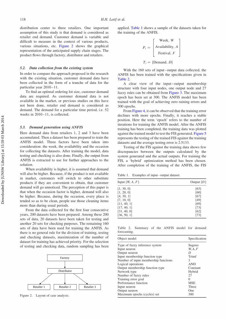
5.1. Supply chain network for the assigned product

The supply chain network studied in this research consists

of five members: one factory, one distributor and three

retailers. It is a multi-stage supply chain where the products

go from the factory to the distribution center, and from the

Start

Problem inputs

i. Demand dataii. Inventory policy

iii. Supply chain stageiv. Costs with respect to Stagev. Number of units distributed from one stage to another

ANFIS inputs

i. Data collectionii. Data management

iii. Data train, check, testiv. Use output as Demand data

Set objective functions

Apply optimization methods

Genetic algorithm inputs

i. Encoding typeii. Chromosome

iii. Selection methodiv. Reproductionv. Termination condition

Results

Figure 1. Proposed algorithm approach.

International Journal of Management Science and Engineering Management 117

Dow

nloa

ded

by [

UN

SW L

ibra

ry]

at 1

5:59

03

Mar

ch 2

014

distribution center to three retailers. One important

assumption of this study is that demand is considered as

retailer end demand. Customer demand is variable and

difficult to measure in the context of various products,

various situations, etc. Figure 2 shows the graphical

representation of the anticipated supply chain stages. The

product flows through factory, distributor and retailers.

5.2. Data collection from the existing system

In order to compare the approach proposed in the research

with the existing situation, customer demand data have

been collected in the form of a tranche of data for the

particular year 2010–11.

To find an optimal ordering lot size, customer demand

data are required. As customer demand data is not

available in the market, or previous studies on this have

not been done, retailer end demand is considered as

demand. The demand for a particular time period, i.e. 52

weeks in 2010–11, is collected.

5.3. Demand generation using ANFIS

Here demand data from retailers 1, 2 and 3 have been

accumulated. Then a dataset has been prepared to train the

ANFIS model. Three factors have been taken into

consideration: the week, the availability and the occasion

for collecting the datasets. After training the model, data

testing and checking is also done. Finally, the output from

ANFIS is extracted to use for further approaches to the

solution.

When availability is higher, it is assumed that demand

will also be higher. Because, if the product is not available

in market, customers will switch to other substitute

products if they are convenient to obtain, that customer

demand will go unnoticed. The perception of this paper is

that when the occasion factor is higher, demand will also

be higher. Because, during the occasion, every place is

tended so as to be clean, people use those cleaning items

more than during usual periods.

From the data collected for the first four consecutive

years, 200 datasets have been prepared. Among these 200

sets of data, 20 datasets have been taken for testing and

another 20 sets for checking purposes. The remaining 160

sets of data have been used for training the ANFIS. As

there is no general rule for the division of training, testing

and checking datasets, maximization of the number of

dataset for training has achieved priority. For the selection

of testing and checking data, random sampling has been

applied. Table 1 shows a sample of the datasets taken for

the training of the ANFIS.

Pi ¼Week; W

Availability; A

Festival; F

2664

3775

Ti ¼ ½Demand; D�With the 160 sets of input–output data collected, the

ANFIS has been trained with the specifications given in

Table 2.

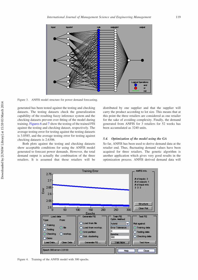
A clear view of the input–output membership

structure with four input nodes, one output node and 27

fuzzy rules can be obtained from Figure 3. The maximum

epoch has been set at 300. The ANFIS model has been

trained with the goal of achieving zero raining errors and

300 epochs.

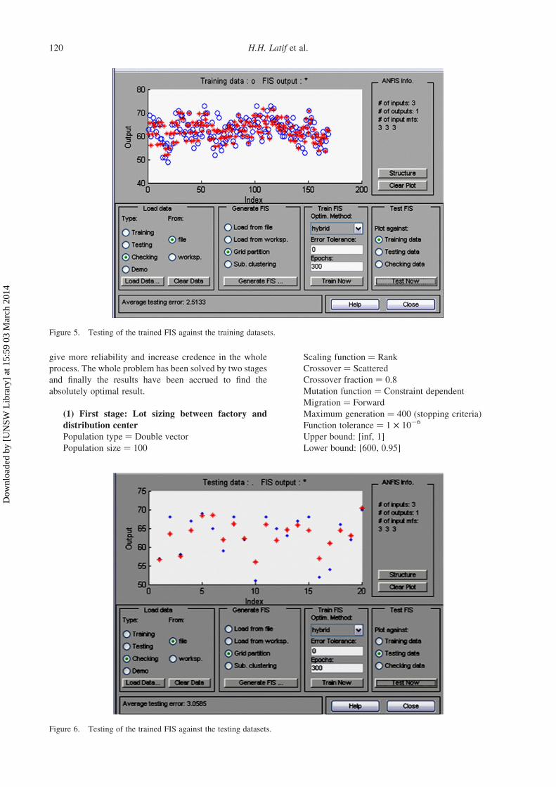
From Figure 4, it can be observed that the training error

declines with more epochs. Finally, it reaches a stable

position. Here the term ‘epoch’ refers to the number of

iterations for training the ANFIS model. After the ANFIS

training has been completed, the training data was plotted

against the trained model to test the FIS generated. Figure 5

represents the testing of the trained FIS against the training

datasets and the average testing error is 2.5133.

Testing of the FIS against the training data shows few

discrepancies between the outputs calculated by the

system generated and the actual outputs. For training the

FIS, a ‘hybrid’ optimization method has been chosen.

After completion of the training of the ANFIS, the FIS

Factory

Distributor

Retailer 1 Retailer 2 Retailer 3

Figure 2. Layout of case analysis.

Table 2. Summary of the ANFIS model for demandforecasting.

Object model Specification

Type of fuzzy inference system SugenoInput neuron W,A,FOutput neuron DInput membership function type TrimfNumber of input membership functions 3Logical operations ANDOutput membership function type ConstantNetwork type HybridNumber of fuzzy rules 27Training error goal 0Performance function MSEInput neuron ThreeOutput neuron OneMaximum epochs (cycles) set 300

Table 1. Examples of input–output dataset.

Input [W, A, F ] Output [D ]

[1, 30, 0] [63][1, 20, 0] [60][4, 30, 1] [67][7, 10, 0] [49][11, 40, 1] [69][17, 40, 1] [73][31, 40, 0] [62][36, 50, 1] [73]

H.H. Latif et al.118

Dow

nloa

ded

by [

UN

SW L

ibra

ry]

at 1

5:59

03

Mar

ch 2

014

generated has been tested against the testing and checking

datasets. The testing datasets check the generalization

capability of the resulting fuzzy inference system and the

checking datasets prevent over fitting of the model during

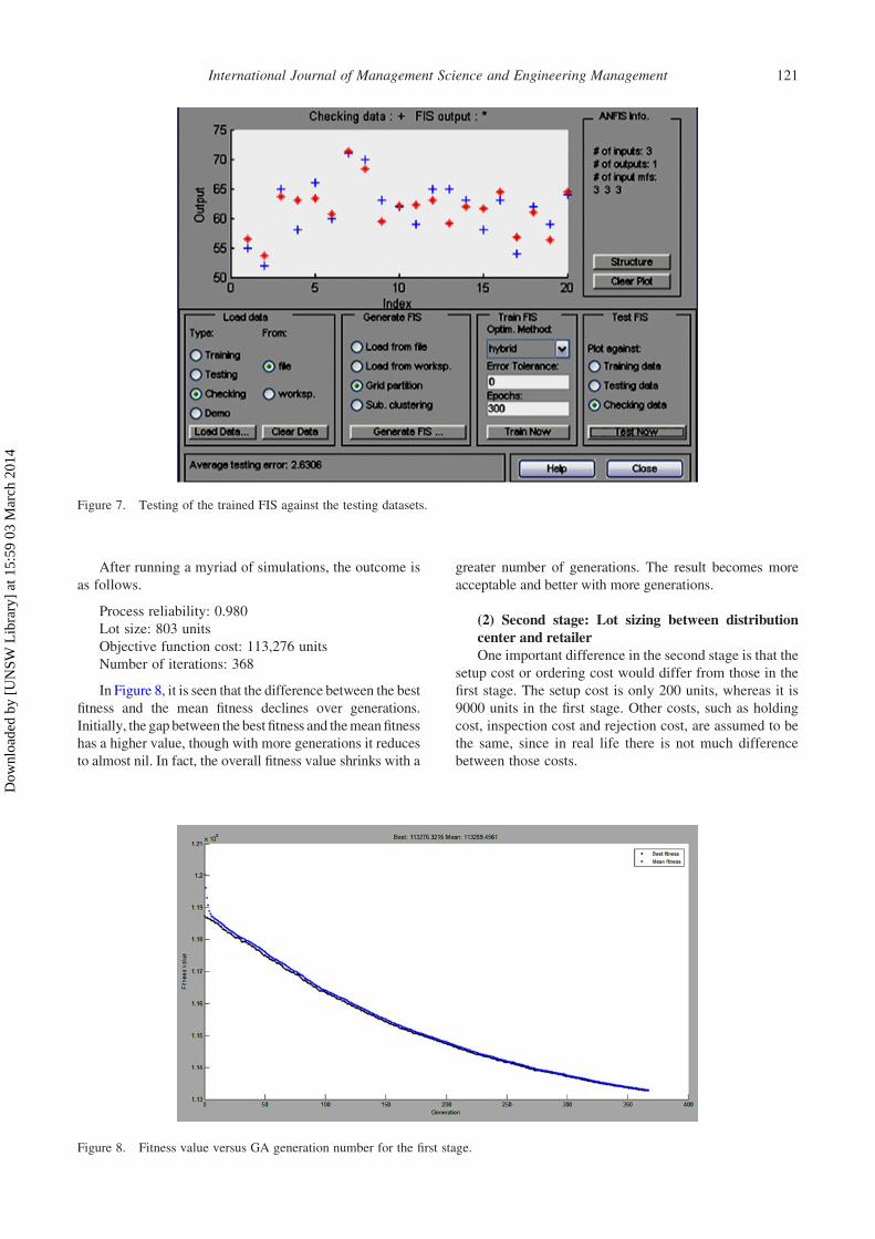
training. Figures 6 and 7 show the testing of the trained FIS

against the testing and checking dataset, respectively. The

average testing error for testing against the testing datasets

is 3.0585, and the average testing error for testing against

checking datasets is 2.6306.

Both plots against the testing and checking datasets

show acceptable conditions for using the ANFIS model

generated to forecast power demands. However, the total

demand output is actually the combination of the three

retailers. It is assumed that those retailers will be

distributed by one supplier and that the supplier will

carry the product according to lot size. This means that at

this point the three retailers are considered as one retailer

for the sake of avoiding complexity. Finally, the demand

generated from ANFIS for 3 retailers for 52 weeks has

been accumulated as 3240 units.

5.4. Optimization of the model using the GA

So far, ANFIS has been used to derive demand data at the

retailer end. Thus, fluctuating demand values have been

acquired for three retailers. The genetic algorithm is

another application which gives very good results in the

optimization process. ANFIS derived demand data will

Figure 3. ANFIS model structure for power demand forecasting.

Figure 4. Training of the ANFIS model with 300 epochs.

International Journal of Management Science and Engineering Management 119

Dow

nloa

ded

by [

UN

SW L

ibra

ry]

at 1

5:59

03

Mar

ch 2

014

give more reliability and increase credence in the whole

process. The whole problem has been solved by two stages

and finally the results have been accrued to find the

absolutely optimal result.

(1) First stage: Lot sizing between factory and

distribution center

Population type ¼ Double vector

Population size ¼ 100

Scaling function ¼ Rank

Crossover ¼ Scattered

Crossover fraction ¼ 0.8

Mutation function ¼ Constraint dependent

Migration ¼ Forward

Maximum generation ¼ 400 (stopping criteria)

Function tolerance ¼ 1 £ 1026

Upper bound: [inf, 1]

Lower bound: [600, 0.95]

Figure 5. Testing of the trained FIS against the training datasets.

Figure 6. Testing of the trained FIS against the testing datasets.

H.H. Latif et al.120

Dow

nloa

ded

by [

UN

SW L

ibra

ry]

at 1

5:59

03

Mar

ch 2

014

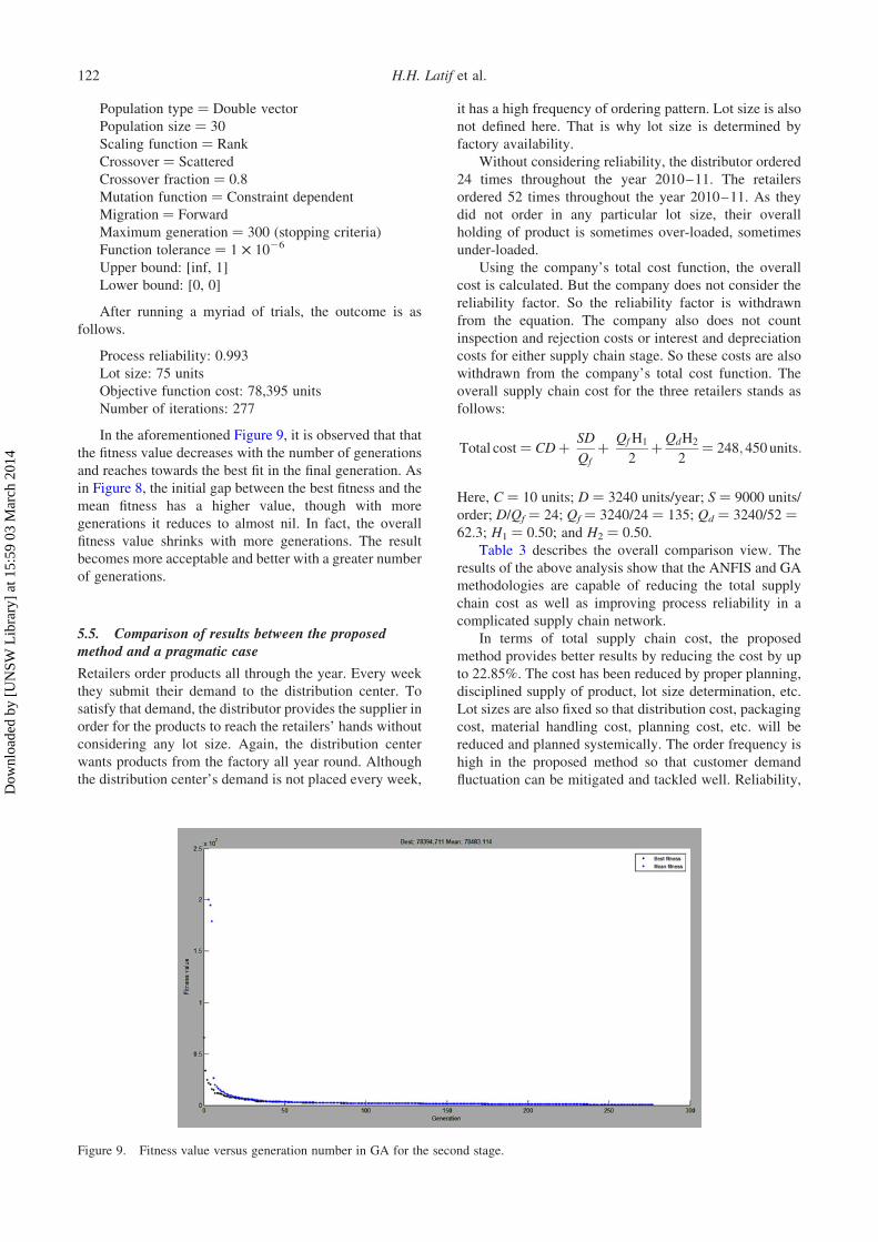
After running a myriad of simulations, the outcome is

as follows.

Process reliability: 0.980

Lot size: 803 units

Objective function cost: 113,276 units

Number of iterations: 368

In Figure 8, it is seen that the difference between the best

fitness and the mean fitness declines over generations.

Initially, the gap between the best fitness and themeanfitness

has a higher value, though with more generations it reduces

to almost nil. In fact, the overall fitness value shrinks with a

greater number of generations. The result becomes more

acceptable and better with more generations.

(2) Second stage: Lot sizing between distribution

center and retailer

One important difference in the second stage is that the

setup cost or ordering cost would differ from those in the

first stage. The setup cost is only 200 units, whereas it is

9000 units in the first stage. Other costs, such as holding

cost, inspection cost and rejection cost, are assumed to be

the same, since in real life there is not much difference

between those costs.

Figure 7. Testing of the trained FIS against the testing datasets.

Figure 8. Fitness value versus GA generation number for the first stage.

International Journal of Management Science and Engineering Management 121

Dow

nloa

ded

by [

UN

SW L

ibra

ry]

at 1

5:59

03

Mar

ch 2

014

Population type ¼ Double vector

Population size ¼ 30

Scaling function ¼ Rank

Crossover ¼ Scattered

Crossover fraction ¼ 0.8

Mutation function ¼ Constraint dependent

Migration ¼ Forward

Maximum generation ¼ 300 (stopping criteria)

Function tolerance ¼ 1 £ 1026

Upper bound: [inf, 1]

Lower bound: [0, 0]

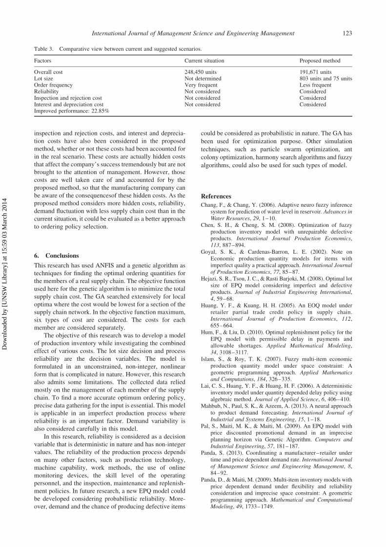
After running a myriad of trials, the outcome is as

follows.

Process reliability: 0.993

Lot size: 75 units

Objective function cost: 78,395 units

Number of iterations: 277

In the aforementioned Figure 9, it is observed that that

the fitness value decreases with the number of generations

and reaches towards the best fit in the final generation. As

in Figure 8, the initial gap between the best fitness and the

mean fitness has a higher value, though with more

generations it reduces to almost nil. In fact, the overall

fitness value shrinks with more generations. The result

becomes more acceptable and better with a greater number

of generations.

5.5. Comparison of results between the proposedmethod and a pragmatic case

Retailers order products all through the year. Every week

they submit their demand to the distribution center. To

satisfy that demand, the distributor provides the supplier in

order for the products to reach the retailers’ hands without

considering any lot size. Again, the distribution center

wants products from the factory all year round. Although

the distribution center’s demand is not placed every week,

it has a high frequency of ordering pattern. Lot size is also

not defined here. That is why lot size is determined by

factory availability.

Without considering reliability, the distributor ordered

24 times throughout the year 2010–11. The retailers

ordered 52 times throughout the year 2010–11. As they

did not order in any particular lot size, their overall

holding of product is sometimes over-loaded, sometimes

under-loaded.

Using the company’s total cost function, the overall

cost is calculated. But the company does not consider the

reliability factor. So the reliability factor is withdrawn

from the equation. The company also does not count

inspection and rejection costs or interest and depreciation

costs for either supply chain stage. So these costs are also

withdrawn from the company’s total cost function. The

overall supply chain cost for the three retailers stands as

follows:

Total cost ¼ CDþ SD

Qf

þ QfH1

2þQdH2

2¼ 248;450units:

Here, C ¼ 10 units; D ¼ 3240 units/year; S ¼ 9000 units/

order; D/Qf ¼ 24; Qf ¼ 3240/24 ¼ 135; Qd ¼ 3240/52 ¼62.3; H1 ¼ 0.50; and H2 ¼ 0.50.

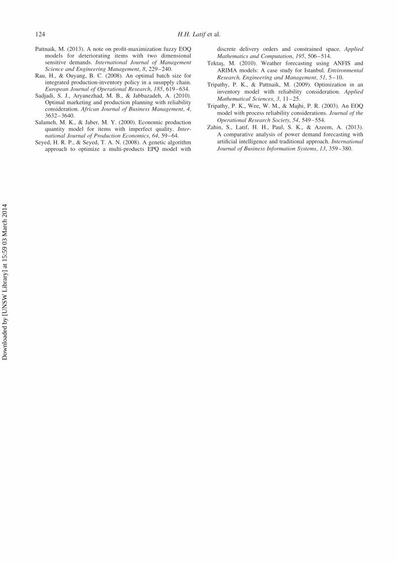
Table 3 describes the overall comparison view. The

results of the above analysis show that the ANFIS and GA

methodologies are capable of reducing the total supply

chain cost as well as improving process reliability in a

complicated supply chain network.

In terms of total supply chain cost, the proposed

method provides better results by reducing the cost by up

to 22.85%. The cost has been reduced by proper planning,

disciplined supply of product, lot size determination, etc.

Lot sizes are also fixed so that distribution cost, packaging

cost, material handling cost, planning cost, etc. will be

reduced and planned systemically. The order frequency is

high in the proposed method so that customer demand

fluctuation can be mitigated and tackled well. Reliability,

Figure 9. Fitness value versus generation number in GA for the second stage.

H.H. Latif et al.122

Dow

nloa

ded

by [

UN

SW L

ibra

ry]

at 1

5:59

03

Mar

ch 2

014

inspection and rejection costs, and interest and deprecia-

tion costs have also been considered in the proposed

method, whether or not these costs had been accounted for

in the real scenario. These costs are actually hidden costs

that affect the company’s success tremendously but are not

brought to the attention of management. However, those

costs are well taken care of and accounted for by the

proposed method, so that the manufacturing company can

be aware of the consequencesof these hidden costs. As the

proposed method considers more hidden costs, reliability,

demand fluctuation with less supply chain cost than in the

current situation, it could be evaluated as a better approach

to ordering policy selection.

6. Conclusions

This research has used ANFIS and a genetic algorithm as

techniques for finding the optimal ordering quantities for

the members of a real supply chain. The objective function

used here for the genetic algorithm is to minimize the total

supply chain cost. The GA searched extensively for local

optima where the cost would be lowest for a section of the

supply chain network. In the objective function maximum,

six types of cost are considered. The costs for each

member are considered separately.

The objective of this research was to develop a model

of production inventory while investigating the combined

effect of various costs. The lot size decision and process

reliability are the decision variables. The model is

formulated in an unconstrained, non-integer, nonlinear

form that is complicated in nature. However, this research

also admits some limitations. The collected data relied

mostly on the management of each member of the supply

chain. To find a more accurate optimum ordering policy,

precise data gathering for the input is essential. This model

is applicable in an imperfect production process where

reliability is an important factor. Demand variability is

also considered carefully in this model.

In this research, reliability is considered as a decision

variable that is deterministic in nature and has non-integer

values. The reliability of the production process depends

on many other factors, such as production technology,

machine capability, work methods, the use of online

monitoring devices, the skill level of the operating

personnel, and the inspection, maintenance and replenish-

ment policies. In future research, a new EPQ model could

be developed considering probabilistic reliability. More-

over, demand and the chance of producing defective items

could be considered as probabilistic in nature. The GA has

been used for optimization purpose. Other simulation

techniques, such as particle swarm optimization, ant

colony optimization, harmony search algorithms and fuzzy

algorithms, could also be used for such types of model.

References

Chang, F., & Chang, Y. (2006). Adaptive neuro fuzzy inferencesystem for prediction of water level in reservoir. Advances inWater Resources, 29, 1–10.

Chen, S. H., & Cheng, S. M. (2008). Optimization of fuzzyproduction inventory model with unrepairable defectiveproducts. International Journal Production Economics,113, 887–894.

Goyal, S. K., & Cardenas-Barron, L. E. (2002). Note onEconomic production quantity models for items withimperfect quality a practical approach. International Journalof Production Economics, 77, 85–87.

Hejazi, S. R., Tsou, J. C., & Rasti Barjoki, M. (2008). Optimal lotsize of EPQ model considering imperfect and defectiveproducts. Journal of Industrial Engineering International,4, 59–68.

Huang, Y. F., & Kuang, H. H. (2005). An EOQ model underretailer partial trade credit policy in supply chain.International Journal of Production Economics, 112,655–664.

Hum, F., & Liu, D. (2010). Optimal replenishment policy for theEPQ model with permissible delay in payments andallowable shortages. Applied Mathematical Modeling,34, 3108–3117.

Islam, S., & Roy, T. K. (2007). Fuzzy multi-item economicproduction quantity model under space constraint: Ageometric programming approach. Applied Mathematicsand Computations, 184, 326–335.

Lai, C. S., Huang, Y. F., & Huang, H. F. (2006). A deterministicinventory model under quantity depended delay policy usingalgebraic method. Journal of Applied Science, 6, 406–410.

Mahbub, N., Paul, S. K., & Azeem, A. (2013). A neural approachto product demand forecasting. International Journal ofIndustrial and Systems Engineering, 15, 1–18.

Pal, S., Maiti, M. K., & Maiti, M. (2009). An EPQ model withprice discounted promotional demand in an impreciseplanning horizon via Genetic Algorithm. Computers andIndustrial Engineering, 57, 181–187.

Panda, S. (2013). Coordinating a manufacturer–retailer undertime and price dependent demand rate. International Journalof Management Science and Engineering Management, 8,84–92.

Panda, D., & Maiti, M. (2009). Multi-item inventory models withprice dependent demand under flexibility and reliabilityconsideration and imprecise space constraint: A geometricprogramming approach. Mathematical and ComputationalModeling, 49, 1733–1749.

Table 3. Comparative view between current and suggested scenarios.

Factors Current situation Proposed method

Overall cost 248,450 units 191,671 unitsLot size Not determined 803 units and 75 unitsOrder frequency Very frequent Less frequentReliability Not considered ConsideredInspection and rejection cost Not considered ConsideredInterest and depreciation cost Not considered ConsideredImproved performance: 22.85%

International Journal of Management Science and Engineering Management 123

Dow

nloa

ded

by [

UN

SW L

ibra

ry]

at 1

5:59

03

Mar

ch 2

014

Pattnaik, M. (2013). A note on profit-maximization fuzzy EOQmodels for deteriorating items with two dimensionalsensitive demands. International Journal of ManagementScience and Engineering Management, 8, 229–240.

Rau, H., & Ouyang, B. C. (2008). An optimal batch size forintegrated production-inventory policy in a susupply chain.European Journal of Operational Research, 185, 619–634.

Sadjadi, S. J., Aryanezhad, M. B., & Jabbazadeh, A. (2010).Optimal marketing and production planning with reliabilityconsideration. African Journal of Business Management, 4,3632–3640.

Salameh, M. K., & Jaber, M. Y. (2000). Economic productionquantity model for items with imperfect quality. Inter-national Journal of Production Economics, 64, 59–64.

Seyed, H. R. P., & Seyed, T. A. N. (2008). A genetic algorithmapproach to optimize a multi-products EPQ model with

discrete delivery orders and constrained space. Applied

Mathematics and Computation, 195, 506–514.

Tektas, M. (2010). Weather forecasting using ANFIS and

ARIMA models: A case study for Istanbul. Environmental

Research, Engineering and Management, 51, 5–10.

Tripathy, P. K., & Pattnaik, M. (2009). Optimization in an

inventory model with reliability consideration. Applied

Mathematical Sciences, 3, 11–25.

Tripathy, P. K., Wee, W. M., & Majhi, P. R. (2003). An EOQ

model with process reliability considerations. Journal of the

Operational Research Society, 54, 549–554.

Zahin, S., Latif, H. H., Paul, S. K., & Azeem, A. (2013).

A comparative analysis of power demand forecasting with

artificial intelligence and traditional approach. International

Journal of Business Information Systems, 13, 359–380.

H.H. Latif et al.124

Dow

nloa

ded

by [

UN

SW L

ibra

ry]

at 1

5:59

03

Mar

ch 2

014