ORIGINAL PAPER

An adaptive neuro-fuzzy inference system for predictingunconfined compressive strength and Young’s modulus:a study on Main Range granite

Danial Jahed Armaghani • Edy Tonnizam Mohamad •

Ehsan Momeni • Mogana Sundaram Narayanasamy •

Mohd For Mohd Amin

Received: 18 June 2014 / Accepted: 7 October 2014

� Springer-Verlag Berlin Heidelberg 2014

Abstract Engineering properties of rocks such as

unconfined compressive strength (UCS) and Young’s

modulus (E) are among the essential parameters for the

design of tunnel excavations. Many attempts have been

made to develop indirect methods of estimating UCS and

E. This is generally attributed to the difficulty of preparing

and conducting the aforementioned tests in a laboratory. In

essence, this study aims to present two predictive models of

UCS and E for granite using an adaptive neuro-fuzzy

inference system (ANFIS). The required rock samples for

model development (45 granite sample sets) were obtained

from site investigation work at the Pahang-Selangor raw

water transfer tunnel, which was excavated across the Main

Range of Peninsular Malaysia. In developing the predictive

models, dry density, ultrasonic velocity, quartz content and

plagioclase were set as model inputs. These parameters

were selected based on simple and multiple regression

analyses presented in the article. However, for the sake of

comparison, the prediction performances of the ANFIS

models were checked against multiple regression analysis

(MRA) and artificial neural network (ANN) predictive

models of UCS and E. The capacity performances of the

predictive models were assessed based on the value

account for (VAF), root mean squared error (RMSE) and

coefficient of determination (R2). It was found that the

ANFIS predictive model of UCS, with R2, RMSE and VAF

equal to 0.985, 6.224 and 98.455 %, respectively, outper-

forms the MRA and ANN models. A similar conclusion

was drawn for the ANFIS predictive model of E where the

values of R2, RMSE and VAF were 0.990, 3.503 and

98.968 %, respectively.

Keywords Unconfined compressive strength � Young’s

modulus � Adaptive neuro-fuzzy inference system �Multiple regression analysis � Granite

Introduction

Proper determination of unconfined compressive strength

(UCS) and Young’s modulus (E) of rocks is of crucial

importance in the design of geotechnical engineering

structures such as dams and tunnels. The latter is a key

parameter in deformation analysis and the former gives

good estimation of the rock bearing capacity. In other

words, inappropriate estimation of the aforementioned rock

parameters, i.e. UCS and E, could be catastrophic as it can

lead to underestimation of the ultimate bearing capacity as

well as the load corresponding to an allowable settlement

for a problem of interest. The unconfined compression test

is a laboratory test normally used to determine elastic

modulus and strength of the rock. The test is conducted

using standard procedures such as those of the International

Society for Rock Mechanics (ISRM). However, there are

D. Jahed Armaghani (&) � E. Tonnizam Mohamad �E. Momeni � M. F. Mohd Amin

Department of Geotechnics and Transportation, Faculty of Civil

Engineering, Universiti Teknologi Malaysia (UTM),

81310 Skudai, Johor, Malaysia

e-mail: danialarmaghani@yahoo.com

E. Tonnizam Mohamad

e-mail: edy@utm.my

E. Momeni

e-mail: mehsan23@live.utm.my

M. F. Mohd Amin

e-mail: mohdfor@utm.my

M. S. Narayanasamy

Aurecon Pty Ltd, Brisbane, Australia

e-mail: mogana.sundaram@aurecongroup.com

123

Bull Eng Geol Environ

DOI 10.1007/s10064-014-0687-4

some impeding factors in direct determination of UCS and

E in the laboratory. For instance, preparing the required

rock core samples is often difficult, especially for rocks

that are highly fractured and those that exhibit significant

lamination and foliation (Singh et al. 2012; Monjezi et al.

2012). At preliminary design stage, direct determination of

UCS and E can be too expensive and time consuming

(Yilmaz and Sendir 2002; Gokceoglu and Zorlu 2004;

Kahraman 2014). Nevertheless, alternative and indirect

approaches of predicting the rock strength and modulus are

available, such as traditional and multiple regression

models and soft computing techniques.

Many attempts have been made in developing conven-

tional (also called indirect) methods of UCS or E estima-

tion. These alternative methods for predicting UCS and E,

are often in forms of simple regression between UCS or

E and simple index tests of rocks such as the Schmidt

hammer (Singh et al. 1983; Yasar and Erdogan 2004; Nazir

et al. 2013b; Karaman and Kesimal 2014), ultrasonic

velocity, or Vp (Kahraman 2001; Cobanglu and Celik

2008), Brazilian tensile strength (Gokceoglu and Zorlu

2004; Kahraman et al. 2012; Nazir et al. 2013a), point-load

index (Sulukcu and Ulusay 2001; Basu and Aydin 2006;

Tandon and Gupta 2014) and slake durability index

(Moradian et al. 2010; Yagiz 2011) tests.

In addition, some researchers addressed the successful

application of multiple regression analysis (MRA) in pre-

dicting rock strength and module of elasticity (Gokceoglu

and Zorlu 2004; Yilmaz and Yuksek 2009). However, there

are some reported cases where these correlations are found

to be insufficient to provide highly reliable values of the

UCS and E (Dehghan et al. 2010; Beiki et al. 2013). In

general, the use of these equations is recommended only

for specific rock types (Beiki et al. 2013). Furthermore,

statistical prediction methods suffer from a disadvantage in

respect to new available data: If different from the original

data, the form of the obtained equations needs to be

updated (O’Rourke 1989; Rezaei et al. 2012).

Recent studies have highlighted the application of soft

computation techniques such as the artificial neural net-

work (ANN) and the adaptive neuro-fuzzy inference sys-

tem (ANFIS) in geotechnical engineering problems. This is

attributed to the well-established fact that soft computation

techniques are feasible, quick and promising tools for the

solving of engineering problems, particularly when the

contact natures between independent variables and depen-

dent variables are unknown (Garret 1994; Yilmaz and

Yuksek 2009; Atici 2011; Rezaei et al. 2012; Asadi et al.

2013; Yesiloglu-Gultekin et al. 2013; Marto et al. 2014;

Momeni et al. 2014a). Also from an economic point of

view, implementation of these techniques is advantageous

as direct or indirect determination of UCS or E in the

laboratory is relatively costly.

This article presents an ANFIS model for prediction of

UCS and E for Main Range granite in Malaysia. For com-

parative purposes, the prediction performance of the ANFIS

model is compared with the ANN model and MRA.

Previous investigations

Numerous researchers have been working on the prediction

of UCS using soft computing methods. Meulenkamp and

Grima (1999) predicted UCS using a back propagation (BP)

neural network. They used 194 different types of rock

samples including sandstone, limestone, dolomite and oth-

ers. In their study, Equotip hardness reading, density,

porosity, rock type and grain size were considered as inputs

for UCS prediction. According to their conclusion, the

ANN is able to generalise much better than statistical

models. Sonmez et al. (2004) used a fuzzy inference system

(FIS) and regression techniques for prediction of UCS and

the elasticity modulus based on petrographic data from 164

samples of Ankara agglomerate. Based on their findings,

fuzzy logic can provide high performance prediction

capacity to determine UCS; however, their findings suggest

that, for predicting E, the regression equations are more

suitable. In another study, Gokceoglu and Zorlu (2004)

implemented fuzzy model and regression techniques to

predict the UCS and E of problematic rocks. The point load

index, block punch index, ultrasonic velocity and tensile

strength of 82 samples were considered as inputs in their

predictive models. They concluded that the fuzzy model

provides the most reliable predictions when compared with

the simple and multiple regression models. Dehghan et al.

(2010) used feed forward neural network and regression

analyses to predict UCS and E. In their study, some rock

index parameters such as point load index, p-wave (ultra-

sonic) velocity, porosity and Schmidt hammer rebound

number were considered as inputs to predict UCS and E for

30 travertine rock data sets. They concluded that the ANN

method outperforms regression analyses. Mishra and Basu

(2013) applied MRA and FIS models for the estimation of

UCS in three different rocks and compared the results of

these methods with simple regression. They found that both

the MRA and FIS models exhibited better predictive per-

formances compared to the MRA model. Cevik et al. (2011)

reported the feasibility of ANN in predicting the UCS of

sedimentary rock samples. In their model, the origin of

rocks, two/four-cycle slake durability indices and clay

contents of 56 rock sample sets were set as inputs for pre-

diction of UCS. In another study, Yesiloglu-Gultekin et al.

(2013) suggested the superiority of the ANFIS model

compared to the ANN model and MRA in predicting the

UCS of granite samples in Turkey. They used 75 rock

sample sets in the development of their predictive models.

D. J. Armaghani et al.

123

Overall, the inputs of their proposed predictive models of

UCS included the rock tensile strength, block punch index,

point load index and p-wave velocity. Finally, they rec-

ommended that the best ANFIS prediction performance is

expected when tensile strength and p-wave velocity values

are used as model inputs.

Singh et al. (2001) proposed a number of correlations

between strength parameters (UCS, axial point load

strength and tensile strength) and some index parameters

(mineral composition, grain size, aspect ratio, form factor,

area weighting and orientation of foliation planes of

weakness) of schistose rock. They used the petrographic

properties to predict strength parameters using a BP

neural network. Their findings show that the ANN pre-

diction model is more accurate than the proposed corre-

lations. A fuzzy triangular chart was utilised by

Gokceoglu (2002) to predict UCS using the petrographic

composition. To this end, he produced 15 membership

functions for 15 data sets and showed that the FIS model

is able to predict UCS values. The relationships between

petrographic properties and strength of sandstone were

investigated by Zorlu et al. (2008). They predicted the

UCS of sandstone using MRA and ANN techniques.

Comparison of the MRA and ANN models showed that

the ANN model can predict UCS with a higher prediction

capacity. Yagiz et al. (2012) developed ANN and non-

linear regression techniques to predict UCS and E of 54

carbonate rocks. They concluded that the ANN model

indicates better results in predicting UCS and E compared

to the nonlinear regression technique. Some recent studies

on the prediction of UCS and E using soft computation

techniques are tabulated in Table 1.

Case study and test procedure

The rock samples for the current study were collected from

a water transfer tunnel project. The tunnel was designed to

transfer raw water from the Semantan River in Pahang

State to Selangor State. This is to meet the additional water

demands for Selangor state and Kuala Lumpur. The tunnel

was excavated to cross the Main Range, which lies between

Pahang and Selangor States. This mountain range forms the

backbone of Peninsular Malaysia with elevation ranging

from 100 to 1,400 m. The main rock type is granite, locally

termed as Main Range granite, with typical intact strength

between 150 and 200 MPa.

The tunnel is 44.6 km in length with a diameter of 5.2 m

and a longitudinal gradient of 1/1,900. It is designed to

operate under free flow conditions with a maximum dis-

charge of 27.6 m3/s of raw water. For tunnel excavation, a

tunnel boring machine (TBM) was primarily used for about

35 km of the length throughout the main tunnel route,

while the remaining tunnel portions, which include access

work adits, were excavated using the conventional drill and

blast method. Three TBM sections and four conventional

Table 1 Recent works on UCS and E prediction using soft computation techniques

References Technique Input Output R2 or R

Meulenkamp and Grima (1999) ANN L, n, q, d UCS R = 0.97

Singh et al. (2001) ANN PSV UCS, BTS, APLS –

Gokceoglu and Zorlu (2004) FIS Is(50), BPI, Vp, BTS USC, E R = 0.82

Zorlu et al. (2008) ANN q, pd, cc UCS R = 0.87

Yilmaz and Yuksek (2009) ANFIS Vp, Is(50), SRn, WC UCS, E R2UCS = 0.94

R2E = 0.95

Dehghan et al. (2010) ANN Vp, Is(50), SRn, n UCS, E R2 = 0.86

Majdi and Beiki (2010) GA-ANN q, RQD, n, NJ, GSI E R2 = 0.89

Rabbani et al. (2012) ANN n, BD, Sw UCS R = 0.98

Singh et al. (2012) ANFIS q, Is(50), WA E R2 = 0.66

Rezaei et al. (2012) FIS SRn, q, n UCS R2 = 0.95

Ceryan et al. (2012) ANN n, Id, Vm, ne, PSV UCS R2 = 0.88

Yesiloglu-Gultekin et al. (2013) ANFIS BTS, Vp UCS R2 = 0.60

Beiki et al. (2013) GP q, n, Vp UCS, E RUCS = 0.91

RE = 0.82

Momeni et al. (2014b) PSO-ANN q, Vp, Is(50), SRn UCS R2 = 0.97

Tonnizam Mohamad et al. (2014) PSO-ANN Is(50), BTS, BD, Vp UCS R2 = 0.97

L equotip value, n porosity, q density, d grain size, PSV petrography study values, APLS axial point load strength, BPI block punch index, Vp

p-wave velocity, BD bulk density, Sw water saturation, Id slake durability index, Vm p-wave velocity in solid part of the sample, ne effective

porosity, q quartz content, pd packing density, cc concavo convex, RQD rock quality designation, NJ number of joints per meter, GSI geological

strength index, GA genetic algorithm, WC water content, GP genetic programming, WA water absorption, PSO particle swarm optimization

An adaptive neuro-fuzzy inference system

123

Fig. 1 Geological map around the tunnel site

D. J. Armaghani et al.

123

drill and blast sections were planned for excavation of this

tunnel. Figure 1 shows the geological map around the

tunnel site and also displays the location of boreholes.

Selected borehole core samples were transported to a lab-

oratory to verify the relevant engineering and physical prop-

erties of the granite. The end surfaces of the trimmed cores

were carefully lapped to obtain the required finishing and

shape. A total of 45 granite rock samples were prepared for the

laboratory tests. Samples were checked for any existing cracks

and other small-scale discontinuities that may lead to an

undesirable variation in properties and premature failures. The

rock physical properties tested include dry density (qdry) and

Vp. Additionally, uniaxial compression tests were performed

to determine the UCS and E of the granite. Knowing the axial

strain as well as the stress measured through relevant trans-

ducers, the Young’s moduli of rock samples were measured.

All test and sample preparation procedures were conducted in

accordance with ISRM (2007) standards.

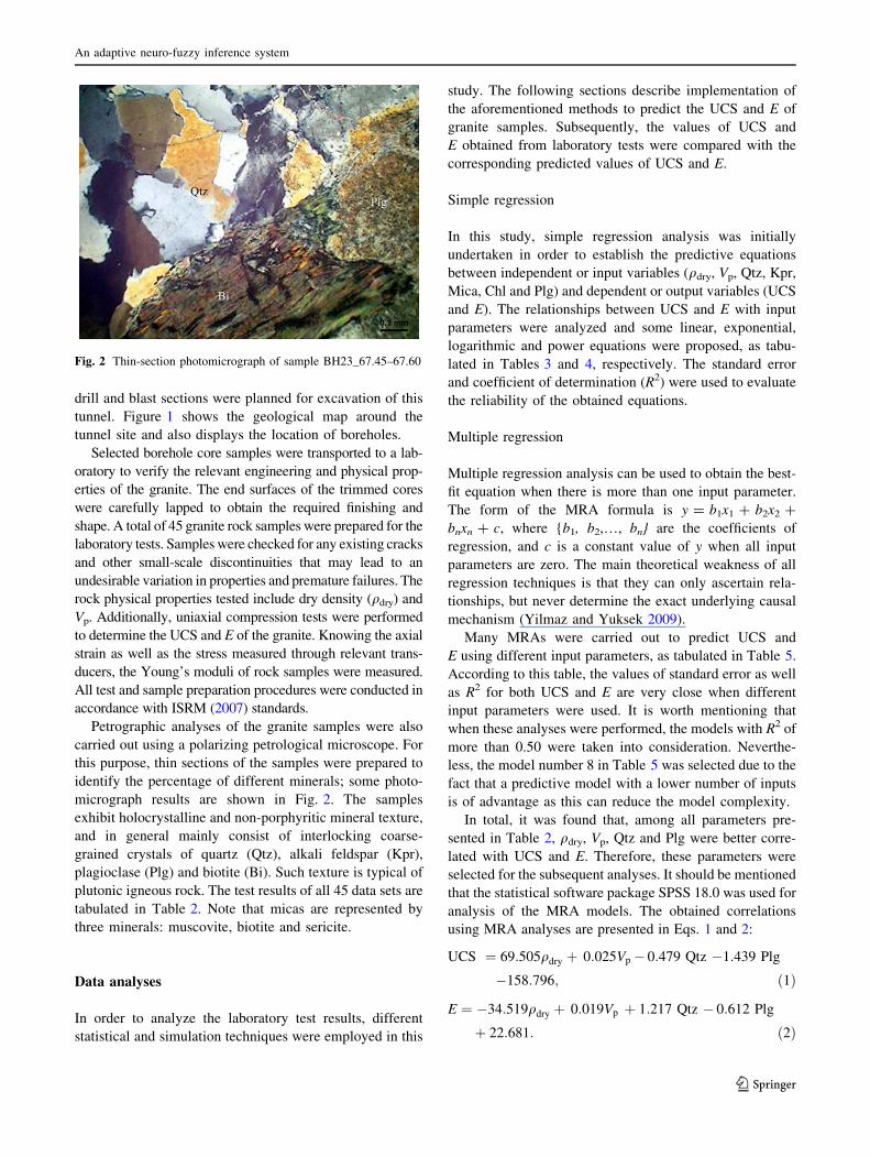
Petrographic analyses of the granite samples were also

carried out using a polarizing petrological microscope. For

this purpose, thin sections of the samples were prepared to

identify the percentage of different minerals; some photo-

micrograph results are shown in Fig. 2. The samples

exhibit holocrystalline and non-porphyritic mineral texture,

and in general mainly consist of interlocking coarse-

grained crystals of quartz (Qtz), alkali feldspar (Kpr),

plagioclase (Plg) and biotite (Bi). Such texture is typical of

plutonic igneous rock. The test results of all 45 data sets are

tabulated in Table 2. Note that micas are represented by

three minerals: muscovite, biotite and sericite.

Data analyses

In order to analyze the laboratory test results, different

statistical and simulation techniques were employed in this

study. The following sections describe implementation of

the aforementioned methods to predict the UCS and E of

granite samples. Subsequently, the values of UCS and

E obtained from laboratory tests were compared with the

corresponding predicted values of UCS and E.

Simple regression

In this study, simple regression analysis was initially

undertaken in order to establish the predictive equations

between independent or input variables (qdry, Vp, Qtz, Kpr,

Mica, Chl and Plg) and dependent or output variables (UCS

and E). The relationships between UCS and E with input

parameters were analyzed and some linear, exponential,

logarithmic and power equations were proposed, as tabu-

lated in Tables 3 and 4, respectively. The standard error

and coefficient of determination (R2) were used to evaluate

the reliability of the obtained equations.

Multiple regression

Multiple regression analysis can be used to obtain the best-

fit equation when there is more than one input parameter.

The form of the MRA formula is y = b1x1 ? b2x2 ?

bnxn ? c, where {b1, b2,…, bn} are the coefficients of

regression, and c is a constant value of y when all input

parameters are zero. The main theoretical weakness of all

regression techniques is that they can only ascertain rela-

tionships, but never determine the exact underlying causal

mechanism (Yilmaz and Yuksek 2009).

Many MRAs were carried out to predict UCS and

E using different input parameters, as tabulated in Table 5.

According to this table, the values of standard error as well

as R2 for both UCS and E are very close when different

input parameters were used. It is worth mentioning that

when these analyses were performed, the models with R2 of

more than 0.50 were taken into consideration. Neverthe-

less, the model number 8 in Table 5 was selected due to the

fact that a predictive model with a lower number of inputs

is of advantage as this can reduce the model complexity.

In total, it was found that, among all parameters pre-

sented in Table 2, qdry, Vp, Qtz and Plg were better corre-

lated with UCS and E. Therefore, these parameters were

selected for the subsequent analyses. It should be mentioned

that the statistical software package SPSS 18.0 was used for

analysis of the MRA models. The obtained correlations

using MRA analyses are presented in Eqs. 1 and 2:

UCS ¼ 69:505qdry þ 0:025Vp� 0:479 Qtz �1:439 Plg

�158:796; ð1Þ

E ¼ �34:519qdry þ 0:019Vp þ 1:217 Qtz � 0:612 Plg

þ 22:681: ð2Þ

Fig. 2 Thin-section photomicrograph of sample BH23_67.45–67.60

An adaptive neuro-fuzzy inference system

123

Table 2 Mineralogical and other properties of the granite samples

Sample

number

Sample

name

Petrographic

name

qdry

(g/cm3)

Vp

(m/s)

Qtz

(%)

Kpr

(%)

Plg

(%)

Chl

(%)

Mica

(%)

UCS

(Mpa)

E

(Gpa)

1 TDH7_35.1–35.4 Microgranite 2.05 3,070 19 15 45 3 18 15 5.7

2 TDH7_38.2–38.4 Microgranite 2.21 3,440 16 14 51 2 15 26 13

3 TDH7_54.6–54.95 Coarse grained granite 2.35 3,660 22 35 28 5 10 39 13.1

4 TDH10_241.0–2411.3 Microgranite 2.72 4,860 32.1 33 22.4 2 10 144 52.7

5 TDH10_278.6–279.0 Microgranite 2.68 5,840 29.7 29 27.3 3 11 161 70.1

6 TDH10_305.7–306.0 Microgranite 2.68 5,830 29.3 25.2 32.5 0 13 176 73.2

7 TDH11_292.6–292.9 Medium grained granite 2.62 5,700 23.5 22.5 36 4 14 60 34.9

8 TDH13_124.1–124.5 Medium to coarse grained granite 2.65 5,370 29.4 28.2 31 0 11 132 50.9

9 TDH13_156.8–157.0 Medium to coarse grained granite 2.64 5,360 30.4 32 26 3 8 54 45.2

10 TDH15_113.7–113.9 Medium to coarse grained granite 2.7 5,260 30.5 35 22 4 8.5 133 61.7

11 TDH16_51.6–51.8 Medium to coarse grained granite 2.58 5,050 32 31 29 0 8 75 46.7

12 TDH17_43.2–43.6 Fine grained granite 2.62 5,420 27.9 31 30.1 0 11 38 30.3

13 TDH17_99.8–100.1 Medium to coarse grained granite 2.62 5,540 30.1 27 34 1 7.9 51 51.8

14 TDH18_52.1–52.4 Coarse grained granite 2.54 4,930 25.5 35 29.5 0 10 71 34.7

15 TDH18_67.3–67.5 Coarse grained granite 2.57 5,320 24 37 34 0 5 78 52.4

16 TDH19_125.0–125.2 Coarse grained granite 2.62 5,370 30.5 33 28.5 0 8 153 66.5

17 TDH19_130.6–131.0 Coarse grained granite 2.62 5,250 28.1 35 20 1 9 148 50.9

18 TDH20_43.5–43.8 Coarse grained granite 2.55 2,700 29.7 32.3 28 1 9 57 18.6

19 TDH20_44.5–44.8 Coarse grained granite 2.64 4,120 37.6 31.4 22 0 9 75 51.4

20 TDH20_48.5–48.8 Coarse grained granite 2.67 4,520 35.1 39.9 15 0 7 75 39.7

21 BH18_55.8–56.1 Bi granite 2.48 4,820 35 30 32 4 6 21.9 13.6

22 BH18_295.6–295.9 Leucogranite 2.72 6,570 30 39 22 4 6 54.7 35.6

23 BH19 _198.7–199.0 Porphyry granite 2.67 7,072 50 45 0 3 8 98 51.9

24 BH20_88.1–88.55 Coarse–grained protomylonite granite 2.6 4,427 35 35 20 3 8 124.5 59.4

25 BH20_93–93.6 Coarse–grained protomylonite granite 2.59 4,765 35 35 20 3 9 113 55

26 BH20 _94.4–94.7 Porphyritic bi granite 2.71 5,842 35 30 33 0 7 21.9 11.3

27 BH21_157.0–157.4 Coarse–grained protomylonite granite 2.53 4,385 35 35 19 0 7 47.3 22.5

28 BH21_158.4–158.8 Coarse–grained protomylonite granite 2.61 6,482 33 34 22 4 1 147.1 73.3

29 BH21_160.1–160.5 Coarse–grained protomylonite granite 2.64 4,450 33 35 19 4 1.5 128.6 60.6

30 BH21_165.0–165.4 Coarse–grained protomylonite granite 2.62 4,560 35 35 18 0 6 98 53.9

31 BH21_165.7–166.0 Bi granite 2.76 6,175 37 28 30 0 5 84.2 46.3

32 BH23_67.45–67.6 Coarse grained granite 2.58 4,707 33 31 29 0 5 85.3 43

33 BH23 _70.4–70.7 Bi granite 2.59 6,610 32 32 33 0 8 136.1 59

34 BH23_70.8–71.0 Coarse grained granite 2.6 4,385 33 31 29 0 8 96 65.7

35 BH24_52.1–52.5 Coarse grained granite 2.65 7,242 40 27 30 0 3 127.9 116.3

36 BH24_74.6–74.8 Coarse–grained protomylonite granite 2.62 5,402 36 32 27 0 3 73 53.6

37 BH24_78.75–78.95 Coarse–grained protomylonite granite 2.62 5,117 37 31 26 0 5 204.9 142.3

38 BH25_150–155 Coarse grained leucoggranite 2.58 5,525 37 31 27 2 9 130.9 130.9

39 BH25_155.5–155.9 Coarse grained leucoggranite 2.66 8,550 39 29 23 0 3 98.9 93.3

40 BH25_164.7–165.0 Bi granite 2.70 6,742 33 30 35 0 2 188.9 96.9

41 BH25_170–175 Coarse grained granite 2.59 5,497 35 33 26 0 9 183.9 90.1

42 BH26_160.7–160.95 Coarse grained granite 2.63 5,095 33 33 29 0 9 195.9 91.9

43 BH26_167.65–167.85 Coarse grained granite 2.65 5,305 33 32 26 0 5 156.8 100.6

44 BH26_172.8–173.0 Coarse grained granite 2.76 7,702 34 28 29 0 5 146.9 74.9

45 BH26_173.55–173.75 Coarse grained granite 2.65 5,370 32 31 29 0 2 85.9 55.1

Qtz quartz, Kpr alkali feldspar, Plg plagioclase, Chl chlorite

D. J. Armaghani et al.

123

Model summaries of MRA for prediction of UCS and

E are illustrated in Table 6.

Artificial neural network

The ANN is an artificial intelligence technique that has

been demonstrated to solve many composite engineering

problems successfully. It is an information-processing

system in which system information is processed by

several interconnected simple elements that are known as

nodes or neurons, positioned in the network layers. The

best ANN has been identified as the multilayer perceptron

(MLP) model, which is composed of three different lay-

ers: input, output and hidden layers (Dreyfus 2005; Jahed

Armaghani et al. 2013). The nodes are linked from one

layer to the next, but this connection is not within the

same layer. After processing the information, the con-

nection links transmit the information between the neu-

rons. A weight is assigned to each link, which is

multiplied into the transmitted signal. The total weighted

input signal of each node is usually transmitted via a

nonlinear activation function.

Performance of an ANN is directly dependent on the

architecture of layers and the number of neurons, which is

the pattern of the connections between the neurons (Haji-

hassani et al. 2014). The BP algorithm is considered the most

popular and effective learning algorithm for multilayered

networks (Tawadrous and Katsabanis 2007). In BP, the

connection weights are adjusted to reduce the errors of

output (Jahed Armaghani et al. 2014). Initially, the network

runs with connection weights that are selected randomly. In

a feed-forward (FF) BP algorithm, the signals flow from the

input layer to the output layer. Finally, a desired output is

computed by the network, and then the difference between

the actual outputs and the desired one is calculated. Network

error is defined as the difference between the real values and

those predicted by the system. The network error in each step

is propagated back, and the individual weights are updated

accordingly. This process is iterated until the error con-

verges to a level that is known by some cost functions, such

as root mean squared error (RMSE) (Simpson 1990; Kosko

Table 3 Results of simple

regression analyses for UCS

prediction

Regression model Predictor Regression function SE R2

Linear qdry UCS = 240.9 9 qdry - 524.61 41.69 R2 = 0.354

Vp UCS = 0.0308 9 E - 61.602 37.82 R2 = 0.468

Plg UCS = -2.4683 9 Plg ? 169.63 48.01 R2 = 0.143

Qtz UCS = 4.3006 9 Qtz - 35.371 45.61 R2 = 0.227

Kpr UCS = 2.3968 9 Kpr ? 27.193 50.21 R2 = 0.063

Mica UCS = -3.563 9 Mica ? 129.63 50.25 R2 = 0.0611

Chl UCS = -6.718 9 Chl ? 110.84 50.63 R2 = 0.0469

Exponential qdry UCS ¼ 0:0111e3:4437�qdry 40.33 R2 = 0.4721

Vp UCS ¼ 12:861e0:0004�Vp 54.42 R2 = 0.416

Plg UCS = 215.95e-0.0339Plg 50.24 R2 = 0.1707

Qtz UCS = 14.346e0.05639Qtz 48.08 R2 = 0.2536

Kpr UCS = 23.548e0.04179Kpr 52.58 R2 = 0.1237

Mica UCS = 140.6e-0.0639Mica 52.82 R2 = 0.124

Chl UCS = 97.913e - 0.094 9 Chl 52.77 R2 = 0.0595

Logarithmic qdry UCS = 568.87ln(qdry) - 441.05 42.26 R2 = 0.3361

Vp UCS = 154.87ln(Vp) – 1,222.6 38.51 R2 = 0.4487

Plg – – –

Qtz UCS = 125.82ln(Qtz) - 331.65 45.62 R2 = 0.2265

Kpr UCS = 69.192ln(Kpr) - 134.81 49.86 R2 = 0.0759

Mica UCS = - 19.95ln(Mica) ? 140.16 50.42 R2 = 0.0551

Chl – – –

Power qdry UCS = 0.0324 9 qdry8.2646 40.79 R2 = 0.4635

Vp UCS = 9E-06 9 Vp1.8797 39.25 R2 = 0.4318

Plg – – –

Qtz UCS = 0.2198 9 Qtz1.7339 47.23 R2 = 0.281

Kpr UCS = 1.2129 9 Kpr1.2465 52.34 R2 = 0.1608

Mica UCS = 157.15 9 Mica-0.312 52.85 R2 = 0.0881

Chl – – –

An adaptive neuro-fuzzy inference system

123

1994). The scenario for the pth pattern in an FF neural net-

work is presented in the following steps:

1. The ith node in the input layer holds a value of xpi for

the pth pattern.

2. Net input to the jth neuron in the hidden layer for

pattern p is:

netpj ¼XN

i

WijOpi; ð3Þ

where Wij is the weight from node i to j. The output

from each unit j is the threshold function, fj, which acts

on the weighted sum. In this MLP model, fj is the

sigmoid function as follows:

f ðnetÞ ¼ 1=ð1þ e�KnetÞ; ð0 \ f ðnetÞ\1Þ; ð4Þ

where k is a positive constant that controls the function

spread.

3. Output of the jth node is defined as:

Opj ¼ fjðnetpjÞ: ð5Þ

4. Net input to the kth neuron of the output layer is:

netk ¼XN

j

WkjXpj; ð6Þ

where Wkj is the weight value between the kth output

layer node and the ith hidden layer.

5. Output of the kth node of the output layer is:

Opk ¼ fkðnetkÞ: ð7Þ

6. Ep is the function error for a pattern, p:

Ep ¼1

2

XN

k

ðtpk � OpkÞ2; ð8Þ

where Opk and tpk are the real and target outputs for

pattern p on neuron k, respectively.

As mentioned previously, qdry, Vp, Qtz and Plg were

selected as model inputs to predict UCS and E. In this

study, all 45 data sets were randomly distributed into two

different data set categories, namely training and testing. In

Table 4 Results of simple

regression analyses for

E prediction

Regression model Predictor Regression function SE R2

Linear qdry E = 122.45 9 qdry - 261.86 26.59 R2 = 0.2579

Vp E = 0.0205 9 E - 52.172 19.91 R2 = 0.5841

Plg E = -1.4884 9 Plg ? 97.395 28.51 R2 = 0.1469

Qtz E = 3.1926 9 Qtz - 45.433 24.84 R2 = 0.3526

Kpr E = 1.6533 9 Kpr ? 4.9675 29.54 R2 = 0.0842

Mica E = -3.4603 9 Mica ? 83.268 28.25 R2 = 0.1628

Chl E = -5.2007 9 Chl ? 63.372 29.62 R2 = 0.0794

Exponential qdry E ¼ 0:0025e3:7843�qdry 26.66 R2 = 0.5015

Vp E ¼ 4:4295e0:0004�Vp 27.39 R2 = 0.5635

Plg E = 122.9e-0.0359Plg 29.41 R2 = 0.1641

Qtz E = 4.8629e0.07129Qtz 25.76 R2 = 0.3567

Kpr E = 10.93e0.04689Kpr 30.69 R2 = 0.1376

Mica E = 95.612e-0.0929Mica 29.67 R2 = 0.2319

Chl E = 55.754e-0.1279Chl 30.86 R2 = 0.0966

Logarithmic qdry E = 291.69ln(qdry) - 221.8 26.75 R2 = 0.2495

Vp E = 103.25ln(Vp) - 826.52 20.41 R2 = 0.563

Plg – – –

Qtz E = 89.529ln(Qtz) - 252 25.39 R2 = 0.3237

Kpr E = 44.836ln(Kpr) - 96.858 29.45 R2 = 0.0899

Mica E = - 18.2ln(Mica) ? 91.288 28.81 R2 = 0.1295

Chl – – –

Power qdry E = 0.0077 9 qdry9.1431 26.58 R2 = 0.499

Vp E = 7E-08 9 Vp2.3748 21.78 R2 = 0.6063

Plg – – –

Qtz E = 0.0278 9 Qtz2.1575 25.25 R2 = 0.3826

Kpr E = 0.3877 9 Kpr1.4027 30.69 R2 = 0.1791

Mica E = 110.14 9 Mica-0.444 30.82 R2 = 0.1569

Chl – – –

D. J. Armaghani et al.

123

this manner, 80 % of the data sets were assigned for

training purposes while the further 20 % was used for

testing of the network performance. In order to obtain

superior performance of the ANN model, it is necessary to

determine the optimal network architecture. According to

Hornik et al. (1989), a network with one hidden layer can

approximate any continuous function. Therefore, one hid-

den layer was utilized in this study. Establishing the

number of neurons in the hidden layer is the most critical

task in the ANN architecture (Sonmez et al. 2006; Sonmez

and Gokceoglu 2008). Different equations have been pro-

posed to determine the number of neurons in hidden layers

by several researchers, as tabulated in Table 7. According

to this table, for the problem at hand, the number of

Table 5 Results of multiple

regression analyses for UCS and

E

Model no. Input Output SE R2

UCS E UCS E

1 qdry, Vp, Qtz UCS, E 36.64 18.54 0.524 0.656

2 qdry, Vp, Kpr UCS, E 36.79 19.44 0.520 0.622

3 qdry, Vp, Plg UCS, E 35.87 18.76 0.544 0.648

4 qdry, Vp, Chl UCS, E 36.72 20.32 0.522 0.587

5 qdry, Vp, Mica UCS, E 36.64 19.88 0.524 0.604

6 qdry, Vp, Qtz, Mica UCS, E 36.39 18.77 0.542 0.656

7 qdry, Vp, Qtz, Kpr UCS, E 37.08 18.53 0.524 0.664

8 qdry, Vp, Qtz, Plg UCS, E 36.27 18.48 0.545 0.667

9 qdry, Vp, Qtz, Chl UCS, E 36.93 18.75 0.528 0.656

10 qdry, Vp, Kpr, Plg UCS, E 35.57 18.98 0.562 0.648

11 qdry, Vp, Kpr, Mica UCS, E 36.84 19.57 0.530 0.626

12 qdry, Vp, Kpr, Chl UCS, E 37.11 19.68 0.523 0.621

13 qdry, Vp, Plg, Mica UCS, E 35.96 18.67 0.552 0.659

14 qdry, Vp, Mica, Chl UCS, E 36.96 20.12 0.527 0.605

15 qdry, Vp, Qtz, Kpr, Plg UCS, E 35.83 18.69 0.567 0.667

16 qdry, Vp, Qtz, Kpr, Chl UCS, E 37.39 18.76 0.529 0.665

17 qdry, Vp, Qtz, Kpr, Mica UCS, E 36.75 18.75 0.545 0.665

18 qdry, Vp, Plg, Mica, Chl UCS, E 36.41 18.85 0.533 0.661

19 qdry, Vp, Qtz, Plg, Mica UCS, E 36.39 18.67 0.553 0.668

20 qdry, Vp, Kpr, Plg, Mica UCS, E 35.99 18.72 0.563 0.666

21 qdry, Vp, Qtz, Kpr, Chl, Mica UCS, E 37.01 18.99 0.548 0.665

22 qdry, Vp, Qtz, Kpr, Mica, Plg UCS, E 36.18 18.91 0.569 0.668

23 qdry, Vp, Qtz, Kpr, Chl, Plg UCS, E 36.24 18.93 0.568 0.667

24 qdry, Vp, Qtz, Mica, Chl, Plg UCS, E 36.85 18.91 0.554 0.669

25 qdry, Vp, Kpr, Mica, Chl, Plg UCS, E 36.46 18.84 0.563 0.670

26 qdry, Vp, Qtz, Kpr, Mica, Chl, Plg UCS, E 36.27 19.11 0.579 0.671

Table 6 Model summaries of the MRA model for prediction of UCS

and E

Independent variable Coefficients SE t value p value

For UCS

Constant -158.796 162.835 -0.975 0.335

qdry 69.505 63.632 1.092 0.281

Vp 0.025 0.006 3.859 0.000

Qtz -0.479 1.5891 -0.302 0.764

Plg -1.439 1.062 -1.354 0.183

For E

Constant 22.681 82.942 0.273 0.786

qdry -34.519 32.412 -1.065 0.293

Vp 0.019 0.003 5.714 0.000

Qtz 1.217 0.809 1.504 0.141

Plg -0.612 0.541 -1.131 0.264

Table 7 The proposed number of neurons for the hidden layer

Heuristic References

B2 9 Ni ? 1 Hecht-Nielsen (1987)

(Ni ? NO)/2 Ripley (1993)

2Ni/3 Wang (1994)ffiffiffiffiffiffiffiffiffiffiffiffiffiffiffiffiffiNi � NO

pMasters (1994)

2Ni Kaastra and Boyd (1996),

Kanellopoulas and Wilkinson (1997)

Ni number of input neurons, NO number of output neurons

An adaptive neuro-fuzzy inference system

123

neurons that might be used in the hidden layer varies

between 2 and 9. In order to determine the optimum

number of neurons in the hidden layer, using the trial-error

method, several networks with one hidden layer were

trained and tested as tabulated in Tables 8 and 9 for the

prediction of UCS and E, respectively. As shown in these

tables, each model was iterated five times. These tables

show the results in terms of R2 and RMSE for the training

and testing data sets. According to the presented results,

model number 3 with four hidden nodes (second iteration)

and model number 2 with three hidden nodes (4th iteration)

indicate higher prediction performances for UCS and E,

respectively, compared to other models. Therefore, these

models, i.e., models 2 and 3, were chosen as the best ANN

models for prediction of UCS and E, respectively. It should

be mentioned that model performance was evaluated based

on both training and testing data sets. It is also worth

mentioning that in construction of ANN models, the

learning rate and momentum coefficient were set to 0.05

and 0.9, respectively.

Adaptive neuro-fuzzy inference system

The ANFIS was developed by Jang (1993). This system is

capable of approximating any actual continuous function at

any accuracy level (Jang et al. 1997). Therefore, a functional

mapping can be modeled by ANFIS that approximates the

prediction process of the internal system parameter. ANFIS

is an artificial intelligence method that integrates the FIS

concept into the ANN and has been extensively utilized in the

field of geotechnical engineering (Grima et al. 2000; Go-

kceoglu et al. 2004; Iphar et al. 2008; Yilmaz and Yuksek

2009; Sezer et al. 2014). Mapping relations between the

input and output parameters through hybrid learning for the

determination of the membership function distribution can

be simulated by ANFIS. A typical ANFIS network archi-

tecture with two input variables (x, y) and one output (f) is

shown in Fig. 3. It is comprised of five layers in the inference

system, and each layer includes several nodes, which are

defined by the node function.

For previous layers, the output neuron is identified as the

input signal in the present layer. After manipulation by the

node function in the present layer, the output will serve as

input signal for the next layer. To describe the procedure of

ANFIS in brief, x and y as inputs and f as output are considered

in the FIS models. Therefore, two fuzzy ‘‘if-then’’ rules can be

constructed as follows (Takagi and Sugeno 1985):

If x is A1 and y is B1 then f 1 ¼ p1xþ q1yþ r1; ðrule 1ÞIf x is A2 and y is B2 then f 2 ¼ p2xþ q2yþ r2; ðrule 2Þ

where A1, A2, B1 and B2 are the membership functions for

inputs x and y; p1, q1, r1, p2, q2 and r2 are the parameters of Ta

ble

8P

erfo

rman

ces

of

trai

ned

AN

Nm

od

els

inp

red

icti

ng

UC

S

Mo

del

no

.

No

des

in hid

den

lay

ers

Net

wo

rkre

sult

Iter

atio

n1

Iter

atio

n2

Iter

atio

n3

Iter

atio

n4

Iter

atio

n5

Tra

inT

est

Tra

inT

est

Tra

inT

est

Tra

inT

est

Tra

inT

est

R2

RM

SE

R2

RM

SE

R2

RM

SE

R2

RM

SE

R2

RM

SE

R2

RM

SE

R2

RM

SE

R2

RM

SE

R2

RM

SE

R2

RM

SE

12

0.8

63

16

.16

60

.88

51

5.4

24

0.8

41

16

.76

50

.90

11

5.7

24

0.8

03

18

.23

60

.86

51

5.9

64

0.7

93

19

.57

60

.79

42

0.4

09

0.8

08

16

.04

30

.89

51

5.0

94

23

0.8

89

15

.65

40

.80

41

6.4

44

0.8

96

15

.13

70

.87

11

6.1

29

0.8

32

16

.89

70

.78

41

7.8

34

0.7

67

18

.16

60

.81

51

5.9

60

0.7

61

18

.52

00

.80

51

5.0

04

34

0.8

77

16

.21

00

.84

91

4.7

80

0.9

12

13

.54

40

.90

61

2.5

73

0.8

19

16

.19

00

.85

51

6.0

03

0.8

22

16

.81

00

.86

51

6.4

50

0.8

90

14

.55

50

.80

61

5.8

74

45

0.7

81

21

.12

00

.84

61

5.7

80

0.7

53

19

.00

60

.67

52

1.4

23

0.9

01

14

.11

00

.86

61

5.4

22

0.8

18

17

.22

60

.90

91

4.1

04

0.7

33

20

.09

20

.81

11

6.9

84

56

0.8

39

15

.87

60

.71

51

9.4

94

0.8

88

16

.16

60

.88

51

5.9

84

0.8

14

16

.77

70

.82

91

5.6

54

0.9

07

15

.09

60

.84

41

6.2

20

0.8

55

16

.44

60

.81

11

7.4

64

67

0.8

48

16

.78

10

.80

11

7.4

10

0.7

88

19

.18

60

.83

11

5.8

89

0.7

18

16

.16

60

.81

01

5.7

36

0.8

87

15

.22

50

.86

81

5.4

77

0.8

49

16

.10

60

.67

22

0.5

58

78

0.9

02

14

.64

10

.87

71

5.8

94

0.7

13

19

.10

90

.63

52

1.7

02

0.8

95

15

.14

40

.83

01

5.8

86

0.6

80

21

.77

60

.89

51

4.9

80

0.8

80

15

.46

30

.88

21

5.4

53

89

0.8

99

15

.13

60

.86

91

5.7

01

0.8

44

16

.63

50

.86

71

5.5

51

0.8

92

15

.34

40

.86

01

5.7

89

0.7

42

20

.96

60

.76

52

1.6

64

0.7

60

19

.74

70

.68

82

1.4

55

D. J. Armaghani et al.

123

the output function. In the following, the five-layer ANFIS

including two fuzzy rules, x and y (inputs), and one output

(f) is presented (Jang 1993; Jang et al. 1997):

Layer 1 All nodes i in this layer are adaptive nodes:

O1;i ¼ lAiðxÞ; ð9Þ

O1;i ¼ lBiðyÞ; ð10Þ

for i = 1, 2 where x and y are considered as input neurons,

and A and B are the linguistic labels. Also, lAi(x) and

lBi(y) are the membership functions.

Layer 2 The nodes are labeled P and identified by a

circle. The output neuron is created by all the incoming

signals:

O2;i ¼ xi ¼ lAiðxÞ lBiðyÞ with i ¼ 1; 2: ð11Þ

The output neuron xi presents the firing strength of a rule.

Layer 3 Every node in this layer is a fixed node to be

marked by a circle and labeled as N. The output is com-

puted by the ratio of the ith rule’s firing strength over the

sum of all rules’ firing strength:

O3;i ¼ -i ¼ xi=ðx1 þ x2Þ with i ¼ 1; 2: ð12Þ

Layer 4 In this layer, every node is an adaptive node

with the node function as follows:

O4;i ¼ -ifi ¼ -iðpixþ qiyþ riÞ; ð13Þ

where parameters pi, qi and ri are named the consequent

parameters. A normalized firing strength is named -i.

Layer 5 In this layer (final step), the output amount is

created by the sum of all incoming signals:

O5;i ¼X

i

-ifi ¼X

i

-ifi=X

i

-i; i ¼ 1; 2: ð14Þ

BP gradient descent is the basic learning rule of the

ANFIS, which computes error signals recursively from the

output layer backward to the input nodes. Based on the

architecture in Fig. 3b, the output (f) can be stated as a

linear combination of the consequent parameters. To learn

the fuzzy model employing differentiable functions, the

ANFIS utilizes a hybrid-learning rule as it is easy to use.

The classical BP technique is used by the ANFIS to learn

the parameters of membership functions. Also, the con-

ventional least-squares predictor is applied by the ANFIS

to learn the parameter of the first-order polynomial of the

Takagi-Sugeno-Kang fuzzy model (Jang et al. 1997).

In the procedure of the ANFIS, there are two different

passes of hybrid learning (forward and backward). In the

forward pass, functional signals go forward until the fourth

layer, and the consequent parameters are investigated by

the least-squares estimate. Similar to the ANN procedure,

the system errors are propagated back and the premise

parameters are updated using the gradient descent in the

backward pass. The final output can be defined as follows:Ta

ble

9P

erfo

rman

ces

of

trai

ned

AN

Nm

od

els

inp

red

icti

ng

E

Mo

del

no

.

No

des

in hid

den

lay

ers

Net

wo

rkre

sult

Iter

atio

n1

Iter

atio

n2

Iter

atio

n3

Iter

atio

n4

Iter

atio

n5

Tra

inT

est

Tra

inT

est

Tra

inT

est

Tra

inT

est

Tra

inT

est

R2

RM

SE

R2

RM

SE

R2

RM

SE

R2

RM

SE

R2

RM

SE

R2

RM

SE

R2

RM

SE

R2

RM

SE

R2

RM

SE

R2

RM

SE

12

0.8

98

13

.56

60

.92

09

.89

70

.87

51

5.1

05

0.9

03

11

.16

70

.84

31

6.4

31

0.9

08

11

.38

40

.80

91

7.6

18

0.8

10

16

.36

80

.82

41

4.4

39

0.9

13

10

.58

5

23

0.9

25

10

.10

40

.83

61

4.8

16

0.9

20

9.6

38

0.9

15

9.5

32

0.8

74

15

.22

40

.82

31

5.0

68

0.9

27

8.7

12

0.9

18

9.1

87

0.8

96

13

.66

80

.89

91

2.5

04

34

0.9

12

10

.60

50

.88

31

3.3

17

0.9

23

9.2

03

0.9

09

11

.32

80

.86

01

4.5

87

0.8

98

14

.41

90

.83

81

5.1

29

0.8

82

14

.80

50

.81

51

5.1

08

0.8

22

14

.28

7

45

0.8

12

15

.02

90

.88

01

4.2

18

0.7

83

16

.12

40

.70

91

9.3

02

0.9

16

12

.71

30

.90

91

0.8

95

0.8

34

15

.50

30

.91

71

2.6

94

0.7

48

17

.08

30

.82

71

5.2

86

56

0.8

73

14

.30

40

.74

41

7.5

64

0.9

24

10

.16

60

.91

01

0.4

02

0.8

55

15

.11

60

.87

01

4.1

04

0.9

25

8.8

86

0.8

61

14

.59

80

.87

21

4.8

01

0.8

27

15

.71

8

67

0.8

82

15

.12

00

.83

31

5.6

86

0.8

20

15

.28

70

.87

31

4.3

16

0.7

54

14

.56

60

.85

11

4.1

78

0.9

05

10

.70

30

.88

51

3.9

29

0.8

66

14

.49

50

.68

51

8.5

02

78

0.9

12

11

.19

20

.91

41

1.3

20

0.7

42

17

.21

70

.66

71

9.5

54

0.9

11

13

.64

50

.87

21

4.3

13

0.6

94

18

.59

80

.91

31

3.4

82

0.9

01

13

.91

70

.90

01

3.9

08

89

0.9

15

9.6

38

0.9

04

11

.14

70

.87

81

4.9

88

0.9

10

11

.01

10

.87

11

3.8

25

0.9

03

11

.22

60

.75

71

7.8

69

0.7

80

19

.49

80

.77

51

7.7

72

0.7

02

19

.31

0

An adaptive neuro-fuzzy inference system

123

f ¼ x1

x1 þ x2

f1 þx1

x1 þ x2

f2

¼ -1ðp1xþ q1yþ r1Þ þ -2ðp2xþ q2yþ r2Þ¼ ð-1xÞp1 þ ð-1yÞq1 þ ð-1Þr1 þ ð-2xÞp2 þ ð-2yÞq2

þ ð-2Þr2; ð15Þ

in which p1, q1, r1, p2, q2 and r2 are consequent parameters.

The advantage of using the ANFIS model is that the con-

sequent parameters and optimal premise parameters can be

efficiently obtained in the learning process.

In this study, a hybrid intelligent system (ANFIS) for

predicting UCS and E of granite was also applied. Similar

to the ANN analyses part, all data sets were distributed

randomly to training (80 %) and testing (20 %) data sets.

In fact the idea behind using the testing data set is to verify

the generalization capability of the proposed neural net-

work model. The use of the random sampling procedure

has been reported in several studies (Alvarez and Babuska

1999; Singh et al. 2001; Rabbani et al. 2012; Tonnizam

Mohamad et al. 2014). In order to determine the number of

fuzzy rules, using a trial-error method, many models of the

fuzzy rule combinations (e.g., 2 and 3) were employed for

the UCS and E data sets separately. Eventually, it was

found that input parameters with three fuzzy rules outper-

form the other ANFIS models for both UCS and E predic-

tion. For the ANFIS modeling part, to select the optimum

number of fuzzy rules, a parametric study was conducted.

It was found that a number of 81 fuzzy rules

(3 9 3 9 3 9 3) shows the best performance in predicting

UCS and E. However, Table 10 shows parameter types and

their values used in the ANFIS model. In the next step of

the modeling, ANFIS models were constructed to predict

UCS and E. Prediction performance of these two outputs

are presented in Table 11. As shown in these tables, each

model was repeated five times using different training and

testing data sets. Based on the tabulated results in this table,

considering the results of both the training and testing data

sets, model number 3 for UCS prediction and model

number 4 for E prediction indicate higher prediction per-

formances among all five models. Therefore, model num-

ber 3 and model number 4 were selected for prediction of

UCS and E respectively. In this study, all ANFIS models

Fig. 3 a First order Sugeno

fuzzy reasoning; b equivalent

ANFIS architecture (following

Jang et al. 1997)

D. J. Armaghani et al.

123

were trained by utilizing 100 epochs. The assigned mem-

bership functions with categories of low, medium and high

for the best models of UCS and E are shown in Figs. 4, 5, 6

and 7. It is worth mentioning that these membership

functions were assigned after the ANFIS training stage.

Moreover, a linear type of membership function was used

for the output (UCS and E). In order to estimate the

membership functions parameters, a hybrid optimization

method was utilized. It should be noted that all ANN and

ANFIS models used to predict UCS and E were trained

with the help of MATLAB version 7.14.0.739. Addition-

ally, SPSS 18.0 was utilized for RMSE and statistical

calculations.

Results and discussion

In this study an attempt has been made to show the capa-

bility of the MRA, ANN and ANFIS models to predict the

UCS and E of granite. The models of ANFIS, ANN and

MRA, for the prediction of UCS and E, were constructed

using four inputs (qdry, Vp, Qtz and Plg) and two outputs.

The graph of predicted UCS and E using the MRA tech-

nique against the measured UCS and E for all 45 samples is

displayed in Fig. 8. As indicated in this figure, the rela-

tively low R2 values, equal to 0.545 and 0.667, reveal the

low reliability of the MRA technique for prediction of UCS

and E ,respectively. Figures 9 and 10 show the predicted

UCS and E by employing an ANN model plotted against

the measured UCS and E values for the training and testing

data sets, respectively. The R2 values of 0.912 and 0.906

for the training and testing of UCS prediction and also

Table 10 Different parameters used in ANFIS model

ANFIS parameter Value

Input membership function Gaussianmf

Output membership function Linear

Number of nodes 193

Number of linear parameters 405

Number of nonlinear parameters 24

Total number of parameters 429

Number of training data pairs 36

Number of testing data pairs 9

Number of fuzzy rules 81

Table 11 Performances of the

five ANFIS models in

predicting UCS and E

ANFIS model UCS E

Train Test Train Test

R2 RMSE R2 RMSE R2 RMSE R2 RMSE

1 0.965 7.881 0.983 6.560 0.977 3.919 0.973 4.873

2 0.979 7.021 0.972 6.932 0.969 4.091 0.961 4.322

3 0.985 6.373 0.994 5.590 0.988 3.552 0.971 4.677

4 0.981 6.702 0.994 5.772 0.987 3.350 0.995 4.053

5 0.954 7.844 0.968 6.981 0.972 4.230 0.978 4.619

Fig. 4 Assigned membership

functions for the qdry input

parameter

An adaptive neuro-fuzzy inference system

123

0.927 and 0.918 for training and testing of the E prediction

show that the ANN approach is able to predict UCS and

E with relatively suitable accuracy. Furthermore, in the

prediction of UCS and E using the ANFIS model, R2 values

of 0.985 and 0.994 for the training and testing of UCS and

0.987 and 0.995 for the training and testing of E suggest the

Fig. 5 Assigned membership

functions for the Vp input

parameter

Fig. 6 Assigned membership

functions for the Qtz input

parameter

Fig. 7 Assigned membership

functions for the Plg input

parameter

D. J. Armaghani et al.

123

superiority of this model in predicting the UCS and E of

granite (see Figs. 11, 12).

In this study, the RMSE and amount of value account

for (VAF) were computed to control the capacity perfor-

mance of the predictive models developed, as applied by

Alvarez and Babuska (1999) and Gokceoglu (2002):

RMSE ¼

ffiffiffiffiffiffiffiffiffiffiffiffiffiffiffiffiffiffiffiffiffiffiffiffiffiffiffiffiffi1

N

XN

i¼1

ðy� y0 Þ2

vuut ; ð16Þ

VAF ¼ 1� varðy� y0 Þ

varðyÞ

� �� 100; ð17Þ

Fig. 8 R2 of measured and predicted values of UCS and E using the MRA model

Fig. 9 R2 values of the measured and predicted UCS for training and testing data sets using the ANN model

Fig. 10 R2 values of the measured and predicted E for the training and testing data sets using the ANN model

An adaptive neuro-fuzzy inference system

123

where y and y0 are the obtained and estimated values,

respectively, and N is the total number of data. The model

is excellent if the RMSE is zero and VAF is 100. Perfor-

mance indices obtained by predictive models for all 45 data

sets are shown in Table 12. As tabulated in this table, the

ANFIS predictive model can provide higher performance

in the prediction of UCS and E in comparison to other

predictive models. In order to demonstrate a better com-

parison, the RMSE and VAF values for predictive models

are displayed in Fig. 13. According to this figure, the

RMSE and VAF values reveal that the performance

capacity of the ANFIS predictive model is higher than that

of both the MRA and ANN predictive models.

The results demonstrate that all aforementioned models

are applicable when predicting the UCS and E of granite.

However, these approaches should be used according to the

situation. The ANFIS predictive model may be used when

a high degree of accuracy is required. Moreover, the MRA

predictive model can be used in conditions where a simple

estimation of UCS and E is desired.

Conclusion

A total of 45 granite rock samples were collected during

site investigation of the Pahang-Selangor raw water trans-

fer tunnel to predict their UCS and E values. Subsequently,

MRA, ANN and ANFIS predictive models were applied to

predict UCS and E using four inputs: qdry, ultrasonic

velocity, Qtz content and Plg. Prediction results showed

that the ANFIS predictive model can predict UCS and

Fig. 11 R2 values of the measured and predicted UCS for the training and testing data sets using the ANFIS model

Fig. 12 R2 values of the measured and predicted E for the training and testing data sets using the ANFIS model

Table 12 Performance indices of the predictive models for all 45

data sets

Predictive

model

UCS E

R2 RMSE VAF

(%)

R2 RMSE VAF

(%)

MRA 0.545 34.197 54.505 0.667 17.418 66.682

ANN 0.911 13.355 91.098 0.919 8.809 91.496

ANFIS 0.985 6.224 98.455 0.990 3.503 98.968

D. J. Armaghani et al.

123

E much better than the ANN and MRA predictive models.

The R2 values (for all data sets) equal to 0.985 and 0.990

for UCS and E, respectively, express the high reliability of

the ANFIS predictive model, while these values were 0.911

and 0.919 for the ANN model and 0.545 and 0.667 for the

MRA model. Nevertheless, these predictive models can be

applied to predict UCS and E depending on the situation. In

terms of performance, it was also shown that using ANFIS

constitutes a feasible approach to minimizing uncertainties

when designing rock engineering projects. The ANFIS

displays several benefits as it combines the advantages of

ANN and FIS techniques to demonstrate a high prediction

capacity in complex, nonlinear and multivariable engi-

neering problems.

Acknowledgments The authors would like to extend their sincere

gratitude to the Pahang-Selangor Raw Water Transfer Project team,

especially to Ir. Dr. Zulkeflee Nordin, Ir. Arshad and contractor and

consultant groups for facilitating this study. The authors would also

like to express their appreciation to Universiti Teknologi Malaysia for

support and making this study possible. Also, the authors are grateful

to the reviewers for their constructive comments.

References

Alvarez GM, Babuska R (1999) Fuzzy model for the prediction of

unconfined compressive strength of rock samples. Int J Rock

Mech Min Sci 36:339–349

Asadi M, Hossein Bagheripour M, Eftekhari M (2013) Development

of optimal fuzzy models for predicting the strength of intact

rocks. Comput Geosci 54:107–112

Atici U (2011) Prediction of the strength of mineral admixture

concrete using multivariable regression analysis and an artificial

neural network. Expert Syst Appl 38:9609–9618

Basu A, Aydin A (2006) Predicting uniaxial compressive strength by

point load test: significance of cone penetration. Rock Mech

Rock Eng 39:483–490

Beiki M, Majdi A, Givshad AD (2013) Application of genetic

programming to predict the uniaxial compressive strength and

elastic modulus of carbonate rocks. Int J Rock Mech Min Sci

63:159–169

Ceryan N, Okkan U, Kesimal A (2012) Prediction of unconfined

compressive strength of carbonate rocks using artificial neural

networks. Environ Earth Sci 68(3):807–819

Cevik A, Sezer EA, Cabalar AF, Gokceoglu C (2011) Modeling of the

uniaxial compressive strength of some clay-bearing rocks using

neural network. Appl Soft Comput 11(2):2587–2594

Cobanglu I, Celik S (2008) Estimation of uniaxial compressive

strength from point load strength, Schmidt hardness and P-wave

velocity. Bull Eng Geol Environ 67:491–498

Dehghan S, Sattari GH, Chehreh CS, Aliabadi MA (2010) Prediction

of unconfined compressive strength and modulus of elasticity for

Travertine samples using regression and artificial neural net-

works. Min Sci Technol 20:0041–0046

Dreyfus G (2005) Neural networks: methodology and application.

Springer, Berlin

Garret JH (1994) Where and why artificial neural networks are

applicable in civil engineering. J Comput Civil Eng 8:129–130

Gokceoglu C (2002) A fuzzy triangular chart to predict the uniaxial

compressive strength of the Ankara agglomerates from their

petrographic composition. Eng Geol 66(1):39–51

Gokceoglu C, Zorlu K (2004) A fuzzy model to predict the

unconfined compressive strength and modulus of elasticity of a

problematic rock. Eng Appl Artif Intell 17:61–72

Gokceoglu C, Yesilnacar E, Sonmez H, Kayabasi A (2004) Aneu-

rofuzzy model for modulus of deformation of jointed rock

masses. Comput Geotech 31(5):375–383

Grima MA, Bruines PA, Verhoef PNW (2000) Modeling tunnel

boring machine performance by neuro-fuzzy methods. Tunn

Undergr Space Technol 15(3):260–269

Hajihassani M, Jahed Armaghani D, Sohaei H, Tonnizam Mohamad

E, Marto A (2014) Prediction of airblast-overpressure induced

by blasting using a hybrid artificial neural network and particle

swarm optimization. Appl Acoust 80:57–67

Hecht-Nielsen R (1987) Kolmogorov’s mapping neural network

existence theorem. In: Proceedings of the first IEEE international

conference on neural networks, San Diego CA, USA, pp 11–14

Hornik K, Stinchcombe M, White H (1989) Multilayer feedforward

networks are universal approximators. Neural Netw 2:359–366

Iphar M, Yavuz M, Ak H (2008) Prediction of ground vibrations

resulting from the blasting operations in an open-pit mine by

adaptive neuro-fuzzy inference system. Environ Geol 56:97–107

ISRM (2007) The complete ISRM suggested methods for rock

characterization, testing and monitoring: 1974–2006. In: Ulusay

R, Hudson JA (eds) Suggested methods prepared by the

commission on testing methods, International Society for Rock

Mechanics

Fig. 13 Comparison of the RMSE and VAF values for MRA, ANN and ANFIS predictive models

An adaptive neuro-fuzzy inference system

123

Jahed Armaghani D, Hajihassani M, Yazdani Bejarbaneh B, Marto A,

Tonnizam Mohamad E (2014) Indirect measure of shale shear

strength parameters by means of rock index tests through an

optimized artificial neural network. Measurement 55:487–498

JahedArmaghani D, Hajihassani M, Mohamad ET, Marto A, Noorani

SA (2013) Blasting-induced flyrock and ground vibration

prediction through an expert artificial neural network based on

particle swarm optimization. Arab J Geosci. doi:10.1007/

s12517-013-1174-0

Jang RJS (1993) Anfis: adaptive-network-based fuzzy inference

system. IEEE Trans Syst Man Cybern 23:665–685

Jang RJS, Sun CT, Mizutani E (1997) Neuro-fuzzy and soft

computing. Prentice-Hall, Upper Saddle River, p 614

Kaastra I, Boyd M (1996) Designing a neural network for forecasting

financial and economic time series. Neurocomputing 10:215–

236

Kahraman S (2001) Evaluation of simple methods for assessing the

uniaxial compressive strength of rock. Int J Rock Mech Min Sci

38:981–994

Kahraman S (2014) The determination of uniaxial compressive

strength from point load strength for pyroclastic rocks. Eng Geol

170:33–42

Kahraman S, Fener M, Kozman E (2012) Predicting the compressive

and tensile strength of rocks from indentation hardness index. J S

Afr Inst Min Metall 112(5):331–339

Kanellopoulas I, Wilkinson GG (1997) Strategies and best practice

for neural network image classification. Int J Remote Sens

18:711–725

Karaman K, Kesimal A (2014) A comparative study of Schmidt

hammer test methods for estimating the uniaxial compressive

strength of rocks. Bull Eng Geol Environ. doi:10.1007/s10064-

014-0617-5

Kosko B (1994) Neural networks and fuzzy systems: a dynamical

systems approach to machine intelligence. Prentice Hall, New

Delhi

Majdi A, Beiki M (2010) Evolving neural network using a genetic

algorithm for predicting the deformation modulus of rock

masses. Int J Rock Mech Min Sci 47(2):246–253

Marto A, Hajihassani M, Jahed Armaghani D, Tonnizam Mohamad E,

Makhtar AM (2014) A novel approach for blast-induced flyrock

prediction based on imperialist competitive algorithm and

artificial neural network. Sci World J. Article ID 643715

Masters T (1994) Practical neural network recipes in C??. Academic

Press, Boston

Meulenkamp F, Grima MA (1999) Application of neural networks for

the prediction of the unconfined compressive strength (UCS)

from Equotip hardness. Int J Rock Mech Min Sci 36(1):29–39

Mishra DA, Basu A (2013) Estimation of uniaxial compressive

strength of rock materials by index tests using regression

analysis and fuzzy inference system. Eng Geol 160:54–68

Momeni E, Nazir R, JahedArmaghani D, Maizir H (2014a) Prediction

of pile bearing capacity using a hybrid genetic algorithm-based

ANN. Measurement 57:122–131

Momeni E, Jahed Armaghani D, Hajihassani M, Mohd Amin MF

(2014b) Prediction of uniaxial compressive strength of rock

samples using hybrid particle swarm optimization-based artifi-

cial neural networks. Measurement .doi:10.1016/j.measurement.

2014.09.075

Monjezi M, Khoshalan HA, Razifard M (2012) A neuro-genetic

network for predicting uniaxial compressive strength of rocks.

Geotech Geol Eng 30(4):1053–1062

Moradian ZA, Ghazvinian AH, Ahmadi M, Behnia M (2010)

Predicting slake durability index of soft sandstone using indirect

tests. Int J Rock Mech Min Sci 47(4):666–671

Nazir R, Momeni E, Jahed Armaghani D, Mohd Amin MF (2013a)

Correlation between unconfined compressive strength and

indirect tensile strength of limestone rock samples. Electr J

Geotech Eng 18:1737–1746

Nazir R, Momeni E, JahedArmaghani D, Mohd Amin MF (2013b)

Prediction of unconfined compressive strength of limestone rock

samples using L-type Schmidt hammer. Electr J Geotech Eng

18:1767–1775

O’Rourke JE (1989) Rock index properties for geoengineering in

underground development. Miner Eng 106–110

Rabbani E, Sharif F, KoolivandSalooki M, Moradzadeh A (2012)

Application of neural network technique for prediction of

uniaxial compressive strength using reservoir formation proper-

ties. Int J Rock Mech Min Sci 56:100–111

Rezaei M, Majdi A, Monjezi M (2012) An intelligent approach to

predict unconfined compressive strength of rock surrounding

access tunnels in longwall coal mining. Neural Comput Appl

24(1):233–241

Ripley BD (1993) Statistical aspects of neural networks. In: Barndoff-

Neilsen OE, Jensen JL, Kendall WS (eds) Networks and chaos-

statistical and probabilistic aspects. Chapman & Hall, London,

pp 40–123

Sezer EA, Nefeslioglu HA, Gokceoglu C (2014) An assessment on

producing synthetic samples by fuzzy C-means for limited

number of data in prediction models. Appl Soft Comput

24:126–134

Simpson PK (1990) Artificial neural system: foundation, paradigms,

applications and implementations. Pergamon, New York

Singh RN, Hassani FP, Elkington PAS (1983) The application of

strength and deformation index testing to the stability assessment

of coal measures excavations. In: Proceeding of 24th US

symposium on rock mechanism, Texas A and M Univ. AEG,

Balkema, Rotterdam, pp 599–609

Singh VK, Singh D, Singh TN (2001) Prediction of strength

properties of some schistose rocks from petrographic properties

using artificial neural networks. Int J Rock Mech Min Sci

38(2):269–284

Singh R, Kainthola A, Singh TN (2012) Estimation of elastic constant of

rocks using an ANFIS approach. Appl Soft Comput 12(1):40–45

Sonmez H, Gokceoglu C (2008) Discussion on the paper by H. Gullu

and E. Ercelebi, ‘‘A neural network approach for attenuation

relationships: an application using strong ground motion data

from Turkey. Eng Geol 97:91–93

Sonmez H, Tuncay E, Gokceoglu C (2004) Models to predict the

uniaxial compressive strength and the modulus of elasticity for

Ankara Agglomerate. Int J Rock Mech Min Sci 41(5):717–729

Sonmez H, Gokceoglu C, Nefeslioglu HA, Kayabasi A (2006)

Estimation of rock modulus: for intact rocks with an artificial

neural network and for rock masses with a new empirical

equation. Int J Rock Mech Min Sci 43:224–235

Sulukcu S, Ulusay R (2001) Evaluation of the block punch index test

with particular reference to the size effect, failure mechanism

and its effectiveness in predicting rock strength. Int J Rock Mech

Min Sci 38:1091–1111

Takagi T, Sugeno M (1985) Fuzzy identification of systems and itsapplications to modeling and control. IEEE Trans Syst Man

Cybern 15:116–132

Tandon RS, Gupta V (2014) Estimation of strength characteristics of

different Himalayan rocks from Schmidt hammer rebound, point

load index, and compressional wave velocity. Bull Eng Geol

Environ. doi:10.1007/s10064-014-0629-1

Tawadrous AS, Katsabanis PD (2007) Prediction of surface crown

pillar stability using artificial neural networks. Int J Numer Anal

Method 31(7):917–931

Tonnizam Mohamad E, Jahed Armaghani D, Momeni E, Alavi

Nezhad Khalil Abad SV (2014) Prediction of the unconfined

compressive strength of soft rocks: a PSO-based ANN approach.

Bull Eng Geol Environ. doi:10.1007/s10064-014-0638-0

D. J. Armaghani et al.

123

Wang C (1994) A theory of generalization in learning machines with

neural application. PhD thesis, The University of Pennsylvania,

USA

Yagiz S (2011) Correlation between slake durability and rock

properties for some carbonate rocks. Bull Eng Geol Environ

70(3):377–383

Yagiz S, Sezer EA, Gokceoglu C (2012) Artificial neural networks

and nonlinear regression techniques to assess the influence of

slake durability cycles on the prediction of uniaxial compressive

strength and modulus of elasticity for carbonate rocks. Int J

Numer Anal Method 36(14):1636–1650

Yasar E, Erdogan Y (2004) Estimation of rock physiomechanical

properties using hardness methods. Eng Geol 71:281–288

Yesiloglu-Gultekin N, Gokceoglu C, Sezer EA (2013) Prediction of

uniaxial compressive strength of granitic rocks by various

nonlinear tools and comparison of their performances. Int J Rock

Mech Min Sci 62:113–122

Yilmaz I, Sendir H (2002) Correlation of Schmidt hardness with

unconfined compressive strength and Young’s modulus in

gypsum from Sivas (Turkey). Eng Geol 66(3):211–219

Yilmaz I, Yuksek G (2009) Prediction of the strength and elasticity

modulus of gypsum using multiple regression, ANN, and ANFIS

models. Int J Rock Mech Min Sci 46(4):803–810

Zorlu K, Gokceoglu C, Ocakoglu F, Nefeslioglu HA, Acikalin S

(2008) Prediction of uniaxial compressive strength of sandstones

using petrography-based models. Eng Geol 96(3):141–158

An adaptive neuro-fuzzy inference system

123