PREDICTION OF ELASTIC MODULUS FROM COMPESSIVE MODULUS OF LIME STABILIZED LATERITIC SOIL FOR...
24
www.ijecs.in International Journal Of Engineering And Computer Science ISSN:2319-7242 Volume 3 Issue 4 April, 2014 Page No. 5471-5494 D.B.Eme 1 IJECS Volume 3 Issue 4 April, 2014 Page No.5471-5494 Page 5471 PREDICTION OF ELASTIC MODULUS FROM COMPESSIVE MODULUS OF LIME STABILIZED LATERITIC SOIL FOR MECHANISTIC DESIGN USING THE SPLIT CYLINDER 1 D.B.Eme, 2 J.C.Agunwamba 1 Department of Civil Engineering, University of Port Harcourt Nigeria 2 Department of Civil Engineering, University of Nigeria Nsukka ABSTRACT In recent years there has been a change in philosophy in flexible pavement design from the more empirical approach to the mechanistic approach based on the elastic theory. The mechanistic approach is in the form of layered elastic theory which is being used by many agencies. Elastic theory based design methods require as input, the elastic properties of these pavement material for an effective design. In this study laterites were gotten from seven (7) local government areas in Rivers state. The laterites were classified using the AASHTO classification system, the properties obtained from the laterites indicates that it is an A -5 soil which is a silty-clay material. The material was mixed with different lime contents of 0,2,4,6,and 8% and compacted at the energy of Standard Proctor in 100mm diameter by 80mm long split cylindrical moulds, the compacted specimens were moist - cured and tested after 7, 14 ,21 and 28days. The CBR machine was used to load the specimen to failure through static load application. The failure loads as well as the horizontal and vertical strains were measured and used to predict Elastic modulus from compressive modulus using the SPSS programme, the result show that the Elastic and Compressive modulus increases with an increase in lime content up to 8% lime content, also the predicted values were close to the measured values with an average R 2 value of 92%, indicating that the predicted Elastic modulus can be used for mechanistic design of flexible pavement. KEYWORDS: Prediction, Elastic Modulus, Compressive Modulus, Lateritic Soil, Mechanistic Design, Split Cylinder. 1. INTRODUCTION In recent years there has been a change in philosophy in flexible pavement design from the more empirical approach to the mechanistic approach based on the elastic theory [7], [9] and [8]. Proposed by [11], this mechanistic approach in the form layered elastic theory is being used by increasing numbers of agencies. Elastic theory based design methods require as input the elastic properties of these pavement materials for an effective design. In contemporary flexible pavement design ,methods based on elastic theory requires that the elastic properties of the pavement material be known [5] concluded from their work that among the common methods of measurement of elastic properties which are (youngs, shear, bulk, complex, dynamic, double punch, resilient, and shell nomograph moduli) the resilient modulus is more appropriate for use in multilayer elastic theories. Pavement materials include Portland Cement Concrete; Asphalt Concrete Cement bound materials, compacted soils, rocks and sub-grades. They are materials that terminate by fracture at or slightly beyond the yield stress generally referred to as brittle materials. They are isotropic (ie displays the same properties in all directions) and are assumed to be linearly elastic up to a certain stress level (referred to as the elastic limit). Therefore knowledge of the elastic properties of pavement is very essential in elastic theory for the mechanistic design of flexible and rigid pavements, including overlays, in this design method the
Transcript of PREDICTION OF ELASTIC MODULUS FROM COMPESSIVE MODULUS OF LIME STABILIZED LATERITIC SOIL FOR...

www.ijecs.in International Journal Of Engineering And Computer Science ISSN:2319-7242 Volume 3 Issue 4 April, 2014 Page No. 5471-5494
D.B.Eme1IJECS Volume 3 Issue 4 April, 2014 Page No.5471-5494 Page 5471
PREDICTION OF ELASTIC MODULUS FROM COMPESSIVE MODULUS OF
LIME STABILIZED LATERITIC SOIL FOR MECHANISTIC DESIGN USING
THE SPLIT CYLINDER
1D.B.Eme,
2 J.C.Agunwamba
1Department of Civil Engineering, University of Port Harcourt Nigeria
2Department of Civil Engineering, University of Nigeria Nsukka
ABSTRACT
In recent years there has been a change in philosophy in flexible pavement design from the more empirical approach to the
mechanistic approach based on the elastic theory. The mechanistic approach is in the form of layered elastic theory which is being
used by many agencies. Elastic theory based design methods require as input, the elastic properties of these pavement material for
an effective design. In this study laterites were gotten from seven (7) local government areas in Rivers state. The laterites were
classified using the AASHTO classification system, the properties obtained from the lateri tes indicates that it is an A -5 soil which
is a silty-clay material. The material was mixed with different lime contents of 0,2,4,6,and 8% and compacted at the energy of
Standard Proctor in 100mm diameter by 80mm long split cylindrical moulds, the compacted specimens were moist - cured and
tested after 7, 14 ,21 and 28days. The CBR machine was used to load the specimen to failure through static load application. The
failure loads as well as the horizontal and vertical strains were measured and used to predict Elastic modulus from compressive
modulus using the SPSS programme, the result show that the Elastic and Compressive modulus increases with an increase in
lime content up to 8% lime content, also the predicted values were close to the measured values with an average R2 value of 92%,
indicating that the predicted Elastic modulus can be used for mechanistic design of flexible pavement.
KEYWORDS: Prediction, Elastic Modulus, Compressive Modulus, Lateritic Soil, Mechanistic Design, Split Cylinder.
1. INTRODUCTION
In recent years there has been a change in philosophy in flexible pavement design from the more empirical approach
to the mechanistic approach based on the elastic theory [7], [9] and [8]. Proposed by [11], this mechanistic approach in
the form layered elastic theory is being used by increasing numbers of agencies. Elastic theory based design methods
require as input the elastic properties of these pavement materials for an effective design. In contemporary flexible
pavement design ,methods based on elastic theory requires that the elastic properties of the pavemen t material be
known [5] concluded from their work that among the common methods of measurement of elastic properties which
are (youngs, shear, bulk, complex, dynamic, double punch, resilient, and shell nomograph moduli) the resilient
modulus is more appropriate for use in multilayer elastic theories. Pavement materials include Portland Cement
Concrete; Asphalt Concrete Cement bound materials, compacted soils, rocks and sub-grades. They are materials that
terminate by fracture at or slightly beyond the yield stress generally referred to as brittle materials. They are isotropic
(ie displays the same properties in all directions) and are assumed to be linearly elastic up to a certain stress level
(referred to as the elastic limit). Therefore knowledge of the elastic properties of pavement is very essential in elastic
theory for the mechanistic design of flexible and rigid pavements, including overlays, in this design method the

D.B.Eme1IJECS Volume 3 Issue 4 April, 2014 Page No.5471-5494 Page 5472
pavement structure is regarded as linear elastic multilayered system in which the stress -strain solutions of the
materials are characterized by the Young’s Modulus of Elasticity (E) and poisons ratio (μ). The stress strain behaviour
of a pavement material is normally expressed in terms of an elastic or resilient modulus. For cementitious stabilized
materials, the selection of an appropriate modulus value to represent the material for design is complicated not only
because of the difficulty in testing but also because different test methods give different values [12] and [13]. The
relationship above is generally nonlinear. Because of these difficulties [14] recommended using a relationship between
flexural strength and the modulus of elasticity in lieu of testing. Numerous investigators have reported data relating
strength and the modulus of elasticity of various cementitious stabilized materials.
[15] Examined the data published by [16][17][18] and others. From their examination they concluded that different
relationships exist dependent upon the quality of the material been stabilized. They classified the material reported as
lean concrete; cement bound granular material and fine grained soil cement. For a given strength level, they found the
lean concrete to have the highest modulus and fine grain soil cement to have to have the lowest. [19][20][21]
investigated the stress strain behavior of several soil cements, from their work an equation was developed that rela tes
the resilient modulus in flexure to the compressive strength, cement content and a material constant which must be
established for each material. The equation is as presented below;
)(10 CS
fr KE
compressive strength and durability tests. Laterites are a group of highly weathered soils formed by the
concentration of hydrated oxides of iron and aluminum [6] .The soil name “Laterites” was coined by Buchanan, in
India, from a Latin word “later” meaning brick. This first reference is from India, where this soft, moist soil was cut
into blocks of brick size and then dried in the sun. The blocks became irreversibly hard by drying and were used as
building bricks. Soils under this classification are characterized by forming hard, impenetrable and often irreversible
pans when dried [4]. Laterites and lateritic soils form a group comprising a wide variety of red, brown, and yellow,
fine-grained residual soils of light texture as well as nodular gravels and cemented soils [3]. They are characterized by
the presence of iron and aluminum oxides or hydroxides, particularly those of iron, which give the colors to the soils.
However, there is a pronounced tendency to call all red tropical soils Laterites and this has caused a lot of confusion.
The term Laterites may be correctly applied to clays, sands, and gravels in various combinations while “lateritic
soils” refers to materials with lower concentrations of oxides. [1] states that the correct usage of the term Laterites is
for “a massive vesicular or concretionary ironstone formation nearly always associated with uplifted peneplams
originally associated with areas of low relief and high groundwater”.
[2] named Laterites based on hardening, such as “ferric” for iron -rich cemented crusts, “alcrete” or bauxite for
aluminum-rich cemented crusts, “ealcrete” for calcium carbonate -rich crusts, and “secrete” for silica rich cemented
crusts . Other definitions have been based on the ratios of silica (SiO2) to sesquioxides (Fe2O3 + Al2O3). In Laterites the
ratios are less than 1.33. Those between 1.33 and 2.0 are indicative of lateritic soils, and those greater than 2.0 are
indicative of non-lateritic soils. Most Laterites are encountered in an already hardened state. When the Laterites are
exposed to air or dried out by lowering the groundwater table, irreversible hardening occurs, producing a material
suitable for use as a building or road stone. The lateritic soils behave more like fine-grained sands, gravels, and soft
rocks. Laterites typically have a porous or vesicular appearance which may be self -hardening when exposed to

D.B.Eme1IJECS Volume 3 Issue 4 April, 2014 Page No.5471-5494 Page 5473
drying; or if they are not self- hardening, they may contain appreciable amounts of hardened Laterites rock or lateritic
gravel.
The behaviour of laterite soils in pavement structure has been found to depend mainly on their particle -size
characteristics, the nature and strength of the gravel particles, the degree to which the soils have been compacted, as
well as the traffic and environmental conditions. Well-graded laterite gravels perform satisfactorily as unbound road
foundations. However, their tendency to be gap-graded with depleted sand-fraction, to contain a variable quantity of
lines, and to have coarse particles of variable strength which may break down, limits their usefulness as pavement
materials on roads with heavy traffic [ 6]. Lateritic gravels that possess adequate strength, are not over compacted,
and are provided with adequate drainage do perform well in pavement structures.
Weak indurate gravels generally have a tendency to break down during compaction and under repeated traffic
loading. The situation may be worsened by the presence of water due both to its softening effect on the soil and to the
strength reduction it causes. The laterized soils work well in pavement construction particularly when their special
characteristics are carefully recognized. Laterites, because of their structural strength, can be very suitable sub-grades.
Care should be taken to provide drainage and also to avoid particle break-down from over compaction. Subsurface
investigation should be made with holes at relatively close spacing, since the deposits tend to be erratic in location
and thickness. In the case of the lateritic soils, sub grade compaction is important because the leaching action
associated with their formation tends to leave behind a loose structure. Drainage characteristics, however, are reduced
when these soils are disturbed. The harder types of Laterites should make good base courses. Some are even suitable
for good quality airfield pavements. The softer Laterites and the better lateritic soils should serve adequately for sub
base layers. Although Laterites are resistant to the effects of moisture, there is a need for good drainage to prevent
softening and breakdown of the structure under repeated loadings.
Laterites can provide a suitable low-grade wearing course when it can be compacted to give a dense, mechanically
stable material for earth roads; however, it tends to corrugate under road traffic and becomes dusty during thy
weather. In wet weather, it scours and tends to clog the drainage system. To prevent corrugating, this is associated
with loss of fines; a surface dressing may be used. Lateritic soils are products of tropical weathering with consistency
varying from very soft to extremely hard varieties . The hardness of these materia ls changes with the continuous
cycles of wetting and drying. The presence of these soils ovetheir use as a highway road airfield construction material
very convenient and economical. However there is a deart of information on the tensile and elastic properties of the
stabiled material, this has resulted in the use of field performance and empirical or semi empirical tests like the
Califonia Bearing Ratio (CBR) and unconfined compression test for pavement designs in these regions of the world
.The CBR is entirely empirical and cannot be considered as even attempting to measure any basic property of the
soil.The CBR of a soil can only be considered as an undefinable index of its strength, which for any particular soil is
dependent on the condition of the material at the time of testing. In the modern world today many agencies are
beginning to use pavement systems based on the elastic theory where the material will be characterized in terms of its
tensile and elastic strength. However in this paper some lateritic soils have been obtained in Rivers State stabilized
with with lime and tested using one indirect tensile testing technique SPLIT CYLINDER (SC) to predict their elastic
modulus from compressive modulus for use in pavement design.
II. MATERIALS AND METHOD
D.B.Eme1IJECS Volume 3 Issue 4 April, 2014 Page No.5471-5494 Page 5474
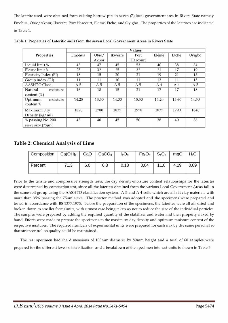
The laterite used were obtained from existing borrow pits in seven (7) local government area in Rivers State namely
Emohua, Obio/Akpor, Ikwerre, Port Harcourt, Eleme, Etche, and Oyigbo. The properties of the laterites are indicated
in Table 1.
Table 1: Properties of Lateritic soils from the seven Local Government Areas in Rivers State
Properties
Values
Emohua Obio/
Akpor
Ikwerre Port
Harcourt
Eleme Etche Oyigbo
Liquid limit % 43 47 45 53 40 38 34
Plastic limit % 25 32 25 32 21 17 19
Plasticity Index (PI) 18 15 20 21 19 21 15
Group index (GI) 11 11 10 11 13 11 15
AASHTO Class A-5 A-5 A-5 A-5 A-4 A-4 A-5
Natural moisture
content (%)
16 18 15 21 17 17 18
Optimum moisture content %
14.25 13.50 14.00 15.50 14.20 15.60 14.50
Maximum Dry
Density (kg/m3)
1820 1780 1835 1958 1835 1790 1840
% passing No. 200
sieve size (75n(
43 40 45 50 38 40 38
Table 2: Chemical Analysis of Lime
Prior to the tensile and compressive strength tests, the dry density-moisture content relationships for the laterites
were determined by compaction test, since all the laterites obtained from the various Local Government Areas fall in
the same soil group using the AASHTO classification system. A-5 and A-4 soils which are all silt clay materials with
more than 35% passing the 75m sieve. The proctor method was adopted and the specimens were prepared and
tested in accordance with BS 1377:1975. Before the preparation of the specimens, the laterites were all air dried and
broken down to smaller form/units, with utmost care being taken as not to reduce the size of the individual particles.
The samples were prepared by adding the required quantity of the stabilizer and water and then properly mixed by
hand. Efforts were made to prepare the specimens to the maximum dry density and optimum moisture content of the
respective mixtures. The required numbers of experimental units were prepared for each mix by the same personal so
that strict control on quality could be maintained.
The test specimen had the dimensions of 100mm diameter by 80mm height and a total of 60 samples were
prepared for the different levels of stabilization and a breakdown of the specimen into test units is shown in Table 3.
Composition Ca(OH)2 CaO CaCO3 l2O3 Fe2O3 S1O2 mgO H2O
Percent 71.3 6.0 6.3 0.18 0.04 11.0 4.19 0.09

D.B.Eme1IJECS Volume 3 Issue 4 April, 2014 Page No.5471-5494 Page 5475
Table 3: Break down of specimen into test units silty clay materials (A -5) soil
AGE (DAYS)
TEST METHOD LIME CONTENT (%)
7 14 21 28
Split Cylinder (SC)
0%
2%
3
3
3
3
3
3
3
3
4%
6%
8%
3
3
3
3
3
3
3
3
3
3
3
3
The specimens were moist cured for 7, 14, 21 and 28 days at constant moisture content and at laboratory temperature
of about 28oC. The specimens were stored in plastic containers with moist sawdust to prevent moisture loss during
curing period and to preserve the moulding as much as possible.The CBR machine was used for all tests
Brazilian Split-Cylinder Test
Figure 1: Brazilian split-cylinder test (i) Test (ii) arrangement
In the Brazilian split-cylinder test a compressive strip load was applied to the cylindrical specimen along two
opposite generators. This condition set up an almost uniform tensile stress over the vertical diametrical plane, and
fracture (splitting) of the specimen occurred along the loading plane (Figure 1). The indirect tensile strength at fai lure
is given as in equation 1
dt
Pt
2 (1)
Where;
P = load at failure in N
P
P
(i) test
(ii)

D.B.Eme1IJECS Volume 3 Issue 4 April, 2014 Page No.5471-5494 Page 5476
d = specimen diameter in mm
t = specimen thickness in mm
After obtaining the tensile strength of the material using the indirect tensile strength test methods. The
strains (vertical and horizontal) were measured using strain gauges Demec No. 3463 strain gauge, to load the
specimen the bearing strips were first positioned and aligned. The plunger of the CBR machine was then made to site
on upper bearing strip before the load gauge was set on zero. The strain measuring tags were attached to each of the
ends along the axes using super glue”. Load was continuously applied (With few seconds shock to allow for strain
gauging). The loading was done until failure load was obtained. Gage readings were taken at both ends so that the
average of two vertical and two horizontal strain measurements were determined for each increment of load, the
vertical and horizontal strains were recorded directly from Deme 3463 strain gage.Equations (1) was used to generate
the tensile strength of the soil-lime mixture for the indirect tensile strength testing technique used.
III. DEVELOPED MODELS FOR PREDICTING ELASTIC MODULUS USING SPSS
The following were the steps undertaken to develop the models that can be used to predict elastic modulus from
compressive modulus of lateritic soils stabilized with lime content;
1. Determine the elastic modulus of the soil mixture using the different indirect tensile testing techniques for the
various lime contents
2. Determine the compressive modulus of the soil mixture using the different indirect tensile testing techniques for
the various lime content
3. Obtain the logarithm of both elastic and compressive moduli for the different indirect tensile testing techniques
for the various lime content
4. Write a non-linear regression equation that satisfies the condition of the proposed general form of the elastic -
compressive model
5. Input stringed variables into the SPSS software for non linear analysis
Note: the proposed model is of the form;
b
MM CaEln435.0
2
Where;
EM = elastic modulus
CM = compressive modulus
a, b, c = experimentally determined co-efficient from non linear regression.
From equation 4.1, the logarithm form can be expressed as,
b
MM CaLogELogln435.0
)( 3

D.B.Eme1IJECS Volume 3 Issue 4 April, 2014 Page No.5471-5494 Page 5477
For convenience of use in the SPSS software the independent variable was expressed in the natural logarithm form.
That is,
b
MM CaLnELogln435.0
3.2
1)( 4
Developing Proposed Elastic - Compressive Moduli Models Using Non Linear Regression Approach in SPSS
A non linear model is one in which at least one of the parameters appear nonlinearly (Prajneshu, No Date). More
formally, in a nonlinear model, at least one derivative with respect to a parameter should involve that parameter. To
solve the non linear regression using SPSS the variables (dependent and independent) were first of all collated in to
different cells in the “Data View” dialogue box. Next these variables were stringed and coded into another dialogue
box called the “Variable View Cell”. Finally model syntax was developed that satisfies the condition of the general
form of the non linear model (Draper and Smith, 1998).
Non Linear Model Syntax
The non linear model syntax is of the form as shown below;
))ln*435.0*(*(**435.0 bCaLnY M 5
Where,
Y = dependent variable = Log (EM)
CM = independent variable
a and b are co-efficients to be determined from the non linear regression equation.
Equation 5 is the non linear syntax model that is synonymous with the general form of the proposed model used for
analysis in the SPSS program.
Finally, in SPSS the command (**) means raising a variable to the power of the coefficient in the same bracket while
the command (*) means multiplication.

D.B.Eme1IJECS Volume 3 Issue 4 April, 2014 Page No.5471-5494 Page 5478
IV RESULT AND DISCUSSION
Split Cylinder Test
Table 4: Variations @ 7 Days Curing
Lime Content (%) Compressive Modulus, CM
(MPa)
Elastic Modulus, E
(MPa)
0 1333.333 1100
2 1536.364 1253.521
4 2557.522 1506.998
6 2761.905 1735.219
8 2814.081 1887.805
Figure 2 : Split Cylinder Stiffness Variation with Lime Content @ 7 Days Curing
Table 5: Variations @ 14 Days Curing
Lime Content (%) Compressive Modulus, CM
(MPa) Elastic Modulus, E
(MPa)
0 1364.706 851.3514
2 2096.33 910.5691
4 2533.793 1578.488
6 2818.408 1764.331
8 2900 1982.885

D.B.Eme1IJECS Volume 3 Issue 4 April, 2014 Page No.5471-5494 Page 5479
Figure 3: Split Cylinder Stiffness Variation with Lime Content @ 14 Days Curing
Table 6: Variations @ 21 Days Curing
Lime Content (%) Compressive Modulus, CM
(MPa)
Elastic Modulus, E
(MPa)
0 1273.585 794.7368
2 1692.41 889.5582
4 2013.17 1569.604
6 2125 1748.466
8 2279.767 1775.201
Figure 4: Split Cylinder Stiffness Variation with Lime Content @ 21 Days Curing

D.B.Eme1IJECS Volume 3 Issue 4 April, 2014 Page No.5471-5494 Page 5480
Table 7: Variations @ 28 Days Curing
Lime Content (%) Compressive Modulus, CM
(MPa)
Elastic Modulus, E
(MPa)
0 1166.667 783.5052
2 1611.86 883.4842
4 1871.93 1456.763
6 1980.952 1621.711
8 2233.032 1945.931
Figure 5: Split Cylinder Stiffness Variation with Lime Content @ 28 Days Curing
variation of Elastic Modulus (Em) and compressive modulus (Cm) of lateritic soil
with lime content .
For the various ages of curing the elastic modulus was increasing with increasing lime content, this goes to show that
at 0% lime content the elastic modulus was low, but with the addition of lime it was increased see table(4 -7) and fig(2-
5) which means that lime increases the elastic modulus of lateritic soil. More so the tensile stress, compressive strain,
and tensile strain were all increasing with increasing lime content as in (table 8 -12), this finding is in line with Miller et
al (2006), Thompson(1989). However the increase in elastic modulus was linear up to the highest lime content of 8%
this could be as a result of the chemical reactions that took place during the process of stabilization, the addition of
lime supplied an excess Ca+2 which goes to replace the weaker metallic cat-ions from the exchange complex of the soil.
The exchange of this cat ions causes a reduction in the diffused water layer there by allowing clay particles to
approach each other closely or flocculate, this finding is in line with Little et al(1995) the same trend was observed for
all other ages of curing. Also the compressive modulus was increasing linearly with an increase in lime content,
though the compressive modulus was higher than elastic modulus as shown in the table (4 -7) and fig(2-5), This shows
that compressive modulus is a very important parameter in the soil which is to be used as a pavement material, the
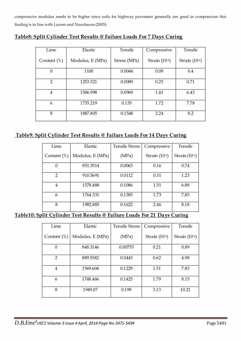
D.B.Eme1IJECS Volume 3 Issue 4 April, 2014 Page No.5471-5494 Page 5481
compressive modulus needs to be higher since soils for highway pavement generally are good in compression this
finding is in line with Larsen and Nussbaum (2005).
Table8: Split Cylinder Test Results @ Failure Loads For 7 Days Curing
Lime
Content (%)
Elastic
Modulus, E (MPa)
Tensile
Stress (MPa)
Compressive
Strain (10-4)
Tensile
Strain (10-4)
0 1100 0.0044 0.08 0.4
2 1253.521 0.0089 0.25 0.71
4 1506.998 0.0969 1.41 6.43
6 1735.219 0.135 1.72 7.78
8 1887.805 0.1548 2.24 8.2
Table9: Split Cylinder Test Results @ Failure Loads For 14 Days Curing
Lime
Content (%)
Elastic
Modulus, E (MPa)
Tensile Stress
(MPa)
Compressive
Strain (10-4)
Tensile
Strain (10-4)
0 851.3514 0.0063 0.16 0.74
2 910.5691 0.0112 0.31 1.23
4 1578.488 0.1086 1.51 6.88
6 1764.331 0.1385 1.73 7.85
8 1982.885 0.1622 2.46 8.18
Table10: Split Cylinder Test Results @ Failure Loads For 21 Days Curing
Lime
Content (%)
Elastic
Modulus, E (MPa)
Tensile Stress
(MPa)
Compressive
Strain (10-4)
Tensile
Strain (10-4)
0 848.3146 0.00755 0.21 0.89
2 889.5582 0.0443 0.62 4.98
4 1569.604 0.1229 1.51 7.83
6 1748.466 0.1425 1.79 8.15
8 1949.07 0.199 3.13 10.21

D.B.Eme1IJECS Volume 3 Issue 4 April, 2014 Page No.5471-5494 Page 5482
Table11: Split Cylinder Test Results @ Failure Loads For 28 Days Curing
Lime
Content (%)
Elastic
Modulus, E (MPa)
Tensile Stress
(MPa)
Compressive
Strain (10-4)
Tensile
Strain (10-4)
0 783.5052 0.0076 0.21 0.97
2 883.4842 0.0781 1.01 8.84
4 1456.763 0.1314 1.7 9.02
6 1621.711 0.1479 2.01 9.12
8 1945.931 0.3491 3.93 17.94
Table 12:Split Cylinder Test Calibration for Lime – Lateritic Soil Mixture
@ 7 Days Curing
Lime
Content (%)
Compressive
Modulus, CM
(MPa)
Log CM
(MPa)
Elastic
Modulus, E
(MPa)
Log E
(MPa)
0 1333.333 3.124939 1100 3.041393
2 1536.364 3.186494 1253.521 3.098132
4 2557.522 3.407819 1506.998 3.178113
6 2761.905 3.441209 1735.219 3.239354
8 2814.081 3.449337 1887.805 3.275957
By applying equation 5 in the SPSS program, the experimental co-efficients were determined from table 1a(ii) is
as follows;
a = 12.793; b = 4.16; [See appendix A: Table 1a (i)]
The resulting prediction model equation in syntax form becomes;
))6.4ln*435.0*(*(*793.12*435.0 MCLnY 6
Since Y = Log (EM), the actual prediction model equation can be written as;
b
MM CLogLogEln435.0
793.12 7

D.B.Eme1IJECS Volume 3 Issue 4 April, 2014 Page No.5471-5494 Page 5483
16.4ln435.0)(793.12435.0
10 MCLn
ME 8
Equation 8 can be used to predict elastic modulus of lime – lateritic soil mixtures cured at 7 days curing for given
compressive modulus with a correlation value of R2 = 0.903.
Table 13:Split Cylinder Test Calibration for Lime – Lateritic Soil Mixture
@ 14 Days Curing
Lime
Content (%)
Compressive
Modulus, CM
(MPa)
Log CM
(MPa)
Elastic
Modulus, E
(MPa)
Log E
(MPa)
0 1364.706 3.135039 851.3514 2.930109
2 2096.33 3.32146 910.5691 2.959313
4 2533.793 3.403771 1578.488 3.198241
6 2818.408 3.450004 1764.331 3.24658
8 2900 3.462398 1982.885 3.297298
By applying equation 5 in the SPSS program, the experimental co-efficients were determined from table (2aii) is as
follows;
a = 0.025; b = 25.399; [See appendix A: Table 2a (i)]
The resulting prediction model equation in syntax form becomes;
))399.25ln*435.0*(*(*025.0*435.0 MCLnY 9
Since Y = Log (EM), the actual prediction model equation is can be written as;
399.25ln435.0025.0 MM CLogLogE 10
399.25ln435.0)(025.0435.0
10 MCLn
ME 11
Equation 11 can be used to predict elastic modulus of lime – lateritic soil mixtures cured at 14 days curing for given
compressive modulus with a correlation value of R2 = 0.874.
Table 14:Split Cylinder Test Calibration for Lime – Lateritic Soil Mixture
@ 21 Days Curing

D.B.Eme1IJECS Volume 3 Issue 4 April, 2014 Page No.5471-5494 Page 5484
Lime
Content (%)
Compressive
Modulus, CM
(MPa)
Log CM
(MPa)
Elastic
Modulus, E
(MPa)
Log E
(MPa)
0 1273.585 3.105028 848.3146 2.928557
2 1692.41 3.228506 889.5582 2.949174
4 2013.17 3.30388 1569.604 3.19579
6 2125 3.327359 1748.466 3.242657
8 2279.767 3.35789 1949.07 3.289827
By applying equation 5 in the SPSS program, the experimental co-efficients were determined from table (3aii) is as
follows;
a = 0.003; b = 51.401; [See appendix A: Table 3a (i)]
The resulting prediction model equation in syntax form becomes;
))401.51ln*435.0*(*(*003.0*435.0 MCLnY 12
Since Y = Log (EM), the actual prediction model equation is can be written as;
401.51ln435.0003.0 MM CLogLogE 13
401.51ln435.0)(03.0435.0
10 MCLn
ME 14
Equation 14 can be used to predict elastic modulus of lime – lateritic soil mixtures cured at 21 days curing for given
compressive modulus with a correlation value of R2 = 0.907
Table 15:Split Cylinder Test Calibration for Lime – Lateritic Soil Mixture
@ 28 Days Curing
Lime
Content (%)
Compressive
Modulus, CM
(MPa)
Log CM
(MPa)
Elastic
Modulus, E
(MPa)
Log E
(MPa)
0 1166.667 3.066947 783.5052 2.894042
2 1611.86 3.207327 883.4842 2.946199
4 1871.93 3.27229 1456.763 3.163389
6 1980.952 3.296874 1621.711 3.209973
8 2233.032 3.348895 1945.931 3.289127

D.B.Eme1IJECS Volume 3 Issue 4 April, 2014 Page No.5471-5494 Page 5485
By applying equation 5 in the SPSS program, the experimental co-efficients were determined from table ( 4aii) is
as follows;
a = 0.003; b = 52.165; [See appendix A: Table 4a (i)]
The resulting prediction model equation in syntax form becomes;
))165.52ln*435.0*(*(*003.0*435.0 MCLnY 15
Since Y = Log (EM), the actual prediction model equation is can be written as;
165.52ln435.0003.0 MM CLogLogE 16
165.52ln435.0)(03.0435.0
10 MCLn
ME 17
Equation 17 can be used to predict elastic modulus of lime – lateritic soil mixtures cured at 28 days curing for given
compressive modulus with a correlation value of R2 = 0.924.
Verification of derived model for split cylinder test for lime lateritic soil mixture
Table 16: 7 Days Curing
Lime Content(%) CM EM(Measured) EM(Predicted)
0 1333.333 1100 1108.428
2 1536.364 1253.521 1207.67
4 2557.522 1506.998 1643.805
6 2761.905 1735.219 1722.07
8 2814.081 1887.805 1741.679
The predicted EM values was obtained by applying equation 8 while the measured was obtained from lab
theL laboratory

D.B.Eme1IJECS Volume 3 Issue 4 April, 2014 Page No.5471-5494 Page 5486
Figure :6 Prediction of Elastic Modulus from compressive strength using SC @ 7DAYS
Verification of derived model for split cylinder test for lime lateritic soil mixture
Table 17: 14 Days Curing
Lime Content(%) CM EM(Measured) EM(Predicted)
0 1364.706 851.3514 750.2398
2 2096.33 910.5691 1219.63
4 2533.793 1578.488 1511.488
6 2818.408 1764.331 1705.062
8 2900 1982.885 1761.045
The predicted EM values was obtained by applying equation 11 while the measured was obtained from the laboratory.
Figure:7 Prediction of Elastic Modulus from compressive strength using SC @ 14 days
Verification of derived model for split cylinder test for lime lateritic soil mixture
Table 18: 21 Days Curing
Lime Content (%) CM EM (Measured) EM (Predicted)
0 1364.706 851.3514 750.2398
2 2096.33 910.5691 1219.63
4 2533.793 1578.488 1511.488
6 2818.408 1764.331 1705.062
8 2900 1982.885 1761.045
The predicted EM values were obtained by applying equation 14 while the
measured was obtained from the laboratory.

D.B.Eme1IJECS Volume 3 Issue 4 April, 2014 Page No.5471-5494 Page 5487
Figure:8 Prediction of Elastic Modulus from compressive strength using SC @ 21 days
Verification of derived model for split cylinder test for lime lateritic soil mixture
Table 19: 28 Days Curing
Lime Content (%) CM EM (Measured) EM (Predicted)
0 1166.667 783.5052 701.4001
2 1611.86 883.4842 1129.866
4 1871.93 1456.763 1408.79
6 1980.952 1621.711 1531.47
8 2233.032 1945.931 1827.424
The predicted EM values was obtained by applying equation 17 while the measured was obtained from the laboratory.
Figure:9 Prediction of Elastic Modulus from compressive strength using SC @ 28 days

D.B.Eme1IJECS Volume 3 Issue 4 April, 2014 Page No.5471-5494 Page 5488
Verification of derived Predictive Models
Part of the work was devoted to the verification of the derived models developed by comparison with measured
values. The method of verification was done through the use of multiple correlations by determining R 2 values as
shown in the graphical plots, fig(6-9) the determination of R2 was found to be very good with an average of 92% and
above recalling that the model prediction for the elastic modulus is ok, since in highway engineering Elastic modulus
is very essential mainly in the sub-base layer of the pavement.
V. CONCLUSIONS
The following conclusions can be drawn from this study
1. The Elastic and Compressive modulus increases with an increase in lime content up to 8% lime content.
2. The predicted values were close to the measured values with an average R2 value of 92%
3. The models developed from this work can be used to predict Elastic modulus from compressive
modulus using the Split cylinder at different days of curing using lime.
4. The predicted Elastic Modulus can be used for the Mechanistic design of pavement.
LIST OF ITERATION TABLES USED FOR CALIBRATION OF LIME-LATERITIC SOIL
MIXTURE FOR SPLIT CYLINDER
Table 1a (i): Iteration History for 7Days Curing
Iteration Number(a) Residual Sum of
Squares
Parameter
a b
0.1 11587515.216 14.260 .605
1.1 41548.360 14.303 4.025 2.1 41548.032 14.295 4.025 3.1 41458.156 13.584 4.085 4.1 41419.791 13.538 4.090
5.1 41387.877 13.097 4.130 6.1 41376.761 13.022 4.138 7.1 41372.959 12.830 4.156 8.1 41372.211 12.819 4.158 9.1 41372.154 12.795 4.160
10.1 41372.153 12.793 4.160 11.1 41372.153 12.793 4.160
Derivatives are calculated numerically. a. Major iteration number is displayed to the left of the decimal, and minor iteration number is to the
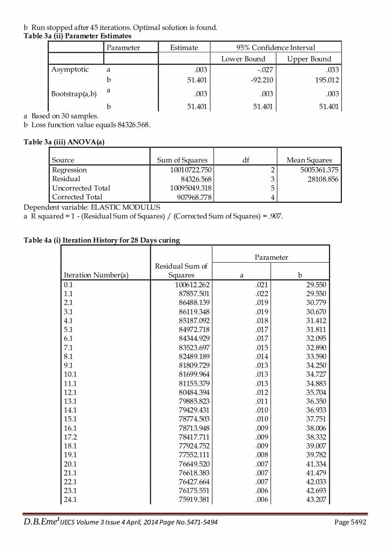
right of the decimal. b. Run stopped after 11 iterations. Optimal solution is found.

D.B.Eme1IJECS Volume 3 Issue 4 April, 2014 Page No.5471-5494 Page 5489
Table 1a (ii) Parameter Estimates
Parameter Estimate 95% Confidence Interval
Lower Bound Upper Bound
Asymptotic a 12.793 -27.261 52.846
b 4.160 .303 8.017
Bootstrap(a,b) a 12.793 12.793 12.793
b 4.160 4.160 4.160 a Based on 30 samples. b Loss function value equals 41372.153.
Table 1a (iii) ANOVA
Source Sum of Squares df Mean Squares
Regression 11585777.907 2 5792888.954
Residual 41372.153 3 13790.718
Uncorrected Total 11627150.060 5
Corrected Total 426467.017 4
Dependent variable: ELASTIC MODULUS a R squared = 1 - (Residual Sum of Squares) / (Corrected Sum of Squares) = .903. Table 2a (i) Iteration History for 14 Days Curing
Iteration Number(a)
Residual Sum of Squares Parameter
a b
0.1 156489.898 .212 13.550 1.1 155705.343 .217 13.550
2.1 151304.385 .183 14.178 3.2 151280.085 .181 14.217 4.1 150855.677 .179 14.286 5.1 149341.506 .158 14.783 6.1 147824.859 .155 14.915
7.1 146532.955 .142 15.282 8.1 146233.271 .136 15.461 9.1 145021.582 .130 15.679 10.1 143867.609 .121 16.021
11.1 142501.406 .112 16.435 12.1 141533.655 .101 16.884 13.1 141327.555 .104 16.759 14.1 140860.916 .100 16.936
15.1 140466.554 .095 17.186 16.1 140084.836 .093 17.320 17.1 138960.963 .087 17.672 18.1 138596.988 .083 17.910 19.1 138210.524 .079 18.157
20.1 137283.998 .074 18.476 21.1 136999.360 .071 18.738 22.1 136210.079 .066 19.151 23.1 136053.327 .064 19.332
24.1 135138.509 .059 19.743 25.1 135094.580 .058 19.844 26.1 134908.154 .057 19.949

D.B.Eme1IJECS Volume 3 Issue 4 April, 2014 Page No.5471-5494 Page 5490
27.1 134383.941 .054 20.343 28.1 133961.010 .051 20.637 29.1 133693.751 .048 20.943
30.1 133559.193 .047 21.127 31.1 133113.498 .044 21.484 32.1 132987.836 .043 21.735 33.1 132625.296 .040 22.181
34.1 132505.757 .040 22.232 35.1 132313.823 .037 22.633 36.1 132222.958 .037 22.719 37.1 132144.077 .035 22.979 38.1 131934.775 .034 23.229
39.2 131883.979 .033 23.436 40.1 131794.074 .032 23.627 41.1 131699.669 .031 23.818 42.1 131632.176 .030 24.134
43.1 131602.282 .030 24.128 44.1 131538.752 .029 24.384 45.1 131508.925 .028 24.597 46.2 131458.391 .027 24.763
47.1 131442.473 .027 24.933 48.1 131410.295 .026 25.109 49.1 131395.263 .026 25.251 50.1 131384.541 .025 25.399
Derivatives are calculated numerically.
a Major iteration number is displayed to the left of the decimal, and minor iteration number is to the right of the decimal. b Run stopped after 50 iterations because it reached the limit for the number of iterations. Table 2a (ii) Parameter Estimates
Parameter Estimate 95% Confidence Interval
Lower Bound Upper Bound
Asymptotic a .025 -.214 .264
b 25.399 -45.085 95.883
Bootstrap(a,b) a
.025 -.154 .204
b 25.399 13.285 37.514 a Based on 30 samples. b Loss function value equals 131384.541.
Table 2a (iii) ANOVA
Source Sum of Squares df Mean Squares
Regression 10958874.102 2 5479437.051
Residual 131384.541 3 43794.847 Uncorrected Total 11090258.643 5
Corrected Total 1043372.660 4
Dependent variable: ELASTIC MODULUS
a R squared = 1 - (Residual Sum of Squares) / (Corrected Sum of Squares) = .874.
Table 3a (i) Iteration History for 21 Days Curing

D.B.Eme1IJECS Volume 3 Issue 4 April, 2014 Page No.5471-5494 Page 5491
Iteration Number(a)
Residual Sum of Squares Parameter
A b
0.1 90086.066 .010 36.480 1.1 88618.544 .010 36.480 2.1 88188.492 .009 37.166
3.1 88083.668 .009 37.679 4.1 87826.254 .009 37.778 5.2 87416.891 .008 38.564 6.1 87074.229 .008 39.143 7.1 86775.360 .008 39.686
8.1 86492.322 .007 40.405 9.1 86389.416 .007 40.611 10.2 86124.202 .007 41.215 11.1 85864.900 .006 41.922
12.1 85802.386 .006 42.195 13.1 85505.683 .006 42.974 14.1 85355.107 .006 43.385 15.1 85280.840 .006 43.825 16.1 85184.865 .005 44.246
17.1 85002.741 .005 44.789 18.1 84939.868 .005 45.339 19.1 84880.406 .005 45.434 20.1 84809.033 .005 46.327
21.1 84728.890 .005 46.216 22.1 84665.543 .004 46.627 23.2 84636.679 .004 46.982 24.1 84606.647 .004 47.179
25.2 84529.930 .004 47.649 26.1 84509.205 .004 48.051 27.1 84477.795 .004 48.218 28.1 84456.089 .004 48.880 29.1 84414.191 .004 48.929
30.1 84388.554 .004 49.329 31.1 84383.282 .004 49.543 32.1 84372.157 .004 49.682 33.1 84354.210 .004 50.020
34.1 84343.881 .003 50.333 35.1 84340.667 .003 50.677 36.1 84329.487 .003 51.161 37.1 84328.281 .003 51.066 38.1 84327.914 .003 51.099
39.1 84326.843 .003 51.287 40.1 84326.629 .003 51.340 41.1 84326.573 .003 51.390 42.1 84326.569 .003 51.397
43.1 84326.568 .003 51.402 44.1 84326.568 .003 51.401 45.1 84326.568 .003 51.401
Derivatives are calculated numerically. a Major iteration number is displayed to the left of the decimal, and minor iteration number is to the right
of the decimal.
D.B.Eme1IJECS Volume 3 Issue 4 April, 2014 Page No.5471-5494 Page 5492
b Run stopped after 45 iterations. Optimal solution is found. Table 3a (ii) Parameter Estimates
Parameter Estimate 95% Confidence Interval
Lower Bound Upper Bound
Asymptotic a .003 -.027 .033
b 51.401 -92.210 195.012
Bootstrap(a,b) a
.003 .003 .003
b 51.401 51.401 51.401
a Based on 30 samples. b Loss function value equals 84326.568. Table 3a (iii) ANOVA(a)
Source Sum of Squares df Mean Squares
Regression 10010722.750 2 5005361.375 Residual 84326.568 3 28108.856 Uncorrected Total 10095049.318 5 Corrected Total 907968.778 4
Dependent variable: ELASTIC MODULUS a R squared = 1 - (Residual Sum of Squares) / (Corrected Sum of Squares) = .907.
Table 4a (i) Iteration History for 28 Days curing
Iteration Number(a) Residual Sum of
Squares
Parameter
a b
0.1 100612.262 .021 29.550 1.1 87857.501 .022 29.550 2.1 86488.139 .019 30.779
3.1 86119.348 .019 30.670 4.1 85187.092 .018 31.412 5.1 84972.718 .017 31.811 6.1 84344.929 .017 32.095
7.1 83523.697 .015 32.890 8.1 82489.189 .014 33.590 9.1 81809.729 .013 34.250 10.1 81699.964 .013 34.727
11.1 81155.379 .013 34.883 12.1 80484.394 .012 35.704 13.1 79885.823 .011 36.350 14.1 79429.431 .010 36.933 15.1 78774.503 .010 37.751
16.1 78713.948 .009 38.006 17.2 78417.711 .009 38.332 18.1 77924.752 .009 39.007 19.1 77552.111 .008 39.782
20.1 76649.520 .007 41.334 21.1 76618.383 .007 41.479 22.1 76427.664 .007 42.033 23.1 76175.551 .006 42.693 24.1 75919.381 .006 43.207

D.B.Eme1IJECS Volume 3 Issue 4 April, 2014 Page No.5471-5494 Page 5493
25.1 75713.929 .006 43.992 26.2 75641.108 .006 44.023 27.1 75458.666 .005 44.981
28.1 75329.921 .005 45.073 29.1 75195.955 .005 45.949 30.1 75113.031 .005 45.999 31.1 74998.496 .005 46.873
32.2 74921.803 .005 46.949 33.1 74838.711 .004 47.783 34.1 74784.165 .004 47.794 35.1 74711.122 .004 48.435 36.1 74680.019 .004 48.965
37.1 74612.616 .004 49.221 38.1 74581.714 .004 49.699 39.1 74563.663 .004 49.996 40.1 74526.887 .004 50.378
41.1 74514.210 .004 50.726 42.2 74506.208 .004 50.901 43.1 74492.605 .004 51.191 44.1 74486.208 .003 51.503
45.1 74483.562 .003 51.590 46.1 74479.635 .003 51.844 47.1 74478.622 .003 51.888 48.2 74477.523 .003 52.127 49.1 74477.273 .003 52.107
50.1 74477.153 .003 52.165
Derivatives are calculated numerically. a Major iteration number is displayed to the left of the decimal, and minor iteration number is to the right of the decimal.
b Run stopped after 50 iterations because it reached the limit for the number of iterations.
Table 4a (ii) Parameter Estimates
Parameter Estimate 95% Confidence Interval
Lower Bound Upper Bound
Asymptotic a .003 -.024 .030
b 52.165 -75.391 179.721
Bootstrap(a,b) a .003 -.016 .023
b 52.165 29.420 74.909 a Based on 30 samples.
b Loss function value equals 74477.153. Table 4a (iii) ANOVA
Source Sum of Squares df Mean Squares
Regression 9858697.171 2 4929348.586
Residual 74477.153 3 24825.718
Uncorrected Total 9933174.324 5
Corrected Total 978225.001 4
Dependent variable: ELASTIC MODULUS a R squared = 1 - (Residual Sum of Squares) / (Corrected Sum of Squares) = .924.
REFERENCES

D.B.Eme1IJECS Volume 3 Issue 4 April, 2014 Page No.5471-5494 Page 5494
(1)Bridges, E.M. (1970). World soils Cambridge, university press London, p25.
(2)Fookes G. (1997). Tropical residual soils, a geological society engineering group working party reused report. The geological society, London.
(3)Lambe T.W. and Whitman, V.R. (1979), Soil mechanics, diversion John Wiley and sons Inc. New York.
(4) Makasa B. (2004), Utilization and improvement of lateritic gravels in road bases, international institute for
aerospace survey and earth sciences, Delft.
(5) Mamlouk, M.S. and Wood, L.E.” (1981). Characterization of Asphalt Emulsion Treated Bases” ASCE Journal of Transportation Division, Vol. 107, No. TE2, pp. 183-196
(6) Thagesen B. (1996) Tropical rocks and soils in highway and traffic engineering in developing countries. Thagesen B. ed. Chapman and Hall, London.
(7) AASHTO Interim Guide for Design of Pavement Structures,’ American Association of State Highway and
Transportation Officials, 1972, chapter III revised, 1981 (8)Baladi, G. Y., Characterization of Flexible Pavement: A Case Study, American Society for Testing and Material,
Special Technical Paper No. 807, 1983, p 164-171
(9)Kenis, W. J., I’Material Characterizations for Rational Pavement Design, ‘1 American Society for Testing and
Material, Special Technical Paper No. 561, 1973, p 132-152.
(10) Mamlouk S. Micheal and Sarofim T. Ramsis, ‘The Modulus of Asphalt Mixtures - An Unresolved Dilemma, Transportation Research Board, 67th annual meeting, 1998.
(11) AASHTO Test and Material Specifications, Parts I and II, 13th edition, American Association for State Highway and Transportation Official, 1982.
(12) Scott, J.L.M, Flexural stress-strain characteristics of Saskatchewan soil cements, Technical Report 23,Saskatchewan
Department of Highways and Transportation, Canada, 1974.
(13) Pretorius, P. C and Monismith, C.L, “The prediction of shrinkage stresses in pavements containing soil cement Bases” Paper presented at the annual meeting of the Highway Research Board, Washington D.C,1971
(14) Packard, R.G “Structural Design of concrete pavements with lean concrete lower course”2 nd Rigid Pavement
Conference, Purdue University 1981.
(15)Lilley A.A Cement stabilized material in Great Britain, Record 422, Highway Research Board 1973.
(16) Felt. E. J and Abrams M.S Strength and Elastic properties of compacted soil-cement Mixtures, special Technical Publications Number 206, American Society for Testing Materials,2008.
(17) Larsen T.J. and Nussbaum, P.J Fatigue of soil cement, Bulletin D119 Portland cement Association,2005
(18) Jones .R. Measurement of Elastic and strength properties of ce mented materials in Road Bases, Reord 128
Highway Research Board 2007
(19) Schen.C.K. “Behaviour of Cement Stabilized Soils Under Repeated Loading,” Ph.D Dissertation, Department of
civil Engineering, University of California, Berkeley 1965.
(20) Wang,M.C Stress and Deflection in Cement-Stabilized Soil Pavements Ph.D Dissertation, University of California
Berkeley 1968.
(21) Mitchel, J. K, Fossberg. P.E, and Monismith, C. L. Behaviour of stabilized Soils Under Repeated Loading, Report3:
Repeated Compression and Flexure Tests on Cement and Lime Treated Buckshot Clay, Confining Pressure Effects in
Reapeted Compression for Cement Treated Silty Clay, Contract Report 3-145, U.S. Army Engineer Waterways Experiment Station,1969.
(22) SPSS 2005.SPSS Windows Evaluation, Release 14.00.SPSS INC, Chika