Simulation of Lime Calcination in Normal Shaft and Parallel ...

Simulation of Lime Calcination in Normal Shaft and Parallel Flow

Regenerative Kilns

Dissertation

zur Erlangung des Akademischen Grades

Doktoringenieur (Dr.-Ing.)

von: M.Sc. Duc Hai Do geb. am: 15.03.1979 in: Vinh Phuc / Viet Nam genehmigt durch die Fakultät für Verfahrens- und Systemtechnik der Otto-von-Guericke-Universität Magdeburg Gutachter: Prof. Dr.-Ing. Eckehard Specht

Prof. Dr.-Ing. Roman Weber Dr.-Ing. Georg Kehse

Promotionskolloquium am: 25.04.2012

i

Schriftliche Erklärung Ich erkläre hiermit, dass ich die vorliegende Arbeit ohne unzulässige Hilfe Dritter und ohne Benutzung anderer als der angegebenen Hilfsmittel angefertigt habe. Die aus fremden Quellen direkt oder indirekt übernommenen Gedanken sind als solche kenntlich gemacht. Insbesondere habe ich nicht die Hilfe einer kommerziellen Promotionsberatung in Anspruch genommen. Dritte haben von mir weder unmittelbar noch mittelbar geldwerte Leistungen für Arbeiten erhalten, die im Zusammenhang mit dem Inhalt der vorgelegten Dissertation stehen. Die Arbeit wurde bisher weder im Inland noch im Ausland in gleicher oder ähnlicher Form als Dissertation eingereicht und ist als Ganzes auch noch nicht veröffentlicht. Magdeburg, den 25.04.2012 Duc Hai Do

ii

Acknowledgements First and foremost, i would like to express my deep and sincere gratitude to my supervisor Prof. Dr.-Ing. Eckehard Specht, for his constant advice, encouragement and financial support. His strong motivation, creativity and rich knowledge and experience enriched my confidence level to solve many complex problems in effective ways. Furthermore, his friendly personality and patience have benefited me immensely.

I am deeply grateful to Prof. Dr.-Ing . Roman Weber from the Technische Universität Clausthal for his in-depth review of my dissertation and constructive comments.

I am deeply grateful to Dr. Georg Kehse from IWP Ingenieurbüro für Wärme und Prozesstechnik GmbH, who has been also working with me since the beginning of my Ph.D time, for his friendly guidance with rich industrial experiences.

Additional thanks are also grateful sent to Dr. Ferri, Mr. Christiansen and Mr. Bresciani from Cimprogetti S.p.A, Dalmine / Italy, for their kind / friendly helps during my work. I whole heartedly thank my colleagues Nadine, Magda, Fabian, Ping, Dr. Ashok, Dr. Woche, Dr. Al-Karawi, Gourisankar, Hassan, Hassanein, Khalid, Alfakheri, Pavan, Kotesvara Rao and of course, our friendly and warm-hearted secretary Christin Hasemann. My deepest gratitude goes to my family, including my wife Hue Chi, our ‘kleine diamond’ Lora - Bao Han, my mum and all of sisters and brothers, for their unflagging love and support throughout my life; this dissertation is simply impossible without them.

http://www.google.de/url?sa=t&rct=j&q=tu%20clausthal&source=web&cd=8&ved=0CC0QoAIwBw&url=http%3A%2F%2Fwww.tu-clausthal.de%2F&ei=n1-yT8vNKcb2sgbZ1ZmmBA&usg=AFQjCNHmpQy6TpjaMwR56BMz3bj5-bJypA&cad=rja

http://www.google.de/url?sa=t&rct=j&q=tu%20clausthal&source=web&cd=8&ved=0CC0QoAIwBw&url=http%3A%2F%2Fwww.tu-clausthal.de%2F&ei=n1-yT8vNKcb2sgbZ1ZmmBA&usg=AFQjCNHmpQy6TpjaMwR56BMz3bj5-bJypA&cad=rja

iii

Abstract Shaft kilns are widely used for the production of lime. For the purpose of process optimization (reducing energy consumption) and regulation (producing desired lime quality), the temperature and the lime burning profiles in the kilns must be known. However, practical measurements of these parameters are very difficult due to the movements of solid bed and high temperatures in the kilns. Therefore, it is important to determine these parameters by simulations. In this dissertation, mathematical models are developed to simulate the lime burning process in shaft kilns, focusing on normal shaft kilns and parallel flow regenerative (PFR) kilns. The mathematical models are one-dimensional and steady state, which describe the mass and energy conservations of the gas and the solid phases by a system of ordinary differential equations. A shrinking core model is employed to describe the mechanisms and to calculate the decomposition process of limestone particles. The models are used to determine significant parameters regarding the lime burning process such as: a) the core and surface temperatures of the solid (limestone / lime) particles, b) the gas temperature, c) the lime calcination degree or the residual CO2, d) the pressure drop along the kiln height and e) the heat loss by kiln wall. The models are also used to investigate variables that affect the lime burning process. The following variables have been investigated in detail by the models: a) energy consumption, b) kiln throughput, c) particle size, d) limestone origin, e) excess air number, f) fuel combustion behavior and g) solid bed height. Observations from simulation results figure out that the maximum temperatures of solid particles in the PFR kilns are significantly lower than that in the normal shaft kilns. In the PFR kilns, they vary in the range of 1000 – 1100 oC while in the normal shaft kilns they are in the range of 1400 – 1500 oC. In addition, to support mathematical modeling, theoretical minimum values of the specific energy consumption were determined. It has been observed that with the PFR kilns, as a result of reusing flue gas for regenerative heat transfer (saving energy), the energy consumption required for this type of kilns is significantly lower than that of the normal shaft kilns. The simulated results were validated by experiments with measuring temperature profiles in industrial shaft kilns. The measured temperatures are close to the solid temperature predicted by the models. The simulated and measured results are in good agreement. Keywords: Normal shaft kilns, PFR kilns, Modeling and Simulations, Measurements, Lime calcination, Temperature profile.

iv

Zusammenfassung Schachtöfen werden häufig für die Herstellung von Kalk verwendet. Zur Prozessoptimierung (Reduzierung des Energieverbrauchs) und zur Regulierung (Herstellung gewünschter Kalkqualität) müssen die Temperatur- und Kalkverbrennungsprofile in den Öfen bekannt sein. Allerdings sind praktische Messungen dieser Parameter sehr schwierig, aufgrund der Bewegung des Festbettes und den hohen Temperaturen in den Öfen. Daher ist es wichtig, diese Parameter durch Simulationen zu bestimmen. In dieser Dissertation wurden mathematische Modelle entwickelt, um den Kalkbrennprozess in Schachtöfen zu simulieren, insbesondere normaler Schachtöfen und Gleichstrom-Regenerativ-Schachtöfen (GGR-Öfen). Die entwickelten mathematischen Modelle sind eindimensional, stationär und beschreiben die Massen- und Energieerhaltung der Gas- und Feststoffphase durch ein System von gewöhnlichen Differentialgleichungen. Ein Schale-Kern-Modell wurde verwendet, um die Mechanismen zu beschreiben und den Zersetzungsprozess von Kalksteinpartikeln zu berechnen. Unter Verwendung der Modelle wurden wichtige Parameter in Bezug auf den Kalkbrennprozess in den Öfen bestimmt, wie a) die Kern- und Oberflächentemperaturen der Feststoffpartikel (Kalkstein / Kalk), b) die Gastemperatur, c) der Kalzinierungsgrad oder der Rest-CO2 Gehalt im Kalk, d) der Druckverlust über der Ofenhöhe und e) der Wärmeverlust durch die Ofenwand. Ebenso konnten mit Hilfe der Modelle Parameter untersucht werden, welche den Kalkbrennprozess beeinflussen. Die folgenden Parameter wurden von den Modellen näher untersucht: a) Energieverbrauch, b) Durchsatz im Ofen, c) Partikelgröße, d) Herkunft des Kalksteins, e) Luftzahl, f) Brennverhalten der Brennstoffe und g) Festbetthöhe. Betrachtungen der simulierten Ergebnisse zeigten, dass die maximalen Temperaturen der Feststoffpartikel in den GGR-Schachtöfen bedeutend niedriger sind als in den normalen Schachtöfen. In den GGR-Schachtöfen variieren die Temperaturen in einem Bereich von 1000-1100 °C während in den normalen Schachtöfen die Temperaturen im Bereich von 1400-1500 °C liegen. Zusätzlich wurden, zur Unterstützung der mathematischen Modellierung, theoretische Minimalwerte des spezifischen Energieverbrauchs ermittelt. Es wurde deutlich, dass aufgrund der Wiederverwendung des Rauchgases für die regenerative Wärmeübertragung (Energieeinsparung) der Energieverbrauch des GGR-Schachtofen bedeutend geringer ist als für den normalen Schachtofen. Die simulierten Ergebnisse wurden durch experimentelle Messungen von Temperaturprofilen in industriellen Schachtöfen validiert. Die gemessenen Temperaturen entsprechen annähernd der Feststofftemperatur, welche von den Modellen prognostiziert wurde. Die simulierten und gemessenen Ergebnisse stimmen gut überein. Schlagwörter: Normale Schachtöfen, GGR Öfen, Modellierung und Simulationen, Messungen, Kalzinierung, Temperaturprofil.

v

Table of contents

1 Introduction ........................................................................................................... 1 1.1 Overview and motivation ........................................................................................ 1 1.2 Lime production ...................................................................................................... 3 1.3 Lime shaft kilns ....................................................................................................... 4 1.4 Normal shaft kilns ................................................................................................... 5 1.5 PFR shaft kilns ........................................................................................................ 5

2 General description of sub-processes ................................................................ 11 2.1 Determination of heat transfer coefficient ............................................................. 11

2.1.1 Convective heat transfer coefficient ...................................................................... 11 2.1.2 Overall heat transfer coefficient ............................................................................ 12

2.2 Determination of mass transfer coefficient ........................................................... 12 2.3 Gas mixture properties .......................................................................................... 13 2.4 Flow pattern in packed bed ................................................................................... 15

2.4.1 Void fraction .......................................................................................................... 15 2.4.2 Pressure drop ......................................................................................................... 18

3 Decomposition of limestone ................................................................................ 20 3.1 Limestone characterization .................................................................................... 20 3.2 Lime quality .......................................................................................................... 20

3.2.1 Lime reactivity ...................................................................................................... 20 3.2.2 Residual CO2 in lime ............................................................................................. 22

3.3 Limestone decomposition model ........................................................................... 23 3.4 Determination of material properties .................................................................... 26

4 Energy and mass balance.................................................................................... 30 4.1 Energy and mass balance of normal shaft kiln ...................................................... 30

4.1.1 Process description ................................................................................................ 30 4.1.2 Energy balance ...................................................................................................... 30 4.1.3 Mass balance of CO2 ............................................................................................. 33 4.1.4 Equilibrium temperature ........................................................................................ 34 4.1.5 Energy consumption .............................................................................................. 35

4.2 Energy and mass balance of PFR kiln ................................................................... 38 4.2.1 Process description ................................................................................................ 38 4.2.2 Energy balance ...................................................................................................... 39 4.2.3 Mass balance of CO2 ............................................................................................. 42 4.2.4 Equilibrium temperature ........................................................................................ 43 4.2.5 Energy consumption .............................................................................................. 45

4.3 Conclusions ........................................................................................................... 49

5 Simulation of lime calcination in normal shaft kiln ......................................... 50 5.1 Mathematical model .............................................................................................. 50

5.1.1 Energy balance equation ....................................................................................... 50 5.1.2 Mass balance equation ........................................................................................... 54 5.1.3 Boundary value problem and numerical solution .................................................. 55

5.2 Results of simulation ............................................................................................. 58 5.2.1 Basic input data ..................................................................................................... 58 5.2.2 Principal temperature and conversion profile ....................................................... 59 5.2.3 Pressure drop profile ............................................................................................. 61

5.3 Influencing parameters .......................................................................................... 62

vi

5.3.1 Influence of energy input ...................................................................................... 62 5.3.2 Influence of lime throughput ................................................................................. 64 5.3.3 Influence of particle size ....................................................................................... 66 5.3.4 Influence of limestone origin ................................................................................ 68 5.3.5 Influence of excess air number .............................................................................. 70 5.3.6 Influence of fuel combustion behavior .................................................................. 72

6 Simulation of lime calcination in PFR kiln ....................................................... 74 6.1 Simplification of PFR kiln for modeling ............................................................... 74 6.2 Mathematical model .............................................................................................. 74

6.2.1 Energy balance equation ....................................................................................... 74 6.2.2 Mass balance equation ........................................................................................... 77 6.2.3 Boundary value problem and numerical solution .................................................. 77

6.3 Results of simulation ............................................................................................. 80 6.3.1 Basic input data ..................................................................................................... 80 6.3.2 Principal temperature and conversion profile ....................................................... 81 6.3.3 Pressure drop profile ............................................................................................. 83

6.4 Influencing parameters .......................................................................................... 84 6.4.1 Influence of energy input ...................................................................................... 84 6.4.2 Influence of lime throughput ................................................................................. 86 6.4.3 Influence of particle size ....................................................................................... 88 6.4.4 Influence of limestone origin ................................................................................ 90 6.4.5 Influence of excess air number .............................................................................. 93 6.4.6 Influence of fuel combustion behavior .................................................................. 95

6.5 Influence of kiln dimension ................................................................................... 97

7 Measurement and validation of temperature profile ..................................... 100 7.1 Normal shaft kilns ............................................................................................... 100 7.2 PFR kilns ............................................................................................................. 106

8 Conclusions and outlook ................................................................................... 110

Appendix ............................................................................................................ 113

References .......................................................................................................... 114

vii

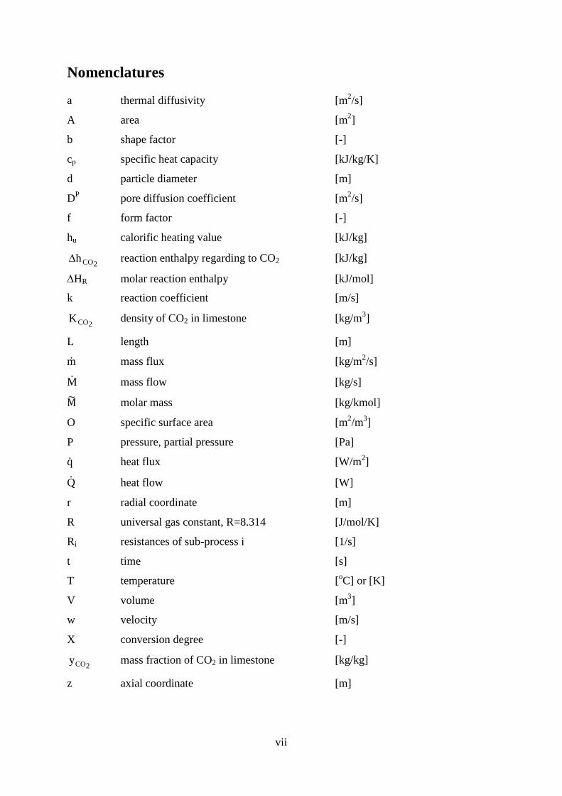
Nomenclatures a thermal diffusivity [m2/s]

A area [m2]

b shape factor [-]

cp specific heat capacity [kJ/kg/K]

d particle diameter [m]

DP pore diffusion coefficient [m2/s]

f form factor [-]

hu calorific heating value [kJ/kg]

2COh∆ reaction enthalpy regarding to CO2 [kJ/kg]

∆HR molar reaction enthalpy [kJ/mol]

k reaction coefficient [m/s]

2COK density of CO2 in limestone [kg/m3]

L length [m]

m mass flux [kg/m2/s]

M mass flow [kg/s]

M� molar mass [kg/kmol]

O specific surface area [m2/m3]

P pressure, partial pressure [Pa]

q heat flux [W/m2]

Q heat flow [W]

r radial coordinate [m]

R universal gas constant, R=8.314 [J/mol/K]

Ri resistances of sub-process i [1/s]

t time [s]

T temperature [oC] or [K]

V volume [m3]

w velocity [m/s]

X conversion degree [-]

2COy mass fraction of CO2 in limestone [kg/kg]

z axial coordinate [m]

viii

Greek symbols α heat transfer coefficient [W/m2/K]

β mass transfer coefficient [m/s]

γ air to lime ration [m3/kg]

δ thickness [m]

ε emissivity [-]

ζ empirical factor to determine porosity [-]

κ transient factor [-]

λ heat conduction coefficient [W/m/K]

µ dynamic viscosity [m2/s]

ρ density [kg/m3]

σ Stefan-Boltzmann constant, 5.67∙10-8 [W/m2/K4]

ν kinematic viscosity [m2/s]

ψ void fraction [-]

λ excess air number [-]

Subscripts a air

A area

ac lime cooling air

af combustion air

aL lance cooling air

aT transport air

D diffusion

E energy

eff effective

eq equilibrium

F front, core

F fuel

F furnace

fg flue gas

G gas

k reaction

ix

M mean

max maximum

min minimum

mix mixture

mono mono-dispersion

L length

L stoichiometric air demand

LS limestone

OX oxide

pd poly-dispersion

P pressure

P particle

S solid

S sphere

W wall, surface

Dimensionless number

Nu Nusselt number

Pr Prandtl number

Re Reynolds number

Sc Schmidt number

Sh Sherwood number

1

1 Introduction 1.1 Overview and motivation Lime is an important raw material, which is used in many branches of industry such as flue gas desulphurization, metallurgy, construction and manufacturing of paper. Lime is produced by thermal decomposition of limestone in shaft or rotary kilns. Lime manufacturers have been recently facing more restrictions. On the one hand, the fuel price, the main cost for lime production, has been increasing rapidly. On the other hand, the demand of reducing the emissions has become stricter. In addition, the quality of quicklime needs to be maintained. For lime manufacturers, it is very important that the following two parameters are achieved:

• Low energy consumption

• Desired (uniform) lime quality In fact, many lime manufacturers start to reduce their costs by using cheaper fuels, optimizing the burning system and atomizing the kiln process. However, mostly this is done by the method ‘learning by doing’, which consumes time and money. Burning lime or decomposition of limestone is an endothermic process, in which the kinetics of the burning process strongly depend on temperatures [1, 2]. In principle, to regulate or optimize the lime burning process, the temperature and the concentration (conversion) profiles in the kilns must be determined. However, with burning lime in shaft kilns, practical determinations of these parameters are very difficult. For example, the measurements of the kiln temperatures by using thermocouples face two main problems. Firstly, due to high temperature in the firing zone, common thermocouples (e.g., Ni-Cr/Ni) are often damaged; therefore, special thermocouples (e.g., Pt-Rh/Pt) are required. Secondly, due to the movements of solid bed with dust creation, thermocouples can also be damaged during measurements. In this case, simulations are an alternative way to model the temperature and the lime burning profiles. Many studies have been carried out to study the lime burning in shaft kilns. In most cases, however, the studies have been mainly concentrated on global energy and mass balances of the kilns [34-, 5 6 7 89]. Significant studies focusing on the temperature and the lime calcination profiles in the kilns are relatively rare. Numerical modeling of thermal processes in mixed-feed kilns was performed by Shagapov et al. [10] and YI-Zheng-ming et al. [11]. The basic kiln temperature and calcination profiles were simulated. No investigation of influencing factors, e.g., operating conditions, was performed. Senegacnik et al. [12,13] experimentally investigated temperature profiles and developed numerical solutions to calculate lime-burning

2

degree in an annular shaft kiln. The influence of convective heat transfer coefficient on the lime-burning degree was studied. With CFD (computational fluid dynamics) simulations, Drenhaus et al. [14] modeled the lime burning degree and the temperatures in a pilot vertical (normal) shaft kiln with 2 m bed height. The influence of the particle size on the time of lime calcination process was investigated. The results of the few researchers above are primary indications for basic understanding of the lime burning process in shaft kilns. However, for the purpose of process regulations and optimizations, further information needs to be explored because many parameters that affect significantly the lime burning process have not yet been investigated. Therefore, the aim of this dissertation is to develop comprehensive mathematical models to simulate the lime burning process in shaft kilns, focusing on normal shaft kilns and parallel flow regenerative (PFR) kilns. The models provide significant data required for designing and regulating shaft kilns. Furthermore, the models are also useful for a purpose of training the kiln personnel. To obtain experience within the operations is very time consuming since the kilns react to changes in operating parameters extremely slowly.

3

1.2 Lime production The world production of lime grew steadily from just under 60 million tons in 1960 to peaks of 120 million tons in 1995 and 170 million tons in 2006. Even due to the recent global economic recession (2008), published estimates of the world production of quicklime (Table 1-1) suggest that the total is approximately 310 million tons in 2010. Table 1-1 Estimations of world production of quicklime and hydrated lime, including dead-burned dolomite, 1995 – 2010, [15 16-17 1819].

Country 2000 2006 2010

Mt/year % Mt/year % Mt/year %

Brazil 5.7 4.9 6.0 3.5 7.7 2.5

China 21.5 18.5 75.0 43.5 190.0 61.3

Germany 7.6 6.6 7.0 4.1 6.8 2.2

India - - 4.0 2.3 14.0 4.5

Italy 3.5 3.0 5.2 3.0 2.8 0.9

Japan (quicklime only) 7.7 6.6 10.0 5.8 9.4 3.0

Mexico 6.5 5.6 4.0 2.3 5.7 1.8

Russia 8.0 6.9 8.0 4.7 7.4 2.4

United States 19.6 16.9 20.0 11.6 18.0 5.8

Other countries 35.9 30.9 32.8 19.1 48.2 15.5

Total 116.0 100 172.0 100 310.0 100

China, the United States and India are recently the top producers for lime, producing more than 200 million tons per year, or ~70 % of world output. They are followed by Brazil, Japan, Germany and Russia with about 10 % of world output. The principal industries using lime are the desulphurization of flue gas, steel processing, constructions and manufacturing of papers. As an example, Table 1-2 shows an estimation of using lime in EU in 2006.

Table 1-2 Estimations of using lime in EU, 2006, [20]. Industrial sectors Contribution, %

Steeling manufacturing 30 - 40

Environmental protection (e.g, flue gas desulfurization) 30

Construction and clay soil stabilization 15 – 20

Others: chemicals, PCC for paper, food and forestry, etc. 10 - 15

4

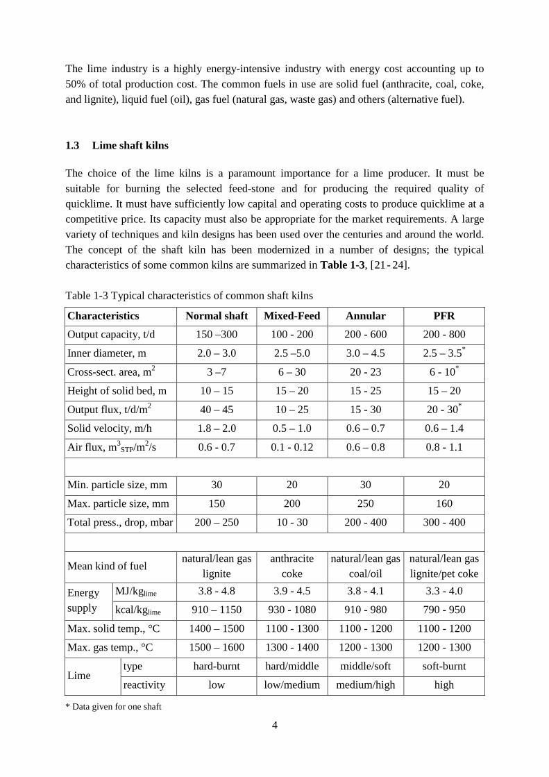
The lime industry is a highly energy-intensive industry with energy cost accounting up to 50% of total production cost. The common fuels in use are solid fuel (anthracite, coal, coke, and lignite), liquid fuel (oil), gas fuel (natural gas, waste gas) and others (alternative fuel). 1.3 Lime shaft kilns The choice of the lime kilns is a paramount importance for a lime producer. It must be suitable for burning the selected feed-stone and for producing the required quality of quicklime. It must have sufficiently low capital and operating costs to produce quicklime at a competitive price. Its capacity must also be appropriate for the market requirements. A large variety of techniques and kiln designs has been used over the centuries and around the world. The concept of the shaft kiln has been modernized in a number of designs; the typical characteristics of some common kilns are summarized in Table 1-3, [2122- 2324]. Table 1-3 Typical characteristics of common shaft kilns

Characteristics Normal shaft Mixed-Feed Annular PFR

Output capacity, t/d 150 –300 100 - 200 200 - 600 200 - 800

Inner diameter, m 2.0 – 3.0 2.5 –5.0 3.0 – 4.5 2.5 – 3.5*

Cross-sect. area, m2 3 –7 6 – 30 20 - 23 6 - 10*

Height of solid bed, m 10 – 15 15 – 20 15 - 25 15 – 20

Output flux, t/d/m2 40 – 45 10 – 25 15 - 30 20 - 30*

Solid velocity, m/h 1.8 – 2.0 0.5 – 1.0 0.6 – 0.7 0.6 – 1.4

Air flux, m3STP/m2/s 0.6 - 0.7 0.1 - 0.12 0.6 – 0.8 0.8 - 1.1

Min. particle size, mm 30 20 30 20

Max. particle size, mm 150 200 250 160

Total press., drop, mbar 200 – 250 10 - 30 200 - 400 300 - 400

Mean kind of fuel natural/lean gas

lignite anthracite

coke natural/lean gas

coal/oil natural/lean gas lignite/pet coke

Energy supply

MJ/kglime 3.8 - 4.8 3.9 - 4.5 3.8 - 4.1 3.3 - 4.0

kcal/kglime 910 – 1150 930 - 1080 910 - 980 790 - 950

Max. solid temp., °C 1400 – 1500 1100 - 1300 1100 - 1200 1100 - 1200

Max. gas temp., °C 1500 – 1600 1300 - 1400 1200 - 1300 1200 - 1300

Lime type hard-burnt hard/middle middle/soft soft-burnt

reactivity low low/medium medium/high high

* Data given for one shaft

5

Some designs are more suitable for low outputs (below 100 t/d), while others can be used for much higher outputs (up to 800 t/d). Normal acceptable size for the feed-stone ranges from a minimum of 20 mm to a top size of up to 200 mm and even up to 250 mm. Some kilns are suitable for operation on gaseous, liquid and solid fuels, while the options for others are more restricted. Nowadays, many lime producers operate two or more types of kilns, using different sizes of stone feed, and producing different qualities of lime. In practice, it typically takes about 1.75 kg of limestone to produce 1 kg of lime, the transportation of the raw material should be kept to a minimum. Therefore, lime kilns are normally located close to the limestone quarry. 1.4 Normal shaft kilns Figure 1-1 and Figure 1-2 illustrates the schemes of normal shaft kilns. These types of kilns are also named as RCE-kilns. In principle, the normal shaft kiln is a vertical single shaft where limestone is charged at the top of the kiln and quicklime is discharged at the bottom. The solid moves slowly downwards through the kiln by gravity. Heat to calcine the limestone is generated by fuel combustion where fuel is introduced with air in the middle of the kiln. Therefore, the solid above is preheated by hot exhaust gas in counter-current flow and the solid below is cooled by the cooling air introduced at the kiln bottom. In this way, material entering the kiln at the top is first preheated, then calcined and finally cooled during its passage through kiln. The gas leaving at the top of the kiln contains combustion gas and CO2 dissociated from the limestone. The kiln is theoretically divided into three operating zones. • Preheating zone: The upper part of the kiln where limestone is heated by hot exhaust gas

to its calcination temperature of about 810 - 840oC.

• Burning zone: The middle part of the kiln in which the limestone is decomposed into quicklime and CO2, fuel is burnt in preheated air.

• Cooling zone: The lower part of the kiln where lime emerging from burning zone is

cooled by air before discharge. 1.5 PFR shaft kilns The PFR kiln is a modern kiln with two-shafts (or three-shafts) defined by alternating burning and non-burning shaft operation. Figure 1-3 and Figure 1-4 show characteristic feature of a PFR kiln, which consists of two interconnected vertical shafts of either rectangular or circular cross sectional shape. Each shaft is subjected to two distinct modes of operation, burning and

6

non-burning mode. While one shaft operates in the burning mode (supplied by fuel and combustion air), the other shaft operates in the non-burning mode. In burning mode, one shaft is characterized by the parallel flow of combustion air/gases and stone, whereas, in non-burning mode the other shaft is characterized by the counter-current flow of off-gases and stone. Combustion air is introduced under pressure at the top of the preheating zone above the stone bed. The complete kiln system is pressurized. The combustion air is preheated by the stone prior to mixing with the fuel. The combustion gases exit the burning shaft through a crossover-channel into the non-burning shaft. The off-gases transfer heat to the stone during the non-burning mode and then the stone reclaims the heat to the combustion air during the burning mode. The above method of operation incorporates two key concepts:

• The stone-packed in the preheating zone in each shaft acts as a regenerative heat

exchanger. The surplus heat in the gases is transferred to the stone in the non-burning mode. It is then transferred from the stone to the combustion air in the burning mode. Because of this alternative heat transfer, PFR kilns have the lowest specific energy consumption compared with other types of kilns.

• In parallel flow of PFR kilns, the fuel is introduced at the upper end of the burning zone

and the combustion gases travel parallel to the material. As a result, the heat released from fuel combustion is mostly absorbed by the solid for calcination of limestone so that the temperature in the burning zone is typically 900 – 1200 °C on average. Because of parallel flow heating, PFR kilns are suitable for the production of soft-burnt, highly reactive lime.

Depending on the kiln manufacturers, different concepts of optimizing the kiln process have been developed to design the PFR kilns. For example, the shapes of the cross-section can be round / circular, rectangular or special design with D-shape (Cimpprogetti kilns, Figure 1-4); the cross-over channel can be direct (for rectangular kilns) or indirect / circular (for circular kilns). Some different designs of the kilns can be seen from Figure 1-5 to Figure 1-6.

7

Figure 1-1: Schematic diagram of normal shaft kilns Figure 1-2: Normal shaft kiln (source: http://www.rhi.at)

lime

coo

ling

bur

ning

preh

eatin

g z=0

z=L

limestone

air

fuel & air

gas

burners

burning zone

cooling zone

preheating zone

8

Figure 1-3: Schematic diagram of a PFR shaft kiln Figure 1-4: PFR shaft kiln (source: http:// www.cimprogetti.com)

limestone gas

lime air

fuel

reversal

z=0

z=L

preh

eatin

g

burn

ing

cool

ing

bu

rnin

g sh

aft

no

n-bu

rnin

g sh

aft

bu

rnin

g sh

aft

no

n-bu

rnin

g sh

aft

air

limestone

lime

air gas

http://www.cimprogetti.com/

9

Figure 1-5: Circular PFR kiln (source: http:// www.maerz.com) Figure 1-6: Rectangular PFR kiln (source: http:// www.maerz.com)

lances

direct channel

burning

cooling

lances

burning

circular channel

cooling

http://www.maerz.com/


10

Figure 1-7: PFR- kiln (source: http:// www.maerz.com)

Figure 1-8: PFR- kiln (source: http:// www.cimprogetti.com)


http://www.cimprogetti.com/

11

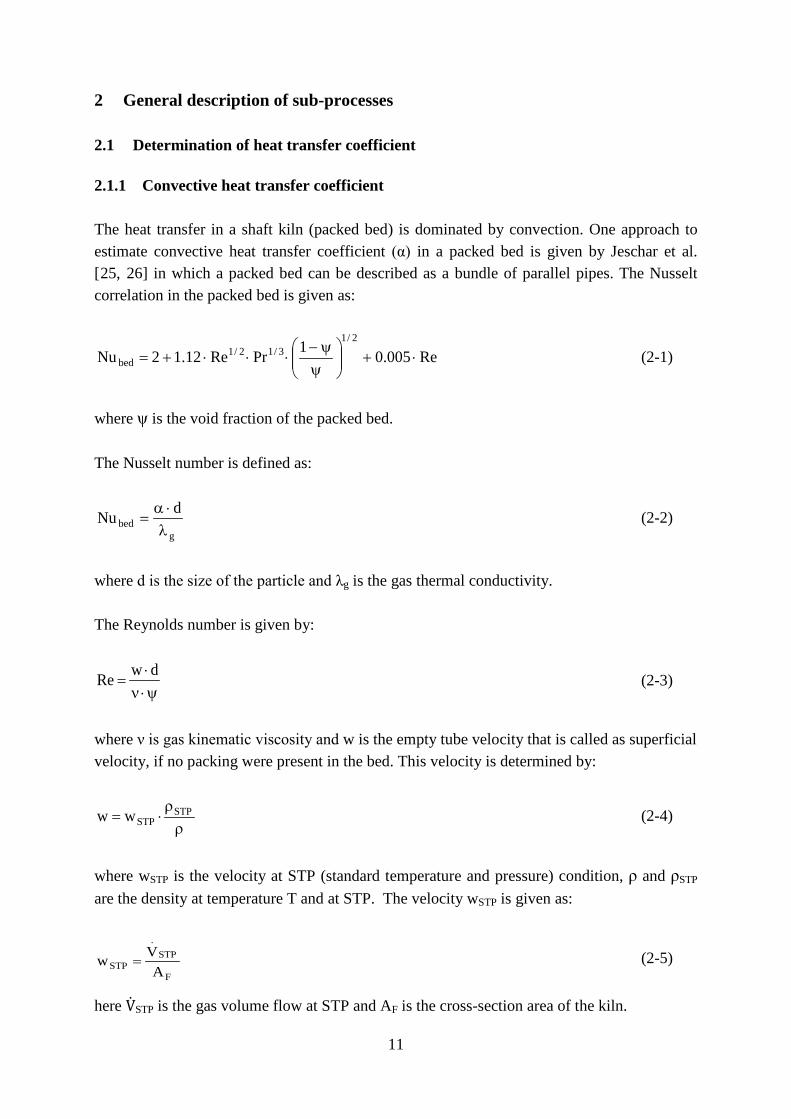
2 General description of sub-processes 2.1 Determination of heat transfer coefficient 2.1.1 Convective heat transfer coefficient The heat transfer in a shaft kiln (packed bed) is dominated by convection. One approach to estimate convective heat transfer coefficient (α) in a packed bed is given by Jeschar et al. [25, 26] in which a packed bed can be described as a bundle of parallel pipes. The Nusselt correlation in the packed bed is given as:

Re005.01PrRe12.12Nu2/1

3/12/1bed ⋅+

ψψ−

⋅⋅⋅+= (2-1)

where ψ is the void fraction of the packed bed. The Nusselt number is defined as:

gbed

dNuλ⋅α

= (2-2)

where d is the size of the particle and λg is the gas thermal conductivity. The Reynolds number is given by:

ψ⋅ν⋅

=dwRe (2-3)

where ν is gas kinematic viscosity and w is the empty tube velocity that is called as superficial velocity, if no packing were present in the bed. This velocity is determined by:

ρρ⋅= STP

STPww (2-4)

where wSTP is the velocity at STP (standard temperature and pressure) condition, ρ and ρSTP are the density at temperature T and at STP. The velocity wSTP is given as:

F

STP.

STP AVw = (2-5)

here VSTP is the gas volume flow at STP and AF is the cross-section area of the kiln.

12

The Prandtl number is defined as:

g

pcPr

λ

⋅ρ⋅ν= (2-6)

here cp is the specific heat capacity of the gas. There is another model so called single-particle model, which is also commonly used to determine the heat transfer coefficient in a packed bed. Bes [27] has compared the convective heat transfer coefficients obtained from the two approaches. The results from the model based on single particle are slightly lower than those from the hydraulic diameter model. For the typical air velocity of about 1 m/s at standard temperature and pressure, the difference between the results of both approaches is less than 20%. 2.1.2 Overall heat transfer coefficient The solid particle has a temperature distribution in a radial direction since the heating-up and the cooling-down of solid particles is a transient process. To calculate the temperature profile inside the particle, the Fourier differential equation must be solved and this requires a lot of effort. In the industrial practice, however, an assumed homogeneous average temperature (calorific temperature) is often more preferred, to make the energy balance easier. For this purpose, Jeschar et al. [26] & Mills [28] introduced a modified overall heat transfer coefficient, ακ.

λ⋅κ+

α

=ακ 2/d11 (2-7)

where λ is the thermal conductivity of the solid particle, and κ is the transient factor given as:

=κ

sphereafor5cylinderafor4plateafor3

(2-8)

2.2 Determination of mass transfer coefficient In simulation of limestone decomposition, the convective mass transfer of the produced CO2 into the gaseous ambience must be calculated. With analogy to heat transfer, the mass transfer

13

coefficient of CO2 from the limestone surface to the gas, β, can be calculated from the Sherwood function.

Re005.01ScRe12.12Sh2/1

3/12/1 ⋅+

ψψ−

⋅⋅⋅+= (2-9)

The Sherwood function is defined as:

Air2CODdSh−

⋅β=

(2-10) where DCO2-Air is the binary diffusivity of CO2 in air, which will be determined in the next. The Schmidt number Sc is defined as:

Air2CODSc

−

ν=

(2-11)

2.3 Gas mixture properties To calculate the Nusselt and the Reynolds numbers the material property values have to be calculated at the gas temperature T because the temperature difference is significant. The material property values are calculated with the following equations given by Specht [29]:

λ

⋅λ=λ

n

oo T

T (2-12)

µ

⋅µ=µ

n

oo T

T (2-13)

cn1n

oo T

Taa−+µ

⋅= (2-14)

1

oo T

T−

⋅ρ=ρ (2-15)

14

cn

opop T

Tcc

⋅= (2-16)

1n

oo T

T+µ

⋅ν=ν

(2-17)

1Dn

oo T

TDD+

⋅=

(2-18)

From Eq.(2-18), the diffusivity of the CO2 in air, DCO2-Air given before in Eqs.(2-10)-(2-11), can be approximated with Do= 0.14∙10-4 m2/s and nD=1.71. In the above equations, To is the reference temperature taken as 273 K. The material properties of gas components at the temperature To are gathered in Table 2-1. Table 2-1 Material properties of gases at To = 273 K

Gas 𝑀� ρo cpo nc

λo nλ μo nμ Pr

unit kg/kmol kg/m3 J/kg/K - W/m/K - mg/m/s - - N2 28 1.26 1000 0.11 0.024 0.76 16.8 0.67 0.70 CO 28 1.26 1000 0.12 0.024 0.78 16.8 0.67 0.70 Air 29 1.29 1000 0.10 0.025 0.76 17.4 0.67 0.70 O2 32 1.44 900 0.15 0.025 0.80 19.7 0.67 0.70

CO2 44 1.98 840 0.30 0.017 1.04 14.4 0.77 0.73 H2O 18 0.81 1750 0.20 0.016 1.42 8.7 1.13 0.95

The properties of gas mixtures can be calculated with the following formulas:

∑ ⋅ρ=ρ iiM x~ (2-19)

∑ ⋅λ≈λ iiM x~ (2-20)

∑ ∑ ρ⋅⋅ρ

=⋅= iipiM

ipipM x~c1xcc

(2-21)

where xı� is the molar or volume fraction of component i in a gas mixture and xi the mass fraction of component i in a gas mixture.

15

2.4 Flow pattern in packed bed 2.4.1 Void fraction

Shaft kilns are basically packed bed reactors. The void fraction has significant effect on the heat and mass transfer. The void fraction Ψ of a packed bed is defined as:

volumeBedvolumePackingvolumeBed −

=Ψ

(2-22)

The void fraction can be influenced by the method of packing (random or regular, loose or dense), particle shape (sphere, cylinder, etc), and particle size distribution. For infinitely extended, regular packing of equally sized, large spheres the void fraction is:

0.476 for simple cubic packing 0.395 for cubic space centered packing 0.259 for cubic face centered packing.

For random packing of equally sized, large spheres the void fraction is:

0.4 - 0.42 for loose packing 0.36 - 0.38 for dense packing. Figure 2-1 shows a particle size distribution in a packed bed as an example. The void fraction does not depend on the average particle size, but much on the width of the particle size distribution, which is characterized by the ratio between the maximum (coarse, dc) and minimum (fines, df) size, Furnas [30]. Figure 2-2 shows the influences of the ratio dc/df and the volume fraction (Qf) of fine particles on the void fraction. When the ratio dc/df =1 (mono-dispersion), the void fraction has the maximum value (Ψmono) of about 0.4. The void fraction decreases rapidly with the increases of the ratio dc/df, especially with dc/df greater than 3. The theoretical minimum value of the void fraction is about 0.16. In addition, at the same ratio dc/df, the void fraction decreases with increasing the Qf from 0 to about 30 %, but it increases while Qf is greater than 30 %. There are two limiting cases in which the void fraction depends on the Ψmono and the Qf as given in the figure. The more closely or sharply the particle size distributes, the lower is the void fraction. An empirical equation to determine the actual void fraction of a packed bed with a random packing of particles with different sizes, is introduced by Tsotsas [31]:

16

[ ]32monopd 112.0017.0259.01 ζ−ζ+ζ−Ψ=Ψ (2-23)

where Ψpd stands for the void fraction of poly-dispersion packing of a packed bed and ζ is a corresponding factor defined as:

( )

−=ζ

∑∑ 1

d/V

d/V2

ii

2ii (2-24)

where Vi and di are the volume fraction and the size of fraction i.

Figure 2-1: An example of particle size distribution of limestones

02468

101214161820

115

110

105

100 95 90 85 80 75 70 65 60 55 50 45 40 35 30 25 20 15

Mas

s fra

ctio

n in

%

Particle size in mm

17

Figure 2-2: Bed porosity of bi-dispersed packing of spheres, Furnas [30]

Two limiting cases:

( )

−

⋅ΨΨ−

−⋅Ψ=Ψf

f

mono

monomono1 Q1

Q11 and

⋅Ψ+Ψ−

⋅Ψ=Ψfmonomono

fmono2 Q1

Q

Figure 2-3: Radial porosity profile in tubes packed with imperfect spheres

0,16

0,2

0,24

0,28

0,32

0,36

0,4

0 0,2 0,4 0,6 0,8 1

Void

frac

tion Ψ

bed

Volume fraction of fines, Qf

dc/df=2

3

5

20

10 Ψ1 Ψ2

Ψmono

c: coarse f: fine

Ψmin=Ψ2mono

18

The void fraction mentioned above is an average void fraction of the entire packed bed. However, in a radial direction of the packed bed, especially in the region near the wall, the void fraction is much higher than the others Giese [32]. This is due to the wall effect as shown in Figure 2-3.

2.4.2 Pressure drop The pressure drop in the packed bed can be described by two different models: a) a hydraulic diameter model and b) a one particle cross-flow model, Bes [27]. In this study, the hydraulic diameter model is used to calculate the pressure drop. In this model, the flow through a packed bed can be regarded as fluid flow past some number of submerged objects, in which the hydraulic diameter is defined as:

OAVd

H

HH

ψ== (2-25)

where VH is the volume that is available for flow in the packed bed, AH is the wetted surface in the packed bed and O is the specific surface are of the packed bed, which are determined from the specific surface (AP) and the volume (VP) of a single particle in the bed:

( )ψ−⋅= 1AV

OP

P (2-26)

The specific surface area O can be calculated if the geometry of the particles and the void fraction in the bed are known. For examples, with spheres, the value of O is obtained as:

( )ψ−⋅= 1d6O (2-27)

There are two existing equations given Ergun [33] and Brauer [34] to determine the pressure drop of a packed bed. As an example, the Ergun equation is used in this dissertation to determine the pressure drop. This equation is based on the model conception that the real packed bed can be replaced by a parallel connection of flow channels, and the pressure drop calculation is similar to the one phase pipe flow, however with the hydraulic diameter of the packed bed as characteristic dimension. The Ergun equation is described as follows:

( ) ( ) dzdw.1.75.1dz

dw1150P

L

0z

2

3

L

0z23

2

∫∫==

⋅ρΨΨ−

+⋅ν⋅ρ

⋅ΨΨ−

⋅=∆ (2-28)

where d� is the Sauter mean diameter and w is the superficial velocity defined as before.

19

The first term of the Ergun equation describes the change of pressure under viscous flow, while the second term accounts for change of pressure at turbulent flow (kinematic energy loss). The second term is dominant in this equation. It can be seen from this equation that the pressure drop along the length of the packed bed depends on the packing size, the bed void fraction, the gas velocity, density and viscosity. The Sauter mean diameter is described as:

1

i

in

1i d1

VV

d−

=

⋅= Σ

(2-29)

where V is total mass or volume of all solid particles and Vi is mass or volume of solid particle class i. In the Eq. (2-28), the void fraction and the particle size are constant values, however the gas properties (viscosity, density and velocity) are functions of gas temperature. Therefore, to determine the pressure drop the gas temperature must be calculated. The method of calculating the gas temperature will be mentioned in one of the following chapters, which described process modeling and simulation.

20

3 Decomposition of limestone 3.1 Limestone characterization The main component of limestone is calcium carbonate (CaCO3), which is formed by the compaction of the remains of coral animals and plants on the bottoms of oceans. It can be a soft white substance (chalk) through to a very hard substance (marble). Most commercial limestone deposits are a brownish rock. As an example, the chemical composition and bulk density of some limestone are shown in Table 3-1, Cheng [35]. Table 3-1 Chemical composition and bulk density of some typical limestone

Chemical composition, (%)

Cretaceous limestone

Jurassic limestone

Devonian limestone

Marble

CaO 52.47 55.70 54.29 55.34

MgO 0.30 0.190 0.39 0.59

SiO2 4.68 0.240 1.83 0.08

Fe2O3 0.24 0.032 0.21 0.05

Al2O3 0.63 0.043 0.08 0.01

K2O 0.08 0.007 0.02 0.004

Na2O 0.03 0.013 0.01 0.01

BaO 0.01 0.012 0.02 0.01

SrO 0.03 0.004 0.02 0.01

MnXOY 0.03 0.013 0.02 0.004

SO3 0.05 - 0 - Weight loss (CO2), %

41.50 43.51 43.05 43.97

Density, (kg/m-3) 2510 2610 2680 2710 3.2 Lime quality 3.2.1 Lime reactivity The burning grade of lime can be characterized by its reactivity. The lower the decomposition temperature is held during the decomposition of limestone, the higher will be the lime reactivity. In the practice, the lime reactivity is detected by the velocity of temperature increase of the water-lime-slurry, after the 150 g lime powder of grain size of 0-3 mm was dosed into 600 ml distilled water of 20°C. From the slaking-curve, which indicates the temperature increase of the slurry due to the hydration reaction of lime, a parameter t60 can be read out, which means after this time the slurry temperature will increase from 20 up to 60°C

21

(DIN EN 459-2 2002). When t60 is shorter than 2 min, then the lime is said to be soft-burnt. When t60 is in the range 2 min to 6 min, the lime is said as medium-burnt and the lime is hard-burnt when t60 is longer than 6 min. As an example, Figure 3-1 shows the results of measuring t60 of three different limes, Schwertmann [36]. In this figure, it can be seen that the t60 of a soft-burnt lime sample is about 1.8 min, t60 of a medium-burnt sample is 4 min and that of a hard-burnt lime is approximately 7 min.

Figure 3-1: Measurement of lime reactivity, Schwertmann [36]

Figure 3-2: SEM pictures of lime, Schwertmann [36]

20

25

30

35

40

45

50

55

60

65

70

75

0 2 4 6 8 10 12 14 16 18 20

Tem

pera

ture

in o C

time in min

Soft-burntMiddle-burntHard-burnt

Tmax

t60

Soft-burnt Middle-burnt Hard-burnt

22

The t60-value is correlated with the specific surface area of the lime (for example BET-surface area), or the porosity of the lime. The higher the temperature at the end of the burning process, the smaller will be the specific surface and the porosity; hence the t60-value will be longer. This is decided by the development of the crystal structure or the sintering effect in the lime. Under Scanning Electronic Microscope (SEM), limes of different reactivity have different crystal structure and pores system, which is shown in Figure 3-2. 3.2.2 Residual CO2 in lime Another measurement of the lime quality is the residual CO2 (Res.CO2) in the lime. This refers to the content in percentage of the mass of the un-reacted CO2 to the mass of the lime.

)R(2CO.

LS.

)R(2CO.

2CO.

2

MM

MMCO.sRe−

−= (3-1)

where MCO2 is the total mass flow of CO2 in limestone, MCO2(R) is the total mass flow of CO2 decomposed and MLS is the mass flow of limestone, which is related to MCO2 as:

2CO.

2COLS

.M

y1M ⋅= (3-2)

where yCO2 is the mass fraction of CO2 in the limestone, which varies for different limestones, for example, with pure calcium carbonate 2COy =0.44 kgCO2/kgLS.

The conversion degree X is defined as the ratio of the total mass of reacted CO2 to the mass of CO2 content in the limestone

2CO.

)R(2CO.

M

MX = (3-3)

From above equations the relation between the conversion degree and the residual CO2 content is obtained as:

2CO2

22CO

y)CO.sRe1(CO.sRey

X⋅−

−= (3-4)

and

1Xy

11

Xy

11CO.sRe

2CO2CO

2−

⋅

−−

= (3-5)

23

3.3 Limestone decomposition model The decomposition of limestone is an endothermic topochemical reaction described as follows, Oates [1]: CaCO3 + ΔHR = CaO + CO2 (3-6) (solid) (reaction enthalpy) (solid) (gaseous) The calcination process can be explained by using a partially decomposed piece of carbonate, whose profiles of CO2 partial pressure and temperature are shown in Figure 3-3. The specimen comprises a dense carbonate core surrounded by a porous oxide layer. In the calcination reactor at temperature Tg heat is transferred by radiation and convection (symbolized by α) to the solid surface at a temperature of Tsw. By means of thermal conduction (λ) heat penetrates through the porous oxide layer to reach the reaction front, where the temperature is Tsf. As the reaction enthalpy is many times greater than the internal energy, the heat flowing further into the core is negligible during reaction. Therefore, the core temperature is only slightly lower than the front temperature. Once heat is supplied, the chemical reaction (k) then takes place, for which the driving force is the deviation of CO2 partial pressure from the equilibrium (Peq- Pf). The released CO2 diffuses (DP) through the porous oxide layer to the surface and finally passes by convection (β) to the surroundings where the CO2 partial pressure Pg exists. The four physical transport processes and the chemical kinetics involved are therefore interconnected.

Figure 3-3: Decomposition model of limestone particle

Pg

CaO

CaCO3

Pf

Tsw

Pw

Peq

rf rw

Tg

α λ

𝐷𝑝

k

β

P

T Tsf

Q .

Mco2.Δh

24

To calculate the decomposition of a single limestone particle, a one-dimensional shrinking core model was established by Szekely et al. [37] and Kainer et al. [38], which is based on the assumptions of an ideal sample geometry (sphere, cylinder or plate), a pseudo steady state condition and constant material properties. A system of heat and mass balance equations, which are used to calculate the decomposition of limestone, are given as follows: The heat balance equation (e.g., for spheres) is obtained by heat conduction from the particle surface through the lime layer to the reaction front.

( )sfswfw

fw

.-TT

)rr(rr4Q ⋅

−λ

⋅π= (3-7)

The mass balance equation of CO2 is obtained by combining the mass transfer at the particle surface and the diffusion in the lime layer:

−⋅⋅

β

+−

⋅π=sw

g

sf

f

2COP

fw

P

fw2CO.

TP

TP

R1

1D

rrDrr4M (3-8)

For the reaction at the front, the reaction rate is proportional to the deviation of partial pressure from equilibrium.

( )feqsf2CO

2f2CO

.PP

TRkr4M −⋅⋅

⋅π= (3-9)

where the equilibrium pressure is defined as:

∆−⋅=

sf

Roeq RT

HexpPP (3-10)

with Po is 2.15x107 bar and ΔHR is 168 kJ mol-1, Silva et al. [39]. The heat flow and the mass flow of the CO2 are finally related by:

2CO.

2CO

.MhQ ⋅∆= (3-11)

where ΔhCO2 is the specific reaction enthalpy corresponding to the produced CO2 in mass, 3820 kJ/kg.

25

From above equations, the decomposition parameters such as mass flows of CO2 decomposed (MCO2), moving reaction front (rf) and reaction temperature (Tsf), can be calculated. The mass flow of CO2 can be expressed as:

dtdrKr4M f

2CO2f2CO

.⋅⋅π−= (3-12)

where KCO2 is the density of CO2 in the limestone, e.g. 1190 kgCO2/m3 for a pure limestone with a density of about 2700 kg/m3. It is more convenient to introduce the conversion degree X for calculations. The conversion degree X is given before in Eq.(3-3). It can be defined in another way related to the moving front with time dependency as:

b

w

f

)0t(2CO.

)t(2CO.

)0t(2CO.

rr1

M

MMX

−=

−=

=

= (3-13)

where b is the shape factor, b=1, 2 or 3 for a plate, cylinder or sphere, respectively. From Eq. (3-7) to Eq.(3-13), a couple of differential equations were derived to calculate the conversion degree X and the decomposition temperature Tsf , Kainer et al. [38].

( )[ ] 1XfRdtdX

1 =⋅⋅ λ (3-14)

( ) ( )[ ] 1XfRXfRRdtdX

2k1D =⋅+⋅+⋅ β (3-15)

where f1(X) and f2(X) are the form functions, for example with spheres, these functions are described as:

( ) ( )

−−⋅= − 1X12Xf 31

1 (3-16)

( ) ( ) 32

2 X131Xf −−⋅= (3-17)

The resistances Ri, where Tsf is included, are given in the following equations.

26

b2r

TThK

R2

w

sfsw

2CO2CO

⋅λ⋅⋅

−

∆⋅=λ (3-18)

kr

PPTRK

R w

geq

sf2CO2COk ⋅

−

⋅⋅= (3-19)

bD2r

PPTRK

R P

2w

geq

sf2CO2COD ⋅⋅

⋅−

⋅⋅= (3-20)

br

PPTRK

R w

geq

sf2CO2CO

⋅β⋅

−

⋅⋅=β (3-21)

3.4 Determination of material properties The material properties of limestones such as the thermal conductivity, the reaction coefficient and the pore diffusivity are important input parameters for modeling the lime burning process. Therefore, in this study, experiments were carried out to determine these parameters. The experimental apparatus is shown schematically in Figure 3-4. According to Kainer et al. [38], the material properties can be evaluated by an analytical solution. The evaluation requires particles of cylindrical or spherical shape. Hence, cylinders were prepared from large stone pieces using hollow drillers. In Figure 3-4, the limestone specimens were suspended from a balance with which the weight loss and therefore the conversion degree could be recorded continuously. In order to have well-defined flow conditions around the specimen, pure air was introduced from the bottom of the furnace with a known volume flow. A small hole was drilled in the center of the specimen. The temperature in the hole was measured simultaneously with the weight loss by a thermocouple. The knowledge of this core temperature is essential to analyze the material properties of limestone. The tests were performed using cylinders with diameters in the range of 20 – 25 mm, Figure 3-5. The length / diameter ratios of cylinders ranged from 4 to 10 and the cylinders were insulated at the top and bottom so that they could be regarded as infinitely long and treated as one-dimensional.

27

Figure 3-4: Experimental apparatus for measuring limestone decomposition

Figure 3-5: Cylindrical samples of limestones from different sources

1 chamber furnace 2 carbonate sample 3 balance 4 pump CO2 feed-in 5 CO2 flow meter 6 pump air feed-in 7 air flow meter 8 ceramic packed bed 9 thermocouple for gas temp 10 thermocouple for gas temp 11 thermocouple for sample temp. 12 measured data logger

3 12

2

1

8

CO2 Air

4 5 6 7

9

10

11

28

Figure 3-6: Conversion degree and calcination temperature of limestone of different origins

As an example, Figure 3-6 shows the results of measuring the conversion degree and the core temperature for three different kinds of limestones from Germany. Experiments were carried out at the same furnace temperature of 1000 °C. It can be seen that the limestone Ge. 1 decomposes completely after 45 min while the limestone Ge. 3 needs a significant longer time with about 65 min. The limestone Ge. 2 is in between the two other samples. The calcination temperatures are also different. The limestone Ge. 2 has the lowest core temperature with about 860 oC and the limestone Ge. 3 has the highest core temperature with about 890 oC. The material properties of three above limestones are determined by using an analytical solution given by Kainer et al. [38] and the results are shown in Table 3-2. It can be seen that the material properties are significantly different, especially the reaction coefficient and the pore diffusivity. The difference in the material properties causes the difference in the decomposition behavior.

0

0,2

0,4

0,6

0,8

1

0 20 40 60 80

Con

vers

ion

degr

ee

1 2

3

Ge. 1 Ge. 2 Ge. 3

a)

700

750

800

850

900

950

1000

0 20 40 60 80

Cor

e te

mp.

, in

oC

Time in min

1

2

3

Ge. 1 Ge. 2 Ge. 3

Tg=1000oC d=25 mm

b)

29

Table 3-2 Properties of limestone of different origins Limestone k∙10-2, [m/s] λ [W/m/K] DP∙10-4 [m2/s]

Ge.1 0.98 0.70 1.63 Ge.2 0.76 0.74 1.28 Ge.3 0.54 0.73 2.4

30

4 Energy and mass balance 4.1 Energy and mass balance of normal shaft kiln 4.1.1 Process description The schematic diagram of the normal shaft kiln is shown before in the Figure 1-1 with three operating sections: the preheating, the reaction and the cooling zones. To calculate the energy consumption, the reaction and the cooling zone have to be treated together and the preheating zone has to be separated, Bes [40]. This division is necessary because the gas temperature (Tg) between the preheating and the reaction zone has to be higher than the solid equilibrium temperature (Teq) at that position so that the 2nd law of the thermodynamics is fulfilled, as shown in Error! Reference source not found.. This equilibrium position is called as ‘pinch’ point in chemical engineering. The balance is independent on the direction of the gas flow in the reaction zone. In case of the counter-current flow, the gas leaving the reaction zone has the highest CO2 concentration at the transition to the preheating zone. Therefore, this CO2 concentration determines the end of the preheating and the beginning of the reaction.

Figure 4-1: Principal temperature profiles in normal shaft kilns

4.1.2 Energy balance Error! Reference source not found. shows the heat input and output flows in the reaction zone and the cooling zone. In these zones, the main heat input is the mass of fuel Mf multiplied by

Tem

pera

ture

Teq

fuel / secondary air

Axial position

Tsolid

Tair

Tgas

preheating cooling reaction

Tsolid

Tg

Tg.mix

stone air

31

its heating value hu. The other heat inputs are from the limestone at equilibrium temperature Teq and from the air. The heat from the limestone is MLS·cLS·Teq. The air flow is divided into the air flow through the cooling zone Mac and the air flow blown into the kiln with the fuel Maf. The air blown in with the fuel can be preheated (except transport air). Therefore, its temperature was denoted as Taf. The heat input for these two air flows Ma·cpa·Ta is calculated relative to the ambient temperature Te (Ta=Te).

Figure 4-2: Heat inputs and outputs in the reaction and cooling zones of normal shaft kilns The main energy output is the energy consumed by the limestone decomposition ML·ΔhL·XL. Here, XL is the conversion degree and Lh∆ = 3.18 MJ/kglime is the reaction enthalpy related to the ambient temperature. Experimental research results summarized by Chai and Navrotsky [41] mentioned the value h~∆ =178 ± 1 MJ/kmol. The other heat outputs are the heat output with the lime, the gas and the heat loss through the wall. The change of the flue gas and the lime mass flows due to the incomplete calcination can be neglected with an error smaller than 1%. The decomposition of the magnesite fraction is assumed to be equal to the limestone decomposition for simplifying and the evaporation enthalpy of the moisture in the limestone is neglected. In heat balances, the enthalpies are always referred to the reference temperature Tref. (0 oC), Bes [40]. The sensible heat of the phase is given as:

TcM)C0T(cM)TT(cMQ po

p.refp

.⋅⋅=−⋅⋅=−⋅⋅=

(4-1)

Here the temperature T is taken in degree Celsius.

reaction and cooling preheating

limestone

flue gas

32

The energy balance equation is given as:

wgpggLLLLdLL

eqLSLSafpaafepaacuf

QTcMXhMTcM

TcMTcMTcMhM

+⋅⋅+⋅∆⋅+⋅⋅=

⋅⋅+⋅⋅+⋅⋅+⋅

(4-2)

The air mass flow depends on the air demand L, the kind of fuel, the air excess number λf and the operating conditions:

ffafaca MLMMM ⋅⋅λ=+= (4-3) The mass flow of limestone LSM is given by:

2COLLS y1

1MM−

⋅= (4-4)

The flue gas mass flow gM consists of the air flow, the fuel flow and the CO2 flow produced

by the calcination L2COM :

L2COfag MMMM ++= (4-5)

where the CO2 flow produced by decomposition is given by:

L2CO

2CO2COLSL2CO M

y1y

yMM ⋅−

=⋅= (4-6)

From Eq. (4-2) - (4-6) the energy consumption per kg of lime is obtained.

( ) ugpgfepaf

L

weqLS

2COgpg

2CO

2COLLLdL

L

uf

h/]TcL1TcL[1MQTc

y11Tc

y1y

XhTc

MhME

⋅⋅⋅λ+−⋅⋅⋅λ+

+⋅⋅−

−⋅⋅−

+⋅∆+⋅

=⋅

=

(4-7)

There are different kinds of fuels commonly used in shaft kilns such as natural gas, lean gas, oil, lignite, anthracite and coal. For example, the composition, the air demand and the net heating values, for three types of fuel: natural gas, lignite and anthracite are shown in Table 4-1 and Table 4-2. Table 4-1 Composition in %Vol, air demand and net heating value of natural gas

CH4 C2H6 H2 CO2 CO N2 L

[kgair/kgfuel] hu

[MJ/kgfuel] Natural gas

0.93 0.05 0 0.01 0 0.01 16.1 47.7

33

Table 4-2 Composition (dry and ash free), air demand and net heating value of solid fuel

C H O S N Water Ash L

[kgair/kgfuel] hu

[MJ/kgfuel] Anthracite 0.92 0.04 0.02 0.01 0.01 0.04 0.06 10.1 29.7 Lignite 0.70 0.05 0.25 - - 0.10 0.06 6,8 20 To solve the Eq. (4-7) it is necessary to know the value of the equilibrium temperature Teq, which has to be lower than the gas temperature Tg. Both temperatures are unknown. The equilibrium temperature depends on the carbon dioxide concentration and thus on the kind of fuel and the operating conditions. This dependence will be described in the following chapter. 4.1.3 Mass balance of CO2 The carbon dioxide concentration in the flue gas decides the equilibrium temperature Teq at which the decomposition starts. The CO2 in the flue gas is produced by both the combustion of the fuel and the decomposition of the limestone. The carbon dioxide concentration in the flue gas leaving the reaction zone fg2COx can be calculated from the mass balance of CO2:

fg2COL2COgfL2COf2COgf x)MM(MxM ⋅+=+⋅ (4-8)

The mass flow of CO2 produced by the fuel combustion f2COgf.

xM ⋅ and the mass flow of

CO2 produced by the limestone decomposition L2CO.

M leave the reaction zone with total gas flow:

L2COgfg MMM += (4-9)

The mass flow of combustion gas depends on the mass flow of the fuel and the air as:

( ) fffagf ML1MMM ⋅⋅λ+=+= (4-10)

The CO2 concentration f2COx in the combustion gas is determined according to Specht [42].

The CO2 flow produced by decomposition is given by:

L2CO

2CO2COLSL2CO M

y1y

yMM ⋅−

=⋅= (4-11)

The lime mass flow ML can be replaced by the energy consumption E.

34

L

uf

MhME

⋅=

(4-12)

Then the CO2 concentration of the flue gas leaving the reaction zone is calculated as:

( )

( ) u2CO

2COf

u2CO

2CO)f(f2COf

fg2CO

hy1

yL1E

hy1

yxL1E

x⋅

−+⋅λ+⋅

⋅−

+⋅⋅λ+⋅

=λ

(4-13)

From Eq. (4-13), it can be seen that the CO2 fraction in the flue gas depends on the energy consumption E, the air excess number λf, the type of limestone 2COy and the kind of fuel hu.

4.1.4 Equilibrium temperature

As mentioned above, to solve the energy balance equation, Eq. (4-7), it is necessary to know the equilibrium temperature Teq at which the decomposition begins. This temperature is a function of the CO2 concentration fg2COx or the CO2 partial pressure in the flue gas PCO2. The

equilibrium temperature Teq is obtained from the Eq.(3-10) in the chapter 3 as:

1

2CO

oReq P

PlnRHT

−

⋅

∆= (4-14)

where the CO2 partial pressure PCO2, which depends on the CO2 concentration and the kiln pressure Pkiln, is calculated as:

lnkifg2CO2CO PxP ⋅= (4-15)

From Eq. (4-13) to Eq. (4-15), it can be seen that the equilibrium temperature also depends on the energy consumption, the air excess number, the type of limestone and the kind of fuel. As an example, Figure 4-3 and Figure 4-4 show the CO2 concentrations and calcination temperatures for natural gas and lignite fuel as functions of the excess air number. The energy consumptions of E = 3.8 MJ/kglime and E = 4.5 MJ/kglime which correspond to a relatively low and high energy usage were taken. The lower the energy consumption and the air excess number, the higher is the carbon dioxide concentration. Lignite gives the higher CO2 in the flue gas. The line for E = 3.8 MJ/kglime for lignite ends at λf = 1.05, since for the higher excess

35

air numbers, such so low energy consumption is no more possible. Similarly the line for E = 3.8 MJ/kglime for natural gas ends at λf = 1.3. 4.1.5 Energy consumption With the set of equations given previously, the energy consumption can be calculated iteratively. In Eq. (4-7) all values are known except the gas temperature Tg between the preheating and the reaction zone. This temperature depends on the heat exchange, the zone length and the lime throughput and thus on the kinetic of the process. The larger the heat transfer and the higher the kiln, the smaller is the difference in temperature between gas and solid. Because the gas temperature Tg is unknown hence its value was taken as parameter for the following calculations. Figure 4-5 shows the energy consumption as a function of the difference in temperature at the transition to the reaction zone ΔTeq=Tg - Teq for some typical fuels. For the calculation a residual CO2 of 2 %, a heat loss through the wall of 200 kJ/kglime, a CO2 mass fraction in the limestone yCO2 =0.42 kgCO2/kgLS, a lime discharge temperature TLd = 80°C and an air excess number of λ = 1.2 were assumed. The energy consumption for the temperature difference ΔTeq = 0 is the minimum possible value. It can be seen that the energy consumption increases linearly with the increase of the temperature difference. Other calculations, which investigate the influences of the excess air number, the type of fuel, the type of limestone and the wall loss on the energy consumption, can be seen from Bes [40].

36

Figure 4-3: CO2 concentration in the flue gas

Figure 4-4: Starting calcination temperature

20

25

30

35

40

1 1,05 1,1 1,15 1,2 1,25 1,3 1,35 1,4

CO

2 con

cent

ratio

n in

% V

ol

Excess air number, λf

Open symbols E=3.8 MJ/kglime Filled symbols E=4.5 MJ/kglime

lignite

natural gas

820

830

840

850

860

1 1,05 1,1 1,15 1,2 1,25 1,3 1,35 1,4

Cal

cina

tion

tem

p. in

o C

Excess air number, λf

Open symbols E=3.8 MJ/kglime Filled symbols E=4.5 MJ/kglime lignite

natural gas

37

Figure 4-5: Energy consumption as function temperature difference between gas and solid at the beginning of burning zone

3

3,2

3,4

3,6

3,8

4

4,2

4,4

0 2 4 6 8 10

Ene

rgy

in M

J/kg

lime

ΔTeq = Tg -Teq

2 % Res. CO2 yCO2=0.42 TLd=80 oC; λ=1.2 qw=200 kJ/kglime

lignite

anthracite

natural gas

calcination enthalpy

38

4.2 Energy and mass balance of PFR kiln 4.2.1 Process description As shown before in the Figure 1-3, the PFR kiln consists of two connected shafts. Each shaft is subject to two distinct modes of operation, burning (firing) and non-burning (preheating). One shaft operates in the firing mode the other shaft operates simultaneously in the preheating mode. The alternative firing/preheating shaft sequence serves as a regenerative preheating process. Heat is transferred to the limestone from the flue gas during the preheating mode and then the heat is reclaimed by the combustion air from the limestone during the firing mode. Therefore, the preheating mode acts as a heat regenerator with the stone charge. Figure 4-6 shows principal temperature profiles in the PFR kilns. The temperature profiles are demonstrated for three operating zones: the preheating, the reaction and the cooling zones in the same manner as shown before in the normal shaft kilns. A remark here is that with the PFR kilns, the preheating zone acts as a heat regenerator since the stone gets heat from the flue gas then it transfers heat to the combustion air. As a simplification for the energy balance, it can be assumed that the preheating zone has two heat exchangers: the first one is used for the heat transfer process from the flue gas to the stone; the second one is used for the heat transfer process from the stone to the combustion air. These two heat exchangers are interconnected. Similar to the normal shaft kilns, the energy balance is done with handling together the reaction and the cooling zones. However, calculations must take into account the effects of the alternative heat transfer, in which the combustion air is preheated by the stone before entering the reaction zone.

Figure 4-6: Principal temperature profiles in the PFR kilns

Tem

pera

ture

Teq

Fuel Axial position

Tsolid

Tair

Tf.gas


Tair

Tgas

f.gas

air

air

Taf

Tg

lime

stone Te

Te

39

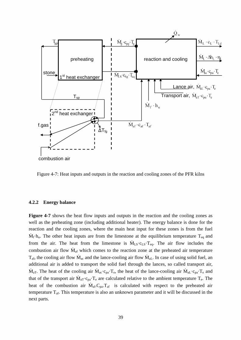
Figure 4-7: Heat inputs and outputs in the reaction and cooling zones of the PFR kilns

4.2.2 Energy balance Figure 4-7 shows the heat flow inputs and outputs in the reaction and the cooling zones as well as the preheating zone (including additional heater). The energy balance is done for the reaction and the cooling zones, where the main heat input for these zones is from the fuel Mf·hu. The other heat inputs are from the limestone at the equilibrium temperature Teq and from the air. The heat from the limestone is MLS·cLS·Teq. The air flow includes the combustion air flow Maf which comes to the reaction zone at the preheated air temperature Taf, the cooling air flow Mac and the lance-cooling air flow MaL. In case of using solid fuel, an additional air is added to transport the solid fuel through the lances, so called transport air, MaT. The heat of the cooling air Mac·cpa·Te, the heat of the lance-cooling air MaL·cpa·Te and that of the transport air MaT·cpa·Te are calculated relative to the ambient temperature Te. The heat of the combustion air Maf.Cpa.Taf is calculated with respect to the preheated air temperature Taf. This temperature is also an unknown parameter and it will be discussed in the next parts.

reaction and cooling preheating

2nd heat exchanger

ΔTfg

Transport air,

combustion air

Tsp

Lance air,

f.gas

stone

1st heat exchanger

40

The heat output is considered the same as the normal shaft kiln which includes the main heat consumed by the limestone decomposition ML·ΔhL·XL. The other heat outputs are the heat output with the lime ML·cL·TLd, with the gas Mg·cpg·Tg and the heat loss by the wall Qw. Then the energy balance in the PFR kiln can be determined as:

wgpggLLLLdLL

eqLSLSepaaTepaaLepaacafpaafuf

QTcMXhMTcM

TcMTcMTcMTcMTcMhM

+⋅⋅+⋅∆⋅+⋅⋅=

⋅⋅+⋅⋅+⋅⋅+⋅⋅+⋅⋅+⋅

(4-16)

In this equation the temperature T is taken in degree Celsius, oC. The combustion air mass flow is calculated as:

ffaf MLM ⋅⋅λ= (4-17) where λf is the excess air number, which represents the combustion air, it is also called as effective excess air number. This λf is smaller than the total excess air number, which will be defined in the next. The cooling air flow depends on the cooling air factor γac (m3

air/kglime).

Laacac MM ⋅ρ⋅γ= (4-18) with ρa is the density of the air at the ambient temperature. The lance-cooling air flow depends on the lance-cooling air factor γaL (m3

air/kglime).

LaaLaL MM ⋅ρ⋅γ= (4-19) The transport air flow depends on the transport air factor γaT (m3

air/kglime).

LaaTaT MM ⋅ρ⋅γ= (4-20) Then the total air flow blown into the kiln is summarized as:

ftotalaTaLacafa MLMMMMM ⋅⋅λ=+++= (4-21) while λtotal is the total excess air number.

41

The flue gas mass flow consists of the total air flow, the fuel flow and the CO2 flow produced by the calcination:

L2COfag MMMM ++= (4-22)

The CO2 flow produced by the decomposition is determined as before. Therefore, the energy consumption per kg of lime in the PFR kiln is obtained finally as:

( )

( ) ugpgfafpaf

L

wepaaaTaLaceqLS

2COgpg

2CO

2COLLLdL

h/]TcL1TcL[1MQ

TcTcy11Tc

y1y

XhTcE

⋅⋅⋅λ+−⋅⋅⋅λ+

+⋅⋅ρ⋅γ+γ+γ−⋅⋅−

−⋅⋅−

+⋅∆+⋅

=

(4-23) With the set of equations given previously, the energy consumption can be calculated iteratively. In Eq. (4-23) all values are now known except the gas temperature Tg and the preheated combustion air temperature Taf. The gas temperature Tg is determined by the way as same as the normal shaft kiln with introducing the temperature difference parameter ΔTeq at the ‘pinch’ point. The preheated combustion air temperature Taf is considered as a parameter for the calculation as well. This temperature will be defined as a function of the stone temperature in the preheating zone Tsp. The details of determination of Taf will be provided in the next paragraph. The limestone temperature in the preheating zone (the first heat changer) Tsp can be assumed as the gas temperature Tgp, which leaves the first heat exchanger to the second heat changer, Figure 4-7. This gas temperature Tgp is calculated from the energy balance in the first heat exchanger.

( ) ( )eeqLSLSgpgpgg TTcMTTcM −⋅⋅=−⋅⋅ (4-24)

The temperature Tsp (Tsp=Tgp) represents the limestone temperature in the preheating zone during the burning mode. Therefore, it depends on the alternative heat transfer in which the flue gas gives heat to the stone (in the non-burning mode) and then the stone transfers heat to the combustion air (in the burning mode). The temperature Tgp is also affected by the preheating zone length and the operating conditions. Then the energy consumption in Eq. (4-23) can be calculated, where the unknown parameter Taf is considered as a function of the limestone temperature Tsp by introducing the temperature difference ΔTfg defined as:

afspfg TTT −=∆ (4-25)

42

The temperature difference ΔTfg will be considered as a parameter for next calculations. This difference is affected by the heat transfer between the stone and the combustion air and the preheating zone length. The larger the heat transfer and the longer the preheating zone, the smaller the difference in temperature between the combustion air and the limestone. 4.2.3 Mass balance of CO2

Similar to the normal shaft kiln, the CO2 concentration in the burning shaft of the PFR kiln decides the temperature, at which the calcination begins. The CO2 is produced by the combustion of the fuel and the calcination of the limestone. The mass balance equation for the CO2 in the firing zone of the burning shaft is given by:

( ) bg2COL2COgfL2CO.

f2COgf.

xMMMxM ⋅+=+⋅ (4-26)

where f2COgf.

xM ⋅ is the mass flow of CO2 produced by the fuel combustion and L2CO.

M is the

mass flow of CO2 produced by the limestone decomposition. The combustion gas flow, which includes the combustion air and the fuel flow, is given as:

( ) fffafgf ML1MMM ⋅⋅λ+=+= (4-27)

The CO2 flow produced by decomposition is given by:

L2CO

2CO2COLSL2CO M

y1y

yMM ⋅−

=⋅= (4-28)

The lime mass flow ML can be replaced by the energy consumption E as before.

L

uf

MhME

⋅= (4-29)

Finally, the CO2 concentration in the firing zone of the burning shaft bg2COx is calculated.

( )

( ) u2CO

2COf

u2CO

2CO)f(f2COf

bg2CO

hy1

yL1E

hy1

yxL1E

x⋅

−+⋅λ+⋅

⋅−

+⋅⋅λ+⋅

=λ

(4-30)

43

From Eq. (4-30), it can be seen that the CO2 concentration in the burning shaft depends on the energy consumption E, the excess air number λf, the type of limestone 2COy and the kind of

fuel with hu and .

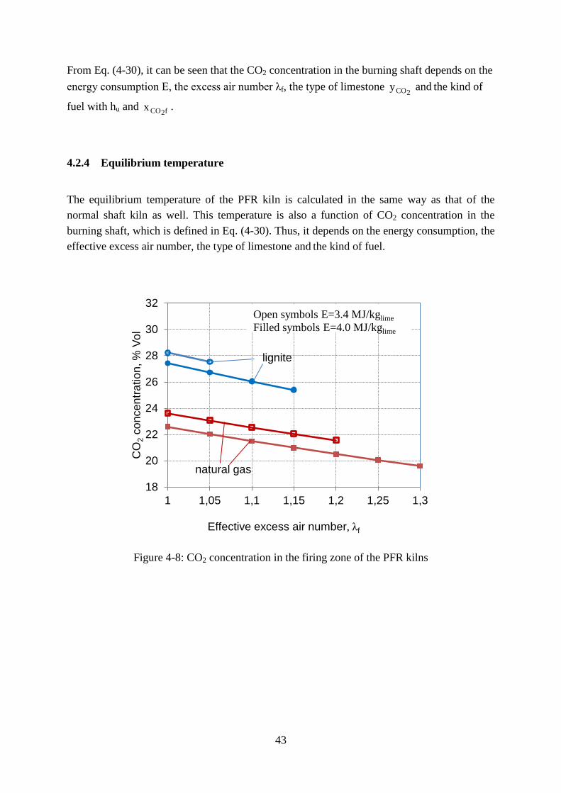
4.2.4 Equilibrium temperature

The equilibrium temperature of the PFR kiln is calculated in the same way as that of the normal shaft kiln as well. This temperature is also a function of CO2 concentration in the burning shaft, which is defined in Eq. (4-30). Thus, it depends on the energy consumption, the effective excess air number, the type of limestone and the kind of fuel.

Figure 4-8: CO2 concentration in the firing zone of the PFR kilns

f2COx

18

20

22

24

26

28

30

32

1 1,05 1,1 1,15 1,2 1,25 1,3

CO

2 con

cent

ratio

n, %

Vol

Effective excess air number, λf


lignite

natural gas

44

Figure 4-9: Starting calcination temperature in the firing zone of the PFR kilns

As an example, Figure 4-8 and Figure 4-9 show the CO2 concentrations and calcination temperatures for natural gas and lignite depending on the effective excess air number. The energy consumptions E = 3.4 MJ/kglime and E = 4.0 MJ/kglime that correspond to a relatively low and high value of energy usage were taken. The lower the energy consumption and the air excess number are, the higher the carbon dioxide concentration is. Lignite gives the higher CO2 in the gas phase. The lines for E = 3.4 MJ/kglime and E = 4.0 MJ/kglime for lignite end at λf = 1.05 and λf = 1.15, as for the higher excess air numbers, further low energy consumption is no more possible. It is remarkable here that the CO2 concentration in the flue gas and the equilibrium temperature in the PFR kilns are significantly lower than those in the normal shaft kilns. The reason is that the total excess air number in the PFR kilns is much higher since it includes the combustion air, the cooling air, the lance-cooling air and the transport air. As an example, Figure 4-10 shows some calculated values of the total excess air number in dependence on the effective excess air number. The calculations were done with natural gas fuel and the cooling air factor (γac) varying in the range of 0.6 - 0.7 m3

air/kglime. It can be seen from the figure that while the effective air number changes from 1.0 to 1.2, the total excess air number varies in the range from 1.75 to 2.1.

815

820

825

830

835

840

845

850

1 1,05 1,1 1,15 1,2 1,25 1,3

Cal

cina

tion

tem

p., o

C

Effective excess iar number, λf


lignite

natural gas

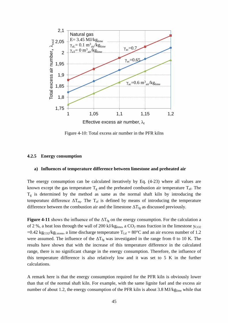
45

Figure 4-10: Total excess air number in the PFR kilns

4.2.5 Energy consumption

a) Influences of temperature difference between limestone and preheated air

The energy consumption can be calculated iteratively by Eq. (4-23) where all values are known except the gas temperature Tg and the preheated combustion air temperature Taf. The Tg is determined by the method as same as the normal shaft kiln by introducing the temperature difference ΔTeq. The Taf is defined by means of introducing the temperature difference between the combustion air and the limestone ΔTfg as discussed previously. Figure 4-11 shows the influence of the ΔTfg on the energy consumption. For the calculation a of 2 %, a heat loss through the wall of 200 kJ/kglime, a CO2 mass fraction in the limestone yCO2 =0.42 kgCO2/kgl.stone, a lime discharge temperature TLd = 80°C and an air excess number of 1.2 were assumed. The influence of the ΔTfg was investigated in the range from 0 to 10 K. The results have shown that with the increase of this temperature difference in the calculated range, there is no significant change in the energy consumption. Therefore, the influence of this temperature difference is also relatively low and it was set to 5 K in the further calculations. A remark here is that the energy consumption required for the PFR kiln is obviously lower than that of the normal shaft kiln. For example, with the same lignite fuel and the excess air number of about 1.2, the energy consumption of the PFR kiln is about 3.8 MJ/kglime while that

1,75

1,8

1,85

1,9

1,95

2

2,05

2,1

1 1,05 1,1 1,15 1,2

Tota

l exc

ess

air n

umbe

r, λ t

otal


Natural gas E= 3.45 MJ/kglime γaL= 0.1 m3

air/kglime γaT= 0 m3

air/kglime

γac=0.7

γac=0.65

γac=0.6 m3air/kglime

46

of the normal shaft kiln is almost 4.2 MJ/kglime. This reduction of the energy is a result of regenerative heat transfer arrangement in the PFR kilns, [43,44].

Figure 4-11: Energy consumption as function of temperature difference between stone and combustion air at the beginning of burning zone

b) Influences of types of fuel Figure 4-12 shows the energy consumption as a function of the kind of fuel and the effective excess air number. Calculations were done with three fuels natural gas, lignite and anthracite. The other inputs were kept the same as the previous calculation. It can be seen that at the same excess air number, the lignite fuel requires the highest energy consumption while the natural gas requires the lowest energy consumption. The energy consumption increases considerably with the increase of the excess air number.

3

3,1

3,2

3,3

3,4

3,5

3,6

3,7

3,8

0 2 4 6 8 10

Ene

rgy

in M

J/kg

lime

ΔTfg= Tsp - Taf

lignite

anthracite

natural gas

calacination enthalpy

2 % Res. CO2 λf=1.15 yCO2=0.42 TLd=80 oC ΔTeq=2 K qw=200 kJ/kglime

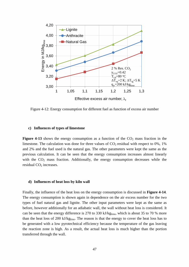
47

Figure 4-12: Energy consumption for different fuel as function of excess air number

c) Influences of types of limestone

Figure 4-13 shows the energy consumption as a function of the CO2 mass fraction in the limestone. The calculation was done for three values of CO2 residual with respect to 0%, 1% and 2% and the fuel used is the natural gas. The other parameters were kept the same as the previous calculation. It can be seen that the energy consumption increases almost linearly with the CO2 mass fraction. Additionally, the energy consumption decreases while the residual CO2 increases.

d) Influences of heat loss by kiln wall

Finally, the influence of the heat loss on the energy consumption is discussed in Figure 4-14. The energy consumption is shown again in dependence on the air excess number for the two types of fuel natural gas and lignite. The other input parameters were kept as the same as before, however additionally for an adiabatic wall, the wall without heat loss is considered. It can be seen that the energy difference is 270 to 330 kJ/kglime, which is about 35 to 70 % more than the heat loss of 200 kJ/kglime. The reason is that the energy to cover the heat loss has to be generated with a low pyrotechnical efficiency because the temperature of the gas leaving the reaction zone is high. As a result, the actual heat loss is much higher than the portion transferred through the wall.

3,00

3,20

3,40

3,60

3,80

4,00

4,20

1 1,05 1,1 1,15 1,2 1,25 1,3

Ene

rgy

in M

J/kg

lime


LigniteAnthraciteNatural Gas

2 % Res. CO2 yCO2=0.42 TLd=80 oC ΔTeq=2 K; ΔTfg=5 K qw=200 kJ/kglime

48

Figure 4-13: Energy consumption as function of mass fraction of CO2 in limestone

Figure 4-14: Energy usage with and without heat lost through the kiln wall

3,00

3,20

3,40

3,60

3,80

0,4 0,41 0,42 0,43 0,44

Ene

rgy

in M

J/kg

lime

Mass fraction of CO2 in kgCO2/kgLS

0%1%2%

Natural gas λf=1.15 TLd=80 oC ΔTeq=2 K ΔTfg=5 K qw=200 kJ/kglime

Res. CO2

3,00

3,20

3,40

3,60

3,80

4,00

4,20

1 1,05 1,1 1,15 1,2 1,25 1,3

Ene

rgy

in M

J/kg

lime


0 % Res. CO2 yCO2=0.42; TLd=80 oC ΔTeq=2 K,;ΔTfg=5 K

lignite

natural gas

qw=200 kJ/kglime qw=0 kJ/kglime

49

4.3 Conclusions The theoretical minimum values of the specific energy consumptions required for the normal shaft kilns and the PFR kilns are determined in this chapter. The energy consumption depends on the following parameters:

• The conversion degree of lime or residual CO2: The higher the lime conversion degree (lower residual CO2), the higher the energy consumption

• The type of limestone: E.g., the higher the mass fraction of CO2 in limestone (more CaCO3), the more the energy required

• The types of fuel: E.g., the lower the heating value of the fuel, the higher the energy consumption

• The excess air number: The larger the excess air number, the more energy consumption required

• The temperature difference between the gas and solid at the ‘pinch’ point: The higher the temperature difference, the higher the energy consumption

• The alternative heat transfer from the flue gas to the limestone and to the combustion air (PFR kilns only): The better the heat transfer process (the higher the preheated combustion air temperature), the lower the energy consumption

Results of calculations have revealed that due to the regenerative heat transfer (reusing the flue gas for preheating the limestone), the energy consumption required for the PFR kilns is significantly lower than that of the normal shaft kilns. In the above calculations of the energy consumption, it was assumed that the lime discharge temperature, the flue gas temperature, the residual CO2 and the heat loss are known as inputs for calculations. However, they are strongly affected by operating conditions of the burning process. Therefore, they must be determined by mathematical modeling, which will be presented in the next chapters.

50

5 Simulation of lime calcination in normal shaft kiln 5.1 Mathematical model

5.1.1 Energy balance equation

a) Preheating and cooling zone

The energy balance is established for the gas (g) and the solid (s) in a section of kiln length dz, Figure 5-1. In the preheating and the cooling zones, the solid particles are heated up and cooled down by the gas, thus these two zones can be considered as heat exchangers. The energy balance equations are described as:

Figure 5-1: Scheme of normal shaft kilns with a section length dz

• For the gas

( ) ( ) ( )dz

QdTT1OA

dzdT

cM )z(w

.

sgFz)z(g

pgg.

−−⋅ψ−⋅⋅⋅α=⋅ κ⋅ (5-1)

The change of the gas enthalpy flow is equal to the heat transferred between the gas and the solid and the local wall heat loss.

dz

solidin

solidout gasin

gasout

51

• For the solid

( ) ( ) ( )gsFz)z(s

pss.

TT1OAdz

dTcM −⋅ψ−⋅⋅⋅α=⋅ κ⋅ (5-2)

The change of the solid enthalpy flow is equal to the heat transferred between the gas and the solid. Here M represents the mass flow, cp the specific heat capacity, T the temperature, ακ the overall heat transfer coefficient, AF the cross-sectional area of the furnace, O the specific surface of the stones in m2/m3, ψ the void fraction of the bed and Qw the local wall heat loss. It is known that the heating-up or the cooling-down of solid particles is a transient process, in which a solid particle has a temperature distribution in a radical direction. However, to simplify for the energy balance, the solid temperature is considered as the mean value. Therefore, in the above equations the overall heat transfer coefficient is used.

In Eq.(5-1), the local wall heat loss (Qw) is due to the heat loss by conduction (Qwλ) through the wall, which is determined (e.g., for a circular cross-section) as:

)R/Rln(/)TT(LR2Q inw)z(kw)z(kiww)z(w

.−⋅λ⋅π=λ

(5-3)

with λw is the wall thermal conductivity, Rin and Rw are the kiln inner and outer radius, Tki and Tkw are the wall inner and outer temperatures, Figure 5-2. The Tki is assumed as the gas temperature Tg, and Tkw is calculated from the heat balance at the wall surface as:

( )4)z(kwe)z(kwww)z(wr

.

)z(wc

.

)z(w

.T)TT(LR2QQQ ⋅ε⋅σ+−⋅α⋅π=+=λ

(5-4)

where (Qwc) and (Qwr) are the heat flows by convection and radiation from the wall surface to the ambience, αw is the convective heat transfer coefficient (for the air), σ the Stefan-Boltzmann constant and ε the wall emissivity. The total wall heat loss is obtained by taking integral the local wall heat loss along the kiln axis.

52

Figure 5-2: Heat transfer at the kiln wall of shaft kilns

b) Reaction zone

• For the gas

( ) ( ) ( )dz

QdTT1OAh

dzMdTcM

dzd )z(w

.

swgFzu)z(f

.

)z(gpg)z(g.

−−⋅ψ−⋅⋅⋅α−⋅=

⋅⋅ (5-5)

• For the solid

( ) ( ) ( ) 2CO)z(2CO

.

swgFz)z(swps)z(s.

hdz

MdTT1OATcMdzd

∆⋅−−⋅ψ−⋅⋅⋅α=

⋅⋅ (5-6)

In Eq. (5-5), the change of the gas enthalpy flow is equal to the local heat produced by the fuel combustion minus the heat transferred from the gas to the solid and the local wall heat loss. Here Mf means the mass flow of the fuel, hu the calorific heating value of the fuel, α the convective heat transfer coefficient, Tsw the surface temperature of the solid particle.

Qwλ Qwr

Qwc

Refractory Insulation

Limestone Particles

Gas phase

Tkw

Te

Tki

Rin R

w

53

In Eq. (5-6), the change of the solid enthalpy flow is equal to the heat transferred from the gas and the heat consumed by the decomposition. Here MCO2 and ΔhCO2 are the mass flow and the specific reaction enthalpy with respect to decomposed CO2. A remark from this equation is that the heat consumed by calcination is much higher than the solid enthalpy flow. Therefore, the change of the mean temperature of the solid is approximated by the change of the surface temperature. This surface temperature is used to calculate the heat transfer in this zone. The kinetics of the combustion behavior and the flame length in shaft kilns is unknown since it is very complex to describe. It depends on the kind of fuel and the type of kiln. Therefore, the heat of the combustion in Eq. (5-5) is treated in a simplified way, in which the fuel combustion is described corresponding to a given fuel burning degree Xf.

dzdX

Mdz

Md )z(ff

.)z(f.

⋅= (5-7)

The burning degree Xf is approximated by a function with initial conditions Xf =0 at the beginning of the flame (burner level, zb) and Xf = 1 at the end of the flame (zr), Figure 5-3. The function of Xf is given as:

))zz(aexp(1X bb)z(f −⋅−= (5-8)

where a and b are factors used to adjust the flame length Lf (Lf = zb-zr), which depends on the kinds of fuel and kilns. If the Xf(zr) is taken as 0.9999, the factor a is obtained from Eq.(5-8) in dependence on b and Lf as:

bfb )Lz()10ln(4a

−= (5-9)

In Eq. (5-6), the mass flow of the CO2 decomposed in the length dz is calculated as:

dtMd

w1

dzMd 2CO

.

s

)z(2CO.

⋅= (5-10)

where ws is the stone velocity and dMCO2/dt is the mass flow of the CO2 decomposed in the time dt, which is determined as before in chapter 3. The stone velocity ws is calculated as:

FL

L.

s A1Mw ⋅

ρ= (5-11)

with ML and ρL are the flow and the density of the lime.

54

Tem

pera

ture

Axial position

Tair

Tgas

Tsolid

Ta.in

Tg.mix

Ts.in

Tgo

z=0 z=zr z=zb z=L

air stone

preheating reaction cooling

Xf

Top Bottom

Lf

Xf=1

Xf=0

fuel / air

Figure 5-3: Temperature and fuel burning profiles in a normal shaft kiln

5.1.2 Mass balance equation The mass flows of the gas and the solid in the preheating and the cooling zones are constant. However, in the reaction, due to the limestone decomposition, the mass flow of the gas and that of the solid change. The mass balance equations for the gas and the solid in the reaction zone are given as: • For the gas

)z(2CO.

a.

f.

)z(g.

MMMM ++= (5-12)

The gas flow includes the flows of the fuel, the air and the CO2 produced by the decomposition. • For the solid

)z(2CO.

LS.

)z(s.

MMM −= (5-13)

The solid flow decreases since the CO2 is dissociated from the solid to the gas.

55

5.1.3 Boundary value problem and numerical solution The system of ordinary differential equations describing the energy conservations needs to be solved numerically to get temperature profiles. Initial values for solving these equations are given as: Ts (z=0) = Ts.in (5-14)

Tg (z=L) = Ta.in (5-15)

Here the initial values are given at the kiln top (z=0) with the stone inlet temperature (Ts.in) and at the kiln bottom (z=L) with the air inlet temperature (Ta.in), Figure 5-3. These initial values are at two points of the solution domain, thus numerical solutions face typical problems. These problems are so called boundary value problems. The boundary value problem is considered as one of the most difficult problems for simulations of lime burning in shaft kilns, which have also been reported by other authors [4546 47- 48 4950].51,52 To be more convenient and effective for developing numerical solutions, the preheating and the reaction zones are handled together while the cooling zone is calculated separately. For calculating the preheating and the reaction zones, the initial value of the gas temperature (Ta.in) in Eq.(5-15) is replaced by Tg.mix; the temperature of the mixture of fuel / secondary air and cooling air at the burner level (zb). Tg (z=zb) = Tg.mix (5-16) In general, the Runge-Kutta method is employed to solve differential equations in which the initial values are normally given at one point of the solution domain. However, due to the boundary value problem it is not possible to apply in this case. Therefore, numerical solutions can be employed by incorporating the shooting method with the help of the Runge-Kutta method. Nevertheless, the equations describe the complex of heat and mass transfer and chemical reactions while all of them are coupled so that the solution must be good enough to minimize errors of every single integration step in the solution domain. In this study, some commercial solvers, for example, bvp4c (a MATLAB code), which is able to solve the boundary value problem, are also used. The shooting method is a numerical solution for solving the boundary value problem by reducing it to the solution of an initial value problem. The solution is based on a shooting progress where the program is employed to target an objective from a given position in the solution domain. For example, to calculate the gas temperature in the preheating and reaction zones where the gas temperature Tg.mix is known at the end of the reaction zone (burner level), different values of Tgo at the kiln top must be given as starting points, then the program will

http://en.wikipedia.org/wiki/Boundary_value_problem

http://en.wikipedia.org/wiki/Initial_value_problem

56

try to target the initial value Tg..mix. After succeeding to reach the Tg.mix, a final value of the Tgo is calculated and a gas temperature profile is determined as well. As mentioned before, the commercial solver bvp4c is also used for developing the numerical solution. This is a finite difference code, which implements the 3-stage Lobatto IIIa formula. The code provides continuous solution with fourth-order accuracy uniformly in the interval of integration. The solution is done in the solution domain with two point boundary conditions where mesh selection and error control are based on the residual of the continuous solution. Error! Reference source not found. show flowcharts of the numerical solutions developed by using the commercial solver bvp4c.

To understand the behavior of the differential equations, sensitivity analysis of the numerical solution was done by using the two above methods. The results obtained by both numerical methods are similar. However, sometime the numerical solutions become sensitive while verifying inputs of the equations. The following variables have been reported with significant effects on the sensitivity of the solutions.

• The starting / initial values: Tgo, Tg.mix, Ts.in, Ta.in • The operating parameters: Energy input, kiln throughput, particle size etc. • The kiln dimension: Height, diameter

It is difficult to conclude the reasons that cause the solution to become sensitive. The first reason is the boundary value problem. The second reason is the complex coupling of the heat and mass transfer and chemical reactions in the differential equations. From a mathematical point of view, the third reason is that the systems of differential equations have ‘stiff’ equations or non-unique equations, which typically cause instability for numerical solutions. In this dissertation, to make the numerical solution methods easier, the following assumptions are made.

• The conditions at every cross-section along the kiln axis are homogeneous • All stone particles are considered as spheres with the same size • The radiative heat transfer is neglected • The combustion of the fuel is treated in a simplified way with a given burning profile • The gas is considered as an ideal mixture containing N2, O2, CO2 and H2O

57

Figure 5-4: Numerical solution with using commercial solver bvp4c in MATLAB

start

Assume gas temp., at the burner level Tg.mix

Calculation preheating and reaction zone

Energy balances ?

Y

Input parameters

Output results

N

End

Modify Tg.mix

Calculation cooling zone

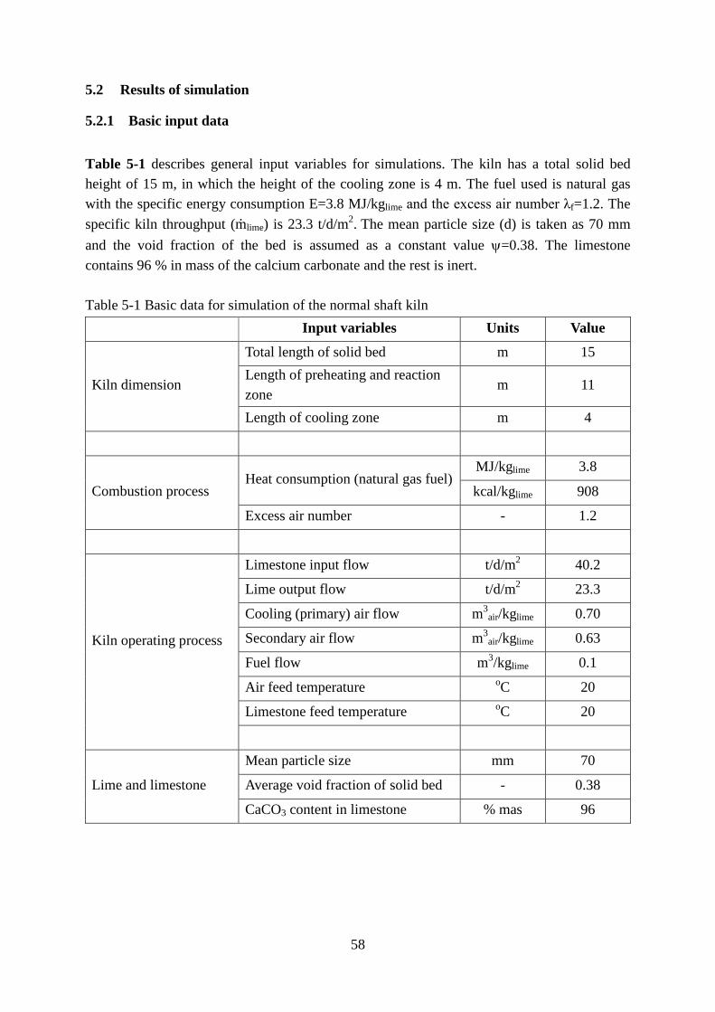
58

5.2 Results of simulation

5.2.1 Basic input data Table 5-1 describes general input variables for simulations. The kiln has a total solid bed height of 15 m, in which the height of the cooling zone is 4 m. The fuel used is natural gas with the specific energy consumption E=3.8 MJ/kglime and the excess air number λf=1.2. The specific kiln throughput (mlime) is 23.3 t/d/m2. The mean particle size (d) is taken as 70 mm and the void fraction of the bed is assumed as a constant value ψ=0.38. The limestone contains 96 % in mass of the calcium carbonate and the rest is inert. Table 5-1 Basic data for simulation of the normal shaft kiln

Input variables Units Value

Kiln dimension

Total length of solid bed m 15 Length of preheating and reaction zone

m 11

Length of cooling zone m 4

Combustion process Heat consumption (natural gas fuel)

MJ/kglime 3.8

kcal/kglime 908

Excess air number - 1.2

Kiln operating process

Limestone input flow t/d/m2 40.2

Lime output flow t/d/m2 23.3

Cooling (primary) air flow m3air/kglime 0.70

Secondary air flow m3air/kglime 0.63

Fuel flow m3/kglime 0.1

Air feed temperature oC 20

Limestone feed temperature oC 20

Lime and limestone

Mean particle size mm 70

Average void fraction of solid bed - 0.38

CaCO3 content in limestone % mas 96

59

5.2.2 Principal temperature and conversion profile Figure 5-5 shows the principal temperature and the mass fraction profiles in the normal shaft kiln with basic data given in Table 5-1. The mass fraction is defined as the mass ratios of the gas or the solid to the lime, kg/kglime. Figure 5-5 is illustrated in the horizontal direction, which is transferred corresponding to the schematic diagram of the normal shaft kiln shown before in Figure 1-1. The coordinate 0 m represents the top of the kiln. Initially, the limestone is charged into the kiln from the top at the ambient temperature of 20 oC. Then it is preheated by the hot gas in the preheating zone and its temperature increases rapidly until the reaction temperature (820oC) at about 3.1 m. At this position, the limestone decomposition begins and its mass fraction starts decreasing. The end of the preheating zone indicates the beginning of the reaction zone. In the reaction zone, both the solid surface (Tsw) and core (Tsf) temperatures are depicted together. At the end of this zone (11 m), the fuel and the secondary air are injected at the ambient temperature, and then they mix with the hot air coming from the cooling zone. The gas mixture has an average temperature of about 700 oC, which is lower than that of the solid. When the gas temperature is lower than that of the solid, the decomposition process is not possible since the gas cools the solid. The combustion is assumed to start immediately from the end of the reaction zone, thus the gas temperature increases sharply and it exceeds the solid temperature at about 10.6 m. As a result, the gas, on the way to the kiln top, transfers heat to the solid and the decomposition process is possible. The calcination zone lies from 3.1 m to 10.6 m. The solid, on the way to the kiln bottom, gets heat from the combustion gas; therefore, its temperature keeps increasing in the reaction zone until it reaches a maximum value of about 1432 oC at 10.6 m. The solid leaves the reaction zone with a temperature of about 1080 oC and then enters the cooling zone, where it is cooled down by the cooling air until it reaches discharge temperature. In the cooling zone, the heat capacity ratio of the lime to the air is assumed as one, thus both temperature profiles are linear.

60

Figure 5-5: Principal temperature and mass fraction profiles in the normal shaft kilns

In addition, other characteristic values of this simulation are summarized in Table 5-2. The temperature of the flue gas is 308 oC and that of the lime discharge is 80 oC. A remark here is that these temperatures are considered as mean values obtained directly at the top / bottom of the solid bed. Measured values are often lower since the gas at the top is mixed with false air and the lime temperature is detected only after discharge. The maximum temperature of the gas is 1468 °C and that of the solid is 1432 °C. The heat loss through the kiln wall is about 6.2 % of the total energy input and the pressure drop is 202 mbar.

0

400

800

1200

0 3 6 9 12 15

Tem

pera

ture

in o C

Axial position in m

Tg

Tsw

Tsf

1500

Ta

a)


1

1,25

1,5

1,75

2

2,25

2,5

0 3 6 9 12 15

Mas

s fra

ctio

n in

kg/

kglim

e

Axial position in m

gas

solid

b)

Natural gas E=3.8 MJ/kglime mlime= 23.3 t/d/m2

d=70 mm λf=1.2

.

61

Table 5-2 Simulation results of the normal shaft kiln

Outputs Unit Value

Flue gas temperature oC 308

Lime discharge temperature oC 80

Calcination starts at m 3.1

Calcination length m 7.5

Lime conversion % 100

Maximum gas temperature oC 1468

Maximum solid temperature oC 1432

Heat loss by kiln wall % 6.2

Total pressure drop mbar 202

5.2.3 Pressure drop profile Figure 5-6 reveals a typical pressure drop profile along the normal shaft kiln. Simulations were done with the mean particle size of 70 mm, the average kiln void fraction of 0.38 and the gas property depending on the gas temperature simulated as before.

Figure 5-6: Principal pressure drop profile along the normal shaft kilns

0

50

100

150

200

250

0 3 6 9 12 15

ΔP

in m

bar

Axial position in m


E=3.8 MJ/kglime mlime= 23.3 t/d/m2

d=70 mm Ψ=0.38

62

As seen from Table 5-2, the total pressure drop of the kiln is about 202 mbar, however the pressure drop is different in every zone. For instance, in the cooling zone it is relatively small due to low gas flow (only cooling air). In the burning and preheating zones, the pressure drop is much higher due to two reasons: a) the gas flow is much higher because the fuel, the secondary air and the decomposed CO2 are all added in these zones, b) the kiln temperature is also higher. 5.3 Influencing parameters 5.3.1 Influence of energy input Figure 5-7 shows the temperature and the conversion (solid mass fraction) profiles for different energy inputs. As an example, the energy input was varied in the range from 3.7 to 3.9 MJ/kglime. Other input parameters for simulations were kept the same as given before in Table 5-1. The higher the energy input, the more fuel is introduced, thus the more heat is generated by the combustion. This causes an increase of the gas and the solid temperatures. As a result, the limestone decomposes faster and requires a shorter calcination zone. A higher energy results in a shorter preheating zone and an earlier beginning of the calcination process. In addition, Table 5-3 summarizes the characteristic values of simulations. It can be seen that an increase of the energy results in an increase of the flue gas and the lime discharge temperatures. However, the flue gas temperature changes in a stronger way. The maximum temperatures of the gas and the solid also increase significantly with the increase of the energy. A decrease of the energy extends the length of the calcination zone since the temperature decreases. For instance, with a decrease of energy until 3.7 MJ/kglime, the calcination zone becomes so long, thus a complete calcination is not possible. Furthermore, the more fuel is injected, the more air is required (higher gas flow), which results in a higher pressure drop.

63

Figure 5-7: Influence of energy input on the temperature and the conversion profiles

0

400

800

1200

1600

0 3 6 9 12

Gas

tem

p., i

n o C

2

1

3

1. E=3.9 MJ/kglime 2. E=3.8 MJ/kglime 3. E=3.7 MJ/kglime

a)

preheating reaction

0

400

800

1200

1600

0 3 6 9 12

Sol

id te

mp.

, in

o C

2

1

3

b)

mlime=23.3t/d/m2

d=70 mm λf=1.2

.

1

1,2

1,4

1,6

1,8

0 3 6 9 12

Sol

id m

ass

fract

., in

kg/

kglim

e

Axial position in m

1

2

3

c)

64

Table 5-3 Influence of energy input

Energy input MJ/kg 3.7 3.8 3.9

Flue gas temperature oC 301 308 338

Lime discharge temp. oC 76 80 98

Calcination start at m 3.4 3.1 2.2

Calcination length m 7.6 7.5 6.9

Lime conversion % 98.8 100 100

Max. gas temperature oC 1398 1468 1565

Max. solid temperature oC 1352 1432 1519

Total pressure drop mbar 180 202 236

5.3.2 Influence of lime throughput Figure 5-8 and Table 5-4 show the simulations for different kiln throughputs in the same manner as before. As an example, the kiln throughput was changed in the range of 23.3 ± 2 t/d/m2. Other input parameters such as the energy were kept the same as before. A lower kiln throughput leads to a longer residence time of the limestone. Consequently, the limestone gets more time to decompose, thus the calcination zone becomes shorter. The kiln temperature decreases with the increase of the throughput. Therefore, in order to get the same conversion degree (e.g., complete calcination) the length of the calcination zone must be extended. If this length is not sufficient, a complete calcination cannot be achieved. For instance, in this simulation, an incomplete calcination is observed with 25 t/d/m2 throughput.

Table 5-4 Influence of lime throughput

Lime throughput t/d/m2 21.3 23.3 25.3



Calcination starts at m 2.5 3.1 3.2


Lime conversion % 100 100 98.6




65

Figure 5-8: Influence of kiln throughput on the temperature and the conversion profiles

0

400

800

1200

1600

0 3 6 9 12

Gas

tem

p., i

n o C

1

2 3

1. mlime=21.3 t/d/m2

2. mlime=23.3 t/d/m2 3. mlime=25.3 t/d/m2

preheating reaction

a)

.

.

.

0

400

800

1200

1600

0 3 6 9 12

Sol

id te

mp.

, in

o C

1

2

3

b)

E=3.8MJ/kglime d= 70 mm λf = 1.2

1

1,2

1,4

1,6

1,8

0 3 6 9 12

Sol

id m

ass

fract

., n

kg/k

g lim

e

Axial position in m

1

2 3

c)

66

The incomplete calcination causes the increases of the flue gas and the lime discharge temperature, Table 5-4. The reason is that a small amount of heat produced by the combustion, which is not consumed by the calcination, is transferred to the flue gas and the lime discharge. Additionally, a higher kiln throughput leads to a higher gas flow, thus it results in a higher pressure drop. A remark is observed that the kiln throughput affects the maximum temperature of the solid bed. Therefore, it has an indirect effect on the lime reactivity. The lower the kiln throughput, the higher the maximum temperature is and the lower the expected reactivity of lime is. 5.3.3 Influence of particle size Figure 5-9 and Table 5-5 show the simulation results for different particle sizes. As mentioned before, here the particle size represents the mean value of a distribution. Simulations were done for three sizes of 65, 70 and 75 mm while other inputs were kept the same as before. A smaller particle decomposes faster and requires a shorter calcination zone. An increase of the particle size requires an extension of the calcination zone. A complete calcination cannot be obtained with large particle sizes if the length for calcination is not sufficient. For instance, in this simulation, an incomplete calcination is observed with the size of 75 mm. The larger the stone size, the longer the preheating zone is required. In addition, the kiln maximum temperatures and the pressure drop increase considerably with the decrease of the particle size, Table 5-5.

Table 5-5 Influence of particle size

Particle size mm 65 70 75









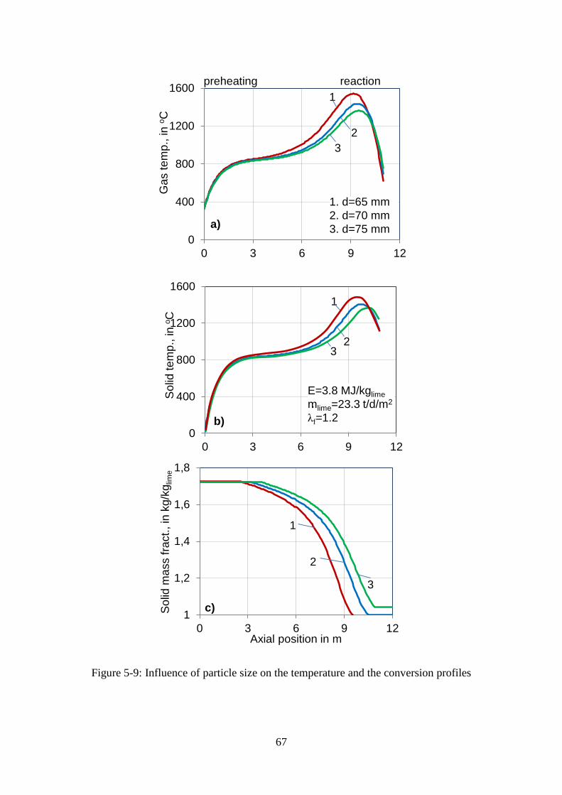
67

Figure 5-9: Influence of particle size on the temperature and the conversion profiles

0

400

800

1200

1600

0 3 6 9 12

Gas

tem

p., i

n o C

1

2 3

1. d=65 mm

2. d=70 mm 3. d=75 mm

preheating reaction

a)

0

400

800

1200

1600

0 3 6 9 12

Sol

id te

mp.

, in

o C 1

2 3

b)

E=3.8 MJ/kglime mlime=23.3 t/d/m2

λf=1.2 .

1

1,2

1,4

1,6

1,8

0 3 6 9 12

Sol

id m

ass

fract

., in

kg/

kglim

e

Axial position in m

1

2

3

c)

68

5.3.4 Influence of limestone origin To see how the material properties influence the process, simulations were done for three different kinds of limestones, which have different properties as shown before in Table 3-2. The simulation results are shown in Figure 5-10 and Table 5-6. The limestone (Ge.1) with the highest reaction coefficient decomposes with the highest calcination rate and requires the shortest calcination zone. In contrast, the limestone (Ge.3) with the smallest reaction coefficient decomposes with the lowest calcination rate and needs the longest calcination zone. It is remarkable that with the same operating conditions, the limestone Ge.3 does not completely decompose. Therefore, to get complete calcination for this limestone, higher energy input or lower kiln throughput are required.

Table 5-6 Influence of limestone property

Limestone - Ge.1 Ge.2 Ge.3









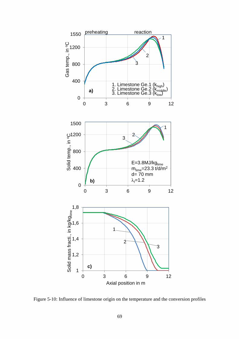
69

Figure 5-10: Influence of limestone origin on the temperature and the conversion profiles

0

400

800

1200

0 3 6 9 12

Gas

tem

p., i

n o C

2

1

1. Limestone Ge.1 (khigh) 2. Limestone Ge.2 (kmiddle)

3. Limestone Ge.3 (klow)

a)

1550 preheating reaction

3

0

400

800

1200

0 3 6 9 12

Sol

id te

mp.

, in

o C

3 2

1

b)

1500

E=3.8MJ/kglime mlime=23.3 t/d/m2

d= 70 mm λf=1.2

.

1

1,2

1,4

1,6

1,8

0 3 6 9 12

Sol

id m

ass

fract

i., in

kg/

kglim

e

Axial position in m

1

2 3

c)

70

5.3.5 Influence of excess air number Figure 5-11 and Table 5-7 show the simulation results for different excess air numbers varied in the range from 1.2 to 1.4. A smaller excess air number causes a higher kiln temperature, leading to a shorter calcination zone. An increase of the excess air number results in an increase of the calcination zone since the kiln temperature decreases. With an increase of the excess air number up to 1.4, the temperature becomes so low that the length of calcination is not sufficient to obtain a complete calcination. Additionally, an increase of the excess air number results in a higher gas flow, thus it causes a greater pressure drop. [53, 54, 55]

Table 5-7 Influence of excess air number

Excess air number - 1.1 1.2 1.3









71

-

Figure 5-11: Influence of excess air number on the temperature and the conversion profiles

0

400

800

1200

1600

0 3 6 9 12

Gas

tem

p., i

n o C

2

1

3

1. λf=1.1 2. λf=1.2 3. λf=1.3

a)

preheating reaction

0

400

800

1200

0 3 6 9 12

Sol

id te

mp.

, in

o C

2

1

3


d= 70 mm

b)

1500

.

1

1,2

1,4

1,6

1,8

0 3 6 9 12

Sol

id m

ass

fract

., in

kg/

kglim

e

Axial position in m

1

2

3

c)

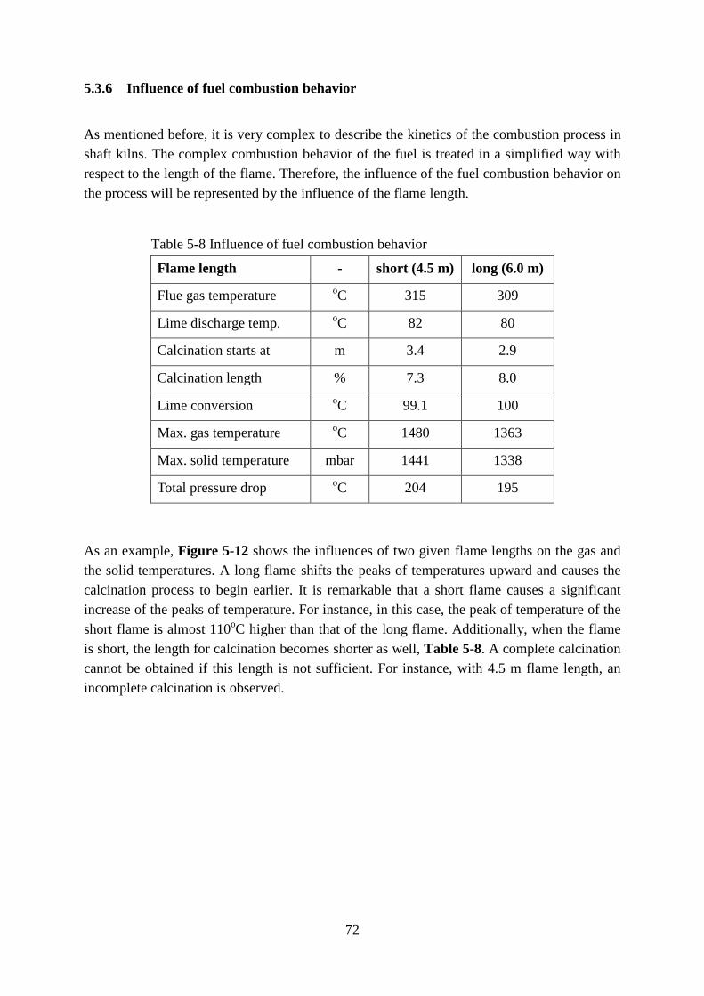
72

5.3.6 Influence of fuel combustion behavior

As mentioned before, it is very complex to describe the kinetics of the combustion process in shaft kilns. The complex combustion behavior of the fuel is treated in a simplified way with respect to the length of the flame. Therefore, the influence of the fuel combustion behavior on the process will be represented by the influence of the flame length.

Table 5-8 Influence of fuel combustion behavior

Flame length - short (4.5 m) long (6.0 m)

Flue gas temperature oC 315 309

Lime discharge temp. oC 82 80

Calcination starts at m 3.4 2.9

Calcination length % 7.3 8.0

Lime conversion oC 99.1 100

Max. gas temperature oC 1480 1363

Max. solid temperature mbar 1441 1338

Total pressure drop oC 204 195

As an example, Figure 5-12 shows the influences of two given flame lengths on the gas and the solid temperatures. A long flame shifts the peaks of temperatures upward and causes the calcination process to begin earlier. It is remarkable that a short flame causes a significant increase of the peaks of temperature. For instance, in this case, the peak of temperature of the short flame is almost 110oC higher than that of the long flame. Additionally, when the flame is short, the length for calcination becomes shorter as well, Table 5-8. A complete calcination cannot be obtained if this length is not sufficient. For instance, with 4.5 m flame length, an incomplete calcination is observed.

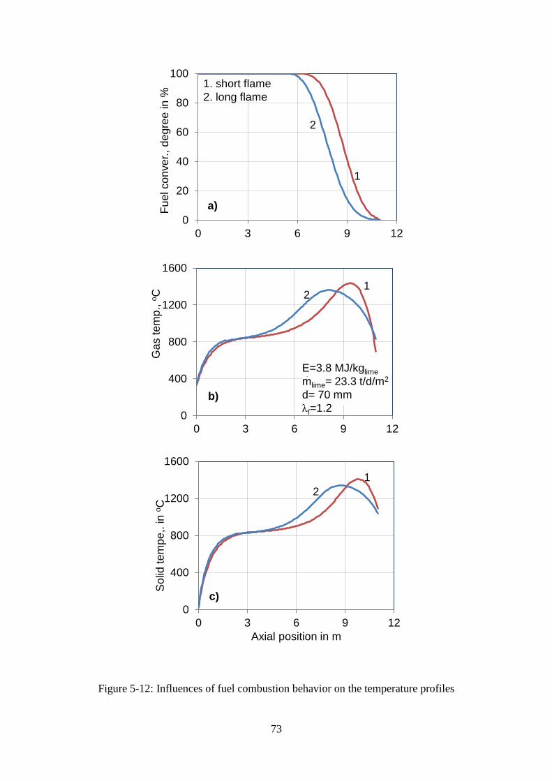
73

Figure 5-12: Influences of fuel combustion behavior on the temperature profiles

0

20

40

60

80

100

0 3 6 9 12

Fuel

con

ver.,

deg

ree

in %

1

2

1. short flame 2. long flame

a)

0

400

800

1200

1600

0 3 6 9 12

Gas

tem

p., o

C 1

2


d= 70 mm λf=1.2

b)

.

0

400

800

1200

1600

0 3 6 9 12

Sol

id te

mpe

,. in

o C

Axial position in m

2 1

c)

74

6 Simulation of lime calcination in PFR kiln 6.1 Simplification of PFR kiln for modeling The PFR kiln consists of two shafts connected by a channel as shown before in Figure 1-3. Each shaft is subjected to two distinct modes of operations, burning and non-burning mode, in which the periodic time for each mode is about 8 – 15 min. On the one hand, for the process modeling, it is very difficult to describe mathematically the periodic transient behavior. On the other hand, it gives no more information to the expected results as mentioned in the introduction. Therefore, if the reversal time between two shafts can be assumed extremely short, then the non-burning shaft can be simplified as pipes located inside the burning shaft. These pipes act as heat exchangers for the heat transfer process between the gas (from non-burning shaft) and the solid. Two shafts can be simplified as one shaft, which is shown in Figure 6-1. The new shaft has three typical operating zones as before with the preheating, the burning and the cooling zones. In this dissertation, the mathematical model will be developed with respect to the simplified shaft. Therefore, the mean values of the periodic fluctuations are considered. 6.2 Mathematical model

6.2.1 Energy balance equation

a) Preheating and cooling zone

In the cooling zone, the energy balance equations are described by the same way as given before, Eq(5-1)-(5-2). In the preheating zone, there are two heat transfer processes: a) from the flue gas (fg) to the solid, and b) from the solid to the combustion air (a). The energy balance equations for the combustion air and the flue gas are also described by the same way as before, Eq(5-1). The solid involves in two heat transfer processes, thus its energy balance equation is described as:

( ) ( ) ( ) ( )asF)z(a.sfgF)z(fg.)z(s

pss.

TT1OATT1OAdz

dTcM −⋅ψ−⋅⋅⋅α−−⋅ψ−⋅⋅⋅α=⋅⋅ κκ (6-1)

The change of the solid enthalpy flow is equal to the heat transferred from the flue gas to the solid and the heat transferred from the solid to the combustion air. Here ακ.fg and ακ.a are the overall heat transfer coefficient with respect to the flue gas and the combustion air.

75

Figure 6-1: Simplification of the PFR shaft kilns

air lime

fuel

pipe

limestone

lime

gas

air

fuel

bu

rnin

g sh

aft

no

n-bu

rnin

g sh

aft

simplify

limestone

air gas

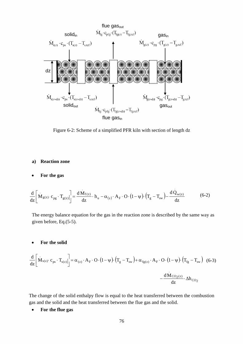
76

Figure 6-2: Scheme of a simplified PFR kiln with section of length dz

a) Reaction zone

• For the gas

( ) ( ) ( )dz

QdTT1OAh

dzMdTcM

dzd )z(w

.

swgFzu)z(f

.

)z(gpg)z(g.

−−⋅ψ−⋅⋅⋅α−⋅=

⋅⋅ (6-2)

The energy balance equation for the gas in the reaction zone is described by the same way as given before, Eq.(5-5).

• For the solid

( ) ( ) ( ) ( )swfgF)z(fgswgF)z()z(sps)z(s.

TT1OATT1OATcMdzd

−⋅ψ−⋅⋅⋅α+−⋅ψ−⋅⋅⋅α=

⋅⋅ (6-3)

2CO)z(2CO

.

hdz

Md∆⋅−

The change of the solid enthalpy flow is equal to the heat transferred between the combustion gas and the solid and the heat transferred between the flue gas and the solid. • For the flue gas

solidin

solidout

flue gasin

gasin

gasout

dz

flue gasout

77

( ) ( ) ( )swfgFzfg)z(fgpfgfg.

TT1OATcMdzd

−⋅ψ−⋅⋅⋅α=

⋅⋅ (6-4)

The change of the enthalpy flow of the flue gas is equal to heat transferred between the flue gas and the solid.

6.2.2 Mass balance equation Similar to the normal shaft kiln, the mass balance equations are described for the reaction zone as a representative case since the mass flows of the gas and the solid change in this zone due to the limestone decomposition. • For the gas (burning shaft)

)z(2CO.

aT.

af.

f.

)z(g.

MMMMM +++=

(6-5) The gas flow includes the fuel flow, the combustion air flow Maf, the transport air flow MaT (for solid fuel) and the decomposed CO2 flow. The gas flow changes due to the CO2 flow produced by the limestone decomposition. • For the solid

)z(2CO.

LS.

)z(s.

MMM −=

(6-6) The mass balance equation for the solid is given as before in Eq.(5-13). • For the flue gas (non-burning shaft)

aL.

ac.

g.

fg.

MMMM ++= (6-7)

The flue gas flow is constant along the kiln. It includes the total gas flow from the burning shaft Mg, the total cooling air flow Mac and the lance cooling air flow MaL.

6.2.3 Boundary value problem and numerical solution

78

Similar to the normal shaft kilns, the initial values for solving the system of ordinary differential equations are given with the stone inlet temperature Ts.in and the combustion inlet air temperature Taf.in at the kiln top (z=0) and with the cooling air inlet temperature Tac.in at the kiln bottom (z=L), Figure 6-3. Tg (z=0) = Taf.in (6-8)

Ts (z=0) = Ts.in (6-9)

Tfg (z=L) = Tac.in (6-10) In this case, numerical solutions face again the boundary value problems. As mentioned before, to be easier for numerical solutions, the preheating and reaction zones are handled together while the cooling zone is calculated separately. With calculating the preheating and the reaction zones, the initial value of the gas temperature is given by Tg.mix, which is the temperature of the gas mixture at the crossover-channel (zchannel). Tfg (z=zchannel) = Tg.mix

(6-11)

The temperature at the crossover-channel is measured and it varies often in the range of 950 – 1050 oC. Numerical solutions were developed by using the same ways, the shooting method and the commercial solver bvp4c, as before with the normal shaft kilns. As an example, Figure 6-4 shows a flowchart of the numerical solution developed by using the commercial solver bvp4c.

Figure 6-3: Principal temperature profiles in the PFR kilns

Tem

pera

ture

Fuel Axial position

Tsolid

Tair

Tf.gas


Tair

Tgas

f.gas

air

air

Tg.mix

lime

stone

Ts.in

Taf.in Tac.in

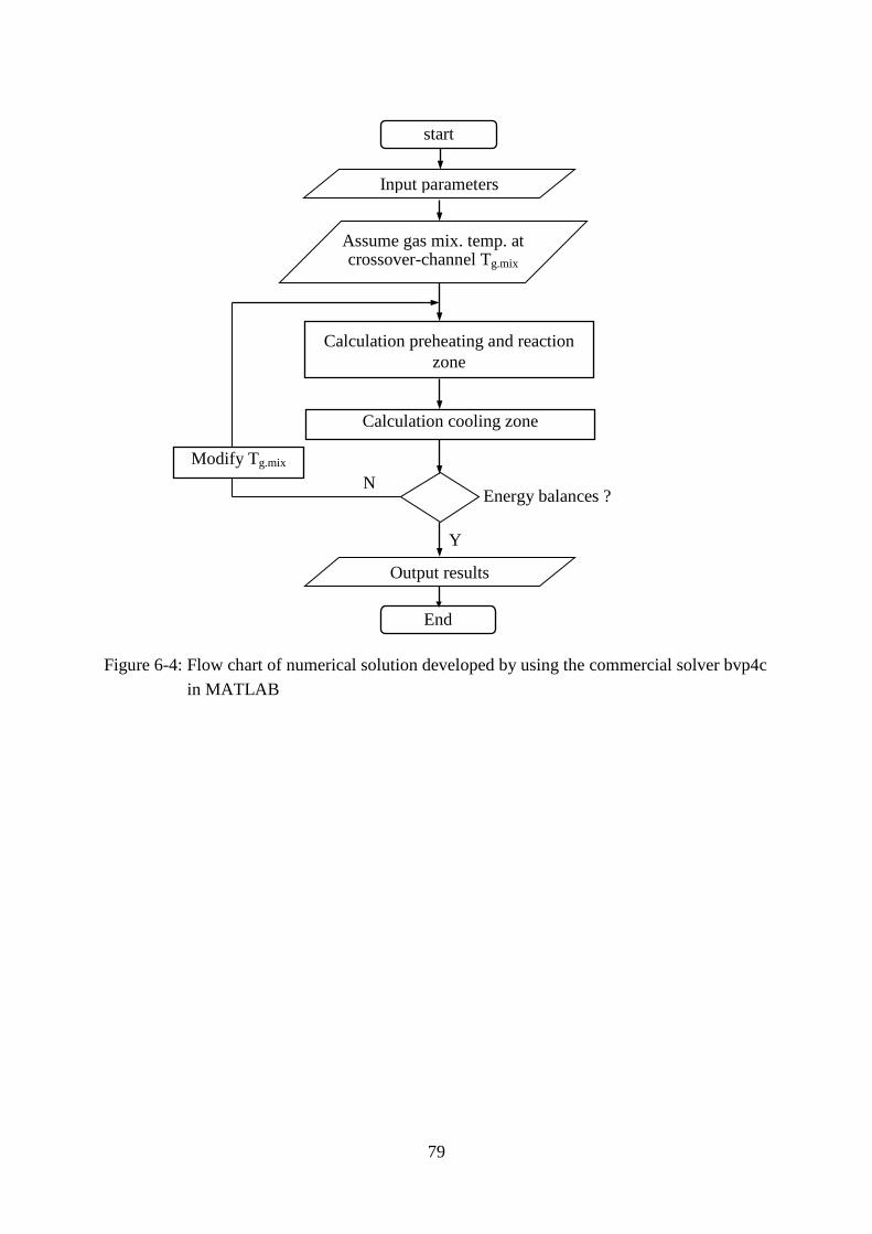
79

Figure 6-4: Flow chart of numerical solution developed by using the commercial solver bvp4c in MATLAB

flue gasin

start

Assume gas mix. temp. at crossover-channel Tg.mix

Calculation preheating and reaction zone

Input parameters

Energy balances ?

Y

Output results

N

End

Calculation cooling zone

Modify Tg.mix

80

6.3 Results of simulation

6.3.1 Basic input data Table 6-1 describes general input variables for simulations. The kiln (one shaft) has a total solid bed height of 17 m. The total specific throughput of two shafts is 44 t/d/m2 so that each shaft has a throughput of 22 t/d/m2. The fuel used is the natural gas with the specific energy consumption of 3.45 MJ/kglime and the excess air number of 1.15. The mean particle size is 60 mm and the limestone contains 96 % of calcium carbonate. Table 6-1 Basic data for simulation of the PFR kiln

Input variables Units Value

Kiln dimension (one shaft)

Total length of solid bed m 17

Length of preheating zone m 6

Length of burning zone m 6

Length of crossover-channel m 0.5

Length of cooling zone m 4.5

Combustion process Heat consumption (natural gas fuel)

MJ/kglime 3.45

kcal/kglime 825

Excess air number (combustion air) - 1.15

Kiln operating process

Limestone input flow t/d/m2 38

Lime output flow t/d/m2 22

Combustion air flow m3air/kglime 1.12

Lime cooling air flow m3air/kglime 0.7

Lance cooling air flow m3air/kglime 0.1

Transport air flow m3air/kglime 0

Fuel flow m3/kglime 0.1

Air feed temperature oC 20

Limestone feed temperature oC 20

Lime and limestone

Mean particle size mm 60

Average void fraction of solid bed - 0.38

CaCO3 content in limestone % mas 96

81

6.3.2 Principal temperature and conversion profile Figure 6-5 shows the principal temperature and conversion profiles in a PFR kiln. The figure is illustrated in the horizontal direction, which is transferred corresponding to the schematic diagram of the PFR shaft shown before. As mentioned before, the mathematical models simulate the mean values of the periodic fluctuations. Therefore, the temperature profiles shown in this figure represent the mean values of the solid, the gas and the flue gas temperatures in the periodic case. Initially, the limestone is charged into the kiln at the top (0 m) at an ambient temperature of 20°C. The stone is preheated by the flue gas in the non-burning mode with counter-current flow arrangement. After that, in the burning mode, it transfers heat to the combustion air characterized by co-current flow. The temperatures of both the stone and the combustion air increase in this zone. The firing zone begins at 6 m where the fuel is introduced through the lances. It is assumed that the combustion of the mixture of the fuel and the air starts immediately, thus the gas temperature starts increasing rapidly. The stone temperature also increases and it reaches the reaction temperature (820oC) at 6.3 m. The decomposition of the stone begins and its mass fraction starts decreasing. In the region from 6 m to 7 m, the solid temperature is lower than the flue gas temperature but it is still higher than the gas temperature. After that, because of higher combustion rate, the combustion gas temperature increases faster and it exceeds the solid temperature, thus both the combustion gas and the flue gas transfer heat to the solid. The solid temperature keeps increasing until it gets higher than the flue gas temperature at 8 m. As a result, from this position to the end of the firing zone (12 m), the solid gets heat from the combustion gas (in burning mode) and it transfers heat to the flue gas (in non-burning mode). The solid leaves the firing zone with a temperature of about 1010 oC then it enters the cooling zone where it is cooled down by the cooling air until it reaches the lime discharge temperature.

Table 6-2 Results of simulation of the PFR kiln

Outputs Unit Values

Flue gas temperature oC 103

Lime discharge temperature oC 82

Calcination length m 5.7

Residual CO2 % 1.9

Maximum gas temperature oC 1240

Maximum solid temperature oC 1068

Total pressure drop mbar 340

Heat loss by the kiln wall % 6.1

82

In addition, other characteristic values of the simulations are summarized in Table 6-2 in the same manner as before. The temperature of the flue gas is 103 oC and that of the lime discharge is 82 oC. The maximum temperature of the gas is 1240 °C and that of the solid is 1068 °C. The heat loss through the kiln wall is about 6.1 % and the pressure drop is 340 mbar.

Figure 6-5: Principal temperature and mass fraction profiles in a PFR kiln

An important remark is observed from the Figure 6-5 that the flue gas leaving the burning shaft is heated up in the non-burning shaft by the solid. At the kiln height of about 8 m, the

0

200

400

600

800

1000

1200

0 6 12

Tem

pera

ture

in o C

17

Tg

Tfg

Tsw

Ta Ta

flame

preheating burning cooling

Tsf

natural gas E=825 kcal/kglime 3.45 MJ/kglime mlime=22.0 t/d/m2

a)

.

1

1,2

1,4

1,6

1,8

2

2,2

0 6 12

Mas

s fra

ctio

n in

kg/

kglim

e

Axial position in m

calcination

17

solid

air

gas

non-burning shaft

air

b)

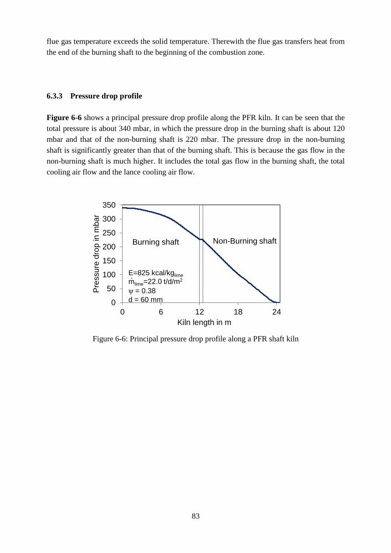
83

flue gas temperature exceeds the solid temperature. Therewith the flue gas transfers heat from the end of the burning shaft to the beginning of the combustion zone. 6.3.3 Pressure drop profile Figure 6-6 shows a principal pressure drop profile along the PFR kiln. It can be seen that the total pressure is about 340 mbar, in which the pressure drop in the burning shaft is about 120 mbar and that of the non-burning shaft is 220 mbar. The pressure drop in the non-burning shaft is significantly greater than that of the burning shaft. This is because the gas flow in the non-burning shaft is much higher. It includes the total gas flow in the burning shaft, the total cooling air flow and the lance cooling air flow.

Figure 6-6: Principal pressure drop profile along a PFR shaft kiln

0

50

100

150

200

250

300

350

0 6 12 18 24

Pre

ssur

e dr

op in

mba

r

Kiln length in m

Burning shaft Non-Burning shaft

E=825 kcal/kglime mlime=22.0 t/d/m2

ψ = 0.38 d = 60 mm

.

84

6.4 Influencing parameters

6.4.1 Influence of energy input Figure 6-7 shows the temperature and the conversion profiles in the burning zone for different energy inputs. As an example, simulations were done for the energy input varied in the range of 810 - 840 kcal/kglime and other inputs were kept the same as given in Table 6-1.

Table 6-3 Influences of energy input

Energy input kcal/kglime 810 825 840


Lime temperature oC 76 80 91

Residual CO2 % 2.6 1.9 1.3


Max.solid temperature oC 1036 1068 1130


As observed before in the normal shaft kiln, the higher the energy input, the more heat is generated by the combustion, this results in a higher kiln temperature. Hence, the decomposition process becomes faster and requires a shorter zone. In addition, Table 6-3 summarizes the characteristic values of the simulation. The flue gas, the lime discharge, the kiln maximum temperatures and the pressure drop increase with the increase of the energy. However, the residual CO2 decreases with the increase of the energy.

85

Figure 6-7: Influence of energy input on the temperature and the conversion profiles

700

800

900

1000

1100

1200

1300

6 8 10 12

Gas

tem

p., i

n o C

3 1. E=840 kcal/kglime 2. E=825 kcal/kglime 3. E=810 kcal/kglime

2

1

a)

700

800

900

1000

1100

1200

6 8 10 12

Sol

id s

ufac

e te

mp.

in o C

3

2

1

b)

mlime=22.0 t/d/m2 d=60 mm

.

1

1,2

1,4

1,6

1,8

6 8 10 12

Sol

id m

ass

fract

. in

kg/k

g lim

e

Burning zone length in m

3

2 1

c)

86

6.4.2 Influence of lime throughput Figure 6-8 and Table 6-4 show the simulation results in the same manner as before for different kiln throughputs. Simulations were done for the kiln throughput varied in the range of 20.5 – 23.5 t/d/m2 while other inputs were kept the same as given in Table 6-1. Similar to the normal shaft kiln, a lower kiln throughput leads to a longer residence time and causes a higher kiln temperature. This results in a faster calcination rate and a shorter calcination zone. In addition, in Table 6-4, it is observed again that the residual CO2 and the pressure drop increases considerably with an increase of the kiln throughput. However, the kiln maximum temperature decreases significantly.

Table 6-4 Influences of lime throughput

Lime throughput t/d/m2 20.5 22.0 23.5



Residual CO2 % 1.5 1.9 2.4




87

Figure 6-8: Influence of kiln throughput on the temperature and the conversion profiles

700

800

900

1000

1100

1200

1300

6 8 10 12

Gas

tem

pe.,

in o C

3 1. mlime=20.5 t/d/m2 2. mlime=22.0 t/d/m2 3. mlime=23.5 t/d/m2

2

1

a)

.

.

.

700

800

900

1000

1100

1200

6 8 10 12

Sol

id s

urfa

ce te

mp.

in o C

3 E= 825 kcal/kglime d=60 mm

2

1

b)

1

1,2

1,4

1,6

1,8

6 8 10 12

Sol

id m

ass

fract

. in

kg/k

g lim

e


3 2

1

c)

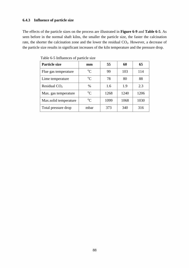
88

6.4.3 Influence of particle size The effects of the particle sizes on the process are illustrated in Figure 6-9 and Table 6-5. As seen before in the normal shaft kilns, the smaller the particle size, the faster the calcination rate, the shorter the calcination zone and the lower the residual CO2. However, a decrease of the particle size results in significant increases of the kiln temperature and the pressure drop.

Table 6-5 Influences of particle size

Particle size mm 55 60 65



Residual CO2 % 1.6 1.9 2.3




89

Figure 6-9: Influence of particle size on the temperature and the conversion profiles

700

800

900

1000

1100

1200

1300

6 8 10 12

Gas

tem

pe.,

in o C

3 1. d=55 mm

2. d=60 mm 3. d=65 mm

2

1

a)

700

800

900

1000

1100

1200

6 8 10 12

Sol

id s

urfa

ce te

mp.

in o C

3

2

1

b)

mlime=22.0 t/d/m2

E= 825 kcal/kglime .

1

1,2

1,4

1,6

1,8

6 8 10 12

Sol

id m

ass

fract

., in

kg/

kglim

e


1

2

3

c)

90

6.4.4 Influence of limestone origin As mentioned before, limestones of different origins differ in their properties such as the reaction coefficient and the thermal conductivity. As the first example, two types of limestones with different thermal conductivity were selected for simulations. The simulation results are shown in Figure 6-10 and Table 6-6.

Table 6-6 Influences of thermal conductivity

Limestone No.1

(λ=0.6 W/m/K) No.2

(λ=0.8 W/m/K) Flue gas temperature oC 115 99

Lime temperature oC 93 78

Residual CO2 % 2.3 1.5


Max. solid surface temp. oC 1092 1081

Average solid core temp. oC 870 890

Total pressure drop mbar 334 338

In Figure 6-10, the surface and the core temperatures of the solid particles are plotted together to compare. The limestone No.2 with a higher thermal conductivity decomposes faster, needs a shorter calcination zone and results in a lower residual CO2. The limestone with a higher thermal conductivity needs a lower temperature difference between the surface and the core as driving force for the decomposition process. Therefore, this causes a higher core temperature and a lower surface temperature, while the average temperature of the lime layer will stay roughly the same. Figure 6-11 and Table 6-7 show the simulation results for limestones with different reaction coefficients. According to Cheng et al. [56, 57], the reaction coefficient varies in the range from 0.004 to 0.012 m/s within a factor of 3. As an example, simulations were done by using the lowest and the highest values of the reaction coefficient. It can be seen that a higher reaction coefficient leads to a faster decomposition rate and a shorter calcination zone, thus it results in a lower residual CO2. In addition, a larger reaction coefficient needs a lower decomposition pressure as driving force and thus a lower reaction front temperature. Besides, a larger reaction coefficient leads to a lower average temperature of the lime layer. This is not the case with the thermal conductivity since the average temperature of the lime layer stays roughly the same. 58

91

Figure 6-10: Influence of thermal conductivity on the temperature and conversion profiles

700

800

900

1000

1100

1200

6 8 10 12

Gas

tem

pe.,

in o C

a)

λ1= 0.6 W/K/m λ2= 0.8 W/K/m

700

800

900

1000

1100

1200

6 8 10 12

Sol

id te

mp.

in o C

Tsw1

Tsw2

Tsf2

Tsf1

λ1 λ2

b)

1

1,2

1,4

1,6

1,8

6 8 10 12

Sol

id m

ass

fract

. in

kg/k

g lim

e


λ1 λ2

c)

mlime=22.0 t/d/m2

E= 825 kcal/kglime d=60 mm

.

92

Figure 6-11: Influence of reaction coefficient on the temperature and conversion profiles

700

800

900

1000

1100

1200

6 8 10 12

Gas

tem

pera

ture

in o C

a)

k1=0.004 m/s k2=0.012 m/s

700

800

900

1000

1100

1200

6 8 10 12

Sol

id te

mp.

in o C

Tsw2 Tsw1

Tsf1

Tsf2

k1 k2

b)

1

1,2

1,4

1,6

1,8

6 8 10 12

Sol

id m

ass

fract

. in

kg/k

g lim

e


k1 k2

c)

mlime=22.0 t/d/m2

E= 825 kcal/kglime d=60 mm

.

93

Table 6-7 Influences of the reaction coefficient

Limestone No.3

(k=0.004 m/s) No.4

(k=0.012 m/s) Flue gas temperature oC 118 86

Lime discharge temp. oC 100 70


Max. gas temperature

oC 1224 1231

Max. solid surface temp oC 1088 1078

Average solid core tempe oC 920 840


6.4.5 Influence of excess air number Figure 6-12 and Table 6-8 reveal the simulation results for different excess air numbers. Simulations were done for the excess air numbers varied in the range from 1.05 to 1.2 while other inputs were kept the same as before. Similar to the normal shaft kilns, it can be seen again that an increase of the excess air number results in a lower kiln temperature, but it leads to a higher residual CO2 and a higher pressure drop.

Table 6-8 Influences of excess air number

Eff. excess air number - 1.05 1.15 1.20



Residual CO2 % 1.6 1.9 2.2




94

Figure 6-12: Influence of excess air number on temperature and the conversion profiles

700

800

900

1000

1100

1200

1300

6 8 10 12

Gas

tem

pe.,

in o C

3 1. λf= 1.05

2. λf= 1.15 3. λf= 1.20

2

1

a)

700

800

900

1000

1100

1200

6 8 10 12

Sol

id s

urfa

ce te

mp.

in o C

3 mlime=22.0 t/d/m2 E= 825 kcal/kglime d= 60 mm

2

1

b)

.

1

1,2

1,4

1,6

1,8

6 8 10 12

Sol

id m

ass

fract

. in

kg/k

g lim

e


3 2

1

c)

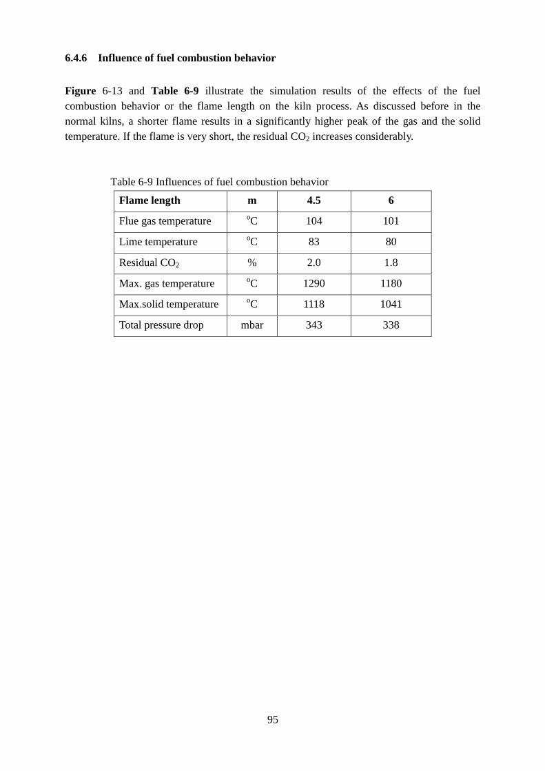
95

6.4.6 Influence of fuel combustion behavior Figure 6-13 and Table 6-9 illustrate the simulation results of the effects of the fuel combustion behavior or the flame length on the kiln process. As discussed before in the normal kilns, a shorter flame results in a significantly higher peak of the gas and the solid temperature. If the flame is very short, the residual CO2 increases considerably.

Table 6-9 Influences of fuel combustion behavior

Flame length m 4.5 6

Flue gas temperature oC 104 101

Lime temperature oC 83 80



Max.solid temperature oC 1118 1041


96

Figure 6-13: Influences of fuel combustion behavior on the temperature profiles

0

20

40

60

80

100

6 7 8 9 10 11 12

Fuel

con

vers

ion

in %

1. short flame 2. long flame

a)

2 1

700

800

900

1000

1100

1200

1300

6 7 8 9 10 11 12

Gas

tem

p. in

o C

b)


d=60 mm

.

700

800

900

1000

1100

1200

6 7 8 9 10 11 12

Sol

id s

urfa

ce te

mp.

in o

C


1

2

c)

97

6.5 Influence of kiln dimension Finally, the influence of the lengths of the preheating, the firing and the cooling zones on the process is investigated. As an example, Figure 6-14 shows the simulations results for the first case with different preheating zone lengths of 6 m and 4 m. It can be seen that a shorter preheating zone results in a lower kiln temperature, but it leads to a higher residual CO2, Table 6-10. In this simulation, by shortening the preheating zone by 2 m, the residual CO2 increases from 1.9 % to 2.3 %. In the second simulation, the firing zone is extended from 6 m to 8 m. This extension of the firing zone results in a decrease of the residual CO2 from 2.3 % to 1.8 %. However, it also leads to considerable increases of the kiln maximum temperatures and the pressure drop.

Table 6-10 Influences of the kiln length

Case Ref. 1 2

Preheating zone length m 6 4 4

Firing zone length m 6 6 8



Residual CO2 % 1.9 2.3 1.8




Figure 6-15 illustrates the simulation results for different cooling zone lengths. Simulations were done in two cases for the cooling zone lengths of 4 m and 5 m. To see how the cooling length affects the cooling process, it is assumed in both cases that the lime enters the cooling zone with the same temperature of 1000oC. A shorter cooling zone results in a faster cooling lime process, however it leads to a higher lime discharge temperature, Table 6-11. In this simulation, by shortening the cooling zone by 1 m, the lime discharge temperature increases almost 12 oC. The lime discharge temperature can be lowered by introducing more cooling air. For example, in Table 6-11 it shows that the lime discharge temperature decreases 14 oC by increasing the cooling air from 0.7 to 0.72 m3

air/kglime. 5960616263

Table 6-11 Influences of the cooling zone length

98

Cooling zone length m 5 4 4

Cooling air factor m3air/kglime 0.7 0.7 0.72

Tlime.in oC 1000 1000 1000

Tair.in oC 20 20 20

Tlime.out oC 80 92 78

Figure 6-14: Influence of the length of preheating zone on the temperature profiles

0

200

400

600

800

1000

1200

0 3 6 9 12 15

Tem

pera

ture

in o C

Kiln length in m

1. preheating zone, 6m 2. preheating zone, 4m

4m pre.,

6m preheating


Tg1

Ts1 Tg2

Ts2

.

99

Figure 6-15: Influence of the length of cooling zone on the temperature profiles

0

200

400

600

800

1000

0 1 2 3 4 5

Tem

pera

ture

in o C

Cooling zone length in m

1. cooling zone, 5m 2. cooling zone, 4m

γac=0.70 m3air/kglime

d= 60 mm mlime= 22.0 t/d/m2

Ts1

Ts2

Ta1 Ta2

.

100

7 Measurement and validation of temperature profile 7.1 Normal shaft kilns Two normal shaft kilns were selected for the measurement. Figure 7-1 shows a schematic diagram of the chosen normal shaft kiln A. The kiln has a total solid bed height of 12 m, in which the height from the top to the burner level is about 7.5 m. The level 0 m is defined as an average value of the filling level of stones at the kiln top. The kiln has a throughput of 200 t/d. Thermocouples (type K, Ni-Cr/Ni) with a length of 30 m, a diameter of 6 mm and a maximum permissible temperature of 1370 oC, were inserted from the top. During the measurement the thermocouple moved downward together with the stones. The values of the temperature were recorded electronically every 10 - 15 sec. The length of the thermocouple inserted into the solid bed at the top was also recorded. Prior to the experiment the kiln had been operating for several weeks with the same throughput so that the steady-state condition was ensured during the experiment.

Figure 7-1: Arrangements of measuring temperatures in normal shaft kiln

cool

ing

bu

rnin

g

pre

heat

ing

stone

air

fuel

lime

Depth

0 m

7.5 m

12 m

Thermocouple T2 T1

101

Figure 7-2: Kilns chosen for measuring temperatures

Figure 7-3: Inserting thermocouples during measurements

102

Figure 7-4 shows the measured temperatures in the normal shaft kiln A, in which two thermocouples T1 and T2 were inserted. The measured values are plotted in dependence on the depth of the solid bed, in which the coordinate 0 m represents the top of the solid bed. An assumption is that the thermocouples are supposed to move vertically with the solid bed, thus their position is considered the same as the solid bed depth. It can be seen that from the kiln top to about 4 m, both profiles reveal a similar behavior. However, after 4 m the two profiles are significantly different. The thermocouple T1 shows an increase of temperature while the thermocouple T2 remains at a relative constant temperature (830 oC) in a long range.

Figure 7-4: Measured temperatures in the normal shaft kiln A

Figure 7-5: Measured temperatures in the normal shaft kiln B The maximum temperature difference between the two profiles is almost 400 oC at about 5.5 m. There can be multiple reasons causing this difference: a) the condition in the normal shaft

0

200

400

600

800

1000

1200

1400

0 2 4 6 8

Tem

pera

ture

in o C

Distance from the top of solid bed in m

T1

T2

preheating reaction

fuel

T1 T2

600

800

1000

1200

1400

0 2 4 6 8

Tem

pera

ture

in °

C


preheating reaction

fuel

T2 T1

T3 T5 T4

103

kiln cross-section is not homogeneous; b) the actual positions of two thermocouples are not the same as shown in the figure; c) the thermocouple T1 moves directly to a burner while the thermocouple T2 is in between the burners. The maximum permissible temperature (1370 oC) of the thermocouples is reached at about 6 m, and then the two thermocouples fail before the fuel injection at about 7.5 m, thus the completed profiles could not be obtained. Figure 7-5 shows the measured temperatures in the normal shaft kiln B, which has a throughput of 180 t/d of lime. In this measurement, five thermocouples (T1 – T5) with a length of 20 m and a diameter of 3 mm were used. Due to some technical problems, the temperatures were recorded only after the thermocouples moved almost 1.5 m from the top of solid bed. It can be seen again that the five thermocouples show different behavior, especially after 6 m. The maximum temperature difference is also almost 400 oC. As mentioned before, this can be a result of inhomogeneous conditions in the cross-section of the kiln. Furthermore, the figure demonstrates again that all thermocouples fail after reaching the temperatures of 1370 oC. As a consequence, the temperatures in the burning zone, which are much higher than the permissible temperature of thermocouples type K, can not be measured. To measure the temperatures in the burning zone of the normal shaft kilns, special thermocouples such as Pt-Rh/Pt are required. However they are too expensive because of the long length (20 – 30 m) making simulations necessary. Mathematical model is used to simulate the temperature profiles in the normal shaft kiln kilns chosen for the measurements. Figure 7-6 shows the simulated profiles in the normal shaft kiln A, in which the results are compared with the temperatures measured by thermocouple T1 (Figure 7-4). A remark here is that the solid (surface) temperatures predicted by the model are close to the measured temperature. This can be expected due to two reasons: a) in a high temperature range, the heat transfer by radiation from the stones to the thermocouples is stronger than that by convection from the gas to the thermocouples; b) the thermocouples may be fixed or contacted with the stones during the measurement. As a result, the thermocouples measured mainly the solid surface temperature. In addition, it can be seen from the simulated profiles that the difference between the gas / flue gas and the solid temperatures is significant. The simulated profiles show a significant temperature difference between the gas and the solid. The maximum temperatures predicted by the model are about 1600 oC. The peak temperatures are in the regions near the burners. Unfortunately, it is not possible to compare the values and positions of the peak temperatures with the experiment. To compare positions of the peak temperature, measurements of the outer shell temperature were carried out and the results are presented in the following. Figure 7-7 shows the outer shell temperature profiles in the normal shaft kiln A. Temperatures at four different positions in circumferences were measured by an Infrared thermometer. It can be seen that shell temperatures have a maximum value of about 165 oC. The maximum values distribute at a position of about 6.0 m. A remark here is that this position is in the range of the maximum temperatures predicted by the model and shown before in Figure 7-6.

104

Figure 7-6: Measured & simulated temperatures in the RCE-kiln A

Figure 7-7: Outer shell temperatures in the normal shaft kiln A

Figure 7-8 shows the simulated temperature profiles in the normal shaft kiln B. The results are compared with the temperature profiles measured by the two thermocouples T3 and T4 (Figure 7-5). It can be seen again that the measured temperatures are similar to the lime surface temperature calculated by the model. The maximum temperatures are about 1500 oC

0

400

800

1200

1600

0 2 4 6 8 10 12

Tem

pera

ture

in o C

Distance from the top of solid bed


Tgas

Tsolid

Tmeasured

lignite fuel throughput: 200 t/d

0

30

60

90

120

150

180

0 2 4 6 8 10 12

She

ll te

mpe

ratu

re in

o C


cross-section

measured


simulated

105

and they distribute near the burners. Unfortunately, there is no measured shell temperature profile, thus the position of the peak temperatures inside the kiln is not possible to validate.

Figure 7-8: Measured & simulated temperatures in the normal shaft kiln B

0

400

800

1200

1600

0 2 4 6 8

Tem

pera

ture

in °

C


Tgas

Tsolid

lignite fuel throughput: 180 t/d

Tmeasured

preheating reaction

106

7.2 PFR kilns The procedure for measuring the temperature profiles in the PFR kiln is similar to that of the normal shaft kilns kiln. The kiln has a total solid bed height of 18 m, in which the height from the top to the cross-over channel is 14 m. The kiln has a total throughput of 370 t/d. In each shaft (S1, S2) of the kiln, a thermocouple type K, which has the same specification as mentioned before (used for normal shaft kiln A) was inserted from the top. Figure 7-9 shows the temperatures measured in two shafts S1 and S2 of the PFR kiln. It can be seen that at the beginning of the preheating zone both profiles fluctuate with changes of about 50 - 100 oC, then the changes become higher. Temperatures can even be up to 300 oC in the burning zone. This is due to the fact that two shafts are operated in two distinct modes, burning and non-burning with a periodic time of about 14 min for each cycle. From 0 m to 4 m the two profiles show similar behaviors. However, after 4 m there is a significant temperature difference between the two profiles. The thermocouple in shaft S1 seems to have a delay and the temperatures measured in shaft S1 are lower than that of shaft S2. For example, at about 6 m the temperature difference between the two shafts is almost 300 oC. There can be a number of reasons causing this difference. Firstly, the thermocouple in shaft S1 did not move vertically together with the stones, it may be shifted in the solid bed; thus its position is not as deep as the solid bed depth shown in the figure. Secondly, the thermocouple in shaft S2 may be directly below the burners (outlet of lances) while the thermocouple in shaft S1 is between the lances. Thirdly, it can be also that the length of lances is different since it is known that this length is shortened randomly with time. Finally, the last reason can be that the fuel supply through the lances is not homogeneous in the cross section of the PFR-kiln. Due to some technical problems, the measurement was stopped when one thermocouple arrived at the cross-over channel (14 m). Therefore, the temperature profiles in the cooling zone were not measured. However, these profiles are not important for the validation of the simulation. As mentioned before, the thermocouple in shaft S1 could be shifted in the solid bed during the measurement. Therefore, its length shown before in Figure 7-9 is shortened, for example by 2 m. Figure 7-10 shows the new modified temperature profile in shaft S1, in which the temperature profile in shaft S2 is also plotted. It can be seen that the two profiles are more similar. However, a temperature difference of about 100 oC is still observed between the two shafts, particularly in the burning zone. This difference can be caused by two reasons. Firstly, the operating conditions between the two shafts are different; however this seems to be improbable. Secondly, the cross-section has an inhomogeneous temperature distribution because of imperfect fuel distribution for example.

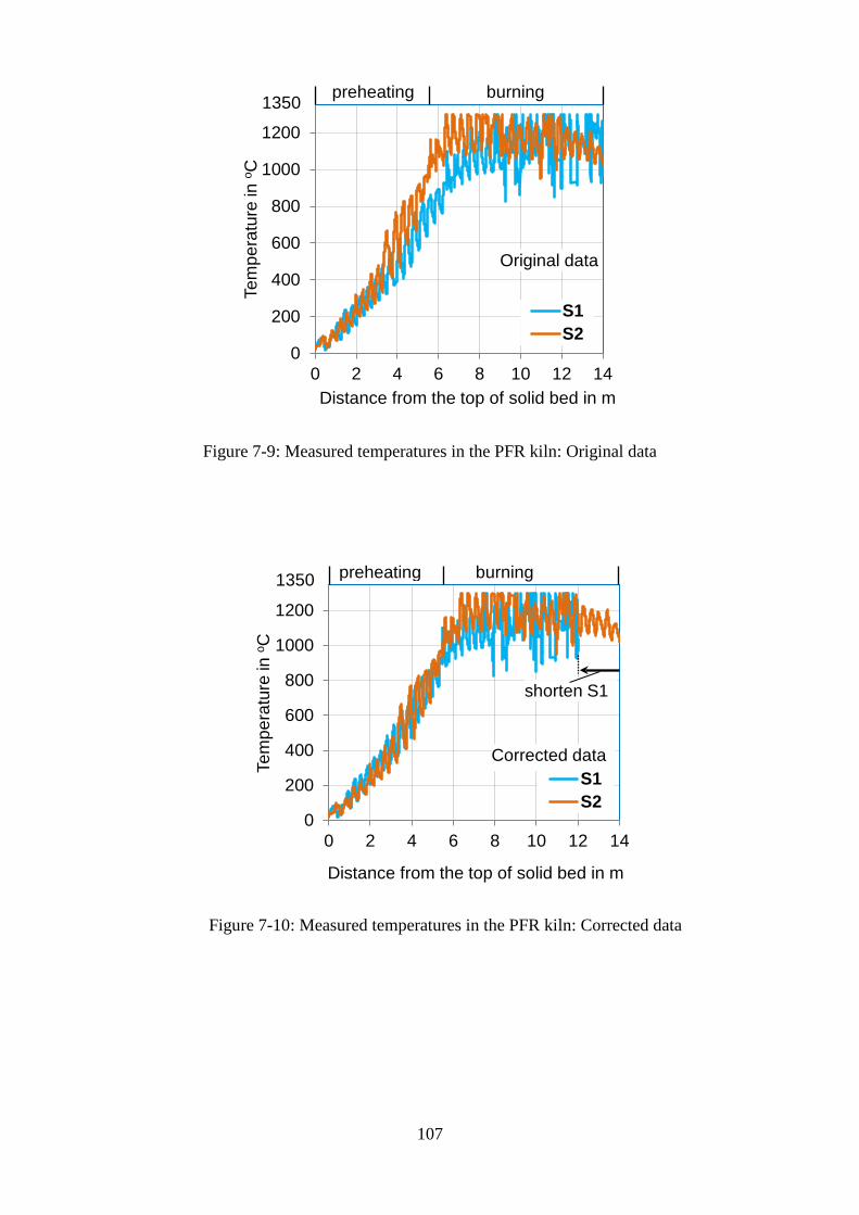
107

Figure 7-9: Measured temperatures in the PFR kiln: Original data

Figure 7-10: Measured temperatures in the PFR kiln: Corrected data

0

200

400

600

800

1000

1200

0 2 4 6 8 10 12 14

Tem

pera

ture

in o C


S1S2

Original data

preheating burning 1350

0

200

400

600

800

1000

1200

0 2 4 6 8 10 12 14

Tem

pera

ture

in o C


S1S2

Corrected data

1350 preheating burning

shorten S1

108

Figure 7-11: Measured & simulated temperatures in the PFR kiln

Figure 7-12: Outer shell temperatures in the PFR kiln

0

200

400

600

800

1000

1200

0 3 6 9 12 15 18

Tem

pera

ture

in o C


Tmeasured

Tair/Tgas Tsolid Tf.gas

natural gas & lignite fuel throughput: 370 t/d

preheating burning cooling 1350

0

20

40

60

80

0 3 6 9 12 15 18

She

ll te

mp.

, in

o C


preheating burning cooling

wind

measured

simulated

109

The mathematical model is used to simulate the temperature profiles in the PFR kiln. Figure 7-11 shows the simulated profiles, which are compared with the temperatures measured in shaft S2. As mentioned before, the model is used to calculate the mean values of the periodic fluctuations. Therefore, in Figure 7-11, the calculated profiles represent the mean temperature values of the gas, the flue gas and the solid (limestone / lime). It can be seen that the simulated values lie in the range of the measurement. It can be seen that the solid (surface) temperatures predicted by the model are close to the average values of the measurement. The reason is explained as before with the normal shaft kilns. In addition, it can be seen from the simulated profiles that the difference between the gas / flue gas and the solid temperatures is significant, particularly in the burning zone. The difference can be up to 100 oC at the beginning of this zone then it decreases reaching the end of this zone. As discussed before, it is not possible to observe this temperature difference by the measurement. Figure 7-12 shows the outer shell temperatures along the PFR-kiln axis. It can be seen that the temperatures measured in a circumference are significantly different because they are affected by the wind direction. The temperatures measured on the side with the stagnation points of the wind direction are lower than that of the other sides because at the stagnation points the convective heat transfer coefficient is highest. Furthermore, it can be seen that the simulated profile lies in the range of the measured values. This profile shows a similar behavior to that of the simulated temperatures shown before in Figure 7-11.

110

8 Conclusions and outlook Conclusions One-dimensional mathematical models have been developed to simulate the lime burning process in the normal shaft kilns and the PFR kilns. The following significant outputs were determined:

• The solid core and surface temperatures of the lime / limestone particles

• The gas temperature, including the flue gas temperature

• The lime conversion degree or the residual CO2 in lime

• The heat loss by the kiln wall

• The pressure drop along the kiln axis

The models were used to investigate the parameters, which affect significantly the kiln process. The following essential information has been obtained:

• The increase of the energy input leads to the decrease of the residual CO2, but it causes the increase of the kiln temperatures as well as the pressure drop

• The decrease of the kiln throughput results in the decrease of the residual CO2 and the pressure drop; however, the kiln temperatures increase

• The smaller the particle size, the faster the burning process and the lower the residual CO2. However, a small particle size leads to a significant increase of the pressure drop

• A higher excess air number results in a lower kiln temperature, but it leads to a higher residual CO2 and a higher pressure drop

• Limestone with a low thermal conductivity or a low reaction coefficient causes a low calcination rate and requires a long calcination zone. Additionally, a lower reaction coefficient also results in a higher average temperature of the lime.

• The shorter the flame length, the higher the kiln maximum temperatures, but a short flame may cause a considerable increase of the residual CO2.

• The increase of the kiln length leads to the decrease of the residual CO2, but it also causes the increases of the kiln temperature and the pressure drop

111

The simulation results can be directly used for the purpose of designing and regulating the shaft kilns. As an example, the following describes several possibilities for regulating kiln processes. a) If the desire is to reduce the residual CO2, it can be done in different ways:

• Increase the energy consumption • Decrease the kiln throughput • Extend the height of solid bed (increase the solid residence time)

b) If the desire is to increase the kiln throughput while the residual CO2 must be fixed, the

two following possibilities can be done:

• Increase the energy consumption • Extend the height of solid bed

c) If the desire is to lower the kiln temperatures, especially the lime temperature, it can be

implemented by: • Decreasing the energy consumption • Increasing the excess air number • Increasing the kiln throughput or decreasing the solid bed height

The simulation results were validated by the experiments with measuring temperatures in industrial kilns. The results of experiments and those of simulations are in good agreement. In addition, the simulation results demonstrate that the maximum temperatures of solid particles in the PFR kilns are significantly lower than that in the normal shaft kilns. In the PFR kilns, they vary in the range of 1000 – 1100 oC while in the normal shaft kilns they are in the range of 1400 – 1500 oC. Therefore, for producing soft-burnt lime, the PFR kilns are suitable whereas the normal shaft kilns are suitable for the production of hard-burnt lime. Outlooks

• Observations from experiments have shown that the condition at one cross-section along the kiln axis is inhomogeneous while it is assumed in the mathematical models (1D) of the present work as homogeneous. Further work should focus on this issue by developing 2D or 3D simulations.

• The mathematical models deal with only the spheres of the same size. Future works should be extended to particle size distribution and actual particle shapes.

112

• The fuel combustion is treated in a simple way with a given burning profile. It should be described as a function, which depends on the oxygen concentration, the excess air number, the types of fuel etc.

• With the PFR kilns, the mathematical models deal with the mean values of the periodic fluctuations. The actual periodic behaviors should be considered in future work.

113

Appendix The BVP Solver The function bvp4c solves two-point boundary value problems for ordinary differential equations (ODEs). It integrates a system of first-order ordinary differential equations,

)y,x(fy, = on the interval [a b] subject to general two-point boundary conditions,

0))b(y),a(y(bc = It can also accommodate other types of boundary value problems, such as those that have any of the following: • Unknown parameters • Singularities in the solutions • Multipoint conditions. In this case, the number of boundary conditions must be sufficient to determine the solution and the unknown parameters. bvp4c produces a solution that is continuous on [a b] and has a continuous first derivative there. bvp4c is a finite difference code that implements the 3-stage Lobatto IIIa formula. This is a collocation formula and the collocation polynomial provides a C1-continuous solution that is fourth-order accurate uniformly in the interval of integration. Mesh selection and error control are based on the residual of the continuous solution. The collocation technique uses a mesh of points to divide the interval of integration into subintervals. The solver determines a numerical solution by solving a global system of algebraic equations resulting from the boundary conditions, and the collocation conditions imposed on all the subintervals. The solver then estimates the error of the numerical solution on each subinterval. If the solution does not satisfy the tolerance criteria, the solver adapts the mesh and repeats the process. The user must provide the points of the initial mesh as well as an initial approximation of the solution at the mesh points.

114

References [1] Oates, J. A. H.. Lime and Limestone, Wiley- VCH, Weinheim, 1998. [2] Hills, A.W.D.: The mechanism of the thermal decomposition of calcium carbonate,

Chemical Engineering Science, Vol. 23, pp. 297–320, 1968. [3] Hisieh, C. L.: Evaluating the energy performance of a lime kiln, Tappi Journal, Vol. 66,

pp. 77- 79, 1983. [4] Zuideveld, P. L., Berg, P. J.: Design of lime shaft kiln, Chemical Engineering Science

Vol. 26, pp. 875-883, 1970. [5] Schwertmann, T.: Thermodynamic aspects of the counterflow lime burning process

(Part 1), Cement Lime Gypsum, Vol. 57, pp. 48-58, 2004. [6] Schwertmann, T.: Thermodynamic aspects of the counterflow lime burning process

(Part 2), Cement Lime Gypsum Vol. 57, pp. 64-67, 2004. [7] Piringer, H.: Fuel gases with low calorific value for firing PFR lime shaft kilns, Cement

Lime Gypsum, Vol. 56, pp. 66 - 72, 2003. [8] Lucian, P.: Lime production - The vertical process, Pit and Quarry Journal, Vol. 81, pp.

34 – 38, 1998. [9] Lang, G., Bao, C., Gao, S., Logan, R.L., Li, Y.: Study on the energy-saving technology

of Chinese shaft calciners, The Minerals, Metals & Materials Society, Wiley- VCH 2011.

[10] Sagapov, V. Sh., Burkin, M. V.: Theoretical modeling of simultaneous processes of coke burning and limestone decomposition in a furnace, Combustion Explosion Shock, Vol.44, No.1, pp. 55-63, 2008.

[11] YI-Zheng-ming, ZHOU Jie-min, CHEN Hong-rong.: Numerical simulation of thermal process and energy saving of lime furnace, Journal of Central South University of Technology, Vol. 12, pp. 295-299, 2005.

[12] Senegacnik, A., Oman, J., Brane, S.: Analysis calcination parameter and temperature profile in an annular shaft kiln. Part 1: Theoretical survey, Applied Thermal Engineering, Vol. 27, pp. 1467-1472, 2007.

[13] Senegacnik, A., Oman, J., Brane, S.: Analysis calcination parameter and temperature profile in an annular shaft kiln. Part 2: Results of test, Applied Thermal Engineering, Vol. 27, pp. 1473-1482, 2007.

[14] Drenhaus, T.B., Simsek, E., Scherer, V.: A couple fluid dynamic-discrete element simulation of heat and mass transfer in a lime shaft kiln, Chemical Engineering Science Vol. 65, pp. 2821-2834, 2010.

[15] Canadian Minerals Yearbook for Lime, 1998. [16] U.S. Geological Survey, Minerals Yearbook, 1999. [17] U.S. Geological Survey, Mineral Commodity Summaries,

http://minerals.usgs.gov/minerals/pubs/commodity/lime, February 2000. [18] U.S. Geological Survey, Mineral Commodity Summaries,

http://minerals.usgs.gov/minerals/pubs/commodity/lime, February 2009. [19] U.S. Geological Survey, Mineral Commodity Summaries,

http://minerals.usgs.gov/minerals/pubs/commodity/lime, February 2010. [20] European Commission: Reference Document on Best Available Techniques in the

Cement and Lime Manufacturing Industries, March 2010.

http://www.scopus.com/authid/detail.url?authorId=24399276300&eid=2-s2.0-79955129711





http://minerals.usgs.gov/minerals/pubs/commodity/lime



115

[21] Jenkins, B.: What are shaft kilns for lime manufacturers, IFRF online combustion

handbook, ISSN 1607-9116, 2003. [22] Ebertsch, G., Plickert, S.: German contribution to the BREF-Review, Part I: Lime

manufacturing industry, 2006. [23] Characteristics of some types of shaft kilns, http://www.ineris.fr.org/aida, 2007. [24] Lime market research in Russia and Central Federal District, http://www.infomine.ru,

2007. [25] Jeschar, R.: Heat transfer in pelletizing with mixed feed, Archiv für das

Eisenhüttenwesen, 35, H.6, 1964. [26] Jeschar, R., Specht, E., Alt, R.: Grundlagen der Wärmeübertragung. Viola-Jeschar-

Verlag, Goslar,1990. [27] Bes, A.: Dynamic Process simulation of limestone calcination in normal shaft kilns,

Dissertation, Otto-von-Guericke University Magdeburg, 2006. [28] Mills, A. F., Anthony, F., Basic heat and mass transfer, Prentice Hall, 1999. [29] Specht, E.: Kinetik der Abbaureaktionen, Cuvillier Verlag, Göttingen, 1993. [30] Furnas, C. C.: Flow of gases through beds of broken solids, Bull. 307, U.S. Bureau of

Mines, 1929. [31] Tsotsas, E.: VDI Wärmeatlas, Wärmeleitung und dispersion in durchströmten

Schütungen, 9. Auflage, 2002. [32] Giese, M.: Stromüng in porösen Medien unter Berücksichtigung efficktiver

Viskositäten, Dissertation, TU Müchen, 1998. [33] Ergun, S.: Fluid flow through packed columns, Chemical Engineering Process, Vol.48,

pp. 89-94, 1952. [34] Brauer, M.: Grundlagen der Einphasen- und Mehrphasenströmungen, Sauerländer

Verlag, Goslar, 1990. [35] Cheng, C.: Thermal processes simulation of reactive particles on moving grate,

Dissertation, Otto-von-Guericke University Magdeburg, 2007. [36] Shwertmann, T.: Untersuchung des Optimierungspotentials des Ringschachtofens

zum Brennen von carbonatischem Gestein, Dissertation, Otto-von-Guericke University Magdeburg, 2007.

[37] Szekely, J., Evans , J.W, Sohn, H.Y.: Gas-Solid-Reactions, Academic press, New York, 1976.

[38] Kainer, H., Specht, E., Jeschar, R.: Die Porendifussions-, Reactions- und Wärmeleitkoeffizienten verschiedener Kalksteine und ihr Einfluss auf die

Zersetzungszeit, Cement Lime Gypsum, Vol. 39, pp. 214-219, 1986. [39] Silva, M., Specht, E., Schmidt, J.. Thermophysical properties of the limestone as a

function of origin (Part 2), Calcination enthalpy and equilibrium temperature, Cement Lime Gypsum 6, pp. 51-57, 2010.

[40] Bes, A., Specht, E., Kehse G.: Influence of the type of fuel on the energy consumption in lime burning, Cement Lime Gypsum, Vol.60, pp. 84-93, 2007.

[41] Chai, L., Navrotsky, A.: Thermochemistry of carbonate-pyroxene equilibrium, Contribution to Mineralogy and Petrology, Vol.114, pp. 139-147, 1993.

[42] Specht, E.: Combustion Technology, handout for Master of Safety, Quality and Environment, Otto-von-Guericke University Magdeburg.

http://www.ineris.fr.org/aida

http://www.infomine.ru/

116

[43] Collarini: Innovative design of high capacity twin shaft regenerative lime kilns, Cement

International Journal, Vol.7(3), pp. 38 – 42, 2009. [44] Piringer, H., Werner, W.: Process optimization on Maerz lime kilns, Cement Lime

Gypsum, Vol. 58, pp. 41-58, 2005. [45] Verma, C. L.: Simulation of lime shaft kilns using mathematical modeling, Cement

Lime Gypsum, Vol.12, pp. 576-582, 1990. [46] Verma, C. L., Dave, N.G., Saraf, S.K.: Performance estimation vis-à-vis design of

mixed-feed lime shaft kiln, Cement Lime Gypsum, Vol.9, pp 471-477, 1988. [47] Unaspekov, B. A., Strekalova, L. V.: A model study of the performance of a

Kazogneupor shaft kiln, Journal of Refractories and Industrial Ceramic, Vol. 48, No. 7-8, pp. 275-276, 2002.

[48] Sagapov, V. Sh., Burkin, M. V., A. V. Voromin, A. A. Shatov.: Calculation of limestone burning in coke-fired kiln, Theoretical Fundamental of Chemical Engineering, Vol. 38, No.4, pp. 441-447, 2004.

[49] Marias, F., Bruyeres, B.: Modelling of a biomass fired furnace for production of lime, Chemical Engineering Science, Vol. 64, pp. 3417-3426, 2009.

[50] Sheng-xiang, D., Qing-song, X., Zhie-min, Z.: A lime shaft kiln diagnostic expert system based on holographic monitoring and real-time simulation, Expert system with applications, Vol. 38, pp. 15400-15408, 2011.

[51] Hai Do, D., Specht, E.: Dynamic modeling of lime burning process in normal shaft kiln, Proceeding of Chemical Engineering Conference, CHEMECA2010, Adelaide Australia 2010, pp.3468-3478.

[52] Hai Do, D., Specht, E.: Numerical simulation of heat and mass transfer of limestone decomposition in normal shaft kiln, Proceeding of Thermal Engineering Joint Conference, ASME/JSME 8th USA 2011, pp. T10060 – T10060-10.

[53] Martins, M.A., Oliveira, L.S., Franca, A.S.: Modeling and simulation of limestone calcination in rotary kilns (part 2: industrial rotary kiln), Cement Lime Gypsum, Vol. 55, pp. 74–83, 2002.

[54] Senegacnik, A., Oman, J., Brane, S.: Influence of temperature profile in an annular shaft kiln on calcination, International Journal of Microstructure and Materials Properties, Vol. 1, No. 2, pp. 785-792, 2006.

[55] Manseung, L., Sihyung, L.: A mathematical model of calcination of limestone in rotary kiln, Journal of Steel Research, Vol. 70, pp. 15 - 21, 1999.

[56] Cheng, C., Specht, E.: Reaction coefficient in decomposition of lumpy limestone of different origin, Thermochimica acta, Vol. 449, pp. 8–15, 2006.

[57] Cheng, C., Specht, E., Kehse. G.: Influences of the origin and material properties of limestone on its decomposition behavior in shaft kilns, Cement Lime-Gypsum, Vol.60, pp. 51–61, 2007.

[58] Hai Do, D., Specht, E.: Determination of thermal conductivity, reaction coefficient and pore diffusivity in decomposition of limestone of different origin, Proceeding of the world congress on engineering and computer science, USA 2011, Vol. 2, pp.617-622.

[59] Bes, A., Specht, E., Kehse G.: Calculation of the cooling zone length and lime discharge temperature of lime shaft kilns, Cement Lime Gypsum, Vol. 60, pp. 63-73, 2007.

[60] HaiDo, D., Specht, E., Kehse, G., Ferri, V., Christiansen, T., L., Bresciani, P.: Simulation of lime calcination in PFR kiln – Influence of energy input and kiln throughput, Cement Lime Gypsum, Vol.12, pp.52- 64, 2011.

117

[61] HaiDo, D., Specht, E., Kehse, G., Ferri, V., Christiansen, T., L., Bresciani, P.:

Simulation of lime calcination in PFR kiln – Influence of source and size of limestone, Cement Lime Gypsum, Vol.4, pp.56- 65, 2012.

[62] Commandre, J.M., Salvado, S., Nzihou, A.: Reactivity of laboratory and industrial limes, Chemical Engineering Research and Design, Vol. 85, pp. 473-480, 2007.

[63] Kamperl, J., Maeck, J.: Precipitation of calcium carbonate from hydrated lime of variable reactivity, granulation and optical properties, International Journal of Mineral Process, Vol. 93, pp. 84-88, 2009.

Curriculum Vitae

Personal data Name: Duc Hai Do Date of Birth: March 15, 1979 Place of Birth: Vinh Phuc, VietNam Marital status: Married Nationality: VietNam Education 1994-1997 High school Vinh Yen High School, Vinh Phuc, VietNam 1997-2002 Bachelor of Chemical Engineering Major: Petrochemical – Organic Technology Hanoi University of Technology, Hanoi, VietNam 2006-2007 Master of Science Major: Quality, Safety and Environment (QSE)

Otto von Guericke University Magdeburg 2007-2012 Ph.D student Otto von Guericke University Magdeburg

Work experience Dec. 2002-Aug.2006 Process engineer, Chief operator

Dinh Co LPG and Refinery factory, PetroVietnam Gas Co., 101 Le Loi Str., Vung Tau, VietNam

Nov. 2007-Jun.2012 Scientific employee Otto von Guericke University Magdeburg

Awards 2002 The first prize in “Students’ Scientific Research” Award Ministry of Education and Training, VietNam 2002 Award for students with excellent graduation Hanoi University of Technology, VietNam 2006 Full DAAD scholarship for Master program Otto von Guericke University Magdeburg

Simulation of Lime Calcination in Normal Shaft and Parallel ...

Documents

Transcript of Simulation of Lime Calcination in Normal Shaft and Parallel ...