Ensaios Econômicos

Escola de

Pós-Graduação

em Economia

da Fundação

Getulio Vargas

N◦ 486 ISSN 0104-8910

Forecasting Electricity Demand Using Gener-

alized Long Memory

Lacir Jorge Soares, Leonardo Rocha Souza

Junho de 2003

URL: http://hdl.handle.net/10438/825

Os artigos publicados são de inteira responsabilidade de seus autores. Asopiniões neles emitidas não exprimem, necessariamente, o ponto de vista daFundação Getulio Vargas.

ESCOLA DE PÓS-GRADUAÇÃO EM ECONOMIA

Diretor Geral: Renato Fragelli CardosoDiretor de Ensino: Luis Henrique Bertolino BraidoDiretor de Pesquisa: João Victor IsslerDiretor de Publicações Cientí�cas: Ricardo de Oliveira Cavalcanti

Jorge Soares, Lacir

Forecasting Electricity Demand Using Generalized Long

Memory/ Lacir Jorge Soares, Leonardo Rocha Souza � Rio de

Janeiro : FGV,EPGE, 2010

(Ensaios Econômicos; 486)

Inclui bibliografia.

CDD-330

������� ���������� ��

� � � � � � � � � � � � � � � � � �� � � � � �� � � � �� � � � � � � �� � � � �� � � � �

� � � � �� � � �� � � ��

� � � � � � �� � � � � �� � � � �

�����������

Forecasting Electr icity Demand Using Generalized Long Memory

Lacir Jorge Soares

Department of Electrical Engineering

Catholic University of Rio de Janeiro

Leonardo Rocha Souza

Graduate School of Economics

Fundação Getúlio Vargas

June 2003

Abstract. This paper studies the electricity hourly load demand in the area covered by a

utility situated in the southeast of Brazil. We propose a stochastic model which employs

generalized long memory (by means of Gegenbauer processes) to model the seasonal

behavior of the load. The model is proposed for sectional data, that is, each hour’s load

is studied separately as a single series. This approach avoids modeling the intricate

intra-day pattern (load profile) displayed by the load, which varies throughout days of

the week and seasons. The forecasting performance of the model is compared with a

SARIMA benchmark using the years of 1999 and 2000 as the out-of-sample. The model

clearly outperforms the benchmark. We conclude for general long memory in the series.

Keywords. Long Memory, Generalized Long Memory, Load Forecasting.

2

1 – Introduction

Managing electricity supply is a complex task. The system operator is responsible for

the hourly scheduling of the generators and aims foremost at balancing power

production and demand. After this requirement is satisfied, it aims at minimizing

production costs, including those of starting and stopping power generating devices,

taking into account technical restrictions of electricity centrals. Finally, there must

always be a production surplus, so that local failures do not affect dramatically the

whole system. It is relevant for electric systems optimization, thus, to develop a

scheduling algorithm for the hourly generation and transmission of electricity. Amongst

the main inputs to this algorithm are hourly load forecasts for different time horizons.

Electricity load forecasting is thus an important topic, since accurate forecasts can avoid

wasting energy and prevent system failure. The former when there is no need to

generate power above a certain level and the latter when normal operation is unable to

withstand a heavy load. The importance of good forecasts for the operation of electric

systems is exemplified by many works in Bunn and Farmer (1985) with the figure that a

1% increase in the forecasting error would cause an increase of £10 M in the operating

costs per year in the UK.

There is also a utility-level reason for producing good load forecasts. Nowadays

they are able to buy and sell energy in the specific market whether there is shortfalls or

excess of energy, respectively. Accurately forecasting the electricity load demand can

lead to better contracts. Among the most important time horizons for forecasting hourly

loads we can cite: one to 168 hours ahead. This paper deals with forecasts of load

demand one to seven days (24 – 168 hours) ahead for a Brazilian utility situated in the

southeast of the country.

The data in study cover the years from 1990 to 2000 and consist of hourly load

demands. We work with sectional data, treating each hour as different time series, so

that 24 different models are estimated, one for each hour of the day. All models,

however, have the same structure. Ramanathan et al. (1997) won a load forecasting

competition at Puget Sound Power and Light Company using models individually

tailored for each hour. They also cite the use of hour-by-hour models at the Virginia

Electric Power Company. However, our approach differs from theirs in various ways,

including that we use only sectional data in each model. Using hour-by-hour models

avoids modeling the daily load profile, which varies for different days of the week and

different parts of the year, increasing model complexity much more intensely than

3

allowing improvements in the forecast accuracy. Although temperature is an influential

variable to hourly loads, temperature records for the region in study are very hard to

obtain and we focus our work on univariate modeling.

Long memory in stationary processes has traditionally two alternative

definitions, one in the frequency-domain and the other in the time-domain. In the

frequency-domain, this feature implies that the spectrum is proportional to |λ|-2d as the

frequency λ approaches zero. In the time-domain, the autocorrelations decay

hyperbolically, instead of geometrically as in ARMA processes (ρk ~ C|k|1-2d as k → ∞,

where k is the lag and C is a constant). In both cases, d is the long memory parameter

and the above relationships characterize long memory and stationarity if d ∈ (0, 0.5).

Good reviews of long memory literature are found in Beran (1994) and Baillie (1996).

Hosking (1981) and Granger and Joyeux (1980) proposed at the same time the

fractional integration, which has no physical but only mathematical sense. It is

represented by a noninteger power of (1 – B), where B is the backward-shift operator

such that BX t = X t-1, and can generate long memory while still keeping the process

stationary. Generalized (seasonal) long memory can be generated by a noninteger power

of the filter (1 – 2γB + B2) and the periodicity is implicit in the choice of the parameter

γ. Gray, Zhang and Woodward (1989) call such processes as Gegenbauer process,

because they admit Gegenbauer polynomials in the MA(∞) representation. They explore

the properties of Gegenbauer and related processes, which present the generalized long

memory feature. The noninteger power of a finite polynomial filter is equivalent to an

infinite polynomial filter, which can be obtained by a Binomial expansion.

The time series modeling includes a stochastic trend, seasonal dummies to

model the weekly pattern and the influence of holydays. After filtering these features

from the log-transformed data, there remains a clear seasonal (annual) pattern.

Analyzing the autocorrelogram, a damped sinusoid is observed, consistent with a

general long memory (Gegenbauer) process. The forecasting performance 24 to 168

hours ahead for the years 1999 and 2000 (each year separately) is compared with that of

a benchmark, namely a SARIMA model, and the results are highly favorable to our

modeling. For one day (24 hours) ahead, the model yields mean absolute percentage

error (MAPE) going from 2.2% (21th hour, 1999) to 4.4% (2nd hour, 2000), and for

seven days (168 hours) ahead it goes from 3.1% (20th hour, 1999) to 8.4% (3nd hour,

2000). Given the characteristics observed in the data and the results obtained in

4

forecasting, we conclude for the presence of generalized long memory in the data

studied.

The plan of the paper is as follows. The next Section briefly explains ordinary

and generalized long memory, both used in the modeling process. Section 3 describes

the data and the model proposed to fit the load demand, while Section 4 shows the

forecasting results of this modeling. Section 5 offers some concluding remarks.

2 – (Generalized) Long Memory

2.1 – Ordinary Long Memory

Stationary long memory processes are defined by the behavior of the spectral density

function near the frequency zero, as follows. Let f(λ) be the spectral density function of

the stationary process X t. If there exists a positive function )(cf λ , ],( ππλ −∈ , which

varies slowly as λ tends to zero, such that d ∈ (0, 0.5) and

0 as )(~)(2 →− λλλλ d

fcf , (1)

then X t is a stationary process with long memory with (long-)memory parameter d.

Alternatively, let ( )kρ be the k-th order autocorrelation of the series Xt. If there exists a

real number d ∈ (0, 0.5) and a positive function ( )c kρ slowly varying as k tends to

infinity, such that:

2 1( ) ~ ( ) as kdk c k kρρ − → ∞ (2)

then Xt is said to have long memory or long range dependence.

Xt is said to follow an ARFIMA(p,d,q) model if Φ Θ( )( ) ( )B B X Bdt t1− = ε ,

where εt is a mean-zero, constant variance white noise process, B is the backward shift

operator such that BXt = Xt-1, d is not restricted to integer values as in the ARIMA

specification, and Φ(B)= 1-φ1B-…-φpBp and Θ(B)=1+θ1B+…+θqB

q are the

autoregressive and moving-average polynomials, respectively. ARFIMA processes are

stationary and display long memory if the roots of Φ(B) are outside the unit circle and d

∈ (0, 0.5). If d < 0 the process is short memory and said to be “antipersistent”

(Mandelbrot, 1977, p.232), and Equation (1) holds so that the spectrum has a zero at the

zero frequency. Note that in this case the process does not fit into the definition of long

memory, since the parameter d is outside the range imposed by this definition. If d = 0

the ARFIMA process reduces itself to an ARMA. If the roots of Φ(B) are outside the

unit circle and d < 0.5, the process is stationary and if the roots of Θ(B) are outside the

5

unity circle and d > -0.5, the process is invertible. The autocorrelations of an ARFIMA

process follow ρ(k) ~ Ck2d-1 as the lag k tends to infinity and its spectral function

behaves as f(λ) ~ C|λ|-2d as λ tends to zero, satisfying thus (1) and (2). A non-integer

difference can be expanded into an infinite autoregressive or moving average

polynomial using the binomial theorem:

�∞

=−��

�

����

�=−

0

)()1(k

kd Bk

dB , (3)

where )1()1(

)1(

+−Γ+Γ+Γ=��

�

����

�

kdk

d

k

d and Γ(.) is the gamma function.

2.2 – Generalized Long Memory

Seasonal long memory is usually not defined in the literature, as different spectral

behaviors bear analogies with the definition in (1) within a seasonal context. Rather,

processes with these analogous properties are defined and their spectral and

autocovariance behaviors explored. We in this paper work with Gegenbauer processes

as in Gray, Zhang and Woodward (1989) and Chung (1996), but alternative models

have been used by Porter-Hudak (1990), Ray (1993) and Arteche (2002), for example.

The Gegenbauer processes were suggested by Hosking (1981) and later formalized by

Gray, Zhang and Woodward (1989) and are defined as follows. Consider the following

process

( ) tt

dXBB ε=+− 2�21 , (4)

where |γ| ≤ 1 and εt is a white noise. This process is called a Gegenbauer process,

because the Wold representation of (4) admits the important class of orthogonal

polynomials called Gegenbauer polynomials as the coefficients (Gray et al., 1989). This

Wold representation is achieved by using the binomial theorem as in (3), expanding the

representation to an MA(∞). If |γ| < 1 and 0 < d < ½, the autocorrelations of the process

defined in (4) can be approximated by

∞→= − k as )cos()( 12dkkCk νρ (5)

where C is a constant not depending on k (but depends on d and ν) and ν = cos-1(γ).

That means that the autocorrelations behave as a damped sinusoid of frequency ν and

that γ determines the period of the cycle (or seasonality). Moreover, the spectral density

function obeys

6

{ } df

22

coscos22

)(−−= νλ

πσλ (6)

behaving as λ → ν like

df

222~)(−

−νλλ (7)

for 0 ≤ λ ≤ π. Note that if γ = 1 then (4) is an FI(2d), or ARFIMA(0,2d,0), and that is

why we can call these processes as having the “generalized” long memory property.

Moreover, the (long memory) analogy of Gegenbauer processes with FI processes

comes from the fact that the latter have a pole or zero at the zero frequency while the

former have a pole or zero at the frequency ν, depending on whether d is respectively

positive or negative. Note that the Gegenbauer processes can be generalized into k-

factor Gegenbauer processes as in Gray et al. (1989) and Ferrara and Guégan (2001), by

allowing that different Gegenbauer filters (1 – 2γiB + B2)di; i = 1, …, k; apply to X t. We

work in this paper with a mix of Gegenbauer and ARFIMA process to model the

detrended load after the calendar effect is removed.

3 – Data and model

3.1 - Data

The data comprise hourly electricity load demands from the area covered by the utility

in study, ranging from the first day of 1990 to the last of 2000. The data set is then

separated into 24 subsets, each containing the load for a specific hour of the day

(“sectional” data). Each subset is treated as a single series, all of them modeled

following a same overall specification, although estimated independently of the others

(univariate modeling). We use an estimation window of four years, believing it

sufficient for a good estimation. Some experiments with longer and shorter estimation

windows yielded results not much different from the ones obtained here. As the focus is

in multiples of 24 hours ahead forecasts, the influence of lags up to 23 may be

unconsidered without affecting predictability. Furthermore, using these “sectional” data

avoids modeling complicated intra-day patterns in the hourly load, commonly called

load profile, and enables each hour to have a distinct weekly pattern. This last feature is

desirable, since it is expected that the day of the week will affect more the middle hours,

when the commerce may or not be open, compared to the first and last hours of the day,

when most people are expected to sleep. Hippert, Pedreira and Souza (2001, p. 49), in

7

their review of load forecasting papers, report that difficulties in modeling the load

profile are common to (almost) all of them.

The hour-by-hour approach has been also tried by Ramanathan et al. (1997),

who win a load forecast competition, but their modeling follows a diverse approach than

ours. Unlike them, we use neither deterministic components to model the load nor

external variables such as those related to temperature. This is a point to draw attention

to, as some temperature measures (maximums, averages and others) could improve

substantially the prediction if used, particularly in the summer period when the air

conditioning appliances constitute great part of the load. The forecasting errors are in

general higher in this period and we do not use this kind of data because it is

unavailable to us. However, the temperature effect on load is commonly nonlinear as

attested by a number of papers (see Hippert, Pedreira and Souza, 2001, p. 50), and

including it in our linear model would probably add a nonlinear relationship to it.

3.2 – Model

A wide variety of models and methods have been tried out to forecast energy demand,

and a great deal of effort is dedicated to artificial intelligence techniques, in particular to

neural network modeling1. Against this tidal wave of neural applications in load

forecasting, we prefer to adopt statistical linear methods, as they seem to explain the

data to a reasonable level, in addition to give an insight into what is being modeled. The

forecasting performance makes us believe the choice is correct for the data in study. A

contemporaneous work of Soares and Medeiros (2003) analyses the same data set,

adopting instead a deterministic components approach, modeling as stochastic only the

residuals left after fitting these deterministic components. Their results are fairly

comparable to ours (slightly better), but the deterministic components approach should

not adapt well to the case where a structural break is present in the data, like during the

2001 Brazilian energetic crisis, when the electricity consumption was reduced by about

20%. On the other hand, our methodology is shown to yield good forecast results in this

period (details in Souza and Soares, 2003).

The model for a specific hour is presented below, omitting subscripts for the

hour as the specification is the same. Let the load be represented by X t and Y t = log(X t).

Then,

1 Hippert, Pedreira and Souza (2001) provide a review of works that used varied techniques in predicting load demand, paying especial attention to evaluate the use of neural networks.

8

ttttt ZHWDLY +++= α (8)

where Lt is a stochastic level (following some trend, possibly driven by macroeconomic

and demographic factors), WDt is the effect of the day of the week, Ht is a dummy

variable to account for the effect of holidays (magnified by the parameter α) and Zt is a

stochastic process following:

( ) ( ) tttdd

ZBBBB εφ =−−+− )1(1�21 212 , (9)

where εt is a white noise. The first multiplicative term on the left hand side of (9) takes

the annual (long memory) seasonality into account, where γ is such that the period is

365 days and d1 is the degree of integration. The second refers to the pure long

memory, where d2 is the degree of integration. The third refers to an autoregressive

term, with seven different and static values of φt, one for each day of the week (rather

than φt being a stochastic parameter).

No assumptions were made up on the trend driving the stochastic level, but it is

reasonable to think it is related to macroeconomic and demographic conditions. Lt is

estimated simply averaging the series from half a year before to half a year after the date

t, so that the annual seasonality does not interfere with the level estimation. It is

forecasted by extrapolating a linear trend estimated by local regression on the estimated

Lt. The calendar effect, in turn, is modeled by WDt and αHt, where the former is

constituted by dummy seasonals, Ht is a dummy variable which takes value 1 for

holidays, 0.5 for “half-holidays” and 0 otherwise, and α is its associated parameter. The

days modeled as “half holidays” are part-time holidays, holidays only in a subset of the

area in study or even for a subset of the human activities in the whole region, in such a

way that the holiday effect is smooth. For two examples of “half-holidays”, one can cite

the Ash Wednesday after Carnival, where the trading time begins in the afternoon; and

San Sebastian’s day, feast in honor of the patron saint of one of the cities within the

region in study (holiday only in this city). Ht could allow values in a finer scale (e.g.,

measuring out the “holiday intensity” of different holiday types), but there is a trade-off

between the fit improvement and the measurement error in so doing. As it is, the huge

forecast errors present when no account of the holiday effect is taken disappear. WDt

and α are estimated using dummy variables by OLS techniques. Seasonal and ordinary

long memory are estimated using the Whittle (1951) approach, details of which2 are

2 Such as consistency and asymptotic normality.

9

found in Fox and Taqqu (1986) and in Ferrara and Guégan (1999) respectively for

ordinary and generalized long memory. Chung (1996, p. 245) notes that when the

parameter γ is known, as in the present case, the estimation of seasonal long memory is

virtually identical to that of ordinary long memory. However, there are varied long

memory estimators in the literature and we chose this one for its comparatively high

efficiency. The weekly autoregressive terms are estimated with the remaining residuals,

using for it OLS techniques.

Figure 1 shows the autocorrelation function (ACF) of the series from December

26, 1990 to December 25, 1998 (eight years), for selected hours, after the trend and the

calendar effects (weekdays and holidays) are removed. The form of the ACF, which

resembles a damped sinusoid as in (5), with annual period, highly justifies using

Gegenbauer processes to model Zt. The exception is hour 20, in which either there is a

sinusoidal component of semiannual period or there are two sinusoidal components, one

with annual period and the other with semiannual period. This behavior does not occur

with any other hour, being specific of hour 20. However, our modeling does not use a k-

factor (k would equal to 2 in this case) Gegenbauer process as proposed by Gray et al.

(1989) and studied by Ferrara and Guégan (2000, 2001) to model hour 20, obtaining

good results though. In fact, hour 20 obtains the lowest errors, the exception being one

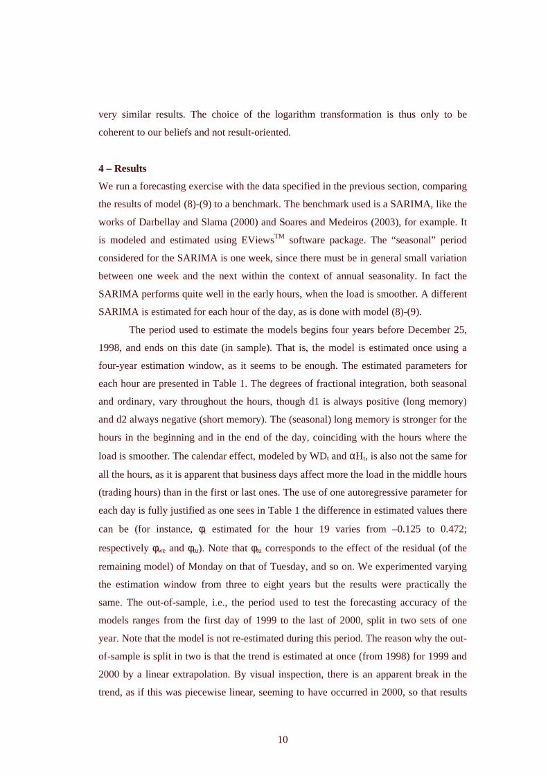
and sometimes two steps ahead, where it is beaten by hour 21. Figure 2 shows the

periodogram (raw and smoothed by a Parzen lag window with degree of smoothness

0.9, respectively represented by dots and a solid line) for the same series in log-log

scale. Note the resemblance with the behavior described by (7). The eighth Fourier

frequency, corresponding to an annual period as we use eight years of data, shows a

sharp peak in the raw periodogram, whereas its vicinity shows a smooth decrease (in

log-log scale) going farther to either side. The subfigure corresponding to hour 20 in

Figure 2 is consistent with the ACF shown in Figure 1, since there are peaks at the

eighth and the sixteenth Fourier frequencies, meaning that there may be one

(semiannual) or two (annual and semiannual) Gegenbauer factors.

We chose working with logarithms as the weekly seasonality and the holiday

effect can be modeled additively while they are multiplicative in the original series X t.

These effects are believed to be multiplicative while relating to consuming habits,

varying proportionally when the number of consumers expands. However, we

experimented applying the same modeling as in (8)-(9) to X t, instead of Y t, yielding

10

very similar results. The choice of the logarithm transformation is thus only to be

coherent to our beliefs and not result-oriented.

4 – Results

We run a forecasting exercise with the data specified in the previous section, comparing

the results of model (8)-(9) to a benchmark. The benchmark used is a SARIMA, like the

works of Darbellay and Slama (2000) and Soares and Medeiros (2003), for example. It

is modeled and estimated using EViewsTM software package. The “seasonal” period

considered for the SARIMA is one week, since there must be in general small variation

between one week and the next within the context of annual seasonality. In fact the

SARIMA performs quite well in the early hours, when the load is smoother. A different

SARIMA is estimated for each hour of the day, as is done with model (8)-(9).

The period used to estimate the models begins four years before December 25,

1998, and ends on this date (in sample). That is, the model is estimated once using a

four-year estimation window, as it seems to be enough. The estimated parameters for

each hour are presented in Table 1. The degrees of fractional integration, both seasonal

and ordinary, vary throughout the hours, though d1 is always positive (long memory)

and d2 always negative (short memory). The (seasonal) long memory is stronger for the

hours in the beginning and in the end of the day, coinciding with the hours where the

load is smoother. The calendar effect, modeled by WDt and αHt, is also not the same for

all the hours, as it is apparent that business days affect more the load in the middle hours

(trading hours) than in the first or last ones. The use of one autoregressive parameter for

each day is fully justified as one sees in Table 1 the difference in estimated values there

can be (for instance, φt estimated for the hour 19 varies from –0.125 to 0.472;

respectively φwe and φtu). Note that φtu corresponds to the effect of the residual (of the

remaining model) of Monday on that of Tuesday, and so on. We experimented varying

the estimation window from three to eight years but the results were practically the

same. The out-of-sample, i.e., the period used to test the forecasting accuracy of the

models ranges from the first day of 1999 to the last of 2000, split in two sets of one

year. Note that the model is not re-estimated during this period. The reason why the out-

of-sample is split in two is that the trend is estimated at once (from 1998) for 1999 and

2000 by a linear extrapolation. By visual inspection, there is an apparent break in the

trend, as if this was piecewise linear, seeming to have occurred in 2000, so that results

11

for this year are likely to be worse than those for 1999. Indeed they are, as one can

inspect by comparing Tables 2.1 and 3.1. The reason for this apparent break may relate

to macroeconomic factors, being beyond the scope of this paper. In a practical

application, it would be wise to frequently re-estimate the model, but in this illustration,

not re-estimating the model allows one to observe that the model does not suffer from

misspecification (remember the trend is forecasted as linear, but not modeled so).

The favorite measure of forecasting accuracy in the load forecasting literature

(c.f. Darbellay and Slama, 2000, Park et al., 1991, and Peng et al., 1992) is the Mean

Absolute Percentage Error (MAPE), which is defined below, as it measures the

proportionality between error and load.

�= +

++ −=

n

i iT

iTiT

X

XX

nMAPE

1

ˆ1

, (10)

where Xt is the load at time t, tX̂ its estimate, T is the end of the in-sample and n is the

size of the out-of-sample. Other measures could be used, as some works suggest that

these measures should penalize large errors and others suggest that the measure should

be easy to understand and related to the needs of the decision makers. For an example of

the former, Armstrong and Collopy (1992) suggest the Root Mean Square Error

(RMSE), while for an example of the latter, Bakirtzis et al. (1996) use Mean Absolute

Errors (MAE). However, both measures lack comparability among different data sets,

and, maybe because of that, the MAPE still remains as the standard measure. Some

authors (c.f., Park et al., 1991, and Peng et al., 1992) achieve MAPEs as low as 2%

when predicting the total daily load, but results of different methods cannot be

compared on different data sets as some data are noisier than others. If different data

sets are used, the same method(s) must be used, and the comparison be made among

data sets and not methods. As to the present data, Table 2 shows the MAPE one to

seven days ahead for the year of 1999 both for the model proposed in this paper and the

SARIMA benchmark. The best method for each hour and number of steps ahead is

shown in bold. The proposed model outperforms the benchmark for all hours at one step

ahead. The benchmark is better mainly for the first five hours and more than one step

ahead. The middle hours see a huge difference in the forecast ability, with our model

performing well, attaining MAPEs of around 3% for one step ahead going to 4% for

seven steps ahead. In contrast, the benchmark attains two-digit MAPEs for steps ahead

higher than one. The peak hours (19-21) see the best MAPEs, in part because the load is

12

the highest in the day (but the proportional predictability is more accurate for both

methods). Table 3 presents the same as Table 2, but for the year 2000. The results are

slightly worse, mainly because the linear trend is not re-estimated but seems to suffer a

break in 2000, as explained before. Even so, the results are good and are qualitatively

equal to the year of 1999, the difference being that the SARIMA fares better also in the

sixth hour for steps ahead higher than one. The worst MAPEs from the model (8)-(9),

namely those for the first hours seven steps ahead, rise from below 7% in 1999 to above

8% in 2000. As to one step ahead results, the best MAPE rises from 2,23% in 1999 to

2,63% in 2000 (hour 21) and the worst from 3,76% (hour 1) to 4,43% (hour 2). The

hour 20 is the best predictable hour for seven steps ahead using the MAPE as the

criterion, yielding MAPEs of 3,12% in 1999 and 3,93% in 2000. It is important to note

that when we speak of h steps ahead, we consider the sectional data and hence refer to

days. As the primary data are hourly, one must interpret as 24h steps ahead, so that (1,

2, …, 7) daily steps ahead actually correspond to (7, 14, …, 168) hourly steps ahead. In

practice, it would be interesting to use the model proposed here and the benchmark,

each one for the hours and time horizons in which each one fares better, or even in a

combined way. The combination is out of the scope of this paper.

Figure 3 illustrates with a typical week the one step ahead forecasting

performance of the proposed model and the benchmark. This week goes from May 9,

1999 to May 15, 1999. One can notice that the forecasts from the proposed model fit

more closely to the observed loads than those from the benchmark do, reflecting the

smaller error obtained by (8)-(9) as presented in Table 2. However, both fits are

reasonably good, and the benchmark is not a bad predictor for this horizon (24 hours

ahead). Figure 4 illustrates the seven steps ahead forecasting performance of the

proposed model and the benchmark, using the same week as Figure 3. The fits are

looser than those for one step ahead, as expected, but the proposed model forecasts still

track the realized loads. The benchmark forecasts, on the other hand, miss out the real

loads too often for this horizon (168 hours ahead), corroborating the superiority of the

proposed model.

5 – Final remarks

This paper proposes a stochastic model for the hourly electricity load demand from the

area covered by a specific Brazilian utility. This model applies to sectional data, that is,

the load for each hour of the day is treated separately as a series. This model can be

13

applied to other utilities presenting similar seasonal patterns, such as many in Brazil.

The model explains the seasonality by generalized (seasonal) long memory using

Gegenbauer processes, having in addition a stochastic level (driven by some trend), and

a calendar effects component (consisting of dummy variables for the days of the week

and for holidays). The Gegenbauer processes fit in well the form of the autocorrelations

observed after the estimated level and calendar effects are removed.

A forecasting exercise against a SARIMA model (the benchmark) is highly

favorable to our modeling. This exercise included the entire years of 1999 and 2000,

forecasting one to seven days ahead (24, 48, …, 168 hours ahead), using models

estimated up to the end of 1998. We conclude for the presence of seasonal long memory

in the data in study and suggest that it may be present in the load demand of other

utilities with similar seasonal behavior as well.

Acknowledgements

The authors would like to thank the Brazilian Center for Electricity Research (CEPEL)

for the data; Dominique Guégan for providing some bibliographical work; and to

Marcelo Medeiros and Reinaldo Souza for invaluable comments on a previous version

of this work. The second author would also like to thank FAPERJ for the financial

support.

References

Armstrong, J.S. and Collopy, F. (1992), “Error measures for generalizing about forecast

methods: empirical comparisons” , International Journal of Forecasting 8, 69-

80.

Arteche, J. (2002), “Semiparametric robust tests on seasonal or cyclical long memory

time series” , Journal of Time Series Analysis 23, 251-285.

Baillie, R.T. (1996), “Long memory processes and fractional integration in

econometrics” , Journal of Econometrics 73, 5-59.

Bakirtzis, A.G., Petridis, V., Kiartzis, S.J., Alexiadis, M.C. and Maissis, A.H. (1996),

“A neural network short term load forecasting model for the Greek power

system”, IEEE Transactions on Power Systems 11, 858-863.

Beran, J. (1994). Statistics for Long Memory Processes (Chapman & Hall, London).

Bunn, D.W. and Farmer, E.D., Eds. (1985). Comparative Models for Electrical Load

Forecasting (John Wiley & Sons, Belfast).

14

Chung, C.-F. (1996), “Estimating a generalized long memory process”, Journal of

Econometrics 73, 237-259.

Darbellay, G.A. and Slama, M. (2000), “Forecasting the short-term demand for

electricity. Do neural networks stand a better chance?”, International Journal of

Forecasting 16, 71-83.

Ferrara, L. and Guégan, D. (1999), “Estimation and applications of Gegenbauer

processes”, working paper.

Ferrara, L. and Guégan, D. (2000), “Forecasting financial time series with generalized

long memory processes: theory and applications”, in C. Dunis (ed.), Advances in

Quantitative Asset Management, Kluwer Academic Press, 319-342.

Ferrara, L. and Guégan, D. (2001), “Forecasting with k-factor Gegenbauer processes:

theory and applications”, Journal of Forecasting 20, 581-601.

Fox, R. and Taqqu, M.S. (1986), “Large-sample properties of parameter estimates for

strongly dependent stationary Gaussian time series” , Annals of Statistics 14,

517-532.

Granger, C. W. G. and R. Joyeux (1980), “An introduction to long memory time series

models and fractional differencing”, Journal of Time Series Analysis 1, 15-29.

Gray, H.L., Zhang, N.-F. and Woodward, W.A. (1989), “On generalized fractional

processes”, Journal of Time Series Analysis 10, 233-257.

Hosking, J. (1981), “Fractional differencing” , Biometrika 68, 1, 165-176.

Hippert, H.S., Pedreira, C.E. and Souza R.C. (2001), “Neural networks for short-term

load forecasting: a review and evaluation” , IEEE Transactions on Power

Systems 16, 44-55.

Mandelbrot, B.B. (1977). Fractals: Form, Chance and Dimension (Freeman, San

Francisco).

Park, D.C., El-Sharkawi, M.A., Marks II, R.J., Atlas, L.E. and Damborg, M.J. (1991),

"Electric load forecasting using an artificial neural network", IEEE Transactions

on Power Systems 6 (2), 442-449.

Peng, T.M., Hubele, N.F. and Karady, G.G. (1992), “ Advancement in the application of

neural networks for short-term load forecasting” , IEEE Transactions on Power

Systems 7 (1), 250-256.

Porter-Hudak, S. (1990), “An application of the seasonal fractional differenced model to

the monetary aggregates”, Journal of the American Statistical Association 85,

338-344.

15

Ramanathan, R., Engle, R., Granger, C.W.J., Vahid-Araghi, F. and Brace, C. (1997),

“Short-run forecasts of electricity loads and peaks”, International Journal of

Forecasting 13, 161-174.

Ray, B.K. (1993), “Long-range forecasting of IBM product revenues using a seasonal

fractionally differenced ARMA model” , International Journal of Forecasting 9,

255-269.

Soares, L.J. and Medeiros, M.C. (2003), “Short-term load forecasting: a two-step

modelling”, working paper.

Souza, L.R. and Soares, L.J. (2003), “Forecasting electricity load demand: analysis of

the 2001 rationing period in Brazil” , working paper.

Whittle, P. (1951). Hypothesis testing in time series analysis (Hafner, New York).

16

Table 1: Parameter estimates of model (8)-(9) for each hour.

hour d1 d2 WDsu WDmo WDtu WDwe WDth WDfr WDsa α φsu φmo φtu φwe φth φfr φsa

1 0.361 -0.370 -0.013 -0.047 0.001 0.006 0.010 0.013 0.031 0.006 0.407 0.695 0.495 0.552 0.289 0.574 0.541 2 0.374 -0.395 -0.013 -0.044 -0.001 0.007 0.010 0.013 0.030 0.015 0.434 0.687 0.513 0.560 0.301 0.558 0.550 3 0.385 -0.407 -0.019 -0.041 0.001 0.010 0.011 0.013 0.025 0.016 0.473 0.665 0.485 0.525 0.335 0.607 0.606 4 0.394 -0.411 -0.026 -0.039 0.003 0.012 0.012 0.015 0.022 0.010 0.450 0.646 0.480 0.582 0.316 0.624 0.639 5 0.398 -0.408 -0.036 -0.034 0.006 0.015 0.015 0.018 0.017 -0.004 0.471 0.617 0.485 0.559 0.331 0.679 0.604 6 0.396 -0.410 -0.063 -0.020 0.015 0.024 0.022 0.023 -0.002 -0.042 0.493 0.537 0.439 0.538 0.338 0.713 0.673 7 0.350 -0.340 -0.121 0.006 0.035 0.042 0.038 0.039 -0.039 -0.126 0.537 0.291 0.400 0.406 0.363 0.700 0.751 8 0.315 -0.280 -0.175 0.028 0.048 0.057 0.052 0.055 -0.066 -0.194 0.613 0.295 0.305 0.340 0.244 0.714 0.620 9 0.280 -0.192 -0.220 0.046 0.059 0.068 0.065 0.068 -0.084 -0.252 0.494 0.309 0.286 0.304 0.096 0.789 0.401 10 0.251 -0.112 -0.246 0.057 0.065 0.072 0.070 0.073 -0.091 -0.285 0.367 0.163 0.278 0.345 -0.002 0.739 0.171 11 0.230 -0.072 -0.257 0.064 0.069 0.076 0.073 0.074 -0.099 -0.300 0.298 0.158 0.389 0.378 0.040 0.527 -0.109 12 0.238 -0.126 -0.257 0.066 0.070 0.078 0.074 0.073 -0.105 -0.306 0.398 0.151 0.379 0.383 0.109 0.631 0.088 13 0.239 -0.140 -0.249 0.066 0.069 0.076 0.072 0.073 -0.105 -0.297 0.439 0.183 0.379 0.354 0.125 0.599 0.089 14 0.244 -0.160 -0.255 0.068 0.072 0.079 0.075 0.075 -0.115 -0.303 0.473 0.338 0.468 0.414 0.116 0.543 0.113 15 0.248 -0.177 -0.261 0.072 0.077 0.085 0.078 0.076 -0.126 -0.311 0.481 0.409 0.511 0.289 0.126 0.547 0.147 16 0.253 -0.201 -0.263 0.073 0.078 0.086 0.080 0.074 -0.128 -0.308 0.508 0.462 0.600 0.212 0.156 0.597 0.208 17 0.219 -0.128 -0.253 0.072 0.075 0.086 0.079 0.066 -0.126 -0.297 0.321 0.336 0.648 -0.029 0.127 0.537 0.128 18 0.198 -0.149 -0.192 0.053 0.054 0.066 0.061 0.048 -0.090 -0.257 0.441 0.165 0.567 -0.024 0.114 0.523 0.203 19 0.271 -0.062 -0.131 0.032 0.039 0.044 0.041 0.030 -0.055 -0.207 0.409 0.086 0.472 -0.125 -0.040 0.296 0.112 20 0.292 -0.121 -0.096 0.021 0.026 0.032 0.028 0.018 -0.029 -0.156 0.526 0.238 0.449 0.127 0.068 0.374 0.203 21 0.279 -0.273 -0.081 0.019 0.023 0.029 0.025 0.015 -0.030 -0.114 0.755 0.457 0.695 0.329 0.439 0.508 0.312 22 0.311 -0.355 -0.072 0.017 0.025 0.030 0.025 0.014 -0.039 -0.097 0.909 0.462 0.608 0.360 0.484 0.523 0.422 23 0.330 -0.346 -0.058 0.010 0.020 0.025 0.023 0.017 -0.038 -0.063 0.776 0.481 0.639 0.350 0.468 0.493 0.461 24 0.343 -0.349 -0.050 0.006 0.010 0.018 0.017 0.024 -0.024 -0.040 0.772 0.477 0.618 0.336 0.509 0.523 0.400

17

Table 2: MAPE for the entire year of 1999 (the best model in bold).

model (8)-(9) SARIMA

steps ahead steps ahead

hour 1 2 3 4 5 6 7 1 2 3 4 5 6 7

1 3.76% 5.14% 5.82% 6.08% 6.30% 6.49% 6.71% 3.93% 4.93% 5.63% 5.84% 5.83% 5.63% 4.72% 2 3.68% 5.09% 5.84% 6.12% 6.33% 6.59% 6.81% 3.85% 4.79% 5.37% 5.51% 5.46% 5.40% 4.67% 3 3.54% 4.97% 5.75% 6.00% 6.18% 6.47% 6.70% 3.67% 4.55% 5.21% 5.36% 5.26% 5.14% 4.40% 4 3.35% 4.67% 5.54% 5.73% 5.92% 6.18% 6.40% 3.46% 4.39% 5.07% 5.24% 5.20% 5.02% 4.17% 5 3.21% 4.39% 5.20% 5.39% 5.56% 5.83% 6.04% 3.37% 4.16% 4.95% 5.18% 5.16% 4.90% 4.01% 6 2.91% 4.09% 4.70% 4.93% 5.07% 5.35% 5.54% 3.26% 4.31% 5.29% 5.90% 5.95% 5.43% 4.30% 7 2.85% 3.69% 4.16% 4.30% 4.43% 4.63% 4.72% 3.62% 6.21% 8.24% 9.08% 9.16% 8.42% 6.27% 8 2.74% 3.37% 3.75% 3.88% 4.04% 4.22% 4.31% 4.09% 8.43% 11.04% 11.80% 11.99% 11.38% 8.38% 9 2.75% 3.45% 3.76% 3.86% 3.98% 4.12% 4.21% 4.63% 10.33% 13.18% 13.76% 13.98% 13.62% 10.05% 10 2.82% 3.46% 3.78% 3.86% 3.93% 4.00% 4.07% 4.91% 11.38% 14.42% 14.89% 15.07% 14.84% 11.05% 11 2.92% 3.59% 3.86% 3.97% 4.01% 4.04% 4.05% 4.95% 11.81% 15.19% 15.48% 15.67% 15.57% 11.40% 12 2.89% 3.61% 3.88% 3.96% 3.97% 3.98% 4.00% 5.02% 12.06% 15.61% 15.81% 15.93% 15.96% 11.58% 13 2.99% 3.79% 4.07% 4.17% 4.19% 4.19% 4.24% 5.04% 11.69% 15.32% 15.64% 15.72% 15.50% 11.19% 14 3.15% 4.06% 4.40% 4.51% 4.49% 4.49% 4.52% 5.10% 12.01% 15.91% 16.14% 16.20% 16.04% 11.45% 15 3.22% 4.16% 4.52% 4.63% 4.67% 4.67% 4.73% 5.16% 12.45% 16.78% 17.08% 17.16% 16.89% 11.79% 16 3.21% 4.11% 4.48% 4.60% 4.70% 4.74% 4.77% 5.11% 12.40% 16.92% 17.33% 17.34% 16.93% 11.70% 17 3.26% 3.84% 4.17% 4.27% 4.35% 4.40% 4.43% 4.82% 11.57% 16.16% 16.57% 16.64% 16.11% 10.97% 18 2.95% 3.49% 3.71% 3.79% 3.81% 3.85% 3.90% 4.27% 8.97% 11.95% 12.46% 12.56% 12.19% 8.65% 19 2.82% 3.38% 3.57% 3.73% 3.87% 3.94% 3.99% 3.54% 6.04% 7.55% 8.02% 8.01% 7.89% 6.12% 20 2.35% 2.87% 2.93% 3.04% 3.05% 3.07% 3.12% 3.07% 4.90% 5.63% 5.98% 5.94% 5.77% 4.88% 21 2.23% 2.83% 3.10% 3.21% 3.27% 3.35% 3.47% 2.85% 4.47% 5.44% 5.84% 5.82% 5.44% 4.42% 22 2.56% 3.39% 3.75% 3.88% 3.93% 4.02% 4.13% 3.08% 4.85% 6.21% 6.73% 6.70% 6.09% 4.76% 23 3.04% 3.99% 4.45% 4.66% 4.72% 4.87% 5.01% 3.35% 4.83% 6.18% 6.67% 6.55% 6.07% 4.63% 24 3.54% 4.75% 5.33% 5.60% 5.72% 5.92% 6.10% 3.76% 4.97% 6.00% 6.38% 6.34% 5.93% 4.76%

18

Table 3: MAPE for the entire year of 2000 (the best model in bold).

model (8)-(9) SARIMA

steps ahead steps ahead

hour 1 2 3 4 5 6 7 1 2 3 4 5 6 7

1 4.37% 6.42% 7.38% 7.92% 8.18% 8.20% 8.16% 4.53% 5.77% 6.55% 6.71% 6.73% 6.65% 5.70% 2 4.43% 6.54% 7.62% 8.15% 8.43% 8.45% 8.42% 4.53% 5.73% 6.42% 6.55% 6.54% 6.50% 5.65% 3 4.37% 6.45% 7.61% 8.15% 8.46% 8.44% 8.45% 4.44% 5.58% 6.27% 6.36% 6.35% 6.33% 5.48% 4 4.23% 6.24% 7.40% 7.93% 8.26% 8.28% 8.26% 4.35% 5.30% 6.05% 6.15% 6.15% 6.06% 5.24% 5 4.03% 5.99% 7.12% 7.69% 8.01% 8.06% 8.09% 4.24% 5.07% 5.82% 5.92% 5.97% 5.87% 5.11% 6 3.81% 5.60% 6.58% 7.05% 7.32% 7.40% 7.46% 4.14% 5.10% 6.21% 6.48% 6.46% 6.16% 5.14% 7 3.60% 5.08% 5.88% 6.21% 6.43% 6.53% 6.59% 4.47% 6.93% 8.68% 9.12% 9.16% 8.72% 6.57% 8 3.22% 4.61% 5.26% 5.54% 5.73% 5.81% 5.88% 4.70% 9.08% 11.41% 12.08% 12.13% 11.58% 8.61% 9 3.03% 4.28% 4.75% 5.03% 5.22% 5.30% 5.35% 4.92% 10.69% 13.48% 14.28% 14.33% 13.86% 10.25% 10 2.97% 4.06% 4.49% 4.67% 4.80% 4.86% 4.92% 5.24% 12.01% 15.02% 15.80% 15.85% 15.52% 11.48% 11 3.00% 3.97% 4.39% 4.56% 4.69% 4.76% 4.81% 5.39% 12.69% 16.11% 16.81% 16.79% 16.53% 11.99% 12 3.05% 3.99% 4.41% 4.56% 4.68% 4.73% 4.75% 5.60% 12.78% 16.47% 17.14% 17.12% 16.84% 12.10% 13 3.00% 4.00% 4.44% 4.59% 4.71% 4.76% 4.78% 5.40% 12.56% 16.27% 16.94% 16.93% 16.49% 11.71% 14 3.17% 4.29% 4.72% 4.93% 5.05% 5.10% 5.10% 5.55% 12.85% 16.80% 17.65% 17.60% 17.09% 12.11% 15 3.38% 4.51% 4.98% 5.19% 5.31% 5.35% 5.36% 5.74% 13.29% 17.70% 18.40% 18.45% 17.89% 12.41% 16 3.43% 4.55% 4.98% 5.23% 5.33% 5.41% 5.43% 5.77% 13.17% 17.77% 18.47% 18.57% 17.90% 12.29% 17 3.60% 4.43% 4.77% 4.89% 4.98% 5.04% 5.02% 5.39% 12.19% 16.65% 17.26% 17.39% 16.63% 11.25% 18 3.44% 4.19% 4.43% 4.52% 4.58% 4.58% 4.59% 4.79% 9.24% 12.18% 12.66% 12.68% 12.09% 8.67% 19 3.21% 3.77% 4.07% 4.30% 4.44% 4.50% 4.53% 4.03% 6.43% 7.81% 8.13% 8.14% 7.80% 6.18% 20 2.71% 3.30% 3.60% 3.74% 3.87% 3.93% 3.93% 3.47% 5.15% 5.74% 5.95% 6.05% 5.80% 4.99% 21 2.63% 3.45% 3.85% 4.11% 4.16% 4.23% 4.22% 3.17% 4.89% 5.67% 5.84% 5.95% 5.69% 4.56% 22 2.98% 4.12% 4.62% 4.94% 5.11% 5.17% 5.16% 3.36% 5.30% 6.61% 6.92% 6.90% 6.56% 4.92% 23 3.58% 5.15% 5.82% 6.22% 6.41% 6.43% 6.41% 3.99% 5.64% 6.95% 7.28% 7.24% 6.79% 5.30% 24 4.14% 5.96% 6.81% 7.34% 7.56% 7.60% 7.56% 4.50% 5.79% 6.78% 7.09% 6.98% 6.70% 5.59%

19

Figure 1: Autocorrelation function of the series from January 1, 1990 to December 31, 1998, for hours 1, 8, 14 and 20, after removal of the trend and the calendar effects (weekdays and holydays), up to lag 1000. Note the resemblance to a damped sinusoid.

20

Figure 2: Raw and smoothed periodogram of the series from January 1, 1990 to December 31, 1998, for hours 1, 8, 14 and 20, after removal of the trend and the calendar effects.

21

Figure 3: Real versus predicted load (MWh), for both the model proposed here and the SARIMA benchmark, one step ahead, from May 9, 1999 to May 15, 1999 (one week, from Sunday to Saturday).

22

Figure 4: Real versus predicted load (MWh), for both the model proposed here and the SARIMA benchmark, seven steps ahead, from May 9, 1999 to May 15, 1999 (one week, from Sunday to Saturday).

���������������������� ��������� ������ ������������������� ���������������� �!"�����#���$�%&��� ������')(*� ���,+-��.#����������0/#��132�465

��798,73: ;373<>=@?���134A4613?B4679C�D�5E35GF�?H;9=I5�4J� KLKL: 134 CMN73OQP13:�2�1R'JS�4613PT��13KUKLV7R/W%&7346X35Y2�1[Z]\�\]Z_^`Z]ab�c3d KL�

���]Z]� ��. ����&����� ����� ��(U�e���&����%&���>��� ��� F��&��� ��(����!�>'J�-��������� ���f/g�4673<hG.�����7 d 1iD�4 C0��73P: 5kj]�%&5<l=I13?H4A5m/n'JS�46?B:L2�1MZ]\�\]Z)/o�]� b�c3d KL�

���]p]� �q%&����'J��� �%&�q%&� ���>��rJ�����q���s����'J�!�%&� ��t)�u��'*������!� %&� '*v ��'J�� (U�����'W��w �^x��(@'J�!����>'J(y/o%&7346;313: 5z�1346<73<2�13K{C|D�P�73<m��5465m/n'JS�46?B:L2�1MZ�\]\]Z)/op�p b�c3d KU�

���]�]� '}��� v�����T����Fy�����~u����� ���(������ �fv���'y��� (i���� ���e%&��(I��� ��(U�R�|'y��'�N���������R/q�4673<;3?HKU;35.��������13464613?B4679C���19=@134N(U73<>��5P>�iC�%&734A;313: 5z��134A?9/n'JS�46?B:L2�1MZ]\�\]Z)/op]a b�c3d KL�

���]�]� ��. ��%&���N���!� (����!j]������ ������. ����v��� ������N���� � ���!� � ��'y��������� ��� �������������� ���!����������R')���Y(U�>'J�����!�f� ����������&� �Q���� �!��%&� �R')����� Fy� ��~R/GD�5E35JFy?B;9=@54���KUKL: 134 C��7346KL�?B2Fy73�?B2�/o%&73?B5z2�1�Z]\]\�ZJ/&p�� b�c3d KL�

���]�]� ��������(@'y��� F���'y����'J��j]_� �e� �v|�������� (U(I'J��� �3'y��� ���&'J�!�o���L����%&��%"�����������!��~i'J���>'Jz/'J: 5?BKL?B5m'J4673P>��5>C�%&7346;3?B7M(�135<m/o%&73?B5z2�1MZ�\]\�ZJ/o��� b�c3d KL�

���]�]� Fy� ����'J� ����'J��� ��'J(I��������� ������� ���'J���q���>Fy�(�����%&�����/q�73OiP�13:�2�1�'JS�4A13PR��13KLKL579C���79��7313:��5S�/o%&73?B5z2�1MZ�\]\�ZJ/o��p b�c3d KL�

���]a]� ����F�������%&����W'J������� ��*����N������� ������� ����������� � ��������/}'J�#����Fy��������'y����� �`� �����N�� v (���%&�>'J������_���� %���. ��������� ���l')������� ���&/[��134AO c <���73: ��79=6C ��13<79=@5�� �]�: V4613K�D�46�/nD�P<�5z2�1�Z]\]\�ZJ/&p]\ b�c3d KL�

���]�]� ' %&�����(k� �T��'J��� ��')(i'J������%&��(I'y����� ��'J�!�*�������^x���j]���!��/*��73P: 5Yv�734613: : ? C�N73OQP13:�2�1'JS�4613Pz��13KLKUV�7!/nD�P<�5z2�1MZ�\]\�ZJ/o��\ b�c3d KL�

���]\]� ��. ��%&���N���!� (����!j]������ ������. ����v��� ������N���� � ���!� � ��'y��������� ��� �������������� ���!����������R')���Y(U�>'J�����!�f� ����������&� �Q���� �!��%&� �R')����� Fy� ��~R/GD�5E35JFy?B;9=@54���KUKL: 134 C��7346KL�?B2Fy73�?B2�/nD�P<�5z2�1�Z]\]\�ZJ/&Z]� b�c3d KL�

������� (U��!�����`(U� 'Jv���(�� ��~¡���¡��.������ ��N��%&������������ �`%Q')��j]�>��/¢�: ?BKL73S�19=6=@7£� 5KLKL79Cu��?BP: ?B73<7��73: POQS�5m/n' d 5K{=@5z2�1MZ]\�\]Z)/oZ]\ b�c3d KU�

���]Z]� ���������� ��������(��i'J�!�Y� ���� ��%Q'y����� �-������F����� ���!�,%&���!� ��� �����!�GF�������_%Q'J�!������(@'y����� �^y�: ?BKU73S�19=6=I7M��5KLKU79C�� ?HP: ?B73<7M��73: POiS�5m/n' d 5K{=I5z2�1MZ�\]\�ZJ/op�� b�c3d KL�

���]p]� ��� �������'J��� � ��� %&�>�������¤')��������¥� �¦���������� (U� � � �L����%&��'y����� ��+�� ��. . ��� . ���%&��%&�����z/o� PK{=@798,5z%&��2�1!'y=@�79§�2�19C���13<79=@5z���¨��: V4613K�D�46��/&�19=@13OiS�465z2�1MZ�\]\]Z)/oZ�� b�c3d KU�

���]�]� %&���N����'J�!��� ' ����������©�tJ� ���������ª ��� ��' � ���������')����� ��')( �% ���� �!��%&� ' �������« ����'J��������¬�Y�����L')����')%&��������¬v���'JN��(������� T^)D�5E35GF�?B;9=@54J��KLKU: 134 C���79=@?B73<�7o��73: 2�73K2�1�(U?BOQ7!'J;3�­M��?B: : 734�/&�19=@13OiS�465z2�1MZ�\]\]Z)/op�� b�c3d KU�

���]�]� ������� ���������������� ��F�����%&�����N����(�(U��Fy���N� 'J����� ����� ��'J(&(U�N�� ��g���� %®'¯������������~������|~_^���13<79=@5�������: 5�4A13K�D�4HC!%&7346?B7n��73P: 7n�5<l=I5�P4679C���5 d ­346?B5R� P1346467nN73<l=I5�K)/qN19=@13OQS�465R2�1Z]\�\]Z)/op]\ b�c3d KL�

���]�]� '0����������'J����� F��_%&�>��.�� ���� �u��� %&���������!�[��.��G���'y����� ��'J��~q�� (U�,��� �������z��.��G���(�����«��,'y��� ���k^�+}?B: ��46132�5z(U��%&73: 2�5<732�5lC�.�POQS�134 =@5z%&54613?B467!/o�19=@13OiS�4A5z2�1MZ�\]\�ZJ/��¨� b�c3d KL�

���]�]� ����'J��� (U� v�����'J(U� �3'y����� ��'J������. � �>Fy� (�������� �"��� Nj]� (U(u�>'J���!���!� �� � ������������ 'J(�����v���'y����(�^�� PK{=@798�5 � 5< � 7 d 79C �!73­346;3?B5�%&13<1 � 13K��?B: �5>C ��46?BK{=@?B<7m��1346467m/oN19=@13OQS�465z2�1MZ]\�\]Z)/op��b�c3d KL�

���]a]� ����N�%&�����!. �¯�������� %Q'J�������£���uFy� (I'y��� (U� �|'J������'¢v�� (U'¢���uF�'J(�������0����tJ��L'J��(��n^yv�1346<73462�5z2�1M c %&5>=@79C�%&7346;313: 5z�1346<73<2�13K�/o� Pl=IP�S�465z2�1MZ]\�\]Z)/op]� b�c3d KU�

���]�]� ������� ���¬����!�����!�_���_')� �%&������� ���f%Q')��j]�>�����.��i%&���!�>��')��~[�����%&����%���.��� ��~R'J�!���. �gv���'y����(�� ')�#��')��>�Y�������x^������]aq^&��7346: 5�K�.�73Oi?B: =@5<TFy��'J467��>��5>C���13<79=@5¬� ���: 54613K&D�46��/��P>=@PS�465z2�1MZ]\�\]Z)/o�]� b�c3d KL�

���]\]� ��������%Q'������lF�������!��� rJ��� 'J�,�%"v������'g��� � ����������� F��� �L'J��'f'y����'J� �k�R����')v�')(U.�'J�����'J����� ��� %&�o^��73Oi73<l=I��7���7373O¯��734 =AC!%&7346;313: 5���V4 =@13Ki��1346? C!�: 798,?B5�%&13<1 � 13K�/e�!5>8,13OQS�465�2�1Z]\�\]Z)/oZ]a b�c3d KL�

������� ������������+}� ��j�'J�!� ��. � � ���� ��%Q'J(�N������ �¡��� v���'y����(g/ %&7346;313: 5 ��V4 =@13K£�!1346?z/��5>8,13OiS�4A5z2�1MZ�\]\�ZJ/������ b�c3d KL�

���]Z]� ����(�ª ������'¦����������'J �����!��(���tJ������'Jv|'J(U. ����'$�|'J��������'J���� % �������������!��� '#^%&7346;313: 5k��V�4H=@13K���1346? C�'J: 1��73<2�4A1_��?B<>=@5k2�1_��734 8�73: �5lC�.�13KUKL?B7_� P?B: �1346OQ5k��5�K@=@?B: : 7�/¬�!5l8�13OQS�4652�1�Z]\]\�ZJ/&�]� b�c3d KL�

���]p]� ��(��l��� F����|'J�����£%&������|'J ���£« ��'J(����|'J���£�|' �� ����'J©�t)�¡v ��'J�� (U�����' �¨�]�]�¨^IZ�\]\���^%&7346;313: 5z��V4 =I13Ks�!1346? C|'J: 1��73<2�461M��?B<>=@5z2�1M��734 8,73: ��5m/&��5>8,13OiS�465z2�1MZ�\]\]Z)/op�p�� b�c3d KL�

���]�]� v���'y����(�� ')� %Q'J���������� ��� %&����¥+}� ��. ' . ��%Q')� �>'J�����%&�>��������� (�� ��'J� ������N�������,F������~i'J�!�&�� ��� 'J(y��'J�����>���/o%&734A;313: 5z��V4 =@13K���134A?9/o��5>8,13OiS�4A5z2�1MZ�\]\�ZJ/o��� b�c3d KL�

���]�]� ����v����>�3'y� 'y��� F�����W'�����W�!�"v���'JN��(T^Y%&7346;313: 5W��V�4H=@13Kg��1346? Ci+}7 d <134G(U��N5�734A13KT/��1 � 13OQS�465z2�1MZ]\�\]Z)/oZ]� b�c3d KL�

���]�]� ���!�(@'J©�tJ� � �(U� ��� v � (U� �|'J���#'J(@')��� 'J(}^}%&7346;313: 5 ��V4 =@13K¯��1346? C�%&73P4��B;3?B5 ��?B<�13?B465£/��1 � 13OQS�465z2�1MZ]\�\]Z)/���� b�c3d KL�

���]�]� ���������� v �,��� Fy�T�����������g� �fv���'y����(�� ')�����������������'J(&��������%&f^i%&7346;313: 5T��V4 =@13K&�!1346? CD�5KL­�% c 46;3?B5z��73OQ734 d 5m/o��1 � 13OiS�465z2�1MZ�\]\]Z)/op�a b�c3d KU�

���]a]� �k���%&���q�|'JY����� 'J�!©�'JR^m%&7346;313: 5R��V4 =@13K �!1346? C���73<�?B13: 7Q��5K{=@7s/u� 1 � 13OQS�465R2�1QZ]\]\�Z�/g���b�c3d KL�

���]�]� �%&��(U��~�%&����[')���¬����� ��������� F�� ��~-����v���'y��� (R���-��.��k�!���!�>��� �&^�D�5�KU­_% c 46;3?B5k��73OQ734 d 5>C%&7346;313: 5z��V4 =I13Ks�!1346? C�%&73P4��B;3?B5z��54 =@1 � ��13?HK�/o��1 � 13OiS�465z2�1MZ�\]\]Z)/op�Z b�c3d KU�

���]\]� ��. �W'J(�� 'JN���!� ���������� ��. ����lD���`j]����!�( 'J���¯���%&������'J(U(I~ 'J��� �����'y����¡(����!�%&�%&����~_����� ����N��z^�(U135<73462�5z���]N5�P � 7!/nD�73<13?B465z2�1MZ]\�\]p)/op]Z b�c3d KL�

������� �������q���R��� ��(U�u���� ����%&� ���u���uv���')���(z�%#��%`%&� ���(U�u��� %`����������©�tJ�_'*�������� ���^sv c 4AS�73467�Fy73KU;35<�;313: 5�K�v�5798,?BK{=@7 2�7 ��P<��79C���132�4A5k��798,73: ;373<>=@?���134A4613?B467 /YD�73<13?B465_2�1 Z�\]\�pQ/Z�� b�c3d KL�

���]Z]� ��. �"��� ��� � �"�������'y����� ���¬(����!���>F�� ��~ 'J��� ��. ������Fy�����~ ������'y����� ���^���132�465��798,73: ;373<>=@?3�13464A13?H4A79C��73OiP�13:U2�1!'JS�4A13Pz��13KLKL57�/QD�73<13?B465z2�1�Z]\]\�pJ/&p�� b�c3d KL�

���]p]� ' � ������')(U� �3'y��� ���¦� ��D��������A %&�>��.�� ��� �£���,��^x����>'J�|~]^I��'����£����%&�L'J������ �!"��������������}������N��� .,�}%&� ���(U-^G��73P: 5�v 734A13: : ? CnN73OQP13:�2�1&')S�4613Pe��13KLKU57&/0�198,134613?B465e2�1Z]\�\]p)/o� b�c3d KL�

���]�]� 'J}(U�� �|'`�>'J( ��!��� ')����%Q'�'Jv�� ���|'J� ��%����� � � %&����'�^z'J: 5 �BKU?H5���13KLKU5�7e2�1o'J4A7��l��5o/�198,134613?B465z2�1MZ]\�\]p)/oZ]� b�c3d KL�

���]�]� ��. �f(����!��^I�������������!��%&� ��� %&�L'J����� � 'J� � f^i��132�465f��798,73: ;373<l=I?y���!�13464613?B4679CM�73OQP13:�2�1'JS�4613Pz��13KLKU5�7!/o�198,134613?B465z2�1MZ]\�\]p)/op]\ b�c3d KL�

���]�]� ' %&� ���>��'J��~`%&���.,')��� �% �� �`�.�'J��� ���¢��')��� ��'J(U�_� � 'J%&� ��� ')�����|~�v�F����¡%&��>�j]� ~�����'Jj��¨')���Q+}����� .,��/o��?B;373462�5z2�1M������798,73: ;373<>=@?9/&��198�134613?B465z2�1�Z]\]\�pJ/e��� b�c3d KL�

���]�]� ����'J�|' �����!��� ����� ��-��%&��(I~f��.�'y� ��������������� ���0����!����� ���0%&���¬v���')�~�%&�L������� ��'J(�(@~��� v v|^x� � ��� (I'J�^���73P: 5zv�734613: : ? C�N73OQP13:L2�1�'JS�4613Pz��13KUKL57�/o%&7346X35z2�1MZ�\]\]p)/o� b�c3d KL�

���]a]� ���%&��� ��'J($'J� � ����,'y����� � 'J�!� v|'J�!��+����|��. N�(U�������� � ��� ������%Q'���� ��� (����!�%&�%&����~ ^�(U135<73462�5z���]N5�P � 7!^y%&7346X35z2�1MZ�\]\]p)/��¨� b�c3d KU�

���]�]� '��!�����f� ����� (U�G'J���*�������j�%Q'J�*^i��73P: 5fv�734613: : ? CM�73OQP13:�2�1�'JS�4613PY��13KLKL57R/�')S�46?B:�2�1Z]\�\]p)/oa b�c3d KL�

��a]\]� 'W. ����w�����N�n�|'Jo� ���������'���� FN'Jo��'W������,������'e'������%&�u���sD�������o�!�uv���'J�� (U����%Q''J��(�����'J©�tJ� ���g%&� � �(���0���uF�'J(�����������������f^Q'J: 1��73<�2�461¬%&73?B7 ��5464A13?H7-(U?BOQ79C�D�5E35Fy?B;9=@54N��KLKU: 134�/&%&73?H5z2�1MZ�\]\]p)/op�\ b�c3d KU�

��a���� ������.��k+}�(��l')���q����������qv���N���!��*��~���(���� ����. �uZ]\���.}�����������~�^�D�5E35_F�?H;9=I5�4��KUKL: 134 C�'y��5<KL5�')46?B<�5Kz2�1i%&13: : 5Q�4673<;35>C���KUOQ73<?¨��13? ��13?B467�2�1���734 8�73: �5i� P?H: : ­3<J/Y%&73?B5 2�1�Z]\�\]p/oZ]� b�c3d KU�

��a]Z]� ���>��� ���!��-')��� ��%Q'J� ��-������'y������ 'J���� ������rJ��� 'J-^G%&7346;35&'J<>=@5<?H5ev�5<�5Oi5lCi� 8,73<7��73: : �B' d <�5:@/nD�P<�5z2�1MZ�\]\�pJ/oZ�� b�c3d KL�

��a]p]� �>Fy� (U��©�tJ�e�|'}����� � �,��� Fy� �|'J���z������'J(���� Y�>'y��������[��'����� ��� %&� 'Wv ��'J�� (U�����'J����%Q''J��rJ(U� ��G��� %&�L'J��'y��� F�'¬^yF�?H;9=I5�4�� 5OQ13K@C!�73OQP13:|2�1�'JS�4613P���13KLKU5�79C �1346<73<2�5z'���Fy13: 5�KU5M/D�P<�5z2�1MZ�\]\�pJ/o��� b�c3d KL�

��a]�]� %&��� ��'J©�t)�,��N�(U�©�tJ�[�������������©�') ���� ��� ��')��G� �z�����!�|'¬�!�ov ��'J�� (�^��<13K{=@54�2�7M��5KU72�5KzN73<l=I5�KmD�P<�?B54 C���73­34A;3?H5 %&13<1 � 13KM�?B: �5>C���132�465 ��798,73: ;373<>=@?��13464613?B467�/�D�P<�5i2�1�Z]\]\�ps/YZ]pb�c3d KL�

��a]�]� ��. �}����Nj0������%&� ��% � �¢v���'y����(�� ')�®� ��Fy����!%&���� ���v����e�¨�]����^IZ�\]\�Zg^G'J<2�4A­W�5734613K(U5P4613?B465>C��1346<73<2�5z2�1M. 5: 73<2�7Mv�7346S�5KL7�^�D�P�<�5z2�1MZ]\�\]p)/���� b�c3d KL�

��a]�]� ��������')������!�-�(U�������� ��� ��~q���%Q'J���e��N���!��� ������')(U� �����q(����!�e%&��%&� ��~ ^)(�73;3?H4�D�54 d 1�5734613K@C�(U135<73462�5z��5;3�7M�5P � 7�/nD�P<��5z2�1MZ]\�\]p)/oZ]Z b�c3d KU�

��a]�]� ��N���!� �����������(@'J��(@~ N�L'J���� ���>������������ ����� %Q'y����%&��(@��� ^x�>'J������� %&� ���(UN�'J����(�����'y����� �T���fv���'y����(�� ')� �«���� ��~[��'���'q^�rJ: 8�73465�F�13? d 79C�(U135<73462�5Q��5;3�7 �5P � 7J/GD�P<�52�1�Z]\]\�pJ/&Z]� b�c3d KL�