BioMed CentralBMC Bioinformatics

ss

Open AcceMethodology articleOptimization of neural network architecture using genetic programming improves detection and modeling of gene-gene interactions in studies of human diseasesMarylyn D Ritchie, Bill C White, Joel S Parker, Lance W Hahn and Jason H Moore*

Address: Program in Human Genetics and Department of Molecular Physiology and Biophysics, Vanderbilt University Medical School, Nashville, TN, 37232-0700, USA

Email: Marylyn D Ritchie - ritchie@phg.mc.vanderbilt.edu; Bill C White - bwhite@phg.mc.vanderbilt.edu; Joel S Parker - parkerjs@email.unc.edu; Lance W Hahn - hahn@phg.mc.vanderbilt.edu; Jason H Moore* - moore@phg.mc.vanderbilt.edu

* Corresponding author

AbstractBackground: Appropriate definition of neural network architecture prior to data analysis iscrucial for successful data mining. This can be challenging when the underlying model of the data isunknown. The goal of this study was to determine whether optimizing neural network architectureusing genetic programming as a machine learning strategy would improve the ability of neuralnetworks to model and detect nonlinear interactions among genes in studies of common humandiseases.

Results: Using simulated data, we show that a genetic programming optimized neural networkapproach is able to model gene-gene interactions as well as a traditional back propagation neuralnetwork. Furthermore, the genetic programming optimized neural network is better than thetraditional back propagation neural network approach in terms of predictive ability and power todetect gene-gene interactions when non-functional polymorphisms are present.

Conclusion: This study suggests that a machine learning strategy for optimizing neural networkarchitecture may be preferable to traditional trial-and-error approaches for the identification andcharacterization of gene-gene interactions in common, complex human diseases.

BackgroundThe detection and characterization of genes associatedwith common, complex diseases is a difficult challenge inhuman genetics. Unlike rare genetic disorders which areeasily characterized by a single gene, common diseasessuch as essential hypertension are influenced by manygenes all of which may be associated with disease risk pri-marily through nonlinear interactions [1,2]. Gene-geneinteractions are difficult to detect using traditional para-metric statistical methods [2] because of the curse of

dimensionality [3]. That is, when interactions amonggenes are considered, the data becomes too sparse to esti-mate the genetic effects. To deal with this issue, one cancollect a very large sample size. However, this can be pro-hibitively expensive. The alternative is to develop new sta-tistical methods that have improved power to identifygene-gene interactions in relatively small sample sizes.

Neural networks (NN) have been used for supervised pat-tern recognition in a variety of fields including genetic

Published: 07 July 2003

BMC Bioinformatics 2003, 4:28

Received: 12 March 2003Accepted: 07 July 2003

This article is available from: http://www.biomedcentral.com/1471-2105/4/28

© 2003 Ritchie et al; licensee BioMed Central Ltd. This is an Open Access article: verbatim copying and redistribution of this article are permitted in all media for any purpose, provided this notice is preserved along with the article's original URL.

Page 1 of 14(page number not for citation purposes)

BMC Bioinformatics 2003, 4 http://www.biomedcentral.com/1471-2105/4/28

epidemiology [4–12]. The success of the NN approach ingenetics, however, varies a great deal from one study tothe next. It is hypothesized that for complex human dis-eases, we are dealing with a rugged fitness landscape[9,13], that is, a fitness landscape with many local minimawhich make it more difficult to find the global minimum.Therefore, the inconsistent results in genetic epidemiol-ogy studies may be attributed to the fact that there aremany local minima in the fitness landscape. Training aNN involves minimizing an error function. When thereare many local minima, a NN using a hill-climbing algo-rithm for optimization may stall on a different minimumon each run of the network [9].

To avoid stalling on local minima, machine learningmethods such as genetic programming [14] and geneticalgorithms [15] have been explored. Genetic program-ming (GP) is a machine learning methodology that gener-ates computer programs to solve problems using a processthat is inspired by biological evolution by natural selec-tion [16–20]. Genetic programming begins with an initialpopulation of randomly generated computer programs,all of which are possible solutions to a given problem.This step is essentially a random search or sampling of thespace of all possible solutions. An example of one type ofcomputer program, called a binary expression tree, isshown in Figure 1.

Binary expression tree example of a GP solutionFigure 1Binary expression tree example of a GP solution. This figure is an example of a possible computer program generated by GP. While the program can take virtually any form, we are using a binary expression tree representation, thus we have shown this type as an example.

Page 2 of 14(page number not for citation purposes)

BMC Bioinformatics 2003, 4 http://www.biomedcentral.com/1471-2105/4/28

Next, each of these computer programs are executed andassigned a fitness value that is proportional to its perform-ance on the particular problem being solved. Then, thebest computer programs, or solutions, are selected toundergo genetic operations based on Darwin's principleof survival of the fittest. Reproduction takes place with asubset of the best solutions, such that these solutions aredirectly copied into the next generation. Crossover, orrecombination, takes place between another subset ofsolutions. This operation is used to create new computerprograms by combining components of two parent pro-grams. An example of a crossover event between two solu-tions is shown in Figure 2.

Thus, the new population is comprised of a portion ofsolutions that were copied (reproduced) from the previ-ous generation, and a portion of solutions that are theresult of recombination (crossover) between solutions ofthe parent population. This new population replaces theold population and the process begins again by executingeach program and assigning a fitness measure to each ofthem. This is repeated for a set number of generations oruntil some termination criterion is met. The goal is to findthe best solution, which is likely to be the solution withthe optimal fitness measure.

Koza [17,18] and Koza et al. [19] give a detailed descrip-tion of GP. A description of GP for bioinformatics appli-cations is given by Moore and Parker [13]. Evolutionary

GP crossoverFigure 2GP crossover. This figure shows a crossover event in GP between two binary expression trees. Here, the left sub-tree of parent 1 is swapped with the left sub-tree of parent 2 to create 2 new trees.

Page 3 of 14(page number not for citation purposes)

BMC Bioinformatics 2003, 4 http://www.biomedcentral.com/1471-2105/4/28

computation strategies such as GP have been shown to beeffective for both variable and feature selection withmethods such as symbolic discriminant analysis formicroarray studies [13,16,21]. Koza and Rice [14] havesuggested GP for optimizing the architecture of NN.

The goal of this study was to implement a GP for optimiz-ing NN architecture and compare its ability to model anddetect gene-gene interactions with a traditional back prop-agation NN. To achieve this goal we simulated data froma set of different models exhibiting epistasis, or gene-geneinteractions. We applied the back propagation NN(BPNN) and the GP optimized NN (GPNN) to these datato compare the performance of the two methods. We con-sidered the GPNN to have improved performance if 1) ithad improved prediction error, and/or 2) it had improvedpower compared to the BPNN. We implemented cross val-idation with both the BPNN and GPNN to estimate theclassification and prediction errors of the two NNapproaches. Based on our results, we find that GPNN hasimproved prediction error and improved power com-pared to the BPNN. Thus, we consider the optimization ofNN architecture by GP to be a significant improvement toa BPNN for the gene-gene interaction models and simu-lated data studied here. In the remainder of this section,we will provide background information on the BPNN,the GPNN strategy, and the cross validation approachused for this study.

Back propagation NN (BPNN)The back propagation NN (BPNN) is one of the mostcommonly used NN [22] and is the NN chosen for manygenetic epidemiology studies [4–12]. In this study, weused a traditional fully-connected, feed-forward networkcomprised of one input layer, zero, one, or two hiddenlayers, and one output layer, trained by back propagation.The software used, the NICO toolkit, was developed at theRoyal Institute of Technology, http://www.speech.kth.se/NICO/index.html.

Defining the network architecture is a very importantdecision that can dramatically alter the results of the anal-ysis [23]. There are a variety of strategies utilized for selec-tion of the network architecture. The features of networkarchitecture most commonly optimized are the number ofhidden layers and the number of nodes in the hiddenlayer. Many of these approaches use a prediction error fit-ness measure, such that they select an architecture basedon its generalization to new observations [23], while oth-ers use classification error, or training error [24]. We choseto use classification error rather than prediction error as abasis for evaluating and making changes to the BPNNarchitecture because we use prediction error to measurethe overall network fitness. We began with a very smallnetwork and varied several parameters including the

number of hidden layers, number of nodes in the hiddenlayer, and learning momentum (the fraction of the previ-ous change in a weight that is added to the next change)to obtain an appropriate architecture for each data set.This trial-and-error approach is commonly employed foroptimization of BPNN architecture [24,25].

A Genetic Programming Neural Network (GPNN) StrategyWe developed a GP-optimized NN (GPNN) in an attemptto improve upon the trial-and-error process of choosingan optimal architecture for a pure feed-forward BPNN.The GPNN optimizes the inputs from a larger pool of var-iables, the weights, and the connectivity of the networkincluding the number of hidden layers and the number ofnodes in the hidden layer. Thus, the algorithm attempts togenerate appropriate network architecture for a given dataset. Optimization of NN architecture using GP was firstproposed by Koza and Rice [14].

The use of binary expression trees allow for the flexibilityof the GP to evolve a tree-like structure that adheres to thecomponents of a NN. Figure 3 shows an example of abinary expression tree representation of a NN generatedby GPNN. Figure 4 shows the same NN that has beenreduced from the binary expression tree form to lookmore like a common feed-forward NN. The GP is con-strained in such a way that it uses standard GP operatorsbut retains the typical structure of a feed-forward NN. Aset of rules is defined prior to network evolution to ensurethat the GP tree maintains a structure that represents aNN. The rules used for this GPNN implementation areconsistent with those described by Koza and Rice [14].The flexibility of the GPNN allows optimal network archi-tectures to be generated that contain the appropriateinputs, connections, and weights for a given data set.

The GP has a set of parameters that must be initializedbefore beginning the evolution of NN models. First, a dis-tinct set of inputs must be identified. All possible variablescan be included as optional inputs, although the GP is notrequired to use all of them. Second, a set of mathematicalfunctions used in weight generation must be specified. Inthe present study, we use only the four basic arithmeticoperators. Third, a fitness function for the evaluation ofGPNN models is defined by the user. Here, we have des-ignated classification error as the fitness function. Finally,the operating parameters of the GP must be initialized.These include initial population size, number of genera-tions, reproduction rate, crossover rate, and mutation rate[14].

Training the GPNN begins by generating an initial ran-dom population of solutions. Each solution is a binaryexpression tree representation of a NN, similar to thatshown in Figure 3. The GP then evaluates each NN. The

Page 4 of 14(page number not for citation purposes)

BMC Bioinformatics 2003, 4 http://www.biomedcentral.com/1471-2105/4/28

best solutions are selected for crossover and reproductionusing a fitness-proportionate selection technique, called

roulette wheel selection, based on the classification errorof the training data [26]. A predefined proportion of the

GPNN representation of a NNFigure 3GPNN representation of a NN. This figure is an example of one NN optimized by GPNN. The O is the output node, S indicates the activation function, W indicates a weight, and X1-X4 are the NN inputs.

Feed-forward BPNN representation of the GPNN in Figure 3Figure 4Feed-forward BPNN representation of the GPNN in Figure 3. To generate this NN, each weight in Figure 3 was com-puted to produce a single value.

Page 5 of 14(page number not for citation purposes)

BMC Bioinformatics 2003, 4 http://www.biomedcentral.com/1471-2105/4/28

best solutions will be directly copied (reproduced) intothe new generation. Another proportion of the solutionswill be used for crossover with other best solutions. Cross-over must take place such that the rules of network con-struction still apply. Next, the new generation, which isequal in size to the original population, begins the cycleagain. This continues until some criterion is met at whichpoint the GPNN stops. This criterion is either a classifica-tion error of zero or the maximum number of generationshas been reached. In addition, a "best-so-far" solution ischosen after each generation. At the end of the GP run, theone "best-so-far" solution is used as the solution to theproblem [14,16].

While GPNN can be effective for searching highly nonlin-ear, multidimensional search spaces, it is still susceptibleto stalling on local minima [14]. To address this problem,GPNN can be run in parallel on several different proces-sors. Several isolated populations, or demes, are createdand a periodic exchange of best solutions takes placebetween the populations. This is often referred to as an"island model" [27]. This exchange increases diversityamong the solutions in the different populations. Follow-ing the set number of generations, the best-so-far solu-tions from each of the n processors are compared and asingle best solution is selected. This solution has the min-imum classification error of all solutions generated [28].

Cross-ValidationWhile NN are known for their ability to model nonlineardata, they are also susceptible to over-fitting. To evaluatethe generalizability of BPNN and GPNN models, we used10 fold cross-validation [29,30] (CV). Here, the data aredivided into 10 parts of equal size. We use 9/10 of the datato train the BPNN or the GPNN, and we use the remaining1/10 of data to test the model and estimate the predictionerror, which is how well the NN model is able to predictdisease status in that 1/10 of the data. This is done 10times, each time leaving out a different 1/10 of data fortesting [29,30]. A prediction error is estimated as an aver-age across the 10 cross-validations. Cross-validation con-sistency is a measure of the number of times each variableappears in the BPNN or GPNN model across the 10 cross-validations [21,31,32]. That is, we measured the consist-ency with which each single nucleotide polymorphism(SNP) was identified across the 10 cross-validations. Themotivation for this statistic is that the effects of the func-tional SNPs should be present in most splits of the data.Thus, a high cross-validation consistency (~10) lends sup-port to that SNP being important for the epistasis model.Further detail regarding the implementation of cross-vali-dation can be found in the Data Analysis section of thepaper.

ResultsThree different analyses were conducted to compare theperformance of the BPNN and the GPNN. First, a trial-and-error procedure for selecting the optimal BPNN archi-tecture for a subset of the data was performed. This stepestablished the motivation for optimizing the NN archi-tecture. Next, the ability to model gene-gene interactionsby both the BPNN and GPNN was determined by compar-ing the classification and prediction error of the two meth-ods using data containing only the functional SNPs.Finally, the ability to detect and model gene-gene interac-tions was investigated for both the BPNN and GPNN. Thiswas determined by comparing the classification and pre-diction errors of the two methods using data containingthe functional SNPs and a set of non-functional SNPs. Thedetails of the implementation of these three analyses arereported in the Data Analysis section of the paper. Theresults of these three analyses are presented in the follow-ing sections.

Trial-and-error procedure for the back propagation NN (BPNN)The results of our trial-and-error optimization techniquefor selecting the traditional BPNN architecture indicatethe importance of selecting the optimal NN architecturefor each different epistasis model. Table 1 shows theresults from the traditional BPNN architecture optimiza-tion technique on one data set from each epistasis modelgenerated with the two functional SNPs only. A schematicfor each of the best architectures selected is shown in Fig-ure 5. Note that the optimal architecture varied for each ofthe epistasis models. For example, the optimal architec-ture for Model 1 was composed of 2 hidden layers, 15nodes in the first layer and 5 nodes in the second layer,and a momentum of 0.9. In contrast, for Model 2 the opti-mal architecture included 2 hidden layers, 20 nodes in thefirst layer and 5 nodes in the second layer, and a momen-tum of 0.9. Different architectures were optimal for mod-els 3, 4, and 5 as well. Similar results were obtained usingthe simulated data containing the two functional andeight non-functional SNPs as well (data not shown). Thisprovides further motivation for automating the optimiza-tion of the NN architecture in order to avoid the uncer-tainty of trial-and-error experiments.

Modeling gene-gene interactionsTable 2 summarizes the average classification error (i.e.training error) and prediction error (i.e. testing error) forthe BPNN and GPNN evaluated using 100 data sets foreach of the five epistasis models with only the two func-tional SNPs in the analyses. GPNN and the BPNNperformed similarly in both training the NN and testingthe NN through cross-validation. In each case, the NNsolution had an error rate within 4 percent of the errorinherent in the data. Due to the probabilistic nature of the

Page 6 of 14(page number not for citation purposes)

BMC Bioinformatics 2003, 4 http://www.biomedcentral.com/1471-2105/4/28

penetrance functions used to simulate the data, there issome degree of noise simulated in the data. The averageerror in the 100 datasets generated under each epistasismodel are 24%, 18%, 27%, 36%, 40% for Model 1, 2, 3,4, and 5, respectively. Therefore, the error estimatesobtained by the BPNN or GPNN are very close to the trueerror rate. There is also little opportunity for eithermethod to over-fit the data here, since only the functionalSNPs are present in the analysis. These results demon-strate that the BPNN and GPNN are both able to modelthe nonlinear gene-gene interactions specified by thesemodels.

Detecting and modeling gene-gene interactionsTable 3 shows the average classification error and predic-tion error for the BPNN and GPNN evaluated using 100data sets for each of the five epistasis models with the twofunctional and eight non-functional SNPs. GPNN consist-ently had a lower prediction error than the BPNN, while

the BPNN consistently had a lower classification error.The lower classification error seen with the BPNN is dueto over-fitting. These results show that when non-func-tional SNPs are present, the BPNN has a tendency to over-fit the data and therefore have a higher prediction errorthan GPNN. GPNN is able to model gene-gene interac-tions and develop NN models that can generalize to newobservations.

Table 4 shows the power to detect the two functionalSNPs for GPNN and the BPNN using 100 data sets foreach of the five epistasis models with both the two func-tional and eight non-functional SNPs in the analyses. Forall five models, GPNN had a higher power than the BPNNto detect both SNPs. These results demonstrate the highpower of GPNN in comparison to a BPNN whenattempting to detect gene-gene interactions in the pres-ence of non-functional SNPs.

Table 1: Trial and Error Optimization of BPNN with only functional SNPs

HL U/L M Epistasis Models

1 2 3 4 5

0 0 .1 0.48786 0.49460 0.49560 0.49160 0.495450 0 .5 0.48786 0.49460 0.49560 0.49160 0.495450 0 .9 0.48786 0.49460 0.49560 0.49160 0.495451 5 .1 0.47317 0.45883 0.49568 0.49160 0.495531 5 .5 0.36422 0.34229 0.48754 0.49010 0.495431 5 .9 0.31206 0.23181 0.34522 0.44670 0.489051 10 .1 0.47430 0.46820 0.49607 0.49150 0.495591 10 .5 0.35916 0.36446 0.49284 0.49020 0.495421 10 .9 0.31209 0.23193 0.34524 0.44660 0.491361 15 .1 0.48495 0.47508 0.49599 0.49160 0.495521 15 .5 0.37511 0.36221 0.49364 0.49150 0.495421 15 .9 0.31217 0.23203 0.34525 0.44670 0.493991 20 .1 0.48630 0.49240 0.49583 0.49160 0.495491 20 .5 0.40750 0.34406 0.49469 0.49070 0.495441 20 .9 0.31217 0.23216 0.34511 0.44660 0.494022 5:5 .1 0.49965 0.49997 0.49997 0.50000 0.499962 5:5 .5 0.49628 0.49980 0.49996 0.49990 0.499952 5:5 .9 0.31205 0.23704 0.41740 0.44670 0.494712 10:5 .1 0.49623 0.49980 0.49987 0.49980 0.499722 10:5 .5 0.49024 0.49854 0.49929 0.49950 0.498472 10:5 .9 0.31201 0.23158 0.35430 0.45450 0.494772 15:5 .1 0.49398 0.49944 0.49954 0.49940 0.499132 15:5 .5 0.48697 0.49578 0.49850 0.49530 0.497002 15:5 .9 0.31199 0.23584 0.35993 0.44740 0.494652 20:5 .1 0.49160 0.49849 0.49946 0.49840 0.498892 20:5 .5 0.48700 0.49212 0.49808 0.49290 0.495962 20:5 .9 0.31199 0.23157 0.34657 0.44750 0.49519

Results from the trial and error optimization of the BPNN on one dataset from each epistasis model. We used 27 different architectures varying in HL – hidden layer, U/L – units per layer, M – momentum. The average classification error across 10 cross-validations from each data set generated for each of the five epistasis models are shown. The best architecture is shown in bold and in Figure 5. This was the most parsimonious architecture with the minimum classification error.

Page 7 of 14(page number not for citation purposes)

BMC Bioinformatics 2003, 4 http://www.biomedcentral.com/1471-2105/4/28

DiscussionWe have implemented a NN that is optimized by GP using

the approach outlined by Koza and Rice [14]. Based onthe results of the trial and error architecture optimization,

Optimal architecture from BPNN trial and error optimizationFigure 5Optimal architecture from BPNN trial and error optimization. This figure shows the result of the BPNN trial and error procedure on one data set from each epistasis model. This shows the NN architecture for the best classification error selected from Table 1.

Table 2: Results from the BPNN and GPNN analyses of datasets with only functional SNPs.

Epistasis Model BPNN GPNN

Classification Error Prediction Error Classification Error Prediction Error

1 0.238 0.233 0.237 0.2372 0.180 0.179 0.181 0.1813 0.268 0.268 0.287 0.3014 0.370 0.386 0.375 0.3985 0.405 0.439 0.405 0.439

Table 3: Results from the BPNN and GPNN analyses of data sets with both functional and non-functional SNPs

Epistasis Model BPNN GPNN

Classification Error Prediction Error Classification Error Prediction Error

1 0.008 0.340 0.237 0.2372 0.008 0.303 0.242 0.2433 0.009 0.398 0.335 0.3604 0.013 0.477 0.387 0.4315 0.012 0.486 0.401 0.479

Page 8 of 14(page number not for citation purposes)

BMC Bioinformatics 2003, 4 http://www.biomedcentral.com/1471-2105/4/28

we have shown that the selection of optimal NN architec-ture can alter the results of data analyses. For one exampledata set from each of the epistasis models, the best archi-tecture was quite different, as shown in Table 1 and Figure5 for functional SNP only data. This was also the case fordata containing functional and non-functional SNPs(data not shown). Since we only tried 27 different archi-tectures, there may have been more appropriatearchitectures for these data sets. In fact, since enumerationof all possible NN architectures is impossible [24], there isno way to be certain that the global best architecture isever selected. Thus, the ability to optimize the NN archi-tecture using GPNN may dramatically improve the resultsof NN analyses.

Using simulated data, we demonstrated that GPNN wasable to model nonlinear interactions as well as a tradi-tional BPNN. These results are important because it is wellknown that traditional BPNN are universal functionapproximators [22]. When given the functional SNPs, onewould expect the BPNN to accurately model the data.Here, we have shown that GPNN is also capable of accu-rately modeling the data. This demonstrates that GPNN isable to optimize the NN architecture such that the NNevolved is able to model data as well as a BPNN.

GPNN had improved power and predictive ability com-pared to a BPNN when applied to data containing bothfunctional and non-functional SNPs. These results pro-vide evidence that GPNN is able to detect the functionalSNPs and model the interactions for the epistasis modelsdescribed here with minimal main effects in a sample sizeof 200 cases and 200 controls. In addition, these are thetwo criteria we specified for considering GPNN animprovement over the BPNN. Therefore, in situationswhere the functional SNPs are known and the user isattempting to model the data, either GPNN or a BPNNwould be equally useful. However, in situations where thefunctional SNPs are unknown and the user wants to per-form variable selection as well as model fitting, GPNNmay be the preferable method. This distinction can be

made due to the increase in power of GPNN and the factthat GPNN does not over-fit the data much like the tradi-tional BPNN.

We speculate that GPNN is not over-fitting because whilethe GPNN is theoretically able to build a tree with all ofthe variables as inputs, it is not building a fully connectedNN. This may be preventing it from over-fitting the waythat the BPNN has done. Secondly, it is possible that thestrong signal of the correct solution in the simulated datacaused the GP to quickly pick up that signal, and propa-gate trees with components of that model in thepopulation. Because we have mutation set to 0%, there isnever a large change to the trees to lead them to explore inthe other areas of the search space. As a result, the GPNNconverges quickly on a small solution instead of exploringthe entire search space. We plan to explore whether GPNNover-fits in certain situations and if so, to develop strate-gies to deal with this issue, such as the three-way data splitdiscussed by Roland [33].

In an attempt to estimate the power of these NN methodsfor a range of genetic effects, we selected epistasis modelswith varying degrees of heritability. Heritability, in thebroad sense, is the proportion of total phenotypic vari-ance attributable to genetic factors. Thus, higher heritabil-ity values will have a stronger genetic effect. The fivedisease models we used varied in heritability from 0.008to 0.053. To calculate the heritability of these models, weused the formula described by Culverhouse et al. [34].Heritability varies from 0.0 (no genetic component) to1.0 (completely genetically-specified).

We selected models with varying heritability values toobtain a more accurate comparison of the two NNmethods in the presence of different genetic effects. Inter-estingly, the results showed that GPNN had greater than80% power for all heritability values tested in the range of0.012 to 0.053. In addition, GPNN had 100% power forall models with a heritability of 0.026 or greater. How-ever, the BPNN had greater than 80% power only for

Table 4: Power (%) to detect each functional SNP by BPNN and GPNN analyses of data sets with both functional and non-functional SNPs

Epistasis Model BPNN GPNN

SNP 1 SNP 2 SNP1 SNP 2

1 88 90 100 1002 80 82 100 1003 41 50 100 1004 3 0 92 875 0 1 44 47

Page 9 of 14(page number not for citation purposes)

BMC Bioinformatics 2003, 4 http://www.biomedcentral.com/1471-2105/4/28

heritability values greater than 0.051. Therefore, theBPNN has low power to detect gene-gene interactions thathave an intermediate to weak genetic effect (i.e. heritabil-ity value in the range from 0.008 to 0.026), while GPNNmaintains greater than 80% power, even for an epistasismodel with a relatively weak genetic effect (i.e. 0.012).The power of GPNN falls below 80% for a heritabilityvalue that is very small (i.e. 0.008). Thus, GPNN is likelyto have higher power than the BPNN for detecting manygene-gene interaction models with intermediate to smallgenetic effects.

While GPNN has improved power and predictive abilityover the BPNN, there are some advantages and disadvan-tages to this approach. An advantage of GPNN is its mod-eling flexibility. With commercial BPNN software, such asthe BPNN used here, the user must define the inputs, theinitial values of the weights, the number of connectionseach input has, and the number of hidden layers. Often,the algorithm parameters that work well for one data setwill not be successful with another data set, as demon-strated here. With the GP optimization, the user onlyneeds to specify a pool of variables that the network canuse and the GP will select the optimal inputs, weights,connections, and hidden layers. An important disadvan-tage of GPNN is the required computational resources. Touse GPNN effectively, one needs access to a parallelprocessing environment. For a BPNN, on the other hand,a desktop computer is the only requirement. Another dis-advantage is the interpretation of the GPNN models. Theoutput of GPNN is a NN in the form of a binary expres-sion tree. A NN in this form can be difficult to interpret, asit can get quite large (up to 500 nodes).

While we have demonstrated the ability of GPNN tomodel and detect gene-gene interactions, further work isneeded to fully evaluate the approach. For example, wewould like to know whether using a local search algo-rithm, such as back propagation or simulated annealing[35], to refine the weights of a GPNN model is useful. Thissort of approach has been employed for a genetic algo-rithm approach to optimizing NN architecture for classifi-cation of galaxies in astronomy [36]. However, asdescribed above, a local search could lead to increasedover-fitting. Next, the current version of GPNN uses onlyarithmetic operators in the binary expression trees. Theuse of a richer function set, including Boolean operatorsand other mathematical operators, may allow more flexi-bility in the NN models. Third, we would like to evaluatethe power of GPNN for a variety of high order epistasismodels (such as three, four, and five locus interactionmodels). Finally, we would like to develop and distributea GPNN software package.

ConclusionsThe results of this study demonstrate that GP is an excel-lent way of automating NN architecture design. The NNinputs, weights, and interconnections are optimized for aspecific problem while decreasing susceptibility to over-fitting which is common in the traditional BPNNapproach. We have shown that GPNN is able to modelgene-gene interactions as well as a BPNN in data contain-ing only the functional SNPs. We have also shown thatwhen there are nonfunctional SNPs in the data (i.e. poten-tial false positives), GPNN has higher power than aBPNN, in addition to lower prediction error. We antici-pate this will be an important pattern recognition methodin the search for complex disease susceptibility genes.

MethodsData simulationThe goal of the data simulation was to generate data setsthat exhibit gene-gene interactions for the purpose ofevaluating the classification error, prediction error, andpower of GPNN and a traditional BPNN. As discussed byTempleton [1], epistasis, or gene-gene interaction occurswhen the combined effect of two or more genes on a phe-notype could not have been predicted from their inde-pendent effects. Current statistical approaches in humangenetics focus primarily on detecting the main effects andrarely consider the possibility of interactions [1]. In con-trast, we are interested in simulating data using differentepistasis models that exhibit minimal independent maineffects, but produce an association with disease primarilythrough interactions. We simulated data with two func-tional single nucleotide polymorphisms (SNPs) to com-pare GPNN to a BPNN for modeling nonlinear epistasismodels. In this study, we use penetrance functions asgenetic models.

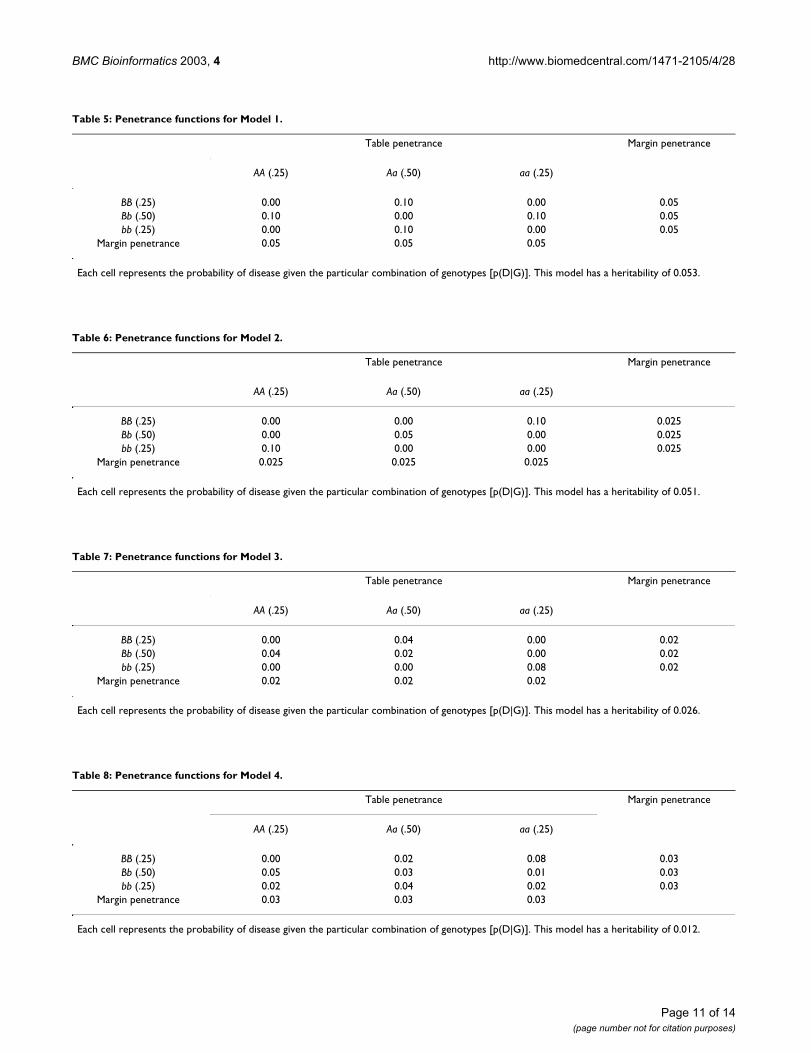
Penetrance functions model the relationship betweengenetic variations and disease risk. Penetrance is definedas the probability of disease given a particular combina-tion of genotypes. We chose five epistasis models to sim-ulate the data. The first model used was initially describedby Li and Reich [37] and later by Culverhouse et al. [34]and Moore et al. [38] (Table 5). This model is based onthe nonlinear XOR function that generates an interactioneffect in which high risk of disease is dependent oninheriting a heterozygous genotype (Aa) from one SNP ora heterozygous genotype from a second SNP (Bb), but notboth. The high-risk genotype combinations are AaBB,Aabb, AABb, and aaBb with disease penetrance of 0.1 forall four. The second model was initially described byFrankel and Schork [39] and later by Culverhouse et al.[34] and Moore et al. [38] (Table 6). In this model, highrisk of disease is dependent on inheriting two and exactlytwo high-risk alleles, either "a" or "b" from two different

Page 10 of 14(page number not for citation purposes)

BMC Bioinformatics 2003, 4 http://www.biomedcentral.com/1471-2105/4/28

Table 5: Penetrance functions for Model 1.

Table penetrance Margin penetrance

AA (.25) Aa (.50) aa (.25)

BB (.25) 0.00 0.10 0.00 0.05Bb (.50) 0.10 0.00 0.10 0.05bb (.25) 0.00 0.10 0.00 0.05

Margin penetrance 0.05 0.05 0.05

Each cell represents the probability of disease given the particular combination of genotypes [p(D|G)]. This model has a heritability of 0.053.

Table 6: Penetrance functions for Model 2.

Table penetrance Margin penetrance

AA (.25) Aa (.50) aa (.25)

BB (.25) 0.00 0.00 0.10 0.025Bb (.50) 0.00 0.05 0.00 0.025bb (.25) 0.10 0.00 0.00 0.025

Margin penetrance 0.025 0.025 0.025

Each cell represents the probability of disease given the particular combination of genotypes [p(D|G)]. This model has a heritability of 0.051.

Table 7: Penetrance functions for Model 3.

Table penetrance Margin penetrance

AA (.25) Aa (.50) aa (.25)

BB (.25) 0.00 0.04 0.00 0.02Bb (.50) 0.04 0.02 0.00 0.02bb (.25) 0.00 0.00 0.08 0.02

Margin penetrance 0.02 0.02 0.02

Each cell represents the probability of disease given the particular combination of genotypes [p(D|G)]. This model has a heritability of 0.026.

Table 8: Penetrance functions for Model 4.

Table penetrance Margin penetrance

AA (.25) Aa (.50) aa (.25)

BB (.25) 0.00 0.02 0.08 0.03Bb (.50) 0.05 0.03 0.01 0.03bb (.25) 0.02 0.04 0.02 0.03

Margin penetrance 0.03 0.03 0.03

Each cell represents the probability of disease given the particular combination of genotypes [p(D|G)]. This model has a heritability of 0.012.

Page 11 of 14(page number not for citation purposes)

BMC Bioinformatics 2003, 4 http://www.biomedcentral.com/1471-2105/4/28

loci. For this model, the high-risk genotype combinationsare AAbb, AaBb, and aaBB with disease penetrance of 0.1,0.05, and 0.1 respectively.

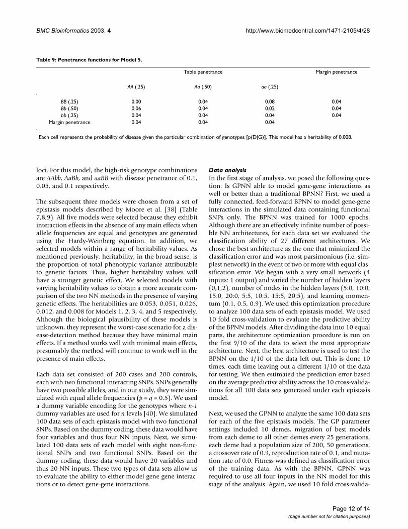
The subsequent three models were chosen from a set ofepistasis models described by Moore et al. [38] (Table7,8,9). All five models were selected because they exhibitinteraction effects in the absence of any main effects whenallele frequencies are equal and genotypes are generatedusing the Hardy-Weinberg equation. In addition, weselected models within a range of heritability values. Asmentioned previously, heritability, in the broad sense, isthe proportion of total phenotypic variance attributableto genetic factors. Thus, higher heritability values willhave a stronger genetic effect. We selected models withvarying heritability values to obtain a more accurate com-parison of the two NN methods in the presence of varyinggenetic effects. The heritabilities are 0.053, 0.051, 0.026,0.012, and 0.008 for Models 1, 2, 3, 4, and 5 respectively.Although the biological plausibility of these models isunknown, they represent the worst-case scenario for a dis-ease-detection method because they have minimal maineffects. If a method works well with minimal main effects,presumably the method will continue to work well in thepresence of main effects.

Each data set consisted of 200 cases and 200 controls,each with two functional interacting SNPs. SNPs generallyhave two possible alleles, and in our study, they were sim-ulated with equal allele frequencies (p = q = 0.5). We useda dummy variable encoding for the genotypes where n-1dummy variables are used for n levels [40]. We simulated100 data sets of each epistasis model with two functionalSNPs. Based on the dummy coding, these data would havefour variables and thus four NN inputs. Next, we simu-lated 100 data sets of each model with eight non-func-tional SNPs and two functional SNPs. Based on thedummy coding, these data would have 20 variables andthus 20 NN inputs. These two types of data sets allow usto evaluate the ability to either model gene-gene interac-tions or to detect gene-gene interactions.

Data analysisIn the first stage of analysis, we posed the following ques-tion: Is GPNN able to model gene-gene interactions aswell or better than a traditional BPNN? First, we used afully connected, feed-forward BPNN to model gene-geneinteractions in the simulated data containing functionalSNPs only. The BPNN was trained for 1000 epochs.Although there are an effectively infinite number of possi-ble NN architectures, for each data set we evaluated theclassification ability of 27 different architectures. Wechose the best architecture as the one that minimized theclassification error and was most parsimonious (i.e. sim-plest network) in the event of two or more with equal clas-sification error. We began with a very small network (4inputs: 1 output) and varied the number of hidden layers(0,1,2), number of nodes in the hidden layers (5:0, 10:0,15:0, 20:0, 5:5, 10:5, 15:5, 20:5), and learning momen-tum (0.1, 0.5, 0.9). We used this optimization procedureto analyze 100 data sets of each epistasis model. We used10 fold cross-validation to evaluate the predictive abilityof the BPNN models. After dividing the data into 10 equalparts, the architecture optimization procedure is run onthe first 9/10 of the data to select the most appropriatearchitecture. Next, the best architecture is used to test theBPNN on the 1/10 of the data left out. This is done 10times, each time leaving out a different 1/10 of the datafor testing. We then estimated the prediction error basedon the average predictive ability across the 10 cross-valida-tions for all 100 data sets generated under each epistasismodel.

Next, we used the GPNN to analyze the same 100 data setsfor each of the five epistasis models. The GP parametersettings included 10 demes, migration of best modelsfrom each deme to all other demes every 25 generations,each deme had a population size of 200, 50 generations,a crossover rate of 0.9, reproduction rate of 0.1, and muta-tion rate of 0.0. Fitness was defined as classification errorof the training data. As with the BPNN, GPNN wasrequired to use all four inputs in the NN model for thisstage of the analysis. Again, we used 10 fold cross-valida-

Table 9: Penetrance functions for Model 5.

Table penetrance Margin penetrance

AA (.25) Aa (.50) aa (.25)

BB (.25) 0.00 0.04 0.08 0.04Bb (.50) 0.06 0.04 0.02 0.04bb (.25) 0.04 0.04 0.04 0.04

Margin penetrance 0.04 0.04 0.04

Each cell represents the probability of disease given the particular combination of genotypes [p(D|G)]. This model has a heritability of 0.008.

Page 12 of 14(page number not for citation purposes)

BMC Bioinformatics 2003, 4 http://www.biomedcentral.com/1471-2105/4/28

tion to evaluate the predictive ability of the GPNN mod-els. We then estimated the prediction error of GPNNbased on the average prediction error across the 10 cross-validations for all 100 data sets for each epistasis model.

The second aspect of this study involves answering the fol-lowing question: In the presence of non-functional SNPs(i.e. potential false-positives), is GPNN able to detectgene-gene interactions as well or better than a traditionalBPNN? First we used a traditional BPNN to analyze thedata with eight non-functional SNPs and two functionalSNPs. We estimated the power of the BPNN to detect thefunctional SNPs as described below. In this network, allpossible inputs are used and the significance of each inputis calculated from its input relevance, R_I, where R_I is thesum of squared weights for the ith input divided by thesum of squared weights for all inputs. Next, we performed1000 permutations of the data to determine what inputrelevance was required to consider a SNP significant in theBPNN model. The range of critical relevance values fordetermining significance was 10.43% – 11.83%.

Next, we calculated cross-validation consistency[21,31,32]. That is, we measured the consistency withwhich each SNP was identified across the 10 cross-valida-tions. The basis for this statistic is that the functionalSNPs' effect should be present in most splits of the data.Thus, a high cross-validation consistency (~10) lends sup-port to that SNP being important for the epistasis model.Through permutation testing, we determined an empiricalcutoff for the cross-validation consistency that would notbe expected by chance. We used this cut-off value to selectthe SNPs that were functional in the epistasis model foreach data set. For the BPNN, a cross-validation consist-ency greater than or equal to five was required to be statis-tically significant. We estimated the power by calculatingthe percentage of datasets where the correct functionalSNPs were identified. Either one or both of the dummyvariables could be selected to consider a locus present inthe model. Finally, we estimated the prediction errorbased on the average predictive ability across 100 data setsfor each epistasis model.

Next, we used the GPNN to analyze 100 data sets for eachof the epistasis models. In this implementation, GPNNwas not required to use all the variables as inputs. Here,GPNN performed random variable selection in the initialpopulation of solutions. Through evolution, GPNNselects those variables that are most relevant. We calcu-lated the cross-validation consistency as described above.Permutation testing was used to determine an empiricalcut-off to select the SNPs that were functional in theepistasis model for each data set. For the GPNN, a cross-validation consistency greater than or equal to seven wasrequired to be statistically significant. We estimated the

power of GPNN as the number of times the functionalSNPs were identified in the model divided by the totalnumber of runs. Again, either one or both of the dummyvariables could be selected to consider a locus present inthe model. We also estimated the prediction error ofGPNN based on the average prediction error across 100data sets per epistasis model.

Authors' contributionsJSP, LWH, and BCW performed the computer program-ming of the software. MDR participated in the design ofthe study, statistical analyses, and writing of the manu-script. JHM participated in the design and coordination ofthe study and preparation of the final draft of the manu-script. All authors read and approved the finalmanuscript.

AcknowledgementsThis work was supported by National Institutes of Health grants HL65234, HL65962, GM31304, AG19085, AG20135, and LM007450. We would like to thank two anonymous reviewers for helpful comments and suggestions.

References1. Templeton AR: Epistasis and complex traits In: Epistasis and Evo-

lutionary Process Edited by: Wade M, Brodie III B, Wolf J. Oxford, OxfordUniversity Press; 2000.

2. Moore JH and Williams SM: New strategies for identifying gene-gene interactions in hypertension Ann Med 2002, 34:88-95.

3. Bellman R: Adaptive Control Processes Princeton, Princeton Univer-sity Press 1961.

4. Bhat A, Lucek PR and Ott J: Analysis of complex traits using neu-ral networks Genet Epidemiol 1999, 17:S503-S507.

5. Curtis D, North BV and Sham PC: Use of an artificial neural net-work to detect association between a disease and multiplemarker genotypes Ann Hum Genet 2001, 65:95-107.

6. Li W, Haghighi F and Falk C: Design of artificial neural networkand its applications to the analysis of alcoholism data GenetEpidemiol 1999, 17:S223-S228.

7. Lucek PR and Ott J: Neural network analysis of complex traitsGenet Epidemiol 1997, 14:1101-1106.

8. Lucek P, Hanke J, Reich J, Solla SA and Ott J: Multi-locus nonpara-metric linkage analysis of complex trait loci with neuralnetworks Hum Hered 1998, 48:275-284.

9. Marinov M and Weeks D: The complexity of linkage analysiswith neural networks Hum Hered 2001, 51:169-176.

10. Ott J: Neural networks and disease association studies Am JMed Genet 2001, 105:60-61.

11. Saccone NL, Downey TJ Jr, Meyer DJ, Neuman RJ and Rice JP: Map-ping genotype to phenotype for linkage analysis GenetEpidemiol 1999, 17:S703-S708.

12. Sherriff A and Ott J: Applications of neural networks for genefinding Adv Genet 2001, 42:287-298.

13. Moore JH and Parker JS: Evolutionary computation in microar-ray data analysis In: Methods of Microarray Data Analysis Edited by:Lin S, Johnson K. Boston: Kluwer Academic Publishers; 2001.

14. Koza JR and Rice JP: Genetic generation of both the weightsand architecture for a neural network IEEE Press 1991, II:.

15. Gruau FC: Cellular encoding of genetic neural networks Mas-ter's thesis Ecole Normale Superieure de Lyon 1992:1-42.

16. Moore JH, Parker JS and Hahn LW: Symbolic discriminant analy-sis for mining gene expression patterns In Lecture Notes in Artifi-cial Intelligence 2167 Edited by: De Raedt L, Flach P. Springer-Verlag,Berlin; 2001:372-381.

17. Koza JR: Genetic Programming: On the programming ofcomputers by means of natural selection Cambridge, MIT Press1993.

18. Koza JR: Genetic Programming II: Automatic discovery ofreusable programs Cambridge, MIT Press 1998.

Page 13 of 14(page number not for citation purposes)

BMC Bioinformatics 2003, 4 http://www.biomedcentral.com/1471-2105/4/28

Publish with BioMed Central and every scientist can read your work free of charge

"BioMed Central will be the most significant development for disseminating the results of biomedical research in our lifetime."

Sir Paul Nurse, Cancer Research UK

Your research papers will be:

available free of charge to the entire biomedical community

peer reviewed and published immediately upon acceptance

cited in PubMed and archived on PubMed Central

yours — you keep the copyright

Submit your manuscript here:http://www.biomedcentral.com/info/publishing_adv.asp

BioMedcentral

19. Koza JR, Bennett FH, Andre D and Keane MA: Genetic Program-ming III: Automatic programming and automatic circuitsynthesis Cambridge, MIT Press 1999.

20. Banzhaf W, Nordin P, Keller RE and Francone FE: Genetic Pro-gramming: An Introduction San Francisco, Morgan KauffmanPublishers 1998.

21. Moore JH, Parker JS, Olsen NJ and Aune TS: Symbolic discrimi-nant analysis of microarray data in autoimmune diseaseGenet Epidemiol 2002, 23:57-69.

22. Schalkoff RJ: Artificial Neural Networks, New York, McGraw-HillCompanies Inc 1997.

23. Utans J and Moody J: Selecting neural network architecturesvia the prediction risk application to corporate bond ratingprediction In: Conference Proceedings on the First International Confer-ence on Artificial Intelligence Applications on Wall Street 1991.

24. Moody J: Prediction risk and architecture selection for neuralnetworks In: From Statistics to Neural Networks: Theory and PatternRecognition Applications Edited by: Cherkassky V, Friedman JH, WechslerH. NATO ASI Series F, Springer-Verlag; 1994.

25. Fahlman SE and Lebiere C: The Cascade-Correlation LearningArchitecture Masters thesis Carnegie Mellon University School of Com-puter Science 1991.

26. Mitchell M: An Introduction to Genetic Algorithms Cambridge,MIT Press 1996.

27. Cantú-Paz E: Efficient and Accurate Parallel GeneticAlgorithms Boston, Kluwer Academic Publishers 2000.

28. Koza JR: Survey of genetic algorithms and genetic program-ming In: Wescon 95: E2. Neural-Fuzzy Technologies and Its ApplicationsIEEE, San Francisco 1995:589-594.

29. Hastie T, Tibshirani R and Friedman JH: The Elements of Statisti-cal Learning New York, Springer-Verlag 2001.

30. Ripley BD: Pattern Recognition and Neural Networks Cam-bridge, Cambridge University Press 1996.

31. Ritchie MD, Hahn LW, Roodi N, Bailey LR, Dupont WD, Parl FF andMoore JH: Multifactor dimensionality reduction reveals high-order interactions among estrogen metabolism genes insporadic breast cancer Am J Hum Genet 2001, 69:138-147.

32. Moore JH: Cross validation consistency for the assessment ofgenetic programming results in microarray studies In: LectureNotes in Computer Science 2611 Edited by: Corne D, Marchiori E. Berlin,Springer-Verlag; 2003.

33. Roland JJ: Generalisation and model selection in supervisedlearning with evolutionary computation LNCS 2003, 2611:119-130.

34. Culverhouse R, Suarez BK, Lin J and Reich T: A Perspective onEpistasis: Limits of Models Displaying No Main Effect Am JHum Genet 2002, 70:461-471.

35. Sexton RS, Dorsey RE and Johnson JD: Optimization of neuralnetworks: a comparative analysis of the genetic algorithmand simulated annealing Eur J Operat Res 1999, 114:589-601.

36. Cantú-Paz E: Evolving neural networks for the classification ofgalaxies In: Proceedings of the Genetic and Evolutionary Algorithm Con-ference Edited by: Langdon, WB, Cantu-Paz E, Mathias K, Roy R, Davis D,Poli R, Balakrishnan K, Honavar V, Rudolph G, Wegener J, Bull L, Potter MA,Schultz AC, Miller JF, Burke E, Jonoska. San Francisco, Morgan KaufmanPublishers; 2002:1019-1026.

37. Li W and Reich J: A complete enumeration and classification oftwo-locus disease models Hum Hered 2000, 50:334-349.

38. Moore JH, Hahn LW, Ritchie MD, Thornton TA and White BC:Application of genetic algorithms to the discovery of com-plex genetic models for simulations studies in human genet-ics In: Proceedings of the Genetic and Evolutionary Algorithm ConferenceEdited by: Langdon WB, Cantu-Paz E, Mathias K, Roy R, Davis D, Poli R,Balakrishnan K, Honavar V, Rudolph G, Wegener J, Bull L, Potter MA,Schultz AC, Miller JF, Burke E, Jonoska N. San Francisco, Morgan KaufmanPublishers; 2002:1150-1155.

39. Frankel WN and Schork NJ: Who's afraid of epistasis? NatureGenetics 1996, 14:371-373.

40. Ott J: Neural networks and disease association Am J Med Genet2001, 105:60-61.

Page 14 of 14(page number not for citation purposes)