Energies 2013, 6, 3422-3443; doi:10.3390/en6073422OPEN ACCESS

energiesISSN 1996-1073

www.mdpi.com/journal/energies

Article

A Power Load Distribution Algorithm to Optimize Data CenterElectrical FlowJoao Ferreira *, Gustavo Callou and Paulo Maciel

Informatics Center, Federal University of Pernambuco, Av. Jornalista Anibal Fernandes, s/n,Cidade Universitaria, Recife 50740-560, Brazil; E-Mails: grac@cin.ufpe.br (G.C.);prmm@cin.ufpe.br (P.M.)

* Author to whom correspondence should be addressed; E-Mail: jfsj3@cin.ufpe.br;Tel./Fax: +55-81-2126-8430.

Received: 13 March 2013; in revised form: 15 June 2013 / Accepted: 4 July 2013 /Published: 15 July 2013

Abstract: Energy consumption is a matter of common concern in the world today. Researchdemonstrates that as a consequence of the constantly evolving and expanding field ofinformation technology, data centers are now major consumers of electrical energy. Suchhigh electrical energy consumption emphasizes the issues of sustainability and cost. Againstthis background, the present paper proposes a power load distribution algorithm (PLDA)to optimize energy distribution of data center power infrastructures. The PLDA, which isbased on the Ford-Fulkerson algorithm, is supported by an environment called ASTRO,capable of performing the integrated evaluation of dependability, cost and sustainability.More specifically, the PLDA optimizes the flow distribution of the energy flow model(EFM). EFMs are responsible for estimating sustainability and cost issues of data centerinfrastructures without crossing the restrictions of the power capacity that each device canprovide (power system) or extract (cooling system). Additionally, a case study is presentedthat analyzed seven data center power architectures. Significant results were observed,achieving a reduction in power consumption of up to 15.5%.

Keywords: ASTRO/Mercury; energy flow model; dependability; sustainability; data centerpower architectures; power load distribution algorithm; optimization

Abbreviations:

EFM: Energy Flow Model;DAG: directed acyclic graph;

Energies 2013, 6 3423

IT: information technology;MC: Markov Chain;MTTF: mean time to fail;MTTR: mean time to repair;PLDA: Power Load Distributed Algorithm;RBD: Reliability Block Diagrams;SPN: Stochastic Petri Nets;TTF: time to fail;TTR: time to repair;UPS: uninterruptible power supplies.

1. Introduction

As a result of the development of new paradigms, such as cloud computing, e-commerce and socialnetworks, data center power consumption has increased significantly around the world in recent years(e.g., [1–3]). Large data centers are becoming critical elements in the performance of daily tasks [4].In fact, data centers now account for around 1.5% of the total power consumed in the U.S. and representa cost of $4.5 billion, a share that is expected to increase [5]. Therefore, a great deal of current research isfocused on reducing that consumption (e.g., [6–8]). On the other hand, optimization techniques appliedto saving energy have developed significantly since 2000 [9].

The conclusions of such studies are highly relevant to information technology (IT) companies whenconsidering ways to minimize operational costs and maximize sustainability [10].

Nowadays, some works aim at reducing energy consumption of data centers. Gandhi [11] performsan analysis of the effectiveness of dynamic power management in data centers. This simplest of dynamicpower management policies reduces the energy consumption by turning off servers when they arenot needed. However, the highly abstract nature of the work, which does not consider the electricalcomponents of the data center, may render the results unrealistic.

An interesting approach is presented in [12] with an integrated solution that tightly couples ITmanagement and cooling infrastructure management to improve overall efficiency of data centeroperation. Different from this work, we propose a strategy to optimize the electrical flow of data centerpower infrastructures.

In [10], the authors discuss the impact of architectural parameters on data center power consumption.The power consumption of BCube [13], DCell [14] and Fat-tree [15] data center structures is analyzed.The results show that the energy consumption of data centers, because they are designed for a muchlarger number of servers, is higher than necessary.

As opposed to previous works, what is proposed here is an optimization algorithm that would reducedata center energy consumption by improving the electrical energy flow. Additionally, the dependability,cost and sustainability issues are computed through the Energy Flow Model (EFM) and Reliability BlockDiagrams (RBD)/Stochastic Petri Nets (SPN) models supported by the ASTRO environment [16].

Energies 2013, 6 3424

This paper extends our previous work [6,17] in which an integrated approach for computingsustainability, dependability and cost issues is proposed. The main goal in this current paper is toimprove the electrical energy flow of EFM models and, as a result, improve the metrics obtainedthrough that model. The EFM [18] allows verifying if the energy flow does not exceed the maximumenergy capacity that each component can supply (considering electrical equipment) or extract (assumingcooling equipment).

Algorithms are employed to traverse the EFM in order to compute the energy consumption,sustainability impact and the operational cost of data center architectures [17]. This work proposes anew algorithm to optimize the energy flow between components by taking into account the electricalefficiency of the devices present in the EFM models. The main goal is to improve the energy flow whenthere are redundant paths available to support the demanded energy. In concise terms, the proposedalgorithm (Power Load Distributed Algorithm—PLDA) aims at increasing the utilization of those pathsthat have higher electrical efficiency levels.

It should be stressed that the EFM has the support of the ASTRO/Mercury environment [16].ASTRO is a tool that analyzes power, cooling and IT data center infrastructures. The environmentkernel, Mercury, is responsible for performing the evaluation of the supported models (Stochastic Petrinets—SPN; Reliability Block Diagrams—RBD; EFM; and Markov Chain—MC) [19]. ASTRO providesviews for modeling data center power, cooling and IT infrastructures from which non-specializedusers may conduct the dependability, sustainability and cost evaluation without the need to be familiarwith those formalisms used by Mercury [16]. Models created through the ASTRO environment areautomatically converted to models supported by Mercury (for the dependability evaluation).

A case study is conducted to compare the dependability, sustainability and cost results obtainedbefore and after applying the optimization technique (PLDA algorithm) to different data center powerarchitectures. The computed dependability evaluation employs a hierarchical approach that recognizesthe advantages of both stochastic Petri nets (SPN) [20] and Reliability Block Diagrams (RBD) [21].

The paper is organized as follows: Section 2 introduces basic concepts regarding data centerinfrastructures, sustainability, directed acyclic graphs (DAGs) and dependability; Section 3 presents anoverview of Reliability Block Diagram (RBD); Section 4 presents an overview of the ASTRO/Mercuryenvironment; Section 5 describes the Energy Flow Model (EFM); Section 6 explains the PLDA;Section 7 applies the adopted methodology; Section 8 presents a real-world case study; and finally,Section 9 concludes the paper and suggests directions for future work.

2. Preliminaries

This section discusses the basic concepts needed for a better understanding of the paper and presentsan overview of data center infrastructures, followed by an explanation of the concepts of exergy anddirected acyclic graphs. Finally, the concepts about dependability are introduced.

2.1. Data Center

With the aim of ensuring availability, a data center is the concentration in one location of theprocessing and data storage devices responsible for running the business of organizations. Power outages

Energies 2013, 6 3425

and electrical energy oscillations are important events that a data center must be able to deal with in orderto avoid damage to its equipment and provide the high availability demanded. A data center essentiallyconsists of three sub-systems:

• The IT infrastructure comprises three main components: servers, network equipment and storagedevices. Software services are usually organized in a multi-tier architecture with separate layersfor web-servers, application servers and databases.

• The cooling infrastructure is responsible for extracting heat from the data center room. Itaccounts for between 10% and 20% of the total data center energy consumption [22].

• The power infrastructure provides uninterrupted and conditioned electrical energy at the correctvoltage and frequency to the IT and cooling sub-systems. The electricity passes throughtransformers, transfer switches, uninterruptible power supplies (UPS), distribution boards and,finally, to rack power strips [23]. The current work focuses on the power infrastructure.

2.2. Exergy

There are several interconnected methods of comparing equipment from the point of view ofsustainability, for example: respective electrical energy consumption; the materials used in manufacture;or the environmental impact and irreversible environmental losses for future generations. Thesealternative techniques for measuring sustainability occasionally produce conflicting results. For instance,any particular item of equipment may be considered a better option than another, if despite having higherpower consumption, it has a positive impact on the future environment.

Exergy is a metric that estimates the energy consumption efficiency of a system, such as thearchitecture of a data center. As an index for the global assessment of sustainability, the thermodynamicproperty of exergy is of great importance. It is defined as the maximal fraction of latent energy that canbe theoretically converted into useful work [24]. A useful illustration would be to compare the exergy of1 kJ of gasoline with that of 1 kJ of water at ambient temperature. The exergy of the gasoline is muchgreater, since it can be used to move a truck, but the water at ambient temperature cannot.

2.3. Directed Acyclic Graph

A graph can be described as a structure constituted by two elements: the arcs and vertices.In recent decades, a relationship between algorithms and graphs has been studied. In general, the area ofalgorithms and graphs may be characterized as one whose primary interest is to solve problems in graphsusing algorithms, keeping in mind a computing concern. In this study, the case is repeated once we havea problem in a graph. There are several types of graphs with several special issues (e.g., complete,symmetric, cyclic, directed, etc.) [25]. This paper adopts directed acyclic graphs.

A directed graph, D (V,E), is a finite nonempty set, V (vertices), and a set of arcs, E (edges) orderedpairs of distinct vertices [26]. Thus, in a directed graph, each arc (v,w) has only one direction from v to w.In an acyclic graph, the initial and final vertices cannot be the same for any subpath in the graph.

In this paper, the EFM is a directed acyclic graph. For more details about the graphs, the reader isredirected to [25,26].

Energies 2013, 6 3426

2.4. Dependability

The dependability of a system can be understood as the ability to deliver a set of services that can bejustifiably trusted [21,27,28]. In point of fact, dependability is closely related to the concepts of faulttolerance and reliability.

Reliability is the probability that the system will deliver a set of services for a given period oftime. Fault tolerance is the ability of a system not to fail even when there are faulty components [29].In fault-tolerant systems, the reliability provides the probability that a system will function even whenthere are faulty components.

Availability is another important concept that quantifies the mixed effect of both the failure and repairprocess in a system [21]. To calculate the availability value of a given device or system, the uptimeand the downtime, or the time to failure (TTF) and time to repair (TTR), need to be known. Since thespecific uptime and downtime are not accessible, the solution is to use mean values. In such a situation,the commonly adopted metrics are mean time to failure (MTTF) and mean time to repair (MTTR).For more details, the reader should refer to [21], which also supplies the equations for estimatingdependability metrics.

3. Dependability Model—Reliability Block Diagram

The Reliability Block Diagram (RBD) is a combinatorial model that was initially proposed as atechnique for calculating the reliability of systems by employing intuitive block diagrams. The techniquewas then extended to compute availability and maintainability [21].

The RBD structure establishes a logical interaction between the components, defining whichcombinations of failed and active elements are able to sustain system operation. Thus, the systemis represented by subsystems or components connected according to their function or reliabilityrelationship [30].

Figure 1a is an illustration of a series arrangement, where the failure of a single component will causethe whole system to cease to function [31].

Assuming a system with n independent components, the reliability (instantaneous availability orsteady state availability) is calculated by:

Ps =n∏i=1

Pi (1)

where Pi is the reliability—Ri(t) (instantaneous availability (Ai(t)) or steady state availability (Ai))—ofblock bi.

Figure 1b depicts a parallel arrangement, where the whole system will continue to function, even ifonly a single component is operational [31].

Assuming a system with n independent components, the reliability (instantaneous availability orsteady state availability) is calculated by:

Pp = 1−n∏i=1

(1− Pi) (2)

Energies 2013, 6 3427

Figure 1. (a) Serial arrangement; and (b) parallel configuration.

A k-out-of-n system functions if and only if k or more of its n components are functioning. LetPi be the success probability of each of those blocks. The system success probability (reliability oravailability) is calculated by:

Σni=k

(n

i

)P k(1− P )n−k (3)

For other examples and closed-form equations, the reader should refer to [21].

3.1. Structure Function

Structural functions are used to represent the relationship between the individual components andsystem state. Consider a system, S, composed by a set of components, C = ci | 1 ≤ i ≤ n, where thestate of the system, S, and its components could be either operational or failed and n is the number ofcomponents of the system. Let the discrete random variable, xi, indicate the state of component i; thus:

xi =

0−if the component i has failed

1−if the component i is operational(4)

Additionally, a vector, x = (x1, x2, ..., xn), represents the state of each component of the system.The state of the system is determined by the states of the components. The structure function, φ(x),maps the system state vector, x, to one or zero, as shown below:

φ(x) =

0−if the system has failed

1−if the system is operational(5)

The blocks (e.g., components) are usually arranged using the following composition mechanisms:series, parallel, k-out-of-n blocks, bridge or even a combination of previous approaches. The followinglines highlight the structural and parallel composition utilized in this paper.

Serial Components: Let n components, x1, x2, ..., xn, in series; the structural function of thesecomponents is represented by:

φ(x) = min(x1, x2, ..., xn)

φ(x) =n∏i=1

xi(6)

Energies 2013, 6 3428

Parallel System: Let n components, x1, x2, ..., xn, in parallel; the structural function of thesecomponents is represented by:

φ(x) = max(x1, x2, ..., xn)

φ(x) = 1−n∏i=1

(1− xi)(7)

3.2. Logic Function

Logical functions have the same goal of structural functions: to indicate a relationship between thestates of the components and the state of the system. However, in some cases, simplifying the structurefunction may not be an easy task [21]. A logic function of a coherent system may be adopted to simplifythe system’s functions through Boolean algebra.

Serial Components: Let x = (x1, x2, ..., xn), the vector that represents the state of n components ofa system. The serial logic function (S) is defined by:

Sserial(x) = (x1 ∧ x2 ∧ ... ∧ xn)

Parallel System: Let x = (x1, x2, ..., xn), the vector that represents the state of n components of asystem. The parallel logic function (S) is defined by:

Sparallel(x) = (x1 ∨ x2 ∨ ... ∨ xn)

For more details about structured or logic functions, the reader is redirected to [21,32].

4. ASTRO/Mercury Environment

ASTRO is a tool that analyzes power, cooling and IT data center and cloud infrastructures [16].The environment’s kernel, named Mercury, is responsible for evaluating the supported models:Stochastic Petri Nets (SPN), Reliability Block Diagrams (RBD), EFM and Markov Chain (MC). Mercurysupports the difficulties encountered with RBD modeling (e.g., dependency relationship), which may besolved by SPN or MC.

Figure 2 presents the relation between ASTRO and Mercury. It is important to state that the modelbuilt through the IT, power and cooling views available in ASTRO can be automatically converted to themodels supported by Mercury (for dependability evaluation).

Therefore, in the ASTRO environment, non-specialized users may conduct the dependability,sustainability and cost evaluations without the need to be familiar with those models. This work focuseson the Mercury environment.

Figure 3 depicts the Mercury environment. The highlighted rectangle shows the set of modelsavailable in the Mercury tool. In this figure, an example of the EFM is also depicted.

In the ASTRO/Mercury environment, non-specialized users may conduct the dependability,sustainability and cost evaluations without the need to be familiar with those models.

For more details about the ASTRO/Mercury tool, the reader is redirected to [16].

Energies 2013, 6 3429

Figure 2. Environment functionalities.

Figure 3. Mercury environment.

5. Energy Flow Model

The Energy Flow Model (EFM) [18] quantifies the energy flow between system components, whilstrespecting the maximum energy that each component can provide or extract. The EFM is representedby a directed acyclic graph in which components are modeled as vertices and the respective connectionscorrespond to edges. The following defines the EFM: G = (N,A,w, fd, fc, fp, fη), where:

• N = Ns ∪ Ni ∪ Nt represents the set of nodes (i.e., the components), in which Ns is the set ofsource nodes, Nt is the set of target nodes and Ni denotes the set of internal nodes, Ns ∩ Ni =

Ns ∩Nt = Ni ∩Nt = �;

• A ⊆(Ns × Ni) ∪ (Ni × Nt) ∪ (Ni × Ni) = {(a,b) | a 6= b} denotes the set of edges (i.e., thecomponent connections).

Energies 2013, 6 3430

• w : A → R+ is a function that assigns weights to the edges (the value assigned to the edge (j, k)is adopted for distributing the energy assigned to the node, j, to the node, k, according to the ratio,w(j,k)/

∑i∈j• w(j, i), where j• is the set of output nodes of j);

• fd : N →

R+ if n ∈ Ns ∪Nt,

0 otherwise;

is a function that assigns to each node the heat to be extracted (considering cooling models) or theenergy to be supplied (regarding power models);

• fc : N →

0 if n ∈ Ns ∪Nt,

R+ otherwise;

is a function that assigns each node with the respective maximum energy capacity;

• fp : N →

0 if n ∈ Ns ∪Nt,

R+ otherwise;

is a function that assigns each node (a node represents a component) with its retail price;

• fη : N →

1 if n ∈ Ns ∪Nt,

0 ≤ k ≤ 1, k ∈ R otherwise;

is a function that assigns each node with the energetic efficiency.

For more details about EFM modeling, the reader is directed to [18].

Example

Figure 4 is an example of an EFM. The rounded rectangles equate to the type of equipment, andthe labels name each item. The edges have weights that are used to direct the energy flow betweenthe components. For the sake of simplicity, the graphical representation of EFM models hides thedefault weight, one.

In the present paper, the EFM is employed to compute the overall energy required to provide thenecessary energy at the target point. The demanded power associated to TargetPoint1 is 128.25 kW. Thus,since the efficiency of STS1 (Static Transfer Switch) is 95%, the electrical power the STS componentmust receive is 135 kW.

A similar strategy is adopted for component, UPS1. Since its energy efficiency is 90%, the electricalpower flowing through it is 150 kW. From UPS1, the flow is divided between the two AC sourcesaccording to the associated edge weights. Therefore, 120 kW of the flow is assigned to ACSource1and 30 kW to the other. The process continues until SourcePoint1 is reached, which accumulates thetotal flow.

However, here, the respective weights and efficiency of the ACSource components do not correspond.A weight of 0.8 units is ascribed to the edge that connects the UPS node to ACSource1 and a weight of0.2 to the other edge that connects the node to ACSource2. This means that ACSource1 supplies fourtimes more power than ACSource2.

Energies 2013, 6 3431

It is important to stress that the edge weights are defined by the model designer. There is no guaranteethat the designers allocate the best values for that distribution, and the outcome may be higher powerconsumption. The present paper aims to optimize the edge weight distribution of the EFM model througha Power Load Distribution Algorithm, as explained in Section 6.

Figure 4. A simple example of energy modeling with the Energy Flow Model (EFM).

5.1. Cost

The evaluated capacity of cost in a data center is essential for an analysis of return on investment andother business decision processes. This work considers acquisition and operational costs. The acquisitioncost is the financial resource required to purchase the data center infrastructure. The operational costcorresponds to the cost of the operation of the data center for a period of time, considering energyconsumed, energy cost, period of evaluation and the availability of the data center.

In this paper, the operational cost is utilized as a metric to financial evaluation of the data center, oncethis metric relates availability and energy consumption. It is computed by the following Equation (8).In addition, it is important to stress that other costs (e.g., maintenance cost) can be added to this equation.

OpCost = PInput × CEnergy × T × (A+ α(1− A)) (8)

where: OpCost is the operational cost; Pinput is the electrical energy consumed; Cenergy is the energycost; T is the assumed period; A is the availability; and α is the factor adopted to represent the amountof energy that continues to be consumed when a component has failed.

5.2. Operational Exergy

In this work, the operational exergy is used to measure the environmental impact of the electricalenergy waste of the electrical components of the data center. Each electrical component dissipates afraction of heat, which is not theoretically converted into useful work, called operational exergy.

The lower the value of operational exergy, the lower the environmental impact from the data centerinfrastructure. Equation (9) is used to compute the value of operational exergy:

Exop =n∑i=1

Exopi × T × (A+ α(1− A)) (9)

Energies 2013, 6 3432

where Exopi is the operational exergy of each device; T is the period of analysis; A is the systemavailability; and α is the factor that represents the amount of energy that continues to be consumed aftera component has failed.

Each type of device uses a specific equation to calculate the operational exergy. The equation used toevaluate a diesel generator is different from that used to evaluate a cooling tower. This study consideredonly electrical devices, and Equation (10) is utilized to compute the exergy of each device.

Pin × (1− η) (10)

where: Pin is the total input power of the electrical device; and η is the delivery efficiency.For more information, the reader is redirected to [17].

6. Power Load Distribution Algorithm

A Power Load Distribution Algorithm (PLDA) is proposed to minimize the electrical energyconsumption of the EFM models [18]. The PLDA is based on the Ford-Fulkerson algorithm, whichcomputes the maximum possible flow in a flow network [33]. The network is represented by a graph,where the transport capacity of the devices is defined in the edges. The algorithm begins by traversingthe graph, searching for the best flows between two specific points in the graph. If a particular pathlacks the capacity to support all of the flow demanded, then the residual flow is redirected to other paths.The Priority First Search (PFS) is the adopted method for selecting the path between the nodes. ThePFS chooses the path according to the highest electrical capacities of nodes in the graph [34]. For moredetails about the Ford-Fulkerson algorithm, the reader is referred to [33].

The flow to be distributed (called demanded electrical energy) is an element of the EFM model.The demand is inserted into the destination vertex and will be the stop criterion of the algorithm. Whilstthere is demanded energy in the destination vertex, a “path” is sought to transmit that flow. The choiceis made from among the vertices belonging to that path and is the vertex with the lowest capacity.

After each iteration, the value of the aforementioned lowest capacity vertex is subtracted from thedemanded value. For every vertex of that path, the flow is increased and the capacity decremented bythe value of the transmitted flow. All changes are applied to the EFM model.

The PLDA algorithm is composed of two functions, initialize and PLDA. Algorithm 1 (functionInitialize) is responsible for initializing variables, as well as performing calls to the PLDA. The number ofcalls corresponds to the number of target nodes on the EFM model, G, set as a parameter in Algorithm 1.The first step of the algorithm is to make a copy of the original graph, G. The copy is stored in thevariable, R (Line 1). A vector, named ccu, is employed to associate to each node a value that expressesthe current capacity utilized by each node. Line 3 initializes the ccu of each node to zero. Next, arepetition structure (Lines 5 to 7) is adopted to perform calls to the PLDA kernel. Finally, the weightson the edges of the EFM model are updated according to the current accumulated vector, ccu (Line 8).

The function PLDA (Algorithm 2) is the kernel of the power load distribution algorithm. Algorithm 2begins by checking if there is a valid path from the node, n, to the node, s. The n is an element of the setof target nodes, Nt, and the s is an element of the set of source nodes, Ns, of the EFM. A valid path is apath from one node to another where the electrical capacity of all components in this path are respected.The variable, P , is a vector that holds the elements of a valid path (line 2). Once a valid path is verified,

Energies 2013, 6 3433

a symbol representing infinity is assigned to the variable, pf (line 3). In Line 5, pf receives the valuereturned by the call to the function, getMinimumCapacity(). This function is responsible for computingthe minimum capacity of the paths available. Next, the ccu of each node is updated (Line 8). In addition,the demanded electrical power of the node, n, is also updated (Line 10). The previous steps are repeateduntil all valid paths have been analyzed. Finally, the residual graph, R, is returned. It is important tostress that only the edge weights are changed from the original graph, G.

Algorithm 1 Initialize Power Load Distribution Algorithm (PLDA; G)1: R = G;2: for i ∈ N do3: ccui = 0;

4: end for5: for n ∈ Nt do6: R = PLDA(R, fd(n), n);

7: end for8: setUpdateWeight(R);

9: return R;

Algorithm 2 PLDA (R, fd(n), n)1: while (isPathValid(R,n,s)) & (fd(n) > 0) do2: P = getElementsFromV alidPath(R,n, s);

3: pf =∞;

4: for i ∈ P do5: pf = getMinimumCapacity(pf, fc(i) − ccu(i));

6: end for7: for i ∈ P do8: ccui = ccui + pf ;

9: end for10: fd(n) = fd(n) - pf ;11: end while12: return R

Example

Figure 5 illustrates the EFM model of a specified architecture. In the example, all the edge weightsare set to the default value, one. The power flow is computed by traversing the graph from the target tothe source node.

Figure 6 depicts the EFM model after the execution of the PLDA. It should be noted that the weightson the edges have changed, optimizing the power flow through a best weights distribution.

Table 1 presents a summary of the results obtained by the PLDA. Column “Improvement” depictsthe improvement. The system efficiency is improved by over 4.2%; consequently, the associated costand sustainability figures are improved by 4.2% and 20.4%, respectively. Availability results were alsocomputed with RBD/SPN models, but are not included here.

Energies 2013, 6 3434

Figure 5. EFM model.

Figure 6. EFM model after PLDA execution.

Table 1. Summary results before and after PLDA execution.

Metric Before After Improvement (%)

Availability (%) 0.99999226 0.99999226 0Number of 9 s 5.111 5.111 0Downtime (hs) 0.0677 0.0677 0Input Power (kW) 1,312.63 1,259.64 4.2System Efficiency (%) 76.18 79.38 4.2Operational Cost (USD) 1,264,849 1,213,784 4.2Operational Exergy (GJ) 9,859.32 8,188.11 20.4

7. Methodology

Figure 7 depicts an overview of the allocation methodology. Its first step comprises understandingthe system components, interfaces and interactions. This phase should also produce the set of metrics(e.g., input power, availability, reliability, costs) to be evaluated. The next stage is to create the high-levelmodels that represent the data center architecture. These high-level models can be created by adoptingthe data center views present in the ASTRO tool. The dependability models can be automaticallyobtained by the models created in ASTRO. Besides, the EFM is also generated.

Energies 2013, 6 3435

Figure 7. Methodology.

The PLDA optimizes the energy flow distribution of the EFM models, which are available in theMercury tool. Therefore, following the adopted methodology, at this time, there are two ways to proceed,the application or not of the PLDA algorithm. If it is executed, then, the algorithm updates the EFMmodel with different weights on the edges. This optimizes the electrical energy flow distribution ofEFM. The next stage is to conduct the evaluation of the dependability model, which is followed by theevaluation of the EFM and takes into account the availability result obtained through the dependabilityevaluation. Finally, the evaluation results are obtained.

In order to show the applicability of the PLDA algorithm, the results obtained considering theexecution of PLDA may be compared with the results from the models that were not optimized.Such comparison is further performed in Section 8.

8. Case Study

The objective of the case study was to verify the applicability of the PLDA. Seven data centerpower infrastructures were evaluated (see Figure 8). For each architecture, the following metrics werecalculated: (i) operational exergy; (ii) operational cost; (iii) availability; (iv) number of nines (availabilityin another view); (v) downtime (year); (vi) input power; and (vii) system efficiency.

Energies 2013, 6 3436

Figure 8. Architectures A1 to A7.

Energies 2013, 6 3437

These values were computed over the period of one year. Each metric was computed before and afterthe PLDA execution.

8.1. Architectures

The architectures analyzed are similar to those present in HP Labls, Palo Alto, CA, USA [35].Beginning from the real power infrastructure depicted in Figure 8 (A1), the other architectures weredefined according to the reliability importance index [23]. This index identifies the component to bereplicated. For instance, in architecture A1, component, ACSource, was indicated to be replicated.Therefore, A2 corresponds to A1 considering component, ACSource, replicated. A similar approachwas adopted to propose the other architectures. Typically, the electrical flow in a data center starts froma power supply (i.e., AC source) and, then, passes through voltage panels, uninterruptible power supplyunits (UPSs), power distribution units (PDUs) (composed of a transformer and an electrical subpanel),junction boxes and, finally, to rack PDUs (rack power distribution units). As detailed in Table 2, the casestudy employs redundant devices with dissimilar electrical efficiencies. The table also lists the maximumenergy capacity of each device.

Table 2. Capacity and efficiency.

Equipment Efficiency (%) Capacity (kW)

AC Source 1 95.3 10,000AC Source 2 90 10,000STS 1 99.5 1,500STS 2 98 1,500STS 3 99.5 1,500SDT (or Transformer) 1 98.5 5,000SDT (or Transformer) 2 95 5,000Sub Panel 1 99.9 1,500Sub Panel 2 95 1,500Sub Panel 3 99.9 1,500Low Voltage Panel 1 99.9 1,500Low Voltage Panel 2 95 1,500UPS 1 95.3 5,000UPS 2 90 5,000Junction Box 1 99.9 1,500Junction Box 2 98 1,500Power Strip 95.1 5,000

8.2. Models

This section presents the models for A5. However, a similar process was followed to evaluate theother architectures (A1–A4, A6 and A7). Figure 9 illustrates the RBD model for architecture A5.

Energies 2013, 6 3438

Figure 9. Reliability Block Diagram (RBD) model of architecture A5.

The evaluation of the RBD model provides the availability metric. This is achieved by followingthese functions.

Logic Function:

Ψ(S) = ((ACS1) ∨ (ACS2)) ∧ (STS1) ∧ (LV P1) ∧ (((UPS1) ∧ (T1)) ∨ ((UPS2)

∧(T2))) ∧ (STS3) ∧ (SP1) ∧ ((JB1) ∨ (JB2)) ∧ (RPDU1) ∧ ((RPDU2)

∧(RPDU3)) ∧ (RPDU4) ∨ (RPDU5)

(11)

Structural Function:

Φ(X) = (1− (1− ACS1)× (1− ACS2))× (STS1)× (LV P1)× (1− (1− (UPS1)

×(1− (UPS2)× (T2)))× (STS3)× (SP1)× (1− (1− JB1)× (1− JB2))

×(RPDU1)× ((RPDU2)× (RPDU3))× (RPDU4)× (RPDU5)

(12)

Availability Function:

A = P{Φ(X) = 1} = E{(1− (1− ACS1)× (1− ACS2))× (STS1)× (LV P1)

×(1− (1− (UPS1)× (T1))× (1− (UPS2)× (T2)))× (STS3)

×(SP1)× (1− (1− JB1)× (1− JB2))× (RPDU1)

×((RPDU2)× (RPDU3))× (RPDU4)× (RPDU5)}

(13)

Table 3 depicts the variables used in Functions (11)–(13), their respective equipment and definitions.For more details about the notation of variables and procedures, the reader is referred to [32]. The MTTFand MTTR values needed to compute the availability were obtained from [36].

Table 3. Equipment, associated variables and definitions.

Equipment Variables Definition

AC Source 1 and 2 AC S1 and AC S2 AC SourceSTS 1 and 3 STS1 and STS3 Static Transfer SwitchSub Panel 1 SP1 Sub PanelLow Voltage Panel 1 LVP1 Low Voltage PanelUPS 1 and 2 UPS1 and UPS2 Uninterruptible Power SupplyJunction Box 1 and 2 JB1 and JB2 Junction BoxPower Strip RPDU(1..5) Power Strip

Energies 2013, 6 3439

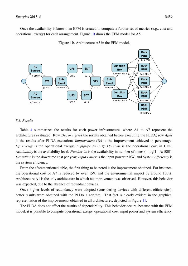
Once the availability is known, an EFM is created to compute a further set of metrics (e.g., cost andoperational exergy) for each arrangement. Figure 10 shows the EFM model for A5.

Figure 10. Architecture A5 in the EFM model.

8.3. Results

Table 4 summarizes the results for each power infrastructure, where A1 to A7 represent thearchitectures evaluated. Row Before gives the results obtained before executing the PLDA; row Afteris the results after PLDA execution; Improvement (%) is the improvement achieved in percentage;Op Exergy is the operational exergy in gigajoules (GJ); Op Cost is the operational cost in UDS;Availability is the availability level; Number 9s is the availability in number of nines (−log[1−A/100]);Downtime is the downtime cost per year; Input Power is the input power in kW; and System Efficiency isthe system efficiency.

From the aforementioned table, the first thing to be noted is the improvement obtained. For instance,the operational cost of A7 is reduced by over 15% and the environmental impact by around 100%.Architecture A1 is the only architecture in which no improvement was observed. However, this behaviorwas expected, due to the absence of redundant devices.

Once higher levels of redundancy were adopted (considering devices with different efficiencies),better results were obtained with the PLDA algorithm. That fact is clearly evident in the graphicalrepresentation of the improvements obtained in all architectures, depicted in Figure 11.

The PLDA does not affect the results of dependability. This behavior occurs, because with the EFMmodel, it is possible to compute operational exergy, operational cost, input power and system efficiency.

Energies 2013, 6 3440

Table 4. Results of PLDA execution with improvement in %.

Architectures - Op Exergy Op Cost (USD) Availability Number 9s Downtime (year) Input Power System Efficiency (%)

A1

Before 5,627 1,133,569 0.9979 2.684 18.121 1,178.82 84.82

After 5,627 1,133,569 0.9979 2.684 18.121 1,178.82 84.82

Improvement (%) 0 0 0 0 0 0 0

A2

Before 6,922 1,174,589 0.9994 3.255 4.8667 1,219.63 81.99

After 5,823 1,140,993 0.9994 3.255 4.8667 1,184.75 84.4

Improvement (%) 18.8 2.9 0 0 0 2.9 2.9

A3

Before 8,253 1,215,242 0.99943 3.25 4.92 1,261 79.24

After 6,010 1,146,719 0.99943 3.25 4.92 1,190 83.98

Improvement (%) 37.3 5.9 0 0 0 5.9 5.9

A4

Before 9,005 1,238,130 0.9993 3.171 5.902 1,285 77.77

After 6,010 1,146,591 0.9993 3.171 5.902 1,190 83.98

Improvement (%) 49.8 7.9 0 0 0 7.9 7.9

A5

Before 9,398 1,250,134 0.9993 3.172 5.8887 1,298 77.02

After 6,010 1,146,592 0.9993 3.172 5.8887 1,190 83.98

Improvement (%) 56 9 0 0 0 9 9

A6

Before 10,383 1,280,685 0.9997 3.698 1.7547 1,329 75.22

After 5,825 1,141,398 0.9997 3.698 1.7547 1,184 84.4

Improvement (%) 78.2 12.2 0 0 0 12.2 12.2

A7

Before 11,410 1,312,259 0.9999 5.11 0.067 1,361.84 73.43

After 5,639 1,135,910 0.9999 5.11 0.067 1,178 84.83

Improvement (%) 102 15.5 0 0 0 15.5 15.5

Figure 11. Comparison before and after PLDA execution.

9. Conclusions

The present paper proposed an algorithm, called the Power Load Distribution Algorithm (PLDA),to reduce the electrical energy consumption of data center power infrastructures. The main goal of thePLDA algorithm is to automatically allocate more appropriate values to the edge weights of the EFMmodels. Such an optimization-based approach was evaluated through a case study, which demonstratedthat the results obtained after the execution of the PLDA were significantly better. For some of the casestudy architectures, the results for sustainability impact (exergy) were improved by more than 100%, and

Energies 2013, 6 3441

power consumption, system efficiency and operational cost were improved by up to 15%. In the worstcase, the results were equal to those obtained without the PLDA.

In the future, we intend to study how dynamic power management can help to optimize data centerelectrical consumption.

Acknowledgments

The authors would like to thank the reviewers for their valuable comments and suggestions to improvethe quality of this work.

Conflict of Interest

The authors declare no conflict of interest.

References

1. U.S. Environmental Protection Agency (U.S. EPA). Report to Congress on Server andData Center Energy Efficiency; U.S. EPA: Washington, DC, USA, 2007. Availableonline: http://www.energystar.gov/ia/partners/prod development/downloads/EPA Datacenter Re-port Congress Final1.pdf (accessed on 11 July 2013).

2. Abbasi, Z.; Varsamopoulos, G.; Gupta, S. Thermal Aware Server Provisioning and WorkloadDistribution for Internet Data Centers. In Proceedings of ACM International Symposium onHigh Performance Distributed Computing (HPDC10), Chicago, IL, USA, 20–25 June 2010;pp. 130–141.

3. Al-Qawasmeh, A. Heterogeneous Computing Environment Characterization and Thermal-AwareScheduling Strategiesto Optimize Data Center Power Consumption. Ph.D. Thesis, Colorado StateUniversity, Collins, CO, USA, 2012.

4. Gil Montoya, F.; Manzano-Agugliaro, F.; Gomez Lopez, J.; Sanchez Alguacil, P. Power qualityresearch techiniques: Advantages and disadvantages. DYNA 2012, 79, 66–74.

5. Bouley, D. Estimating a Data Centers Electrical Carbon Footprint; White Paper66; APC by Schneider Electric: West Kingston, RI, USA, 2011. Availableonline: http://www.apc-by-schneider.de/ whitepapers/docs/066%20-%20Estimating%20a%20Data%20Center’s%20Electrical%20Carbon%20Footprint.pdf (accessed on 11 July 2013).

6. Callou, G.; Sousa, E.; Maciel.; Magnani, F. A Formal Approach to the Quantification ofSustainability and Dependability Metrics on Data Center Infrastructures. In Proceedings ofDEVS—Discrete Event System Specification, Boston, MA, USA, 3–7 April 2011; pp. 274–281.

7. Gmach, D.; Chen, Y.; Shah, A.; Rolia, J.; Bash, C.; Christian, T.; Sharma, R. ProfilingSustainability of Data Centers. In Proceedings of 2010 IEEE International Symposium onSustainable Systems and Technology (ISSST), Arlington, VA, USA, 17–19 May 2010; pp. 1–6.

8. Zhang, X.; Zhao, X.; Li, Y.; Zeng, L. Key Technologies for Green Data Center. In Proceedingsof 2010 3rd International Symposium on Information Processing (ISIP), Qingdao, China, 15–17October 2010; pp. 477–480.

Energies 2013, 6 3442

9. Banos, R.; Manzano-Agugliaro, F.; Montoya, F.; Gil, C.; Alcayde, A.; Gomez, J. Optimizationmethods applied to renewable and sustainable energy: A review. Renew. Sustain. Energy Rev.2011, 15, 1753–1766.

10. Gyarmati, L.; Trinh, T. How Can Architecture Help to Reduce Energy Consumption in Data CenterNetworking? In Proceedings of the 1st International Conference on Energy-Efficient Computingand Networking, Passau, Germany, 13–15 April 2010; ACM: New York, NY, USA, 2010;pp. 183–186.

11. Gandhi, A.; Harchol-Balter, M. How Data Center Size Impacts the Effectiveness of Dynamic PowerManagement. In Proceedings of 2011 IEEE 49th Annual Allerton Conference on Communication,Control, and Computing (Allerton), Monticello, IL, USA, 28–30 September 2011; pp. 1164–1169.

12. Chen, Y.; Gmach, D.; Hyser, C.; Wang, Z.; Bash, C.; Hoover, C.; Singhal, S. IntegratedManagement of Application Performance, Power and Cooling in Data Centers. In Proceedingsof 2010 IEEE Network Operations and Management Symposium (NOMS), Osaka, Japan, 19–23April 2010; pp. 615–622.

13. Guo, C.; Lu, G.; Li, D.; Wu, H.; Zhang, X.; Shi, Y.; Tian, C.; Zhang, Y.; Lu, S. BCube: Ahigh performance, server-centric network architecture for modular data centers. ACM SIGCOMMComput. Commun. Rev. 2009, 39, 63–74.

14. Guo, C.; Wu, H.; Tan, K.; Shi, L.; Zhang, Y.; Lu, S. Dcell: A scalable and fault-tolerant networkstructure for data centers. ACM SIGCOMM Comput. Commun. Rev. 2008, 38, 75–86.

15. Greenberg, A.; Hamilton, J.; Jain, N.; Kandula, S.; Kim, C.; Lahiri, P.; Maltz, D.; Patel, P.;Sengupta, S. VL2: A scalable and flexible data center network. ACM SIGCOMM Comput.Commun. Rev. 2009, 39, 51–62.

16. Silva, B.; Callou, G.; Tavares, E.; Maciel, P.; Figueiredo, J.; Sousa, E.; Araujo, C.; Magnani, F.;Neves, F. ASTRO: An integrated environment for dependability and sustainability evaluation.Sustain. Comput. Inform. Syst. 2012, 3, 1–17.

17. Callou, G.; Maciel, P.; Tutsch, D.; Ferreira, J.; Arajo, J.; Souza, R. Estimating sustainability impactof high dependable data centers: A comparative study between Brazilian and U.S. energy mixes.Computing 2013, doi:10.1007/s00607-013-0328-y.

18. Callou, G.; Maciel, P.; Tutsch, D.; Araujo, J. Models for Dependability and Sustainability Analysisof Data Center Cooling Architectures. In Proceedings of 2012 IEEE International Conference onDependable Systems and Networks (DSN), Boston, MA, USA, 25–28 June 2012; pp. 1 –6.

19. Ciardo, G.; Blakemore, A.; Chimento, P.F.; Muppala, J.K.; Trivedi, K.S. Automated Generationand Analysis of Markov Reward Models Using Stochastic Reward Nets. In Linear Algebra, MarkovChains, and Queueing Models; IMA Volumes in Mathematics and its Applications; Springer:New York, NY, USA, 1993; Volume 48, p. 145.

20. Trivedi, K. Probability and Statistics with Reliability, Queueing, and Computer ScienceApplications, 2nd ed.; Wiley Interscience Publication: New York, NY, USA, 2002.

21. Kuo, W.; Zuo, M.J. Optimal Reliability Modeling—Principles and Applications; Wiley: Hoboken,NJ, USA, 2003.

Energies 2013, 6 3443

22. Rasmussen, N. An Improved Architecture for High-Efficiency, High-Density Data Centers; WhitePaper 126; APC by Schneider Electric: West Kingston, RI, USA, 2008. Available online:http://www.getitgreenohio.info/documents/White%20Paper%20126%20-%20High-Efficiency%20Architecture%20(2).pdf (accessed on 11 July 2013).

23. Callou, G.; Maciel, P.; Magnani, F.; Figueiredo, J. Estimating sustainability impact, total cost ofownership and dependability metrics on data center infrastructures. In Proceedings of 2011 IEEEInternational Symposium on Sustainable Systems and Technology (ISSST), Chicago, IL, USA,16–18 May 2011; pp. 1–6.

24. Dincer, I.; Rosen, M. Exergy: Energy, Environment and Sustainable Development; ElsevierScience: Oxford, UK, 2007.

25. Christofides, N. Graph Theory: An Algorithmic Approach (Computer Science and AppliedMathematics); Academic Press, Inc.: New York, NY, USA, 1975.

26. Bondy, J.A.; Murty, U.S.R. Graph Theory with Applications; Macmillan London: London, UK,1976; Volume 290, pp. 1–23.

27. Jogesh, K.; Muppala, R.F.; Trivedi, K.S. Computational Probability; Kluwer Academic Publishers:New York, NY, USA, 2000; pp. 445–479.

28. Dubey, V.K.; Menasce, D.A. Performance and Dependability in Service Computing: Concepts,Techniques and Research Directions, Information Science Reference; IGI Global: Hershey, PA,USA, 2011; Chapter 6, pp. 134–152.

29. Ebeling, C. An Introduction to Reliability and Maintainability Engineering; Waveland Press:New York, NY, USA, 1997.

30. Xie, M.; Poh, K.; Dai, Y. Computing System Reliability: Models and Analysis; Springer:New York, NY, USA, 2004.

31. Callou, G.; Maciel, P.; Tutsch, D.; Araujo, C.; Ferreira, J.; Souza, R. Petri Nets—Manufacturingand Computer Science; InTech: Rijeka, Croatia, 2012; Chapter 14, pp. 313–336.

32. Maciel, P.; Trivedi, K.; Matias, R.; Kim, D. Performance and Dependability in Service Computing:Concepts, Techniques and Research Directions; IGI Global: Hershey, PA, USA, 2011; Chapter 3,pp. 53–97.

33. Ford, D.R.; Fulkerson, D.R. Flows in Networks; Princeton University Press: Princeton, NJ,USA, 2010.

34. Cormen, T.; Leiserson, C.; Rivest, R.; Stein, C. Introduction to Algorithms; MIT Press: Cambridge,MA, USA, 2001.

35. Marwah, M.; Maciel, P.; Shah, A.; Sharma, R.; Christian, T.; Almeida, V.; Araujo, C.; Souza, E.;Callou, G.; Silva, B.; et al. Quantifying the sustainability impact of data center availability.ACM SIGMETRICS Perform. Eval. Rev. 2010, 37, 64–68.

36. IEEE Gold Book 473, Design of Reliable Industrial and Commercial Power Systems; IEEEStandards Association: Piscataway, NJ, USA, 1998.

c© 2013 by the authors; licensee MDPI, Basel, Switzerland. This article is an open access articledistributed under the terms and conditions of the Creative Commons Attribution license(http://creativecommons.org/licenses/by/3.0/).