State-Aware Variational Thompson Sampling for DeepQ-Networks

Siddharth AravindanNational University of Singapore

siddharth.aravindan@comp.nus.edu.sg

Wee Sun LeeNational University of Singapore

leews@comp.nus.edu.sg

ABSTRACTThompson sampling is a well-known approach for balancing explo-ration and exploitation in reinforcement learning. It requires theposterior distribution of value-action functions to be maintained;this is generally intractable for tasks that have a high dimensionalstate-action space. We derive a variational Thompson samplingapproximation for DQNs which uses a deep network whose param-eters are perturbed by a learned variational noise distribution. Weinterpret the successful NoisyNets method [11] as an approxima-tion to the variational Thompson sampling method that we derive.Further, we propose State Aware Noisy Exploration (SANE) whichseeks to improve on NoisyNets by allowing a non-uniform pertur-bation, where the amount of parameter perturbation is conditionedon the state of the agent. This is done with the help of an auxil-iary perturbation module, whose output is state dependent and islearnt end to end with gradient descent. We hypothesize that suchstate-aware noisy exploration is particularly useful in problemswhere exploration in certain high risk states may result in the agentfailing badly. We demonstrate the effectiveness of the state-awareexploration method in the off-policy setting by augmenting DQNswith the auxiliary perturbation module.

KEYWORDSDeep Reinforcement Learning; Thompson Sampling; Exploration

ACM Reference Format:Siddharth Aravindan and Wee Sun Lee. 2021. State-Aware VariationalThompson Sampling for Deep Q-Networks. In Proc. of the 20th Interna-tional Conference on Autonomous Agents and Multiagent Systems (AAMAS2021), Online, May 3–7, 2021, IFAAMAS, 9 pages.

1 INTRODUCTIONExploration is a vital ingredient in reinforcement learning algo-rithms that has largely contributed to its success in various ap-plications [13, 16–18]. Traditionally, deep reinforcement learningalgorithms have used naive exploration strategies such as 𝜖-greedy,Boltzmann exploration or action-space noise injection to drive theagent towards unfamiliar situations. Although effective in simpletasks, such undirected exploration strategies do not perform wellin tasks with high dimensional state-action spaces.

Theoretically, Bayesian approaches like Thompson samplinghave been known to achieve an optimal exploration-exploitationtrade-off in multi-armed bandits [2, 3, 15] and also have been shownto provide near optimal regret bounds for Markov Decision Pro-cesses (MDPs) [4, 22]. Practical usage of such methods, however, is

Proc. of the 20th International Conference on Autonomous Agents and Multiagent Systems(AAMAS 2021), U. Endriss, A. Nowé, F. Dignum, A. Lomuscio (eds.), May 3–7, 2021, Online.© 2021 International Foundation for Autonomous Agents and Multiagent Systems(www.ifaamas.org). All rights reserved.

(a) A high risk state

(b) A low risk state

Figure 1: The white car which is controlled by the agent, hasto move forward while avoiding other cars. (a) In this state,any action other than moving straight will result in a crash,making it a high risk state. (b) This is a low risk state sinceexploring random actions will not lead to a crash.

generally intractable as they require the posterior distribution ofvalue-action functions to be maintained.

At the same time, in practical applications, perturbing the pa-rameters of the model with Gaussian noise to induce exploratorybehaviour has been shown to be more effective than 𝜖-greedy andother approaches that explore primarily by randomization of the ac-tion space [11, 25]. Furthermore, adding noise to model parametersis relatively easy and introduces minimal computational overhead.NoisyNets [11], in particular, has been known to achieve betterscores on the full Atari suite than other exploration techniques[31].

In this paper, we derive a variational Thompson sampling approx-imation for Deep Q-Networks (DQNs), where the model parametersare perturbed by a learned variational noise distribution. This en-ables us to interpret NoisyNets as an approximation of Thompsonsampling, where minimizing the NoisyNet objective is equivalentto optimizing the variational objective with Gaussian prior and ap-proximate posterior distributions. These Gaussian approximatingdistributions, however, apply perturbations uniformly across theagent’s state space. We seek to improve this by approximating theThompson sampling posterior with Gaussian distributions whosevariance is dependent on the agent’s state.

To this end, we propose State Aware Noisy Exploration (SANE),an exploration strategy that induces exploration through state de-pendent parameter space perturbations. These perturbations are

Main Track AAMAS 2021, May 3-7, 2021, Online

124

added with the help of an augmented state aware perturbationmodule, which is trained end-to-end along with the parameters ofthe main network by gradient descent.

We hypothesize that adding such perturbations helps us mitigatethe effects of high risk state exploration, while exploring effectivelyin low risk states. We define a high risk state as a state where awrong action might result in adverse implications, resulting in animmediate failure or transition to states from which the agent iseventually bound to fail. Exploration in such states might result intrajectories similar to the ones experienced by the agent as a resultof past failures, thus resulting in low information gain. Moreover, itmay also prevent meaningful exploratory behaviour at subsequentstates in the episode, that may have been possible had the agenttaken the correct action at the state. A low risk state, on the otherhand, is defined as a state where a random exploratory action doesnot have a significant impact on the outcome or the total rewardaccumulated by the agent within the same episode. A uniform per-turbation scheme for the entire state space may thus be undesirablein cases where the agent might encounter high risk states and lowrisk states within the same task. An instance of a high risk stateand low risk state in Enduro, an Atari game, is shown in Figure1. We try to induce uncertainty in actions, only in states wheresuch uncertainty is needed through the addition of a state awareperturbation module.

To test our assumptions, we experimentally compare two SANEaugmented Deep Q-Network (DQN) variants, namely the simple-SANE DQN and the Q-SANE DQN, with their NoisyNet counter-parts [11] on a suite of 11 Atari games. Eight of the games in thesuite have been selected to have high risk and low risk states asillustrated in Figure 1, while the remaining three games do notexhibit such properties. We find that agents that incorporate SANEdo better in most of the eight games. An added advantage of SANEover NoisyNets is that it is more scalable to larger network mod-els. The exploration mechanism in NoisyNets [11] adds an extralearnable parameter for every weight to be perturbed by noise in-jection, thus tying the number of parameters in the explorationmechanism to the network architecture being perturbed. The noise-injection mechanism in SANE on the other hand, is a separatenetwork module, independent of the architecture being perturbed.The architecture of this perturbation module can be modified tosuit the task. This makes it more scalable to larger networks.

2 BACKGROUND2.1 Markov Decision ProcessesA popular approach towards solving sequential decision makingtasks involves modelling them as MDPs. A MDP can be describedas a 5-tuple, (S,A,R(.),T (.), 𝛾), where S and A denote the statespace and action space of the task, T and R represent the state-transition and reward functions of the environment respectivelyand 𝛾 is the discount factor of the MDP. Solving a MDP entailslearning an optimal policy that maximizes the expected cumulativediscounted reward accrued during the course of an episode. Plan-ning algorithms can be used to solve for optimal policies, when Tand R are known. However, when these functions are unavailable,reinforcement learning methods help the agent learn good policies.

2.2 Deep Q-NetworksA DQN [18] is a value based temporal difference learning algo-rithm, that estimates the action-value function by minimizing thetemporal difference between two successive predictions. It uses adeep neural network as a function approximator to compute allaction values of the optimal policy𝑄𝜋∗ (𝑠, 𝑎), for a given a state 𝑠 . Atypical DQN comprises two separate networks, the Q network andthe target network. The Q network aids the agent in interactingwith the environment and collecting training samples to be addedto the experience replay buffer, while the target network helps incalculating target estimates of the action value function. The net-work parameters are learned by minimizing the loss L(\ ) given inEquation 1, where \ and \ ′ are the parameters of the Q network andthe target network respectively. The training instances (𝑠𝑖 , 𝑎𝑖 , 𝑟𝑖 , 𝑠 ′𝑖 )are sampled uniformly from the experience replay buffer, whichcontains the 𝑘 most recent transitions experienced by the agent.

L(\ ) = E[ 1𝑏

𝑏∑𝑖=1

(𝑄 (𝑠𝑖 , 𝑎𝑖 ;\ ) − (𝑟𝑖 + 𝛾 max𝑎𝑄 (𝑠 ′𝑖 , 𝑎;\

′)))2]

(1)

2.3 Thompson SamplingThompson sampling [32] works under the Bayesian frameworkto provide a well balanced exploration-exploitation trade-off. Itbegins with a prior distribution over the action-value and/or theenvironment and reward models. The posterior distribution overthese models/values is updated based on the agent’s interactionswith the environment. A Thompson sampling agent tries to maxi-mize its expected value by acting greedily with respect to a sampledrawn from the posterior distribution. Thompson sampling hasbeen known to achieve optimal and near optimal regret bounds instochastic bandits [2, 3, 15] and MDPs [4, 22] respectively.

3 RELATEDWORKPopularly used exploration strategies like 𝜖-greedy exploration,Boltzmann exploration and entropy regularization [30], though ef-fective, can be wasteful at times, as they do not consider the agent’suncertainty estimates about the state. In tabular settings, countbased reinforcement learning algorithms such as UCRL [6, 14] han-dle this by maintaining state-action visit counts and incentivizeagents with exploration bonuses to take actions that the agent isuncertain about. An alternative approach is suggested by posteriorsampling algorithms like PSRL [29], which maintain a posterior dis-tribution over the possible environment models, and act optimallywith respect to the model sampled from it. Both count based andposterior sampling algorithms have convergence guarantees in thissetting and have been proven to achieve near optimal exploration-exploitation trade-off. Unfortunately, sampling from a posteriorover environment models or maintaining visit counts in most realworld applications are computationally infeasible due to the highdimensional state and action spaces associated with these tasks.However, approximations of such methods that do well have beenproposed in recent times.

Bellemare et al. [8], generalizes count based techniques to non-tabular settings by using pseudo-counts obtained from a densitymodel of the state space, while [28] follows a similar approach but

Main Track AAMAS 2021, May 3-7, 2021, Online

125

uses a predictive model to derive the bonuses. Ostrovski et al. [24]builds upon [8] by improving upon the density models used forgranting exploration bonuses. Additionally, surprise-based moti-vation [1] learns the transition dynamics of the task, and adds areward bonus proportional to the Kullback–Leibler (KL) divergencebetween the true transition probabilities and the learned model tocapture the agent’s surprise on experiencing a transition not con-forming to its learned model. Such methods that add explorationbonuses prove to be most effective in settings where the rewardsare very sparse but are often complex to implement [25].

Randomized least-squares value iteration (RLSVI) [23] is an ap-proximation of posterior sampling approaches to the function ap-proximation regime. RLSVI draws samples from a distribution oflinearly parameterized value functions, and acts according to thefunction sampled. [20] and [21] are similar in principle to [23];however, instead of explicitly maintaining a posterior distribution,samples are procured with the help of bootstrap re-sampling. Ran-domized Prior Functions [19] adds untrainable prior networks withthe aim of capturing uncertainties not available from the agent’sexperience, while [7] tries to do away with duplicate networks byusing Bayesian linear regression with Gaussian prior. Even thoughthe action-value functions in these methods are no longer restrictedto be linear, maintaining a bootstrap or computing a Bayesian lin-ear regression makes these methods computationally expensivecompared to others.

Parameter perturbations which form another class of explorationtechniques, have been known to enhance the exploration capabil-ities of agents in complex tasks [10, 25, 33]. Rückstieß et al. [26]show that this type of policy perturbation in the parameter spaceoutperforms action perturbation in policy gradient methods, wherethe policy is approximated with a linear function. However, Rück-stieß et al. [26] evaluate this on tasks with low dimensional statespaces. When extended to high dimensional state spaces, black boxparameter perturbations [27], although proven effective, take a longtime to learn good policies due to their non adaptive nature andinability to use gradient information. Gradient based methods thatrely on adaptive scaling of the perturbations, drawn from spheri-cal Gaussian distributions [25], gradient based methods that learnthe amount of noise to be added [11] and gradient based methodsthat learn dropout policies for exploration [33] are known to bemore sample efficient than black box techniques. NoisyNets [11],a method in this class, has been known to demonstrate consistentimprovements over 𝜖-greedy across the Atari game suite unlikeother count-based methods [31]. Moreover, these methods are alsooften easier to implement and computationally less taxing than theother two classes of algorithms mentioned above.

Our exploration strategy belongs to the class of methods thatperturb parameters to effect exploration. Our method has common-alities with the parameter perturbing methods above as we sampleperturbations from a spherical Gaussian distribution whose vari-ance is learnt as a parameter of the network. However, the variancelearnt, unlike NoisyNets [11], is conditioned on the current stateof the agent. This enables it to sample perturbations from differentGaussian distributions to vary the amount of exploration when thestates differ. Our networks also differ in the type of perturbationsapplied to the parameters. While [11] obtains a noise sample frompossibly different Gaussian distributions for each parameter, our

network, like [25], samples all perturbations from the same, butstate aware, Gaussian distribution. Moreover, the noise injectionmechanism in SANE is a separate network module that is subjectto user design. This added flexibility might make it more scalableto larger network models when compared to NoisyNets, where thismechanism is tied to the network being perturbed.

4 VARIATIONAL THOMPSON SAMPLINGBayesian methods like Thompson Sampling use a posterior distri-bution 𝑝 (\ |D) to sample the weights of the neural network, givenD, the experience collected by the agent. 𝑝 (\ |D) is generally in-tractable to compute and is usually approximated with a variationaldistribution 𝑞(\ ). Let 𝐷 = (𝑋,𝑌 ) be the dataset on which the agentis trained, with 𝑋 being the set of inputs, and 𝑌 being the targetlabels. Variational methods minimize the KL divergence between𝑞(\ ) and 𝑝 (\ |𝐷) to make 𝑞(\ ) a better approximation. Appendix A[5] shows that minimizing 𝐾𝐿(𝑞(\ ), 𝑝 (\ |𝐷)) is equivalent to maxi-mizing the Evidence Lower Bound (ELBO), given by Equation 2.

𝐸𝐿𝐵𝑂 =

∫𝑞(\ ) log𝑝 (𝑌 |𝑋, \ )𝑑\ − 𝐾𝐿(𝑞(\ ), 𝑝 (\ )) (2)

For a dataset with 𝑁 datapoints, and under the i.i.d assumption,we have :

log𝑝 (𝑌 |𝑋, \ ) = log𝑁∏𝑖=1

𝑝 (𝑦𝑖 |𝑥𝑖 , \ ) =𝑁∑𝑖=1

log𝑝 (𝑦𝑖 |𝑥𝑖 , \ )

So, the objective to maximize is :

max∫

𝑞(\ )𝑁∑𝑖=1

log𝑝 (𝑦𝑖 |𝑥𝑖 , \ )𝑑\ − 𝐾𝐿(𝑞(\ ), 𝑝 (\ ))

= max

[(𝑁∑𝑖=1

∫𝑞(\ ) log𝑝 (𝑦𝑖 |𝑥𝑖 , \ )𝑑\

)− 𝐾𝐿(𝑞(\ ), 𝑝 (\ ))

]In DQNs, the inputs 𝑥𝑖 are state-action tuples, and the its corre-

sponding target𝑦𝑖 is an estimate of𝑄 (𝑠, 𝑎). Traditionally, DQNs aretrained by minimizing the squared error, which assumes a Gaussianerror distribution around the target value. Assuming the same, wedefine log𝑝 (𝑦𝑖 |𝑥𝑖 , \ ) in Equation 3, where 𝑦𝑖 is the approximatetarget Q value of (𝑠𝑖𝑡 , 𝑎𝑖𝑡 ) given by𝑇𝑖 = 𝑟 𝑖𝑡 +max

𝑎𝛾𝑄 (𝑠𝑖

𝑡+1, 𝑎;\′), 𝜎2𝑒 is

the variance of the error distribution and 𝐶 (𝜎𝑒 ) = − log√(2𝜋)𝜎𝑒 .

log 𝑝 (𝑦𝑖 |𝑥𝑖 , \ ) =−(𝑄 (𝑠𝑖𝑡 , 𝑎𝑖𝑡 ;\ ) −𝑇𝑖 )2

2𝜎2𝑒+𝐶 (𝜎𝑒 ) (3)

𝐸𝐿𝐵𝑂 =

(𝑁∑𝑖=1

∫𝑞(\ )

[−(𝑄 (𝑠𝑖𝑡 , 𝑎𝑖𝑡 ;\ ) −𝑇𝑖 )2

2𝜎2𝑒

]𝑑\

)− 𝐾𝐿(𝑞(\ ), 𝑝 (\ )) + 𝑁𝐶 (𝜎𝑒 )

=𝐶1

(𝑁∑𝑖=1

∫𝑞(\ )

[−(𝑄 (𝑠𝑖𝑡 , 𝑎𝑖𝑡 ;\ ) −𝑇𝑖 )2

]𝑑\

)− 𝐾𝐿(𝑞(\ ), 𝑝 (\ )) + 𝑁𝐶 (𝜎𝑒 ) (4)

Main Track AAMAS 2021, May 3-7, 2021, Online

126

We approximate the integral for each example with a MonteCarlo estimate by sampling a \̂𝑖 ∼ 𝑞(\ ), giving

𝐸𝐿𝐵𝑂 ≈𝐶1

(𝑁∑𝑖=1

−(𝑄 (𝑠𝑖𝑡 , 𝑎𝑖𝑡 ; \̂𝑖 ) −𝑇𝑖 )2)− 𝐾𝐿(𝑞(\ ), 𝑝 (\ )) + 𝑁𝐶 (𝜎𝑒 )

As 𝐶 (𝜎𝑒 ) is a constant with respect to \ , maximizing the ELBOis approximately the same as optimizing the following objective.

max

[𝐶1

(𝑁∑𝑖=1

−(𝑄 (𝑠𝑖𝑡 , 𝑎𝑖𝑡 ; \̂𝑖 ) −𝑇𝑖 )2)− 𝐾𝐿(𝑞(\ ), 𝑝 (\ ))

](5)

4.1 Variational View of NoisyNet DQNsThe network architecture of NoisyNet DQNs usually comprises aseries of convolutional layers followed by some fully connectedlayers. The parameters of the convolutional layers are not perturbed,while every parameter of the fully connected layers is perturbedby a separate Gaussian noise whose variance is learned along withthe other parameters of the network.

For the unperturbed parameters of the convolutional layers, weconsider 𝑞(\𝑐 ) = N(`𝑐 , 𝜖𝐼 ). The parameters of any neural networkare usually used in the floating point format. We choose a value of𝜖 that is close enough to zero, such that adding any noise sampledfrom these distributions does not change the value of the weight asrepresented in this format with high probability. For the parametersof the fully connected layers, we take 𝑞(\ 𝑓 𝑐 ) = N(`𝑓 𝑐 , Σ𝑓 𝑐 ) whereΣ is a diagonal matrix with Σ𝑖𝑖

𝑓 𝑐equal to the learned variance for

the parameter \𝑖 . We take the prior 𝑝 (\ ) = N(0, 𝐼 ) for all theparameters of the network.

With this choice of 𝑝 (\ ) and 𝑞(\ ), the value of 𝐾𝐿(𝑞(\ ), 𝑝 (\ ))can be computed as shown in Equation 6, where 𝑘1 and 𝑘2 are thenumber of parameters in the the convolutional and fully connectedlayers respectively. Note that 𝑘1, 𝑘2 and 𝜖 are constants given thenetwork architecture.

𝐾𝐿(𝑞(\ ), 𝑝 (\ )) =12

[−𝑘1 log(𝜖) + 𝑘1𝜖 + ∥`𝑐 ∥22 − 𝑘1

]+12

[− log |Σ𝑓 𝑐 | + 𝑡𝑟 (Σ𝑓 𝑐 ) +

`𝑓 𝑐 22 − 𝑘2] (6)

As NoisyNet DQN agents are usually trained on several millioninteractions, we assume that the KL term is dominated by the loglikelihood term in the ELBO. Thus, maximizing the objective inEquation (5) can be approximated by optimizing the followingobjective :

max

(𝑁∑𝑖=1

−(𝑄 (𝑠𝑖𝑡 , 𝑎𝑖𝑡 ; \̂𝑖 ) −𝑇𝑖 )2)

(7)

which is the objective that NoisyNet DQN agents optimize. InNoisyNets, every sample \̂𝑖 ∼ N(`, Σ) is obtained by a simplereparameterization of the network parameters : \̂𝑖 = ` + Σ𝜖 , where𝜖 ∼ N(0, 𝐼 ). This reparameterization helps NoisyNet DQNs to learnthrough a sampled \̂𝑖 .

4.2 State Aware Approximating DistributionsIt can be seen that the approximate posterior distribution 𝑞(\ ) isstate agnostic, i.e., it applies perturbations uniformly across the

state space, irrespective of whether the state is high risk or lowrisk. We thus postulate that 𝑞(\ |𝑠) is potentially a better variationalapproximator. 𝑞(\ ) is a special case of a state aware variationalapproximator where 𝑞(\ |𝑠) is the same for all 𝑠 . A reasonable ELBOestimate for such an approximate distribution would be to extendthe ELBO in Equation 4 to accommodate 𝑞(\ |𝑠) as shown in 8.

𝐸𝐿𝐵𝑂 =𝐶1

(𝑁∑𝑖=1

∫𝑞(\ |𝑠𝑖𝑡 )

[−(𝑄 (𝑠𝑖𝑡 , 𝑎𝑖𝑡 ;\ ) −𝑇𝑖 )2

]𝑑\

)− 1𝑁

𝑁∑𝑖=1

𝐾𝐿(𝑞(\ |𝑠𝑖𝑡 ), 𝑝 (\ )) + 𝑁𝐶 (𝜎𝑒 ) (8)

Approximating the integral for each example with a Monte Carloestimate by sampling a \̂𝑖 ∼ 𝑞(\ |𝑠𝑖𝑡 ), maximizing the ELBO is equiv-alent to solving 9.

max

[𝑁∑𝑖=1

(−𝐶1 (𝑄 (𝑠𝑖𝑡 , 𝑎𝑖𝑡 ; \̂𝑖 ) −𝑇𝑖 )2 −

1𝑁𝐾𝐿(𝑞(\ |𝑠𝑖𝑡 ), 𝑝 (\ ))

)](9)

We assume that the KL term will eventually be dominated by thelog likelihood term in the ELBO, given a sufficiently large dataset.This posterior approximation leads us to the formulation of SANEDQNs as described in the following sections.

5 STATE AWARE NOISY EXPLORATIONState Aware Noisy Exploration (SANE), is a parameter pertur-bation based exploration strategy which induces exploratory be-haviour in the agent by adding noise to the parameters of the net-work. The noise samples are drawn from the Gaussian distributionN(0, 𝜎2 (ℎ(𝑠 ;\ );Θ)), where 𝜎 (ℎ(𝑠 ;\ );Θ) is computed as a functionof a hidden representation, ℎ(𝑠 ;\ ), of the state 𝑠 of the agent by anauxiliary neural network module, i.e., 𝜎 (ℎ(𝑠;\ );Θ) = 𝑔Θ (ℎ(𝑠;\ )),where Θ and \ refer to the parameters of the auxiliary perturbationnetwork (𝑔) and the parameters of the main network respectively.

5.1 State Aware Noise SamplingTo procure state aware noise samples, we first need to compute𝜎 (ℎ(𝑠;\ );Θ), the state dependent standard deviation of the Nor-mal distribution from which the perturbations are sampled. Asstated above, we do this by adding an auxiliary neural networkmodule. 𝜎 (ℎ(𝑠;\ );Θ) is then used to generate perturbations 𝜖 ∼N(0, 𝜎2 (ℎ(𝑠 ;\ );Θ)) for every network parameter using noise sam-ples from the standard Normal distribution, 𝜖 ∼ N(0, 1), in tan-dem with a simple reparameterization of the sampling network[11, 25, 27] as shown in Equation 10.

𝜖 = 𝜎 (ℎ(𝑠;\ );Θ)𝜖 ; 𝜖 ∼ N(0, 1) (10)

State aware perturbations can be added to all types of layers inthe network. The standard baseline architectures used by populardeep reinforcement learning algorithms for tasks such as playingAtari games mainly consist of several convolutional layers followedby multiple fully connected layers. We pass the output of the lastconvolutional layer as the hidden representation ℎ(𝑠;\ ) to com-pute the state aware standard deviation, 𝜎 (ℎ(𝑠;\ );Θ), where \ isthe set of parameters of the convolutional layers. Perturbations us-ing 𝜎 (ℎ(𝑠;\ );Θ) are then applied to the following fully connectedlayers.

Main Track AAMAS 2021, May 3-7, 2021, Online

127

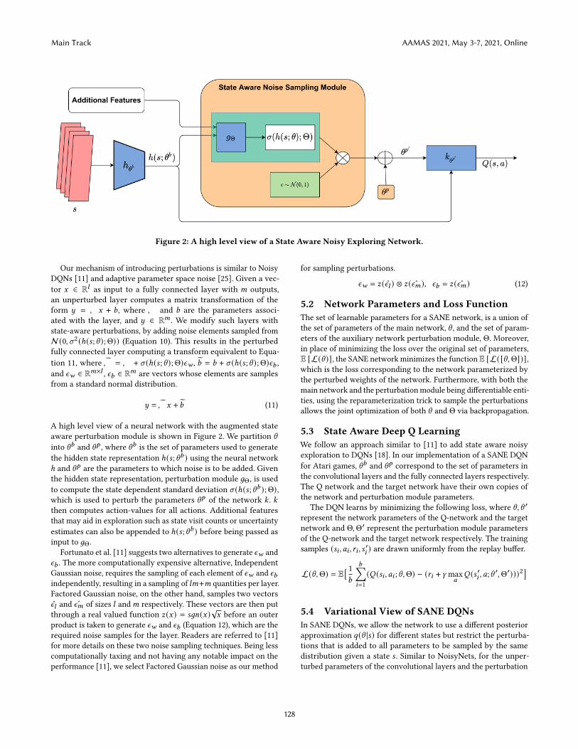
Figure 2: A high level view of a State Aware Noisy Exploring Network.

Our mechanism of introducing perturbations is similar to NoisyDQNs [11] and adaptive parameter space noise [25]. Given a vec-tor 𝑥 ∈ R𝑙 as input to a fully connected layer with 𝑚 outputs,an unperturbed layer computes a matrix transformation of theform 𝑦 = 𝑊𝑥 + 𝑏, where 𝑊 and 𝑏 are the parameters associ-ated with the layer, and 𝑦 ∈ R𝑚 . We modify such layers withstate-aware perturbations, by adding noise elements sampled fromN(0, 𝜎2 (ℎ(𝑠;\ );Θ)) (Equation 10). This results in the perturbedfully connected layer computing a transform equivalent to Equa-tion 11, where𝑊 = 𝑊 + 𝜎 (ℎ(𝑠;\ );Θ)𝜖𝑤 , 𝑏 = 𝑏 + 𝜎 (ℎ(𝑠;\ );Θ)𝜖𝑏 ,and 𝜖𝑤 ∈ R𝑚×𝑙 , 𝜖𝑏 ∈ R𝑚 are vectors whose elements are samplesfrom a standard normal distribution.

𝑦 =𝑊𝑥 + 𝑏 (11)

A high level view of a neural network with the augmented stateaware perturbation module is shown in Figure 2. We partition \into \𝑏 and \𝑝 , where \𝑏 is the set of parameters used to generatethe hidden state representation ℎ(𝑠;\𝑏 ) using the neural networkℎ and \𝑝 are the parameters to which noise is to be added. Giventhe hidden state representation, perturbation module 𝑔Θ, is usedto compute the state dependent standard deviation 𝜎 (ℎ(𝑠;\𝑏 );Θ),which is used to perturb the parameters \𝑝 of the network 𝑘 . 𝑘then computes action-values for all actions. Additional featuresthat may aid in exploration such as state visit counts or uncertaintyestimates can also be appended to ℎ(𝑠;\𝑏 ) before being passed asinput to 𝑔Θ.

Fortunato et al. [11] suggests two alternatives to generate 𝜖𝑤 and𝜖𝑏 . The more computationally expensive alternative, IndependentGaussian noise, requires the sampling of each element of 𝜖𝑤 and 𝜖𝑏independently, resulting in a sampling of 𝑙𝑚+𝑚 quantities per layer.Factored Gaussian noise, on the other hand, samples two vectors𝜖𝑙 and ˆ𝜖𝑚 of sizes 𝑙 and𝑚 respectively. These vectors are then putthrough a real valued function 𝑧 (𝑥) = 𝑠𝑔𝑛(𝑥)

√𝑥 before an outer

product is taken to generate 𝜖𝑤 and 𝜖𝑏 (Equation 12), which are therequired noise samples for the layer. Readers are referred to [11]for more details on these two noise sampling techniques. Being lesscomputationally taxing and not having any notable impact on theperformance [11], we select Factored Gaussian noise as our method

for sampling perturbations.

𝜖𝑤 = 𝑧 (𝜖𝑙 ) ⊗ 𝑧 ( ˆ𝜖𝑚), 𝜖𝑏 = 𝑧 ( ˆ𝜖𝑚) (12)

5.2 Network Parameters and Loss FunctionThe set of learnable parameters for a SANE network, is a union ofthe set of parameters of the main network, \ , and the set of param-eters of the auxiliary network perturbation module, Θ. Moreover,in place of minimizing the loss over the original set of parameters,E [L(\ )], the SANE network minimizes the function E [L([\,Θ])],which is the loss corresponding to the network parameterized bythe perturbed weights of the network. Furthermore, with both themain network and the perturbationmodule being differentiable enti-ties, using the reparameterization trick to sample the perturbationsallows the joint optimization of both \ and Θ via backpropagation.

5.3 State Aware Deep Q LearningWe follow an approach similar to [11] to add state aware noisyexploration to DQNs [18]. In our implementation of a SANE DQNfor Atari games, \𝑏 and \𝑝 correspond to the set of parameters inthe convolutional layers and the fully connected layers respectively.The Q network and the target network have their own copies ofthe network and perturbation module parameters.

The DQN learns by minimizing the following loss, where \, \ ′represent the network parameters of the Q-network and the targetnetwork and Θ,Θ′ represent the perturbation module parametersof the Q-network and the target network respectively. The trainingsamples (𝑠𝑖 , 𝑎𝑖 , 𝑟𝑖 , 𝑠 ′𝑖 ) are drawn uniformly from the replay buffer.

L(\,Θ) = E[ 1𝑏

𝑏∑𝑖=1

(𝑄 (𝑠𝑖 , 𝑎𝑖 ;\,Θ) − (𝑟𝑖 + 𝛾 max𝑎𝑄 (𝑠 ′𝑖 , 𝑎;\

′,Θ′)))2]

5.4 Variational View of SANE DQNsIn SANE DQNs, we allow the network to use a different posteriorapproximation 𝑞(\ |𝑠) for different states but restrict the perturba-tions that is added to all parameters to be sampled by the samedistribution given a state 𝑠 . Similar to NoisyNets, for the unper-turbed parameters of the convolutional layers and the perturbation

Main Track AAMAS 2021, May 3-7, 2021, Online

128

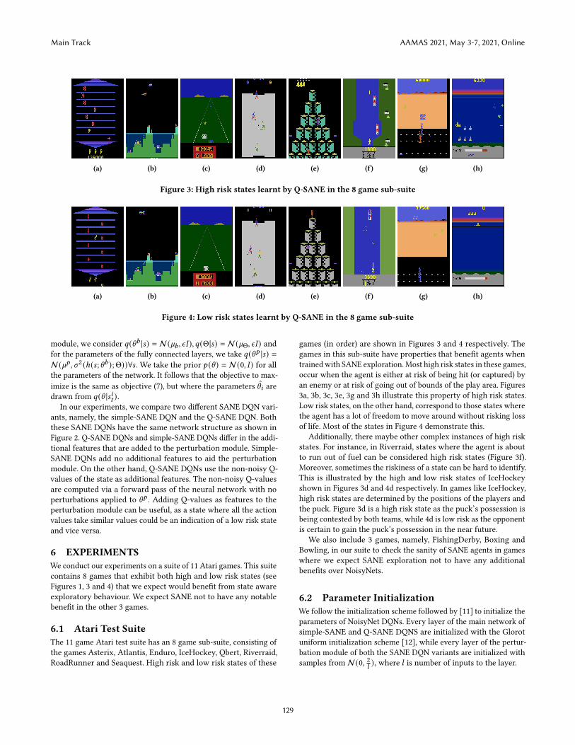
(a) (b) (c) (d) (e) (f) (g) (h)

Figure 3: High risk states learnt by Q-SANE in the 8 game sub-suite

(a) (b) (c) (d) (e) (f) (g) (h)

Figure 4: Low risk states learnt by Q-SANE in the 8 game sub-suite

module, we consider 𝑞(\𝑏 |𝑠) = N(`𝑏 , 𝜖𝐼 ), 𝑞(Θ|𝑠) = N(`Θ, 𝜖𝐼 ) andfor the parameters of the fully connected layers, we take 𝑞(\𝑝 |𝑠) =N(`𝑝 , 𝜎2 (ℎ(𝑠;\𝑏 );Θ))∀𝑠 . We take the prior 𝑝 (\ ) = N(0, 𝐼 ) for allthe parameters of the network. It follows that the objective to max-imize is the same as objective (7), but where the parameters \̂𝑖 aredrawn from 𝑞(\ |𝑠𝑖𝑡 ).

In our experiments, we compare two different SANE DQN vari-ants, namely, the simple-SANE DQN and the Q-SANE DQN. Boththese SANE DQNs have the same network structure as shown inFigure 2. Q-SANE DQNs and simple-SANE DQNs differ in the addi-tional features that are added to the perturbation module. Simple-SANE DQNs add no additional features to aid the perturbationmodule. On the other hand, Q-SANE DQNs use the non-noisy Q-values of the state as additional features. The non-noisy Q-valuesare computed via a forward pass of the neural network with noperturbations applied to \𝑝 . Adding Q-values as features to theperturbation module can be useful, as a state where all the actionvalues take similar values could be an indication of a low risk stateand vice versa.

6 EXPERIMENTSWe conduct our experiments on a suite of 11 Atari games. This suitecontains 8 games that exhibit both high and low risk states (seeFigures 1, 3 and 4) that we expect would benefit from state awareexploratory behaviour. We expect SANE not to have any notablebenefit in the other 3 games.

6.1 Atari Test SuiteThe 11 game Atari test suite has an 8 game sub-suite, consisting ofthe games Asterix, Atlantis, Enduro, IceHockey, Qbert, Riverraid,RoadRunner and Seaquest. High risk and low risk states of these

games (in order) are shown in Figures 3 and 4 respectively. Thegames in this sub-suite have properties that benefit agents whentrainedwith SANE exploration. Most high risk states in these games,occur when the agent is either at risk of being hit (or captured) byan enemy or at risk of going out of bounds of the play area. Figures3a, 3b, 3c, 3e, 3g and 3h illustrate this property of high risk states.Low risk states, on the other hand, correspond to those states wherethe agent has a lot of freedom to move around without risking lossof life. Most of the states in Figure 4 demonstrate this.

Additionally, there maybe other complex instances of high riskstates. For instance, in Riverraid, states where the agent is aboutto run out of fuel can be considered high risk states (Figure 3f).Moreover, sometimes the riskiness of a state can be hard to identify.This is illustrated by the high and low risk states of IceHockeyshown in Figures 3d and 4d respectively. In games like IceHockey,high risk states are determined by the positions of the players andthe puck. Figure 3d is a high risk state as the puck’s possession isbeing contested by both teams, while 4d is low risk as the opponentis certain to gain the puck’s possession in the near future.

We also include 3 games, namely, FishingDerby, Boxing andBowling, in our suite to check the sanity of SANE agents in gameswhere we expect SANE exploration not to have any additionalbenefits over NoisyNets.

6.2 Parameter InitializationWe follow the initialization scheme followed by [11] to initialize theparameters of NoisyNet DQNs. Every layer of the main network ofsimple-SANE and Q-SANE DQNS are initialized with the Glorotuniform initialization scheme [12], while every layer of the pertur-bation module of both the SANE DQN variants are initialized withsamples from N(0, 2

𝑙), where 𝑙 is number of inputs to the layer.

Main Track AAMAS 2021, May 3-7, 2021, Online

129

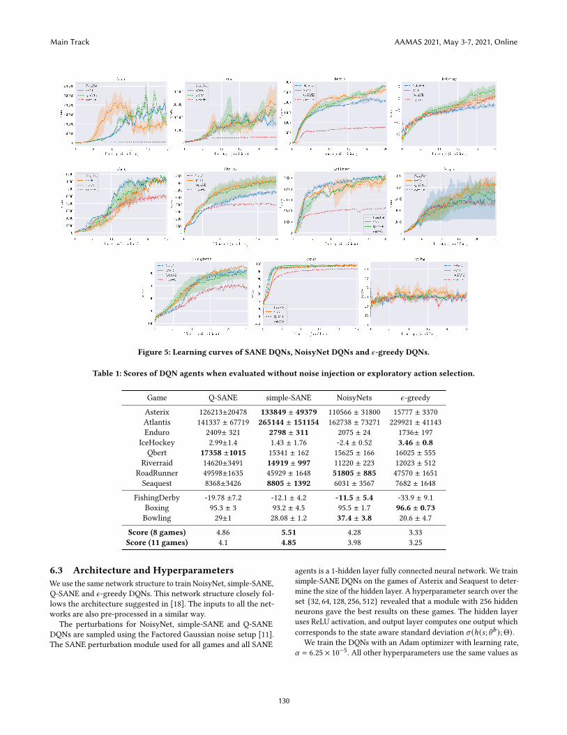
Figure 5: Learning curves of SANE DQNs, NoisyNet DQNs and 𝜖-greedy DQNs.

Table 1: Scores of DQN agents when evaluated without noise injection or exploratory action selection.

Game Q-SANE simple-SANE NoisyNets 𝜖-greedy

Asterix 126213±20478 133849 ± 49379 110566 ± 31800 15777 ± 3370Atlantis 141337 ± 67719 265144 ± 151154 162738 ± 73271 229921 ± 41143Enduro 2409± 321 2798 ± 311 2075 ± 24 1736± 197

IceHockey 2.99±1.4 1.43 ± 1.76 -2.4 ± 0.52 3.46 ± 0.8Qbert 17358 ±1015 15341 ± 162 15625 ± 166 16025 ± 555

Riverraid 14620±3491 14919 ± 997 11220 ± 223 12023 ± 512RoadRunner 49598±1635 45929 ± 1648 51805 ± 885 47570 ± 1651Seaquest 8368±3426 8805 ± 1392 6031 ± 3567 7682 ± 1648

FishingDerby -19.78 ±7.2 -12.1 ± 4.2 -11.5 ± 5.4 -33.9 ± 9.1Boxing 95.3 ± 3 93.2 ± 4.5 95.5 ± 1.7 96.6 ± 0.73Bowling 29±1 28.08 ± 1.2 37.4 ± 3.8 20.6 ± 4.7

Score (8 games) 4.86 5.51 4.28 3.33Score (11 games) 4.1 4.85 3.98 3.25

6.3 Architecture and HyperparametersWe use the same network structure to train NoisyNet, simple-SANE,Q-SANE and 𝜖-greedy DQNs. This network structure closely fol-lows the architecture suggested in [18]. The inputs to all the net-works are also pre-processed in a similar way.

The perturbations for NoisyNet, simple-SANE and Q-SANEDQNs are sampled using the Factored Gaussian noise setup [11].The SANE perturbation module used for all games and all SANE

agents is a 1-hidden layer fully connected neural network. We trainsimple-SANE DQNs on the games of Asterix and Seaquest to deter-mine the size of the hidden layer. A hyperparameter search over theset {32, 64, 128, 256, 512} revealed that a module with 256 hiddenneurons gave the best results on these games. The hidden layeruses ReLU activation, and output layer computes one output whichcorresponds to the state aware standard deviation 𝜎 (ℎ(𝑠;\𝑏 );Θ).

We train the DQNs with an Adam optimizer with learning rate,𝛼 = 6.25 × 10−5. All other hyperparameters use the same values as

Main Track AAMAS 2021, May 3-7, 2021, Online

130

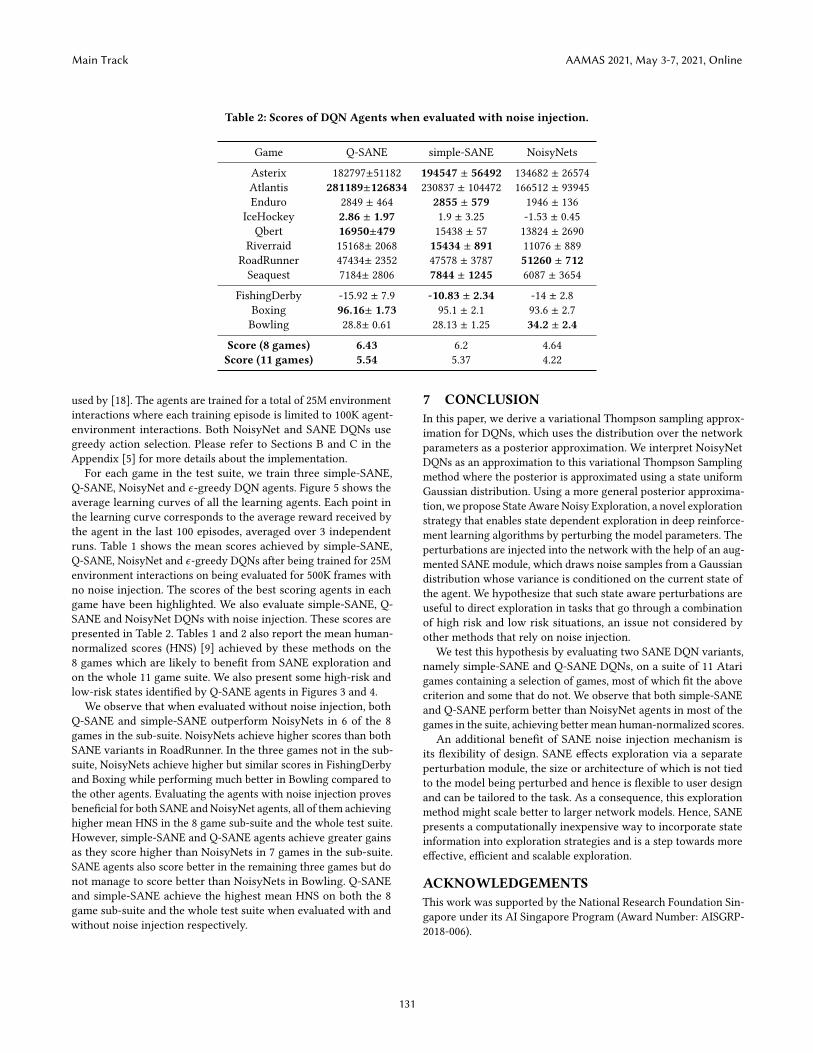
Table 2: Scores of DQN Agents when evaluated with noise injection.

Game Q-SANE simple-SANE NoisyNets

Asterix 182797±51182 194547 ± 56492 134682 ± 26574Atlantis 281189±126834 230837 ± 104472 166512 ± 93945Enduro 2849 ± 464 2855 ± 579 1946 ± 136

IceHockey 2.86 ± 1.97 1.9 ± 3.25 -1.53 ± 0.45Qbert 16950±479 15438 ± 57 13824 ± 2690

Riverraid 15168± 2068 15434 ± 891 11076 ± 889RoadRunner 47434± 2352 47578 ± 3787 51260 ± 712Seaquest 7184± 2806 7844 ± 1245 6087 ± 3654

FishingDerby -15.92 ± 7.9 -10.83 ± 2.34 -14 ± 2.8Boxing 96.16± 1.73 95.1 ± 2.1 93.6 ± 2.7Bowling 28.8± 0.61 28.13 ± 1.25 34.2 ± 2.4

Score (8 games) 6.43 6.2 4.64Score (11 games) 5.54 5.37 4.22

used by [18]. The agents are trained for a total of 25M environmentinteractions where each training episode is limited to 100K agent-environment interactions. Both NoisyNet and SANE DQNs usegreedy action selection. Please refer to Sections B and C in theAppendix [5] for more details about the implementation.

For each game in the test suite, we train three simple-SANE,Q-SANE, NoisyNet and 𝜖-greedy DQN agents. Figure 5 shows theaverage learning curves of all the learning agents. Each point inthe learning curve corresponds to the average reward received bythe agent in the last 100 episodes, averaged over 3 independentruns. Table 1 shows the mean scores achieved by simple-SANE,Q-SANE, NoisyNet and 𝜖-greedy DQNs after being trained for 25Menvironment interactions on being evaluated for 500K frames withno noise injection. The scores of the best scoring agents in eachgame have been highlighted. We also evaluate simple-SANE, Q-SANE and NoisyNet DQNs with noise injection. These scores arepresented in Table 2. Tables 1 and 2 also report the mean human-normalized scores (HNS) [9] achieved by these methods on the8 games which are likely to benefit from SANE exploration andon the whole 11 game suite. We also present some high-risk andlow-risk states identified by Q-SANE agents in Figures 3 and 4.

We observe that when evaluated without noise injection, bothQ-SANE and simple-SANE outperform NoisyNets in 6 of the 8games in the sub-suite. NoisyNets achieve higher scores than bothSANE variants in RoadRunner. In the three games not in the sub-suite, NoisyNets achieve higher but similar scores in FishingDerbyand Boxing while performing much better in Bowling compared tothe other agents. Evaluating the agents with noise injection provesbeneficial for both SANE and NoisyNet agents, all of them achievinghigher mean HNS in the 8 game sub-suite and the whole test suite.However, simple-SANE and Q-SANE agents achieve greater gainsas they score higher than NoisyNets in 7 games in the sub-suite.SANE agents also score better in the remaining three games but donot manage to score better than NoisyNets in Bowling. Q-SANEand simple-SANE achieve the highest mean HNS on both the 8game sub-suite and the whole test suite when evaluated with andwithout noise injection respectively.

7 CONCLUSIONIn this paper, we derive a variational Thompson sampling approx-imation for DQNs, which uses the distribution over the networkparameters as a posterior approximation. We interpret NoisyNetDQNs as an approximation to this variational Thompson Samplingmethod where the posterior is approximated using a state uniformGaussian distribution. Using a more general posterior approxima-tion, we propose State Aware Noisy Exploration, a novel explorationstrategy that enables state dependent exploration in deep reinforce-ment learning algorithms by perturbing the model parameters. Theperturbations are injected into the network with the help of an aug-mented SANE module, which draws noise samples from a Gaussiandistribution whose variance is conditioned on the current state ofthe agent. We hypothesize that such state aware perturbations areuseful to direct exploration in tasks that go through a combinationof high risk and low risk situations, an issue not considered byother methods that rely on noise injection.

We test this hypothesis by evaluating two SANE DQN variants,namely simple-SANE and Q-SANE DQNs, on a suite of 11 Atarigames containing a selection of games, most of which fit the abovecriterion and some that do not. We observe that both simple-SANEand Q-SANE perform better than NoisyNet agents in most of thegames in the suite, achieving better mean human-normalized scores.

An additional benefit of SANE noise injection mechanism isits flexibility of design. SANE effects exploration via a separateperturbation module, the size or architecture of which is not tiedto the model being perturbed and hence is flexible to user designand can be tailored to the task. As a consequence, this explorationmethod might scale better to larger network models. Hence, SANEpresents a computationally inexpensive way to incorporate stateinformation into exploration strategies and is a step towards moreeffective, efficient and scalable exploration.

ACKNOWLEDGEMENTSThis work was supported by the National Research Foundation Sin-gapore under its AI Singapore Program (Award Number: AISGRP-2018-006).

Main Track AAMAS 2021, May 3-7, 2021, Online

131

REFERENCES[1] Joshua Achiam and Shankar Sastry. 2017. Surprise-Based Intrinsic Motivation

for Deep Reinforcement Learning. arXiv preprint arXiv:1703.01732 (2017).[2] Shipra Agrawal and Navin Goyal. 2012. Analysis of Thompson Sampling for the

Multi-Armed Bandit Problem. In Conference on Learning Theory. 39–1.[3] Shipra Agrawal and Navin Goyal. 2013. Further Optimal Regret Bounds for

Thompson Sampling. In Artificial Intelligence and Statistics. 99–107.[4] Shipra Agrawal and Randy Jia. 2017. Optimistic Posterior Sampling for Reinforce-

ment Learning: Worst-Case Regret Bounds. In Advances in Neural InformationProcessing Systems. 1184–1194.

[5] Siddharth Aravindan and Wee Sun Lee. 2021. State-Aware Variational ThompsonSampling for Deep Q-Networks. ArXiv e-prints (2021).

[6] Peter Auer and Ronald Ortner. 2007. Logarithmic Online Regret Bounds for Undis-counted Reinforcement Learning. In Advances in Neural Information ProcessingSystems. 49–56.

[7] Kamyar Azizzadenesheli, Emma Brunskill, and Animashree Anandkumar. 2018.Efficient Exploration through Bayesian Deep Q-Networks. In 2018 InformationTheory and Applications Workshop (ITA). IEEE, 1–9.

[8] Marc Bellemare, Sriram Srinivasan, Georg Ostrovski, Tom Schaul, David Sax-ton, and Remi Munos. 2016. Unifying Count-Based Exploration and IntrinsicMotivation. In Advances in Neural Information Processing Systems. 1471–1479.

[9] Marc Brittain, Joshua R. Bertram, Xuxi Yang, and Peng Wei. 2019. PrioritizedSequence Experience Replay. CoRR abs/1905.12726 (2019). arXiv:1905.12726http://arxiv.org/abs/1905.12726

[10] Carlos Florensa, Yan Duan, and Pieter Abbeel. 2017. Stochastic Neural Networksfor Hierarchical Reinforcement Learning. In International Conference on LearningRepresentations. https://openreview.net/forum?id=B1oK8aoxe

[11] Meire Fortunato, Mohammad Gheshlaghi Azar, Bilal Piot, Jacob Menick, MatteoHessel, Ian Osband, Alex Graves, Volodymyr Mnih, Remi Munos, Demis Hassabis,Olivier Pietquin, Charles Blundell, and Shane Legg. 2018. Noisy Networks ForExploration. In International Conference on Learning Representations. https://openreview.net/forum?id=rywHCPkAW

[12] Xavier Glorot and Yoshua Bengio. 2010. Understanding the Difficulty of TrainingDeep Feedforward Neural Networks. In Proceedings of The Thirteenth InternationalConference on Artificial Intelligence and Statistics. 249–256.

[13] Shixiang Gu, Ethan Holly, Timothy Lillicrap, and Sergey Levine. 2017. DeepReinforcement Learning for Robotic Manipulation with Asynchronous Off-PolicyUpdates. In 2017 IEEE International Conference on Robotics and Automation (ICRA).IEEE, 3389–3396.

[14] Thomas Jaksch, Ronald Ortner, and Peter Auer. 2010. Near-Optimal RegretBounds for Reinforcement Learning. Journal of Machine Learning Research 11,Apr (2010), 1563–1600.

[15] Emilie Kaufmann, Nathaniel Korda, and Rémi Munos. 2012. Thompson Sampling:An Asymptotically Optimal Finite-Time Analysis. In International Conference onAlgorithmic Learning Theory. Springer, 199–213.

[16] Elias Khalil, Hanjun Dai, Yuyu Zhang, Bistra Dilkina, and Le Song. 2017. LearningCombinatorial Optimization Algorithms over Graphs. In Advances in NeuralInformation Processing Systems. 6348–6358.

[17] Xiaodan Liang, Lisa Lee, and Eric P Xing. 2017. Deep Variation-StructuredReinforcement Learning for Visual Relationship and Attribute Detection. In

Proceedings of the IEEE Conference on Computer Vision and Pattern Recognition.848–857.

[18] Volodymyr Mnih, Koray Kavukcuoglu, David Silver, Andrei A Rusu, Joel Ve-ness, Marc G Bellemare, Alex Graves, Martin Riedmiller, Andreas K Fidjeland,Georg Ostrovski, et al. 2015. Human-Level Control through Deep ReinforcementLearning. Nature 518, 7540 (2015), 529.

[19] IanOsband, JohnAslanides, andAlbin Cassirer. 2018. Randomized Prior Functionsfor Deep Reinforcement Learning. In Advances in Neural Information ProcessingSystems. 8617–8629.

[20] Ian Osband, Charles Blundell, Alexander Pritzel, and Benjamin Van Roy. 2016.Deep Exploration via Bootstrapped DQN. In Advances in Neural InformationProcessing Systems. 4026–4034.

[21] Ian Osband and Benjamin Van Roy. 2015. Bootstrapped Thompson Sampling andDeep Exploration. arXiv preprint arXiv:1507.00300 (2015).

[22] Ian Osband and Benjamin Van Roy. 2017. Why is Posterior Sampling Better thanOptimism for Reinforcement Learning?. In International Conference on MachineLearning. 2701–2710.

[23] Ian Osband, Benjamin Van Roy, and Zheng Wen. 2016. Generalization and Explo-ration via Randomized Value Functions. In Proceedings of the 33rd InternationalConference on Machine Learning-Volume 48. JMLR. org, 2377–2386.

[24] Georg Ostrovski, Marc G Bellemare, Aäron van den Oord, and Rémi Munos. 2017.Count-Based Exploration with Neural Density Models. In Proceedings of the 34thInternational Conference on Machine Learning-Volume 70. JMLR. org, 2721–2730.

[25] Matthias Plappert, Rein Houthooft, Prafulla Dhariwal, Szymon Sidor, Richard Y.Chen, Xi Chen, Tamim Asfour, Pieter Abbeel, and Marcin Andrychowicz. 2018.Parameter Space Noise for Exploration. In International Conference on LearningRepresentations. https://openreview.net/forum?id=ByBAl2eAZ

[26] Thomas Rückstieß, Frank Sehnke, Tom Schaul, DaanWierstra, Yi Sun, and JürgenSchmidhuber. 2010. Exploring Parameter Space in Reinforcement Learning.Paladyn 1, 1 (2010), 14–24.

[27] Tim Salimans, Jonathan Ho, Xi Chen, Szymon Sidor, and Ilya Sutskever. 2017.Evolution Strategies as a Scalable Alternative to Reinforcement Learning. arXivpreprint arXiv:1703.03864 (2017).

[28] Bradly C Stadie, Sergey Levine, and Pieter Abbeel. 2015. Incentivizing Explo-ration in Reinforcement Learning with Deep Predictive Models. arXiv preprintarXiv:1507.00814 (2015).

[29] Malcolm Strens. 2000. A Bayesian Framework for Reinforcement Learning. InInternational Conference on Machine Learning, Vol. 2000. 943–950.

[30] Richard S Sutton and Andrew G Barto. 2018. Reinforcement learning: An Intro-duction. MIT press.

[31] Adrien Ali Taiga, William Fedus, Marlos C. Machado, Aaron Courville, andMarc G. Bellemare. 2020. On Bonus Based Exploration Methods In The ArcadeLearning Environment. In International Conference on Learning Representations.https://openreview.net/forum?id=BJewlyStDr

[32] William R Thompson. 1933. On the Likelihood that One Unknown ProbabilityExceeds Another in View of the Evidence of Two Samples. Biometrika 25, 3/4(1933), 285–294.

[33] Sirui Xie, Junning Huang, Lanxin Lei, Chunxiao Liu, Zheng Ma, Wei Zhang, andLiang Lin. 2019. NADPEx: An On-Policy Temporally Consistent ExplorationMethod for Deep Reinforcement Learning. In International Conference on LearningRepresentations. https://openreview.net/forum?id=rkxciiC9tm

Main Track AAMAS 2021, May 3-7, 2021, Online

132