arX

iv:1

001.

3935

v1 [

mat

h.O

C]

22

Jan

2010

Proceedings of the International Workshop on Statistical-Mechanical Informatics

March 7–10, 2010, Kyoto, Japan

Cavity approach to the first eigenvalue problem in a

family of symmetric random sparse matrices

Yoshiyuki Kabashima†1, Hisanao Takahashi†2 and Osamu Watanabe‡3

†Department of Computational Intelligence and Systems Science, Tokyo Institute ofTechnology, Yokohama 226-8502, Japan‡Department of Mathematical and Computing Science, Tokyo Institute of Technology, Tokyo152-8552, Japan

E-mail: 1kaba@dis.titech.ac.jp,

2takahashi@sp.dis.titech.ac.jp,

3watanabe@is.titech.ac.jp

Abstract. A methodology to analyze the properties of the first (largest) eigenvalue and itseigenvector is developed for large symmetric random sparse matrices utilizing the cavity methodof statistical mechanics. Under a tree approximation, which is plausible for infinitely largesystems, in conjunction with the introduction of a Lagrange multiplier for constraining thelength of the eigenvector, the eigenvalue problem is reduced to a bunch of optimization problemsof a quadratic function of a single variable, and the coefficients of the first and the second orderterms of the functions act as cavity fields that are handled in cavity analysis. We show thatthe first eigenvalue is determined in such a way that the distribution of the cavity fields hasa finite value for the second order moment with respect to the cavity fields of the first ordercoefficient. The validity and utility of the developed methodology are examined by applyingit to two analytically solvable and one simple but non-trivial examples in conjunction withnumerical justification.

1. Introduction

The first (largest) eigenvalue and its eigenvector (first eigenvector) play key roles in manyproblems in information science. In multivariate data analysis, the first eigenvector of thevariance-covariance matrix represents the most significant component that underlies a set of dataunder the assumption that the data are generated from a multivariate Gaussian distribution,and the first eigenvalue indicates its relevance [1]. The well-known Google PageRankTM ranksWorld Wide Web pages based on the first eigenvector of a transition matrix over a huge networkof pages [2]. The first eigenvectors of certain matrices expressing a given graph can also beutilized as a practical solution to combinatorial problems such as graph three coloring- [3] andgraph bisection problems [4].

The first eigenvalue problem is of significance in physics as well. The assessment of theground state is generally formulated as a first eigenvalue problem in quantum mechanics [5]. Itis generally difficult to accurately assess the correlations in spin systems in statistical mechanics.However, when the temperature is sufficiently high, spin correlations can be evaluated byreplacing spin variables with so-called spherical spins in a class of systems [6], which is practicallyreduced to the eigenvalue analysis of the interaction matrix. In particular, that for the firsteigenvalue is of great relevance because it directly leads to the assessment of the critical

temperature/mode for the emergence of spontaneous magnetization [7].Many properties have thus far been clarified for the first eigenvalue problem for the ensembles

of large dense matrices. For N ×N symmetric matrices S whose entries are independently andidentically distributed (i.i.d.) random variables of a zero mean and a variance of N−1, the firsteigenvalue asymptotically converges to 2 and the first eigenvector has no preferential directions inthe N -dimensional space as N tends toward infinity [8]. However, when a projection operator ofa certain direction, d, is added to S with an amplitude, B, the asymptotic eigenvalue is switchedto B + 1/B for B > 1 having a first eigenvector of a non-zero overlap with d. Similar resultsare also obtained for the correlation matrix, P−1

XTX, of P × N matrices X whose entries

i.i.d. random variables of a zero mean and variance N−1, where T denotes the operation of thematrix transpose; the first eigenvalue is offered as (1+α−1/2)2 in the limit of N,P → ∞ keepingα = P/N finite providing no preferential directions of the first eigenvector [9], and the analysiscan also be generalized to cases in which the projection operators of several directions witharbitrary strengths are added [10]. However, as far as we know, relatively little knowledge hasbeen gained on ensembles of sparse matrices in which the density of non-zero entries vanishesas the size of the matrices tends to infinity although details on eigenvalue distributions haverecently been unraveled for several cases [11, 12, 13, 14, 15, 16].

Based on such an understanding, we will herein examine the first eigenvalue and thedistribution of components of the first eigenvector for a family of large symmetric random sparsematrices. To achieve this purpose, we employ the cavity method of statistical mechanics [17].A major advantage of this scheme is its capability for deriving equations for macroscopicallycharacterizing objective systems without having to resort to complicated computation that isgenerally demanded in an alternative approach termed the replica method [18], on the basis ofa tree approximation, which is intuitively plausible for large sparse matrices

This paper is organized as follows. The next section introduces the model that will beexplored. In section 3, we develop a scheme for examining the eigenvalue problem in a largesystem limit based on the cavity method. The scheme is applied to two analytically solvableand one simple but nontrivial examples in section 4. The final section is devoted to a summary.

2. Model definition

We consider ensembles of N×N real symmetric sparse matrices J = (Jij) that are characterizedby a distribution, p(k), of degree k(= 0, 1, 2, . . .), which denotes the number of non-zero entriesfor a column/row in the limit of N → ∞. For simplicity, we assume that the diagonal elementsof the matrices are always constrained to zero. For aspects other than degrees, we assume thatthe matrices are randomly constructed. Let us denote di as the degree of index i(= 1, 2, . . . , N).For k = 0, 1, 2, . . ., we set di = k for Np(k) indices of i = 1, 2, . . . , N . A practical scheme forgenerating a random configuration of non-zero entries characterized in the above is basically asfollows [19]:

(S) Make a set of indices U to which each index i attends di times. Accordingly, we iterate thefollowing (A)–(C).

(A) Choose a pair of two different elements from U randomly.

(B) Let us denote the values of the two elements as i and j. If i 6= j and the pair of i and jhas not been chosen up to the moment, make a link between i and j, and remove the twoelements from U . Otherwise, we return them back to U .

(C) If U becomes empty, finish the iteration. Otherwise, if there is no possibility that any morelinks can be made by (A) and (B), return to (S).

Links generated by the above procedure stand for pairs of indices i and j to which thenon-zero entries of Jij are assigned. There may be other algorithms for randomly generating

a configuration of the non-zero entries. However, we expect that the properties, which we willinvestigate after this, do not depend on the details of the generation schemes.

When the support of p(k) is not bounded from the above and values of the entries are keptfinite, the first eigenvalue generally diverges as N → ∞ [11, 12, 13, 14, 15, 16]. To avoidthis possibility, we assume that p(k) = 0 for k, which is larger than a certain value, kmax,unless infinitesimal entries are assumed. We also assume that the non-zero elements of Jij aredetermined as statistically independent samples following an identical distribution, pJ(Jij). Incases where pJ(Jij) is provided by a simple binary distribution,

pJ(Jij |∆, J) =1 + ∆

2δ(Jij − J) +

1−∆

2δ(Jij + J) (1)

(1 ≥ ∆ ≥ 0, J > 0), where δ(x) denotes Dirac’s delta function, these guarantee that the firsteigenvalue Λ is bounded from the above by kmaxJ .

In matrix ensembles of Erdos-Renyi type [20], which have been widely studied in networkscience, a non-zero value of Jij is assigned to each pair of indices i > j with a certain probability,c/N , where c > 0 is O(1). This eventually leads to a Poissonian degree distribution asp(k) = e−cck/k!, whose support is not bounded from the above. Therefore, the following analysisdoes not cover such ensembles as long as the matrix entries are O(1).

3. Cavity approach to first eigenvalue problem

3.1. Message passing in fixed graph

Formulating the first eigenvalue problem as a constrained quadratic optimization problem

minv

{

−vTJv}

subject to |v|2 = N (2)

is the basis of our analysis, where minX{· · ·} denotes minimization with respect to X. Thesolution to this problem v

∗ = (v∗i ) represents the first eigenvector that is normalized to√N and

the first eigenvalue Λ is assessed as Λ = (v∗)TJv∗/N . The introduction of a Lagrange multiplierλ converts (2) to a saddle point problem with respect to an objective function,

L(v, λ) = −vTJv + λ(|v|2 −N)

= λ∑

i=1

v2i − 2∑

i>j

Jijvivj −Nλ. (3)

Minimizing this function with respect to v and determining λ so as to satisfy the stationarycondition, |v|2 = N , indicate that the solution is provided by the first eigenvalue, λ = Λ, andthe first eigenvector, v = v

∗.The key idea underlying our approach is to approximate the minimization problem of (3)

with respect to v for fixed λ by a bunch of those for effective quadratic functions of a singlevariable

Li(vi|Ai,Hi) = Aiv2i − 2Hivi (4)

(i = 1, 2, . . . , N), where the coefficients of the second and first order terms, Ai and Hi, aredetermined in a certain self-consistent manner. In the cavity method, these coefficients areevaluated by a message-passing algorithm that yields the exact solution when the connectivityof Jij is pictorially represented by a cycle free graph (tree).

To explain this, let us focus on an arbitrary index, i, assuming that matrix connectivity isspecified by a tree. We use a notation, ∂i, to represent the set of indices j that are connected

directly to i with non-zero entries of Jij . We also introduce auxiliary variables Aj→i and Hj→i

to represent the second and first order coefficients of j ∈ ∂i in the i-cavity system, which isdefined by removing index i from the original system. In physics, such variables are occasionallytermed cavity fields.

A general and distinctive feature of trees is that all indices j ∈ ∂i are completely disjointedfrom one another by removing the index, i. Let us assume that we add i into the i-cavity systemretaining one link Jli for an index, l ∈ ∂i, removed. This creates a problem with minimizing afunction with respect to the vi and vj of j ∈ ∂i\l, where S\l indicates the removal of l from aset, S, as

Li,∂i\l(vi, {vj∈∂i\l}) = λv2i − 2vi∑

j∈∂i\l

Jijvj +∑

j∈∂i\l

(

Aj→iv2j − 2Hj→ivj

)

. (5)

Since i is connected to l only with Jli in the original tree, minimizing this function with respectto the vj of ∀j ∈ ∂i\l fixing vi yields cavity fields concerning i in the l-cavity system as

Ai→l = λ−∑

j∈∂i\l

J2ij

Aj→i, (6)

Hi→l =∑

j∈∂i\l

JijHj→i

Aj→i. (7)

Given an initial condition, these equations are capable of assessing sets of the cavity fields, Aj→i

and Hj→i, which are defined for all directed pairs of the connected indices, moving entirely overthe graph. J2

ij/Aj→i and JijHj→i/Aj→i in (6) and (7) represent the influences of j to i conveyedthrough connection Jij and are sometimes referred to as cavity biases. After the cavity fieldsare determined, Ai and Hi in (4) are assessed by summing up the cavity biases from ∀j ∈ ∂ias Ai = λ −

∑

j∈∂i J2ij/Aj→i and Hi =

∑

j∈∂i JijHj→i/Aj→i. This yields v∗i = Hi/Ai. Finally,

adjusting λ so that the normalization constraint, |v∗|2 =∑N

i=1(v∗i )

2 =∑N

i=1(Hi/Ai)

2 = N , issatisfied provides Λ.

The above procedure can be regarded as a variant of the belief propagation developed inresearch on probabilistic inference [21] and is guaranteed to offer the exact result when thegraph is free from cycles. When the graph contains cycles, the algorithm in (6) and (7) can stillbe performed; unfortunately, the result obtained is just an approximation. However, for ourcurrent purpose, we can generally utilize a much simpler and exact method that just repeatsmatrix multiplication as v

t+1 = (aIN + J)vt, which provides Λ = limt→∞ |vt+1|/|vt| − aand v

∗ =√N limt→∞ v

t/|vt|, where a is a sufficiently large positive number and IN denotesthe N × N identity matrix. Therefore, our approach may seem less competitive in practice.However, the cavity approach is still useful for examining the properties of the eigenvalue problemintroducing a macroscopic description as is explained below.

3.2. Description by distribution of cavity fields

Let us examine the behavior of the algorithm in (6) and (7). To do this, we need to pay attentionto the property of randomly constructed sparse matrices, which implies that the lengths ofcycles in the connectivity graph of a matrix typically grow as O(lnN) as N → ∞ [22]. Thisnaturally motivates us to ignore the effects of self-interactions in the updates of (6) and (7).We also introduce a macroscopic characterization of the cavity fields utilizing the distribution,q(A,H) = (

∑Ni=1

di)−1∑N

i=1

∑

j∈∂i δ(A − Aj→i)δ(H −Hj→i). When a link in the connectivitygraph is chosen randomly, the probability that the index of one terminal has a degree, k, is

provided as

r(k) =kp(k)

∑kmax

k=0kp(k)

. (8)

This and dealing with (6) and (7) as the elemental process for updating the cavity fielddistribution lead to an equation that determines q(A,H) in a self-consistent manner as

q(A,H)=

kmax∑

k=1

r(k)

∫ k−1∏

j=1

dAjdHjq(Aj ,Hj)

⟨

δ

A− λ+

k−1∑

j=1

J 2j

Aj

δ

H −k−1∑

j=1

JjHj

Aj

⟩

J

, (9)

where 〈· · ·〉J represents the operation of taking averages with respect to all relevant Jj’s

following pJ(Jj). After q(A,H) is determined with this equation, the distribution of the auxiliary

variables in the original system, Q(A,H) = N−1∑N

i=1δ(A−Ai)δ(H −Hi), is assessed as

Q(A,H)=

kmax∑

k=0

p(k)

∫ k∏

j=1

dAjdHjq(Aj ,Hj)

⟨

δ

A− λ+k∑

j=1

J 2j

Aj

δ

H −k∑

j=1

JjHj

Aj

⟩

J

. (10)

This make it possible to evaluate the quadratic norm per element of v∗ as T = N−1|v∗|2 =∫

dAdHQ(A,H)(H/A)2 . Moreover, the distribution of elements of the first eigenvector, v∗, can

be assessed as P (v) = N−1∑N

i=1δ(v − v∗) =

∫

dAdHQ(A,H)δ(v −H/A).The argument provided in the preceding subsection implies that λ should be adjusted so that

T accords with unity. However, here we adopt an alternative approach to determining Λ. Letus assume a situation where (9) is solved by a method of successive iteration, which leads to anexact result when the graph is free from cycles. Equation (9) guarantees that for large λ, A isdistributed over large values in q(A,H). This means that for sufficiently large λ, the absolutevalues of H are mostly reduced by each iteration and, therefore, the marginal distribution,q(H) =

∫

dAq(A,H), converges to δ(H) implying T → 0 as the number of iterations tends toinfinity. However, as λ is decreased from sufficiently large values, A can take smaller values in thedistribution and larger values of |H| could appear with considerable frequency in each iteration.This indicates that the frequencies with which |H| is reduced and enlarged are balanced at acertain value of λ, for which non-trivial distribution q(H) 6= δ(H) becomes invariant under thecavity iteration of (9) and T is kept as a finite constant. If λ is lowered further, the frequencyof enlargements will overcome that of reductions, which will eventually make T tend to infinity.These imply that one can characterize the first eigenvalue, Λ, as the value of λ for which non-trivial distribution q(H) 6= δ(H) emerges by solving (9). The resulting cavity field distribution,q(A,H), offers the distribution of the first eigenvector elements, P (v), of any finite value of T byapplying appropriate rescaling with respect to H. This is also reasonable because eigenvalues aregenerally irrelevant to the values of the normalization constraint with respect to eigenvectors.

The validity and utility of this characterization of the eigenvalue problem are examined byapplying it to three examples in the next section.

4. Application to three examples

4.1. Single degree model

In the first example, we consider cases where all indices have a certain identical degree, K,which is characterized by p(k) = δk,K , where δi,j denotes Kroeneker’s delta, and the non-zeroentries are i.i.d. following the binary distribution of (1). In such cases, the marginal distribution,q(A) =

∫

dHq(A,H), is provided in the form of q(A) = δ(A−A∗) since J 2 = J2 always holds for

0 0.2 0.4 0.6 0.8 10

0.2

0.4

0.6

0.8

1

0 0.2 0.4 0.6 0.8 13.4

3.6

3.8

4

−8 −4 0 4 80

1

2

3

Δ Δ

Λ M

N M

1/6

N ( )/Δ−Δ1/3

c

(a) (b)

Δc

Figure 1. (a): First eigenvalue Λ versus ∆ for single degree model of K = 4 and J = 1. Thefull curve represents the theoretical prediction of (17) while the markers denote the averagesof 2000 experimental results for N = 256 (red), 512 (green) and 1024 (blue) systems. (b):

M = |N−1∑N

i=1v∗i | versus ∆ for the same experiments as (a). Red, green, and blue markers

correspond to N = 256, 512, and 1024 as well. The inset has scaling plots obtained by conversionof M → N1/6M and ∆ → N1/3(∆ − ∆c)/∆c. In both (a) and (b), the vertical straight lines(magenta) stand for ∆c = 1/

√3 = 0.577 . . ..

∀J that are sampled from (1). Equation (9) indicates that A∗ satisfies A∗ = λ− (K − 1)J2/A∗.This yields

A∗ =λ+

√

λ2 − 4(K − 1)J2

2≡ A∗(λ; (K − 1)J2), (11)

which along with (9) offer the equation for determining the marginal distribution, q(H), in aself-consistent manner as

q(H) =

∫ K−1∏

j=1

dHjq(Hj)

⟨

δ

H −K−1∑

j=1

JjHj

A∗(λ; (K − 1)J2)

⟩

J

. (12)

Tuning λ so that a non-trivial distribution, q(H) 6= δ(H), satisfies this equation yields the firsteigenvalue, Λ. Paying attention to the first and the second order moments, m1 =

∫

dHq(H)Hand m2 =

∫

dHq(H)H2, is sufficient for this purpose. This provides a generalized eigenvalueproblem described by a couple of equations

m1 =∆(K − 1)J

A∗(λ; (K − 1)J2)m1, (13)

m2 =(K − 1)J2

(A∗(λ; (K − 1)J2))2(m2 −m2

1) +

(

∆(K − 1)J

A∗(λ; (K − 1)J2)m1

)2

, (14)

which requires the existence of a solution to (m1,m2) 6= (0, 0). There are two possibilities thatwill satisfy this requirement. The first is characterized by |m1| > 0, which in conjunction with(13) offers

1 =∆(K − 1)J

A∗(λ; (K − 1)J2). (15)

−1.5 −1 −0.5 0 0.5 1 1.5 20

0.5

1

1.5

2

v

P(v

)

−6 −4 −2 0 2 4 60

0.1

0.2

0.3

0.4

v

P(v

)(a) (b)

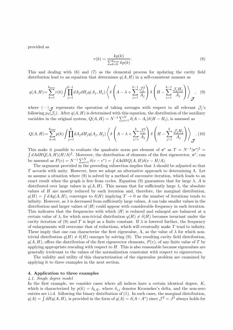
Figure 2. P (v) for (a): ∆ = 0.5 and (b): ∆ = 0.9 of single degree model of K = 4. Forboth plots, the bars represent histograms obtained from 100 experiments of N = 1024 while thecurves stand for theoretical predictions obtained from (12) and (10) by means of a Monte Carlomethod of 106 populations. In handling the experimental data of (b), we employed conversion

v∗ → −v

∗ for data of∑N

i=1v∗i < 0 in order to break the mirror symmetry between v

∗ and −v∗,

which is intrinsic in the eigenvalue problem.

The second is the case of m1 = 0 and m2 > 0, which along with (14) provide

1 =(K − 1)J2

(A∗(λ; (K − 1)J2))2. (16)

Solving (15) and (16) with respect to λ, we finally obtain an expression of the first eigenvalue,

Λ =

{

((K − 1)∆ + 1/∆) J, ∆ > ∆c,2√K − 1J, ∆ < ∆c,

(17)

where ∆c = 1/√K − 1. ∆ > ∆c and ∆ < ∆c correspond to the cases of |m1| > 0 and m1 = 0.

To justify the prediction of (17), we carried out numerical experiments for the systems ofK = 4 and J = 1, whose results are in figures 1 (a) and (b). Figure 1 (a) has the plotsof Λ versus ∆, which are in excellent agreement with (17) for relatively large ∆. However,there are non-negligible finite-size corrections for relatively small ∆, which makes it difficultto accurately detect the critical value, ∆c. To overcome this difficulty, we turn to the profiles

of M =∣

∣

∣N−1

∑Ni=1

v∗i

∣

∣

∣, which are shown in figure 1 (b). The raw experimental data of M

vary smoothly with ∆ and do not exhibit any singularity at ∆ = ∆c either. Nevertheless,the data rescaled as M → N1/6M and ∆ → N1/3(∆ − ∆c)/∆c support a scaling hypothesis,M = N−1/6F (N1/3(∆ − ∆c)/∆c) (inset), which validates the transition at ∆c assuming thatF (x) behaves as O(x1/2) for x → +∞ and vanishes for x → −∞. A similar scaling hypothesishas been assumed in the examination of principal component analysis before [10].

Besides the eigenvalue, one can also assess the distributions, P (v), of elements of the firsteigenvector, v∗, by numerically solving q(H) with Monte Carlo (population dynamics) methods.The prediction with our approach is also in excellent agreement with the experimental results forboth cases of ∆ < ∆c (figure 2 (a)) and ∆ > ∆c (figure 2 (b)) when |∆−∆c|/|∆c| is sufficientlylarge.

4.2. Limit of large degrees and infinitesimal entries

The second example is offered by assuming that the average and the variance of p(k) are providedas k and O(k), respectively, and those of pJ(Jij) are given as µJ/k and J2/k for sufficiently largek while µ > 0 and J > 0 are certain finite constants. The assumption on the degree distribution,p(k), covers the cases described by truncated Poissonian distributions of large mean values inwhich indices whose degrees are sufficiently larger than the means are eliminated from thebasic graphs of Erdos-Renyi type [4]. Being combined with the assumption on pJ(Jji), this,in conjunction with the law of large numbers, guarantees that the marginal distribution of Ais provided as q(A) = δ(A − A∗(λ;J2)), where the functional form of A∗(λ;J2) is identicalto that of (11). Inserting this into (12) and the resulting equations with respect to the firstand the second order moments offer conditions of 1 = µJ/A∗(λ;J2) and 1 = J2/(A∗(λ;J2))2,respectively, which are counterparts of (15) and (16). This provides the first eigenvalue as

Λ =

{

(µ + 1/µ)J, µ > 1,2J, µ < 1.

(18)

µ > 1 and µ < 1 correspond to situations of |m1| > 0 and m1 = 0.In the current case, the central limit theorem guarantees that q(H) converges to a distribution

of the Gaussian type. Consequently, this also makes it possible to analytically express thedistribution, P (v), of the elements of the first eigenvector in a Gaussian form. Under theconstraint of T = 1, this yields

P (v) =

{

(2π(1− (M(µ))2)−1/2 exp(

−(v −M(µ))2/(2(1 − (M(µ))2)))

, µ > 1,

(2π)−1/2 exp(

−v2/2)

, µ < 1,(19)

where M(µ) = ±√

1− 1/µ2.

4.3. Mixture of multiple degrees

The strategy we employed for analyzing the preceding two examples is summarized as follows.We first evaluate the marginal distribution, q(A) =

∫

dHq(A,H), of the second order cavityfields in the form of a single delta distribution, q(A) = δ(A − A∗). This enables us to dealwith A as a constant, A∗, in assessing the marginal distribution, q(H) =

∫

dAq(A,H), of thefirst order cavity fields. Consequently, the original eigenvalue problem is reformulated as ageneralized eigenvalue problem with respect to q(H). This imposes certain conditions on thesecond order cavity field, A∗, which is a function of λ. The first eigenvalue is evaluated bysolving the conditions with respect to λ.

Unfortunately, such clear decoupling of the first and the second order cavity fields cannotgenerally be exploited in handling the eigenvalue problem precisely. Even when p(k) takes finitevalues for multiple k, the marginal distribution, q(A), constitutes a closed equation with nonecessity for considering the first order cavity field, H, as

q(A) =

kmax∑

k=1

r(k)

∫ k−1∏

j=1

dAjq(Aj)

⟨

δ

A− λ+

k−1∑

j=1

J 2j

Aj

⟩

J

, (20)

which, however, generally makes q(A) a continuous distribution. This prevents us from handlingA as a constant in assessing the marginal distribution, q(H), and we eventually have to dealwith the joint distribution, q(A,H), directly. This requires much more effort in analysis thanthat in handling the marginal distributions, q(A) and q(H), separately.

0 0.2 0.4 0.6 0.8 10

0.2

0.4

0.6

0.8

1

−10 0 50

1

2

3

0 0.2 0.4 0.6 0.8 14.1

4.3

4.5

4.7

4.9

(a) (b)

N M

1/6

N ( )/1/3

c ΔcΔ−Δ

ΔΔMΛ

Figure 3. (a): First eigenvalue Λ versus ∆ for mixture model of p(k) = 0.9δk,4 + 0.1δk,8 andJ = 1. The full curve represents the theoretical prediction assessed from (23) by means of aMonte Carlo method of 106 populations. Large statistical fluctuations due to a small portion ofsamples of A ∼ 0 prevented us from accurately assessing the relation below Λ ∼ 4.4, for whichdata have not been shown. The markers stand for data evaluated similarly for figure 1. (b):

M = |N−1∑N

i=1v∗i | versus ∆ for the same experiments as (a). The scaling plots of M → N1/6M

and ∆ → N1/3(∆−∆c)/∆c (inset) indicate ∆c ≃ 0.611, which is represented as vertical straightlines (magenta) in (a) and (b).

To avoid this, let us move forward with our analysis, approximately, ignoring the correlationsbetween A and H. Applying this approximate treatment to the assessment of the first and thesecond order moments of H by using (9) provides two conditions

1 =

(∫

dJ pJ(J )J)

(

kmax∑

k=1

r(k)(k − 1)

)

(∫

dAq(A)A−1

)

, (21)

1 =

(∫

dJ pJ(J )J 2

)

(

kmax∑

k=1

r(k)(k − 1)

)

(∫

dAq(A)A−2

)

, (22)

where q(A) is the solution to (20) for given λ. Equations (21) and (22) can be regarded ascorresponding to generalizations of (15) and (16).

We examined the utility of (21) and (22) by applying them to cases of the bimodal degreedistributions of p(k) = (1 − f)δk,4 + fδk,8 (0 < f < 1) and pJ(Jij) of (1) with J = 1. For (1),equation (21) indicates that

∆ = J−1

((

kmax∑

k=1

r(k)(k − 1)

)

(∫

dAq(A)A−1

)

)−1

, (23)

provides the relation between first eigenvalue Λ and ∆ by dealing with λ = Λ as a controlparameter, as long as the right hand side is less than unity and greater than a certain criticalvalue, ∆c. Figure 3 (a) compares the theoretical prediction of (23) assessed with the MonteCarlo method and the results of numerical experiments for f = 0.1. Despite the fact that thetreatment is not necessarily exact, the theoretical prediction agrees with the experimental resultswith excellent accuracy for relatively large ∆.

−15 −10 −5 0 5 10 1510

−5

10−4

10−3

10−2

10−1

100

−5 0 510

−5

10−4

10−3

10−2

10−1

100

v v

P(v

)

P(v

)

(a) (b)

Figure 4. P (v) of mixture model p(k) = (1−f)δk,4+fδk,8 for (a): f = 0.1 and (b): f = 0.9. Inboth plots, the red, green and blue curves were obtained from 2000 experiments setting ∆ = 0for N = 256, 512 and 1024, respectively.

Rescaling M = |N−1∑N

i=1v∗i | and (∆ − ∆c)/∆c with N1/6 and N1/3, respectively, as has

been assumed in the single degree model for the experimental data, indicates a critical valueof ∆c ≃ 0.611 (figure 3 (b)). This should be characterized by satisfying (22) in the currentapproach. However, it is difficult to accurately determine ∆c with the Monte Carlo method inpractice because the right hand side of (22) greatly depends on the diverging contribution froma small portion of A ∼ 0 at criticality, which is considerably sensitive to statistical fluctuationsin the sampling. Another source of the difficulty is that (20) can make the support of q(A)spread to a region of negative A for relatively small λ. The negative values of A imply that forcertain indices i, (4) is minimized at vi = ±∞, which may correspond to large elements of v∗

that diverge as N tends to infinity. Such elements have been argued to be defects in severalearlier studies before [12, 13, 15]. The experimental data indicate that the divergent behaviorof the small fraction of the first eigenvector elements, which may be related to the defects, ismore significant as f is relatively smaller (figures 4 (a) and (b)). Refining the current analysisso that it can accurately handle such divergent elements is currently under way.

5. Summary

In summary, we developed a methodology for analyzing the first eigenvalue problem of largesymmetric random sparse matrices utilizing the cavity method of statistical mechanics. Thescheme we developed makes it possible to assess the first eigenvalue and the distributionof elements of the first eigenvector on the basis of a functional equation concerning a jointdistribution with respect to two kinds of cavity fields. Its validity was tested and confirmedby using two analytically solvable examples. Unfortunately, directly employing the approachwe developed is technically difficult in general cases where the matrices are characterized bymultiple degrees. However, we demonstrated that an approximate treatment that ignores certaincorrelations between the two kinds of cavity fields offers excellent capabilities for assessing thefirst eigenvalue when each entry of the matrices is i.i.d. following a distribution that has asufficiently large positive mean value. However, singular behavior can be observed in the cavity-field distribution when the average of the matrix entries is not a sufficiently large positivevalue. Comparison with experimental results suggested that this may be related to the divergentelements of the first eigenvector, which have been argued in earlier studies.

In some problems, not only the first but also the second eigenvalue is of utility [23]. In

addition to making refinements to the current study, analyzing the n-th eigenvalue (n = 2, 3, . . .)by utilizing the cavity method may be an interesting project for future work.

Acknowledgments

This work was partially supported by Grants-in-Aid for Scientific Research on the PriorityArea “Deepening and Expansion of Statistical Mechanical Informatics” from the Ministry ofEducation, Culture, Sports, Science and Technology, Japan and the JSPS Global COE program,“Computationism as a Foundation for the Sciences” (YK and OW).

References[1] Mardia K V, Kent J T and Bibby J M 1979 Multivariate Analysis (London: Academic Press)[2] Langville A and Meyer C 2006 Google’s PageRank and Beyond: The Science of Search Engine Rankings

(Princeton: Princeton University Press)[3] Alon N and Kahale N 1997 SIAM J. Comput. 26 1733[4] Coja-Oghlan A 2006 Random Struct. Algorithms 29 351[5] Born M, Heisenberg W and Jordan P 1925 Zeit. Phys. 35 557[6] Parisi G and Potters M 1995 J. Phys. A: Math. Gen. 28 526[7] Fischer K H and Hertz J A 1991 Spin Glasses (Cambridge: Cambridge University Press)[8] Mehta M L 2004 Random matrices, Third edition. Pure and Applied Mathematics 142 (Amsterdam:

Elsevier/Academic Press)[9] Marchenko V A and Pastur L A 1967 Mat. Sb. 72 507

[10] Hoyle D C and Rattray M 2004 Phys. Rev. E 69 026124[11] Bray A J and Rodgers G J 1988 Phys. Rev. B 38 11461[12] Biroli G and Monasson R 1999 J. Phys. A: Math. Gen. 32 L255[13] Semerjian G and Cugliandolo L F 2002 J. Phys. A: Math. Gen. 35 4837[14] Nagao T and Tanaka T 2007 J. Phys. A: Math. Gen. 40 4973[15] Kuhn R 2008 J. Phys. A: Math. Gen. 41 295002[16] Rogers T, Rerez-Castillo I, Kuhn R and Takeda K 2008 Phys. Rev. E 78 031116[17] Mezard M, Virasolo M A and Parisi G 1986 Spin Glass Theory and Beyond (Singapore: World Scientific)[18] Dotzenko V S 2001 Introduction to the Replica Theory of Disordered Statistical Systems (Cambridge:

Cambridge University Press)[19] Steger A and Wormald N C 1999 Combinatorics, Probability and Computing 8 377[20] Erdos P and Renyi A 1959 Publicationes Mathematicae 6 290[21] Pearl J 1988 Probabilistic Reasoning in Intelligent Systems: Networks of Plausible Inference (San Francisco:

Morgan Kaufmann)[22] Albert R and Barabasi A L 2002 Rev. Mod. Phys. 74 47[23] Hoory S, Linial N and Widgerson A 2006 Bulletin (New series) of the American Mathematical Society 43

439