J R E R � V o l . 3 0 � N o . 1 – 2 0 0 8

I m p r o v i n g M e d i a n H o u s i n g P r i c e I n d e x e st h r o u g h S t r a t i f i c a t i o n

A u t h o r s Nalini Prasad and Anthony Richards

A b s t r a c t There is a trade-off between how easy a housing price series isto construct and the extent to which it adjusts for changes in themix of dwellings sold. Median house price measures are easilycalculated, frequently used by industry bodies, and quoted in themedia. However, such measures provide poor estimates of short-term changes in prices because they reflect changes in thecomposition of transactions, as well as changes in demand andsupply conditions. This study uses a database of 3.5 milliontransactions in the six largest Australian cities to demonstratethat compositional shifts between higher- and lower-priced partsof cities can account for much of the noise in median pricemeasures. Accordingly, a simple method of adjusting forcompositional change through stratification is proposed. Themeasure differs from those commonly used internationally, asneighborhoods or small geographic regions are groupedaccording to the long-term average price level of dwellings inthose regions. The measure of price growth produced improvessubstantially upon a median and is very highly correlated withregression-based measures.

Developments in housing prices are of intense interest to households,policymakers, and those involved in the housing industry. This has beenparticularly true recently, as rapid increases in housing prices across a number ofcountries have led to concerns about housing markets being overvalued and tofears that this might be followed by a sharp correction in prices. In suchcircumstances, it becomes very important to have good and timely measures ofshort-term movements in housing prices. One particular reason is thatmacroeconomic policy settings that were appropriate when housing prices wererising rapidly could suddenly be extremely inappropriate if the market was nowfalling.1

However, the construction of aggregate measures of housing prices is not astraightforward exercise. One major problem in measuring housing price growthresults from the infrequency of transactions and the heterogeneous nature of thehousing stock. Only a relatively small fraction of the housing stock is transactedin any period. For example, in the United States and Australia the average turnover

4 6 � P r a s a d a n d R i c h a r d s

for the existing dwelling stock is around 5% per year, or just 1.25% per quarterand in other countries the turnover rate is often significantly lower. Given that thesample of transactions in any period may not be representative of the entirehousing stock, it becomes important to ensure that measures of house prices reflecttrue movements in the housing market rather than spurious movements due tocompositional effects.

One measure of prices that is widely calculated is the median (or mean) oftransaction prices. For example, the U.S. National Association of Realtors, theCanadian Real Estate Organization, the Real Estate Institute of Australia, and theReal Estate Institute of New Zealand all publish house price data that are simplemedian or mean measures. However, conventional wisdom among researcherswould most likely dismiss median price measures as good measures of housingprices.2 Although median price measures typically score highly on timeliness,they tend to be significantly affected by compositional change. Instead, theconventional wisdom would no doubt suggest using regression-based approachessuch as hedonics or repeat-sales analysis to abstract from compositional effectsand derive estimates of pure price changes.3 However, the question arises as towhether these latter measures can perform as well in real-time situations as theycan in more ideal circumstances. For example, initial estimates from repeat-salesregressions can be subject to significant revision, because initial estimates of pricegrowth for any quarter will be based on only a fraction of the sales that willeventually influence the estimate.4 And hedonic price regressions may not befeasible in real-time if data on transactions prices cannot be immediately matchedwith data on property characteristics. Given the data requirements of these moresophisticated approaches, it is not surprising that such measures tend to becomeavailable on a less timely basis than median measures.5

Given these potential real-time difficulties with the more sophisticatedmethodologies, it becomes worthwhile to consider if median price measures canbe improved to be more useful before reliable estimates can be produced usingthe more sophisticated regression techniques. This paper takes up that task,drawing on the significant evidence (e.g., Straszheim, 1975) that location is amajor determinant—if not the most important single determinant—of housingprices. Since median price measures do not control for the location of a dwellingwithin a city, and since there can be large differences in prices across differentparts of cities, it seems plausible to conjecture that locational effects could beresponsible for much of the compositional effects that cause simple median pricemeasures to yield poor estimates of short-term price movements. If so, it mightbe possible to control for such locational effects to derive measures based onmedian prices that yield estimates of short-term price movements that are good,timely, and easy to compute.

This study uses data for house prices in the six largest Australian cities andapartment prices in the two largest cities. The dataset used contains approximately3.5 million transactions over 1993–2005. The findings confirm that simple city-wide medians provide poor estimates of short-term price changes and that this is

I m p r o v i n g M e d i a n H o u s i n g P r i c e I n d e x e s � 4 7

J R E R � V o l . 3 0 � N o . 1 – 2 0 0 8

substantially due to compositional change in the mix of sales between higher- andlower-price neighborhoods within these cities. A simple method for calculatingchanges in aggregate city-wide housing prices that explicitly controls forcompositional change is tested. The particular innovation of the paper is themethod of stratification that is used. The method divides a city into broadgeographical regions. However, changes in regional composition do notnecessarily result in problems for median measures; compositional change willonly be a significant problem if it results in changes in the proportion of high-and low-priced properties. Accordingly, small geographical regions within citiesare grouped into different strata based on the long-term average price level ofhouses (or apartments) in those regions, thereby directly addressing the mainproblem of compositional change. Stratifying sales in this manner produces ameasure of price growth that is a considerable improvement over an unstratifiedmedian; the measure is significantly less noisy than a median and performs betterwith limited data samples (that is, the ones available to policy makers in realtime). The findings also reveal that the growth rates produced by this methodologyline up closely with estimates based on hedonic and repeat-sales approaches. Theadvantage of this approach is that it is easy to compute because it is based onsimple medians from stratification and uses data—on transactions price andlocation—that are readily available from most housing transactions databases. Insummary, the paper demonstrates that it is possible to generate good estimates ofshort-term price movements from median prices, if the medians are taken froman appropriately stratified data sample that is designed to address the key problemsof compositional change.

The rest of the paper is organized as follows. An overview is provided of theAustralian housing price data used in the paper and then the importance of locationin determining housing prices is discussed, along with the impact of compositionalchange on Australian median housing price data. Following this, the method ofcontrolling for compositional change is outlined, along with an assessment of theresulting measure of housing prices.

� D a t a

This paper constructs a measure of housing price growth for the six largestAustralian capital cities (Sydney, Melbourne, Brisbane, Adelaide, Perth, andCanberra—in descending order of population) covering the period from 1993:Q1to 2005:Q4.6 Sales information for this study is supplied by a private data provider,Australian Property Monitors (APM), which sources information from officialgovernment databases. In addition, since there are reporting lags for the data forthe most recent quarters, APM supplements those quarters with its own datacollection from real estate agents (or realtors).

The full dataset contains approximately 3.5 million observations, which is virtuallythe entire population of transactions that took place during the study period.The data for Sydney and Melbourne include sales of both houses (comprised

4 8 � P r a s a d a n d R i c h a r d s

of detached and semi-detached dwellings) and apartments (which, in U.S.terminology, include both condominiums and co-ops). The stock of apartments inthe other cities is much smaller, so for those cities the analysis in the paper coversonly sales of houses.

The six cities are all defined to include the broader metropolitan area rather thanjust the inner city. As of June 2005, the populations of the six cities ranged fromapproximately 4.25 million (Sydney) to 300,000 (Canberra). Average salesvolumes range from around 15,800 house sales per quarter in Melbourne to around1,200 house sales per quarter in Canberra. These sample sizes are quite large,reflecting the fact that turnover in the Australian housing market is relatively highby international standards, yet as shown below, city-wide median prices are stillnoisy at a quarterly frequency.

The data within each city can be split on the basis of the ‘suburb’ (or smallneighborhood in U.S. terminology) where a property is located. This is thefinest level of geographical disaggregation available (and is a finer level ofdisaggregation than postcodes/ZIP Codes). The number of suburbs ranges from659 in Sydney to 84 for Canberra. On average, there are around 5,500 people andaround 2,000 dwellings per suburb, indicating a fairly fine level of disaggregationis possible within each city.

� T h e I m p a c t o f C o m p o s i t i o n a l C h a n g e o n M e d i a n P r i c eM e a s u r e s

Median or mean house price series are produced in many countries. One clearadvantage of median price measures is that they are very easy to calculate. Theyalso have a straightforward interpretation: they represent the price of a ‘typical’transaction in any given period. However, if one is interested in inferring theprice change for the overall housing stock, these measures can be distortedby compositional change and the extreme range of observed housing prices.Transactions that occur in any period may not be representative of the overallhousing stock. Importantly for estimating price changes, the composition of thesample of transactions in one period may be quite different to the composition inthe next period.

T h e I m p o r t a n c e o f L o c a t i o n i n D e t e r m i n i n g P r i c e s

Just as realtors stress the importance of ‘location, location, location,’ there is ageneral (and growing) consensus in the academic literature that a key characteristicof urban housing markets is the variation of prices by location (e.g., Straszheim1975; and Goodman and Thibodeau, 2003). As is discussed further by Can (1998),the geographic location of a dwelling determines households’ access to all sortsof amenities and services, so there can be sizeable differences in the prices ofhouses of a similar physical condition and structure depending on their location.

I m p r o v i n g M e d i a n H o u s i n g P r i c e I n d e x e s � 4 9

J R E R � V o l . 3 0 � N o . 1 – 2 0 0 8

Individuals are often willing to pay a premium for desirable locations. Notsurprisingly, a large proportion of the explanatory power in hedonic regressionstypically comes from variables describing the location of each dwelling.

Various authors, including Can and Megbolugbe (1997) and Berg (2005) haveshown that the fit of hedonic models is much improved when information onrecent selling prices of nearby properties is added. However, while there arevarious sophisticated spatial techniques for identifying and grouping togetherhomogenous transactions, a number of authors have found that standardgeographical boundaries provide a valid alternative. For example, Bourassa,Cantoni, and Hoesli (2005) find that submarkets defined according to geographyare better for predicting house prices than those formed using more complicatedspatial statistical models. Similarly Goodman and Thibodeau (2003) find thatdefining submarkets by ZIP Codes produces comparable results (in terms ofpredicting house prices) to using hierarchical models to define submarketboundaries.

An examination of the Australian data on transactions prices was conducted toidentify some stylized facts about the role of location in influencing dwellingprices in different cities. The data are disaggregated into ‘suburbs’ orneighborhoods, but as even the smallest city in the sample has over 80 suburbs,these small geographic regions are grouped in such a way as to facilitate theanalysis. In particular, suburbs within each market were ranked according to theirmedian transactions price over 2000–2004. This ordering of median prices wasthen used to group suburbs into deciles, with an equal number of suburbs in eachdecile. For example, of the 659 suburbs in Sydney, Decile 1 contains thetransactions of the 65 suburbs with the lowest median house prices and Decile 10consists of the transactions in the 66 suburbs with the highest median prices.Deciles are formed in each city market, with the exception of the house marketin Canberra and the apartment markets in Sydney and Melbourne. Given thesmaller samples of transactions in these markets, transactions were groupedinto quintiles using the same criteria outlined above. Each decile (or quintile) nowcontains properties from regions that are similar in terms of median price.

Exhibit 1 shows the median price (in Australian dollars with a log scale) for eachdecile in the largest five housing markets for 2005, which is the year immediatelyfollowing the ranking period. There is a wide range of variation in the priceswithin each city. The median price of Decile 10 in Sydney is around 4.5 timeshigher than prices in the bottom decile. The range in the other cities is alsonotable, although not as large, with median prices in the top decile typicallyaround 3.2 times larger than in the bottom decile. For the smaller markets (notshown in the graph), median prices in the top quintile are roughly double the priceof those in the lower quintile.

Given that city-wide median (or mean) price measures do not control for thelocation of properties that are transacted, they can be influenced by changes inthe locational composition of the transactions that occur in any period. In

5 0 � P r a s a d a n d R i c h a r d s

Exhibi t 1 � Distribution of Housing Prices in Australian Cities

Average of decile median prices in 2005, log scale

10Decile

150

300

600

1200

$ 000

150

300

600

1200

$ 000

987654321

Sydney

Perth

Adelaide

Melbourne

Brisbane

Source: Author’s analysis using data from APM.

particular, as demonstrated above, cities have areas where dwellings tend to bemore expensive and other areas where they tend to be less expensive. If the mixof transactions between these groups varies significantly, it would be expected toimpact median price measures. As a result, changes in median and mean pricesmay contain substantial noise from locational composition change and providepoor estimates of true price changes.

A u s t r a l i a n E v i d e n c e o n C o m p o s i t i o n a l E f f e c t s o n M e d i a nP r i c e s

The problems resulting from compositional change are illustrated using quarterlydata for the city-wide median of prices of houses transacted in Sydney. The toppanel of Exhibit 2 shows the quarterly median price (on a log scale) over 1993–2005. The middle panel shows the quarterly change in this series along with aline for the trend quarterly growth.7,8 There has been substantial growth in medianprices over most of this period, but with substantial noise, which is apparent inthe saw-tooth pattern and the frequent large divergences between the actual andtrend change in the median.

I m p r o v i n g M e d i a n H o u s i n g P r i c e I n d e x e s � 5 1

J R E R � V o l . 3 0 � N o . 1 – 2 0 0 8

Exhibi t 2 � Sydney Median House Prices

35

40

45

50

55

35

40

45

50

55

2005

%

Median prices, log scale

-5

0

5

10

-5

0

5

10

$’000

Growth in median prices

Proportion of sales in more expensive suburbs

$’000

%

% %

200 200

400 400

2002199919961993

Trend

Quarterly growth

Source: Author’s analysis using data from APM.

The bottom panel of Exhibit 2 includes a measure of compositional change, whichmay be able to explain some of the noise in the median price. The variable wasconstructed by calculating the proportion of transactions that took place in moreexpensive suburbs (Deciles 6–10). In the case of Sydney, this proportion averagessomewhat below 50% because the allocation of suburbs was done to ensure asimilar number of suburbs, rather than transactions, in each decile. The data showthat there is significant quarterly variation in the proportion of transactions in thehigher-priced suburbs.9 Hence growth in the city-wide median price will reflectchanges that result from compositional effects as well as pure price changes.

The proposition that compositional change between higher- and lower-pricedsuburbs may be responsible for some of the observed noise in the change in

5 2 � P r a s a d a n d R i c h a r d s

Exhibi t 3 � Testing for the Impact of Compositional Change on Median Prices

Coeff. on Compositional Change

Variable Adj. R2

Sydney houses 1.09*** 0.60

Melbourne houses 0.77*** 0.63

Brisbane houses 0.56* 0.05

Perth houses 0.70*** 0.20

Adelaide houses 0.89*** 0.26

Canberra houses 0.45*** 0.18

Sydney apartments 0.70*** 0.37

Melbourne apartments 0.92*** 0.39

Australian housing 1.03*** 0.56

Notes: This table shows the results from a regression to determine if the quarterly growth inmedian house prices over 1993:Q2–2005:Q3 is affected by changes in the composition ofdwellings sold. The regression estimated is �pt � � � ��comt � �t , where �pt is the quarterlychange in median prices, �comt is the quarterly change in the proportion of transactions in moreexpensive suburbs (or neighborhoods), and �t is the error term.*Significant at the 1% level.**Significant at the 5% level.***Significant at the 10% level.

median house prices can be examined. Quarterly changes in median prices areregressed on a constant and a compositional change variable, given by thequarterly change in the proportion of transactions that were in the more expensivesuburbs. This equation is estimated for median housing prices in each city market.In most cases, the proportion of house sales in more expensive suburbs is basedon sales in the top five deciles. In the cases where transactions were groupedinto quintiles, the middle quintile is classified in such a way as to have anapproximately equal number of sales in the higher- and lower-priced segments.

Results are shown in Exhibit 3. In all cases, the compositional change variabletakes the expected positive sign: an increase in the proportion of transactions inhigher-priced suburbs leads to the change in the city-wide median price beinghigher.10 For Sydney and Melbourne, the results indicate that a considerableproportion—around 60%—of the quarterly variation in the city-wide medianhouse price can be explained purely by shifts in the mix of sales between higher-and lower-priced suburbs. The effect of compositional change is less pronouncedin the other markets, but (with the exception of Brisbane) it still explains around20% to 40% of quarterly price movements. Indeed, on a national level, the

I m p r o v i n g M e d i a n H o u s i n g P r i c e I n d e x e s � 5 3

J R E R � V o l . 3 0 � N o . 1 – 2 0 0 8

compositional change variable can explain 56% of the quarterly movements innationwide median prices, where these are calculated as a weighted average ofprices using dwelling stock weights. Overall, the results in Exhibit 3 suggest fairlystrongly that there may be significant gains from taking account of the effect ofthis simple form of compositional change on median price measures.

Part of the quarterly variation in the composition of transactions may be seasonalin nature. Accordingly, seasonality is tested for in the composition of sales andin the level of prices by using the X12 seasonal adjustment program.11 In addition,the quarterly change in the proportion of transactions in more expensive suburbsis regressed, along with the quarterly change in the median price on seasonaldummies, and the adjusted R2 from these regressions is used as a shorthand wayto compare the importance of deterministic seasonality in different series. PanelA of Exhibit 4 contains results from testing for seasonality in the proportion ofhouses sold in more expensive suburbs and Panel B contains the results for medianprices.

Both median prices and the composition of transactions are found to be seasonalin most markets. Furthermore, the markets where the composition of transactionsis found to exhibit a seasonal pattern tend to be those where median prices arefound to be seasonal, suggesting that at least part of the seasonality seen in medianprices is the result of seasonality in the composition of sales.12 The signs of theseasonal factors on the two variables (not shown, but available upon request) alsosupport this, with the quarters when median prices are seasonally high tending tobe the quarters when the proportion of sales in higher-priced suburbs is alsoseasonally high. The values for the adjusted R2s suggest that seasonal influencesare particularly strong in the market for houses in the two largest cities, explainingas much as a third (Sydney) or half (Melbourne) of the variation in quarterly pricemovements. Given that there is significant seasonality in most cities, and that thepattern of seasonality in the two largest cities is very similar, it is not surprisingthat there is also seasonality in average nationwide prices. Seasonal factors canexplain nearly 40% of quarterly median price movements at the national level.

However, the relationship between changes in median prices and changes in theproportion of houses sold in more expensive suburbs is not purely due to commonseasonality. For each city market, quarterly changes in seasonally adjusted medianprices have been regresses on a constant and the seasonally adjusted compositionalchange variable (with results available upon request). The adjusted R2s from theseregressions are lower than those in Exhibit 3. However, in nearly all cities (theexceptions are Brisbane and Adelaide), the seasonally adjusted compositionalchange variable can explain a notable amount of the quarterly change in theseasonally adjusted median price, with adjusted R2s ranging from between 0.10(for Perth houses) to 0.37 (for Melbourne apartments). Therefore, there also existsignificant non-seasonal shifts in the proportion of sales in more and less expensivesuburbs that are reflected in movements in city-wide median prices.

5 4 � P r a s a d a n d R i c h a r d s

Exhibi t 4 � Testing for Seasonality

Is Seasonality Present in X12? Adj. R2a

Panel A: Testing for seasonality in the compositional change variable

Sydney houses Yes 0.60

Melbourne houses Yes 0.83

Brisbane houses No 0.14

Perth houses Yes 0.29

Adelaide houses Yes 0.47

Canberra houses No 0.05

Sydney apartments Yes 0.53

Melbourne apartments Yes 0.31

Australian housing Yes 0.78

Panel B: Testing for seasonality in median house prices

Sydney houses Yes 0.33

Melbourne houses Yes 0.50

Brisbane houses No 0.02

Perth houses Yes 0.14

Adelaide houses Yes 0.26

Canberra houses No �0.02

Sydney apartments Yes 0.26

Melbourne apartments No 0.09

Australian housing Yes 0.39

Panel C: Testing for seasonality in selected international median and mean price series

U.S.Northeast Yes 0.23Midwest Yes 0.45South Yes 0.55West Yes 0.18Nationwide No �0.02

CanadaToronto Yes 0.29Nationwide Yes 0.11

New ZealandAuckland No 0.02Waikato/Bay of Plenty Yes 0.11Wellington Yes 0.55Canterbury/Westland Yes 0.09Nationwide Yes 0.11

Note: The Australian sample covers 1993:Q1–2005:Q3; the other data cover varying periods.a Regression of quarterly change in the dependent variable on seasonal dummy variables.

I m p r o v i n g M e d i a n H o u s i n g P r i c e I n d e x e s � 5 5

J R E R � V o l . 3 0 � N o . 1 – 2 0 0 8

I n t e r n a t i o n a l E v i d e n c e

Detailed tests of the impact of compositional change on median prices in othercountries were not conducted due to the absence of data for the share oftransactions in different segments of the market. However, in Panel C of Exhibit4, similar tests for seasonality are analyzed for some readily available internationalhousing price series. These are for median price series produced by the U.S.National Association of Realtors and the Real Estate Institute of New Zealand,and the mean series from the Real Estate Institute of Canada.13 The results arecomparable to Australian data, with median and mean prices in nearly all regionsfound to be seasonal. In some cases, seasonal dummies alone are able to explaina significant proportion of the quarterly variation in prices.

There is no compelling reason as to why pure house price changes should beseasonal. Accordingly, the results suggest that price measures in these countriesare also being significantly affected by compositional change. For example, it isfrequently suggested that median house prices rise in the summer in the U.S., asmore large family homes sell during this period as families tend to move betweenschool years.14 Therefore the problem addressed in this study may be a fairlygeneral one, suggesting that the solution proposed here may also have widerrelevance for house price measures published in some other countries.

� A M e d i a n - b a s e d M e a s u r e t h a t C o n t r o l s f o rC o m p o s i t i o n a l C h a n g e

B a c k g r o u n d o n S t r a t i f i c a t i o n

The problems illustrated in the previous section reflect the fact that the pricesrecorded in any quarter relate to only a sample and not the entire population ofhouses. Indeed, despite the significant number of transactions available eachquarter, the results above suggest that the observed samples in any quarter are farfrom random.15 Given that there is no ex ante way of ensuring a random sampleof housing transactions, the issue becomes one of dealing ex post with the non-randomness of the sample.

The measure for the change in house prices that is proposed in this paper usesmix-adjustment, which in turn uses stratification to control for compositionalchange. Stratification involves dividing a population into groups (strata) such thatobservations within each group are more homogenous than observations in theentire population. Within each stratum, it then becomes more likely that anobserved change in a characteristic of interest represents a true change rather thana spurious one due to compositional effects. Once strata have been defined, ameasure of central tendency from each stratum is weighted together to producean aggregate price measure. The resulting increase in precision from stratificationwill be dependent on how the strata are defined. Hansen, Hurwitz, and Madow

5 6 � P r a s a d a n d R i c h a r d s

Exhibi t 5 � Mix-Adjusted House Price Measures in Selected Countries

Index Provider Variables

Australian Bureau of Statistics Region

Hong Kong Monetary Authority The saleable area of a dwelling.

Urban Redevelopment Authority(Singapore)

Dwelling type and region, with prices quoted in persquare meter terms.

Bank of Canada/Royal Le Page Region and dwelling type.

Deutsche Bundesbank/Bulwien AG Region and dwelling type.

Ministerio de Formento (Spain) Calculates the average price of a house per squaremeter. Distinguishes between dwellings based onlocation and size of municipalities.

Hometrack (U.K.) Postcode and dwelling type.

Rightmove (U.K.) Postcode and dwelling type.

Office of the Deputy Prime Minister(ODPM, U.K.)

Region, locations within region, dwelling type, old, ornew dwelling and first or repeat-home buyerpurchase. A hedonic equation is used to calculate theprice for each stratum.

Notes: Sources include the Bank for International Settlements database, and various nationalsources.

(1953) suggest that strata boundaries should be defined using information on allrelevant variables that influence the characteristic being measured. Similarly,Lavallee (1988) notes that the most useful variables for stratifying data are thosethat are highly correlated with the variable of interest.

Stratification is a method employed in measuring house prices in a number ofcountries (Exhibit 5). However, the method used in this study to stratify thesample differs significantly from other applications in one important respect.Traditionally, the variable that has been used to group transactions is geography(Exhibit 5).16 As mentioned earlier, grouping according to geography captures thenotion that amenities and services are linked to a property’s location. Anotherreason for grouping by location is a practical one; geographic variables are readilyavailable in most databases of housing transactions (Goodman and Thibodeau,2003).

This study is particularly concerned about removing the noise in median pricesthat result from the combination of compositional change and the extreme rangein housing prices. This study is not interested in house prices across differentregions of a city. Furthermore, purely geographical stratification is unlikely todivide houses into strata with the maximal feasible similarity in prices within

I m p r o v i n g M e d i a n H o u s i n g P r i c e I n d e x e s � 5 7

J R E R � V o l . 3 0 � N o . 1 – 2 0 0 8

strata. In particular, when cities are divided into very small areas they are likelyto contain reasonably homogenous dwellings, but as areas become larger andbased more on standard geographical classifications rather than economicdeterminants, the level of homogeneity within the group falls.17 Accordingly,houses and suburbs are grouped into strata based on the variable that is mostlikely on an a priori basis to explain the price in any transaction, namely the long-term level of median prices for the suburb where the house is located.

C a l c u l a t i o n o f C i t y - w i d e Q u a r t e r l y P r i c e C h a n g e s

Transactions are grouped together using the same method as outlined previously(that used in constructing the compositional change variable). That is, dwellingsare first grouped by suburb, reflecting the importance of location in determiningthe price of a dwelling. The suburbs are then grouped into deciles (for houses inSydney, Melbourne, Brisbane, Adelaide, and Perth) or quintiles (for houses inCanberra and apartments in Sydney and Melbourne) based on the median priceof dwellings in each suburb over 2000–2004. This grouping serves to reduce thenumber of strata into a more manageable size (from 84–659 suburbs to 5–10strata), contributing to simplicity of calculation, which is one of the keyconsiderations for the simple mix-adjusted measure. It also gets around theproblem that in some quarters the number of sales within a suburb may be verysmall (or even zero), hindering the estimation of a price movement for that suburb.Grouping suburbs in this way ensures that houses within each stratum are morelikely to be similar in terms of price, and by definition ensures that we arecontrolling for changes in the mix of sales between higher- and lower-priced areas.

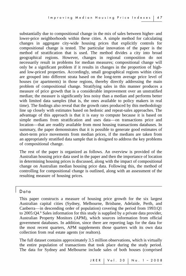
There would, of course, be many other ranking periods that could be used togroup the suburbs into strata based on median prices. For example, the medianprice of suburbs in 1992 could be grouped to form strata for 1993, then the medianprices for 1993 to form strata for 1994, and so on. However, in practice there isa very high degree of stability in the relative price rankings of suburbs: suburbsthat tend to be relatively expensive in one period will tend to be relativelyexpensive 10 years later. Exhibit 6 illustrates this using data for Sydney, showingthat the price relativities in the 2000–2004 sorting period also hold outside thatperiod, and the Spearman rank correlations between median suburb prices inSydney in 1996 and 2004 is 0.95. Similar results hold for other cities, for bothhouses and apartments. Hence, any reasonable alternative price-based strategy forranking suburbs would result in very similar strata, and very similar estimates ofprice growth.

Once suburbs were grouped into deciles (or quintiles), a median price wascalculated for each stratum for each quarter. The changes in the median prices foreach stratum were then weighted together to calculate growth in city-wide prices.There are a number of different weighting schemes that could be used to combinethese ten (or five) growth rates. The simplest method would be to take anunweighted average of the changes. This is equivalent to constructing a city-wide

5 8 � P r a s a d a n d R i c h a r d s

Exhibi t 6 � Median Decile Prices

20052002199919961993

$’000

Sydney houses, log scale, non-seasonally adjusted

$’000

800 800

200 200

100 100

400 400

Note: The lines represent the median price for each of the 10 groups of suburbs in Sydney. The shaded areashows the period used to sort the data. The source is the authors’ analysis using data from APM.

index as the unweighted geometric average of median prices in each stratum.Alternatively, the effect of using weights based on sales volumes over the 12-yearperiod was examined, as were weights based on principal components (wherechanges in prices for any group can be thought as given by an unobservable city-wide movement plus an idiosyncratic component).18

However, different weighting schemes make very little difference to estimates ofshort-term price growth. In the sample, the different weightings yield measures ofquarterly price changes that typically have a correlation of over 0.99. This reflectsthe fact that price changes in the different strata are typically quite highlycorrelated and that in most cases, sales volumes and principal components implyweights for each stratum that are relatively close to equal. Given that equal-weighting produces similar results to other weighting schemes and given that itis the simplest method of weighting the series, all the results shown in subsequentsections of this paper refer to the equally-weighted measure (which is labeled asthe ‘mix-adjusted measure’).

I m p r o v i n g M e d i a n H o u s i n g P r i c e I n d e x e s � 5 9

J R E R � V o l . 3 0 � N o . 1 – 2 0 0 8

� A s s e s s i n g t h e M i x - A d j u s t e d M e a s u r e

The mix-adjusted measure of changes in city-wide house prices was assessed byexamining how well it addressed some of the problems with conventionalunstratified median measures that were highlighted previously. An additionalbenchmark is whether the mix-adjusted measure outperforms the change in aseasonally adjusted median price: this will indicate if the slightly greater datademands of the measure yield a significant improvement relative to accountingfor seasonality in the composition of dwellings sold by just seasonally adjustingmedian prices. In addition, the correlation of the measure is compared withregression-based measures. Some additional perspective is then provided for thereasons for the good performance of the simple measure by comparing it tocommonly used geographic stratification techniques.

Vo l a t i l i t y

Price movements that result from compositional effects can be considered asrepresenting noise that contributes volatility to quarterly price changes rather thanbeing indicative of true price trends in the housing market. To assess how volatiledifferent price series are, the quarterly movements in each of the series iscompared with a measure of the ‘trend’ change in prices.19 A root mean squarederror (RMSE) is then calculated between quarterly growth in each of the measuresand quarterly growth in the trend for each city. Since the trend measure can bethought of as capturing underlying housing price movements (or the cycle), thelarger the deviations from trend, the less informative the series is about theunderlying state of the housing market.

The results in Exhibit 7 indicate that in every case, simply seasonally adjustingthe median price series (using the X12 program) results in a measure of pricechanges that is considerably less volatile than the change in the unadjusted median.However, in every case there is an additional improvement that can be gainedfrom the simple mix-adjusted measure. Taking the reduction in the Australia-widemeasure as a simple metric for the reduction in the proportion of noise in thestandard median, one might conclude that seasonal adjustment can typicallyreduce the extent of noise by nearly 40%, but that the mix-adjusted measure resultsin a more significant reduction, with the average volatility falling by nearly 70%.20

The reduction in volatility is greatest for houses in Sydney and Melbourne. Indeed,it is noteworthy that the average deviation from trend growth in every one of theten deciles (shown in the last column of Exhibit 7) is noticeably smaller than theaverage deviation from trend for the city-wide median. As a further illustration ofthis point, in around half of all quarters in the data sample, the quarterly changein the city-wide median lies outside the range of median price changes in all tendeciles. To be provocative, these results for Sydney and Melbourne suggest that

6 0 � P r a s a d a n d R i c h a r d s

Exhibi t 7 � Volatility in Measures of Changes in Housing Prices

Median(nsa)

Median(sa)

Mix-AdjustedMeasure

Range of RMSEsfor Deciles/Quintiles

Sydney houses 4.04 2.80 1.08 1.41–2.99

Melbourne houses 4.40 2.54 1.40 1.36–3.48

Brisbane houses 1.91 1.61 1.26 1.73–4.88

Perth houses 1.90 1.49 1.07 1.73–3.10

Adelaide houses 2.20 1.37 1.27 1.71–6.07

Canberra houses 2.46 2.41 1.88 2.33–4.78

Sydney apartments 1.93 1.46 1.21 1.60–2.89

Melbourne apartments 3.45 3.01 2.11 2.78–5.59

Australian housing 2.81 1.73 0.88

Note: The sample covers 1993:Q2–2005:Q3. The table shows deviation from trend, quarterlyRMSE in percentage points.

one might get better estimates of the trend in city-wide house prices by lookingat developments in a sample of only about 10% of all sales (albeit a carefullyselected 10%) than from a standard city-wide median using the full sample ofdata.

The gains from stratification will depend on several factors including: the extentof compositional change between higher- and lower-priced properties in each city;the extent of price differences between higher- and lower-priced properties; andthe extent to which the effects of compositional change can be undone via thesuburb-level stratification strategy used here. The reasons for the relatively largerreduction in volatility in house price growth in the two larger cities appear toreflect both a higher degree of compositional change in these two cities (includingthe seasonal component shown in Panel A of Exhibit 4), and greater variation inthe characteristics of the dwelling stock in Sydney and Melbourne (e.g., themedian house price for the tenth decile in Sydney is on average 4.5 times higherthan the median price of the first decile, compared with it being on averagearound 3.2 times higher for most of the other cities). In addition, since the largestcities have more suburbs, it is possible to divide these larger cities into moredifferentiated strata with greater variation in the average prices of suburbs ineach stratum. Hence it would be expected that there would be greater gainsfrom stratification and greater control of compositional change in the largercities.21

I m p r o v i n g M e d i a n H o u s i n g P r i c e I n d e x e s � 6 1

J R E R � V o l . 3 0 � N o . 1 – 2 0 0 8

S e a s o n a l i t y

By construction, the mix-adjusted measure will remove any impact on measuresof price changes that results from seasonality in the composition of sales acrossstrata. However, it will not control for any seasonality from compositional effectswithin strata (e.g., any possible seasonality in the composition of sales betweenthe more and less expensive houses within any suburb). The mix-adjusted measurefor the presence of any residual seasonality was tested to see if seasonality withinstrata is an issue. While median prices in nearly all cities were found to beseasonal, the results (available upon request) indicate that there is no evidence ofidentifiable seasonality in any city, nor at the nationwide level, for the mix-adjusted measure.

C o m p a r i s o n w i t h R e g r e s s i o n - b a s e d M e a s u r e s

One clear advantage of a mix-adjusted measure is the simplicity of its calculation.However, more sophisticated approaches are possible, most notably hedonic andrepeat-sale approaches. Of course these are not without shortcomings: hedonicregressions will only be as good as the data on housing characteristics that areavailable and repeat-sales estimates are likely to have significant problems in realtime and can be subject to non-trivial revisions, given that estimates of pricegrowth in any quarter will be affected by sales that occur in subsequent quarters.

Using Sydney as an example, Exhibit 8 shows quarterly growth in the mix-adjusted measure, along with estimates of growth from hedonic and repeat salesmodels. Growth in the seasonally adjusted and unadjusted median is also shownfor comparison. The hedonic and repeat-sales estimates are taken from Hansen(2006), who uses a dataset virtually identical to the one utilized in this study. Inaddition, quarterly growth in the house price series produced by the nationalstatistical agency, the Australian Bureau of Statistics (ABS), is also shown. TheABS measure is based on purely geographical stratification, using a datasetbroadly similar to the one used in the current study.22 As Exhibit 8 shows, eachof the regression-based measures produces quarterly growth rates that lines upclosely with those from the mix-adjusted measure. There are also noticeabledifferences between estimates of price growth from the city-wide median measuresand the more advanced measures, indicating that it is important to adjust forcompositional effects. Hansen (2006) also provides hedonic and repeat-salesestimates for house price growth in Melbourne and Brisbane. The pattern shownin Exhibit 8 also holds for Melbourne and Brisbane; the more advanced measuresproduce similar estimates of price growth, while growth in the city-wide mediancan diverge significantly from that produced by these measures.

In Exhibit 9, correlation coefficients and a measure of deviations from trend areused to compare quarterly price changes from the mix-adjusted measure toestimates from hedonic and repeat-sales price measures for Sydney, Melbourne,

6 2 � P r a s a d a n d R i c h a r d s

Exhibi t 8 � Quarterly Growth in House Prices

-5

0

5

10

-5

0

5

10

-10

-5

0

5

-10

-5

0

5

Quarterly growth

2005

%Median%

More advanced measures

2002199919961993

%%

Non-seasonally adjustedSeasonally adjusted

Mixed-adjusted HedonicRepeat-sales ABS

Sources: ABS; authors’ calculations using data from APM.

and Brisbane. Panel A of Exhibit 9 indicates that the mix-adjusted measure of thequarterly growth in prices has a high correlation with the regression-basedmeasures: indeed, the mix-adjusted measure tends to have a slightly highercorrelation with each of the regression-based measures than the correlationbetween those more advanced measures. By contrast, the change in the simplemedian often has a fairly modest correlation with the regression-based measures,and seasonal adjustment of the median does not result in any marked increase inthe correlations with the regression-based measures.

Panel B of Exhibit 9 indicates the extent to which each of the measures of houseprice growth deviate from a proxy of underlying house price movements. Thisproxy is obtained by constructing a measure of trend growth for each of the mix-

I m p r o v i n g M e d i a n H o u s i n g P r i c e I n d e x e s � 6 3

J R E R � V o l . 3 0 � N o . 1 – 2 0 0 8

Exhibi t 9 � Correlation between Various House Price Measures

Median(nsa)

Median(sa) Mix-Adjusted Hedonic Repeat-Sales

Panel A: Correlation coefficients, quarterly changes

SydneyMedian (nsa) 1.00Median (sa) 0.77 1.00Mix-adjusted median 0.52 0.65 1.00Hedonic 0.58 0.65 0.97 1.00Repeat-sales 0.38 0.57 0.90 0.89 1.00

MelbourneMedian (nsa) 1.00Median (sa) 0.69 1.00Mix-adjusted median 0.65 0.71 1.00Hedonic 0.66 0.70 0.92 1.00Repeat-sales 0.42 0.57 0.76 0.69 1.00

BrisbaneMedian (nsa) 1.00Median (sa) 0.95 1.00Mix-adjusted median 0.87 0.87 1.00Hedonic 0.89 0.90 0.96 1.00Repeat-sales 0.77 0.81 0.93 0.93 1.00

Panel B: Deviation from trend (quarterly RMSE in percentage points)

Sydney 4.11 2.95 0.97 1.02 0.86Melbourne 4.48 2.64 1.40 1.25 1.57Brisbane 1.96 1.69 1.25 1.25 1.03

Notes: Correlation coefficients and RMSEs across the various measures of quarterly price growthwere calculated over 1993:Q2–2005:Q3. The data vintage used to calculate the hedonic andrepeat-sales measures in Hansen (2006) does not correspond precisely with that used to calculatethe mix-adjusted median here. In addition, Hansen uses data from a different source (the RealEstate Institute of Victoria) to calculate the repeat-sales measure for Melbourne, so the resultsacross measures are not fully comparable for Melbourne.

adjusted, hedonic, and repeat-sales measures (using the moving-average approachoutlined in Endnote 8) and then averaging these three trends. Confirming theearlier results in Exhibit 7, changes in the median and seasonally adjusted medianare quite volatile with relatively high RMSEs. In contrast, the mix-adjustedmeasure and the two regression-based measures provide estimates of underlyinghouse price movements that are comparable in terms of their apparent noise.

It is reassuring that the estimates of the change in house prices derived from themix-adjusted measure are similar to those from regression-based measures,

6 4 � P r a s a d a n d R i c h a r d s

suggesting that simple, but targeted, stratification techniques can control for asignificant proportion of compositional change. However, this result may not beespecially surprising as the measure is conceptually related to a hedonic approachusing location as an explanatory variable. The results in Hansen (2006) indicatethat the vast majority of the explanatory power in standard hedonic regressionscomes from the location of properties, which (in combination with informationon average suburb-level price levels) is the variable used for stratification in themethodology in the current study.

A C o m p a r i s o n w i t h A l t e r n a t i v e P r i c e a n d G e o g r a p h i cS t r a t i f i c a t i o n S t r a t e g i e s

The preceding analysis indicates that the mix-adjusted approach overcomes manyof the problems associated with unstratified median measures. A major reason forthe substantial improvement appears to be the particular method used to stratifytransactions. By stratifying properties on the basis of the median price for theirsuburb, much of the compositional change in sales movements between higher-and lower-priced properties is controlled. However, other stratification strategiesare possible, an obvious alternative being on a broad geographical basis.

Unit record data for Sydney is used to construct two alternative mix-adjustedmeasures of price changes. Two standard geographical classifications for Sydneydivide the city into 49 statistical local areas (SLAs) and 14 statistical subdivisions(SSDs). Measures are constructed using both of these geographic groupings. Toproduce a city-wide measure of price growth, the median house price in eachgeographic region is weighted by the region’s share of sales over the whole sampleperiod. In order to evaluate the relative performance of the geography-basedmeasures of price growth, the deviation (RMSE) of each measure is calculatedfrom the trend growth series used in Panel B of Exhibit 8.

For greater comparability, some alternative price-based mix-adjusted measures arealso constructed. Instead of dividing Sydney into 10 price-based groups, thesuburbs of Sydney are divided into 14 and 49 groups (the same number of groupsas the geographic measures) based on the ranked median price of suburbs over2000–2004. However, to shed further light on the stratification issue, someadditional price-based measures are implemented. In particular, instead of formingmeasures based just on 10, 14, and 49 strata, the robustness of price-basedmeasures is assessed by using everything from 1 stratum (equivalent to the simplecity-wide median) all the way up to 60 strata (each with just 10 or 11 suburbs).

The results are shown in Exhibit 10.23 A first point to note is that price changesestimated from the geographic-based stratifications are less noisy than the simpleunstratified city-wide median. The RMSEs based on the 14 and 49 groups are1.95% and 1.62%, respectively, versus 4.70% for the city-wide median. However,the corresponding price-based stratification measures provide a significantadditional improvement over the geography-based measures, with RMSEs of

I m p r o v i n g M e d i a n H o u s i n g P r i c e I n d e x e s � 6 5

J R E R � V o l . 3 0 � N o . 1 – 2 0 0 8

Exhibi t 10 � Geographic and Price-based Groupings

●

●

●

0

1

2

3

4

0

1

2

3

4

Price-based grouping

60

%%

Deviation from trend, RMSE

50403020100

SSD grouping

SLA grouping

Deviation of the median

Number of groups

Source: Authors’ analysis using data from APM.

1.15% and 1.14%, respectively, for the measures based on 14 and 49 groups. Thisprovides evidence in support of grouping data on the basis of median suburb pricesrather than on a geographic basis, as the former provides a better control forchanges in the mix of sales between more and less expensive properties.

An important additional result in Exhibit 10 concerns the ‘granularity’ ofstratification in the price-based measures. The line on the graph shows how thedeviation from trend (RMSE) varies according to the number of strata used tocalculate price growth. Simply dividing all transactions into two groups of about330 suburbs produces notable gains over the median measure. There are furthersignificant gains from splitting the sample into four groups, but thereafter theRMSE is fairly constant. This implies that one can get fairly comparable estimatesof movements in city-wide house prices by dividing Sydney’s 659 suburbs intoanything from 4 to 60 groups. This result is also confirmed by correlation analysis.Therefore, the results for Sydney shown earlier are not particularly sensitive tothe decision to divide suburbs into 10 groups: indeed, there is a wide range ofprice-based stratification schemes that yield robust results.

6 6 � P r a s a d a n d R i c h a r d s

Therefore, it can be conjectured that the results for the other cities are also notespecially dependent upon the decision to group suburbs into deciles (or quintiles).The objective was not to fit the suburbs in each city into an ‘optimal’ number ofgroups: the choice of deciles was fairly arbitrary, although in cases of smallersample sizes (houses in Canberra, and apartments in Sydney and Melbourne), adecision was made to instead work with quintiles to avoid small sample sizes inparticular strata, especially in the incomplete real-time samples. For otherapplications, there will no doubt be benefits to empirically testing the optimaldegree of stratification, and smaller sample sizes will presumably warrant adifferent number of groups, but the preliminary results here suggest that a rangeof strategies can yield significant benefits over simple medians.24

� C o n c l u s i o n

The conventional wisdom among most housing researchers is that median pricemeasures provide poor measures of the pure price change in the aggregate housingstock, and that regression-based methodologies provide superior measures.25

Yet median price measures are widely cited in the press and are used in a rangeof countries by industry bodies, housing lenders, and sometimes governmentagencies. The reason is presumably that the more advanced techniques requiredetailed data, are typically subject to revision as data for future periods becomeavailable, are less transparent, and require the use of statistical techniques that arenot widely used outside of academic circles.

This study used a dataset of around 3.5 million transactions in Australia’s sixlargest cities to demonstrate that compositional change between higher- and lower-priced parts of cities is a major factor behind the noise in short-term movementsin city-wide median prices. However, the findings show that medians can beconsiderably more reliable if taken from a stratified sample. Given the importanceof location in determining prices, small geographic regions are grouped accordingto the long-term average price of dwellings in those regions, rather than simplyclustering smaller geographic regions into larger geographic regions. Therefore,the method of stratification directly controls for what appears to be the mostimportant form of compositional change: changes in the proportion of houses soldin higher- and lower-priced regions in any period. Stratifying sales in this mannerproduces a mix-adjusted measure of price growth that substantially improves uponstandard unstratified median measures. In particular, the mix-adjusted measure ofprice growth is considerably less volatile and not subject to seasonality. Inaddition, it is highly correlated with estimates of price growth from measuresbased on regression-based approaches.

The choice between different methodologies for estimating changes in aggregateprices will always involve a trade-off between various competing concernsincluding the ease of construction, the extensiveness of data requirements, and theextent to which the methodology controls for quality (see also Bourassa, Hoesli,and Sun, 2006). Given the recent sharp run-up in house prices in many countries,

I m p r o v i n g M e d i a n H o u s i n g P r i c e I n d e x e s � 6 7

J R E R � V o l . 3 0 � N o . 1 – 2 0 0 8

one particular concern will be timeliness, especially for macroeconomicpolicymakers. However, one problem in this regard is that the groups with thebest access to timely data are often industry or government bodies, which may beunable or unwilling to use the more sophisticated methodologies. This highlightstwo particular advantages with the approach proposed in this paper. First, themethod used to control for compositional change is computationally simple,requiring nothing more than the use of a ‘sort’ command. Furthermore, theapproach does not require the use of databases that contain a large amount ofinformation on housing characteristics. It uses variables—transactions price andlocation—that are readily available from most housing transactions databases.The approach has now been used successfully in Australia for more than a yearand a half, with good estimates of quarterly price changes feasible even withincomplete and biased initial samples.26 Accordingly, the methodology outlined inthis paper may be applicable for measuring house price growth in other countriesas well.

� E n d n o t e s1 There is, for example, a significant literature on the question of whether central banks

should ‘lean against’ perceived bubbles in asset markets by tightening policy, thoughthere is reasonably general consensus that the conditions for such action will notgenerally be met (e.g., Gruen, Plumb, and Stone, 2005).

2 For example, Bourassa, Hoesli, and Sun (2006, p. 81) put it this way: ‘‘Despite the factthat median house price indexes are widely available in several countries, they are proneto severe biases due to the heterogeneity of properties. Stated differently, such methodsare unable to distinguish between movements in prices and changes in the compositionof dwellings sold from one period to the next.’’

3 For more information on repeat sales, see Case and Shiller (1987). An early referenceto the theory underlying hedonic models is Rosen (1974). There are also numerousarticles comparing the two methodologies, for example Haurin and Hendershott (1991),Crone and Voith (1992), and Meese and Wallace (1997).

4 For example, see Clapp, Giaccotto, and Tirtiroglu (1991) and Clapham, Englund,Quigley, and Redfearn (2006) for evidence on the significant revisions to repeat salesestimates and the sometimes poor performance in estimating short-term price changes.

5 For example, the U.S. National Association of Realtors release their monthly price seriesaround 31⁄2 weeks after the end of the month, whereas the OFHEO quarterly repeatsales index is released about nine weeks after the end of the relevant quarter (althoughthere are instances in some other countries where indices using more sophisticatedmethodologies are released prior to median price series).

6 Other papers that construct housing price indexes for Australia include Bourassa andHendershott (1995), Rossini (2000), ABS (2005), and Hansen (2006).

7 Through the rest of the paper, all calculations involving changes in prices use the changein the log of the price series. In cases where these are shown in a table or graph, theyare the log change multiplied by 100 so as to correspond approximately to percentagechanges.

6 8 � P r a s a d a n d R i c h a r d s

8 The trend is calculated as the change in the five-quarter-centred moving average of (thelog of) the median price series. The weights in the moving average are 0.125, 0.25,0.25, 0.25, and 0.125, which should remove any seasonality from the trend.

9 There appears to be a downward trend in this ratio over the sample, perhaps becausethe growth in the city has been in suburbs relatively far from the center, which tend tobe less expensive suburbs.

10 The compositional change variable has also been regressed on the three measures ofpure price changes outlined in the second half of this paper. The results indicate thatthere is no tendency for compositional change to be related to ‘true’ changes in houseprices, so the results in Exhibit 3 reflect spurious compositional effects on median prices.

11 The U.S. Census Bureau’s X12 seasonal adjustment program decomposes a series intoits trend-cycle, seasonal, and irregular components and provides tests for stableseasonality (whether or not seasonal factors have an effect on the series) and movingseasonality (whether or not the seasonal pattern changes from year to year).

12 It is beyond the scope of this paper to consider the reasons for the seasonality in thecomposition of sales. However, in those cities where sales volumes are found to beseasonal, the seasonality comes more from variation in the sales volumes in higher-priced suburbs than in lower-priced suburbs. This would be consistent with some citieshaving particular ‘selling seasons,’ especially in higher-priced suburbs.

13 The series for the U.S., Canada, and New Zealand refer to existing one-family homes,dwellings, and existing dwellings, respectively. The analysis uses data for 1975:Q2–2005:Q4 for the U.S., 1980:Q1–2005:Q4 for Canada, and 1992:Q1–2005:Q4 for NewZealand. The U.S. data have been converted to a quarterly series by averaging themonthly series.

14 For example, the National Association of Realtors report on existing home sales inSeptember 2004 notes that: ‘‘Most families with children, who typically buy moreexpensive homes, time their purchase based on school year considerations.’’ In addition,the Real Estate Institute of New Zealand’s Residential Market News report for March2005 noted that: ‘‘A switch to higher end market residential property sales saw theresidential property median price rise.’’

15 This is consistent with work by Jud and Seaks (1994) using U.S. data that shows thatsignificant differences in estimated price growth can result when Heckman’s two-stageestimation procedure is used to account for potential problems in sample selectivity inthe transactions that are observed.

16 In addition to location, most measures that use stratification also group transactionsaccording to dwelling type. As well as the measures in the table, a number of countriesin continental Europe (including Austria, Finland, Hungary, and Portugal) make arudimentary adjustment for quality by measuring prices in per square meter terms.Beyond this, most measures do not control for quality. This is probably because manydatasets do not contain comprehensive information on dwelling characteristics.

17 Further, natural boundaries will sometimes hinder the formation of larger homogenousgroups. For example, expensive houses in a city may be clustered around a harbor oron either side of a river, but such natural barriers will often be used to divide the cityinto different geographic regions.

18 Alternatively, if the intention is to measure changes in the value of the housing stock,suburb-level dwelling stock weights will be most appropriate.

19 The trend is calculated using the moving-average approach described in Endnote 8. Twomeasures of trend are constructed first: one from an index version of the mix-adjusted

I m p r o v i n g M e d i a n H o u s i n g P r i c e I n d e x e s � 6 9

J R E R � V o l . 3 0 � N o . 1 – 2 0 0 8

measure and the other using the seasonally adjusted median. The measure of trend usedin the comparison in Exhibit 7 is the average of the growth rates of the two smoothedmeasures so as to ensure a fair ‘horse race’ between the measure and the seasonallyadjusted measure (though the results are not sensitive to the precise calculation of trendgrowth).

20 An alternative comparison is shown in the working paper version of this paper: for thenationwide price measure, the standard deviation of the mix-adjusted measure is 42%below that of the unadjusted median measure. Stephens, Li, Lekkas, Abraham, Calhoun,and Kimner (1994) do a related comparison of the reduction in standard deviation fromthe U.S. OFHEO repeat sales measure relative to the National Association of Realtorsmedian measure: across their 11 cities, the median reduction is also 42%.

21 Using unit record data for Sydney, the mix-adjusted measure is found to perform betterin real time when compared with an unadjusted median. The real time data problem inAustralia results from the existence of a lag between when a sale is agreed to and whenthis sale becomes recorded in a housing transactions database. Therefore initial estimatesof price growth in any quarter are based on only a small sample of all transactions thatwill eventually be available for that quarter. Comparing an ‘initial’ estimate of pricegrowth made with the data available one month after the end of a quarter, with thatmade from the latest vintage of data, the growth in the standard city-wide median isfound to be revised by around 7.5 percentage points on average, compared with aconsiderably smaller 1.5 percentage point revision for the mix-adjusted measure.

22 The ABS measure is only shown from 2002 when there is a series break andmethodological improvements to the measure (see ABS 2005).

23 Due to some constraints in the unit record data, the results here differ somewhat fromthe results in Exhibits 7 and 9. The measures in this section are constructed using unitrecord data that are of a different vintage and cover a different time span (1996:Q1–2005:Q3) to the data used in the rest of the paper.

24 See Hansen, Hurwitz, and Madow (1953) and Everitt (1980) for more information onthe theoretical issues in the optimal grouping of data.

25 Some researchers (e.g., Gatzlaff and Ling, 1994; and Meese and Wallace 1997) havenoted, however, that median price measures provide reasonably satisfactory measures oflong-term price trends, and others (e.g., Crone and Voith, 1993) have sometimes foundbig differences between results from more sophisticated measures.

26 The methodology is now used by Australian Property Monitors (www.apm.com.au).

� R e f e r e n c e s

Australian Bureau of Statistics (ABS). Renovating the Established House Price Index. ABSInformation Paper No. 6417.0, 2005.

Berg, L. Price Indexes for Multi-Dwelling Properties in Sweden. Journal of Real EstateResearch, 2005, 27:1, 47–81.

Bourassa, S.C. and P.H. Hendershott. Australian Capital City Real House Prices, 1979–1993. Australian Economic Review, 1995, 28:3, 16–26.

Bourassa S.C., E. Cantoni, and M. Hoesli. Spatial Dependence, Housing Submarkets, andHouse Prices. FAME Research Paper Series No. 151, 2005.

Bourassa, S.C., M. Hoesli, and J. Sun. A Simple Alternative House Price Index Method.Journal of Housing Economics, 2006, 15:1, 80–97.

7 0 � P r a s a d a n d R i c h a r d s

Can, A. GIS and Spatial Analysis of Housing and Mortgage Markets. Journal of HousingResearch, 1998, 9:1, 61–86.

Can, A. and I.F. Megbolugbe. Spatial Dependence and House Price Index Construction.Journal of Real Estate Finance and Economics, 1997, 14:1, 203–22.

Case, K.E. and R.J. Shiller. Prices of Single-Family Homes since 1970: New Indexes forFour Cities. New England Economic Review, 1987, September/October, 45–56.

Clapham, E., P. Englund, J.M. Quigley, and C.L. Redfearn. Revisiting the Past and Settlingthe Score: Index Revision for House Price Derivatives. Real Estate Economics, 2006, 34:2, 275–302.

Clapp, J.M., C. Giaccotto, and D. Tirtiroglu. Housing Price Indices Based on allTransactions Compared to Repeat Subsamples. Journal of the American Real Estate andUrban Economics Association, 1991, 19:3, 270–85.

Crone, T.M. and R.P. Voith. Estimating House Price Appreciation: A Comparison ofMethods. Journal of Housing Economics, 1993, 2:4, 324–38.

Everitt, B. Cluster Analysis. Second edition. New York: Social Science Research Councilby Heinemann Educational Books, Halstead Press, 1980.

Gatzlaff, D.H. and D.C. Ling. Measuring Changes in Local House Prices: An EmpiricalInvestigation of Alternative Methodologies. Journal of Urban Economics, 1994, 35:2, 221–44.

Goodman, A.C. and T.G. Thibodeau. Housing Market Segmentation and HedonicPrediction Accuracy. Journal of Housing Economics, 2003, 12:3, 181–201.

Gruen, D., M. Plumb, and A. Stone. How Should Monetary Policy Respond to Asset-PriceBubbles. International Journal of Central Banking, 2005, 1:3, 1–31.

Hansen, J. Australian House Prices: A Comparison of Hedonic and Repeat-Sales Measures.Reserve Bank of Australia Research Discussion Paper No 2006-03, 2006.

Hansen, M.H., W.N. Hurwitz, and W.G. Madow. Sample Survey Methods and Theory:Volume I, New York: Wiley, 1953.

Haurin, D.R. and P.D. Hendershott. House Price Indexes: Issues and Results. Journal ofthe American Real Estate and Urban Economics Association, 1991, 19:3, 259–69.

Jud, G.D. and T.G. Seaks. Sample Selection Bias in Estimating Housing Sales Prices.Journal of Real Estate Research, 1994, 9:3, 289–98.

Lavallee, P. Two-Way Optimal Stratification Using Dynamic Programming. Proceedings ofthe Survey Methods Section. Eleventh edition. American Statistics Association, Alexandria,1988, 646–51.

Meese, R.A. and N.E. Wallace. The Construction of Residential Housing Price Indices: AComparison of Repeat-Sales, Hedonic-Regression, and Hybrid Approaches. Journal of RealEstate Finance and Economics, 1997, 14:1–2, 51–73.

Rosen, S., Hedonic Price and Implicit Markets: Product Differentiation in PureCompetition, Journal of Political Economy, 1974, 82(1), 34–55.

Rossini, P., Estimating the Seasonal Effects of Residential Property Markets—A CaseStudy of Adelaide. Paper presented at Sixth Annual Pacific-Rim Real Estate SocietyConference, Sydney, January 24–27, 2000.

Stephens, W., Y. Li, V. Lekkas, J. Abraham, C. Calhoun, and T. Kimner. ConventionalMortgage Home Price Index. Journal of Housing Research, 1995, 6:3, 389–418.

Straszheim, M.R. An Econometric Analysis of the Urban Housing Market. New York:National Bureau of Economic Research, 1975.

I m p r o v i n g M e d i a n H o u s i n g P r i c e I n d e x e s � 7 1

J R E R � V o l . 3 0 � N o . 1 – 2 0 0 8

The views expressed in this paper are those of the authors and should not be attributedto the Reserve Bank of Australia. We thank Steven Bourassa, Luci Ellis, James Hansen,James Holloway, Christopher Kent, Kristoffer Nimark, and an anonymous referee forhelpful comments. Thanks also to Australian Property Monitors, and in particularLouis Christopher, for compiling the raw data used in this paper.

Nalini Prasad, Reserve Bank of Australia, NSW, Australia 2001 or prasadn@rba.gov.au.

Anthony Richards, Reserve Bank of Australia, NSW, Australia 2001 or richardsa@rba.gov.au.