Utah State University Utah State University

DigitalCommons@USU DigitalCommons@USU

All Graduate Theses and Dissertations Graduate Studies

8-2021

Deep Learning Data and Indexes in a Database Deep Learning Data and Indexes in a Database

Vishal Sharma Utah State University

Follow this and additional works at: https://digitalcommons.usu.edu/etd

Part of the Databases and Information Systems Commons

Recommended Citation Recommended Citation Sharma, Vishal, "Deep Learning Data and Indexes in a Database" (2021). All Graduate Theses and Dissertations. 8214. https://digitalcommons.usu.edu/etd/8214

This Dissertation is brought to you for free and open access by the Graduate Studies at DigitalCommons@USU. It has been accepted for inclusion in All Graduate Theses and Dissertations by an authorized administrator of DigitalCommons@USU. For more information, please contact digitalcommons@usu.edu.

DEEP LEARNING DATA AND INDEXES IN A DATABASE

by

Vishal Sharma

A dissertation submitted in partial fulfillmentof the requirements for the degree

of

DOCTOR OF PHILOSOPHY

in

Computer Science

Approved:

Curtis Dyreson, Ph.D. Nicholas Flann, Ph.D.Major Professor Committee Member

Vladimir Kulyukin, Ph.D. Kevin R. Moon, Ph.D.Committee Member Committee Member

Haitao Wang, Ph.D. D. Richard Cutler, Ph.D.Committee Member Interim Vice Provost of Graduate Studies

UTAH STATE UNIVERSITYLogan, Utah

2021

ii

Copyright © Vishal Sharma 2021

All Rights Reserved

iii

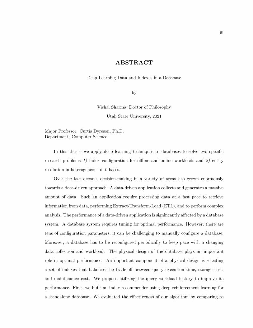
ABSTRACT

Deep Learning Data and Indexes in a Database

by

Vishal Sharma, Doctor of Philosophy

Utah State University, 2021

Major Professor: Curtis Dyreson, Ph.D.Department: Computer Science

In this thesis, we apply deep learning techniques to databases to solve two specific

research problems 1) index configuration for offline and online workloads and 2) entity

resolution in heterogeneous databases.

Over the last decade, decision-making in a variety of areas has grown enormously

towards a data-driven approach. A data-driven application collects and generates a massive

amount of data. Such an application require processing data at a fast pace to retrieve

information from data, performing Extract-Transform-Load (ETL), and to perform complex

analysis. The performance of a data-driven application is significantly affected by a database

system. A database system requires tuning for optimal performance. However, there are

tens of configuration parameters, it can be challenging to manually configure a database.

Moreover, a database has to be reconfigured periodically to keep pace with a changing

data collection and workload. The physical design of the database plays an important

role in optimal performance. An important component of a physical design is selecting

a set of indexes that balances the trade-off between query execution time, storage cost,

and maintenance cost. We propose utilizing the query workload history to improve its

performance. First, we built an index recommender using deep reinforcement learning for

a standalone database. We evaluated the effectiveness of our algorithm by comparing to

iv

several state-of-the-art approaches. Second, we develop a real-time index recommender

that can, in real-time, dynamically create and remove indexes for better performance in

response to sudden changes in the query workload. Third, we develop a database advisor.

Our advisor framework will be able to learn hidden patterns from a workload. It can

enhance a query, recommend interesting queries, and summarize a workload.

The entity resolution problem is to match entities from heterogeneous databases. With

the emergence of massive amount of data, linking data between data collections, known as

entity resolution, has become very important. We build a system to link social media

profiles from three popular social media networks. Our system, called LinkSocial , is fast,

scalable and accurate.

Overall, this thesis provides evidence for two statements 1) using a historical SQL

workload, a database can be optimized autonomously with high accuracy, 2) using basic

features from social media, user entities can be effectively linked across multiple social media

platforms.

(73 pages)

v

PUBLIC ABSTRACT

Vishal Sharma

A database is used to store and retrieve data, which is a critical component for anysoftware application. Databases requires configuration for efficiency, however, there are tensof configuration parameters. It is a challenging task to manually configure a database. Fur-thermore, a database must be reconfigured on a regular basis to keep up with newer dataand workload. The goal of this thesis is to use the query workload history to autonomouslyconfigure the database and improve its performance. We achieve proposed work in fourstages: (i) we develop an index recommender using deep reinforcement learning for a stan-dalone database. We evaluated the effectiveness of our algorithm by comparing with severalstate-of-the-art approaches, (ii) we build a real-time index recommender that can, in real-time, dynamically create and remove indexes for better performance in response to suddenchanges in the query workload, (iii) we develop a database advisor. Our advisor frameworkwill be able to learn latent patterns from a workload. It is able to enhance a query, rec-ommend interesting queries, and summarize a workload, (iv) we developed LinkSocial , afast, scalable, and accurate framework to gain deeper insights from heterogeneous data.

vi

To my friends and family

vii

ACKNOWLEDGMENTS

Academically and personally, the journey of PhD has been an excellent learning curve.

I would like to thank my advisor Dr. Curtis Dyreson for helping me throughout this journey.

I am grateful for his unwavering encouragement and empathy with a beginner like me, as

well as his ability to listen, assist, and answer all of my questions. I’d like to express my

gratitude for his financial assistance.

I’d like to express my gratitude to Dr. Nicholas Flann, Dr. Vladimir Kulyukin, Dr.

Kevin R. Moon, and Dr. Haitao Wang for serving on my graduate committee and for their

help and valuable suggestions during my time at Utah State University. I’d also like to

express my gratitude to USU’s CSE Department for their support. I’d like to express my

gratitude to all of my friends and family for their motivation during this journey.

viii

CONTENTS

Page

ABSTRACT . . . . . . . . . . . . . . . . . . . . . . . . . . . . . . . . . . . . . . . . . . . . . . . . . . . . . . iii

PUBLIC ABSTRACT . . . . . . . . . . . . . . . . . . . . . . . . . . . . . . . . . . . . . . . . . . . . . . . v

ACKNOWLEDGMENTS . . . . . . . . . . . . . . . . . . . . . . . . . . . . . . . . . . . . . . . . . . . . vii

LIST OF TABLES . . . . . . . . . . . . . . . . . . . . . . . . . . . . . . . . . . . . . . . . . . . . . . . . . x

LIST OF FIGURES . . . . . . . . . . . . . . . . . . . . . . . . . . . . . . . . . . . . . . . . . . . . . . . . xi

CHAPTER

1 INTRODUCTION . . . . . . . . . . . . . . . . . . . . . . . . . . . . . . . . . . . . . . . . . . . . . . . 11.1 Outline of Thesis . . . . . . . . . . . . . . . . . . . . . . . . . . . . . . . . . 21.2 Database Index Recommendation . . . . . . . . . . . . . . . . . . . . . . . . 31.3 Entity Resolution in Heterogeneous Databases . . . . . . . . . . . . . . . . 91.4 Overall Contributions . . . . . . . . . . . . . . . . . . . . . . . . . . . . . . 11

2 LINKSOCIAL: Linking User Profile Across Multiple Social Media Platforms . . . . . 132.1 Introduction . . . . . . . . . . . . . . . . . . . . . . . . . . . . . . . . . . . . 142.2 Motivation . . . . . . . . . . . . . . . . . . . . . . . . . . . . . . . . . . . . 152.4 Problem Definition . . . . . . . . . . . . . . . . . . . . . . . . . . . . . . . . 162.5 The LinkSocial Framework . . . . . . . . . . . . . . . . . . . . . . . . . . 162.6 Experiments . . . . . . . . . . . . . . . . . . . . . . . . . . . . . . . . . . . . 182.7 Related Works . . . . . . . . . . . . . . . . . . . . . . . . . . . . . . . . . . 202.8 Conclusion . . . . . . . . . . . . . . . . . . . . . . . . . . . . . . . . . . . . 21

3 MANTIS: Multiple Type and Attribute Index Selection using Deep ReinforcementLearning . . . . . . . . . . . . . . . . . . . . . . . . . . . . . . . . . . . . . . . . . . . . . . . . . . . . . . . . . 22

3.1 Introduction . . . . . . . . . . . . . . . . . . . . . . . . . . . . . . . . . . . . 233.2 Related Work . . . . . . . . . . . . . . . . . . . . . . . . . . . . . . . . . . . 253.3 Problem Formulation . . . . . . . . . . . . . . . . . . . . . . . . . . . . . . . 263.4 MANTIS Framework . . . . . . . . . . . . . . . . . . . . . . . . . . . . . . . 273.5 Experimental Setup . . . . . . . . . . . . . . . . . . . . . . . . . . . . . . . 303.6 Results . . . . . . . . . . . . . . . . . . . . . . . . . . . . . . . . . . . . . . . 333.7 Conclusion and Future Work . . . . . . . . . . . . . . . . . . . . . . . . . . 34

4 Indexer++: Workload-Aware Online Index Tuning Using Deep Reinforcement Learn-ing . . . . . . . . . . . . . . . . . . . . . . . . . . . . . . . . . . . . . . . . . . . . . . . . . . . . . . . . . . . . . 37

4.1 Introduction . . . . . . . . . . . . . . . . . . . . . . . . . . . . . . . . . . . . 384.2 Related Work . . . . . . . . . . . . . . . . . . . . . . . . . . . . . . . . . . . 394.3 Problem Formulation . . . . . . . . . . . . . . . . . . . . . . . . . . . . . . . 39

ix

4.4 Indexer++ . . . . . . . . . . . . . . . . . . . . . . . . . . . . . . . . . . . . 404.5 Experiments . . . . . . . . . . . . . . . . . . . . . . . . . . . . . . . . . . . . 444.6 Conclusion and Future Work . . . . . . . . . . . . . . . . . . . . . . . . . . 48

5 Conclusion and Future Work . . . . . . . . . . . . . . . . . . . . . . . . . . . . . . . . . . . . . . . 51

REFERENCES . . . . . . . . . . . . . . . . . . . . . . . . . . . . . . . . . . . . . . . . . . . . . . . . . . . 52

x

LIST OF TABLES

Table Page

2.1 Number of profiles obtained per social media platform . . . . . . . . . . . . 16

2.2 Number of users with profile on pair-wise and multi-platforms . . . . . . . . 16

2.3 Comparison with previous research . . . . . . . . . . . . . . . . . . . . . . . 18

2.4 LinkSocial performance on pair-wise UPL . . . . . . . . . . . . . . . . . . 19

2.5 LinkSocial performance on multi-platform UPL . . . . . . . . . . . . . . . 19

2.6 Reported accuracy from few previous work . . . . . . . . . . . . . . . . . . 19

4.1 IMDB Dataset Queries . . . . . . . . . . . . . . . . . . . . . . . . . . . . . . 47

4.2 TPC-H Random Dataset Queries . . . . . . . . . . . . . . . . . . . . . . . . 47

4.3 IMDB Queries with no SQL Keyword . . . . . . . . . . . . . . . . . . . . . 47

4.4 TPC-H Random Dataset with no SQL Keyword . . . . . . . . . . . . . . . 47

4.5 Average accuracy from both datasets . . . . . . . . . . . . . . . . . . . . . . 47

xi

LIST OF FIGURES

Figure Page

1.1 Artificial Intelligence applied to different areas of databases . . . . . . . . . 3

2.1 LinkSocial Framework . . . . . . . . . . . . . . . . . . . . . . . . . . . . . 15

2.2 Missing profile information on various social media platforms . . . . . . . . 15

2.3 Bathymetry of the Discovery Transform Fault . . . . . . . . . . . . . . . . . 17

2.4 Comparison of cluster size to accuracy on train data . . . . . . . . . . . . . 18

2.5 Partial dependence plots for individual features . . . . . . . . . . . . . . . . 20

3.1 Figure(a) shows number of parameters in Postgres (2000-2020). Figure(b)shows effect on a workload performance using different parameter settings . 24

3.2 MANTIS Framework . . . . . . . . . . . . . . . . . . . . . . . . . . . . . . . 28

3.3 Power Throughput and QphH values of index recommendation methods andthere comparison in different scenarios on TPC-H dataset . . . . . . . . . . 32

3.4 Workload execution cost with respect to selected indexes on IMDB dataset 33

3.5 Power Throughput and QphH values of index recommendation methods andthere comparison in different scenarios on IMDB dataset . . . . . . . . . . . 34

4.1 Indexer++ Framework . . . . . . . . . . . . . . . . . . . . . . . . . . . . . . 40

4.2 Configuration of trigger parameters λ and Diff(W1W2) . . . . . . . . . . . 41

4.3 Workload Trend Detection on three groups of TPC-H Random dataset wherered circle indicates the centroid of the cluster. (figure is better viewed in color) 42

4.4 Workload Trend Detection on TPC-H dataset. It is a scenario when no re-configurations of indexes is trigger. The new queries are similar to existingworkload. The red circle indicates the centroid of the cluster. The existingworkload is displayed in orange and new queries are in gray. (figure is betterviewed in color) . . . . . . . . . . . . . . . . . . . . . . . . . . . . . . . . . . 42

4.5 A robot navigation in a warehouse from a start point (in red) to end point(in green) blue boxes show an optimal route and gray boxes are obstacles(better view in color) . . . . . . . . . . . . . . . . . . . . . . . . . . . . . . . 44

xii

4.6 TPC-H Template TPC-H Random and IMDB workload representation. Thenumeric value represent serial number. . . . . . . . . . . . . . . . . . . . . . 48

4.7 TPC-H Template TPC-H Random and IMDB workload representation withno keywords. The numeric value represent serial number. . . . . . . . . . . 48

4.8 Cumulative Rewards by DQN agent on IMDB dataset. The dataset is intro-duced in three stages starting with Group 1 as initial workload then Group2 and 3. . . . . . . . . . . . . . . . . . . . . . . . . . . . . . . . . . . . . . . 48

4.9 Cumulative Rewards by DQN agent on IMDB dataset. The dataset is intro-duced in three stages starting with Group 1 as initial workload then combinedwith Group 2 and 3. . . . . . . . . . . . . . . . . . . . . . . . . . . . . . . . 48

CHAPTER 1

INTRODUCTION

Organizations use databases to manage data; for instance, banks store financial data in

databases, marketplaces use databases for tracking products, and scientists deposit knowl-

edge gleaned from experiments in databases. Databases are widely used because they

support efficient querying and updating by multiple users.

Traditionally, a machine learning technique was used to acquire patterns from the

dataset. A machine learning algorithm learns a mapping from given input data to an

output. This approach has limitations concerning the representation of data. The Deep

Learning technique solves this problem by learning to represent data and map an input to

the output. The learned representation usually outperforms traditional handcrafted fea-

tures. Deep Learning is also known as representation learning. Deep Learning has been

previously used to solve many problems and has been applied to almost every research

domain, e.g., Biology, Economics, Engineering, etc. Such representation learning has also

gained significant research development in the field of Computer Vision and Natural Lan-

guage Processing. The research and practice in databases have also been influenced by deep

learning. Deep learning has been used for buffer size tuning [1], learning index structure [2],

data layout partitioning [3], join order selection [4].

Deep Learning techniques have been previously applied to databases. For instance, it

has been applied to tune buffer size tuning [1], learning indexes [2], improve data layout

partitioning [3], and reorder joins [4]. A recent survey of literature in the field [5] organized

the application of deep learning into four broad categories: (1) knob tuning (2) optimization

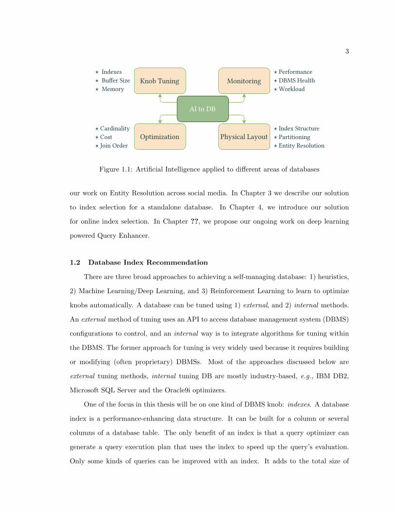
(3) monitoring, and (4) learning physical layout. These categories are depicted in Figure 1.1.

Knob tuning the process of adjusting database parameters, such as buffer size, to optimize

performance. The problem is complex because a database has many tens of parameters

2

that can be tuned. Monitoring is keeping track of how the health of a database, e.g.,

throughput, latency, memory use, changes over time, and tuning knobs as needed to ensure

continued good health. Optimization is learning how to improve query performance. Query

optimization needs to estimate the size of intermediate query results, decide when to use an

index to improve a query and explore the space of query execution plans to choose an optimal

plan. Finally, physical layout refers to how the data is organized in storage, either on disk or

sharded in a cloud computing architecture. In terms of traditional database problems, index

selection, buffer size recommendation, and workspace memory allocation are knob tuning

types of problem. Database performance management, the health of a DBMS, and workload

analysis can be categorized as monitoring problems. Estimating database cardinality, query

cost, and join order selection is classified as optimization problems. Learning an index

structure, table partitioning, and linking data from sources are categorized as learning a

database’s physical layout.

In this proposal, we focus on three different categories of database improvement using

deep learning:

• Knob Tuning : We propose an index recommendation framework using Deep Re-

inforcement Learning for an offline(standalone: RL Index) and online (streaming:

Indexer++) workload.

• Physical Layout : We propose a LinkSocial framework for an entity linkage using

deep learning in a heterogeneous database.

• Monitoring : We propose QueryEnhancer a deep learning powered database workload

analyzer.

1.1 Outline of Thesis

In the remainder of Chapter 1, we describe the index recommendation problem and

related works in more detail in Section 1.2. We then describe Entity Resolution problem in

Section 1.3 and propose our overall contribution in Section 1.4. In Chapter 2 we describe

3

AI to DB

Knob Tuning

Optimization Physical Layout

Monitoring  Indexes   Buffer Size   Memory

  Cardinality  Cost  Join Order

  Index Structure  Partitioning  Entity Resolution

  Performance  DBMS Health  Workload

Figure 1.1: Artificial Intelligence applied to different areas of databases

our work on Entity Resolution across social media. In Chapter 3 we describe our solution

to index selection for a standalone database. In Chapter 4, we introduce our solution

for online index selection. In Chapter ??, we propose our ongoing work on deep learning

powered Query Enhancer.

1.2 Database Index Recommendation

There are three broad approaches to achieving a self-managing database: 1) heuristics,

2) Machine Learning/Deep Learning, and 3) Reinforcement Learning to learn to optimize

knobs automatically. A database can be tuned using 1) external, and 2) internal methods.

An external method of tuning uses an API to access database management system (DBMS)

configurations to control, and an internal way is to integrate algorithms for tuning within

the DBMS. The former approach for tuning is very widely used because it requires building

or modifying (often proprietary) DBMSs. Most of the approaches discussed below are

external tuning methods, internal tuning DB are mostly industry-based, e.g., IBM DB2,

Microsoft SQL Server and the Oracle9i optimizers.

One of the focus in this thesis will be on one kind of DBMS knob: indexes. A database

index is a performance-enhancing data structure. It can be built for a column or several

columns of a database table. The only benefit of an index is that a query optimizer can

generate a query execution plan that uses the index to speed up the query’s evaluation.

Only some kinds of queries can be improved with an index. It adds to the total size of

4

a database. Database indexes are critical to optimizing query workloads. They are very

efficient in locating and accessing data. Out of several parameters, database indexes are

among the most time-consuming and impacting parameters for a workload performance [6].

In this thesis, one of the problems we address is index recommendation in a database. An

approach that is effective and practical in the real world. In the next few sections, we

explore previous work, their limitations, and propose our contribution.

1.2.1 Previous Work

Tuning Based on Heuristics

The idea of a self-managing database based on heuristics dates back to the 1970s

when a self-adaptive physical database design was proposed [7]. This idea was extended

by introducing a heuristic algorithm for index selection [8] and attribute partitioning [9]

in a self-adaptive DBMS. In 1992, an adaptive and automatic index selection was pro-

posed based on query workload statistics [10]. Two years later, the COMFORT online

automatic tuning project was described, it had performance load tuning and a self-tuning

buffering method [11]. In the late 1990s, several enhancements were made in Microsoft’s

SQL server with automatic index selection [12] and physical design tuning wizard [13]. By

early 2000, IBM’s DB2 was equipped with better API support which led to several new

areas of database tuning [14] for instance buffer pool size selection [15], index selection [16],

automatic physical database design [17], adaptive self-tuning memory heaps and database

memory allocation [18]. Self-tuning architectures were also proposed by Oracle in 9i and

10g DBMS [19,20].

The methods used to tune DMBS during these years were based on either heuristics

(hard-coded rules) or cost-based optimization (greedy approach, genetic algorithms) [21].

Both approaches have limitations, heuristics can not generalize a problem, and cost-based

optimization is very cost-ineffective. These techniques are also an offline mode of training

where they do not consider previously tuned configuration for the next tuning/online tuning.

5

Tuning Based on Machine Learning

During the 2010s, Machine Learning techniques have been widely used for optimizing

DBMSs. Aken et al. [22], utilizes both supervised and unsupervised machine learning

for recommending knob configurations. They identify the essential knobs using Lasso,

categorize workload using K-means clustering and recommend knob setting in both online

and offline settings [23]. Kraska et al. [24] proposed SageDB, a new DBMS system capable

of learning the structure of data and providing optimal query plans. Recursive model indexes

(RMI) [2] learn indexes for efficient data access and perform better than traditional B-tree

indexes. They also propose smarter query execution plans to take advantage of GPUs/TPUs

for computation. Kossmann and Schlosser [25] proposed a component (workload analyzer,

tuner, organizer) based modular framework for self-managing databases. They use cost-

effective Linear Programming (LP) algorithms to solve optimization problems. Pavlo et al.

[26] proposed a self-managing database built from scratch with fully autonomous operation

capability. Ding et al. [27] used Neural Network for a better query cost estimation and

used the estimates for index recommendation. Finally, Neuhaus proposed using a genetic

algorithm for optimization and index selection et al. [28].

Machine Learning-based tuning has a weakness in that they require enormous data and

massive computation power to be effective. Such systems can perform great in a controlled

environment, but they have minimal use in real-time scenarios. With these limitations of

heuristics and Machine Learning approaches, we move to our third approach, which has not

been explored.

Tuning Based on Reinforcement Learning

In recent years, Reinforcement Learning (RL) has become popular technique for combi-

natorial optimization. It has been used in several optimization problems in databases such

as optimizing join order [4,29,30], query optimization [31–34], self-tuning databases [35,36]

and data partitioning [3, 37, 38]. For the index selection problem, Basu et al. [39], pro-

posed a tuning strategy using Reinforcement Learning. They formulated index selection

as a Markovian Decision Process and used a state-space reduction technique to help scale

6

their algorithm for larger databases and workloads. Sharma et al. [40] proposed NoDBA

for index selection. They use a given workload (Iworload) and potential indexes (Iindexes)

stacked as input to the neural network. Specifically, they use Deep Reinforcement Learning

with a custom reward function. Their actions include only single indexes that make this

approach faster but unable to learn multi-column indexes. Welborn et al. [41], introduced

latent space representation for workload and action spaces calling it the Structured Action

Space. This representation enables them to perform other tasks as well, e.g., workload

summarization and analyzing query similarity. They use a variant of DQN with dueling

called BDQN (Branched Deep Q-Network) for learning index recommendation. Licks et al.

[42] introduced SmartIX where they use Q-Learning for index recommendation. In their

approach, they learn to build indexes over multiple tables in a database. They also evaluate

SmartIX using a the metrics QphH@size, power and throughput. They use QphH@size

in their reward function, which makes the evaluation process slow, and in some cases, it

may take several days of computation, which impacts the scalability of their approach. We

also use the same standard metrics for evaluation but not in our reward function. Kllapi et

al. [43] propose a linear programming-based index recommendation algorithm. In their

approach, they identify and build indexes during idle CPU time to reduce computation cost.

Our literature survey of previous work showed a focus only on building B-tree indexes.

A modern query workload has wide diversity, and other index types such as BRIN, Hash,

and Spatial indexes are also useful common indexes. Moreover, an index’s size also plays a

crucial role in database performance, but it has not previously been given much attention.

There are no previous approaches for performing an end-to-end, multi-attribute, and multi-

type index selection, which is one of our proposal’s focus.

1.2.2 Incremental Indexing Indexer++

In recent years, cloud-based Software as a service (Saas) has become a prevalent choice

for hosting any software application. Such services have several benefits over standalone

software applications e.g., scalability, effective collaboration, security, and cost savings. A

cloud database provides access to all popular SQL and NoSQL databases as a Saas. A

7

cloud-based database is usually designed for hundreds or thousands of users. In such an

environment database runs through several changes in hardware configuration and work-

load. A database configuration might be tuned for a general scenario, and it may perform

effectively for a certain period in time, but if the trend of queries changes, it will need to

be reconfigured. A cloud database needs to be able to adapt to such a change in trends

for optimal performance. Currently, a DBA adjusts cloud database parameters; with the

increase in the number of parameters and the number of such services, there is a need for

automatic configuration. With the proliferation of such cloud-based databases, there is a

problem of database adaptation to the streaming workload, requiring attention.

In this research project, we focus on searching for optimal parameters of a database

for streaming workload. Overall, our goal is to adapt a database for streaming workload

using incremental index recommendation in real-time we call it Indexer++. A traditional

index selector works on heuristics [44] and in some cases need a DBA for good quality index

selection [45]. An ML-based index selection works in batches of streaming queries [46, 47].

Considering the cost of training computation and time, such a recommendation system could

be slow and may not be feasible for a real-time scenario. Much practical approach has been

proposed using Reinforcement Learning [48–50], where authors utilize Deep Reinforcement

Learning (DRL) for online index recommendation.

The area of incremental tuning using Deep Reinforcement Learning(RL) has not gained

much attention. The primary reason for that is that learning indexes for a query stream

are expensive and time-consuming. The creation and deletion of indexes on an extensive

database may take up to several minutes. During this time, a database may not be able to

serve any request. With that in mind, if the rendering of database indexes is transferred

to the main memory using hypothetical indexes, the online index recommendation can be

achieved. This is our focus area of research for this project. We primarily focus on the

problem of adapting a database to the changing workload in real-time.

1.2.3 Deep Learning Based Query Enhancer (ongoing work)

Further, in this proposal, we focus on SQL Query enhancer. A Query enhancer has

8

not received significant attention previously. An SQL query is used to retrieve data from

a database. An SQL workload represents a historic set of queries requested to a database.

Analyzing a workload could facilitate a database, user and DBA in several areas (1) Identi-

fying interesting queries, (2) Enhancing a query to return interesting information, (3) Index

recommendation using workload summarization, (4) Error prediction, (5) Query classifica-

tion, (6) Other administrative tasks. Such workload analytics has been an open research

problem. We vision a DB assistant based on Deep Learning, which can analyze and ex-

tract patterns from a workload. Firstly, we propose a workload representation using Deep

Learning. Such representation will have the capability to perform arithmetic operations.

For example, if a query A returns John and query B returns Snow when we perform A +

B should return John Snow. Secondly, to measure the workload representation quality, we

plan to perform index recommendations using summarized workload and compare with the

complete workload. Thirdly, we use this representation to identify interesting queries and

enhance queries based on custom metrics.

Previous work on workload summarization based on cost/distance based [51–53], where

authors use hard-coded rules and predefined distance measures. Recently, there have been

few approaches based on Deep Learning [54–56]. Currently, there are four benchmark

datasets for evaluation of SQL workload to vector representation:

• WikiSQL: It consists of 26,531 tables extracted from Wikipedia and is the largest

benchmark.

• ATIS/GeoQuery: ATIS consists of information about flight booking and consists

of 25 tables. GeoQuery consists of a USA geographic database with seven tables.

• MAS: Microsoft Academic Search (MAS) represents an academic, social network. It

consists of 17 tables.

• Spider: Consists of 200 tables.

9

These benchmarks consist of join, grouping, selection, nested, and ordering types of queries.

We plan to design and build a state-of-the-art approach that will outperform existing ap-

proaches in the datasets mentioned above. Our approach is briefly described in a later

section.

1.3 Entity Resolution in Heterogeneous Databases

Entity Resolution is the task of finding the same entity across the different datasets. We

primarily focus on the problem of User Profile Linkage (UPL) across multiple social media

networks. A social media network can be considered a graph network of user-profiles. Such

datasets are heterogeneous. User Profile Linkage (UPL) is the process of linking user profiles

across social media platforms. Social media is an amalgam of different platforms covering

various aspects of an individual’s online life, such as personal, social, professional, and

ideological aspects. Social media platforms generate massive amounts of data. Previous

studies have analyzed this data to learn a user’s behavior, interests, and recommendations.

Such studies are limited to using only one aspect of an individual’s online life by harvesting

data from a single social media platform. By linking profiles from several platforms, it

would be possible to construct a much richer body of knowledge about a person and glean

better insights about their behavior, social network, and interests, which in turn can help

social media providers improve product recommendations, friend suggestions and other

services. The UPL is a subproblem of a larger problem that has been studied under different

names such as record linkage, entity resolution, profile linkage, data linkage, and duplicate

detection. In the next section, we look into previous work related to UPL.

1.3.1 Previous Work

In the field of databases, entity resolution links an entity in one table/database to

another entity from another table/database, e.g., when linking data from the healthcare

to the insurance data [57]. Entity resolution has been referred to as coreference resolu-

tion [58] in NLP and named disambiguation [59] in IR. Approaches to solving the problem

fall into three categories: numerical, rule, and workflow-based [60]. Numerical approaches

10

use weighted sums of calculated features to find similarities. Rule-based approaches match

using a threshold on a rule for each feature. Workflow-based approaches use iterative feature

comparisons to match.

There have been several approaches that utilize user behavior to solve the pair-wise

matching problem, such as a model-based approach [61], a probabilistic approach [62], a

clustering approach [63], a behavioral approach [64], user-generated content [65], and both

supervised [66] and unsupervised learning approaches [67]. The problem of user linkage on

social media was formalized by Zefarani et al. [68] where they used usernames to identify

the corresponding users in a different social community. In our LinkSocial framework, we

used a supervised approach and mitigated the cost by reducing the number of comparisons.

Most previous work in UPL focuses on pair-wise matching due to challenges in compu-

tational cost and data collection. In pair-wise matching, Qiang Ma et al. [69] approached

the problem by deriving tokens from features in a profile and used regression for prediction;

R. Zefarani et al. [70] used username as a feature and engineered several other features

by applying a supervised approach to the problem. Unlike these approaches, LinkSo-

cial can perform multi-platform matching as well as pair-wise matching. Multi-platform

UPL has received less attention. Xin et al. [71] approached the multi-platform UPL us-

ing latent user space modeling, Silvestri et al. [72] uses attributes, platform services, and

matching strategies to link users on Github, Twitter, and StackOverFlow; Gianluca et

al. [73] leverage network topology for matching profiles across n social media. Liu et al. [61]

use heterogeneous user behavior (user attributes, content, behavior, network topology) for

multi-platform UPL but gaining access to such data is not a trivial task.

We propose a scalable, efficient, accurate framework called LinkSocial , for linking

user profiles on multiple platforms. LinkSocial collects profiles from Google+, Twitter,

and Instagram. The data is cleaned, and features from the data are extracted. The similarity

is measured in various ways, depending on the feature. Preliminary matches are then

refined, and a final match prediction is made.

11

1.4 Overall Contributions

• Offline index recommendation in a database using reinforcement learning

• Real-time online database index tuning based on reinforcement learning

• A deep learning powered database query enhancer

• An entity resolution algorithm for heterogeneous databases

12

1.4.1 Papers published:

1. V. Sharma, K. Lee, C. Dyreson, “Popularity vs Quality: Analyzing and Predicting

Success of Highly Rated Crowdfunded Projects on Amazon”, Computing, 2021

2. V. Sharma, C. Dyreson, “COVID-19 Screening Using Residual Attention Network

an Artificial Intelligence Approach”, 19th IEEE International Conference on Machine

Learning and Applications (ICMLA), Miami, 2020

3. A. Maheshwari, C. Dyreson, J. Reeve, V. Sharma, A. Whaley, “Automating and

Analyzing Whole-Farm Carbon Models”, 7th IEEE International Conference on Data

Science and Advanced Analytics (DSAA), Sydney, 2020

4. V. Sharma, C. Dyreson, “LINKSOCIAL: Linking User Profiles Across Multiple Social

Media Platforms”, 12th IEEE International Conference on Big Knowledge (ICBK),

Singapore, 2018

5. V. Sharma, K. Lee, “Predicting Highly Rated Crowdfunded Products”, 9th IEEE/ACM

International Conference on Advances in Social Networks Analysis and Mining (ASONAM),

Barcelona, 2018

1.4.2 Papers under review/preparation:

6. V. Sharma, C. Dyreson and N. Flann, “MANTIS : Multiple Type and Attribute In-

dex Selection using Deep Reinforcement Learning”, 25th European Conference on

Advances in Databases and Information Systems (ADBIS), 2021

7. V. Sharma, C. Dyreson, “Indexer++: Workload-Aware Online Index Tuning Using

Deep Reinforcement Learning”, 2021

8. V.Sharma, C. Dyreson, “The Polyverse Paradigm: Metadata-Aware Programming for

Database Applications”, 2021

9. V. Sharma, C. Dyreson, “Query Enhancer: Contextual analysis of SQL queries using

transformers”, 2021

13

CHAPTER 2

LINKSOCIAL: Linking User Profile Across Multiple Social

Media Platforms

LINKSOCIAL: Linking User Profiles AcrossMultiple Social Media Platforms

Vishal SharmaDepartment of Computer Science

Utah State University, Logan, Utah, USAvishal.sharma@usu.edu

Curtis DyresonDepartment of Computer Science

Utah State University, Logan, Utah, USAcurtis.dyreson@usu.edu

Abstract—Social media connects individuals to on-line com-munities through a variety of platforms, which are partiallyfunded by commercial marketing and product advertisements.A recent study reported that 92% of businesses rated socialmedia marketing as very important. Accurately linking theidentity of users across various social media platforms has severalapplications viz. marketing strategy, friend suggestions, multiplatform user behavior, information verification etc. We proposeLINKSOCIAL, a large-scale, scalable, and efficient system to linksocial media profiles. Unlike most previous research that focusesmostly on pair-wise linking (e.g., Facebook profiles paired toTwitter profiles), we focus on linking across multiple social mediaplatforms. LINKSOCIAL has three steps: (1) extract features fromuser profiles and build a cost function, (2) use Stochastic GradientDescent to calculate feature weights, and (3) perform pair-wiseand multi-platform linking of user profiles. To reduce the cost ofcomputation, LINKSOCIAL uses clustering to perform candidate-pair selection. Our experiments show that LINKSOCIAL predictswith 92% accuracy on pair-wise and 74% on multi-platformlinking of three well-known social media platforms. Data used inour approach will be available at http://vishalshar.github.io/data/.

Index Terms—Social Media Analysis, User Profile Linkage,Social Media Profile Linkage, Entity Resolution

I. INTRODUCTION

Social media is an amalgam of different platforms coveringvarious aspects of an individual’s on-line life, such as personal,social, professional, and ideological aspects. For instance, anindividual may share professional content on LinkedIn, socialpictures on Instagram, and ideas and opinions on Twitter [16].A recent study found that more than 42% of the adults usemore than two social media platforms in everyday life1.

An individual creates a profile to participate in a socialmedia platform. A profile has a public view and a private view,e.g., a credit card number would be part of the private view. Inthis paper we are only concerned with a publically availableinformation of a profile that consists of a username, name, bioand profile image. This limited profile is at the intersection ofthe kinds of information in public profiles across social mediaplatforms. An individual has a separate profile for each socialmedia platform.

Social media platforms generate massive amounts of data.Previous studies have analyzed this data to learn a user’sbehavior [17], interests [18] and recommendations [19]. But

1http://bit.ly/2FiRy8i

such studies were limited to using only one aspect of anindividual’s on-line life by harvesting data from a single socialmedia platform. By linking profiles from several platformsit would be possible to construct a much richer body ofknowledge about a person and glean better insights about theirbehavior, social network, and interests, which in turn can helpsocial media providers improve product recommendations,friend suggestions and other services.

User Profile Linkage (UPL) is the process of linking userprofiles across social media platforms. Previous research hasshown how to use features in a profile to achieve UPL. Forinstance, 59% of the users prefer to keep their usernamethe same across multiple social media platforms [13], whichmakes the username an important feature in UPL. But ex-ploiting such features is not straightforward as there can beinconsistent, missing, or false information between profiles.UPL is also computationally expensive, making it difficult toobtain high accuracy in the linkage across platform [32].

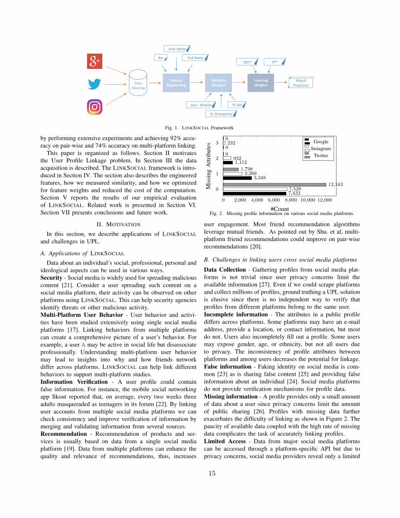
We propose a scalable, efficient, accurate framework calledLINKSOCIAL, for linking user profiles on multiple platforms.The framework is depicted in Figure 1. To the left of thefigure, LINKSOCIAL collects profiles from Google+, Twitter,and Instagram. The data is cleaned and features of the dataare extracted. Next, the similarity is measured in variousways, depending on the feature. Preliminary matches are thenrefined, and a final match prediction is made. Our empiricalevaluation shows the efficacy of LINKSOCIAL.

This paper makes three major contributions.1) We describe how to engineer relevant features for linkinguser profiles across multiple social media platforms. We showthat highly accurate linkage can be achieved by using relativelyfew public features.2) We show how to decrease the high computation cost of UPLby using clustering. Our intuition is that if we can reduce thenumber of linkage attempts, then the cost will decrease, sowe focus on pruning low similarity linkages. Given a user’sprofile from one social media platform, to find similar profilesfrom other platforms, we cluster candidate profiles usingsimilarity based on bi-grams of the username and name. Ourexperiments show that optimization preserve accuracy whilereducing computation by 90%. The cost reduction claimeddoes not include pre-computing cost of Jaccard similarity.3) We empirically evaluate the effectiveness of our framework

14

Data Cleaning

Feature Engineering

Bio

User Name

Full Name

SimilarityMeasure

LearningWeights

MatchPrediction

Jaro - Winkler TF-IDF

KL-Divergence

SGD* RF*

Fig. 1. LINKSOCIAL Framework

by performing extensive experiments and achieving 92% accu-racy on pair-wise and 74% accuracy on multi-platform linking.

This paper is organized as follows. Section II motivatesthe User Profile Linkage problem. In Section III the dataacquisition is described. The LINKSOCIAL framework is intro-duced in Section IV. The section also describes the engineeredfeatures, how we measured similarity, and how we optimizedfor feature weights and reduced the cost of the computation.Section V reports the results of our empirical evaluationof LINKSOCIAL. Related work is presented in Section VI.Section VII presents conclusions and future work.

II. MOTIVATION

In this section, we describe applications of LINKSOCIALand challenges in UPL.

A. Applications of LINKSOCIAL

Data about an individual’s social, professional, personal andideological aspects can be used in various ways.Security - Social media is widely used for spreading maliciouscontent [21]. Consider a user spreading such content on asocial media platform, their activity can be observed on otherplatforms using LINKSOCIAL. This can help security agenciesidentify threats or other malicious activity.Multi-Platform User Behavior - User behavior and activi-ties have been studied extensively using single social mediaplatforms [17]. Linking behaviors from multiple platformscan create a comprehensive picture of a user’s behavior. Forexample, a user A may be active in social life but disassociateprofessionally. Understanding multi-platform user behaviormay lead to insights into why and how friends networkdiffer across platforms. LINKSOCIAL can help link differentbehaviors to support multi-platform studies.Information Verification - A user profile could containfalse information. For instance, the mobile social networkingapp Skout reported that, on average, every two weeks threeadults masqueraded as teenagers in its forum [22]. By linkinguser accounts from multiple social media platforms we cancheck consistency and improve verification of information bymerging and validating information from several sources.Recommendation - Recommendation of products and ser-vices is usually based on data from a single social mediaplatform [19]. Data from multiple platforms can enhance thequality and relevance of recommendations, thus, increases

0 2,000 4,000 6,000 8,000 10,000 12,000

0

1

2

3

7,432

3,348

1,112

0

7,528

2,266

932

232

12,163

1,798

0

0

#CountM

issi

ngA

ttrib

utes

GoogleInstagram

Twitter

Fig. 2. Missing profile information on various social media platforms.

user engagement. Most friend recommendation algorithmsleverage mutual friends. As pointed out by Shu. et al, multi-platform friend recommendations could improve on pair-wiserecommendations [20].

B. Challenges in linking users cross social media platforms

Data Collection - Gathering profiles from social media plat-forms is not trivial since user privacy concerns limit theavailable information [27]. Even if we could scrape platformsand collect millions of profiles, ground truthing a UPL solutionis elusive since there is no independent way to verify thatprofiles from different platforms belong to the same user.Incomplete information - The attributes in a public profilediffers across platforms. Some platforms may have an e-mailaddress, provide a location, or contact information, but mostdo not. Users also incompletely fill out a profile. Some usersmay expose gender, age, or ethnicity, but not all users dueto privacy. The inconsistency of profile attributes betweenplatforms and among users decreases the potential for linkage.False information - Faking identity on social media is com-mon [23] as is sharing false content [25] and providing falseinformation about an individual [24]. Social media platformsdo not provide verification mechanisms for profile data.Missing information - A profile provides only a small amountof data about a user since privacy concerns limit the amountof public sharing [26]. Profiles with missing data furtherexacerbates the difficulty of linking as shown in Figure 2. Thepaucity of available data coupled with the high rate of missingdata complicates the task of accurately linking profiles.Limited Access - Data from major social media platformscan be accessed through a platform-specific API but due toprivacy concerns, social media providers reveal only a limited

15

amount of data. Even after collecting data, we might lackenough common features to link profiles.

III. PROBLEM DEFINITION

This section gives the problem statement, and discusses datacollection and pre-processing.

A. Problem Statement.

Let P ki be the ith public profile on social media platform

k. Let I be an identify function that maps a P ki to the identity

of the user who created the profile. For linking profiles fromn social media platforms, we use the following objectivefunction.

Φn(P 1i , . . . , P

nk ) =

{1 if I(P 1

i ) = . . . = I(Pnk )

0 otherwise(1)

Our goal is to build and learn functions Φ2(.) and Φ3(.) forlinking pair-wise and three-platform profiles. We assume thatin our dataset, every user has exactly one profile in each socialmedia platform.

B. Dataset Collection

For testing a UPL solution, we need ground truth data.While social media platforms have APIs to access user data,there is no platform to help us link a profile to an individual.However, there are ways that we could build a set of groundtruths. For instance, we could crowd-source the ground-truthing (viz. Amazon Mechanical Turks) or use surveys [22],but these methods are prone to getting unreliable data. Instead,we used a novel resource, the website about.me, which is asite that requires users to input links to profiles on other socialmedia platforms . When creating a profile on the site, a userwill provide links to their other social media profiles.

We used a dataset of 15,298 usernames from six social me-dia platforms: Google+, Instagram, Tumblr, Twitter, Youtube,and Flickr [12]. We narrowed the dataset to Instagram, Twitter,and Google+ for our study since they make the username,name, bio, and profile image are publicly available.

Next, we built a crawler to collect profiles from the threeplatforms. Table II displays information about our collecteddata. We gathered data on 7,729 users from all three platforms,6,039 users have data available on a pair of platforms and1,530 have data available only from one platform. Missingprofiles could be because of users deactivating their accounts.

C. Dataset Analysis

We analyzed the collected profiles to determine how muchinformation was missing. Figure 2 shows the count of missingprofile attributes for each platform. In Google, Twitter, andInstagram there were 28%, 13% and 21% of user profileswith at least one missing attributes, respectively. 9% and 8%of Google and Instagram profiles had at least two missingattributes. There were 87%, 62%, and 69% of profiles onTwitter, Google, and Instagram, respectively, without miss-ing information. Three attributes were missing from 2% ofInstagram profiles, making it impossible to match them. Theattributes that were presented have some variance. On average,

TABLE INUMBER OF PROFILES OBTAINED PER SOCIAL MEDIA PLATFORM.

Social Media Profile Count

Instagram 10,958Twitter 13,961

Google+ 11,892TABLE II

NUMBER OF USERS WITH PROFILES ON PAIR-WISE ANDMULTI-PLATFORMS

Social Media Profile CountInstagram - Google+ 614Twitter - Instagram 2451Google+ - Twitter 2974

Google+ - Instagram - Twitter 7729aThere were 1530 users with only one profile.

bios on Google+ were longer than Instagram and Twitter;164 characters on Google+ compared to 70 and 96 for Insta-gram and Twitter. However, the username attribute has littlevariance, it was 11-13 characters on average across all threeplatforms.

IV. THE LINKSOCIAL FRAMEWORK

This section describes LINKSOCIAL, discusses computationcost, and shows how to reduce the cost using clustering.A. Feature Engineering

LINKSOCIAL uses the basic features in a profile as well asthe following engineered features.

Username and Name bi-grams - The username is animportant feature for profile linkage since people tend to usethe same username across social media platforms. When anew name is used, parts of the name is often re-used. Forexample, John_snow, johnsno, and snow_john couldbelong to the same person. String similarity metrics such asJaro-Winkler, longest common subsequence, or Levenshteindistance, tend to perform poorly on name transpositions [34].To better align names, we engineer the bi-grams of usernamesas a feature. We also merge the bi-grams of usernames withthe bi-grams of names as a feature since people also like totranspose their surname and first name in for a username. Weengineer the following feature sets.

• bi-gram of username. (uu)• bi-gram of name. (un)• merging above two features. (ub)

These three feature sets capture a range of different ways tocreate a username.

Character Distribution - User’s like to create usernamesusing substrings of their name or other personal information(a pet’s name or a significant date). To handle scenarios wherebi-grams could not capture the similarity, we use the characterdistribution of usernames and names as features. To measuredistribution similarity we use Kullback-Leibler divergence asdefined below,

KLdivergence(P ||Q) =n∑

i=1

P (i) · logP (i)

Q(i)(2)

where P and Q are given probability distributions. We engi-neered the following features sets using character distributionsimilarity.

16

• username. (uu sim)• name. (un sim)• username + name. (ub sim)We perform experiments on real data and have not consid-

ered scenarios where username and name have no relationship.Profile Picture Similarity - Users often use the same

profile picture in multiple platforms. To capture similaritybetween profile images, we use OpenFace [14], an open sourceimage similarity framework. Openface crops images to extractface and uses deep learning to represent the face on a 128-dimensional unit hypersphere. We use `2 norm to calculatedistance between vectors of two profile images.

B. Similarity Measures

LINKSOCIAL uses two similarity measures.Jaro-Winkler Distance - Jaro-Winkler is metric for string

matching and is commonly used when matching names inUPL [11]. Studies show that the metric performs well formatching string data [15]. Jaro accounts for insertions, dele-tions, and transpositions while Winkler improves Jaro basedon the idea that fewer errors occur early in a name.

TF-IDF and Cosine Similarity - LINKSOCIAL uses adifferent similarity measure for matching profile bios sincebios are longer than names. TF-IDF and cosine similarity arewidely used for measuring the similarity of documents.

C. Matching Profiles

LINKSOCIAL matches profiles using the basic and en-gineered features of a profile. We transform the matchingproblem into a multivariate binary classification problem andoptimize it using Stochastic Gradient Descent (SGD). It isdefined as follows:

h(x) = w0 +w1 · x1 +w2 · x2 +w3 · x3 + ...+wm · xm (3)

In the equation, x1, x2, ..., xm represents the similarity scoreof features between two profiles and w1, w2, ..., wm representstheir respective weights or coefficient. We use Mean SquaredError (MSE), as our loss function. Considering the predictedvalues as hw(x)(i) where i ∈ 1, 2, ..., n and y(i) as a givenvalue (either a match (1) or no match (0)), we define MSEor cost function fcost(W ) as follows:

MSE = fcost(W ) =1

M

m∑

i=1

(y(i) − hw(x)(i)

)2(4)

LINKSOCIAL uses SGD to optimize the cost function.Partial derivatives of Equation 4 w.r.t to w1 & w2 are definedas follows:

5w1f

′cost(w1) =

1

M

m∑

i=1

−2x1(y(i) − hw(x)(i)

)

5w2f′cost(w2) =

1

M

m∑

i=1

−2x2(y(i) − hw(x)(i)

)

and similarly for other weights.

Derivatives are followed by updating of the weights. Forexample, w1 & w2 as shown below:

w1 = w1 − η5w1 f′cost(w1)

w2 = w2 − η5w2f

′cost(w2)

In the above equation, η is the learning rate, a value thattypically ranges between 0.0001 - 0.005. During experiments,we also add elastic net regularization for training.

The derivatives and weights are recursively calculated untilthe equation converges and yields an optimized weight foreach attribute based on a training set. To find a match of agiven profile we use Equation 5 where we find the profilewith maximum score on the given attributes and weights.In Equation 5, WT is a weight vector calculated using theoptimization of Equation 4 and Xu is a vector of attributes.P ki is a profile from social media platform k, while U j is a

set of all profiles from platform j.

Match(P ki , U

j) = max(WT ·Xu), ∀u ∈ U j (5)

Given profile P ki , Match() outputs the most similar profile

from platform j.

D. Computation Reduction Using Clustering

UPL can be computationally expensive. Given our datasetwith 7,729 user profiles, if we are linking pairs of profiles fromonly two of the platforms, then the number of comparisons willbe 7, 729 ∗ 7, 728 = 59, 729, 712. Assuming we can perform1,000 comparisons per second (which is a very high ballpark),it will require 17 hours to perform UPL. Matching of millionsof users across multiple platforms will be infeasible (withoutthe dedication of massive computing power).

To tackle this problem, we introduce candidate profileclustering. We can reduce the number of comparisons bypruning low potential comparisons, that is, by avoiding thework of matching profiles that are dissimilar. In our dataset,45% of the Instagram and Twitter profiles have the sameusername and name. By clustering on the bi-gram features forusername and name we can prune comparisons from profiles indifferent clusters. We have observed in previous studies [35],Jaccard similarity relativly performs well for finding similaritybetween bi-grams/n-grams and is also computationally notexpensive. We rank profiles based on Jaccard similarity andwe choose the top 10% of the candidate profiles with thehighest score in the cluster. Algorithm 1 gives our approachfor building clusters. Our clustering approach is conceptuallysimilar to kNN clustering where distance is defined by Jaccardsimilarity j sim and k is 1.

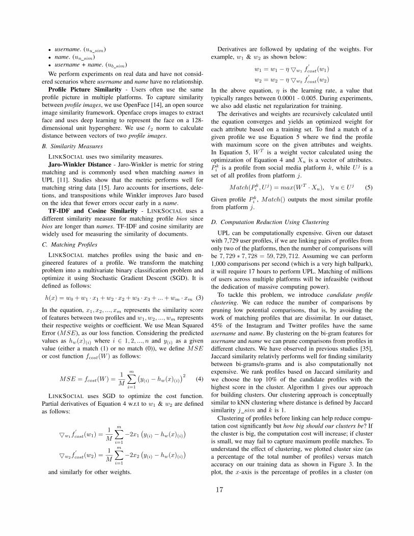
Clustering of profiles before linking can help reduce compu-tation cost significantly but how big should our clusters be? Ifthe cluster is big, the computation cost will increase; if clusteris small, we may fail to capture maximum profile matches. Tounderstand the effect of clustering, we plotted cluster size (asa percentage of the total number of profiles) versus matchaccuracy on our training data as shown in Figure 3. In theplot, the x-axis is the percentage of profiles in a cluster (on

17

1 5 10 15 20 25 30 35 40 45 5075

80

85

90

95

100

.

Cluster Size (%)

Acc

urac

y(%

)Accuracy

Fig. 3. Comparison of Cluster size to Accuracy on train data.

average). The y-axis shows the maximum accuracy we canachieve since the matching profile has to be in the cluster.We observed that clusters roughly 10% of the size of the datareduces 90% of computation cost while preserving ∼90% ofthe potential matches.

Algorithm 1 Computing candidate profiles for a given user uInput: u, U . U is set of all users from a different social media

than u.1: procedure FIND CANDIDATE PROFILE(u,U , n) . n is number

of profile to find in cluster.2: ubg ← uu + un

3: for each p ∈ U do . p is single user profile4: pbg ← pu + pn5: j sim← Jaccard similarity(ubg, pbg)6: Score[p]← j sim . Insert in dictionary7: end for8: Candidate Profiles = get top n(n, Score)9: return Candidate Profiles . Returns n candidate profile

similar to u10: end procedure11: procedure JACCARD SIMILARITY(ubg, pbg)12: Intersection = |ubg ∩ pbg| . Number of common

elements.13: Union = |ubg ∪ pbg| . Number of unique elements.

14: Jaccard Similarity =Intersection

Union15: return Jaccard Similarity16: end procedure17: procedure GET TOP N(n, Score)18: Score← Sort(Score) . Sort Score w.r.t value19: top key = get key(Score, n) . returns top n key from

sorted Score20: for each key ∈ top key do21: top n← Score[key]22: end for23: return top n . return top n candidate profiles24: end procedure

V. EXPERIMENTS

This section reports an experimental evaluation of LINKSO-CIAL. We establish a baseline for UPL and verify thatLINKSOCIAL can learn Equation 5 and achieve high matchingaccuracy. We use several variations of calculating weights andcompare them with the baseline to determine the impact ofthe weight calculations. Specifically, we use Random Forest(RF) and Stochastic Gradient Descent (SGD) for calculatingweights. We also performed feature analysis to understandwhich features are important.

TABLE IIICOMPARISON WITH PREVIOUS RESEARCH

Lin

kage

Authors Reduce Scalable

et. al Features Dataset Scalable Cost Across

Public Platform

Pair-

Wis

e

P. Jain[28] Private 5 5 5 5

A. Mal[8] Public 5 5

R. Zafa[22] Public 5 5 5 5

Y. Li[31] Private 5 5 5 5

LINKSOCIAL Public

Acr

oss X. Mu[32] Private 5 5 5

S. Liu[6] Private 5 5 5

LINKSOCIAL Public

A. Experimental Setup

We used the data described in Section III-B. We chose a60-40 split in the data for training and testing.

Baseline - We built a baseline using Jaro-Winkler and TF-IDF as discussed in Section IV-B. We use Jaro-Winkler toanalyze username and name similarity, and TF-IDF and cosinesimilarity for profile bios. To find the match of a user profile,we select a profile with the highest score from Equation 6where the value of the W vector is 1, considering each featureis equally important and X represents the feature vector.

f(W ) = WT ·Xu (6)

Calculating Weights - To calculate weights for pair-wiselinking, we generated all the features discussed in Sec-tion IV-A for each pair, which gives us data for correctmatches. To generate data for mismatches, we randomly chosepairs equal to the number of correct matches and collectedtheir feature scores.

We used normalized variable importance score from RF andalso SGD optimization algorithm as explained in Section IV-Cfor weights calculation. RF was trained using 10-Fold CrossValidation, it was tuned using grid search, and the squareroot of the number of features was selected as the numberof variables to be randomly sampled as candidates at eachsplit. SGD was also performed on the same dataset to calculateweights with a learning rate η of 0.001, with 1,000 iterations.

Computing Candidate Profile - To compute candidatepairs, we follow the approach described in Algorithm 1. Intraining, we pre-compute each profile’s potential matches. Togenerate a feature vector we score based on clusters. To makesure we have both positive and negative label samples of equalsize, we randomly sample negative label data of the same sizeas the positive label set and generated samples are used tolearn the weight vector.

Multi-Platform Profile Linking - We link users acrossthree platforms similar to how we perform pair-wise linking.Due to the very high computation cost, we were unable torun experiments for linking without first clustering candidateprofiles. We performed experiments by adding and removingengineered features. To find a similar profile, we choose aprofile in one social media platform and tried to find thematching profiles in the other two platforms. We performed

18

TABLE IVLINKSOCIAL PERFORMANCE ON PAIR-WISE UPL

Social Media Pairs (Accuracy %)Experiments G+≡I T≡ I G+≡Tbaseline 55.36% 77.86% 56.86%

Prediction without engineered features and clustering.with RF 77.53% 82.08% 77.14%

with SGD 76.61% 82.21% 66.24%Prediction with clustering, no engineered features.

with CP & RF 82.62% 83.33% 81.40%with CP & SGD 82.47% 83.32% 81.19%

Prediction with engineered features, no clustering.with RF 86.54% 91.17% 84.56%

with SGD 86.63% 91.68% 84.58%Prediction with engineered features and clustering.

with CP & RF 84.85% 87.92% 83.20%with CP & SGD 84.91% 88.29% 83.23%

this experiment for each platform. During training, we choosea platform and compute its respective candidate profiles fromother platforms by building feature vector between candidateprofiles and the given profile. We then perform SGD and RF tocalculate weights for each feature and we used the calculatedweights to find similar profiles.

Previous research comparison - Table III compares ourapproach to previous approaches in terms of feature selection,data availability and scalability. Previous approaches haveused different types of features in their algorithms. A publicfeature is publicly available information (e.g., bio, profileimage, name, user name). Private data such as locationdata is proprietary limiting the feasibility of approaches thatrely on such information since they need cooperation frombusinesses that compete against each other. Making a publiclyavailable benchmark dataset is an important aspect for futurework and comparison of approaches. Previous researchershave not shared their data (because of privacy concerns anddata sources), where as in our approach we have collectedall data as public information and have made it availablefor future research/comparison. As discussed earlier, UPL isa computationally expensive process and scalability of anapproach depends on using methods to reduce computationcost to make the solution practical in a real-life scenario. Also,designing an algorithm to scale for new/several platforms isvery important aspect. Only a few approaches in past haveused computation cost reduction and are designed to scale fornew social media platforms.

Previous work accuracy Table VI reports accuracies in asampling of previous research in both pair-wise and multi-platform linkage. The accuracy is reported “as is” from thepapers, experimental setups and measurements differ acrosspapers, for instance previous work with better accuracy forpair linkage used user generated content data (gaining accessto such data is difficult) but in our approach we use onlypublicly available profile data We observe that LINKSOCIALis among the leaders in pair-wise UPL and the best at multi-platform UPL.

TABLE VLINKSOCIAL PERFORMANCE ON MULTI-PLATFORM UPL

Cross PlatformExperiments T→(G+, I) G+→(T, I) I→(G+,T)

CP & RF 71.56% 72.50% 73.70%CP & SGD 72.95% 72.86% 74.18%

*RF−Random Forest, SGD−Stochastic Gradient Descent, CP−CandidateProfiles using Clustering, T−Twitter, G+−Google+, I−Instagram

TABLE VIREPORTED ACCURACY FROM FEW PREVIOUS WORK.

Linkage Authors AccuracyPair-Wise P. Jain et al. [28] 39.0%

Social A. Malhotra et. al. [8] 64.0%Platform R. Zafarani et. al. [22] 93.8%Linkage Y. Li et. al. [31] 89.5%

Our Approach 91.68%Across X. Mu et. al. [32] 44.00%

Multiple S. Liu et. al. [6] (reported by [32]) 42.00%Platform Our Approach 74.18%

B. Evaluation Metrics

In previous studies, accuracy has been used as a reliableevaluation metric for UPL [28]. Given two profiles fromdifferent platforms, the accuracy of such matching can bemeasured as follows. First, assume the following are known.

• Total number of correct prediction (P): Number of correctpositive prediction by LINKSOCIAL.

• Total number of positive sample (N): Number of positivelinked profiles in the dataset.

Then the accuracy can be computed as follows.

Accuracy(%) =|P ||N | · 100 (7)

C. Results

We performed several experiments on pair-wise linking andthe results are shown in Table IV and Table V. Specifically,we measured the accuracy of LINKSOCIAL on all possiblepairs in our dataset namely, Google+ - Twitter, Google+- Instagram, and Twitter - Instagram. We also performedexperiments with features and weights calculated using RFand SGD. As shown in Table [IV], we started with buildinga baseline for each pair. We achieved 55%, 78%, 57% forGoogle+ - Instagram, Twitter - Instagram and Google+ -Twitter respectively. We then performed experiments withoutusing engineered features and clustering. We observed thatRF produced more accurate matches than SGD. Next, weadded candidate pairs but sill no engineered features. In thiscase, both RF and SGD performed equally well. We thenadded engineered features and perform experiments withoutclustering. We observed that SGD outperformed RF. Finally,we used both engineered features and clustering. SGD againperformed better than RF. Overall, weights calculated usingSGD proved to be more accurate than RF though in some casesthe difference was marginal. In the final stage, we observedreduction of accuracy by adding clustering. This is due tothe inconsistent username and name used by a user, sinceclustering uses username and name (in our dataset, out of all

19

0.3

0.4

0.5

0.00 0.25 0.50 0.75 1.00User Name Bigram Similarity Score

yhat

0.2

0.3

0.4

0.5

0.00 0.25 0.50 0.75 1.00Merged Bigram Similarity Score

yhat

0.48

0.50

0.52

0.00 0.25 0.50 0.75Merged Distribution Similarity Score

yhat

0.30

0.35

0.40

0.45

0.50

0.00 0.25 0.50 0.75 1.00Full Name Bigram Similarity Score

yhat

0.30

0.35

0.40

0.45

0.50

0.00 0.25 0.50 0.75 1.00User Name Similarity Score

yhat

0.35

0.40

0.45

0.50

0.00 0.25 0.50 0.75 1.00Full Name Similarity Score

yhat

0.48

0.49

0.50

0.0 0.2 0.4 0.6Full Name Distribution Similarity Score

yhat

0.4950

0.4975

0.5000

0.5025

0.5050

0.0 0.1 0.2 0.3 0.4 0.5User Name Distribution Similarity Score

yhat

Fig. 4. Partial Dependence Plots for individual features.

0.0

0.1

0.2

0.3

0.4

0.5

0.0 0.2 0.4 0.6 0.8Merged Distribution Similarity Score

Use

r N

am

e D

istr

ibu

tion

Sim

ilari

ty S

core

0.48

0.50

0.52

0.54

Partialdependence

0.00

0.25

0.50

0.75

1.00

0.00 0.25 0.50 0.75 1.00User Name Similarity Score

Fu

ll N

am

e S

imila

rity

Sco

re

0.3

0.4

0.5

Partialdependence

Fig. 5. Partial Dependence Plots for selected pairs of features.

pairs, maximum of 45% users have the same username and22.2% of users with the same name), but slight decrease inaccuracy could be traded for speed.

We performed several experiments on multi-platform link-ing and the results are shown in Table V. We observedthat, feature weights computation using SGD again outper-formed RF. We achieved an accuracy of 73%, 73%, 74%for Twitter→(Google+, Instagram), Google+→(Twitter, Insta-gram), and Instagram→(Twitter, Google+) respectively. Over-all, in our experiments on multi-platform linkage, SGD provedto more accurate.

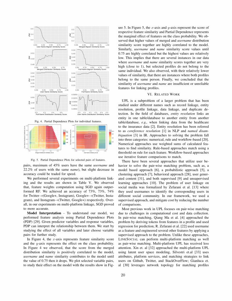
Model Interpretation - To understand our model, weperformed feature analysis using Partial Dependence Plots(PDP) [29]. Given predictor variables and response variables,PDP can interpret the relationship between them. We start bystudying the effect of all variables and later choose variablepairs for further study.

In Figure 4, the x-axis represents feature similarity scoreand the y-axis represents the effect on the class probability.In Figure 4 we observed, that the score from the mergeddistribution similarity is positively correlated to the model,username and name similarity contributes to the model untilthe value of 0.75 then it drops. We plot selected variable pairs,to study their effect on the model with the results show in Fig-

ure 5. In Figure 5, the x-axis and y-axis represent the score ofrespective feature similarity and Partial Dependence representsthe marginal effect of features on the class probability. We ob-served that higher values of merged and username distributionsimilarity score together are highly correlated to the model.Similarly, username and name similarity score values until0.75 are highly correlated but the highest values are relativelylow. This implies that there are several instances in our datawhere username and name similarity scores together are veryhigh (close to 1), but selected profiles do not belong to thesame individual. We also observed, with their relatively lowervalues of similarity, that there are instances where both profilesbelong to the same person. Finally, we concluded that thesimilarity of username and name are insufficient or unreliablefeatures for linking profiles.

VI. RELATED WORK

UPL is a subproblem of a larger problem that has beenstudied under different names such as record linkage, entityresolution, profile linkage, data linkage, and duplicate de-tection. In the field of databases, entity resolution links anentity in one table/database to another entity from anothertable/database, e.g., when linking data from the healthcareto the insurance data [2]. Entity resolution has been referredto as coreference resolution [1] in NLP and named disam-biguation [3] in IR. Approaches to solving the problem fallinto three categories: numerical, rule and workflow-based [20].Numerical approaches use weighted sums of calculated fea-tures to find similarity. Rule-based approaches match using athreshold on rule for each feature. Workflow-based approachesuse iterative feature comparisons to match.

There have been several approaches that utilize user be-havior to solve the pair-wise matching problem, such as, amodel based approach [6], a probabilistic approach [5], aclustering approach [7], behavioral approach [28], user gener-ated content [31], and both supervised [9] and unsupervisedlearning approaches [10]. The problem of user linkage onsocial media was formalized by Zefarani et al. [13] wherethey used usernames to identify the corresponding users indifferent social community. In our framework, we used asupervised approach, and mitigate cost by reducing the numberof comparisons.

Most previous work in UPL focuses on pair-wise matchingdue to challenges in computational cost and data collection.In pair-wise matching, Qiang Ma et al. [4] approached theproblem by deriving tokens from features in a profile and usedregression for prediction; R. Zefarani et al. [22] used usernameas a feature and engineered several other features by applying asupervised approach to the problem. Unlike these approaches,LINKSOCIAL can perform multi-platform matching as wellas pair-wise matching. Multi-platform UPL has received lessattention. Xin et. al [32] approached the multi-platform UPLusing latent user space modeling, Silvestri et.al [33] usesattributes, platform services, and matching strategies to linkusers on Github, Twitter, and StackOverFlow; Gianluca et.al [30] leverages network topology for matching profiles

20

across n social media. Liu et. al. [6] uses heterogeneous userbehavior (user attributes, content, behavior, network topology)for multi-platform UPL but gaining access to such data is nota trivial task.

VII. CONCLUSION

In this paper, we investigate the problem of User ProfileLinkage (UPL) across social media platforms. Multi-platformlinkage can provide a richer, more complete foundation forunderstanding a user’s on-line life and can help improveseveral research studies currently performed only on singlesocial media platform. UPL has many potential applicationsbut is challenging due to the limited, incomplete, and po-tentially false data on which to link. We proposed a largescale, efficient and scalable solution to UPL which we callLINKSOCIAL. LINKSOCIAL links profiles based on a fewcore attributes in a public profile: username, name, bio andprofile image. Our framework consists of (1) feature extraction,(2) computing feature weights, and (3) linking pair-wise andmulti-platform user profiles. We performed extensive experi-ments on LINKSOCIAL using data collected from three popularsocial media platforms: Google+, Instagram and Twitter. Weobserved that username and name alone are an insufficientset of features for achieving highly accurate UPL. UPL iscomputationally costly, but we showed how to use clustering toreduce the cost without sacrificing accuracy. Candidate profileclustering is based on pruning dissimilar profile comparisons.It reduced 90% of the comparisons which significantly helpedin scaling our framework. We evaluate our framework on bothpair-wise and multi-platform profile linkage with accuracy91.68% on pair-wise and 74.18% on multi-platform linkage.

Data about a user from multiple social media platformshas many applications. In future, we plan to (1) extend ourwork to study a user’s behavior across platforms, whichto our knowledge has not yet been studied, (2) add morefeatures to LINKSOCIAL using heterogeneous data, e.g., usercontent similarity (text, videos, images), network similarity,and patterns across social media platforms, and (3) evaluateLINKSOCIAL on more (up to six) social media platforms.

REFERENCES

[1] J. Cai, M. Strube, “End-to-End Coreference Resolution via HypergraphPartitioning,” COLING, 2010.

[2] S. E. Whang, D. Marmaros, H. Garcia-Molina, “Pay-As-You-Go EntityResolution,” IEEE Transactions on Knowledge and Data Engineering,2013.

[3] Y. Qian, Y. Hu, J. Cui, Q. Zheng, Z. Nie, “Combining machine learningand human judgment in author disambiguation,” CIKM, 2011.

[4] Q. Ma, H. H. Song, S. Muthukrishnan, A. Nucci, “Joining user profilesacross online social networks: From the perspective of an adversary,”IEEE/ACM ASONAM, 2016.

[5] H. Zhang, M. Kan, Y. Liu, S. Ma, “Online Social Network ProfileLinkage,” AIRS, 2014.

[6] S. Liu, S. Wang, F. Zhu, J. Zhang, R. Krishnan, “HYDRA: large-scalesocial identity linkage via heterogeneous behavior modeling,” SIGMODConference, 2014.

[7] W. W.Cohen, J. Richman, “Learning to match and cluster large high-dimensional data sets for data integration,” KDD, 2002.

[8] A. Malhotra, L. C.Totti, W. Meira Jr., P. Kumaraguru, V. A. F. Almeida,“Studying User Footprints in Different Online Social Networks,” 2012IEEE/ACM International Conference on Advances in Social NetworksAnalysis and Mining, 2012.

[9] A. Nunes, P. Calado, B. Martins, “Resolving user identities over socialnetworks through supervised learning and rich similarity features,” SAC,2012.

[10] J. Liu, F. Zhang, X. Song, Y. Song, C. Lin, H. Hon, “What’s in a name?:an unsupervised approach to link users across communities,” WSDM,2013.

[11] W. E. Winkler, “Overview of record linkage and current researchdirections,” BUREAU OF THE CENSUS, 2006.

[12] B. Lim, D. Lu, T. Chen, M. Kan, “# mytweet via instagram: Exploringuser behaviour across multiple social networks,” Advances in Social Net-works Analysis and Mining (ASONAM), 2015 IEEE/ACM InternationalConference on, 2015.

[13] R. Zafarani, H. Liu, “Connecting Corresponding Identities across Com-munities.,” ICWSM, 2009.

[14] T. Baltruvsaitis, P. Robinson, L. Morency, “Openface: an open sourcefacial behavior analysis toolkit,” Applications of Computer Vision(WACV), 2016 IEEE Winter Conference on, 2016.

[15] W. Cohen, P. Ravikumar, S. Fienberg, “A comparison of string metricsfor matching names and records,” Kdd workshop on data cleaning andobject consolidation, 2003.

[16] L. Manikonda, V. V. Meduri, S. Kambhampati, “Tweeting the Mind andInstagramming the Heart: Exploring Differentiated Content Sharing onSocial Media,” ICWSM, 2016.

[17] F. Benevenuto, T. Rodrigues, M. Cha, V. A. F. Almeida, “Character-izing user behavior in online social networks,” Internet MeasurementConference, 2009.

[18] P. Bhattacharya, M. BilalZafar, N. Ganguly, S. Ghosh, K. P. Gummadi,“Inferring user interests in the Twitter social network,” RecSys, 2014.

[19] M. Jamali, M. Ester, “A matrix factorization technique with trustpropagation for recommendation in social networks,” RecSys, 2010.

[20] K. Shu, S. Wang, J. Tang, R. Zafarani, H. Liu, “User Identity Linkageacross Online Social Networks: A Review,” SIGKDD, 2016.

[21] J. Klausen, “Tweeting the Jihad: Social media networks of Westernforeign fighters in Syria and Iraq,” Studies in Conflict & Terrorism,2015.

[22] R. Zafarani, H. Liu, “Connecting users across social media sites: abehavioral-modeling approach,” KDD, 2013.

[23] S. C. Herring, S. Kapidzic, “Teens, Gender, and Self-Presentation inSocial Media,” KDD, 2014.

[24] G. S. O’Keeffe, K. Clarke-Pearson, “The impact of social media onchildren, adolescents, and families.,” Pediatrics, 2011.

[25] D. Miller, E. Costa, N. Haynes, T. McDonald, R. Nicolescu, J. Sinanan,J. Spyer, S. Venkatraman, X. Wang, “How the world changed socialmedia,” UCL press, 2016.

[26] R. Gross, A. Aless, “Information revelation and privacy in online socialnetworks,” WPES, 2005.

[27] J. M. Kleinberg, “Challenges in mining social network data: processes,privacy, and paradoxes,” KDD, 2007.

[28] P. Jain, P. Kumaraguru, A. Joshi, “@I Seek ’Fb.Me’: Identifying UsersAcross Multiple Online Social Networks,” WWW, 2013.

[29] A. Goldstein, A. Kapelner, J. Bleich, E. Pitkin, “Peeking inside the blackbox: Visualizing statistical learning with plots of individual conditionalexpectation,” journal of Computational and Graphical Statistics, 2015.

[30] G. Quercini, N. Bennacer, M. Ghufran, C. NanaJipmo, “LIAISON: rec-onciLIAtion of Individuals Profiles Across SOcial Networks,” Advancesin Knowledge Discovery and Management: Volume 6, 2017.

[31] Y. Li, Z. Zhang, Y. Peng, H. Yin, Q. Xu, “Matching user accounts basedon user generated content across social networks,” Future GenerationComputer Systems, 2018.

[32] X. Mu, F. Zhu, E. Lim, J. Xiao, J. Wang, Z. Zhou, “User IdentityLinkage by Latent User Space Modelling,” Proceedings of the 22NdACM SIGKDD International Conference on Knowledge Discovery andData Mining, 2016.

[33] G. Silvestri, J. Yang, A. Bozzon, A. Tagarelli, “Linking Accountsacross Social Networks: the Case of StackOverflow, Github and Twitter,”KDWeb, 2015.

[34] P. Christen “A Comparison of Personal Name Matching: Techniques andPractical Issues,” Workshops Proceedings of the 6th IEEE ICDM, 2006.

[35] M. Krieger and D. Ahn “TweetMotif: exploratory search and topicsummarization for Twitter,” In Proc. of AAAI Conference on Weblogsand Social, 2010

21

22

CHAPTER 3

MANTIS: Multiple Type and Attribute Index Selection

using Deep Reinforcement Learning

MANTIS: Multiple Type and Attribute IndexSelection using Deep Reinforcement Learning

Vishal Sharma, Curtis Dyreson, and Nicholas Flann

Department of Computer Science, Utah State University, Utah, USA{vishal.sharma, curtis.dyreson, nick.flann}@usu.edu

Abstract. DBMS performance is dependent on many parameters, suchas index selection, cache size, physical layout, and data partitioning.Some combinations of these parameters can lead to optimal performancefor a given workload but selecting an optimal or near-optimal combina-tion is a challenging task, especially for large databases with complexworkloads. Among the hundreds of parameters, index selection is ar-guably the most important parameter for performance. We propose aself-administered framework, called the Multiple Type aNd Attribute In-dex Selector (MANTIS), that automatically selects near optimal indexes.The framework advances the state-of-the-art index selection by consider-ing both multi-attribute and multiple types of indexes within a boundedstorage size constraint, a combination not previously addressed. MAN-TIS combines supervised and reinforcement learning, a Deep Neural Net-work recommends the type of index for a given workload while a DeepQ-Learning network recommends the multi-attribute aspect. MANTISis sensitive to storage cost constraints and incorporates noisy rewards inits reward function for better performance. Our experimental evaluationshows that MANTIS outperforms the current state-of-art methods by anaverage of 9.53% QphH@size.

1 Introduction

The performance of a database application is critical to ensuring that the appli-cation meets the needs of customers. An application’s performance often dependson the speed at which workloads, i.e., a sequences of data retrieval and updateoperations, are evaluated. A database can be tuned to improve performance, e.g.,by creating an index or increasing the size of the buffer. Figure 1(b) shows theimpact of just two configuration parameters, Memory Size and Buffer Size, onworkload performance. We observe that choosing an optimal combination canenhance performance significantly. Currently a database administrator (DBA)manually tunes performance by monitoring performance over time and adjustingparameters as needed. But the growing number of configuration parameters, asshown in Figure 1(a), has increased the complexity of manually tuning perfor-mance.

For many queries, e.g., range and lookup queries, a database index signif-icantly reduces query time. An index can be created on a single column or

23

2 V. Sharma et al.

2005 2010 2015 2020Years

100150200250300

Num

ber o

f par

amete

rs

Growth in the number of parameters of Postgres (2000-2020)

Postgres

(a)Buffer Size (kB)1600 2400 3200 4000

Memory size (kB)1600240032004000

Total

Tim

e (se

c)

24.525.025.526.026.527.027.5

Parameters effect on workload performance

(b)

Fig. 1. Figure (a) shows number of parameters in Postgres (2000-2020). Figure (b)shows effect on a workload performance using different parameter settings

several columns of a database table. There are also different types of indexes,for instance, Postgres has six index types: B-tree, Hash, GiST, SP-GiST, GINand BRIN. One possible solution is to simply create all possible indexes for adatabase, but this approach is infeasible due to large number of potential in-dexes, e.g., for a single kind of index (B-tree) on a table with N columns, thereare 2N −1 potential (multi-column) indexes. There are two other reasons why itis important to limit the number of indexes in a database. First, there are spaceconsiderations. An index occupies space in secondary storage that increases the(stored) size of a database. Second, indexes slow down data modification sincemodifications need to update both the data and the index. Creating too manyindexes can decrease the throughput and latency of a database. Hence the setof indexes created for a database should be parsimonious, while too few indexesmay slow query evaluation, too many may increase space cost and slow downdata modification.

The index recommendation problem can be defined as finding a set of indiceswhich minimizes the time taken to evaluate a workload and the amount of stor-age used. Finding a set of indexes which minimizes the cost is a combinatorialoptimization problem, and adding a disk size constraint makes this problem aconstrained combinatorial optimization problem. Finding an optimal solution forsuch a problem is NP-hard [19] but Reinforcement Learning (RL) [12] has beenused to find approximate solutions for large scale combinatorial optimizationproblems such as for vehicle routing [17], directed acyclic graph discovery [29],and the traveling salesman problem [14]. RL has also shown that it can learncomplex database tasks with a large search space, such as learning optimal pa-rameter configuration for a workload [22].

In this paper, we apply RL to maximize query performance by learning whichindexes would be the best to create for a given workload. There has been previousresearch on index recommendation using Reinforcement Learning [1, 2, 13, 25].However, previous research has been limited in one of three ways. First, previousresearch has focused on one type of index, B-Tree, but DBMSs typically supportseveral types,e.g., Postgres has six types. Second, most previous research has in-

24

Title Suppressed Due to Excessive Length 3

vestigated creating only single attribute indexes, but multi-attribute indexes canimprove the performance of many queries. Third, previous research has not con-sidered a constraint on storage size, that is, the approaches are non-parsimoniousand allow the creation of more indexes than needed (there is no penalty for cre-ating too many indexes). A generic framework that captures multi-attribute anddifferent types of indexes is an open research problem. We propose an end-to-end index recommendation system that we call the Multiple Type aNd AttributeIndex Selector (MANTIS). MANTIS can learn to recommend multi-attributeindexes of different types within a given size constraint.

This paper makes the following contributions.

– We formulate the Index Recommendation Problem as a Markovian DecisionProcess. We implement a disk size constraint to limit the total index size inour reward function.

– We propose an end-to-end multi-attribute and multi-index type recommen-dation framework. Our framework, MANTIS, uses Deep Neural Networksand Deep Q-Learning Networks for recommendations.

– We perform extensive experiments on MANTIS and compare results withcurrent state-of-the-art methodologies.

– We make our code and experimental setup publicly available.

This paper is organized as follows, the next section presents related work.Section 3 gives a precise formulation of the index recommendation problem whileSection 4 describes our MANTIS solution to the problem. We present the eval-uation of the performance of MANTIS in Sections 5 and 6. Section 7 presentsconclusions and future work.

2 Related work

A database can be tuned using either external or internal methods. An exter-nal tuning method uses an API to configure a DBMS while an internal methodembeds tuning algorithms in the DBMS. External tuning is widely used becauseit is generally applicable. Internal tuning needs access to a DBMSs internals,which may be proprietary or dependent on the software architecture of a partic-ular DBMS. Most of the approaches discussed here are external. Internal tuningis primarily industry-based, e.g., the Oracle9i optimizer.

In recent years, Reinforcement Learning (RL) has become a popular externaltuning method and has been used to optimize join order [15, 24, 27], in queryoptimization [7,8,16,18], to self-tune databases [11,28] and to improve data par-titioning [3, 5, 26]. For the index selection problem, Basu et al. [1] proposed atuning strategy using Reinforcement Learning. They formulate the index selec-tion problem as a Markovian Decision Process and use a state-space reductiontechnique to scale their algorithm for larger databases and workloads. Sharma etal. [22] proposed NoDBA for index selection. NoDBA stacks the workload andpotential indexes as input to the neural network and uses Deep ReinforcementLearning with a custom reward function for index recommendation. Both of the

25

4 V. Sharma et al.

above approaches consider only single attribute indexes and a single kind ofindex. They are unable to recommend multi-attribute indexes. Welborn et al.[25] introduced latent space representation for workload and action spaces. Thisrepresentation enables them to perform other tasks, e.g., workload summariza-tion and analyzing query similarity. They used a variant of DQN with duelingcalled BDQN (Branched Deep Q-Network) for learning index recommendation.Licks et al. [13] introduced SmartIX where they use Q-Learning for indexrecommendation. In their approach, they learn to build indexes over multipletables in a database. They also evaluate SmartIX using the standard metricsQphH@size, power and throughput. They use QphH@size in their reward func-tion, which makes the evaluation process slow, and in some cases, it may takeseveral days of computation, which impacts the scalability of their approach.Kllapi et al. [6] propose a linear programming-based index recommendation al-gorithm. Their approach identifies and builds indexes during idle CPU time tomaximize CPU utilization without affecting performance. Lan et al. [9] proposean index advisory approach using heuristic rules and Deep Reinforcement Learn-ing. Sadri et al. [21] utilizes Deep Reinforcement Learning to select indexes forcluster databases.

The above approaches have mostly focused on recommending B-tree indexes.By focusing on a single type of index such approaches lack the capability of uti-lizing other types of indexes like BRIN or Hash to improve query performance.There are no previous approaches for performing an end-to-end index recom-mendation for both multi-attribute and multi-type index selection, which is thefocus of this paper. Moreover, previous approaches do not support a storagespace constraint.

3 Problem Formulation

The index recommendation problem is to select a set of indexes that minimizesthe time to evaluate a workload and the amount of storage needed.

A workload W is a set of SQL queries Q1, Q2,.., Qm. An index configurationI is a set of indexes. We calculate the cost of workload evaluation on database Dusing the cost of the evaluation of each individual query given by Cost(Qj , I,D).The cost of a workload can be described as follows.

Cost(W, I,D) =

m∑

j=1

Cost(Qj , I,D)

Note that the workload cost does not weight queries differently, though we couldtrivially include such weights by replicating individual queries in a workload.The index selection problem is to find a set of indexes Ioptimal that minimizesthe total cost of workload Cost(W, I,D) and has a storage cost of at most C.

Ioptimal = minS(I∗)≤C

Cost(W, I∗, D)

In this equation S(I∗) is the total storage space cost of the set of indexes I∗.

26

Title Suppressed Due to Excessive Length 5

4 MANTIS Framework

We designed and built our framework using Deep Neural Networks (DNN) andDeep Q-Learning Networks (DQN). In order to select a suitable set of index typesfor a workload, our first research goal is index type selection. The second researchgoal is the index recommendation to pick possible (single/multiple) attributesfor the index. Our framework, research goals, and the challenges we overcomeare described in this section.

4.1 Index Type Selection

Almost all DBMSs have several types of indexes. Though the types vary acrossDBMSs, common index types include B-tree index (which includes all B-treevariants and is often the default index type), block range index (BRIN) whichis helpful in range queries, and hash index, which improves the performance ofhash joins and point queries. Spatial indexes, such as R-tree indexes, are alsocommonly available. We trained a Deep Neural Network (DNN) to choose thebest types of indexes for a given workload. The DNN models takes workload asan input and predicts potential index types.

DNN model: We convert SQL queries in a workload to a vector representa-tion using feature extraction. Specifically, we extract features describing differentquery types for B-Tree, BRIN, Hash, and Spatial.

– feature 1: Describes the count of each operator used in a query. The oper-ators we search for are [>,<,=,≤,≥]. This feature helps us identify queriessearching for equality, range, or general. In case of equality, a Hash indexwould be preferable, and for queries based on [≤,≥] a BRIN index would bepreferred over B-Tree.

– feature 2: The number of columns mentioned in a query.– feature 3: The number of conjunctions/disjunctions [‘and’,‘or’] in a query.– feature 4: To identify spatial queries we extract certain keywords from the

query [‘.geom’, ‘.location’, ‘distance’].

Using the above features, we pre-train our DNN model. We use a fully con-nected multi-layer network with three layers. The first and second layers consistof 32 neurons with relu activation, and the output layer consists of num classes(in our case 4) with sigmoid activation. The mean squared error (mse) is usedas the cost function; the number of epochs is 30 and 30% data for validation.The model is trained using adam optimizer with a learning rate of 0.001, and weuse a learning rate decay (initial rate/epochs) for the stability of the network.

4.2 Index Recommendation

Index recommendation in MANTIS uses Deep Neural Networks for function ap-proximation with the Q-Learning algorithm, also known as the Deep Q-LearningNetwork (DQN). To build the DQN we formulate the index recommendation

27

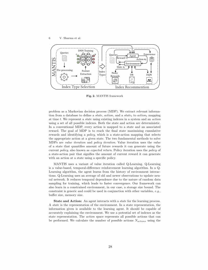
6 V. Sharma et al.

eries

DQNIndex TypesM

AN

TIS

DB

Experienceeries

FeatureExtraction

DNN Training

Index Type Selection Index Recommention

Noisy Rewards

Environment

Action Reward

State Pre-processing

Agent

Fig. 2. MANTIS framework

problem as a Markovian decision process (MDP). We extract relevant informa-tion from a database to define a state, action, and a statet to actiont mappingat time t. We represent a state using existing indexes in a system and an actionusing a set of all possible indexes. Both the state and action are deterministic.In a conventional MDP, every action is mapped to a state and an associatedreward. The goal of MDP is to reach the final state maximizing cumulativerewards and identifying a policy, which is a state-action mapping that selectsthe appropriate action at a given state. The two fundamental methods to solveMDPs are value iteration and policy iteration. Value iteration uses the valueof a state that quantifies amount of future rewards it can generate using thecurrent policy, also known as expected return. Policy iteration uses the policy ofa state-action pair that signifies the amount of current reward it can generatewith an action at a state using a specific policy.

MANTIS uses a variant of value iteration called Q-Learning. Q-Learningis a value-based, temporal-difference reinforcement learning algorithm. In a Q-Learning algorithm, the agent learns from the history of environment interac-tions. Q-Learning uses an average of old and newer observations to update neu-ral network. It reduces temporal dependence due to the nature of random datasampling for training, which leads to faster convergence. Our framework canalso learn in a constrained environment, in our case, a storage size bound. Theconstraint is generic and could be used in conjunction with other variables, e.g.,buffer size, memory size.

State and Action: An agent interacts with a state for the learning process.A state is the representation of the environment. In a state representation, theinformation given is available to the learning agent. It should be capable ofaccurately explaining the environment. We use a potential set of indexes as thestate representation. The action space represents all possible actions that canbe performed. We calculate the number of possible actions Nactions using the

28

Title Suppressed Due to Excessive Length 7

following equation:

Nactions = (2Ncolumns − 1) × len(index type)

where, index type is our DNN model predicting the possible index types to beused and (2Ncolumns − 1) is all possible combination of indexes in a table.

Reward Function: A reward function is another important component of areinforcement learning agent. We design our reward function based on workloadcost estimation. We compare the cost of the index set against the set of allpossible indexes as defined below:

rewardssize =

(1, index size < max allowed size

−1, otherwise

)

rt = max

(index cost

all index cost− 1, 0

)+ rewardssize (1)

where the numerator is the workload cost with a selected set of indexes and thedenominator is workload cost with all possible indexes. We also use a reward forthe storage size constraint.

Noisy Rewards: Inconsistent rewards can cause an agent’s performance todegrade and a learning agent will not be able to maximize rewards. Though weuse query cost estimate as a reward, previous research has shown the inefficacy ofDBMS cost estimator [10]. To minimize noise in the reward function we performan 1D convolution filter with a kernel size of five and use the filter in our rewardfunction. Given a input vector f of size k and convolution kernel g of size m a1D convolution filter can be formulated as follows.

(f ∗ g)(j) =

m∑

i=1

(g(j) · f(j − i+m/2)) /m

We experimented with several, well-known noise-reducing filters, namely Ex-ponential filter, Savitzky-Golay filter, and Kalman Filter. We found that thesefilters either over or under estimated rewards. The 1D convolution filter alsotends to underestimate the cost. However, due to its fast computation time andstreaming nature it proved to be a feasible solution. We also added a spike filterto suppress extreme values.

Agent training: The training procedure consists of Nepisodes episodes, andeach episode has Nindex steps where Nindex represents the maximum number ofindexes. During an episode, the agent performs an action based on a policy andcollects rewards for the selected action, this is known as an experience. Theseexperiences are stored in a buffer, called the Replay Buffer, for sampling andtraining. The cost of an action is calculated by its effect on the total workloadcost of retrieval using the rewards function from Equation 1. The computedrewards are adjusted using the 1D convolution filter. At the end of this stepstate, action, rewards are returned. During training we use the a configurationbatch size of 32, consisting of 100 episodes, a maximum index number of Nindex:

29

8 V. Sharma et al.

3 − 6, a priority scale of η: 0.97, a learning rate of α: 0.001, a discount factor ofβ: 0.97, and a storage bound of 10-20MB. Our complete framework is depictedin Figure 2.

5 Experimental Setup

We perform experiments on two datasets, a standard database benchmark TCP-H [23] and a real time dataset IMDB [10]. We use PostgreSQL as a choice forour database. We create an OpenGym environment for command based databaseinteraction. All experiments were performed on a computer with Intel i7 5820k,Nvidia 1080ti, 32GB of RAM running Ubuntu 18.04 OS. We use Python 3.7and libraries (powa, gym, psycopg2, sklearn, TensorFlow, Keras) to write andtrain our framework. The DNN and DQN were trained on Nvidia 1080ti (3584CUDA cores and 11GB DDR5 RAM) with CUDA and cuDNN configured forperformance enhancement.

1. TPC-H: TPC is the most well-known and most widely-used family of databasebenchmarks. TPC-H is the benchmark for decision support systems. We gen-erate a dataset of 120k tuples using TPC-H and randomly generate queriesas follows: we randomly select columns and a value from a table. We thenrandomly select an operator [>, <, =] and predicate [and, or]. By choosing be-tween one and four columns, we create four different sets of queries (1C, 2C,3C, 4C). The variety of queries assists in the validation of our framework’sefficacy. We generate 100 queries for each TPC-H experiment.Few randomly generated queries used in our experiments:

1C: SELECT COUNT(*) FROM LINEITEM WHERE L_TAX < 0.02

2C: SELECT COUNT(*) FROM LINEITEM WHERE L_ORDERKEY < 11517219

OR L_TAX < 0.02

3C: SELECT COUNT(*) FROM LINEITEM WHERE L_SUPPKEY < 18015 AND

L_PARTKEY > 114249 AND L_TAX > 0.06

4C: SELECT COUNT(*) FROM LINEITEM WHERE L_ORDERKEY = 8782339

AND L_TAX = 0.01 AND L_PARTKEY = 264524 AND L_SUPPKEY >

14028

2. IMDB: IMDB is a large database of movie-related data. There are 21 ta-bles, with a few large tables such as cast_info table, which has 36 millionrecords, and the movie_info table, which has 15 million records. It has 113computationally intensive SQL queries with multi-joins. We randomly andequally divide the queries in three stage with 37 (Stage 1), 38 (Stage 2),and 38 (Stage 3) queries. The aim of separating queries is to create morereal-time scenarios for framework validation.

5.1 Performance Metric

We measure performance using standard DBMS metrics, such as Power@size,Throughtput@Size, and QphH@Size.

30

Title Suppressed Due to Excessive Length 9

Power@Size tests the durability of the indexes chosen for inclusion anddeletion of documents throughout the database. This includes a variety of steps,including (1) a refresh function RF1 that inserts 0.1% of the table’s data, (2) theexecution of a single stream of queries, and (3) the time taken by the RF2 re-fresh feature, which deletes 0.1% of the table’s records at random. The followingequation is used to calculate the metric:

Power@Size =3600

Nq

√(α

Nq

i=1ET (i)) × (α2j=1RF (j))

× Scale Factor

where, Nq is number of queries, ET (i) is execution time for each query i, RF (j)is the time taken by the two refresh functions, and Scale Factor is the factor ofdatabase size used from TPC-H and IMDB.

Throughput@Size measures the processing capability of a system (diskI/O, CPU speed, memory bandwidth, BUS speed, etc.). It is computed usingthe equation below:

Throughput@Size =Query Stream×Nq

Total T ime× 3600 × Scale Factor

where, Query Stream is the number query streams (for our experiments we usedonly a single stream) and Total T ime is the time taken to execute all queries forall streams.

QphH@Size measures multiple aspects of database performance. It mea-sures the query processing power and throughput when queries are from multiplestreams. The Query-per-Hour Performance Metric (QphH) is calculated usingPower@Size and Throughput@Size, as shown below:

QphH@Size =√Power@Size× Throughput@Size

Experimental Design: In the TPC-H 1C with only single attribute indexselection, there are 16 states (number of columns from LINEITEM). We selectonly 4 columns for multi-attribute index selection and for 2, 3, and 4 columnindexes there are 15, 80, and 255 states respectively. For the IMDB dataset, weuse all tables and columns in index selection. We use only single column indexesand the state space consists of 108 states. The number of states is crucial forinitialization of action and state space of RL agent. The baseline is evaluated onthe database with the same records and workload.

5.2 Baselines

We equate our system to the baselines mentioned below. We choose two enterprise-based solutions and two index recommender using RL, which we re-implementedbased on information provided in their research papers.

POWA [20]: The PostgresSQL Workload Analyzer is an optimization toolfor PostgresSQL. It collects various statistical data from a database and suggestsindexes to optimize workload.

31

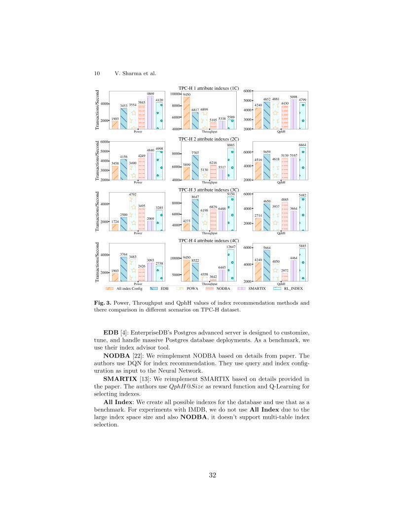
10 V. Sharma et al.

Power

2000

4000Tr

ansa

ction

s/Sec

ond

1903

3453 3554 3845

48694120

Throughput4000

6000

8000

10000 9450

6817 6899

5105 5338 5589

TPC-H 1 attribute indexes (1C)

QphH2000

3000

4000

5000

6000

42404852 4881

44305098

4799

Power2000

3000

4000

5000

6000

Tran

sacti

ons/S

econ

d

34584156

3490

42494840 4998

Throughput4000

6000

8000

5899

7707

5130

62165517

8885TPC-H 2 attribute indexes (2C)

QphH2000

4000

6000

4516

5659

46185139 5167

6664

Power

2000

4000

Tran

sacti

ons/S

econ

d

1724

2500

4792

3495

2069

3285

Throughput

4000

6000

8000

4273

8647

61986829 6488

9150TPC-H 3 attribute indexes (3C)

QphH

2000

4000

6000

2714

46503937

4885

3664

5482

Power

2000

4000

Tran

sacti

ons/S

econ

d

1903

3764 3483

24263093

2738

Throughput

5000

10000 94508522

4358 3642

6445

12647TPC-H 4 attribute indexes (4C)

QphH2000

4000

6000

4240

5664

4050

2972

4464

5885

All index Config EDB POWA NODBA SMARTIX RL_INDEX

Fig. 3. Power, Throughput and QphH values of index recommendation methods andthere comparison in different scenarios on TPC-H dataset.

EDB [4]: EnterpriseDB’s Postgres advanced server is designed to customize,tune, and handle massive Postgres database deployments. As a benchmark, weuse their index advisor tool.

NODBA [22]: We reimplement NODBA based on details from paper. Theauthors use DQN for index recommendation. They use query and index config-uration as input to the Neural Network.

SMARTIX [13]: We reimplement SMARTIX based on details provided inthe paper. The authors use QphH@Size as reward function and Q-Learning forselecting indexes.

All Index: We create all possible indexes for the database and use that as abenchmark. For experiments with IMDB, we do not use All Index due to thelarge index space size and also NODBA, it doesn’t support multi-table indexselection.

32

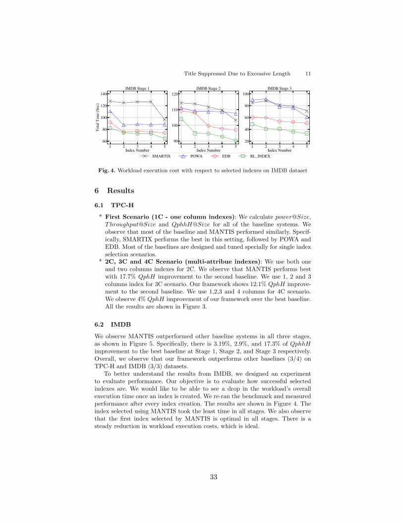
Title Suppressed Due to Excessive Length 11

1 2 3 4 5Index Number

60

80

100

120

140To

tal T

ime (

Sec)

IMDB Stage 1

1 2 3 4 5Index Number

90

100

110

120IMDB Stage 2

1 2 3 4 5Index Number

20

40

60

80

100IMDB Stage 3

SMARTIX POWA EDB RL_INDEX

Fig. 4. Workload execution cost with respect to selected indexes on IMDB dataset

6 Results

6.1 TPC-H

* First Scenario (1C - one column indexes): We calculate power@Size,Throughput@Size and QphhH@Size for all of the baseline systems. Weobserve that most of the baseline and MANTIS performed similarly. Specif-ically, SMARTIX performs the best in this setting, followed by POWA andEDB. Most of the baselines are designed and tuned specially for single indexselection scenarios.

* 2C, 3C and 4C Scenario (multi-attribue indexes): We use both oneand two columns indexes for 2C. We observe that MANTIS performs bestwith 17.7% QphH improvement to the second baseline. We use 1, 2 and 3columns index for 3C scenario. Our framework shows 12.1% QphH improve-ment to the second baseline. We use 1,2,3 and 4 columns for 4C scenario.We observe 4% QphH improvement of our framework over the best baseline.All the results are shown in Figure 3.

6.2 IMDB

We observe MANTIS outperformed other baseline systems in all three stages,as shown in Figure 5. Specifically, there is 3.19%, 2.9%, and 17.3% of QphhHimprovement to the best baseline at Stage 1, Stage 2, and Stage 3 respectively.Overall, we observe that our framework outperforms other baselines (3/4) onTPC-H and IMDB (3/3) datasets.

To better understand the results from IMDB, we designed an experimentto evaluate performance. Our objective is to evaluate how successful selectedindexes are. We would like to be able to see a drop in the workload’s overallexecution time once an index is created. We re-ran the benchmark and measuredperformance after every index creation. The results are shown in Figure 4. Theindex selected using MANTIS took the least time in all stages. We also observethat the first index selected by MANTIS is optimal in all stages. There is asteady reduction in workload execution costs, which is ideal.

33

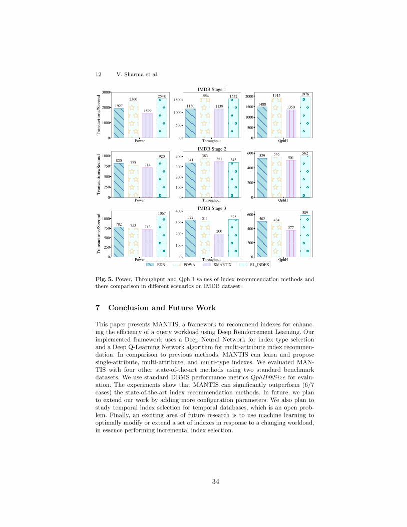
12 V. Sharma et al.

Power0

1000

2000

3000Tr

ansa

ction

s/Sec

ond

19272360

1599

2548

Throughput0

500

1000

15001150

1554

1139

1532IMDB Stage 1

QphH0

500

1000

1500

2000

1488

1915

1350

1976

Power0

250

500

750

1000

Tran

sacti

ons/S

econ

d

820 778 714

920

Throughput0

100

200

300

400341

383351 343

IMDB Stage 2

QphH0

200

400

600 529 546501

562

Power0

250

500

750

1000

Tran

sacti

ons/S

econ

d

782 753 713

1067

Throughput0

100

200

300

400322 311

200

325

IMDB Stage 3

QphH0

200

400

600502 484

377

589

EDB POWA SMARTIX RL_INDEX

Fig. 5. Power, Throughput and QphH values of index recommendation methods andthere comparison in different scenarios on IMDB dataset.

7 Conclusion and Future Work

This paper presents MANTIS, a framework to recommend indexes for enhanc-ing the efficiency of a query workload using Deep Reinforcement Learning. Ourimplemented framework uses a Deep Neural Network for index type selectionand a Deep Q-Learning Network algorithm for multi-attribute index recommen-dation. In comparison to previous methods, MANTIS can learn and proposesingle-attribute, multi-attribute, and multi-type indexes. We evaluated MAN-TIS with four other state-of-the-art methods using two standard benchmarkdatasets. We use standard DBMS performance metrics QphH@Size for evalu-ation. The experiments show that MANTIS can significantly outperform (6/7cases) the state-of-the-art index recommendation methods. In future, we planto extend our work by adding more configuration parameters. We also plan tostudy temporal index selection for temporal databases, which is an open prob-lem. Finally, an exciting area of future research is to use machine learning tooptimally modify or extend a set of indexes in response to a changing workload,in essence performing incremental index selection.

34

Title Suppressed Due to Excessive Length 13

References

1. Basu, D., Lin, Q., Chen, W., Vo, H.T., Yuan, Z., Senellart, P., Bressan, S.:Cost-model oblivious database tuning with reinforcement learning. In: DEXA. p.253–268. DEXA 2015, Springer-Verlag, Berlin, Heidelberg (2015)

2. Ding, B., Das, S., Marcus, R., Wu, W., Chaudhuri, S., Narasayya, V.R.: AI meetsAI: Leveraging query executions to improve index recommendations. In: SIGMOD.p. 1241–1258 (2019)

3. Durand, G.C., Pinnecke, M., Piriyev, R., Mohsen, M., Broneske, D., Saake, G.,Sekeran, M.S., Rodriguez, F., Balami, L.: Gridformation: Towards self-driven on-line data partitioning using reinforcement learning. In: aiDM’18 (2018)

4. EDB: Enterprise Database (EDB): Power to Postgres (2020),https://www.enterprisedb.com/

5. Hilprecht, B., Binnig, C., Rohm, U.: Towards learning a partitioningadvisor with deep reinforcement learning. In: Proceedings of the Sec-ond International Workshop on Exploiting Artificial Intelligence Techniquesfor Data Management. aiDM ’19, Association for Computing Machin-ery, New York, NY, USA (2019). https://doi.org/10.1145/3329859.3329876,https://doi.org/10.1145/3329859.3329876

6. Kllapi, H., Pietri, I., Kantere, V., Ioannidis, Y.E.: Automated management ofindexes for dataflow processing engines in iaas clouds. In: EDBT. pp. 169–180(2020)

7. Krishnan, S., Yang, Z., Goldberg, K., Hellerstein, J., Stoica, I.: Learning to optimizejoin queries with deep reinforcement learning (2018)

8. Krishnan, S., Yang, Z., Goldberg, K., Hellerstein, J.M., Stoica, I.: Learning tooptimize join queries with deep reinforcement learning. CoRR abs/1808.03196(2018), http://arxiv.org/abs/1808.03196

9. Lan, H., Bao, Z., Peng, Y.: An index advisor using deep reinforcement learning. In:Proceedings of the 29th ACM International Conference on Information & Knowl-edge Management. pp. 2105–2108 (2020)

10. Leis, V., Gubichev, A., Mirchev, A., Boncz, P., Kemper, A., Neu-mann, T.: How good are query optimizers, really? Proc. VLDB En-dow. 9(3), 204–215 (Nov 2015). https://doi.org/10.14778/2850583.2850594,http://dx.doi.org/10.14778/2850583.2850594

11. Li, G., Zhou, X., Li, S., Gao, B.: Qtune: A query-aware database tun-ing system with deep reinforcement learning. Proc. VLDB Endow.12(12), 2118–2130 (Aug 2019). https://doi.org/10.14778/3352063.3352129,https://doi.org/10.14778/3352063.3352129

12. Li, Y.: Deep reinforcement learning: An overview. CoRR abs/1701.07274 (2017),http://arxiv.org/abs/1701.07274

13. Licks, G.P., Couto, J.C., de Fatima Miehe, P., De Paris, R., Ruiz, D.D., Meneguzzi,F.: Smartix: A database indexing agent based on reinforcement learning. AppliedIntelligence pp. 1–14 (2020)

14. Ma, Q., Ge, S., He, D., Thaker, D., Drori, I.: Combinatorial optimization by graphpointer networks and hierarchical reinforcement learning (2019)

15. Marcus, R., Papaemmanouil, O.: Deep reinforcement learning for join order enu-meration. In: Proceedings of the First International Workshop on ExploitingArtificial Intelligence Techniques for Data Management. pp. 3:1–3:4. aiDM’18,ACM, New York, NY, USA (2018). https://doi.org/10.1145/3211954.3211957,http://doi.acm.org/10.1145/3211954.3211957

35

14 V. Sharma et al.

16. Marcus, R., Papaemmanouil, O.: Towards a hands-free query optimizer throughdeep learning. CoRR abs/1809.10212 (2018), http://arxiv.org/abs/1809.10212

17. Nazari, M., Oroojlooy, A., Snyder, L., Takac, M.: Reinforcement learning for solv-ing the vehicle routing problem. In: Advances in Neural Information ProcessingSystems. pp. 9839–9849 (2018)

18. Ortiz, J., Balazinska, M., Gehrke, J., Keerthi, S.S.: Learning state representationsfor query optimization with deep reinforcement learning. In: Proceedings of theSecond Workshop on Data Management for End-To-End Machine Learning. pp. 1–4 (2018)

19. Piatetsky-Shapiro, G.: The optimal selection of secondary indices is np-complete.SIGMOD Rec. 13(2), 72–75 (Jan 1983)

20. Powa-Team: PostgreSQL Workload Analyzer (Powa) (2020),https://github.com/powa-team/powa

21. Sadri, Z., Gruenwald, L., Lead, E.: Drlindex: Deep reinforcementlearning index advisor for a cluster database. In: Proceedings ofthe 24th Symposium on International Database Engineering & Ap-plications. IDEAS ’20, Association for Computing Machinery, NewYork, NY, USA (2020). https://doi.org/10.1145/3410566.3410603,https://doi.org/10.1145/3410566.3410603

22. Sharma, A., Schuhknecht, F.M., Dittrich, J.: The case for automatic databaseadministration using deep reinforcement learning. CoRR abs/1801.05643 (2018),http://arxiv.org/abs/1801.05643

23. TPC-H: TPC-H Decision Support Benchmark (2020), http://www.tpc.org/tpch/24. Trummer, I., Moseley, S., Maram, D., Jo, S., Antonakakis, J.: Skinnerdb:

Regret-bounded query evaluation via reinforcement learning. Proc. VLDB En-dow. 11(12), 2074–2077 (Aug 2018). https://doi.org/10.14778/3229863.3236263,https://doi.org/10.14778/3229863.3236263

25. Welborn, J., Schaarschmidt, M., Yoneki, E.: Learning index selection with struc-tured action spaces. arXiv preprint arXiv:1909.07440 (2019)

26. Yang, Z., Chandramouli, B., Wang, C., Gehrke, J., Li, Y., Minhas, U.F., Larson,P.r., Kossmann, D., Acharya, R.: Qd-tree: Learning data layouts for big data an-alytics. In: Proceedings of the 2020 ACM SIGMOD International Conference onManagement of Data. p. 193–208. SIGMOD ’20, Association for Computing Ma-chinery, New York, NY, USA (2020). https://doi.org/10.1145/3318464.3389770,https://doi.org/10.1145/3318464.3389770

27. Yu, X., Li, G., Chai, C., Tang, N.: Reinforcement learning with tree-lstm for joinorder selection. In: 2020 IEEE 36th International Conference on Data Engineering(ICDE). pp. 1297–1308 (2020)

28. Zhang, J., Liu, Y., Zhou, K., Li, G., Xiao, Z., Cheng, B., Xing, J.,Wang, Y., Cheng, T., Liu, L., Ran, M., Li, Z.: An end-to-end au-tomatic cloud database tuning system using deep reinforcement learn-ing. In: Proceedings of the 2019 International Conference on Managementof Data. p. 415–432. SIGMOD ’19, Association for Computing Machin-ery, New York, NY, USA (2019). https://doi.org/10.1145/3299869.3300085,https://doi.org/10.1145/3299869.3300085

29. Zhu, S., Ng, I., Chen, Z.: Causal discovery with reinforcement learning. In: Inter-national Conference on Learning Representations (ICLR) (2020)

36

37

CHAPTER 4

Indexer++: Workload-Aware Online Index Tuning Using

Deep Reinforcement Learning

Indexer++: Workload-Aware Online Index Tuning Using DeepReinforcement Learning

Vishal SharmaUtah State University

Department of Computer Sciencevishal.sharma@usu.edu

Curtis DyresonUtah State University

Department of Computer Sciencecurtis.dyreson@usu.edu

ABSTRACTThe optimal set of indexes is a critical component for a high per-formance of the Database Management System (DBMS). The Data-base Administrator (DBA) selects a set of indexes based on histor-ical workload analysis. A modern database processes thousandsof queries per minute. A DBA’s manual index selection for such adatabase is a challenging task. Such a modern database is designedto serve multiple users and applications, and a query workload insuch a database is heterogeneous in nature. With the increasingworkload complexity, the optimal index configuration for such adatabase also varies. The ability to learn and adapt to evolving work-loads is critical for a database performance. This paper proposesan autonomous workload-aware online index selection using DeepReinforcement Learning. Our approach uses a combination of textanalytic techniques and deep reinforcement learning. It consistsof two steps (i) understanding a workload using embeddings. Tosupport generalized workload analytics, we evaluate several Nat-ural Language Processing (NLP) techniques for workload vectorrepresentation. We observe, vector representation using pretrainedtransformer-based NLP models (BERT, Transformer, XLM, etc.) out-performs existing feature-based approaches. We use NLP modelsthat have been pre-trained to detect changes in workload patterns.Specifically, query workloads are embedded using pretrained mod-els and K-medoids are used to cluster historical and future workloadtrends. (ii) index selection, using deep reinforcement learning. Weimprove the performance of Deep Q-Networks (DQN) by utilizingdisk size constraints and handling noisy rewards in our rewardfunction using a 1D convolution filter. We also introduce PriorityExperience Sweeping in a DQN for an online index tuning. We per-form several experiments using benchmark and real life datasetson our framework. We observe that our approach could effectivelydetect changes in workload trends and select indexes in a shortperiod of time.

1 INTRODUCTIONAn important part of setting up a database is choosing a set ofindexes that balances the trade-off between query execution time,storage cost, and update cost [1]. Having too few indexes may slowthe evaluation of some queries while toomanymay increase the costof data update and the size of the database. Though choosing theright set of indexes is critical to achieving good performance [13]selecting an optimal set of indexes, which we will call the indexselection problem, is NP-hard [47].

Conference’17, July 2017, Washington, DC, USA2021. ACM ISBN 978-x-xxxx-xxxx-x/YY/MM. . . $15.00https://doi.org/10.1145/nnnnnnn.nnnnnnn

Historically a database administrator chose the set of indexes,but research in self-managing databases has demonstrated thatautomated index selection can outperform manual selection. Previ-ous research has focused on offline automated methods. An offlineindexer uses the current state of the database and a representativequery workload to determine which indexes to create. Offline index-ers use heuristics [11, 18, 44, 57], machine learning [15, 26, 27, 58],or reinforcement learning [3, 24, 53] to recommend a set of indexes.

The set of indexes generated by an offline indexer can becomestale if the workload or database changes. A stale set can be re-freshed by re-running the offline indexer to recreate the indexes.But the cost of offline indexers can be high (on the order of hoursof computation time) since an algorithm may run thousands ofqueries and build many indexes to determine the optimal set ofindexes. When offline indexers are run once the cost of running thealgorithm is usually a minor concern (the cost is amortized overthe lifetime of the database) but frequent periodic runs can degradeperformance.

In contrast to offline index selection, the goal of online index se-lection is to keep the set of indexes fresh. An online indexer generatesa set of indexes initially and then incrementally adapts the set in re-sponse to trends in workload or database changes. Online indexersface several challenges not shared by their offline counterparts.(C1) Noise Resilience: Online indexers have the problem of how

to identify a trend, e.g., how many new queries does it take toindicate a trend? An online indexer must be able to adapt tochanging trends but avoid short-lived trends since there is acost to building or removing an index. A constantly shiftingset of indexes could worsen DBMS performance.

(C2) Overhead: Cost is a critical concern. The tuning processmust be able to run concurrently with other DBMS oper-ations without adversely impacting workload processing.Low overhead ensures that an online indexer can (in effect)run continuously to respond to changing trends.

(C3) Trend Detection: Trends move fast. An inability to detectthem quickly may result in delayed index creation. Too bigof a delay in trend detection may, in return, reduce the utilityof the indexer.

(C4) Responsiveness: The tuning approach should be able torespond quickly, on the order of minutes, if it takes severalhours or more for index selection the tuning may miss atrend. Ideally an online indexer will be able to achieve real-time responsiveness.

Previous research in online index selection [7, 39, 46, 48, 50]focused on how to analyze a query workload window to generate aset of indexes. These approaches do not adapt to changing workloadpatterns. They also have high cost and so have a long delay between

38

Conference’17, July 2017, Washington, DC, USA Vishal Sharma and Curtis Dyreson

trend detection and index selection. This reduces the utility ofhaving an online index selector.

This paper presents Indexer++, a workload-aware, online in-dexer. The paper makes the following contributions.

• We propose a novel workload trend detection technique usinga pretrained transformer based on a NLP model and a K-medoids clustering algorithm.

• We describe a real-time, online index selection frameworkthat uses Deep Reinforcement Learning to predict trendsand tune the set of indexes.

• We use Reinforcement learning to learn the interactionsbetween indexes [29] that can speed up performance [51].

• We present an extensive evaluation of our framework. Theexperiments demonstrate that framework is able to addresschallenges C1-C4 listed above.

This paper is organized as follows. Section 2 describes relatedwork and Section 3 formulates the problem. In Section 4 we describeour framework, introduce a workload embedding technique, anduse the technique to detect patterns of change in a workload. Thesection also describes our algorithm for online index selection.Section 5 presents experiments, and finally Section 6 concludes thepaper and describes future work.

2 RELATEDWORKThis section explores related work on workload embedding andonline index tuning in DBMSs.

Word Embedding: In the NLP field, obtaining a vector rep-resentation of word (word embedding) has been extensively stud-ied. The idea of such representation was introduced by Hinton etal. [21]. There has been tremendous growth in the NLP researchfield with the applications of Neural Network for extracting embed-dings. Mikolov et al. [42] proposedword2vec a neural network basedmodel that can learn latent relationship between words from a cor-pus of text. This advancement led to solving several challengingproblems of NLP with high accuracy such as semantic analogy [33],sentiment analysis [52], document classification [35] to name a few.The idea was later extended for a sentence and document [31]. Toimprove the vector representation other deep learning techniqueswere also applied such as CNN [40], RNN [37], LSTM [36]. Therewas a significant improvement in the quality of word embeddingwith the introduction of Deep Bidirectional Transformers. Fewmodels based on transforms are Bert [14], Transformer-XL [12],XLM [28]. We use pretrained transformer based models for wordembedding in our framework. Our goal of using word embeddingis to learn the semantic and syntactic relationship between queries.

Query Embedding: There has been several previous approachesto vectorize an SQL query. Bordawekar et al. [5, 6] utilize pre-trainedword2vec models for query embedding and introduce cognitivecapability in databases. Jain et al. [23] performs error prediction,and workload summarization using vector representation learntby training a LSTM based autoencoder. Bandyopadhyay et al. [2]propose a database column embedding using Bi-LSTM for drug-drug interaction (DDI) prediction. Cappuzzo et al. [10] propose dataintegration using graph-based representation. Günther et al. [17]proposes enriching database queries using pre-trained word2vecmodel.

Online index tuning: The problem of online indexing has beenstudied widely. The preliminary work was done by Hammer etal. [19] in the 1970s, where authors use heuristics for index selec-tion on a single table. Frank et al. [16] proposed an online tuningmethod for a single index selection problem using workload statis-tics for change detection and using heuristics for index selection.Kołaczkowski et al. [25] searches for indexes in a query executionplan space and select them using evolution strategy. A solutionusing heuristics may fail in scalability, specifically in challenges(C4). Bruno et al. [8] design a hardcoded rule approach for indexselection. Their approach is fast and scalable, but it lacks noiseresilience (C1). For a small DBMS application such an approachmay work, but it can worsen the performance on a larger system.Schnaitter et al. [50] proposed a very effective online indexingsolution that monitors the incoming queries and minimizes theoverhead cost. Their index selection uses heuristics. For real-timeonline index selection it is slow (C4) and susceptible to noise (C1).Sadri et al. [49] proposed an index tuning algorithm using deepreinforcement learning. As described by the authors, their approachtakes a long time for index selection. Thereby not being able to han-dle the challenge (C4). The previous approaches does not overcomeall challenges. They mostly fail in noise resilience (C1), and scal-ability (C4). Our proposed approach overcomes all the challenges(C1)-(C4). We discuss them in detail in Section 4.3.5.

3 PROBLEM FORMULATIONThe index recommendation problem is to select a set of indexesthat minimizes the time to evaluate a workload and the amountof storage needed. A set of indexes that minimizes the workloadcost with a storage size constraint is a constrained combinatorialoptimization problem.

A workload𝑊 is a set of SQL queries 𝑄1, 𝑄2,.., 𝑄𝑚 . An indexconfiguration 𝐼 is a set of indexes. We calculate the cost of workloadevaluation on database 𝐷 using the cost of the evaluation of eachindividual query given by 𝐶𝑜𝑠𝑡 (𝑄 𝑗 , 𝐼 , 𝐷). The cost of a workloadcan be described as follows.

Cost (𝑊, 𝐼, 𝐷) =𝑚∑𝑗=1

Cost (𝑄 𝑗 , 𝐼 , 𝐷)

Note that the workload cost does not weight queries differently,though we could trivially include such weights by replicating indi-vidual queries in a workload. The index selection problem is to finda set of indexes 𝐼𝑜𝑝𝑡𝑖𝑚𝑎𝑙 that minimizes the total cost of a workload,Cost (𝑊, 𝐼, 𝐷), and has a storage cost of at most 𝐶 .

𝐼optimal = min𝑆 (𝐼 ∗) ≤𝐶

Cost (𝑊, 𝐼∗, 𝐷)

In this equation 𝑆 (𝐼∗) is the total storage space cost of the set ofindexes 𝐼∗. The space constraint is important because index creationshould be parsimonious. Creating more indexes than necessarywastes space and slows data modification.

The online index selection problem can be formulated as follows.Let a workload stream𝑊 ∗ be a sequence of workloads [𝑊1,𝑊2, .. ,𝑊𝑘 ]. Let Diff (𝑊1,𝑊2, ..,𝑊𝑘 ) be a metric that quantifies the differ-ence between workloads in the stream. Then online Index Selectioncan be defined as:

39

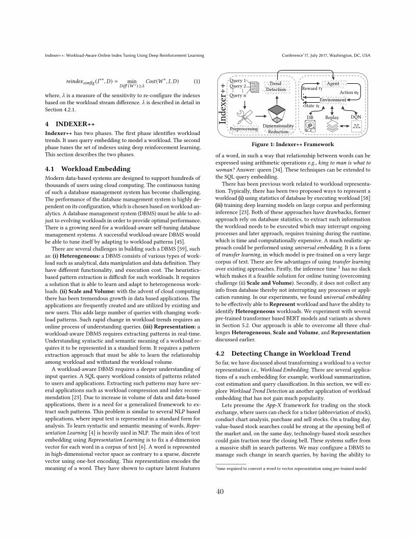
Indexer++: Workload-Aware Online Index Tuning Using Deep Reinforcement Learning Conference’17, July 2017, Washington, DC, USA

reindexconfig (𝐼∗∗, 𝐷) = minDiff (𝑊 ∗) ≥_

Cost (𝑊 ∗, 𝐼 , 𝐷) (1)

where, _ is a measure of the sensitivity to re-configure the indexesbased on the workload stream difference. _ is described in detail inSection 4.2.1.

4 INDEXER++Indexer++ has two phases. The first phase identifies workloadtrends. It uses query embedding to model a workload. The secondphase tunes the set of indexes using deep reinforcement learning.This section describes the two phases.

4.1 Workload EmbeddingModern data-based systems are designed to support hundreds ofthousands of users using cloud computing. The continuous tuningof such a database management system has become challenging.The performance of the database management system is highly de-pendent on its configuration, which is chosen based onworkload an-alytics. A database management system (DBMS) must be able to ad-just to evolving workloads in order to provide optimal performance.There is a growing need for a workload-aware self-tuning databasemanagement systems. A successful workload-aware DBMS wouldbe able to tune itself by adapting to workload patterns [45].

There are several challenges in building such a DBMS [59], suchas: (i) Heterogeneous: a DBMS consists of various types of work-load such as analytical, data manipulation and data definition. Theyhave different functionality, and execution cost. The heuristics-based pattern extraction is difficult for such workloads. It requiresa solution that is able to learn and adapt to heterogeneous work-loads. (ii) Scale and Volume: with the advent of cloud computingthere has been tremendous growth in data based applications. Theapplications are frequently created and are utilized by existing andnew users. This adds large number of queries with changing work-load patterns. Such rapid change in workload trends requires anonline process of understanding queries. (iii) Representation: aworkload-aware DBMS requires extracting patterns in real-time.Understanding syntactic and semantic meaning of a workload re-quires it to be represented in a standard form. It requires a patternextraction approach that must be able to learn the relationshipamong workload and withstand the workload volume.

A workload-aware DBMS requires a deeper understanding ofinput queries. A SQL query workload consists of patterns relatedto users and applications. Extracting such patterns may have sev-eral applications such as workload compression and index recom-mendation [23]. Due to increase in volume of data and data-basedapplications, there is a need for a generalized framework to ex-tract such patterns. This problem is similar to several NLP basedapplications, where input text is represented in a standard form foranalysis. To learn syntactic and semantic meaning of words, Repre-sentation Learning [4] is heavily used in NLP. The main idea of textembedding using Representation Learning is to fix a d-dimensionvector for each word in a corpus of text [6]. A word is representedin high-dimensional vector space as contrary to a sparse, discretevector using one-hot encoding. This representation encodes themeaning of a word. They have shown to capture latent features

Agent

Environment

Action Reward

State

DQNDB Replay

ery 1ery 2

ery n

Trend Detection

PreprocessingDimensionality

Reduction

Inde

xer+

+

Figure 1: Indexer++ Framework

of a word, in such a way that relationship between words can beexpressed using arithmetic operations e.g., king to man is what towoman? Answer: queen [34]. These techniques can be extended tothe SQL query embedding.

There has been previous work related to workload representa-tion. Typically, there has been two proposed ways to represent aworkload (i) using statistics of database by executing workload [58](ii) training deep learning models on large corpus and performinginference [23]. Both of these approaches have drawbacks, formerapproach rely on database statistics, to extract such informationthe workload needs to be executed which may interrupt ongoingprocesses and later approach, requires training during the runtime,which is time and computationally expensive. A much realistic ap-proach could be performed using universal embedding. It is a formof transfer learning, in which model is pre-trained on a very largecorpus of text. There are few advantages of using transfer learningover existing approaches. Firstly, the inference time 1 has no slackwhich makes it a feasible solution for online tuning (overcomingchallenge (ii) Scale and Volume). Secondly, it does not collect anyinfo from database thereby not interrupting any processes or appli-cation running. In our experiments, we found universal embeddingto be effectively able toRepresentworkload and have the ability toidentify Heterogeneous workloads. We experiment with severalpre-trained transformer based BERT models and variants as shownin Section 5.2. Our approach is able to overcome all three chal-lenges Heterogeneous, Scale and Volume, and Representationdiscussed earlier.

4.2 Detecting Change in Workload TrendSo far, we have discussed about transforming a workload to a vectorrepresentation i.e., Workload Embedding. There are several applica-tions of a such embedding for example, workload summarization,cost estimation and query classification. In this section, we will ex-plore Workload Trend Detection an another application of workloadembedding that has not gain much popularity.

Lets presume the App-X framework for trading on the stockexchange, where users can check for a ticker (abbreviation of stock),conduct chart analysis, purchase and sell stocks. On a trading day,value-based stock searches could be strong at the opening bell ofthe market and, on the same day, technology-based stock searchescould gain traction near the closing bell. These systems suffer froma massive shift in search patterns. We may configure a DBMS tomanage such change in search queries, by having the ability to

1time required to convert a word to vector representation using pre-trained model

40

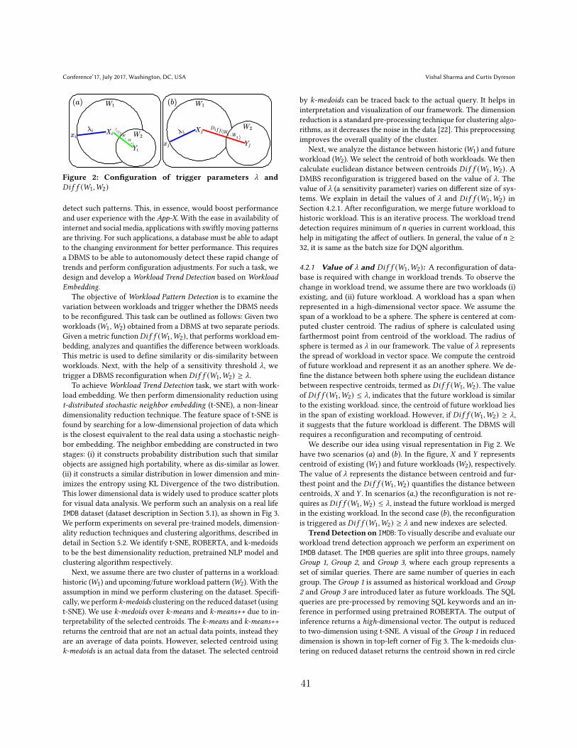
Conference’17, July 2017, Washington, DC, USA Vishal Sharma and Curtis Dyreson

Figure 2: Configuration of trigger parameters _ and𝐷𝑖 𝑓 𝑓 (𝑊1,𝑊2)

detect such patterns. This, in essence, would boost performanceand user experience with the App-X. With the ease in availability ofinternet and social media, applications with swiftly moving patternsare thriving. For such applications, a database must be able to adaptto the changing environment for better performance. This requiresa DBMS to be able to autonomously detect these rapid change oftrends and perform configuration adjustments. For such a task, wedesign and develop a Workload Trend Detection based on WorkloadEmbedding.

The objective of Workload Pattern Detection is to examine thevariation between workloads and trigger whether the DBMS needsto be reconfigured. This task can be outlined as follows: Given twoworkloads (𝑊1,𝑊2) obtained from a DBMS at two separate periods.Given a metric function𝐷𝑖 𝑓 𝑓 (𝑊1,𝑊2), that performs workload em-bedding, analyzes and quantifies the difference between workloads.This metric is used to define similarity or dis-similarity betweenworkloads. Next, with the help of a sensitivity threshold _, wetrigger a DBMS reconfiguration when 𝐷𝑖 𝑓 𝑓 (𝑊1,𝑊2) ≥ _.

To achieveWorkload Trend Detection task, we start with work-load embedding. We then perform dimensionality reduction usingt-distributed stochastic neighbor embedding (t-SNE), a non-lineardimensionality reduction technique. The feature space of t-SNE isfound by searching for a low-dimensional projection of data whichis the closest equivalent to the real data using a stochastic neigh-bor embedding. The neighbor embedding are constructed in twostages: (i) it constructs probability distribution such that similarobjects are assigned high portability, where as dis-similar as lower.(ii) it constructs a similar distribution in lower dimension and min-imizes the entropy using KL Divergence of the two distribution.This lower dimensional data is widely used to produce scatter plotsfor visual data analysis. We perform such an analysis on a real lifeIMDB dataset (dataset description in Section 5.1), as shown in Fig 3.We perform experiments on several pre-trained models, dimension-ality reduction techniques and clustering algorithms, described indetail in Section 5.2. We identify t-SNE, ROBERTA, and k-medoidsto be the best dimensionality reduction, pretrained NLP model andclustering algorithm respectively.

Next, we assume there are two cluster of patterns in a workload:historic (𝑊1) and upcoming/future workload pattern (𝑊2). With theassumption in mind we perform clustering on the dataset. Specifi-cally, we perform k-medoids clustering on the reduced dataset (usingt-SNE). We use k-medoids over k-means and k-means++ due to in-terpretability of the selected centroids. The k-means and k-means++returns the centroid that are not an actual data points, instead theyare an average of data points. However, selected centroid usingk-medoids is an actual data from the dataset. The selected centroid

by k-medoids can be traced back to the actual query. It helps ininterpretation and visualization of our framework. The dimensionreduction is a standard pre-processing technique for clustering algo-rithms, as it decreases the noise in the data [22]. This preprocessingimproves the overall quality of the cluster.

Next, we analyze the distance between historic (𝑊1) and futureworkload (𝑊2). We select the centroid of both workloads. We thencalculate euclidean distance between centroids 𝐷𝑖 𝑓 𝑓 (𝑊1,𝑊2). ADMBS reconfiguration is triggered based on the value of _. Thevalue of _ (a sensitivity parameter) varies on different size of sys-tems. We explain in detail the values of _ and 𝐷𝑖 𝑓 𝑓 (𝑊1,𝑊2) inSection 4.2.1. After reconfiguration, we merge future workload tohistoric workload. This is an iterative process. The workload trenddetection requires minimum of 𝑛 queries in current workload, thishelp in mitigating the affect of outliers. In general, the value of 𝑛 ≥32, it is same as the batch size for DQN algorithm.

4.2.1 Value of _ and 𝐷𝑖 𝑓 𝑓 (𝑊1,𝑊2): A reconfiguration of data-base is required with change in workload trends. To observe thechange in workload trend, we assume there are two workloads (i)existing, and (ii) future workload. A workload has a span whenrepresented in a high-dimensional vector space. We assume thespan of a workload to be a sphere. The sphere is centered at com-puted cluster centroid. The radius of sphere is calculated usingfarthermost point from centroid of the workload. The radius ofsphere is termed as _ in our framework. The value of _ representsthe spread of workload in vector space. We compute the centroidof future workload and represent it as an another sphere. We de-fine the distance between both sphere using the euclidean distancebetween respective centroids, termed as 𝐷𝑖 𝑓 𝑓 (𝑊1,𝑊2). The valueof 𝐷𝑖 𝑓 𝑓 (𝑊1,𝑊2) ≤ _, indicates that the future workload is similarto the existing workload. since, the centroid of future workload liesin the span of existing workload. However, if 𝐷𝑖 𝑓 𝑓 (𝑊1,𝑊2) ≥ _,it suggests that the future workload is different. The DBMS willrequires a reconfiguration and recomputing of centroid.

We describe our idea using visual representation in Fig 2. Wehave two scenarios (𝑎) and (𝑏). In the figure, 𝑋 and 𝑌 representscentroid of existing (𝑊1) and future workloads (𝑊2), respectively.The value of _ represents the distance between centroid and fur-thest point and the 𝐷𝑖 𝑓 𝑓 (𝑊1,𝑊2) quantifies the distance betweencentroids, 𝑋 and 𝑌 . In scenarios (𝑎,) the reconfiguration is not re-quires as 𝐷𝑖 𝑓 𝑓 (𝑊1,𝑊2) ≤ _, instead the future workload is mergedin the existing workload. In the second case (𝑏), the reconfigurationis triggered as 𝐷𝑖 𝑓 𝑓 (𝑊1,𝑊2) ≥ _ and new indexes are selected.

Trend Detection on IMDB: To visually describe and evaluate ourworkload trend detection approach we perform an experiment onIMDB dataset. The IMDB queries are split into three groups, namelyGroup 1, Group 2, and Group 3, where each group represents aset of similar queries. There are same number of queries in eachgroup. The Group 1 is assumed as historical workload and Group2 and Group 3 are introduced later as future workloads. The SQLqueries are pre-processed by removing SQL keywords and an in-ference in performed using pretrained ROBERTA. The output ofinference returns a high-dimensional vector. The output is reducedto two-dimension using t-SNE. A visual of the Group 1 in reduceddimension is shown in top-left corner of Fig 3. The k-medoids clus-tering on reduced dataset returns the centroid shown in red circle

41

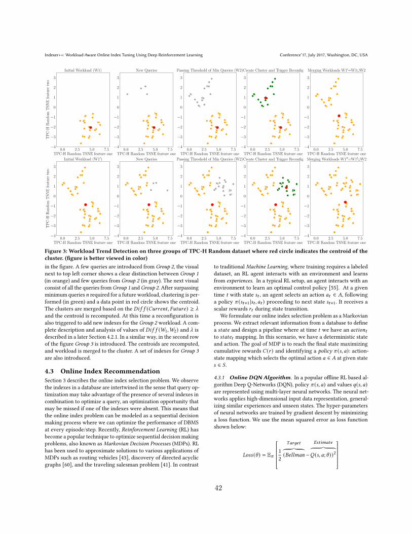
Indexer++: Workload-Aware Online Index Tuning Using Deep Reinforcement Learning Conference’17, July 2017, Washington, DC, USA

0.0 2.5 5.0 7.5TPC-H Random TSNE feature one

−4

−3

−2

−1

0

1

2

3

TP

C-H

Ran

dom

TS

NE

feat

ure

two

Initial Workload (W1)

0.0 2.5 5.0 7.5TPC-H Random TSNE feature one

−4

−3

−2

−1

0

1

2

3

New Queries

0.0 2.5 5.0 7.5TPC-H Random TSNE feature one

−4

−3

−2

−1

0

1

2

3

Passing Threshold of Min Queries (W2)

0.0 2.5 5.0 7.5TPC-H Random TSNE feature one

−4

−3

−2

−1

0

1

2

3

Create Cluster and Trigger Reconfig

0.0 2.5 5.0 7.5TPC-H Random TSNE feature one

−4

−3

−2

−1

0

1

2

3

Merging Workloads W1′=W1∪W2

0.0 2.5 5.0 7.5TPC-H Random TSNE feature one

−4

−3

−2

−1

0

1

2

3

TP

C-H

Ran

dom

TS

NE

feat

ure

two

Initial Workload (W1′)

0.0 2.5 5.0 7.5TPC-H Random TSNE feature one

−4

−3

−2

−1

0

1

2

3

New Queries

0.0 2.5 5.0 7.5TPC-H Random TSNE feature one

−4

−3

−2

−1

0

1

2

3

Passing Threshold of Min Queries (W2)

0.0 2.5 5.0 7.5TPC-H Random TSNE feature one

−4

−3

−2

−1

0

1

2

3

Create Cluster and Trigger Reconfig

0.0 2.5 5.0 7.5TPC-H Random TSNE feature one

−4

−3

−2

−1

0

1

2

3

Merging Workloads W1′′=W1′∪W2

Figure 3: Workload Trend Detection on three groups of TPC-H Random dataset where red circle indicates the centroid of thecluster. (figure is better viewed in color)in the figure. A few queries are introduced from Group 2, the visualnext to top left corner shows a clear distinction between Group 1(in orange) and few queries from Group 2 (in gray). The next visualconsist of all the queries from Group 1 and Group 2. After surpassingminimum queries𝑛 required for a future workload, clustering is per-formed (in green) and a data point in red circle shows the centroid.The clusters are merged based on the 𝐷𝑖 𝑓 𝑓 (𝐶𝑢𝑟𝑟𝑒𝑛𝑡, 𝐹𝑢𝑡𝑢𝑟𝑒) ≥ _and the centroid is recomputed. At this time a reconfiguration isalso triggered to add new indexes for the Group 2 workload. A com-plete description and analysis of values of 𝐷𝑖 𝑓 𝑓 (𝑊1,𝑊2) and _ isdescribed in a later Section 4.2.1. In a similar way, in the second rowof the figure Group 3 is introduced. The centroids are recomputed,and workload is merged to the cluster. A set of indexes for Group 3are also introduced.

4.3 Online Index RecommendationSection 3 describes the online index selection problem. We observethe indexes in a database are intertwined in the sense that query op-timization may take advantage of the presence of several indexes incombination to optimize a query, an optimization opportunity thatmay be missed if one of the indexes were absent. This means thatthe online index problem can be modeled as a sequential decisionmaking process where we can optimize the performance of DBMSat every episode/step. Recently, Reinforcement Learning (RL) hasbecome a popular technique to optimize sequential decision makingproblems, also known as Markovian Decision Processes (MDPs). RLhas been used to approximate solutions to various applications ofMDPs such as routing vehicles [43], discovery of directed acyclicgraphs [60], and the traveling salesman problem [41]. In contrast

to traditional Machine Learning, where training requires a labeleddataset, an RL agent interacts with an environment and learnsfrom experiences. In a typical RL setup, an agent interacts with anenvironment to learn an optimal control policy [55]. At a giventime t with state 𝑠𝑡 , an agent selects an action 𝑎𝑡 ∈ 𝐴, followinga policy 𝜋 (𝑠𝑡+1 |𝑠𝑡 , 𝑎𝑡 ) proceeding to next state 𝑠𝑡+1. It receives ascalar rewards 𝑟𝑡 during state transition.

We formulate our online index selection problem as a Markovianprocess. We extract relevant information from a database to definea 𝑠𝑡𝑎𝑡𝑒 and design a pipeline where at time 𝑡 we have an 𝑎𝑐𝑡𝑖𝑜𝑛𝑡to 𝑠𝑡𝑎𝑡𝑒𝑡 mapping. In this scenario, we have a deterministic stateand action. The goal of MDP is to reach the final state maximizingcumulative rewards 𝐶 (𝑟 ) and identifying a policy 𝜋 (𝑠, 𝑎): action-state mapping which selects the optimal action 𝑎 ∈ 𝐴 at given state𝑠 ∈ 𝑆 .

4.3.1 Online DQN Algorithm. In a popular offline RL based al-gorithm Deep Q-Networks (DQN), policy 𝜋 (𝑠, 𝑎) and values 𝑞(𝑠, 𝑎)are represented using multi-layer neural networks. The neural net-works applies high-dimensional input data representation, general-izing similar experiences and unseen states. The hyper-parametersof neural networks are trained by gradient descent by minimizinga loss function. We use the mean squared error as loss functionshown below:

𝐿𝑜𝑠𝑠 (\ ) = E𝜋

12

𝑇𝑎𝑟𝑔𝑒𝑡︷ ︸︸ ︷(𝐵𝑒𝑙𝑙𝑚𝑎𝑛 −

𝐸𝑠𝑡𝑖𝑚𝑎𝑡𝑒︷ ︸︸ ︷𝑄 (𝑠, 𝑎;\ ))2

42

Conference’17, July 2017, Washington, DC, USA Vishal Sharma and Curtis Dyreson

−5 0 5TSNE Random feature space one

−2

0

2

4

6

8

TS

NE

Ran

dom

feat

ure

spac

etw

o

Initial workload (W1)

−5 0 5TSNE Random feature space one

−2

0

2

4

6

8

New Queries & Recompute Centroid

−5 0 5TSNE Random feature space one

−2

0

2

4

6

8

New Queries & Recompute Centroid

−5 0 5TSNE Random feature space one

−2

0

2

4

6

8

New Queries & Recompute Centroid

−5 0 5TSNE Random feature space one

−2

0

2

4

6

8

New Queries & Recompute Centroid

Figure 4: Workload Trend Detection on TPC-H dataset. It is a scenario when no re-configurations of indexes is trigger. The newqueries are similar to existing workload. The red circle indicates the centroid of the cluster. The existing workload is displayedin orange and new queries are in gray. (figure is better viewed in color)

where \ is a parameter for a nonlinear function, in our casea neural network. Expanding the above equation using BellmanOptimality equation [56] we get:

𝐿𝑜𝑠𝑠 (\ ) = E𝜋

12

©­­­«(𝑅𝑒𝑤𝑎𝑟𝑑︷ ︸︸ ︷𝑅(𝑠, 𝑎) +

𝐹𝑢𝑡𝑢𝑟𝑒 𝑅𝑒𝑤𝑎𝑟𝑑︷ ︸︸ ︷𝛽 max𝑎′∈𝐴

𝑄 (𝑠 ′, 𝑎′;\ )) −𝐸𝑠𝑡𝑖𝑚𝑎𝑡𝑒︷ ︸︸ ︷𝑄 (𝑠, 𝑎;\ )

ª®®®¬

2where, 𝛽 is the discount rate. In above equation, we approachto learn weights of 𝑄 (𝑠, 𝑎;\ ). We use gradient descent optimiza-tion algorithm to learn the parameters and a gradient update w.r.t𝑄 (𝑠, 𝑎;\ ) can be perform using below:

𝑄 (𝑠, 𝑎;\ ) = 𝑄 (𝑠, 𝑎;\ ) − 𝛼𝜕

𝜕𝑄 (𝑠, 𝑎;\ ) 𝐿𝑜𝑠𝑠 (\ )

replacing 𝐿𝑜𝑠𝑠 (\ ) and taking a partial derivative yields:

𝑄 (𝑠, 𝑎;\ ) = 𝑄 (𝑠, 𝑎;\ ) + 𝛼

©­­­­­­«

𝑇𝐷 𝑇𝑎𝑟𝑔𝑒𝑡︷ ︸︸ ︷𝑅(𝑠, 𝑎) + 𝛽 max

𝑎′∈𝐴𝑄 (𝑠 ′, 𝑎′;\ ) −

𝐸𝑠𝑡𝑖𝑚𝑎𝑡𝑒︷ ︸︸ ︷𝑄 (𝑠, 𝑎;\ )︸ ︷︷ ︸

𝑇𝑒𝑚𝑝𝑜𝑟𝑎𝑙 𝐷𝑖 𝑓 𝑓 𝑒𝑟𝑒𝑛𝑐𝑒 (𝑇𝐷) 𝐸𝑟𝑟𝑜𝑟

ª®®®®®®¬Rearranging the above equation gives:

𝑄 (𝑠, 𝑎;\ ) = (1 − 𝛼) 𝑄 (𝑠, 𝑎;\ ) + 𝛼

(𝑅(𝑠, 𝑎) + 𝛽 max

𝑎′∈𝐴𝑄 (𝑠 ′, 𝑎′;\ )

)

We use above equation to generalize the approximation of the Q-value function. A neural network training assumes that input dataare independent and sampled from similar distributions. A neuralnetwork will overfit/underfit if such assumptions are not satisfied.For Reinforcement Learning, we can observe that the target𝑄 valuedepends on itself, making training on a neural network difficultsince it would chase a non-stationary target. To solve this problem,we implement a target network \ ′, which stays stationary for acertain period and later synchronizes with \ . The above equationcan be re-written using target network \ ′ as follows:

𝑄 (𝑠, 𝑎;\ ) = (1 − 𝛼)𝑄 (𝑠, 𝑎;\ ) + 𝛼

(𝑅(𝑠, 𝑎) + 𝛽 max

𝑎′∈𝐴𝑄 (𝑠 ′, 𝑎′;\ ′)

)︸ ︷︷ ︸

𝑇𝐷 𝑇𝑎𝑟𝑔𝑒𝑡

4.3.2 DBMS representation: A state of a DQN agent representsan environment. A state representation should be able to describethe environment to the finest detail. It is a crucial component forlearning an optimal policy.We use index configuration of a DBMS asstate representation. Specifically, index configuration is representedin a one-dimensional vector. In the vector, a binary value representspresence and absence of an index. The length of vector is definedby the value of all possible index configuration (2𝑁𝑐𝑜𝑙𝑢𝑚𝑛𝑠 − 1). Theaction space represents all possible index configuration actions thatcan be performed and is also the same size as state space. A rewardfunction is an another crucial component of the learning process ofDQN agent. It defines a cost function for the agent, with a goal tomaximize. We define our reward function as below:

𝑟𝑒𝑤𝑎𝑟𝑑𝑠𝑠𝑖𝑧𝑒 =

(1 index size < max allowed size

−1 otherwise

)

𝑟𝑡 = max(

index costall index cost − 1, 0

)+ 𝑟𝑒𝑤𝑎𝑟𝑑𝑠𝑠𝑖𝑧𝑒 (2)

where, numerator is the workload cost with selected index anddenominator is workload cost with all index configuration. Ourreward function is designed such that it will have minimum value of-1 and maximum of 10-20, such smaller range of rewards suppressesthe noise while training Neural Network. We also introduce thereward for disk size constraint, where total size of selected indexesis upper bounded with𝑚𝑎𝑥_𝑎𝑙𝑙𝑜𝑤𝑒𝑑_𝑠𝑖𝑧𝑒 e.g.,. 10MB. Our rewardfunction is generic and can be modified for any other constraints.

4.3.3 Priority Experience Replay: A Reinforcement Learningalgorithm updates while interacting with the environment. In sucha situation, the algorithm tends to forget experiences after a fewepochs of training. To solve this problem, we store a buffer calledExperience Replay, which is used to sample from previous experi-ences. It also breaks the temporal dependency otherwise found inregular updates while interacting with environment. ExperienceReplay can lead to slow convergence because data is sampled uni-formly. A previous experience with a large estimated error mayor may not be in sampled data, making the convergence slower.To solve this problem, we use Priority Experience Replay, whereinstead of sampling uniformly, samples are giving importance. Weuse Temporal Difference Error to prioritize experiences:

43

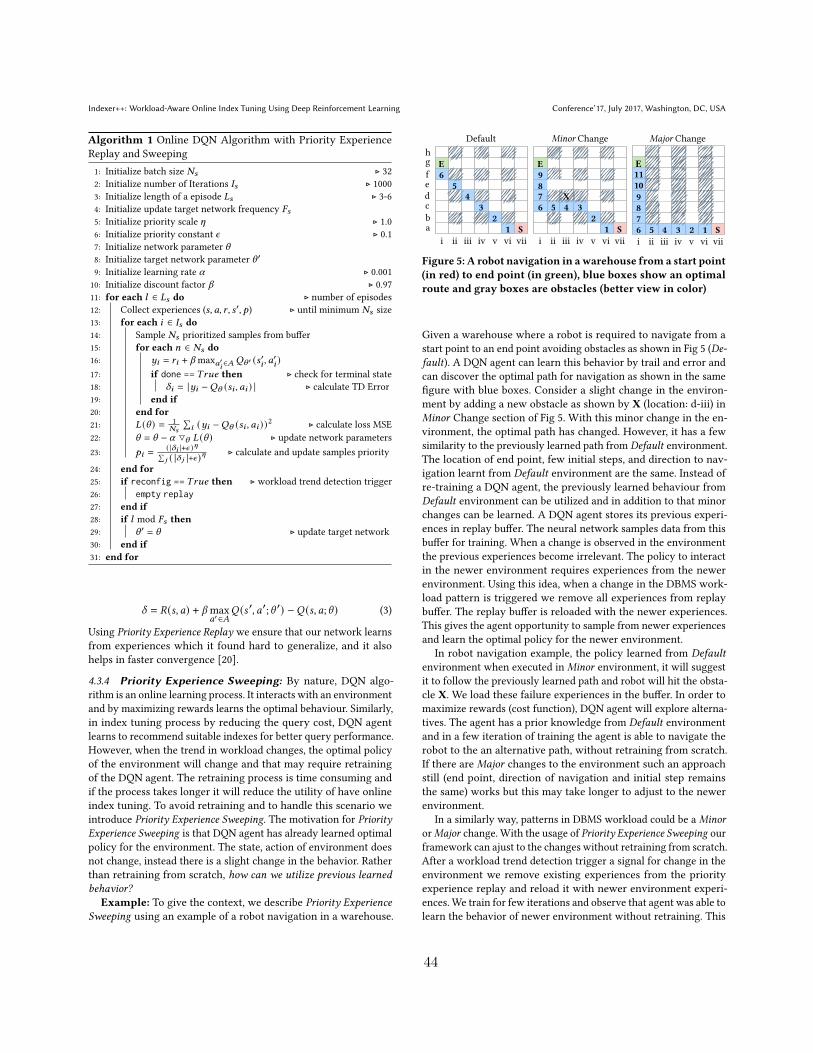
Indexer++: Workload-Aware Online Index Tuning Using Deep Reinforcement Learning Conference’17, July 2017, Washington, DC, USA

Algorithm 1 Online DQN Algorithm with Priority ExperienceReplay and Sweeping1: Initialize batch size 𝑁𝑠 ⊲ 322: Initialize number of Iterations 𝐼𝑠 ⊲ 10003: Initialize length of a episode 𝐿𝑠 ⊲ 3-64: Initialize update target network frequency 𝐹𝑠5: Initialize priority scale [ ⊲ 1.06: Initialize priority constant 𝜖 ⊲ 0.17: Initialize network parameter \8: Initialize target network parameter \ ′9: Initialize learning rate 𝛼 ⊲ 0.00110: Initialize discount factor 𝛽 ⊲ 0.9711: for each 𝑙 ∈ 𝐿𝑠 do ⊲ number of episodes12: Collect experiences (𝑠, 𝑎, 𝑟, 𝑠′, 𝑝) ⊲ until minimum 𝑁𝑠 size13: for each 𝑖 ∈ 𝐼𝑠 do14: Sample 𝑁𝑠 prioritized samples from buffer15: for each 𝑛 ∈ 𝑁𝑠 do16: 𝑦𝑖 = 𝑟𝑖 + 𝛽 max𝑎′𝑖 ∈𝐴𝑄\ ′ (𝑠′𝑖 , 𝑎′𝑖 )17: if done ==𝑇𝑟𝑢𝑒 then ⊲ check for terminal state18: 𝛿𝑖 = |𝑦𝑖 −𝑄\ (𝑠𝑖 , 𝑎𝑖 ) | ⊲ calculate TD Error19: end if20: end for21: 𝐿 (\ ) = 1

𝑁𝑠

∑𝑖 (𝑦𝑖 −𝑄\ (𝑠𝑖 , 𝑎𝑖 ))2 ⊲ calculate loss MSE

22: \ = \ − 𝛼 ▽\ 𝐿 (\ ) ⊲ update network parameters23: 𝑝𝑖 =

( |𝛿𝑖 |+𝜖 )[∑𝑗 ( |𝛿 𝑗 |+𝜖)[ ⊲ calculate and update samples priority

24: end for25: if reconfig ==𝑇𝑟𝑢𝑒 then ⊲ workload trend detection trigger26: empty replay27: end if28: if 𝑙 mod 𝐹𝑠 then29: \ ′ = \ ⊲ update target network30: end if31: end for

𝛿 = 𝑅(𝑠, 𝑎) + 𝛽 max𝑎′∈𝐴

𝑄 (𝑠 ′, 𝑎′;\ ′) −𝑄 (𝑠, 𝑎;\ ) (3)

Using Priority Experience Replay we ensure that our network learnsfrom experiences which it found hard to generalize, and it alsohelps in faster convergence [20].

4.3.4 Priority Experience Sweeping: By nature, DQN algo-rithm is an online learning process. It interacts with an environmentand by maximizing rewards learns the optimal behaviour. Similarly,in index tuning process by reducing the query cost, DQN agentlearns to recommend suitable indexes for better query performance.However, when the trend in workload changes, the optimal policyof the environment will change and that may require retrainingof the DQN agent. The retraining process is time consuming andif the process takes longer it will reduce the utility of have onlineindex tuning. To avoid retraining and to handle this scenario weintroduce Priority Experience Sweeping. The motivation for PriorityExperience Sweeping is that DQN agent has already learned optimalpolicy for the environment. The state, action of environment doesnot change, instead there is a slight change in the behavior. Ratherthan retraining from scratch, how can we utilize previous learnedbehavior?

Example: To give the context, we describe Priority ExperienceSweeping using an example of a robot navigation in a warehouse.

E6

54

32

1 S

E987 X6 5 4 3

21 Sa

bcdefgh

i ii iii iv v vi vii

E11109876 5 4 3 2 1 S

Major ChangeMinor ChangeDefault

i ii iii iv v vi vii i ii iii iv v vi vii

Figure 5: A robot navigation in awarehouse from a start point(in red) to end point (in green), blue boxes show an optimalroute and gray boxes are obstacles (better view in color)

Given a warehouse where a robot is required to navigate from astart point to an end point avoiding obstacles as shown in Fig 5 (De-fault). A DQN agent can learn this behavior by trail and error andcan discover the optimal path for navigation as shown in the samefigure with blue boxes. Consider a slight change in the environ-ment by adding a new obstacle as shown by X (location: d-iii) inMinor Change section of Fig 5. With this minor change in the en-vironment, the optimal path has changed. However, it has a fewsimilarity to the previously learned path from Default environment.The location of end point, few initial steps, and direction to nav-igation learnt from Default environment are the same. Instead ofre-training a DQN agent, the previously learned behaviour fromDefault environment can be utilized and in addition to that minorchanges can be learned. A DQN agent stores its previous experi-ences in replay buffer. The neural network samples data from thisbuffer for training. When a change is observed in the environmentthe previous experiences become irrelevant. The policy to interactin the newer environment requires experiences from the newerenvironment. Using this idea, when a change in the DBMS work-load pattern is triggered we remove all experiences from replaybuffer. The replay buffer is reloaded with the newer experiences.This gives the agent opportunity to sample from newer experiencesand learn the optimal policy for the newer environment.

In robot navigation example, the policy learned from Defaultenvironment when executed in Minor environment, it will suggestit to follow the previously learned path and robot will hit the obsta-cle X. We load these failure experiences in the buffer. In order tomaximize rewards (cost function), DQN agent will explore alterna-tives. The agent has a prior knowledge from Default environmentand in a few iteration of training the agent is able to navigate therobot to the an alternative path, without retraining from scratch.If there are Major changes to the environment such an approachstill (end point, direction of navigation and initial step remainsthe same) works but this may take longer to adjust to the newerenvironment.

In a similarly way, patterns in DBMS workload could be a MinororMajor change. With the usage of Priority Experience Sweeping ourframework can ajust to the changes without retraining from scratch.After a workload trend detection trigger a signal for change in theenvironment we remove existing experiences from the priorityexperience replay and reload it with newer environment experi-ences. We train for few iterations and observe that agent was able tolearn the behavior of newer environment without retraining. This

44

Conference’17, July 2017, Washington, DC, USA Vishal Sharma and Curtis Dyreson

Algorithm 2 Random Query Generator1: Initialize maximum number of columns in a query𝐶 ⊲ 1-42: Initialize number of queries𝑄 ⊲ 1003: for each 𝑞 ∈ 𝑄 do ⊲ number of queries4: for each 𝑐 ∈ 𝐶 do ⊲ number of columns5: Randomly extract a distinct value6: Randomly select operator [>, <, =, =>, <=]7: Randomly select predicates [𝑎𝑛𝑑 , 𝑜𝑟 ]8: Append 𝑞9: end for10: end for

process makes our framework a generic tool for online configura-tion tuning. The complete DQN algorithm with Priority ExperienceReplay and Priority Experience Sweeping is shown in Algorithm 1.

4.3.5 OvercomingChallenges: In Section ??, we discussed aboutseveral challenges in achieving an online index tuning. We designand build our framework to handle all the challenges. We describesolutions to each of the challenges below:(C1) Noise Resilience: We threshold a minimum number of

query in a workload for trend detection. This ensures a fewoutliers do not trigger the reconfiguration. We also performclustering on the dataset, that helps to reduce affect of out-liers. We also use a threshold _ as sensitivity parametertowards trend detection trigger. Overall, these thresholdshelp mitigate noise in the workload.

(C2) Overhead Cost: In our approach for learning the cost of anindex we rely on in memory hypothetical indexes2, contraryto other approaches of creating an actual index. It worksindependent of any other DBMS application running. Thisensures the overhead cost of index tuning do not affect DBMSperformance and our framework can be used concurrentlyto active DBMS nodes.

(C3) Trend Detection Time: We perform workload embeddingand analytics on pretrained BERT models. In our approach,we do not train them and only use inference of the models.It requires a very short duration of time for inference frompretrained models.

(C4) Response Time: We use pretrained NLP model for work-load analytics and DQN for index tuning. We also elimi-nate re-training of DQN algorithm using Priority ExperienceSweeping. This reduces the overall cost of response time. Ourframework can analyze workload and recommend indexesin a short period of time (15-20min).

5 EXPERIMENTS5.1 Dataset Description

(1) IMDB: It is a real life dataset about movies and related factsabout actors, directors etc [32]. The dataset is highly cor-related and it relates with a real-world scenario. It consistsof 21 tables and a set of 33 queries. The each set consistsof 3-4 queries, and in total consists of 109 queries. In ourexperiments, we divide 33 set of queries in 3 groups. The

2https://github.com/HypoPG

set 1-10 creates the Group 1, set 11-20 is Group 2 and set 21-33 is Group 3. The purpose of forming groups is to analyzethe performance of our framework with changing workloadtrend. Each group is used as a workload, we start with Group1 as current workload and periodically introduced Group 2and 3. The idea is to analyze and observe trigger detectionin changing workload environment.

(2) TPC-H: A standard benchmark dataset published by Trans-action Processing Performance Council (TPC). The queriesand data in the dataset are chosen to reflect industry-widerelevance. It illustrates systems that examine large volumeof data and executing complex queries. The TCP-H consistsof a sub-program Q-gen to generate queries. The Q-gen pro-gram consists of 22 query templates. The query templates arenot enough to define the diversity of a real-time workload.Having that in mind, we build a random query generatorto perform experiments. Our query generator is a genericcode base which can generate random queries from any data-base. Our approach is described in Algo 2. A few of a samplequeries are shown below:

SELECT COUNT(∗) FROM LINEITEM WHERE L_PARTKEY = 30217SELECT COUNT(∗) FROM LINEITEM WHERE L_ORDERKEY = 7919908SELECT COUNT(∗) FROM LINEITEM WHERE L_SUPPKEY = 14816SELECT COUNT(∗) FROM LINEITEM WHERE L_SHIPDATE > 1997−05−23

In this paper, we refer to randomly generated queries as TPC-H Random,template queries as TPC-H Template and 33 set of queries fromIMDB as IMDB Dataset.

5.2 Experimental Setup and ResultsIn this section we describe our experiments, experimental setups,and results. All experiments in our experiments were performedon a computer with Intel i7 5820k, Nvidia 1080ti, 32GB of RAMrunning Ubuntu 18.04 OS. We use Python 3.7 and libraries (powa,gym, psycopg2, sklearn, TensorFlow, Keras) to write and train ourframework. The DQN was trained on Nvidia 1080ti (3584 CUDAcores and 11GB DDR5 RAM) with CUDA and cuDNN configuredfor performance enhancement.

5.2.1 Experiment Objective 1: What is the most effective combi-nation of Workload Representation, Clustering, and DimensionalityReduction algorithms for SQL queries?

To the best of our knowledge, there has been no such previousstudy/experiment to analyze the best available algorithm for thesetasks on SQL queries. We design an experiment by selecting fewpopular algorithms for each task. For better evaluation, we performour experiment on two different dataset IMDB and TCPH Random.The selected algorithms are briefly described below:Pretrained NLP Models:

(1) BERT [14]: It uses a combination of Masked LanaguageModel and next sentence prediction in a bidirectional trans-former which is pretrained on a large english lanagueg cor-pus of Toronto Book Corpus and Wikipedia.

(2) ALBERT [30]: It is bidirectional transformer based modelsimilar to BERT. It uses parameter-reduction techniques forlower memory and higher speed of training. It is a miniatureversion of BERT.

45

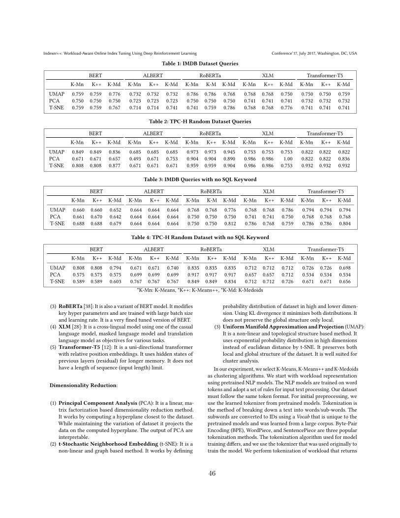
Indexer++: Workload-Aware Online Index Tuning Using Deep Reinforcement Learning Conference’17, July 2017, Washington, DC, USA

Table 1: IMDB Dataset Queries

BERTK-Mn K++ K-Md

UMAP 0.759 0.759 0.776PCA 0.750 0.750 0.750T-SNE 0.759 0.759 0.767

ALBERTK-Mn K++ K-Md0.732 0.732 0.7320.723 0.723 0.7230.714 0.714 0.741

RoBERTaK-Mn K-M K-Md0.786 0.786 0.7680.750 0.750 0.7500.741 0.759 0.786

XLMK-Mn K++ K-Md0.768 0.768 0.7500.741 0.741 0.7410.768 0.768 0.776

Transformer-T5K-Mn K++ K-Md0.750 0.750 0.7590.732 0.732 0.7320.741 0.741 0.741

Table 2: TPC-H Random Dataset Queries

BERTK-Mn K++ K-Md

UMAP 0.849 0.849 0.836PCA 0.671 0.671 0.657T-SNE 0.808 0.808 0.877

ALBERTK-Mn K++ K-Md0.685 0.685 0.6850.493 0.671 0.7530.671 0.671 0.671

RoBERTaK-Mn K++ K-Md0.973 0.973 0.9450.904 0.904 0.8900.959 0.959 0.904

XLMK-Mn K++ K-Md0.753 0.753 0.7530.986 0.986 1.000.986 0.986 0.753

Transformer-T5K-Mn K++ K-Md0.822 0.822 0.8220.822 0.822 0.8360.932 0.932 0.932

Table 3: IMDB Queries with no SQL Keyword

BERTK-Mn K++ K-Md

UMAP 0.660 0.660 0.652PCA 0.661 0.670 0.642T-SNE 0.688 0.688 0.679

ALBERTK-Mn K++ K-Md0.664 0.664 0.6640.664 0.664 0.6640.664 0.664 0.664

RoBERTaK-Mn K-M K-Md0.768 0.768 0.7760.750 0.750 0.7500.750 0.750 0.812

XLMK-Mn K++ K-Md0.768 0.768 0.7860.741 0.741 0.7500.786 0.768 0.759

Transformer-T5K-Mn K++ K-Md0.794 0.794 0.7940.768 0.768 0.7680.786 0.786 0.804

Table 4: TPC-H Random Dataset with no SQL Keyword

BERTK-Mn K++ K-Md

UMAP 0.808 0.808 0.794PCA 0.575 0.575 0.575T-SNE 0.589 0.589 0.603

ALBERTK-Mn K++ K-Md0.671 0.671 0.7400.699 0.699 0.6990.767 0.767 0.767

RoBERTaK-Mn K++ K-Md0.835 0.835 0.8350.917 0.917 0.9170.849 0.849 0.834

XLMK-Mn K++ K-Md0.712 0.712 0.7120.657 0.657 0.7120.712 0.712 0.726

Transformer-T5K-Mn K++ K-Md0.726 0.726 0.6980.534 0.534 0.5340.671 0.671 0.656

*K-Mn: K-Means, *K++: K-Means++, *K-Md: K-Medoids

(3) RoBERTa [38]: It is also a variant of BERTmodel. It modifieskey hyper parameters and are trained with large batch sizeand learning rate. It is a very fined tuned version of BERT.

(4) XLM [28]: It is a cross-lingual model using one of the casuallanguage model, masked language model and translationlanguage model as objectives for various tasks.

(5) Transformer-T5 [12]: It is a uni-directional transformerwith relative position embeddings. It uses hidden states ofprevious layers (residual) for longer memory. It does nothave a length of sequence (input length) limit.

Dimensionality Reduction:

(1) Principal Component Analysis (PCA): It is a linear, ma-trix factorization based dimensionality reduction method.It works by computing a hyperplane closest to the dataset.While maintaining the variation of dataset it projects thedata on the computed hyperplane. The output of PCA areinterpretable.

(2) t-Stochastic Neighborhood Embedding (t-SNE): It is anon-linear and graph based method. It works by defining

probability distribution of dataset in high and lower dimen-sion. Using KL divergence it minimizes both distributions. Itdoes not preserve the global structure only local.

(3) UniformManifoldApproximation andProjection (UMAP):It is a non-linear and topological structure based method. Ituses exponential probability distribution in high dimensionsinstead of euclidean distance by t-SNE. It preserves bothlocal and global structure of the dataset. It is well suited forcluster analysis.

In our experiment, we select K-Means, K-Means++ andK-Medoidsas clustering algorithms. We start with workload representationusing pretrained NLP models. The NLP models are trained on wordtokens and adopt a set of rules for input text processing. Our datasetmust follow the same token format. For initial preprocessing, weuse the learned tokenizer from pretrained models. Tokenization isthe method of breaking down a text into words/sub-words. Thesubwords are converted to IDs using a Vocab that is unique to thepretrained models and was learned from a large corpus. Byte-PairEncoding (BPE), WordPiece, and SentencePiece are three populartokenization methods. The tokenization algorithm used for modeltraining differs, and we use the tokenizer that was used originally totrain the model. We perform tokenization of workload that returns

46

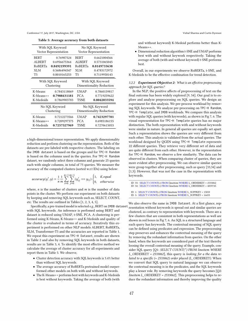
Conference’17, July 2017, Washington, DC, USA Vishal Sharma and Curtis Dyreson

Table 5: Average accuracy from both datasets

With SQL KeywordVector Representation

BERT 0.76987524ALBERT 0.6956675364RoBERTa 0.8492199391XLM 0.5686494347T5 0.8010165253

No SQL KeywordVector Representation

BERT 0.6621004566ALBERT 0.5731065045RoBERTa 0.8149733638XLM 0.4783172972T5 0.7119958143

With SQL KeywordClustering

K-Means 0.7843118069K-Means++ 0.7908431181K-Medoids 0.7869903783

With SQL KeywordDimentionality ReductionUMAP 0.7860159817PCA 0.7719259622TSNE 0.8042033594

No SQL KeywordClustering

K-Means 0.7212273566K-Means++ 0.7209297375K-Medoids 0.7257527969

No SQL KeywordDimentionality ReductionUMAP 0.7423297701PCA 0.6985186155TSNE 0.7270615053

a high-dimensional tensor representation. We apply dimensionalityreduction and perform clustering on the representation. Both of thedatasets are pre-labeled with respective clusters. The labeling onthe IMDB dataset is based on the groups and for TPC-H Randomis based on the columns used in the queries. For TPC-H Randomdataset, we randomly select three columns and generate 25 querieseach with single columns, in total of 75 queries. We measure theaccuracy of the computed clusters (sorted w.r.t IDs) using below:

𝑎𝑐𝑐𝑢𝑟𝑎𝑐𝑦 (𝑦′, 𝑦) = 1𝑛

1𝑚

𝑛−1∑𝑖=0

𝑚−1∑𝑗=0

(𝑦′𝑖 𝑗 == 𝑦𝑖 𝑗 ){1, if, 𝑒𝑞𝑢𝑎𝑙0, 𝑜𝑡ℎ𝑒𝑟𝑤𝑖𝑠𝑒

where, 𝑛 is the number of clusters and 𝑚 is the number of datapoints in the cluster. We perform our experiment on both datasetsby keeping and removing SQL keywords such as, SELECT, COUNT,etc. The results are outlined in Tables [1, 2, 3, 4, 5].

Specifically, a pre-trainedmodel is selected e.g.,BERT on IMDB datasetwith SQL keywords. An inference is perfomed using BERT anddataset is reduced using UMAP, t-SNE, PCA. A clustering is per-formed using K-Means, K-Means++ and K-Medoids and quality ofthe cluster is evaluated in terms of accuracy. Iteratively this ex-periment is performed on other NLP models ALBERT, RoBERTa,XLM, Transformer-T5 and the accuracies are reported in Table 1.We repeat this experiment on TPC-H Dataset, results are shownin Table 2 and also by removing SQL keywords in both datasets,results are in Table 3, 4. To identify the most effective method wecalculate the average of cluster accuracy for all experiments andreport them in Table 5. We observe,

• Cluster detection accuracy with SQL keywords is 3.4% betterthan without SQL keywords.

• The average accuracy of RoBERTa pretrained model ourper-formed other models on both with and without keywords.

• TheK-Means++ performs best with keywords andK-Medoidsis best without keywords. Taking the average of both (with

and without keyword) K-Medoid performs better than K-Means++.

• Dimensional reduction algorithm t-SNE and UMAP performsbest with and without keywork respectively. Taking theaverage of both (with and without keyword) t-SNE performsbest.

Overall, in our experiments we observe RoBERTa, t-SNE, andK-Medoids to be the effective combination for trend detection.

5.2.2 Experiment Objective 2: What is an effective preprocessingapproach for SQL queries?

In the NLP, the positive affects of preprocessing of text on thefinal outcome has been widely explored [9, 54]. Our goal is to ex-plore and analyze preprocessing on SQL queries. We design anexperiment for this analysis. We pre-process workload by remov-ing SQL keywords. We analyze pre-processing on TPC-H Random,TPC-H Template, and IMDB workloads. We compare this analysiswith regular SQL queries (with keywords), as shown in Fig 7, 6. Thevisual representation for TPC-H Template queries has no majordistinction. The both representation with and without keywordswere similar in nature. In general all queries are equally set apart.Such a representation shows the queries are very different fromeach other. This analysis is validated from the actual queries. Theworkload designed by QGEN using TPC-H Template represents22 different queries. They retrieve very different set of data andare quite different from each other. However, in the representationfor TPC-H Random, we observe a few similarity. The data can beobserved in clusters. When comparing cluster of queries, they aremore evident after preprocessing. We can observe similar querieswere group together after preprocessing, such as query [33,34] and[1,3]: However, that was not the case in the representation withkeywords.

ID 33: SELECT COUNT(∗) FROM lineitem WHERE L_ORDERKEY = 2533062ID 34: SELECT COUNT(∗) FROM lineitem WHERE L_ORDERKEY < 4839745

ID 1: SELECT COUNT(∗) FROM lineitem WHERE L_SUPPKEY < 15859ID 3: SELECT COUNT(∗) FROM lineitem WHERE L_SUPPKEY < 16455

We also observe the same in IMDB Dataset. At a first glance, rep-resentation without keywords is spread out and similar queries areclustered, as contrary to representation with keywords. There are afew clusters that are consistent in both representations as well areshown in red boxes in Fig 7, 6. An SQL is a structured language andeach query has keywords. The contextual meaning of SQL querycan be defined using predicates and expression. The preprocessingstep preserves and enhances the contextual meaning of the queryby removing the redundant information from queries. On the otherhand, when the keywords are considered part of the text therebyloosing the overall contextual meaning of the query. Example, con-sider SQL query [Q1: SELECT COUNT(*) FROM lineitem WHEREL_ORDERKEY = 2533062], this query is looking for a the data re-lated to a specific (= 2533062) order placed (L_ORDERKEY). Whenwe convert that SQL query to natural language we can observethe contextual meaning is in the predicates, and the SQL keywordsplay a lesser role. By removing keywords the query becomes [Q2:lineitem L_ORDERKEY = 2533062]. This preprocessing helps to re-duce the redundant information and thereby improving the quality

47

Indexer++: Workload-Aware Online Index Tuning Using Deep Reinforcement Learning Conference’17, July 2017, Washington, DC, USA

−100 0 100TPC-H TSNE feature space one

−150

−100

−50

0

50

100

150

TP

C-H

TS

NE

feat

ure

spac

etw

o

0

123

4

5 6

7

8

9

10

11

12

13

14

1516

17

18

19

20

21

−100 −50 0 50 100TPC-H Random TSNE feature one

−125

−100

−75

−50

−25

0

25

50

75

TP

C-H

Ran

dom

TS

NE

feat

ure

two

0

1

2

3 4

5

6

7

8

910 11

12 13

14

15

16

17

1819

20

2122

23

24

25

26

27

2829

3031

3233

34

3536

3738

39

4041

42

43

4445 46

47

48

49

50

51

5253

54

5556

57

58

59

60

61

62

6364

65

6667

68

69

70

7172

−5 0 5 10 15IMDB TSNE feature one

−4

−2

0

2

4

6

IMD

BT

SN

Efe

atu

retw

o

01

2

3 45 6

78910

111213

14151617

181920

2122

232425

2627

28 29

30 31323334

353637

383940

41

42

43

44

4546

47

4849

50

51

5253 5455

565758

596061

626364

65

6667

68

697071

7273

7475

76

777879

80

81

82

8384

85

868788

89

9091

929394

959697

9899100

101

102

103

104105106107108

109110111

Workload embeedded using RoBERTa

Figure 6: TPC-H Template, TPC-H Random, and IMDB workload representation. The numeric value represent serial number.

−100 −50 0 50TPC-H TSNE feature space one

−100

−50

0

50

100

TP

C-H

TS

NE

feat

ure

spac

etw

o

0

1

2

3

4

5

6

7

8

9

10

11

12

13

14

15

16

1718

19

20

21

−7 −6 −5 −4 −3TPC-H Random TSNE feature one

10

12

14

16

TP

C-H

Ran

dom

TS

NE

feat

ure

two

0

1

2

3

4

56

7

8

910

1112

13

14

15

1617

18

192021

22

2324

25

26

27

28

29

3031

323334

353637

38

3940

41

42

43

4445

4647

48

4950

51

52

53

54

55

56

57

5859

60

61

62

6364

65

6667

68

6970

71

72

0

1

2

3

4

56

7

8

910

1112

13

14

15

1617

18

192021

22

2324

25

26

27

28

29

3031

323334

353637

38

3940

41

42

43

4445

4647

48

4950

51

52

53

54

55

56

57

5859

60

61

62

6364

65

6667

68

6970

71

72

−7.5 −5.0 −2.5 0.0 2.5 5.0IMDB TSNE feature one

−7.5

−5.0

−2.5

0.0

2.5

5.0

7.5

IMD

BT

SN

Efe

atu

retw

o

01

2

3 45 6

7 8910

11

12

13

141516

1718

19

20

21

22

23

24

25

2627

28

2930

3132

3334353637

383940

414243

444546 4748

49

50515253

5455 565758

596061

626364

656667

68697071

7273

74

75

76

7778 7980

8182

83

84858687

8889

9091

929394959697

9899100101102103

104105

106

107108

109110111

SQL keywords are removed and workload embeedded using RoBERTa

Figure 7: TPC-H Template, TPC-H Random, and IMDBworkload representation with no keywords. The numeric value representserial number.of representation. With this observation we conclude that repre-sentation of SQL queries after preprocessing (removing keywords)is very effective.

5.2.3 Experiment Objective 3: Is our proposed DQN algorithmwith priority experience sweeping capable to learning the change inthe environment?

In this experiment, we aim to measure the online efficacy ofthe DQN algorithm for priority experience sweeping. To performsuch evaluation we design an experiment with IMDB Dataset andTPC-H Random dataset. In the modern software systems, applica-tions are regularly modified or added. Such modification changesthe workload. We simulate and evaluate our framework in such ascenarios as well. We introduce future Groups of queries by merg-ing and removing existing workloads. We categorize both datasetsin three groups as described earlier in section 5.1. Our generatedrandom queries from TPC-H consists of three groups, where Group1 consists of queries only on single column, Group 2 with exactlytwo columns and Group 3 with exactly three columns. A samplequeries from each group is shown below:

SELECT COUNT(∗) FROM LINEITEM WHERE L_PARTKEY = 30217SELECT COUNT(∗) FROM LINEITEM WHERE L_ORDERKEY < 4741856 AND

L_TAX = 0.02

SELECT COUNT(∗) FROM LINEITEM WHERE L_SUPPKEY > 16616 AND L_TAX< 0.06 AND L_PARTKEY > 82374

The cumulative rewards graph for both datasets are shown inFig 8 9 10 ??, where each experiment has 15,000 episodes and Group2 and 3 are introduced at 5,000 and 10,000 respectively.

In fig 8, we observe sharp decline in cumulative rewards atepisode 5,000 and 10,000 and progressive nature later. This ex-plains that the indexes chosen initially for Group 1 were not aseffective for Group 2. This result aligns with the dataset as all threegroups of IMDB dataset are entirely different from each other withno inter-dependency. However, in the TPC-H dataset groups havedependency on each other. This can be observed in Fig 9 10, whereboth Group 2 and 3 received a gain in performance from previousindexes. This experiment evaluates efficacy of our framework ontwo datasets in a few different scenarios.

6 CONCLUSION AND FUTUREWORKIn this paper, we propose Indexer++ a real-time solution for onlineindex selection using pretrained NLP models and Deep Reinforce-ment Learning. We describe our approach for a change in workloadpattern detection. We observe SQL representation to be effectiveusing t-SNE, K-Medoids and RoBERTa pretrained model. We also

48

Conference’17, July 2017, Washington, DC, USA Vishal Sharma and Curtis Dyreson

0 2500 5000 7500 10000 12500 15000Episodes

−1500

0

1500

3000

4500

Cu

mm

ula

tive

Rew

ard

s

Group 1 Group 2 Group 3

Episodic Rewards for IMDB at Group 1, Group 2, Group 3

Figure 8: CumulativeRewards byDQNagent on IMDBdataset.The dataset is introduced in three stages starting with Group1 as initial workload then Group 2 and 3.

0 2500 5000 7500 10000 12500 15000Episodes

01000200030004000

Cu

mm

ula

tive

Rew

ard

s

Group 1 Group 2 Group 3

Episodic Rewards for TPC-H at Groups (1), (2), (3)

Figure 9: Cumulative Rewards by DQN agent on TPC-Hdataset. The dataset is introduced in three stages startingwith Group 1 as initial workload then Group 2 and 3.

0 2500 5000 7500 10000 12500 15000Episodes

01500300045006000

Cu

mm

ula

tive

Rew

ard

s

Group 1 Group 1+2 Group 1+2+3

Episodic Rewards for TPC-H at Groups (1), (1+2), (1+2+3)

Figure 10: Cumulative Rewards by DQN agent on TPC-Hdataset. The dataset is introduced in three stages startingwith Group 1 as initial workload then combined with Group2 and 3.propose priority experience sweeping as an extension to DQN al-gorithm for generalization in an online environment. We evaluateour approach on three different datasets. In our experiments, weobserve our proposed framework is able to solve all the existingchallenges for an online index tuning namely, (1) Noise Resilience,(2) Overhead Cost, (3) Trend Detection Time, and (4) Response Timeand respond to changing workload patterns by selecting optimalset of indexes.

In the future, we plan to extent our workload pattern detection tobuild a classifier to predict runtime, cardinality estimate and error.We also plan to analyze the affect of SQL operator in workloadrepresentation.

REFERENCES[1] Joy Arulraj, Ran Xian, Lin Ma, and Andrew Pavlo. 2019. Predictive Indexing.

arXiv preprint arXiv:1901.07064 (2019).[2] Bortik Bandyopadhyay, Pranav Maneriker, Vedang Patel, Saumya Yashmohini

Sahai, Ping Zhang, and Srinivasan Parthasarathy. 2020. DrugDBEmbed: SemanticQueries on Relational Database using Supervised Column Encodings. arXivpreprint arXiv:2007.02384 (2020).

[3] Debabrota Basu, Qian Lin, Weidong Chen, Hoang Tam Vo, Zihong Yuan, PierreSenellart, and Stéphane Bressan. 2015. Cost-Model Oblivious Database Tuning

with Reinforcement Learning. In Proceedings, Part I, of the 26th InternationalConference on Database and Expert Systems Applications - Volume 9261 (Valencia,Spain) (DEXA 2015). Springer-Verlag, Berlin, Heidelberg, 253âĂŞ268. https://doi.org/10.1007/978-3-319-22849-5_18

[4] Yoshua Bengio, Aaron Courville, and Pascal Vincent. 2013. RepresentationLearning: A Review and New Perspectives. IEEE Trans. Pattern Anal. Mach. Intell.35, 8 (Aug. 2013), 1798–1828. https://doi.org/10.1109/TPAMI.2013.50

[5] Rajesh Bordawekar, Bortik Bandyopadhyay, and Oded Shmueli. 2017. Cognitivedatabase: A step towards endowing relational databases with artificial intelligencecapabilities. arXiv preprint arXiv:1712.07199 (2017).

[6] Rajesh Bordawekar and Oded Shmueli. 2017. Using word embedding to enablesemantic queries in relational databases. In Proceedings of the 1st Workshop onData Management for End-to-End Machine Learning. 1–4.

[7] N. Bruno and S. Chaudhuri. 2007. An Online Approach to Physical DesignTuning. In 2007 IEEE 23rd International Conference on Data Engineering. 826–835.https://doi.org/10.1109/ICDE.2007.367928

[8] N. Bruno and S. Chaudhuri. 2007. An Online Approach to Physical Design Tuning.In 2007 IEEE 23rd International Conference on Data Engineering. IEEE ComputerSociety, Los Alamitos, CA, USA, 826–835. https://doi.org/10.1109/ICDE.2007.367928

[9] Jose Camacho-Collados and Mohammad Taher Pilehvar. 2018. On the Role ofText Preprocessing in Neural Network Architectures: An Evaluation Study onText Categorization and Sentiment Analysis. In Proceedings of the 2018 EMNLPWorkshop BlackboxNLP: Analyzing and Interpreting Neural Networks for NLP.40–46.

[10] Riccardo Cappuzzo, Paolo Papotti, and Saravanan Thirumuruganathan. 2020.Creating Embeddings of Heterogeneous Relational Datasets for Data IntegrationTasks. In Proceedings of the 2020 ACM SIGMOD International Conference on Man-agement of Data (Portland, OR, USA) (SIGMOD ’20). Association for ComputingMachinery, New York, NY, USA, 1335âĂŞ1349. https://doi.org/10.1145/3318464.3389742

[11] Surajit Chaudhuri and Vivek R Narasayya. 1997. An efficient, cost-driven indexselection tool for Microsoft SQL server. In VLDB, Vol. 97. Citeseer, 146–155.

[12] Zihang Dai, Zhilin Yang, Yiming Yang, Jaime G Carbonell, Quoc Le, and RuslanSalakhutdinov. 2019. Transformer-XL: Attentive Language Models beyond aFixed-Length Context. In Proceedings of the 57th Annual Meeting of the Associationfor Computational Linguistics. 2978–2988.

[13] Sudipto Das, Miroslav Grbic, Igor Ilic, Isidora Jovandic, Andrija Jovanovic, Vivek RNarasayya, Miodrag Radulovic, Maja Stikic, Gaoxiang Xu, and Surajit Chaudhuri.2019. Automatically indexingmillions of databases inmicrosoft azure sql database.In Proceedings of the 2019 International Conference on Management of Data. 666–679.

[14] J. Devlin, Ming-Wei Chang, Kenton Lee, and Kristina Toutanova. 2019. BERT:Pre-training of Deep Bidirectional Transformers for Language Understanding. InNAACL-HLT.

[15] Bailu Ding, Sudipto Das, Ryan Marcus, Wentao Wu, Surajit Chaudhuri, andVivek R. Narasayya. 2019. AI Meets AI: Leveraging Query Executions to ImproveIndex Recommendations (SIGMOD ’19). Association for Computing Machinery,New York, NY, USA, 1241âĂŞ1258. https://doi.org/10.1145/3299869.3324957

[16] Martin R. Frank, Edward Omiecinski, and Shamkant B. Navathe. 1992. Adaptiveand Automated Index Selection in RDBMS. In Proceedings of the 3rd InternationalConference on Extending Database Technology: Advances in Database Technology(EDBT ’92). Springer-Verlag, Berlin, Heidelberg, 277âĂŞ292.

[17] Michael Günther. 2018. Freddy: Fast word embeddings in database systems. InProceedings of the 2018 International Conference on Management of Data. 1817–1819.

[18] Michael Hammer and Arvola Chan. 1976. Index selection in a self-adaptive database management system. In Proceedings of the 1976 ACM SIGMOD internationalconference on Management of data. 1–8.

[19] Michael Hammer and Arvola Chan. 1976. Index Selection in a Self-Adaptive DataBase Management System. In Proceedings of the 1976 ACM SIGMOD InternationalConference on Management of Data (Washington, D.C.) (SIGMOD ’76). Associationfor Computing Machinery, New York, NY, USA, 1âĂŞ8. https://doi.org/10.1145/509383.509385

[20] Matteo Hessel, Joseph Modayil, H. V. Hasselt, T. Schaul, Georg Ostrovski, W.Dabney, Dan Horgan, B. Piot, Mohammad Gheshlaghi Azar, and D. Silver. 2018.Rainbow: Combining Improvements in Deep Reinforcement Learning. ArXivabs/1710.02298 (2018).

[21] Geoffrey E Hinton et al. 1986. Learning distributed representations of concepts.In Proceedings of the eighth annual conference of the cognitive science society, Vol. 1.Amherst, MA, 12.

[22] Anil K Jain, M Narasimha Murty, and Patrick J Flynn. 1999. Data clustering: areview. ACM computing surveys (CSUR) 31, 3 (1999), 264–323.

[23] Shrainik Jain, Bill Howe, Jiaqi Yan, and Thierry Cruanes. 2018. Query2Vec: AnEvaluation of NLP Techniques for GeneralizedWorkload Analytics. arXiv preprintarXiv:1801.05613 (2018).

49

Indexer++: Workload-Aware Online Index Tuning Using Deep Reinforcement Learning Conference’17, July 2017, Washington, DC, USA

[24] Herald Kllapi, Ilia Pietri, Verena Kantere, and Yannis E Ioannidis. 2020. AutomatedManagement of Indexes for Dataflow Processing Engines in IaaS Clouds.. In EDBT.169–180.

[25] Piotr Kołaczkowski and Henryk Rybiński. 2009. Automatic Index Selection inRDBMS by Exploring Query Execution Plan Space. Springer Berlin Heidelberg,Berlin, Heidelberg, 3–24. https://doi.org/10.1007/978-3-642-02190-9_1

[26] J. Kossmann and R. Schlosser. 2019. A Framework for Self-Managing Data-base Systems. In 2019 IEEE 35th International Conference on Data EngineeringWorkshops (ICDEW). 100–106.

[27] Tim Kraska, Mohammad Alizadeh, Alex Beutel, H. Ed Chi, Ani Kristo, GuillaumeLeclerc, Samuel Madden, Hongzi Mao, and Vikram Nathan. 2019. SageDB - ALearned Database System. CIDR (2019).

[28] Guillaume Lample and Alexis Conneau. 2019. Cross-lingual language modelpretraining. arXiv preprint arXiv:1901.07291 (2019).

[29] Hai Lan, Zhifeng Bao, and Yuwei Peng. 2020. An Index Advisor Using DeepReinforcement Learning. In Proceedings of the 29th ACM International Conferenceon Information & Knowledge Management. 2105–2108.

[30] Zhenzhong Lan, Mingda Chen, Sebastian Goodman, Kevin Gimpel, PiyushSharma, and Radu Soricut. 2019. Albert: A lite bert for self-supervised learningof language representations. arXiv preprint arXiv:1909.11942 (2019).

[31] Quoc Le and Tomas Mikolov. 2014. Distributed representations of sentences anddocuments. In International conference on machine learning. PMLR, 1188–1196.

[32] Viktor Leis, Andrey Gubichev, Atanas Mirchev, Peter Boncz, Alfons Kemper, andThomas Neumann. 2015. How Good Are Query Optimizers, Really? Proc. VLDBEndow. 9, 3 (Nov. 2015), 204–215. https://doi.org/10.14778/2850583.2850594

[33] Omer Levy and Yoav Goldberg. 2014. Linguistic regularities in sparse and explicitword representations. In Proceedings of the eighteenth conference on computationalnatural language learning. 171–180.

[34] Omer Levy and Yoav Goldberg. 2014. Linguistic regularities in sparse and explicitword representations. In Proceedings of the eighteenth conference on computationalnatural language learning. 171–180.

[35] J. Lilleberg, Y. Zhu, and Y. Zhang. 2015. Support vector machines and Word2vecfor text classification with semantic features. In 2015 IEEE 14th InternationalConference on Cognitive Informatics Cognitive Computing (ICCI*CC). 136–140.https://doi.org/10.1109/ICCI-CC.2015.7259377

[36] Zhouhan Lin, Minwei Feng, Cicero Nogueira dos Santos, Mo Yu, Bing Xiang,Bowen Zhou, and Yoshua Bengio. 2017. A structured self-attentive sentenceembedding. arXiv preprint arXiv:1703.03130 (2017).

[37] Pengfei Liu, Xipeng Qiu, and Xuanjing Huang. 2016. Recurrent neural networkfor text classification with multi-task learning. In Proceedings of the Twenty-FifthInternational Joint Conference on Artificial Intelligence. 2873–2879.

[38] Yinhan Liu, Myle Ott, Naman Goyal, Jingfei Du, Mandar Joshi, Danqi Chen, OmerLevy, Mike Lewis, Luke Zettlemoyer, and Veselin Stoyanov. 2019. RoBERTa: ARobustly Optimized BERT Pretraining Approach. CoRR abs/1907.11692 (2019).arXiv:1907.11692 http://arxiv.org/abs/1907.11692

[39] M. Luhring, K. Sattler, K. Schmidt, and E. Schallehn. 2007. Autonomous Man-agement of Soft Indexes. In 2007 IEEE 23rd International Conference on DataEngineering Workshop. 450–458. https://doi.org/10.1109/ICDEW.2007.4401028

[40] Mingbo Ma, Liang Huang, Bowen Zhou, and Bing Xiang. 2015. Dependency-based Convolutional Neural Networks for Sentence Embedding. In Proceedingsof the 53rd Annual Meeting of the Association for Computational Linguistics andthe 7th International Joint Conference on Natural Language Processing (Volume 2:Short Papers). 174–179.

[41] Qiang Ma, Suwen Ge, Danyang He, Darshan Thaker, and Iddo Drori. 2019. Com-binatorial Optimization by Graph Pointer Networks and Hierarchical Reinforce-ment Learning. arXiv:1911.04936 [cs.LG]

[42] Tomas Mikolov, Kai Chen, G. S. Corrado, and J. Dean. 2013. Efficient Estimationof Word Representations in Vector Space. In ICLR.

[43] Mohammadreza Nazari, Afshin Oroojlooy, Lawrence Snyder, and Martin Takác.2018. Reinforcement learning for solving the vehicle routing problem. InAdvancesin Neural Information Processing Systems. 9839–9849.

[44] Priscilla Neuhaus, Julia Couto, Jonatas Wehrmann, Duncan Dubugras AlcobaRuiz, and Felipe Rech Meneguzzi. 2019. GADIS: A genetic algorithm for databaseindex selection. In The 31st International Conference on Software Engineering &Knowledge Engineering, 2019, Portugal.

[45] Andrew Pavlo, Gustavo Angulo, Joy Arulraj, Haibin Lin, Jiexi Lin, Lin Ma,Prashanth Menon, Todd C Mowry, Matthew Perron, Ian Quah, et al. 2017. Self-Driving Database Management Systems.. In CIDR, Vol. 4. 1.

[46] Wendel Góes Pedrozo, Júlio Cesar Nievola, and Deborah Carvalho Ribeiro. 2018.An Adaptive Approach for Index Tuning with Learning Classifier Systems onHybrid Storage Environments. In Hybrid Artificial Intelligent Systems, Fran-cisco Javier de Cos Juez, José Ramón Villar, Enrique A. de la Cal, Álvaro Herrero,Héctor Quintián, José António Sáez, and Emilio Corchado (Eds.). Springer Inter-national Publishing, Cham, 716–729.

[47] Gregory Piatetsky-Shapiro. 1983. The Optimal Selection of Secondary Indices isNP-Complete. SIGMOD Rec. 13, 2 (Jan. 1983), 72âĂŞ75.

[48] Z. Sadri, L. Gruenwald, and E. Leal. 2020. Online Index Selection Using DeepReinforcement Learning for a Cluster Database. In 2020 IEEE 36th InternationalConference on Data Engineering Workshops (ICDEW). 158–161. https://doi.org/10.1109/ICDEW49219.2020.00035

[49] Zahra Sadri, Le Gruenwald, and Eleazar Leal. 2020. Online Index SelectionUsing Deep Reinforcement Learning for a Cluster Database. In 2020 IEEE 36thInternational Conference on Data Engineering Workshops (ICDEW). IEEE, 158–161.

[50] Karl Schnaitter, Serge Abiteboul, Tova Milo, and Neoklis Polyzotis. 2006. Colt:continuous on-line tuning. In Proceedings of the 2006 ACM SIGMOD internationalconference on Management of data. 793–795.

[51] Karl Schnaitter, Neoklis Polyzotis, and Lise Getoor. 2009. Index Interactionsin Physical Design Tuning: Modeling, Analysis, and Applications. Proc. VLDBEndow. 2, 1 (Aug. 2009), 1234âĂŞ1245. https://doi.org/10.14778/1687627.1687766

[52] Aliaksei Severyn and Alessandro Moschitti. 2015. Twitter Sentiment Analysiswith Deep Convolutional Neural Networks. In Proceedings of the 38th InternationalACM SIGIR Conference on Research and Development in Information Retrieval(Santiago, Chile) (SIGIR ’15). Association for Computing Machinery, New York,NY, USA, 959âĂŞ962. https://doi.org/10.1145/2766462.2767830

[53] Ankur Sharma, Felix Martin Schuhknecht, and Jens Dittrich. 2018. The Case forAutomatic Database Administration using Deep Reinforcement Learning. CoRRabs/1801.05643 (2018). arXiv:1801.05643 http://arxiv.org/abs/1801.05643

[54] Xiaobing Sun, Xiangyue Liu, Jiajun Hu, and Junwu Zhu. 2014. Empirical Studieson the NLP Techniques for Source Code Data Preprocessing. In Proceedings of the2014 3rd International Workshop on Evidential Assessment of Software Technologies(Nanjing, China) (EAST 2014). Association for Computing Machinery, New York,NY, USA, 32âĂŞ39. https://doi.org/10.1145/2627508.2627514

[55] Richard S Sutton and Andrew G Barto. 2018. Reinforcement learning: An intro-duction. MIT press.

[56] Richard S Sutton and Andrew G Barto. 2018. Reinforcement learning: An intro-duction. MIT press.

[57] Gary Valentin, Michael Zuliani, Daniel C Zilio, Guy Lohman, and Alan Skelley.2000. DB2 advisor: An optimizer smart enough to recommend its own indexes.In Proceedings of 16th International Conference on Data Engineering (Cat. no.00CB37073). IEEE, 101–110.

[58] Dana Van Aken, Andrew Pavlo, Geoffrey J. Gordon, and Bohan Zhang. 2017.Automatic Database Management System Tuning Through Large-Scale MachineLearning. In Proceedings of the 2017 ACM International Conference on Managementof Data (Chicago, Illinois, USA) (SIGMOD ’17). Association for ComputingMachin-ery, New York, NY, USA, 1009âĂŞ1024. https://doi.org/10.1145/3035918.3064029

[59] Zhengtong Yan, Jiaheng Lu, Naresh Chainani, and Chunbin Lin. [n.d.]. Workload-Aware Performance Tuning for Autonomous DBMSs. Machine learning 13 ([n. d.]),15.

[60] Shengyu Zhu, Ignavier Ng, and Zhitang Chen. 2020. Causal Discovery withReinforcement Learning. In International Conference on Learning Representations(ICLR).

50

51

CHAPTER 5

Conclusion and Future Work

A Self Managing Database eliminates the burden of managing and performing self-

tuning of its parameters. They provide the most efficient way to store and retrieve data.

In a step towards such databases we proposed and evaluate our frameworks MANTIS and

Indexer++ that are able to tune configurations by itself and also provide assistance to

users by recommending indexes in real-time. Analyzing large data and millions of queries

can be a challenging task. A Database Assistant can help us identify ‘interesting’ queries

in a large corpus of queries, recommend sets of queries, and summarize a workload. We

propose and evaluate Query Enhancer a contextual SQL query enhancer able to recommend

interesting queries. To understand and link the relationship of tables in a database we

propose LinkSocial. We perform extensive evaluations of our frameworks using multiple

datasets and compare our results with existing state-of-the-art approaches. Our proposed

frameworks out performs existing approaches.

In future, we plan to extent our work in a few ways. An exciting area of future research

is to extent our workload pattern detection to predict run time, cardinality estimate and

error from workload. Another area of exploration is to optimize several database parameters

using reinforcement learning and eventually leading towards an autonomous self managing

database. Our proposed Query Enhancer can be a extended as a platform for learning SQL,

and this framework will be independent of platforms and can perform equally well across-

platform. Entity Resolution on social media can be extended to study a user’s behavior

across platforms. To our knowledge such an analysis has not yet been studied.

52

REFERENCES

[1] J. Tan, T. Zhang, F. Li, J. Chen, Q. Zheng, P. Zhang, H. Qiao, Y. Shi, W. Cao,

and R. Zhang, “Ibtune: Individualized buffer tuning for large-scale cloud databases,”

Proc. VLDB Endow., vol. 12, no. 10, p. 1221–1234, Jun. 2019. [Online]. Available:

https://doi.org/10.14778/3339490.3339503

[2] T. Kraska, A. Beutel, E. H. Chi, J. Dean, and N. Polyzotis, “The case for learned index

structures,” in Proceedings of the 2018 International Conference on Management of

Data, ser. SIGMOD ’18. New York, NY, USA: Association for Computing Machinery,

2018, p. 489–504. [Online]. Available: https://doi.org/10.1145/3183713.3196909

[3] B. Hilprecht, C. Binnig, and U. Rohm, “Towards learning a partitioning advisor with

deep reinforcement learning,” in Proceedings of the Second International Workshop

on Exploiting Artificial Intelligence Techniques for Data Management, ser. aiDM ’19.

New York, NY, USA: Association for Computing Machinery, 2019. [Online]. Available:

https://doi.org/10.1145/3329859.3329876

[4] R. Marcus and O. Papaemmanouil, “Deep reinforcement learning for join

order enumeration,” in Proceedings of the First International Workshop on

Exploiting Artificial Intelligence Techniques for Data Management, ser. aiDM’18.

New York, NY, USA: ACM, 2018, pp. 3:1–3:4. [Online]. Available: http:

//doi.acm.org/10.1145/3211954.3211957

[5] X. Zhou, C. Chai, G. Li, and J. SUN, “Database meets artificial intelligence: A survey,”

IEEE Transactions on Knowledge Data Engineering, no. 01, pp. 1–1, may 5555.

53

[6] S. Agrawal, S. Chaudhuri, L. Kollar, A. Marathe, V. Narasayya, and M. Syamala,

“Database tuning advisor for microsoft sql server 2005,” in Proceedings of the 2005

ACM SIGMOD international conference on Management of data, 2005, pp. 930–932.

[7] M. Hammer, “Self-adaptive automatic data base design,” in Proceedings of the June

13-16, 1977, national computer conference, 1977, pp. 123–129.

[8] M. Hammer and A. Chan, “Index selection in a self-adaptive data base management

system,” in Proceedings of the 1976 ACM SIGMOD international conference on Man-

agement of data, 1976, pp. 1–8.

[9] M. Hammer and B. Niamir, “A heuristic approach to attribute partitioning,” in Pro-

ceedings of the 1979 ACM SIGMOD international conference on Management of data,

1979, pp. 93–101.

[10] M. Frank, E. Omiecinski, and S. Navathe, “Adaptive and automative index selection

in rdbms,” in Proceedings of EDBT, vol. 92.

[11] G. Weikum, C. Hasse, A. Monkeberg, and P. Zabback, “The comfort automatic tuning

project,” Information systems, vol. 19, no. 5, pp. 381–432, 1994.

[12] S. Chaudhuri and V. R. Narasayya, “An efficient, cost-driven index selection tool for

microsoft sql server,” in VLDB, vol. 97. Citeseer, 1997, pp. 146–155.

[13] S. Chaudhuri and V. Narasayya, “Physical database design assistant and wizard for

sql server,” Microsoft Research Technical report, in preparation, Tech. Rep., 1997.

[14] G. Weikum, A. Moenkeberg, C. Hasse, and P. Zabback, “Self-tuning database tech-

nology and information services: from wishful thinking to viable engineering,” in

VLDB’02: Proceedings of the 28th International Conference on Very Large Databases.

Elsevier, 2002, pp. 20–31.

[15] W. Tian, P. Martin, and W. Powley, “Techniques for automatically sizing multiple

buffer pools in db2,” in Proceedings of the 2003 conference of the Centre for Advanced

Studies on Collaborative research, 2003, pp. 294–302.

54

[16] G. Valentin, M. Zuliani, D. C. Zilio, G. Lohman, and A. Skelley, “Db2 advisor: An

optimizer smart enough to recommend its own indexes,” in Proceedings of 16th Inter-

national Conference on Data Engineering (Cat. no. 00CB37073). IEEE, 2000, pp.

101–110.

[17] D. C. Zilio, J. Rao, S. Lightstone, G. Lohman, A. Storm, C. Garcia-Arellano, and

S. Fadden, “Db2 design advisor: integrated automatic physical database design,” in

Proceedings of the Thirtieth international conference on Very large data bases-Volume

30, 2004, pp. 1087–1097.

[18] A. J. Storm, C. Garcia-Arellano, S. S. Lightstone, Y. Diao, and M. Surendra, “Adaptive

self-tuning memory in db2,” in Proceedings of the 32nd international conference on

Very large data bases, 2006, pp. 1081–1092.

[19] B. Dageville and M. Zait, “Sql memory management in oracle9i,” in VLDB’02: Pro-

ceedings of the 28th International Conference on Very Large Databases. Elsevier, 2002,

pp. 962–973.

[20] B. Dageville and K. Dias, “Oracle’s self-tuning architecture and solutions.”

[21] A. Pavlo, M. Butrovich, A. Joshi, L. Ma, P. Menon, D. V. Aken, L. J. Lee, and

R. Salakhutdinov, “External vs. internal: An essay on machine learning agents for

autonomous database management systems,” IEEE Data Eng. Bull., vol. 42, pp. 32–

46, 2019.

[22] D. Van Aken, A. Pavlo, G. J. Gordon, and B. Zhang, “Automatic database

management system tuning through large-scale machine learning,” in Proceedings of

the 2017 ACM International Conference on Management of Data, ser. SIGMOD ’17.

New York, NY, USA: Association for Computing Machinery, 2017, p. 1009–1024.

[Online]. Available: https://doi.org/10.1145/3035918.3064029

[23] B. Zhang, D. Van Aken, J. Wang, T. Dai, S. Jiang, J. Lao, S. Sheng, A. Pavlo, and

G. J. Gordon, “A demonstration of the ottertune automatic database management

55

system tuning service,” Proc. VLDB Endow., vol. 11, no. 12, p. 1910–1913, Aug. 2018.

[Online]. Available: https://doi.org/10.14778/3229863.3236222

[24] T. Kraska, M. Alizadeh, A. Beutel, H. E. Chi, A. Kristo, G. Leclerc, S. Madden,

H. Mao, and V. Nathan, “Sagedb - a learned database system,” CIDR, 2019.

[25] J. Kossmann and R. Schlosser, “A framework for self-managing database systems,” in

2019 IEEE 35th International Conference on Data Engineering Workshops (ICDEW),

2019, pp. 100–106.

[26] A. Pavlo, G. Angulo, J. Arulraj, H. Lin, J. Lin, L. Ma, P. Menon, T. C. Mowry,

M. Perron, I. Quah et al., “Self-driving database management systems,” vol. 4, 2017,

p. 1.

[27] B. Ding, S. Das, R. Marcus, W. Wu, S. Chaudhuri, and V. R. Narasayya, “Ai meets

ai: Leveraging query executions to improve index recommendations,” ser. SIGMOD

’19. New York, NY, USA: Association for Computing Machinery, 2019, p. 1241–1258.

[Online]. Available: https://doi.org/10.1145/3299869.3324957

[28] P. Neuhaus, J. Couto, J. Wehrmann, D. D. A. Ruiz, and F. R. Meneguzzi, “Gadis: A

genetic algorithm for database index selection,” in The 31st International Conference

on Software Engineering & Knowledge Engineering, 2019, Portugal., 2019.

[29] X. Yu, G. Li, C. Chai, and N. Tang, “Reinforcement learning with tree-lstm for join

order selection,” in 2020 IEEE 36th International Conference on Data Engineering

(ICDE), 2020, pp. 1297–1308.

[30] I. Trummer, S. Moseley, D. Maram, S. Jo, and J. Antonakakis, “Skinnerdb:

Regret-bounded query evaluation via reinforcement learning,” Proc. VLDB

Endow., vol. 11, no. 12, pp. 2074–2077, Aug. 2018. [Online]. Available:

https://doi.org/10.14778/3229863.3236263

56

[31] R. Marcus and O. Papaemmanouil, “Towards a hands-free query optimizer

through deep learning,” CoRR, vol. abs/1809.10212, 2018. [Online]. Available:

http://arxiv.org/abs/1809.10212

[32] S. Krishnan, Z. Yang, K. Goldberg, J. M. Hellerstein, and I. Stoica, “Learning to

optimize join queries with deep reinforcement learning,” CoRR, vol. abs/1808.03196,

2018. [Online]. Available: http://arxiv.org/abs/1808.03196

[33] J. Ortiz, M. Balazinska, J. Gehrke, and S. S. Keerthi, “Learning state representations

for query optimization with deep reinforcement learning,” in Proceedings of the Second

Workshop on Data Management for End-To-End Machine Learning, 2018, pp. 1–4.

[34] S. Krishnan, Z. Yang, K. Goldberg, J. Hellerstein, and I. Stoica, “Learning to optimize

join queries with deep reinforcement learning,” 2018.

[35] J. Zhang, Y. Liu, K. Zhou, G. Li, Z. Xiao, B. Cheng, J. Xing, Y. Wang,

T. Cheng, L. Liu, M. Ran, and Z. Li, “An end-to-end automatic cloud database

tuning system using deep reinforcement learning,” in Proceedings of the 2019

International Conference on Management of Data, ser. SIGMOD ’19. New York, NY,

USA: Association for Computing Machinery, 2019, p. 415–432. [Online]. Available:

https://doi.org/10.1145/3299869.3300085

[36] G. Li, X. Zhou, S. Li, and B. Gao, “Qtune: A query-aware database tuning system

with deep reinforcement learning,” Proc. VLDB Endow., vol. 12, no. 12, p. 2118–2130,

Aug. 2019. [Online]. Available: https://doi.org/10.14778/3352063.3352129

[37] G. C. Durand, M. Pinnecke, R. Piriyev, M. Mohsen, D. Broneske, G. Saake, M. S.

Sekeran, F. Rodriguez, and L. Balami, “Gridformation: Towards self-driven online

data partitioning using reinforcement learning,” in aiDM’18, 2018.

[38] Z. Yang, B. Chandramouli, C. Wang, J. Gehrke, Y. Li, U. F. Minhas, P.-r.

Larson, D. Kossmann, and R. Acharya, “Qd-tree: Learning data layouts for

big data analytics,” in Proceedings of the 2020 ACM SIGMOD International

57

Conference on Management of Data, ser. SIGMOD ’20. New York, NY, USA:

Association for Computing Machinery, 2020, p. 193–208. [Online]. Available:

https://doi.org/10.1145/3318464.3389770

[39] D. Basu, Q. Lin, W. Chen, H. T. Vo, Z. Yuan, P. Senellart, and S. Bressan,

“Cost-model oblivious database tuning with reinforcement learning,” in Proceedings,

Part I, of the 26th International Conference on Database and Expert Systems

Applications - Volume 9261, ser. DEXA 2015. Berlin, Heidelberg: Springer-Verlag,

2015, p. 253–268. [Online]. Available: https://doi.org/10.1007/978-3-319-22849-5 18

[40] A. Sharma, F. M. Schuhknecht, and J. Dittrich, “The case for automatic database

administration using deep reinforcement learning,” CoRR, vol. abs/1801.05643, 2018.

[Online]. Available: http://arxiv.org/abs/1801.05643

[41] J. Welborn, M. Schaarschmidt, and E. Yoneki, “Learning index selection with struc-

tured action spaces,” arXiv preprint arXiv:1909.07440, 2019.

[42] G. P. Licks, J. C. Couto, P. de Fatima Miehe, R. De Paris, D. D. Ruiz, and

F. Meneguzzi, “Smartix: A database indexing agent based on reinforcement learning,”

Applied Intelligence, pp. 1–14, 2020.

[43] H. Kllapi, I. Pietri, V. Kantere, and Y. E. Ioannidis, “Automated management of

indexes for dataflow processing engines in iaas clouds.” in EDBT, 2020, pp. 169–180.

[44] M. Luhring, K. Sattler, K. Schmidt, and E. Schallehn, “Autonomous management

of soft indexes,” in 2007 IEEE 23rd International Conference on Data Engineering

Workshop, 2007, pp. 450–458.

[45] K. Schnaitter, S. Abiteboul, T. Milo, and N. Polyzotis, “Colt: Continuous

on-line tuning,” in Proceedings of the 2006 ACM SIGMOD International

Conference on Management of Data, ser. SIGMOD ’06. New York, NY, USA:

Association for Computing Machinery, 2006, p. 793–795. [Online]. Available:

https://doi.org/10.1145/1142473.1142592

58

[46] W. G. Pedrozo, J. C. Nievola, and D. C. Ribeiro, “An adaptive approach for index

tuning with learning classifier systems on hybrid storage environments,” in Hybrid

Artificial Intelligent Systems, F. J. de Cos Juez, J. R. Villar, E. A. de la Cal, A. Her-

rero, H. Quintian, J. A. Saez, and E. Corchado, Eds. Cham: Springer International

Publishing, 2018, pp. 716–729.

[47] S. Das, M. Grbic, I. Ilic, I. Jovandic, A. Jovanovic, V. R. Narasayya, M. Radulovic,

M. Stikic, G. Xu, and S. Chaudhuri, “Automatically indexing millions of

databases in microsoft azure sql database,” in Proceedings of the 2019 International

Conference on Management of Data, ser. SIGMOD ’19. New York, NY, USA:

Association for Computing Machinery, 2019, p. 666–679. [Online]. Available:

https://doi.org/10.1145/3299869.3314035

[48] Z. Sadri, L. Gruenwald, and E. Leal, “Online index selection using deep reinforcement

learning for a cluster database,” in 2020 IEEE 36th International Conference on Data

Engineering Workshops (ICDEW), 2020, pp. 158–161.

[49] J. Zhang, Y. Liu, K. Zhou, G. Li, Z. Xiao, B. Cheng, J. Xing, Y. Wang,

T. Cheng, L. Liu, M. Ran, and Z. Li, “An end-to-end automatic cloud database

tuning system using deep reinforcement learning,” in Proceedings of the 2019

International Conference on Management of Data, ser. SIGMOD ’19. New York, NY,

USA: Association for Computing Machinery, 2019, p. 415–432. [Online]. Available:

https://doi.org/10.1145/3299869.3300085

[50] M. Olma, M. Karpathiotakis, I. Alagiannis, M. Athanassoulis, and A. Ailamaki,

“Slalom: Coasting through raw data via adaptive partitioning and indexing,” Proc.

VLDB Endow., vol. 10, no. 10, p. 1106–1117, Jun. 2017. [Online]. Available:

https://doi.org/10.14778/3115404.3115415

[51] S. Chaudhuri, A. K. Gupta, and V. Narasayya, “Compressing sql workloads,” in Pro-

ceedings of the 2002 ACM SIGMOD international conference on Management of data,

2002, pp. 488–499.

59

[52] P. Ko laczkowski, “Compressing very large database workloads for continuous online

index selection,” in International Conference on Database and Expert Systems Appli-

cations. Springer, 2008, pp. 791–799.

[53] B. Babcock, S. Chaudhuri, and G. Das, “Dynamic sample selection for approximate

query processing,” in Proceedings of the 2003 ACM SIGMOD International

Conference on Management of Data, ser. SIGMOD ’03. New York, NY, USA:

Association for Computing Machinery, 2003, p. 539–550. [Online]. Available:

https://doi.org/10.1145/872757.872822

[54] S. Jain, B. Howe, J. Yan, and T. Cruanes, “Query2vec: An evaluation of nlp techniques

for generalized workload analytics,” arXiv preprint arXiv:1801.05613, 2018.

[55] V. Zhong, C. Xiong, and R. Socher, “Seq2sql: Generating structured queries from

natural language using reinforcement learning,” arXiv preprint arXiv:1709.00103, 2017.

[56] P. Wang, T. Shi, and C. K. Reddy, “Text-to-sql generation for question answering on

electronic medical records,” in Proceedings of The Web Conference 2020, 2020, pp.

350–361.

[57] S. E. Whang, D. Marmaros, and H. Garcia-Molina, “Pay-as-you-go entity resolution,”

IEEE Transactions on Knowledge and Data Engineering, vol. 25, no. 5, pp. 1111–1124,

2012.

[58] J. Cai and M. Strube, “End-to-end coreference resolution via hypergraph partitioning,”

in Proceedings of the 23rd International Conference on Computational Linguistics (Col-

ing 2010), 2010, pp. 143–151.

[59] Y. Qian, Y. Hu, J. Cui, Q. Zheng, and Z. Nie, “Combining machine learning and human

judgment in author disambiguation,” in Proceedings of the 20th ACM international

conference on Information and knowledge management, 2011, pp. 1241–1246.

60

[60] K. Shu, S. Wang, J. Tang, R. Zafarani, and H. Liu, “User identity linkage across online

social networks: A review,” Acm Sigkdd Explorations Newsletter, vol. 18, no. 2, pp.

5–17, 2017.

[61] S. Liu, S. Wang, F. Zhu, J. Zhang, and R. Krishnan, “Hydra: Large-scale social

identity linkage via heterogeneous behavior modeling,” in Proceedings of the 2014 ACM

SIGMOD international conference on Management of data, 2014, pp. 51–62.

[62] H. Zhang, M.-Y. Kan, Y. Liu, and S. Ma, “Online social network profile linkage,” in

Asia Information Retrieval Symposium. Springer, 2014, pp. 197–208.

[63] W. W. Cohen and J. Richman, “Learning to match and cluster large high-dimensional

data sets for data integration,” in Proceedings of the eighth ACM SIGKDD interna-

tional conference on Knowledge discovery and data mining, 2002, pp. 475–480.

[64] P. Jain, P. Kumaraguru, and A. Joshi, “@ i seek’fb. me’ identifying users across multiple

online social networks,” in Proceedings of the 22nd international conference on World

Wide Web, 2013, pp. 1259–1268.

[65] Y. Li, Z. Zhang, Y. Peng, H. Yin, and Q. Xu, “Matching user accounts based on

user generated content across social networks,” Future Generation Computer Systems,

vol. 83, pp. 104–115, 2018.

[66] A. Nunes, P. Calado, and B. Martins, “Resolving user identities over social networks

through supervised learning and rich similarity features,” in Proceedings of the 27th

Annual ACM symposium on applied computing, 2012, pp. 728–729.

[67] J. Liu, F. Zhang, X. Song, Y.-I. Song, C.-Y. Lin, and H.-W. Hon, “What’s in a name?

an unsupervised approach to link users across communities,” in Proceedings of the sixth

ACM international conference on Web search and data mining, 2013, pp. 495–504.

[68] R. Zafarani and H. Liu, “Connecting corresponding identities across communities.”

ICWSM, vol. 9, pp. 354–357, 2009.

61

[69] Q. Ma, H. H. Song, S. Muthukrishnan, and A. Nucci, “Joining user profiles across online

social networks: From the perspective of an adversary,” in 2016 IEEE/ACM Interna-

tional Conference on Advances in Social Networks Analysis and Mining (ASONAM).

IEEE, 2016, pp. 178–185.

[70] R. Zafarani and H. Liu, “Connecting users across social media sites: a behavioral-

modeling approach,” in Proceedings of the 19th ACM SIGKDD international conference

on Knowledge discovery and data mining, 2013, pp. 41–49.

[71] X. Mu, F. Zhu, E.-P. Lim, J. Xiao, J. Wang, and Z.-H. Zhou, “User identity linkage by

latent user space modelling,” in Proceedings of the 22nd ACM SIGKDD International

Conference on Knowledge Discovery and Data Mining, 2016, pp. 1775–1784.

[72] G. Silvestri, J. Yang, A. Bozzon, and A. Tagarelli, “Linking accounts across social

networks: the case of stackoverflow, github and twitter.” in KDWeb, 2015, pp. 41–52.

[73] G. Quercini, N. Bennacer, M. Ghufran, and C. N. Jipmo, “Liaison: reconciliation of

individuals profiles across social networks,” in Advances in Knowledge Discovery and

Management. Springer, 2017, pp. 229–253.