Amenity-Based Housing Affordability Indexes
42
2009 V37 4: pp. 705–746 REAL ESTATE ECONOMICS Amenity-Based Housing Affordability Indexes Lynn M. Fisher, ∗ Henry O. Pollakowski ∗∗ and Jeffrey Zabel ∗∗∗ The recent slump notwithstanding, substantial increases in house prices in many parts of the United States have served to highlight housing affordability for moderate-income households, especially in high-cost, supply-constrained coastal cities such as Boston. In this article, we develop a new measure of area affordability that characterizes the supply of housing that is affordable to different households in different locations of a metropolitan region. Key to our approach is the explicit recognition that the price/rent of a dwelling is affected by its location. Hence, we develop an affordability methodology that accounts for job accessibility, school quality and safety. This allows us to produce a menu of town-level indexes of adjusted housing affordability. The adjustments are based on obtaining implicit prices of these amenities from a hedonic price equation. We thus use data from a wide variety of sources to rank 141 towns in the greater Boston metropolitan area based on their adjusted affordability. Taking households earning 80% of area median income as an example, we find that consideration of town-level amenities leads to major changes relative to a typical assessment of affordability. The recent substantial increases in house prices in many parts of the United States have served to highlight housing affordability issues for moderate in- come households, especially in high-cost coastal cities, such as Boston, Mas- sachusetts (Goodman and Rodda 2005). During the period 1998–2005, house prices in the Boston metropolitan area nearly doubled. For a variety of reasons, average housing prices in such cities are unlikely to dramatically decline (even considering the recent slump). These high housing prices are particularly rele- vant to potential new entrants and other marginal households deciding whether to stay or leave. Many workers may choose not to locate in places such as Boston, even when their economic contribution to the area would have been positive. ∗ Department of Urban Studies and Planning, Center for Real Estate, Massachusetts Institute of Technology, Boston, MA 02139 or lfi[email protected]. ∗∗ Center for Real Estate, Massachusetts Institute of Technology, Boston, MA 02139 or [email protected]. ∗∗∗ Economics Department, Tufts University, Medford, MA 02155 or jeff.zabel@tufts. edu. C 2009 American Real Estate and Urban Economics Association
Transcript of Amenity-Based Housing Affordability Indexes

2009 V37 4: pp. 705–746
REAL ESTATE
ECONOMICS
Amenity-Based Housing AffordabilityIndexesLynn M. Fisher,∗ Henry O. Pollakowski∗∗ and Jeffrey Zabel∗∗∗
The recent slump notwithstanding, substantial increases in house prices inmany parts of the United States have served to highlight housing affordabilityfor moderate-income households, especially in high-cost, supply-constrainedcoastal cities such as Boston. In this article, we develop a new measure ofarea affordability that characterizes the supply of housing that is affordable todifferent households in different locations of a metropolitan region. Key to ourapproach is the explicit recognition that the price/rent of a dwelling is affectedby its location. Hence, we develop an affordability methodology that accountsfor job accessibility, school quality and safety. This allows us to produce amenu of town-level indexes of adjusted housing affordability. The adjustmentsare based on obtaining implicit prices of these amenities from a hedonic priceequation. We thus use data from a wide variety of sources to rank 141 townsin the greater Boston metropolitan area based on their adjusted affordability.Taking households earning 80% of area median income as an example, wefind that consideration of town-level amenities leads to major changes relativeto a typical assessment of affordability.
The recent substantial increases in house prices in many parts of the UnitedStates have served to highlight housing affordability issues for moderate in-come households, especially in high-cost coastal cities, such as Boston, Mas-sachusetts (Goodman and Rodda 2005). During the period 1998–2005, houseprices in the Boston metropolitan area nearly doubled. For a variety of reasons,average housing prices in such cities are unlikely to dramatically decline (evenconsidering the recent slump). These high housing prices are particularly rele-vant to potential new entrants and other marginal households deciding whetherto stay or leave. Many workers may choose not to locate in places such asBoston, even when their economic contribution to the area would have beenpositive.
∗Department of Urban Studies and Planning, Center for Real Estate, MassachusettsInstitute of Technology, Boston, MA 02139 or [email protected].
∗∗Center for Real Estate, Massachusetts Institute of Technology, Boston, MA 02139 [email protected].
∗∗∗Economics Department, Tufts University, Medford, MA 02155 or [email protected].
C© 2009 American Real Estate and Urban Economics Association
706 Fisher, Pollakowski and Zabel
A host of housing policies, land use regulations and planning tools attempt toameliorate this high-cost situation for different types of households. However,it is challenging for policy makers and planners to both define and measureaffordability for different types of households faced with different housingopportunities. Many policies establish a single rent or “sticker” price for subsi-dized housing based on income level—without accounting for the opportunitycosts and benefits of residing in any given location within the metropolitanarea. For example, the Section 8 Housing Choice Voucher program identifies amaximum rent (Fair Market Rent in the case of Section 8) that the subsidizingagency is willing to pay for an entire metropolitan area. While measures likeFair Market Rent are designed to allow for a range of housing opportunities,it is unclear where such rental policies ultimately allow households to reside.1
We argue that an important aspect of housing quality depends on public ameni-ties tied to the location of housing, which in turn impact the well-being ofthe households. A thoughtful definition of affordability should consider theopportunity costs facing households due to housing location.
In order to make the nature of this affordability issue more transparent, this arti-cle examines the distribution of housing expenditures by town while addressingdifferences in the housing stock’s location that are expected to affect the levelof these expenditures. Because the goal of affordable housing policy should beto not only provide adequate structures for households but also to supply unitsthat are accessible to jobs, are in safe areas and have decent schools, we adjustour town-level assessment of affordability to account for location-based ameni-ties. This adjustment is based on obtaining implicit prices of these amenitiesfrom a random effects hedonic price equation.2 The resulting town-level indexis not a pure housing price index, but an index of housing expenditures by townthat controls for the importance of location and location-specific amenities thatinfluence housing costs.
Typical measures of affordability fail to address the actual supply of affordableunits in a geographic area and also fail to incorporate the spatial implicationsof where that housing is located. Indeed, considerable recent research hasonly examined average housing costs in coastal markets. These recent studieshave dealt with explanations, including demand factors and supply regulation
1 The U.S. Department of Housing and Urban Development (HUD) acknowledges thisgoal in its description of how it sets Fair Market Rent: “HUD sets FMRs to assure thata sufficient supply of rental housing is available to program participants. To accomplishthis objective, FMRs must be both high enough to permit a selection of units andneighborhoods and low enough to serve as many low-income families as possible”(HUD 2007, p. 1).2 We also make adjustments to the bottom of the distribution of housing expendituresto account for adequate structural quality and for adequately sized housing appropriatefor different-sized households.
Amenity-Based Housing Affordability Indexes 707
(Glaeser and Gyourko 2002, Quigley and Raphael 2005, Saks 2005, Gyourko,Meyer and Sinai 2006, Wheaton 2006).3 We contribute to this literature bydeveloping a new measure of area affordability that assesses the distribution ofhousing across jurisdictions.
In particular, we argue that the appropriate measure of intrametropolitan areaaffordability is obtained by observing the distribution of housing opportunitiesby location, not simply a mean or median measure of housing expenditures.For example, the heterogeneity of the housing stock is expected to vary widelywithin a metropolitan area due to historical influences, accessibility and regu-latory controls. In addition, the relevant household is the marginal householdwithin or outside the region who seeks housing, not an existing resident ina particular geographic location where a snapshot of home prices is taken.4
Further, we incorporate both rental and owner-occupied stock in our assess-ment of affordable units. Rental housing is often the most affordable option tohouseholds but is frequently neglected in the affordability literature in favorof owner-occupied housing. Finally, we make adjustments for the quality ofhousing location in terms of the various public amenities provided. Importantly,accessibility to jobs needs to be held constant across the metropolitan area whenassessing affordability.
It is also important to stress that the methodology developed here addressesprivate housing for working households. While housing for the poorest insociety is an important area of policy and study, such housing is of necessitytied to direct public subsidy. At the other end of the income spectrum, largeincreases in house prices have benefited existing homeowners. Therefore ourconcern regarding affordability is with respect to new entrants to the market:the young, immigrants and households who wish to transfer to a new job in themetropolitan area, specifically households earning 50% of area median income(AMI) or more.
3 Glaeser and Gyourko (2002) provide evidence that the high house prices on the eastand west coasts are due to the impact of zoning and other land use controls on the supplyof housing. Quigley and Raphael (2005) link the high level of regulation that affectsland use and residential construction to the high house prices in California. Recently,the concerns about land use regulation and high house prices have also been empiricallylinked to labor markets. Saks (2005) shows that places with more land use regulationshave weaker housing supply responses to labor demand shocks in the long run andhigher house prices. In turn, she also shows that the employment response to a demandshock for labor is dampened in places with highly constrained housing supplies.4 All too often, the quoted statistic in housing policy debates is the median houseprice relative to the median income of households already living in a particular area.This measure is not informative because households occupying high-priced housing areclearly more likely to have higher incomes, all else equal.
708 Fisher, Pollakowski and Zabel
While housing policy has long been an important part of the activities of stateand local governments, concerns about the ability of metropolitan areas tocompete for firms, jobs and human capital that will continue to fuel economicgrowth are of current importance in high-cost metropolitan areas. These con-cerns have made housing a priority of other public and private organizationsnot traditionally focused on housing. In some places, judicial and legislativedemands require housing plans and/or a measure of an area’s housing afford-ability. In Massachusetts, New Jersey, California and other states, residentialhousing developers may sometimes pursue strategies that result in the devel-opment of affordable housing when local areas fail to meet some measure ofaffordability. Thus, an affordability index can be a useful tool for state andlocal governments and other housing-related organizations. As such, this indexneeds to be flexible to meet the uses of these different agencies (Bogdon andCan 1997). Our index can be applied to different sizes and types of householdswith different income levels. Hence, we believe our index has an appropri-ate level of flexibility to make it useful in a broad range of housing policyapplications.
In the following section, we introduce the concept of area affordability andcontrast it with the existing academic research on affordability. In the thirdsection, we provide the theory underlying our affordability index. Hedonicprice equations are specified that provide implicit prices of town-level amenityvalues, and these implicit prices are then used to adjust effective rents to measureaffordability. In the fourth section, we apply our index to the greater Bostonmetropolitan area. We include a discussion of the many data issues that arise inconstructing our index, along with an examination of the empirical results. Wediscuss the policy implications of our results in the fifth section and provideconcluding remarks in the final section.
Affordability
The most frequently cited measures of affordability relate to house prices andincomes, typically at the metropolitan-area level. One such measure divides theincome of a hypothetical median household by a hypothetical median price ofa dwelling. While house price indexes have become increasingly available formetropolitan areas (Federal Housing Finance Agency (FHFA), Case–Shiller–Weiss), they are not useful for a focused examination of housing supply. Gy-ourko and Linneman (1993) and Gyourko and Tracy (1999) complement ourwork by comparing the distribution of real house prices and incomes over timeas a way of measuring the discrepancy between house price changes and in-come changes. While this big-picture view is instructive, it is not related to thespatial approach taken here.
Amenity-Based Housing Affordability Indexes 709
Rental housing affordability is typically viewed in terms of rent burdens. Whilethese statistics are useful for a big-picture look at how much is paid for housingby less-well-off households, they reflect choices made (often under duress)rather than the existence of appropriate opportunities considered in this study.In this sense, some households may not appear to have an affordability problembecause they consume less-than-adequate amounts of housing. Other house-holds may incur high rent burdens in an effort to obtain local amenities such asschool quality.
Most importantly, rent burdens measure outcomes for households in place.They do not measure the spatial opportunity set facing households. Rent burdenmeasures all focus on the demand-side of the market without matching demandwith the supply of appropriate housing units. Bogdon and Can (1997) present agood review of studies that attempt to characterize the supply side of the market.They criticize the extant literature on housing supply for its focus on the priceof units and not the size, condition, location and neighborhood characteristicsof the stock.
Some commentators use the ratio of an area’s median income to median houseprice to judge if an area is affordable. In an intrametropolitan context, thisratio is potentially misleading. Neither the distribution of the dwellings nor thedistribution of the marginal households is portrayed. Further, consumption ofhousing services per household has risen over the last decade as the overall levelof income has risen (particularly at the upper end of the income distribution).In other words, median house prices have risen partly as a response to the newsupply of higher-quality units. The median house price in many well-to-doareas is likely to reveal little about the distribution of other, acceptable housingunits that cost less than the median.
Some of the median-ratio statistics are also created by using an individualtown’s median house price and the same town’s median income. Those whoalready live in the town are affording to do so, and in the case of homeownershave made major gains during periods of substantial price increases. The appro-priate households to consider consist of the metropolitan-wide distribution ofhouseholds who need to live somewhere. With the increase in income inequalityover the last decade and for any given housing stock, those at the lower end ofthe income distribution may have a difficult time finding affordable housing.
The U.S. Census report “Who Could Afford to Buy a Home in 2002?” (Sav-age 2007) addresses some of our concerns about the use of ratios. First, thereport uses household (family or nonfamily) income as a measure of pur-chasing power, not individual incomes. Second, the study considers multiplepoints besides the median of the house price distribution. A low-priced house
710 Fisher, Pollakowski and Zabel
is defined as the price of house found at the 10th percentile of the price distri-bution in a metro area, as identified by the 2002 American Community Survey,while a 25th percentile house price is considered to be modestly priced forpurposes of their calculations. It then constructs measures of affordability byusing conventional rate mortgage lending requirements and a fixed set of mort-gage assumptions to arrive at the maximum-priced house that a household canafford. The maximum-priced house is then compared to either the low- or mod-erately priced house found in the metro area to arrive at the determination ofaffordability. Nonetheless, the report focuses exclusively on owner-occupiedhousing affordability and does not consider the desirability of where the hous-ing is located in the metro area or the distribution of prices within smallerjurisdictions.
What then does it mean for a town or other small geographic area to beaffordable? In the next section, we propose a measure that represents theproportion of housing that is affordable by a certain portion of the incomedistribution. Hence, one can think of some towns being affordable to certainparts of the income distribution but not other parts. Affordable is defined asa housing-expenditure-to-income ratio of less than 30%.5 However, certainunits will not be included as affordable if they do not meet minimal adequacystandards. Incorporating locational goods into this characterization also servesto modify the cost of units on a town-wide basis.6
Theory
In this section, we develop the theory underlying the town-level affordabilityindex. First, we develop a framework from which one can calculate housingexpenditures. In particular, we develop a means for adjusting expenditures toaccount for implicit costs associated with residential location. This procedureis based on the fundamental urban general equilibrium model (Brueckner 1987,Fujita 1989) as applied to the construction of interjurisdictional house prices(Sieg et al. 2002). We then generate an index that is the percentage of unitsthat are affordable based on a given level of housing expenditures. Further,recognizing that amenities are capitalized into house prices, we adjust theindex to account for different levels of locational amenities across towns. This
5 The Cranston–Gonzalez National Affordable Housing Act defines affordable rentalhousing as rent that does not exceed 30% of the adjusted income (HUD, 1998).6 It would be desirable to obtain information below the town level so that part of thetown might meet minimal standards while other parts do not. Otherwise, the entire stockof housing in a given area will be affected by a town-wide measure of amenities. Webelieve that in the Boston area, where we consider 141 different towns, this will be lessof an issue. However, in areas with large jurisdictions, the application of adjustmentsfor local amenities will need additional data and attention.
Amenity-Based Housing Affordability Indexes 711
section thus develops a hedonic framework for obtaining implicit prices oftown-level amenities and then demonstrates the use of these implicit prices toadjust the apparent affordable stock by town.
Housing Expenditures
Let the individual utility function depend on nonhousing composite consump-tion, C, and housing, H. Assume one city with a total of J jurisdictions. H isheterogeneous and is a function of structural characteristics, S, and locationalamenities, Lj, that vary across jurisdictions. Locational amenities include ac-cessibility to jobs, school quality and safety. Initially, we will assume that Sand Lj are each one-dimensional (it is a straightforward generalization to allowboth S and L to be multidimensional). We will consider Lj to represent jobaccessibility. We can express H as H(S, Lj). That is, consistent with Zabel(2004), we view the services associated with housing to emanate both from thehousing structure and from the locational amenities. Assume that both U andH are Cobb–Douglas, then7
U (C,H ) = C1−bHb = C1−b(SaL1−a
j
)b. (1)
Thus, we assume that housing enters the utility function in a separable functionthat is homogeneous of degree one. Let the prices for a unit of S and Lj be q1
and q2, respectively. Assuming a static-equivalent setting, an individual chooseshow to allocate her income, y, to C and H subject to the budget constraint
C + q1S + q2Lj = y (2)
where the price of nonhousing consumption is normalized to one. Given thatLj represents job accessibility, one can view q2 as incorporating the cost ofcommuting that is typically included in the general equilibrium urban model(Brueckner 1987, Fujita 1989). That is, we could explicitly add commutingcosts to the left-hand side of the budget constraint (2) as T(L0 − Lj), where T isthe unit cost of commuting and L0 is the location with minimum accessibility(this would be the farthest location from the central business district assumingall jobs are located in the city center). Then TL0 would be subsumed into y and−TLj into q2Lj.
Assume that the individual maximizes utility subject to Equation (2). Solvingthe budget constraint for C and substituting into the utility function (1) givesthe indirect utility function
V = Max : U (y − q1S − q2Lj ,H (S,Lj )). (3)
7 A similar analysis is used by Sieg et al. (2002) to derive interjurisdictional priceindexes.
712 Fisher, Pollakowski and Zabel
The solution to this problem gives the following expression for the indirectutility function
V = By(Aqa
1 q1−a2
)b= Byp−b (4)
where B = bb(1 − b)1−b, A = aa(1 − a)1−a and p = Aqa1 q1−a
2 is the unit priceof housing services. Thus, even though housing is heterogeneous, the indirectutility only depends on the price index p and income y.
The sub-expenditure function for housing can be derived as
E(q1,q2,H ) = Aqa1 q1−a
2 H = pH = pSaL1−aj . (5)
Thus, expenditures on housing can be expressed as the product of the priceindex p and the quantity index H. Taking logs of Equation (5) gives
ln E = ln p + a ln S + (1 − a) ln Lj . (6)
Let Pij(Sij, Lj) be the value of a house i in jurisdiction j with structural char-acteristics Sij and amenities Lj. To be consistent with expenditures, we followPoterba (1992) to convert the price into a rental equivalent value, rij(Sij, Lj). Inequilibrium (when utility is maximized and the market clears), the minimumexpenditure for this house will be equal to rij. Substituting into Equation (6)gives the house price (rent) hedonic
ln rij = ln p + a ln Sij + (1 − a) ln Lj = β0 + β1 ln Sij + β2 ln Lj . (7)
This shows how expenditures on structural characteristics and locational ameni-ties are implicitly incorporated into rents. As we will discuss further, this pro-vides a means for adjusting house prices for expenditures related to residing injurisdiction j.
Housing Affordability Indexes
The housing affordability index is an expenditure index that measures theability of some income group to rent/purchase existing housing in a town.Most indexes are measured at the mean price level or at some other point inthe price distribution such as the median. A problem with this arbitrary pointin the distribution of expenditures is that it is not dependent on the incomeof a marginal household of interest and hence does not reflect the fact that,for a given household, housing affordability is tied to income level. To do sorequires using more information about the distribution of housing. Considertwo jurisdictions such that J1 has a higher median price and standard deviationof housing compared to J2. Then it can easily be the case that J1 has a higher
Amenity-Based Housing Affordability Indexes 713
percentage of units that are affordable to certain families despite having a highermedian price than J2.
Our goal is to create a simple numeric representation of the supply of housingavailable at or below a particular expenditure level. To that end, we considerthe rental equivalent of each housing unit in a jurisdiction j, rij. Assume that,for a family with income Im, units with rent less than rm are considered to beaffordable. A basic index of housing expenditures that utilizes the distributionof all housing expenditures observed in a particular jurisdiction can be definedby the following expression:
Fj (rm) = 100 · n−1j ·
nj∑i=1
Irm(rij ) (8)
where
Irm(rij ) =
{1 if rij ≤ rm
0 otherwise.
and nj is the number of housing units in jurisdiction j. This is the percentageof units with price less than or equal to rm, that is, the empirical cumulativedistribution function (times 100) evaluated at rm. This provides a better indexof affordability than does the mean or median house value because it can beevaluated at different rents rm and hence for families with different incomelevels.
It is well recognized that structural characteristics and locational amenitiesare capitalized into house prices. This is apparent from the derivation of theexpenditure function and the house price hedonic in Equation (7). Therefore,not only does the distribution of expenditures matter for affordability, but itmay also be the case that fewer locational amenities and lower quality unitsmake units appear to be cheaper even though they may not be affordablein a broader sense. Therefore, our approach adjusts for structural differencesin units across jurisdictions by excluding inadequate units from the initialhousing distribution (see Appendix 2). In the rest of this section, we discusshow we account for differences in locational amenities across jurisdictions.An important locational amenity is job accessibility. Inexpensive housing thatis far from jobs comes at a cost and may not really be considered affordablebecause it provides fewer opportunities for employment. Aslund, Osth andZenou (2006) find that residents in locations with poor accessibility in 1990–1991 were less likely to be employed in 1999; if job accessibility is doubledin these locations in 1990–1991, the probability of unemployment in 1999decreases by 2.9 percentage points. Thus poor accessibility can have long-termnegative impacts on households.
714 Fisher, Pollakowski and Zabel
In another sense, job accessibility matters in terms of direct commuting costsbecause the better the accessibility, the lower the commuting costs. Given thatcommuting and opportunity costs should be capitalized into the rental/houseprice then, all things equal, a town with better accessibility to jobs will havehigher prices than a town with worse accessibility and hence appear to be lessaffordable. But households will pay less in out-of-pocket and opportunity costsgiven better job accessibility and, in this sense, this town can actually be moreaffordable than the town with worse job accessibility. The appropriate afford-ability index then depends on the distribution of prices in a town controlling forits job accessibility. To do so, we follow the literature on price indexes wheregiven house characteristics are controlled for through the use of the house pricehedonic (see Zabel 2004). First, one estimates the house price/rent hedonic(Equation (7)) to obtain the estimated prices of the housing characteristics.Second, one generates an index that adjusts house prices based on the priceand quantity of the observed characteristics. In particular, assuming Lj is jobaccessibility, then β2 is the estimated coefficient for Lj. We adjust the price ofunits to reflect the cost of accessibility in that location relative to the locationwith average accessibility, LA. In other words, we rewrite Equation (8) as
Fj (rm | LA) = 100 · n−1j ·
nj∑i=1
Irm(rij − β2(Lj − LA)). (9)
Note that housing unit expenditures are adjusted downwards or upwards de-pending on whether the accessibility of the town in which the unit is located isbetter or worse than average. This means that there will be no effect on the pricedistribution in the town with average accessibility, and the net effect on pricesacross towns should be close to zero. Making this adjustment will tend to alterthe affordability rankings in favor of towns with high levels of accessibilitycompared to the unadjusted index (Equation (8)).
Next we adjust the affordability index for two other locational amenities: schoolquality and safety. The motivation for choosing these two factors (and job ac-cessibility) is that they have been shown on numerous occasions to be neighbor-hood characteristics that individuals care about when deciding where to live.Further, we will show that they are each significant in both a statistical andeconomic sense in the hedonic regressions. Households that reside in townswith low levels of school quality and safety incur implicit and explicit costsrelative to towns with high levels of these amenities. Implicit costs from below-average schools are associated with a lower rate of human capital acquisitionthat can result in lower labor market earnings. Explicit costs can arise from thedecision to send children to private school or by hiring tutors due to ineffectiveschooling. In the case of safety, explicit costs arise from the purchase of a homealarm system or by hiring security guards (as many communities do). Implicit
Amenity-Based Housing Affordability Indexes 715
costs relate to physical and psychological damage suffered by crime victims.We make a similar adjustment to the price index for school quality and safetyas we did for job accessibility above. That is, we adjust the unit price to reflectthe cost of school quality and safety in a given location relative to the meanlevels of these amenities where the weights are the estimated coefficients forthese variables in the house price hedonic.
It is important to note an alternative formulation that policy makers mightchoose to implement: A reasonable alternative formulation is to only makeadjustments for towns with below-average school scores and safety. Whilethese towns would be penalized with respect to affordability, towns with above-average schools and safety would not be rewarded. This makes sense whenconsidering liquidity issues for new entrants: A household may not be ableto afford the imputed rent considered affordable when it has been raised byabove-average schools and safety.
Application: Housing Affordability in the Boston Metropolitan Area
We apply the affordability index to the Boston metropolitan area for 2006.First we discuss the data we use and the many related issues surrounding theconstruction of the area affordability indexes. Then we present examples ofindexes for (one of many) household incomes (as a percent of AMI) and familysizes.
Data Issues
First, we need to obtain the distribution of prices in the towns in the Bostonmetropolitan area. We include both rental units and owner-occupied units. Themain source of data is the 2000 Census. Appendix 1 describes the processfor calculating the total and affordable stock of housing and the updating ofprices/rents to 2006 levels. Three data issues that must be addressed in theprocess of generating the affordability index are addressed in Appendix 2: (1)defining and excluding inadequate structural units, (2) excluding small unitsfrom the four-person index and (3) generating the accessibility index.
In order to determine the total stock of affordable housing, we need to combineowner-occupied and rental units into one price distribution. To do this, weobtain the imputed rent by making the transformation based on the user-costof owner-occupied housing (Poterba 1992). Because we focus on the ability ofa household to obtain a unit of housing in a particular place, we exclude theanticipated costs of housing depreciation and maintenance as well as futureexpected house price appreciation that are normally incorporated in the user-cost calculation. We do so because these are future costs and benefits that are not

716 Fisher, Pollakowski and Zabel
incurred until and unless a household can afford the explicit costs of purchasingthe owner-occupied asset. We continue to include property taxes because thiscost is normally held in escrow and is effectively incurred on a monthly basis(when mortgage financing is used). We also modify the user-cost formula toaccount for the facts that the tax impact of itemizing is the incremental valuerelative to taking a standard deduction and that one can deduct state taxes andcharitable contributions when itemizing.
R′ = (i + τp)P − τ [(i + τp)P + c + st − sd] (10)
where
R′ = imputed rent for owner-occupied housing,i = mortgage rate = 6.41% (Freddie Mac 30-year fixed rate, annual average
2006),τ p = property tax rate,P = house price,τ = marginal tax rate = 15% for two-person, 80% AMI household income
taking standard deduction,c = charitable contributions = 2% of income,st = state taxes andsd = standard deduction = $10,000.
We can then use the imputed rents to combine the owner-occupied housingwith rental housing into one price distribution.
Given the single distribution of rental and owner-occupied prices, we calculatethe unadjusted affordability index as the percentage of units that are affordablefor a family with a given household income and size. Next, we adjust theaffordability index for the town-level amenities: accessibility, schooling andsafety. To make these adjustments, we need to obtain the appropriate amenitycoefficient estimates from the house price hedonic. It is important to emphasizethat the three amenity coefficient estimates are the only coefficients that areused in making our affordability adjustments.8
8 Given that our emphasis is on appropriately tabulating the affordable stock by town,our approach differs from that of Lerman and Reeder (1987). Lerman and Reeder usenational American Housing Survey (AHS) microdata for renters to determine whichhouseholds can afford a minimum hedonic bundle. Of course, AHS data do not allowfor inclusion of location-specific attributes. But more importantly, such an analysisis not place oriented—it lends itself to a demand-side analysis, implicitly assumingthat the minimum hedonic bundle considered affordable for a poor household will beprovided by the market. In contrast, our approach focuses on supply considerationsfacing a household earning 50% to 80% of area median income in a spatial, supply-restricted setting. Starting with the 2000 Census and making appropriate adjustments,we calculate (for a given household income and type) affordable stock; then we adjust
Amenity-Based Housing Affordability Indexes 717
We estimate separate hedonic regressions for 2005–2006 using transactionsdata for single-family houses and condominiums from the Boston metropolitanarea. We use data on unit structural characteristics from the Warren Group,which in turn gathers its data from city and town assessors.
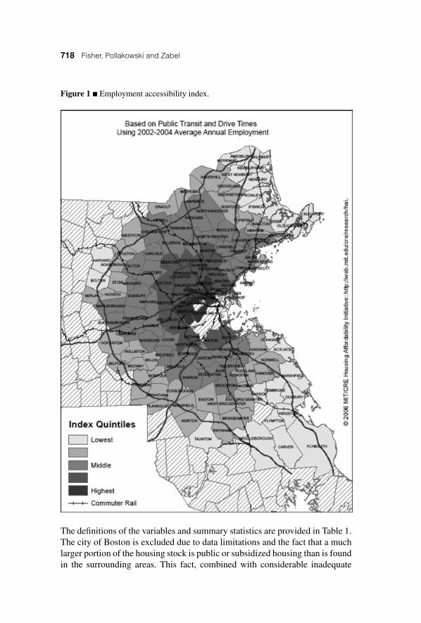
Town-level data on employment and commute times are used to construct thejob accessibility index (Figure 1). The index for town i is defined as
ACCESSi =∑j �=i
employmentj(commuteij)1.5
. (11)
This is a standard gravity index that measures access to employment as afunction of commuting time to each job. The town-level employment data,commuting data and methodology are described in Appendix 2. The indexvalue for any given town is the sum of employment in each destination townin the region divided by commuting time to that town. In Figure 1 we see thatthe Boston area remains strongly monocentric. About half of all employmentis located in the central area. Suburban subcenters account for much of theremaining employment.
The regression that we use includes the following structural characteristics:age, the number of bathrooms and bedrooms,9 lot size and its square, interiorsize and its square and whether the house is a cape, colonial or ranch style forsingle-family houses and whether it is a town-house for condominiums. Wealso include population density and the percent of open space in the town. Thethree town-level variables that we use to adjust town-level affordability are theaccessibility index, the sum of the 10th-grade English and math MassachusettsComprehensive Assessment System (MCAS) scores and a composite safetymeasure.10 Data on school scores are obtained from the Massachusetts Depart-ment of Education. Data on the variables employed to construct the compositesafety variable are obtained from several sources described in Appendix 2.
for advantages and disadvantages with regard to town-level amenities. Lerman andReeder’s goal is to indicate which poor households should receive subsidies. Our goalis to make transparent the affordable stock in a spatial setting, setting the stage for avariety of focused policies.9 One problem with the sales data is that the number of bedrooms is often unreported—in some cases for all observations in a town. In order to keep these observations in thedata set, we impute values for the number of bedrooms. We do this by regressing thenumber of bedrooms on the other structural characteristics for observations with at leastone bedroom. We then replace the observations with a missing value with the predictedvalue from the bedrooms regression.10 The MCAS scores are actually recorded as the percentage of students who score inthe proficient or advanced categories.
718 Fisher, Pollakowski and Zabel
Figure 1 � Employment accessibility index.
The definitions of the variables and summary statistics are provided in Table 1.The city of Boston is excluded due to data limitations and the fact that a muchlarger portion of the housing stock is public or subsidized housing than is foundin the surrounding areas. This fact, combined with considerable inadequate
Amenity-Based Housing Affordability Indexes 719
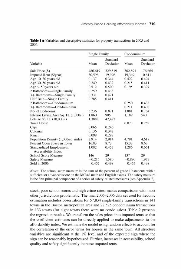
Table 1 � Variables and descriptive statistics for property transactions in 2005 and2006.
Single Family Condominium
Standard StandardVariable Mean Deviation Mean Deviation
Sale Price ($) 486,619 329,519 302,891 176,665Imputed Rent ($/year) 30,596 19,996 19,349 10,611Age 10–30 years old 0.137 0.344 0.422 0.494Age 30–50 years old 0.249 0.432 0.215 0.411Age > 50 years old 0.512 0.500 0.195 0.3972 Bathrooms—Single Family 0.259 0.4383+ Bathrooms—Single Family 0.331 0.471Half Bath—Single Family 0.785 0.4112 Bathrooms—Condominium 0.250 0.4333+ Bathrooms—Condominium 0.211 0.408No. of Bedrooms 3.236 0.871 1.881 0.784Interior Living Area Sq. Ft. (1,000s.) 1.860 905 1,189 540Lotsize Sq. Ft. (10,000s.) 1.3888 42,422Town House 0.073 0.259Cape 0.065 0.246Colonial 0.136 0.342Ranch 0.098 0.297Population Density (1,000/sq. mile) 2,914 2,914 4,791 4,618Percent Open Space in Town 16.83 8.73 15.33 8.63Standardized Employment 1.082 0.453 1.286 0.661
Accessibility IndexSchool Score Measure 146 29 137 29Safety Measure −0.215 1.580 −0.890 1.979Sold in 2006 0.457 0.498 0.455 0.498
Notes: The school score measure is the sum of the percent of grade 10 students with asufficient or advanced score on the MCAS math and English exams. The safety measureis the first principal component of a series of safety-related measures (see Appendix 2).
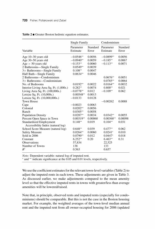
stock, poor school scores and high crime rates, makes comparisons with mostother jurisdictions problematic. The final 2005–2006 data set used for hedonicestimation includes observations for 57,834 single-family transactions in 141towns in the Boston metropolitan area and 22,525 condominium transactionsin 133 towns (for eight towns there were no condo sales). Table 2 presentsthe regression results. We transform the sales prices into imputed rents so thatthe coefficient estimates can be directly applied to make adjustments to theaffordability index. We estimate the model using random effects to account forthe correlation of the error terms for houses in the same town. All structurevariables are significant at the 1% level and of the expected sign where thesign can be reasonably hypothesized. Further, increases in accessibility, schoolquality and safety significantly increase imputed rents.
720 Fisher, Pollakowski and Zabel
Table 2 � Greater Boston hedonic equation estimates.
Single Family Condominium
Parameter Standard Parameter StandardVariable Estimate Error Estimate Error
Age 10–30 years old −0.0546∗∗ 0.0056 −0.0899∗∗ 0.0056Age 30–50 years old −0.0940∗∗ 0.0059 −0.185∗∗ 0.0067Age > 50 years old −0.153∗∗ 0.0060 −0.113∗∗ 0.00712 Bathrooms—Single Family 0.0549∗∗ 0.00393+ Bathrooms—Single Family 0.108∗∗ 0.0047Half Bath—Single Family 0.0634∗∗ 0.00462 Bathrooms—Condominium 0.0676∗∗ 0.00513+ Bathrooms—Condominium 0.0785∗∗ 0.0064No. of Bedrooms 0.0192∗∗ 0.0022 0.0164∗∗ 0.0032Interior Living Area Sq. Ft. (1,000s.) 0.282∗∗ 0.0074 0.800∗∗ 0.021Living Area Sq. Ft. (100,000s.) −0.0778∗∗ 0.012 −0.109∗∗ 0.062Lotsize Sq. Ft. (10,000s.) 0.00548∗∗ 0.0013Lotsize Sq. Ft. (10,000,000s.) −0.0133 0.0128Town House −0.00262 0.0088Cape −0.0023 0.0063Colonial 0.0202∗∗ 0.0056Ranch 0.0305∗∗ 0.0058Population Density 0.0287∗∗ 0.0034 0.0342∗∗ 0.0055Percent Open Space in Town 0.00319∗∗ 0.00060 0.00368∗∗ 0.00098Standardized Employment 0.148∗∗ 0.019 0.104∗∗ 0.031
Accessibility Index (natural log)School Score Measure (natural log) 0.648∗∗ 0.039 0.477∗∗ 0.062Safety Measure 0.0264∗∗ 0.0060 0.0241∗ 0.010Sold in 2006 0.0790∗∗ 0.012 0.0447∗ 0.018Constant 6.252∗∗ 0.20 6.463∗∗ 0.31Observations 57,834 22,525Number of Towns 138 133R2 0.563 0.657
Note: Dependent variable: natural log of imputed rent.∗ and ∗∗ indicate significance at the 0.05 and 0.01 levels, respectively.
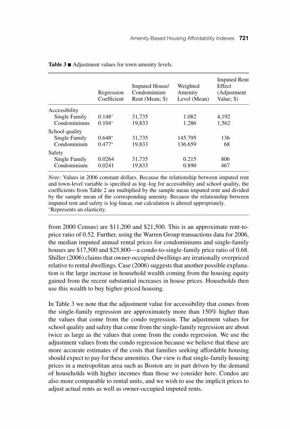
We use the coefficient estimates for the relevant town-level variables (Table 2) toadjust the imputed rents in each town. These adjustments are given in Table 3.As discussed earlier, we make adjustments compared to the mean amenitylevel so that the effective imputed rents in towns with greater/less than averageamenities will be lowered/raised.
Note that, in principle, observed rents and imputed rents (especially for condo-miniums) should be comparable. But this is not the case in the Boston housingmarket. For example, the weighted averages of the town-level median annualrent and the imputed rent from all owner-occupied housing for 2006 (updated
Amenity-Based Housing Affordability Indexes 721
Table 3 � Adjustment values for town amenity levels.
Imputed RentImputed House/ Weighted Effect
Regression Condominium Amenity (AdjustmentCoefficient Rent (Mean; $) Level (Mean) Value; $)
AccessibilitySingle Family 0.148∗ 31,735 1.082 4,192Condominiums 0.104∗ 19,833 1.286 1,562
School qualitySingle Family 0.648∗ 31,735 145.795 136Condominium 0.477∗ 19,833 136.659 68
SafetySingle Family 0.0264 31,735 0.215 806Condominium 0.0241 19,833 0.890 467
Note: Values in 2006 constant dollars. Because the relationship between imputed rentand town-level variable is specified as log–log for accessibility and school quality, thecoefficients from Table 2 are multiplied by the sample mean imputed rent and dividedby the sample mean of the corresponding amenity. Because the relationship betweenimputed rent and safety is log-linear, our calculation is altered appropriately.∗Represents an elasticity.
from 2000 Census) are $11,200 and $21,500. This is an approximate rent-to-price ratio of 0.52. Further, using the Warren Group transactions data for 2006,the median imputed annual rental prices for condominiums and single-familyhouses are $17,500 and $25,800—a condo-to-single-family price ratio of 0.68.Shiller (2006) claims that owner-occupied dwellings are irrationally overpricedrelative to rental dwellings. Case (2006) suggests that another possible explana-tion is the large increase in household wealth coming from the housing equitygained from the recent substantial increases in house prices. Households thenuse this wealth to buy higher-priced housing.
In Table 3 we note that the adjustment value for accessibility that comes fromthe single-family regression are approximately more than 150% higher thanthe values that come from the condo regression. The adjustment values forschool quality and safety that come from the single-family regression are abouttwice as large as the values that come from the condo regression. We use theadjustment values from the condo regression because we believe that these aremore accurate estimates of the costs that families seeking affordable housingshould expect to pay for these amenities. Our view is that single-family housingprices in a metropolitan area such as Boston are in part driven by the demandof households with higher incomes than those we consider here. Condos arealso more comparable to rental units, and we wish to use the implicit prices toadjust actual rents as well as owner-occupied imputed rents.
722 Fisher, Pollakowski and Zabel
Results
In this section, we present the results for the area affordability index for theBoston metropolitan area. We also compare the town rankings obtained fromour index with a simple ranking produced by a median house price index. Togenerate our index, we determine how many existing housing units are afford-able. We use the rule that units with rent (or rental-equivalent) that is no morethan 30% of household income are affordable (to that household). We calculatetwo indexes: two-person and four-person (two adults, two children) house-holds earning 80% of AMI. We then generate an overall affordability indexby taking a weighted average of these two indexes based on the fact that 75%of the population in the Boston area is one-to-three-person households (two-person) and 25% is households with four or more members (four-person).11
Note that this is our benchmark index; one of the advantages of our indexis that it can be constructed for any relevant household structure/size/incomecombination.
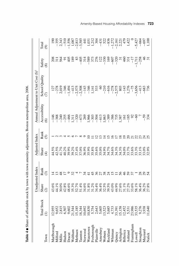
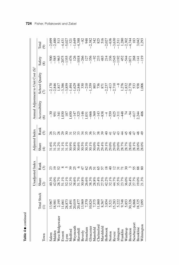
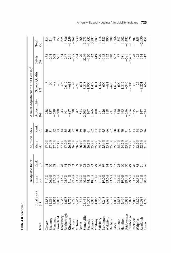
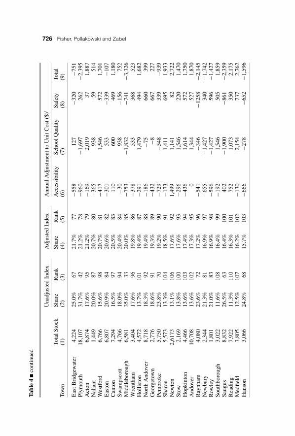
We begin by presenting the results that lead to our unadjusted affordable stock.Column (1) of Table 4 presents the total stock of dwellings—owner and rental—by town. Column (2) of Table 4 presents the percentage of each town’s stockthat is structurally adequate and affordable—this is our unadjusted index. Thisindex is presented in Figure 2, with the ordinal ranking of towns presented incolumn (3) of Table 4. Note that this unadjusted stock measure is not simply acount of all dwellings that appear affordable. To be included, dwellings mustbe structurally adequate, they must not be subsidized dwellings that are onlyappropriate for households of lower income than considered here and theymust have an appropriate number of bedrooms for the type of household beingconsidered (see Appendix 2).
To help motivate the importance of making amenity adjustments, in Table 5towns are grouped by quintile of the unadjusted affordable stock rankings. Atthe bottom of Table 5, we present the mean amenity scores for each quintile.Striking patterns emerge with respect to both school quality and safety. Thequintile containing the most affordable towns prior to amenity adjustmentsis marked by quite low school scores and safety ratings. This is particularlythe case for the 12 most affordable towns (not shown). As we move acrossthe table to less affordable town quintiles, the scores for school quality andsafety monotonically increase in a substantial manner. Mean job accessibilityis similar across quintiles. The reality underscoring this (lack of) relationshipcan be seen by comparing the relatively monocentric job accessibility index
11 Separate results for two-person and four-person households are available from theauthors.
Amenity-Based Housing Affordability Indexes 723Ta
ble
4�
Shar
eof
affo
rdab
lest
ock
byto
wn
with
tow
nam
enity
adju
stm
ents
,Bos
ton
met
ropo
litan
area
,200
6.
Una
djus
ted
Inde
xA
djus
ted
Inde
xA
nnua
lAdj
ustm
entt
oU
nitC
ost(
$)1
Tota
lSto
ckSh
are
Ran
kSh
are
Ran
kA
cces
sibi
lity
Scho
olQ
ualit
ySa
fety
Tota
lTo
wn
(1)
(2)
(3)
(4)
(5)
(6)
(7)
(8)
(9)
Mar
lbor
ough
12,9
5543
.6%
1444
.5%
1−1
4612
720
819
0M
ilfor
d9,
652
44.1
%13
42.5
%2
−388
−278
311
−355
Mill
is2,
815
30.0
%48
41.7
%3
−240
2,01
956
42,
343
Hud
son
6,50
742
.8%
1740
.2%
4−2
55−3
4691
−510
Dra
cut
9,60
248
.6%
939
.9%
5−4
66−1
,494
405
−1,5
56W
alth
am21
,544
35.3
%32
39.2
%6
1,31
1−4
1318
91,
087
Met
huen
15,1
8552
.7%
437
.4%
7−3
20−2
,575
83−2
,813
Taun
ton
18,3
4451
.4%
737
.0%
8−6
73−2
,508
−405
−3,5
85N
orw
ood
10,6
9234
.6%
3436
.9%
926
9−1
4331
444
1W
ater
tow
n10
,830
31.8
%41
35.9
%10
1,96
6−3
46−5
891,
031
Foxb
orou
gh5,
754
31.2
%45
35.8
%11
−303
1,14
137
31,
212
Plai
nvill
e2,
643
34.4
%36
35.6
%12
−504
533
276
304
Am
esbu
ry5,
605
36.4
%27
35.0
%13
−613
6012
2−4
31W
obur
n13
,523
32.5
%38
34.9
%14
1,06
3−2
10−3
3052
2R
ockl
and
5,68
539
.5%
2434
.7%
15−3
89−6
1616
9−8
36W
hitm
an4,
733
43.0
%15
34.6
%16
−386
−278
−607
−1,2
72Q
uinc
y33
,391
44.9
%11
34.3
%17
735
−2,5
75−3
20−2
,161
Arl
ingt
on15
,158
27.6
%56
34.3
%18
1,38
780
331
2,22
1B
iller
ica
12,4
5231
.1%
4634
.0%
1916
1−1
4346
047
9A
shla
nd5,
531
27.2
%59
33.7
%20
−185
1,27
633
11,
422
Fram
ingh
am23
,986
33.6
%37
33.6
%21
92− 7
5−1
70
Low
ell
33,5
3558
.1%
133
.3%
22−6
0−3
,656
−1,7
11−5
,427
Stou
ghto
n9,
276
36.4
%28
33.1
%23
7−4
13−2
58−6
64M
ayna
rd3,
938
36.2
%29
33.0
%24
−59
−683
46−6
97N
atic
k11
,640
27.8
%54
32.9
%25
334
736
311,
100
724 Fisher, Pollakowski and ZabelTa
ble
4�
cont
inue
d
Una
djus
ted
Inde
xA
djus
ted
Inde
xA
nnua
lAdj
ustm
entt
oU
nitC
ost(
$)1
Tota
lSto
ckSh
are
Ran
kSh
are
Ran
kA
cces
sibi
lity
Scho
olQ
ualit
ySa
fety
Tota
lTo
wn
(1)
(2)
(3)
(4)
(5)
(6)
(7)
(8)
(9)
Sale
m13
,967
40.3
%23
31.6
%26
−30
−2,1
70−5
00−2
,699
Mal
den
18,9
8142
.0%
1931
.2%
2795
1−2
,846
−585
−2,4
80W
estB
ridg
ewat
er2,
195
28.7
%52
31.2
%28
−341
1,81
7−9
6351
3E
vere
tt11
,661
51.1
%8
31.1
%29
1,03
0−3
,386
−207
5−4
,431
Lynn
28,8
7352
.1%
531
.1%
3018
7−3
,859
−135
5−5
,027
Med
ford
16,4
9132
.3%
3930
.9%
311,
650
−1,4
94−4
76−3
21W
eym
outh
20,0
1938
.6%
2530
.8%
32−1
47−1
,629
126
−1,6
49H
aver
hill
20,4
7751
.7%
630
.6%
33−5
25−2
,846
−101
8−4
,388
Bev
erly
13,9
6930
.8%
4730
.5%
34−1
4633
0−2
66−8
2St
oneh
am7,
570
26.6
%62
30.3
%35
1,03
1−2
1012
794
8G
louc
este
r10
,824
38.3
%26
30.1
%36
−666
−1,3
59−3
56−2
,382
Man
sfiel
d7,
575
28.8
%51
30.0
%37
−369
803
−92
342
Che
lmsf
ord
11,8
6025
.4%
6529
.4%
38−1
4373
623
382
5M
arsh
field
8,56
727
.5%
5729
.4%
39−8
3887
148
351
6H
olbr
ook
3,85
442
.2%
1829
.1%
40−4
−2,2
3721
4−2
,027
Nor
ton
5,52
132
.1%
4029
.0%
41−5
59−4
1333
6−6
36R
ever
e15
,283
44.7
%12
29.0
%42
625
−2,7
10−1
545
−3,6
30A
bing
ton
5,22
235
.5%
3129
.0%
43−3
11−8
−119
2−1
,511
Fran
klin
9,74
823
.7%
7128
.7%
44−4
481,
276
452
1,28
0W
inth
rop
5,85
336
.0%
3028
.7%
4574
−1,8
32−5
44−2
,302
Bro
ckto
n30
,326
54.4
%3
28.6
%46
−94
−2,7
78−1
871
−4,7
44N
ewbu
rypo
rt6,
866
27.7
%55
28.1
%47
−617
533
268
183
Bro
oklin
e18
,325
19.0
%88
28.0
%48
2,24
493
8−1
413,
042
Wilm
ingt
on7,
095
21.3
%80
28.0
%49
406
1,00
6−1
191,
293
Amenity-Based Housing Affordability Indexes 725Ta
ble
4�
cont
inue
d
Una
djus
ted
Inde
xA
djus
ted
Inde
xA
nnua
lAdj
ustm
entt
oU
nitC
ost(
$)1
Tota
lSto
ckSh
are
Ran
kSh
are
Ran
kA
cces
sibi
lity
Scho
olQ
ualit
ySa
fety
Tota
lTo
wn
(1)
(2)
(3)
(4)
(5)
(6)
(7)
(8)
(9)
Car
ver
2,85
131
.3%
4427
.9%
50−9
58−8
432
−534
Bra
intr
ee11
,836
26.9
%60
27.9
%51
357
60−2
0421
4M
erri
mac
1,96
227
.5%
5827
.5%
52−6
39−8
638
−9G
rove
land
2,08
326
.8%
6127
.4%
53−5
00−8
661
153
Tew
ksbu
ry9,
386
23.5
%78
27.4
%54
4339
818
462
5B
oxbo
roug
h1,
693
25.5
%64
27.2
%55
−401
2,01
926
71,
886
Kin
gsto
n3,
756
31.4
%43
26.7
%56
−817
−683
241
−1,2
59D
anve
rs8,
795
27.9
%53
26.5
%57
70−1
43−2
95−3
68M
elro
se9,
451
23.9
%69
26.5
%58
847
−210
294
930
Ber
lin82
225
.2%
6626
.4%
59−5
3387
1−7
026
8So
mer
ville
24,4
3140
.6%
2226
.4%
602,
295
−3,3
18−2
249
−3,2
73Pe
abod
y16
,557
34.4
%35
26.2
%61
167
−1,9
00−1
20−1
,852
Bel
mon
t7,
973
18.2
%93
25.7
%62
1,76
61,
479
423,
287
Med
way
4,06
322
.0%
7925
.7%
63−4
0087
141
988
9Sa
lisbu
ry2,
723
41.7
%20
25.5
%64
−721
−1,4
27−1
570
−3,7
18B
urlin
gton
8,24
819
.0%
8925
.4%
6592
660
0−1
431,
383
Wak
efiel
d8,
687
23.6
%74
25.1
%66
718
−481
152
390
Ded
ham
8,17
723
.6%
7325
.0%
6773
1−6
8324
028
8E
ssex
1,09
721
.1%
8225
.0%
68−6
341,
614
687
1,66
6L
ittle
ton
2,83
523
.6%
7525
.0%
69−3
2060
067
347
Ham
ilton
2,46
619
.0%
9024
.2%
70−4
951,
817
581
1,90
2B
ridg
ewat
er6,
921
29.4
%50
23.7
%71
−556
−346
−581
−1,4
82C
ambr
idge
33,0
2129
.6%
4923
.2%
722,
914
−2,3
05−2
,437
−1,8
28R
ockp
ort
3,09
023
.5%
7622
.9%
73−8
1533
017
8−
307
Wal
pole
7,82
920
.5%
8522
.7%
74−7
112
749
855
5R
ando
lph
10,3
8741
.1%
2122
.5%
7514
7−3
,251
174
−2,9
30Ip
swic
h4,
780
20.4
%86
21.8
%76
−634
668
417
451
726 Fisher, Pollakowski and ZabelTa
ble
4�
cont
inue
d
Una
djus
ted
Inde
xA
djus
ted
Inde
xA
nnua
lAdj
ustm
entt
oU
nitC
ost(
$)1
Tota
lSto
ckSh
are
Ran
kSh
are
Ran
kA
cces
sibi
lity
Scho
olQ
ualit
ySa
fety
Tota
lTo
wn
(1)
(2)
(3)
(4)
(5)
(6)
(7)
(8)
(9)
Eas
tBri
dgew
ater
4,22
425
.0%
6721
.7%
77−5
5812
7−3
20−7
51Pl
ymou
th18
,107
31.7
%42
21.2
%78
−960
−1,6
9726
2−2
,395
Act
on6,
874
17.6
%95
21.2
%79
−169
2,01
937
1,88
7N
ahan
t1,
449
20.0
%87
20.7
%80
−365
938
−59
514
Wes
tfor
d6,
766
15.6
%98
20.7
%81
−417
1,54
657
21,
701
Eas
ton
6,80
720
.9%
8420
.6%
82−3
0153
3−3
39−1
07C
anto
n7,
294
16.5
%97
20.5
%83
110
600
469
1,18
0Sw
amps
cott
4,76
618
.0%
9420
.4%
84−3
093
8−1
5675
2M
iddl
ebor
ough
6,58
135
.0%
3320
.0%
85−7
53−1
,832
−741
−3,3
26W
rent
ham
3,40
417
.6%
9619
.8%
86−3
7853
336
852
3H
ollis
ton
4,57
213
.7%
101
19.4
%87
−291
1,47
949
41,
682
Nor
thA
ndov
er8,
718
18.3
%92
19.4
%88
−186
−75
660
399
Geo
rget
own
2,77
618
.6%
9119
.3%
89−4
32−8
667
227
Pem
brok
e5,
750
23.8
%70
19.2
%90
−729
−548
339
−939
Shar
on5,
573
13.3
%10
418
.5%
91−1
731,
411
695
1,93
3N
ewto
n2,
6173
13.1
%10
617
.6%
921,
499
1,14
182
2,72
2St
ow2,
169
13.8
%10
017
.6%
93−2
961,
546
220
1,47
0H
opki
nton
4,46
613
.6%
103
17.4
%94
−436
1,61
457
21,
750
And
over
10,7
0813
.6%
102
17.3
%95
01,
344
527
1,87
0R
aynh
am4,
080
23.6
%72
17.2
%96
−541
−346
−125
8−2
,145
New
bury
2,34
421
.3%
8116
.9%
97−6
55−1
,427
340
−1,7
42R
owle
y1,
801
21.0
%83
16.9
%98
−596
−1,4
2759
6−1
,427
Sout
hbor
ough
3,02
211
.6%
108
16.4
%99
−192
1,54
650
51,
859
Saug
us8,
832
26.5
%63
16.4
%10
040
2−1
,900
−861
−2,3
59R
eadi
ng7,
922
11.3
%11
016
.3%
101
752
1,07
335
02,
175
Med
field
3,80
512
.5%
107
16.2
%10
2−1
302,
154
737
2,76
2H
anso
n3,
066
24.8
%68
15.7
%10
3−6
66−2
78−6
52−1
,596

Amenity-Based Housing Affordability Indexes 727Ta
ble
4�
cont
inue
d
Una
djus
ted
Inde
xA
djus
ted
Inde
xA
nnua
lAdj
ustm
entt
oU
nitC
ost(
$)1
Tota
lSto
ckSh
are
Ran
kSh
are
Ran
kA
cces
sibi
lity
Scho
olQ
ualit
ySa
fety
Tota
lTo
wn
(1)
(2)
(3)
(4)
(5)
(6)
(7)
(8)
(9)
Man
ches
ter
1,98
514
.4%
9915
.5%
104
−497
1,61
4−8
1,10
9N
orth
Rea
ding
4,49
111
.0%
111
15.1
%10
517
566
848
81,
331
Hul
l4,
023
23.5
%77
14.9
%10
6−7
50−2
,373
238
−2,8
85A
von
1,59
842
.9%
1613
.9%
107
94−3
,994
−118
8−5
,088
Scitu
ate
6,49
810
.6%
113
13.0
%10
8−7
861,
276
567
1,05
7H
anov
er4,
398
11.4
%10
912
.7%
109
−485
600
417
533
Hin
gham
6,78
89.
2%11
512
.6%
110
−448
1,74
954
11,
843
Win
ches
ter
7,03
78.
1%11
912
.1%
111
1248
1,68
224
13,
170
Nor
folk
2,82
910
.3%
114
11.9
%11
2−3
9133
075
169
0H
arva
rd1,
601
8.2%
118
11.6
%11
3−6
422,
087
306
1,75
1W
estw
ood
4,69
56.
8%12
211
.3%
114
483
1,74
956
32,
795
Mar
bleh
ead
7,73
310
.9%
112
11.2
%11
5−3
6687
1−2
7522
9N
eedh
am9,
959
6.0%
126
10.9
%11
686
31,
884
520
3,26
7B
edfo
rd4,
385
8.2%
117
10.9
%11
750
566
865
91,
831
Law
renc
e2,
0769
57.0
%2
10.3
%11
8−1
02−7
,237
−215
7−9
,497
Milt
on8,
023
8.3%
116
10.3
%11
973
4−2
1033
185
5L
inco
ln1,
788
7.2%
120
9.4%
120
653
1,68
267
63,
011
Coh
asse
t2,
460
6.9%
121
8.3%
121
−750
2,08
743
91,
777
Lex
ingt
on10
,577
4.1%
134
8.3%
122
967
1,61
463
43,
215
Mid
dlet
on2,
373
13.1
%10
58.
0%12
3−1
20−2
,710
538
−2,2
92C
onco
rd5,
462
5.9%
127
8.0%
124
133
1,88
451
22,
529
Tops
field
1,91
86.
5%12
37.
7%12
5−2
9593
852
21,
166
Dux
bury
4,54
36.
4%12
47.
7%12
6−7
9193
867
882
5B
olto
n1,
363
5.2%
129
7.2%
127
−614
1,54
611
21,
045
Wes
ton
3,62
05.
4%12
87.
0%12
875
42,
290
751
3,79
5W
elle
sley
8,18
64.
9%13
06.
9%12
977
61,
682
411
2,86
9
728 Fisher, Pollakowski and Zabel
Tabl
e4
�co
ntin
ued
Una
djus
ted
Inde
xA
djus
ted
Inde
xA
nnua
lAdj
ustm
entt
oU
nitC
ost(
$)1
Tota
lSto
ckSh
are
Ran
kSh
are
Ran
kA
cces
sibi
lity
Scho
olQ
ualit
ySa
fety
Tota
lTo
wn
(1)
(2)
(3)
(4)
(5)
(6)
(7)
(8)
(9)
Che
lsea
9,52
448
.4%
106.
8%13
084
4−5
,751
−324
9−8
,156
Nor
wel
l3,
200
4.6%
132
6.6%
131
−527
1,68
221
71,
371
Wen
ham
1,16
54.
2%13
36.
1%13
2−3
411,
817
632
2,10
8W
ayla
nd4,
470
3.2%
137
6.0%
133
275
2,35
753
93,
172
Sudb
ury
5,52
33.
6%13
55.
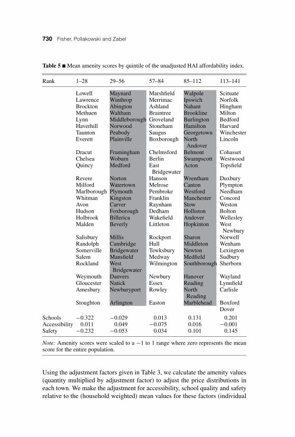
1%13
4−9
61,
682
640
2,22
6Sh
erbo
rn1,
288
3.5%
136
5.0%
135
−142
2,56
056
62,
984
Lynn
field
3,80
43.
1%13
84.
7%13
633
31,
479
−41
1,77
0W
estN
ewbu
ry1,
299
4.7%
131
4.6%
137
−591
−854
7−5
2Pl
ympt
on73
36.
4%12
54.
0%13
8−8
60−6
83−3
14−1
,857
Dov
er1,
705
1.7%
141
2.9%
139
292,
560
746
3,33
5C
arlis
le1,
440
1.8%
139
2.4%
140
−116
1,88
426
62,
035
Box
ford
2,35
91.
7%14
02.
4%14
1−4
4793
866
71,
158
Not
e:N
=14
1.A
llho
useh
olds
at80
%B
osto
nm
etro
polit
anar
eam
edia
nin
com
e.
Amenity-Based Housing Affordability Indexes 729
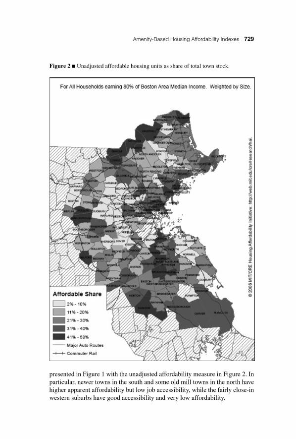
Figure 2 � Unadjusted affordable housing units as share of total town stock.
presented in Figure 1 with the unadjusted affordability measure in Figure 2. Inparticular, newer towns in the south and some old mill towns in the north havehigher apparent affordability but low job accessibility, while the fairly close-inwestern suburbs have good accessibility and very low affordability.
730 Fisher, Pollakowski and Zabel
Table 5 � Mean amenity scores by quintile of the unadjusted HAI affordability index.
Rank 1–28 29–56 57–84 85–112 113–141
Lowell Maynard Marshfield Walpole ScituateLawrence Winthrop Merrimac Ipswich NorfolkBrockton Abington Ashland Nahant HinghamMethuen Waltham Braintree Brookline MiltonLynn Middleborough Groveland Burlington BedfordHaverhill Norwood Stoneham Hamilton HarvardTaunton Peabody Saugus Georgetown WinchesterEverett Plainville Boxborough North Lincoln
AndoverDracut Framingham Chelmsford Belmont CohassetChelsea Woburn Berlin Swampscott WestwoodQuincy Medford East Acton Topsfield
BridgewaterRevere Norton Hanson Wrentham DuxburyMilford Watertown Melrose Canton PlymptonMarlborough Plymouth Pembroke Westford NeedhamWhitman Kingston Franklin Manchester ConcordAvon Carver Raynham Stow WestonHudson Foxborough Dedham Holliston BoltonHolbrook Billerica Wakefield Andover WellesleyMalden Beverly Littleton Hopkinton West
NewburySalisbury Millis Rockport Sharon NorwellRandolph Cambridge Hull Middleton WenhamSomerville Bridgewater Tewksbury Newton LexingtonSalem Mansfield Medway Medfield SudburyRockland West Wilmington Southborough Sherborn
BridgewaterWeymouth Danvers Newbury Hanover WaylandGloucester Natick Essex Reading LynnfieldAmesbury Newburyport Rowley North Carlisle
ReadingStoughton Arlington Easton Marblehead Boxford
Dover
Schools −0.322 −0.029 0.013 0.131 0.201Accessibility 0.011 0.049 −0.075 0.016 −0.001Safety −0.232 −0.053 0.034 0.101 0.145
Note: Amenity scores were scaled to a −1 to 1 range where zero represents the meanscore for the entire population.
Using the adjustment factors given in Table 3, we calculate the amenity values(quantity multiplied by adjustment factor) to adjust the price distributions ineach town. We make the adjustment for accessibility, school quality and safetyrelative to the (household weighted) mean values for these factors (individual
Amenity-Based Housing Affordability Indexes 731
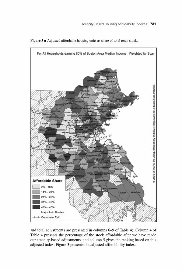
Figure 3 � Adjusted affordable housing units as share of total town stock.
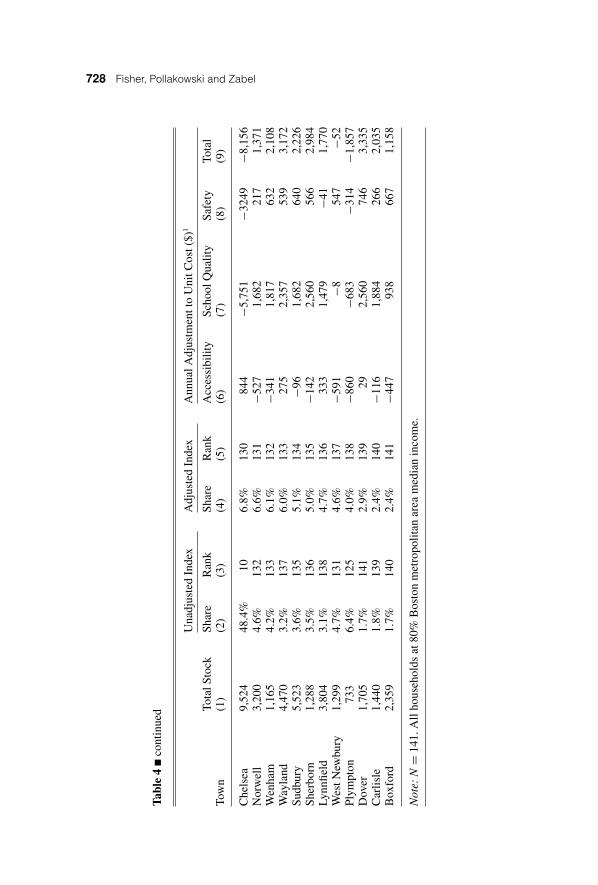
and total adjustments are presented in columns 6–9 of Table 4). Column 4 ofTable 4 presents the percentage of the stock affordable after we have madeour amenity-based adjustments, and column 5 gives the ranking based on thisadjusted index. Figure 3 presents the adjusted affordability index.
732 Fisher, Pollakowski and Zabel
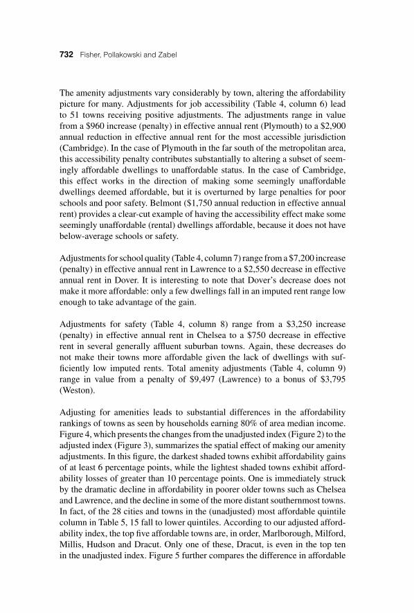
The amenity adjustments vary considerably by town, altering the affordabilitypicture for many. Adjustments for job accessibility (Table 4, column 6) leadto 51 towns receiving positive adjustments. The adjustments range in valuefrom a $960 increase (penalty) in effective annual rent (Plymouth) to a $2,900annual reduction in effective annual rent for the most accessible jurisdiction(Cambridge). In the case of Plymouth in the far south of the metropolitan area,this accessibility penalty contributes substantially to altering a subset of seem-ingly affordable dwellings to unaffordable status. In the case of Cambridge,this effect works in the direction of making some seemingly unaffordabledwellings deemed affordable, but it is overturned by large penalties for poorschools and poor safety. Belmont ($1,750 annual reduction in effective annualrent) provides a clear-cut example of having the accessibility effect make someseemingly unaffordable (rental) dwellings affordable, because it does not havebelow-average schools or safety.
Adjustments for school quality (Table 4, column 7) range from a $7,200 increase(penalty) in effective annual rent in Lawrence to a $2,550 decrease in effectiveannual rent in Dover. It is interesting to note that Dover’s decrease does notmake it more affordable: only a few dwellings fall in an imputed rent range lowenough to take advantage of the gain.
Adjustments for safety (Table 4, column 8) range from a $3,250 increase(penalty) in effective annual rent in Chelsea to a $750 decrease in effectiverent in several generally affluent suburban towns. Again, these decreases donot make their towns more affordable given the lack of dwellings with suf-ficiently low imputed rents. Total amenity adjustments (Table 4, column 9)range in value from a penalty of $9,497 (Lawrence) to a bonus of $3,795(Weston).
Adjusting for amenities leads to substantial differences in the affordabilityrankings of towns as seen by households earning 80% of area median income.Figure 4, which presents the changes from the unadjusted index (Figure 2) to theadjusted index (Figure 3), summarizes the spatial effect of making our amenityadjustments. In this figure, the darkest shaded towns exhibit affordability gainsof at least 6 percentage points, while the lightest shaded towns exhibit afford-ability losses of greater than 10 percentage points. One is immediately struckby the dramatic decline in affordability in poorer older towns such as Chelseaand Lawrence, and the decline in some of the more distant southernmost towns.In fact, of the 28 cities and towns in the (unadjusted) most affordable quintilecolumn in Table 5, 15 fall to lower quintiles. According to our adjusted afford-ability index, the top five affordable towns are, in order, Marlborough, Milford,Millis, Hudson and Dracut. Only one of these, Dracut, is even in the top tenin the unadjusted index. Figure 5 further compares the difference in affordable

Amenity-Based Housing Affordability Indexes 733
Figure 4 � Effect of amenity adjustments on town-level housing affordability.
share of housing by the unadjusted and adjusted measures. While 60% of thetowns are deemed more affordable once the adjustments are made, the greatestvariance is for towns with upward adjustments to housing costs, and hencedecreases in affordable housing share.
734 Fisher, Pollakowski and Zabel
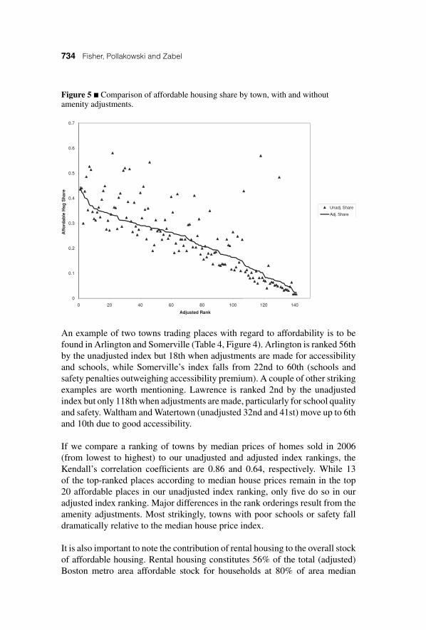
Figure 5 � Comparison of affordable housing share by town, with and withoutamenity adjustments.
0
0.1
0.2
0.3
0.4
0.5
0.6
0.7
0 20 40 60 80 100 120 140
Aff
ord
able
Hsg
Sh
are
Adjusted Rank
Unadj. Share
Adj. Share
An example of two towns trading places with regard to affordability is to befound in Arlington and Somerville (Table 4, Figure 4). Arlington is ranked 56thby the unadjusted index but 18th when adjustments are made for accessibilityand schools, while Somerville’s index falls from 22nd to 60th (schools andsafety penalties outweighing accessibility premium). A couple of other strikingexamples are worth mentioning. Lawrence is ranked 2nd by the unadjustedindex but only 118th when adjustments are made, particularly for school qualityand safety. Waltham and Watertown (unadjusted 32nd and 41st) move up to 6thand 10th due to good accessibility.
If we compare a ranking of towns by median prices of homes sold in 2006(from lowest to highest) to our unadjusted and adjusted index rankings, theKendall’s correlation coefficients are 0.86 and 0.64, respectively. While 13of the top-ranked places according to median house prices remain in the top20 affordable places in our unadjusted index ranking, only five do so in ouradjusted index ranking. Major differences in the rank orderings result from theamenity adjustments. Most strikingly, towns with poor schools or safety falldramatically relative to the median house price index.
It is also important to note the contribution of rental housing to the overall stockof affordable housing. Rental housing constitutes 56% of the total (adjusted)Boston metro area affordable stock for households at 80% of area median

Amenity-Based Housing Affordability Indexes 735
income. Table 6 presents the total share of adjusted affordable housing (relativeto the total housing stock) by tenure for the 35 most affordable towns. Thetowns that rank in the top 20 affordable shares for each tenure category areshown in bold. In these most affordable towns, there is variation in the shareof their affordable stocks by tenure. For example, Dracut’s affordable stockis dominated by owner-occupied housing, while Milford has a fairly equaldistribution. Waltham and Watertown’s affordable stocks are dominated byrental housing.
Even after making our adjustments, we observe a striking geographic dispersionof towns that are more or less affordable. The accessibility index developedhere has only a 20% simple correlation with the ex ante affordable share ofhousing by town. This is not a result to be expected unless severe location-specific constraints have been place on development and redevelopment. Wethus conjecture that much of the remaining variation in the location of affordablehousing in the region is related to the stringent land use regulation that existsin the Boston area. The swath of low affordability (less than 10% of the stockaffordable) in the fairly close-in affluent western suburbs in Figure 3 standsout in particular. These towns generally have better than average accessibility;however, such accessibility-based adjustments to the distribution of annualrents did not yield much change in the housing stock judged as affordable.This is because there are few dwellings in these locations with low enoughprices/rents to be affected by the adjustments.
Policy Implications
The index provides a rich framework for considering affordability in a supply-constrained housing market. It provides an improved methodology for assessingthe inventory of adequate housing that is affordable to different households ata certain level of location-related quality. It does not require that the dwellingunits be subsidized or otherwise linked to a public program, but it attemptsto assess the full distribution of privately owned housing that meets certainstandards of not only structural adequacy, but also of town quality that arecrucial in terms of opportunities faced by households. Thus the index allowstowns and policy makers to better understand the affordability of towns relativeto their peers in a more comprehensive manner. In addition, this methodologycalls for a broader discussion and refinement of the criteria by which societyjudges the suitability of affordable housing, especially with respect to schoolsand other local amenities.
Policy decisions made with average or aggregated measures of affordability areunlikely to succeed, at best, and risk squandering limited housing resources,at worst. Such policies fail to account for the opportunity costs and benefits of
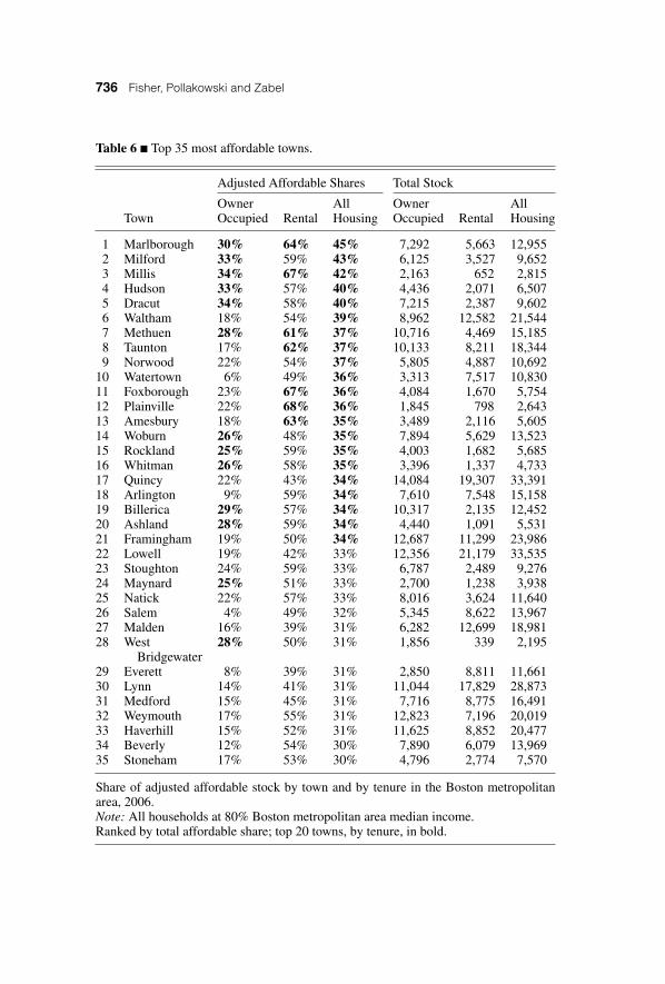
736 Fisher, Pollakowski and Zabel
Table 6 � Top 35 most affordable towns.
Adjusted Affordable Shares Total Stock
Owner All Owner AllTown Occupied Rental Housing Occupied Rental Housing
1 Marlborough 30% 64% 45% 7,292 5,663 12,9552 Milford 33% 59% 43% 6,125 3,527 9,6523 Millis 34% 67% 42% 2,163 652 2,8154 Hudson 33% 57% 40% 4,436 2,071 6,5075 Dracut 34% 58% 40% 7,215 2,387 9,6026 Waltham 18% 54% 39% 8,962 12,582 21,5447 Methuen 28% 61% 37% 10,716 4,469 15,1858 Taunton 17% 62% 37% 10,133 8,211 18,3449 Norwood 22% 54% 37% 5,805 4,887 10,692
10 Watertown 6% 49% 36% 3,313 7,517 10,83011 Foxborough 23% 67% 36% 4,084 1,670 5,75412 Plainville 22% 68% 36% 1,845 798 2,64313 Amesbury 18% 63% 35% 3,489 2,116 5,60514 Woburn 26% 48% 35% 7,894 5,629 13,52315 Rockland 25% 59% 35% 4,003 1,682 5,68516 Whitman 26% 58% 35% 3,396 1,337 4,73317 Quincy 22% 43% 34% 14,084 19,307 33,39118 Arlington 9% 59% 34% 7,610 7,548 15,15819 Billerica 29% 57% 34% 10,317 2,135 12,45220 Ashland 28% 59% 34% 4,440 1,091 5,53121 Framingham 19% 50% 34% 12,687 11,299 23,98622 Lowell 19% 42% 33% 12,356 21,179 33,53523 Stoughton 24% 59% 33% 6,787 2,489 9,27624 Maynard 25% 51% 33% 2,700 1,238 3,93825 Natick 22% 57% 33% 8,016 3,624 11,64026 Salem 4% 49% 32% 5,345 8,622 13,96727 Malden 16% 39% 31% 6,282 12,699 18,98128 West 28% 50% 31% 1,856 339 2,195
Bridgewater29 Everett 8% 39% 31% 2,850 8,811 11,66130 Lynn 14% 41% 31% 11,044 17,829 28,87331 Medford 15% 45% 31% 7,716 8,775 16,49132 Weymouth 17% 55% 31% 12,823 7,196 20,01933 Haverhill 15% 52% 31% 11,625 8,852 20,47734 Beverly 12% 54% 30% 7,890 6,079 13,96935 Stoneham 17% 53% 30% 4,796 2,774 7,570
Share of adjusted affordable stock by town and by tenure in the Boston metropolitanarea, 2006.Note: All households at 80% Boston metropolitan area median income.Ranked by total affordable share; top 20 towns, by tenure, in bold.
Amenity-Based Housing Affordability Indexes 737
local amenities associated with housing. For example, in the density overrideprogram in place in Massachusetts, developers must offer an affordable unit ofnewly developed housing at a rent of approximately $1,100 per month for a four-person household. This rent is set regardless of location. However, applyingour adjustments to monthly rent based on employment and school opportunityand safety, a unit in Wilmington would be worth approximately $475 morethan a unit in Everett (low school quality, high accessibility, low safety) butapproximately $160 less than the same unit in Belmont (high accessibility,above-average schools, above-average safety). If $1,100 was a firm cut-off forthe expenditure that a household should make on housing, then the affordableunit provided in Everett for a sticker price of $1,100 a month is, in fact, notaffordable to the targeted household. A household incurs an additional $400 incosts per month from living in Everett despite the amount they write on theirrent check each month. The cost incurred at that particular location is the neteffect of poor schools and poor safety loss, and the gains are from being locatednear many job opportunities.
Consider a town with limited affordable housing and struggling schools. Poli-cies based on a narrow affordability measure would likely direct housing invest-ments here. Frequently, such policy makers establish a single rent or “sticker”price for subsidized housing based on income level without accounting for theopportunity costs and benefits of residing in any given location. If a householdhas a fixed amount to spend, then accounting for job accessibility, school qualityand safety matters for the utility of the unit to the targeted households. Withoutsome prior (if not simultaneous) efforts to improve the overall quality of thearea for firms and households, desirable improvements in school performanceare doubtful and the subsidized rent for these units may still be too high. Asan extreme case, consider the town of Lawrence. The cost of having the lowestquality schools contributes to a drop in the rankings from 2nd (unadjusted)to 117th (adjusted). Economic development may be as important as additionalhousing investment in this place because, as it stands, there is an extraordinarilyhigh opportunity cost for households who locate in Lawrence. Therefore, theaffordability of the area might be improved not by building additional housingbut by improving the school system and other public amenities, as well as othereconomic development efforts. On the other hand, if housing investment is apriority in Lawrence, the subsidized price of the housing units should be ad-justed downward to account for the additional costs incurred by these housingmarket participants.
Some towns are categorized as unaffordable by the index because they arelocated far away from jobs. Such places with low job accessibility may notbe good candidates for affordable housing investment either. The literatureon spatial mismatch predicts inferior labor market outcomes for individual
738 Fisher, Pollakowski and Zabel
households who reside further from jobs due to higher search costs. Searchintensities are further worsened when households do not have access to a privatevehicle (Patacchini and Zenou 2005). From a regional perspective, spreadingout households far away from jobs may also raise the cost of labor therebyreducing the competitiveness of the region.
Our index also has the potential for controlling for factors other than job ac-cessibility, school quality and safety if it is felt that a particular demographicgroup responds to different locational characteristics. For example, senior cit-izens might not be as interested in living in towns with high accessibility andgood schools as they are in towns that have greater levels of safety. This shouldmake our index particularly useful because it can be applied to a broad rangeof affordable housing policies.
Conclusions
This article develops a new measure of affordable housing stock in a metropoli-tan area. When we consider town-specific amenities, we see major changes ineffective affordability. For households earning 80% of AMI, we find substantialshifts in affordability away from towns with poor job accessibility, poor schoolsand lack of safety.
These results are obtained from an effort to address housing affordability formoderate-income households in high-cost, supply-constrained coastal citiessuch as Boston. In Massachusetts, stringent town-level land use restrictions ren-der construction of (higher-density) housing for moderate-income householdsnearly infeasible. A first-best solution of region-wide relaxation of stringentlocal controls is not on the horizon. This article thus examines the renting andowning affordability implications for households earning between 50% and80% of area median income. To do this, we examine the distribution of hous-ing opportunities by location, quality and price/rents facing new entrants andother marginal households deciding whether to stay or leave. We develop a newmeasure of area affordability that characterizes the supply of housing that isaffordable to different households in different areas of the Boston metropolitanregion.
Key to our approach is the explicit recognition that the price/rent of a dwellingis affected by its location. Hence, we adjust our index to account for jobaccessibility, school quality and safety. This adjustment is based on obtainingimplicit prices of these amenities from a hedonic price equation. Housing atprices/rents that are unaffordable in the absence of location factors, for example,may be deemed affordable once strong job accessibility is considered. Ourmethodology makes transparent amenity-adjusted, town-level affordability of
Amenity-Based Housing Affordability Indexes 739
rental and owner stock, and it can support a menu of policy options to increaseaffordability.
The affordability index developed in this article suggests that not all places areequal. While policies that require towns to bear their fair share of a region’saffordable housing are politically popular, the implications for households, theregional economy and society generally are less favorable than a policy whichbetter accounts for the implications of location. While it should be no surpriseto anyone that location matters, this work strengthens our understanding oflocation in the linkages between housing, opportunity and regional economicsuccess.
By introducing our new concept of area affordability, we place emphasis onlocation because price/rent includes the value of the services provided by thelocal amenities. Further, the goal of affordable housing policy should be notonly to provide suitable structures for households but also to supply units thatare accessible to jobs, are in safe areas and have decent schools. Examining thisamenity-adjusted index in the Boston metropolitan area, it is clear that localamenities make a substantial difference in the relative affordability of towns.We demonstrate that town affordability for households earning 80% of AMIchanges substantially for a great many.
Our approach supports a menu of policy options in response to the particularaffordability problem uncovered in our index. For example, towns that arenot affordable because of inadequate schools may require alternate forms ofinvestment prior to new housing development. Such investment would aim toimprove the overall desirability of the area for firms and households, whichmay in turn improve school performance. Also, towns that are categorized asunaffordable by the index because they are located far from jobs may not begood candidates for affordable housing investment. Building new units far fromjobs may also raise the cost of labor, thereby reducing the competitiveness ofthe region in attracting and retaining firms. This ability to produce multipleoptions for dealing with the lack of affordable housing should make our indexparticularly useful to policy makers seeking a more flexible approach for dealingwith affordability issues in supply-constrained, high-cost areas such as Boston.
We appreciate the support of the MIT-CRE Housing Affordability Initiative.In particular, we thank Ryan McCann, Sheharyar Bokhari, Jessica Hau-rin, Andrew Jakabovics and Farooq Pasha for their help and excellent re-search assistance. Also, we are indebted to the Warren Group and the Cen-tral Transportation Planning Staff of Boston for their data contributions. Wethank Richard Arnott, Kyung-Hwan Kim, Tony Yezer and participants at the2006 AREUEA Mid-year Meetings in Washington, DC, the 2006 AREUEA

740 Fisher, Pollakowski and Zabel
International meetings in Vancouver and the 2006 Regional Science Associ-ation meetings in Toronto for helpful comments. Finally, we appreciate thecomments and suggestions of the editor and several referees.
References
Aslund, O., J. Osth and Y. Zenou. 2006. How Important is Access to Jobs? Old Question–Improved Answer. IZA Discussion Paper No. 2051.Bogdon, A.S. and A. Can. 1997. Indicators of Local Housing Affordability: Comparativeand Spatial Approaches. Real Estate Economics 25: 43–80.Brueckner, J.K. 1987. The Structure of Urban Equilibria: A Unified Treatment of theMuth–Mills Model. E.S. Mills, editor. Handbook of Regional and Urban Economics,Chapter 20. North-Holland: Amsterdam.Case, K.E. 2006. Land and Property Price Appreciation in Selected U.S. Cities: AHistorical Analysis. Paper prepared for Land Policies for Urban Development, LincolnInstitute for Land Policy, Cambridge, MA.Fujita, M. 1989. Urban Economic Theory. Cambridge University Press: Cambridge,UK.Glaeser, E. and J. Gyourko 2002. The Impact of Zoning on Housing Affordability.NBER Working Paper 8835.Goodman, J. and D. Rodda. 2005. Recent House Price Trends and Homeowner-ship Affordability. U.S. Department of Housing and Urban Development, Office ofPolicy Development and Research. Available at http://www.huduser.org/publications/affhsg/RecentHousePrice.html.Gyourko, J. and P.D. Linneman. 1993. The Affordability of the American Dream: AnExamination of the Last Thirty Years. Journal of Housing Research 1: 39–72.Gyourko, J., C. Mayer and T. Sinai. 2006. Superstar Cities. NBER Working paper12355.Gyourko, J. and J. Tracy. 1999. A Look at Real Housing Prices and Incomes: SomeImplications for Housing Affordability and Quality. Economic Policy Review, FederalReserve Bank of New York (September): 63–77.Lerman, D.L. and W.J. Reeder. 1987. The Affordability of Adequate Housing. AmericanReal Estate and Urban Economics Association Journal 15(4): 389–404.Patacchini, E. and Y. Zenou. 2005. Spatial Mismatch, Transport Mode, and SearchDecisions in England. Journal of Urban Economics 58: 62–90.Poterba, J. 1992. Taxation and Housing: Old Questions, New Answers. American Eco-nomic Review 82: 237–242.Quigley, J. and S. Raphael. 2005. Regulation and the High Cost of Housing in California.American Economic Review 95: 323–329.Saks, R. 2005. Job Creation and Housing Construction: Constraints on MetropolitanArea Employment Growth. Finance and Economics Discussion Series 2005-49. FederalReserve Board, Washington DC.Savage, Howard A. 2007. Who Could Afford to Buy a Home in 2002? Cur-rent Housing Reports, U.S. Bureau of the Census. Available at http://www.census.gov/prod/2007pubs/h121-07-1.pdfShiller, R. 2006. Long-Term Perspectives on the Current Boom in Home Prices.Economists’ Voice 3(4): 1–11.Sieg, H., V.K. Smith, H.S. Banzhaf and R.Walsh. 2002. Interjurisdictional HousingPrices in Locational Equilibrium. Journal of Urban Economics 52: 131–153.
Amenity-Based Housing Affordability Indexes 741
U.S. Department of Housing and Urban Development. 1998. Cranston-GonzalezNational Affordable Housing Act, Title II. Available at http://www.hud.gov/offices/cpd/affordablehousing/lawsandregs/laws/home/homelaws.pdf.U.S. Department of Housing & Urban Development, Office of Policy Development& Research. 2007. April (rev.). Fair Market Rents for the Section 8 Housing Assis-tance Payments Program. Retrieved from the HUD USER website: http://www.huduser.org/datasets/fmr.html.Wheaton, W. 2006. The Housing Bubble (?): A Time Series Analysis for 50 Markets.Working Paper. MIT Press: Boston.Zabel, J.E. 2004. The Demand for Housing Services. Journal of Housing Economics13: 16–35.
Appendix 1: Creating the Total and Affordable Stock of Housingin the Boston Metropolitan Area
In this appendix, we outline the process for compiling the dataset of the stockand prices of owner-occupied and rental housing in the Boston metropolitanarea for 2005.
Total Stock
Metro Area Definition
The Boston metro area includes the following: Suffolk County, Essex County,Norfolk County, (Plainville is not technically part of the metro area but iskept), Middlesex County less Ashby, Plymouth County less Wareham, Marion,Mattapoisett and Rochester. Also included are the Southborough and Milfordparts of Worcester County and the following parts of Bristol County: Mansfield,Easton, Taunton, Raynham and Norton.
Existing Stock
The baseline count of housing units is the 100% count of units reported inSummary File 3 of the 2000 Decennial Census by town (we use “countysubdivisions” as defined by the Census).
New Owner-Occupied Stock
To add new owner-occupied stock to the Census baseline, we aggregate newsales by town using data from the Warren Group.
New Rental Units
We requested the current Subsidized Housing Inventory (SHI) from the Depart-ment of Housing and Community Development (DHCD). SHI units that didnot go through the comprehensive permitting process (set out by MassachusettsChapter 40B Law, which provides zoning overrides for mixed-income

742 Fisher, Pollakowski and Zabel
developments, and which accounts for almost all new rental housing affordableat 80% of area median income) are often undated. To avoid double count-ing, we use only comprehensively permitted developments. While this runsthe risk of an undercount, overcounting, by including undated units, would beless accurate. In addition, because we are using Warren Group data to trackowner-occupied units (above), we will only add rental units from the SHI.
Affordable Stock
This section deals with determining the stock of rental and owner-occupiedhousing that is affordable for the target households (50–80% AMI). We includeboth types of tenure in the indexes, but the methodology used to generate thecurrent distributions of rents and values differs by tenure type as a function ofthe data available for adjusting the 2000 reported values. The steps describedbelow explain how we adjusted the reported distributions in each town to reflectcurrent prices and rents.
How We Differ from DHCD’s SHI
DHCD maintains a state-wide list of housing units developed through thevarious subsidy programs which it uses to determine whether a given townhas reached the statutory minimum (either 10% of total stock or a certainpercentage of new units in the pipeline) that would exempt a town from statezoning overrides under chapter 40B of the Massachusetts General Code. Forthe state’s purposes, publicly owned units that are not open to the generalpublic are counted, including units in nursing homes and those controlled bythe Department of Mental Health. In addition, the 40B statute counts all unitsin a mixed-income development, even though generally only 25% of the unitsare set aside for moderate-income households. Most importantly, the state doesnot consider the presence of market-rate units that are affordable to moderate-income households in determining whether a town is providing its affordableshare. For all these reasons, the state-reported count of affordable units isinappropriate for our index.
Existing Rental Units
Using Table H62 from the Census 2000 Summary File 3, we build a matrix ofunit counts by gross rent by town for the metropolitan area. Because data onchanges in rents is inadequate, we are not able to calculate rent adjustments atthe town level. We use, instead, the Rent of Primary Residence component of theBureau of Labor Statistics’ Consumer Price Index for the Boston metropolitanarea. We use the change in the Consumer Price Index from April 2000 to April2006 to inflate the rent ranges to 2006 dollars. Assuming a maximum 30% of
Amenity-Based Housing Affordability Indexes 743
a household’s income is allocated to housing costs, we count the number ofunits whose inflated rents fall below 30% of 80% of the Boston MetropolitanAMI to measure the number of currently affordable rental units in existence asof 2000.
New Rental Units
The method for counting new affordable rental units is an extension of themethod of counting all new rental units. Based on the assumption that all newmarket rental construction will be priced above the affordable rent expenditure,we simply count new rental developments in the SHI and take the units in thenew developments that are set aside as affordable for households earning below80% of AMI.
Existing Owner-Occupied Housing
Data on changes in house prices are far more comprehensive than for the rentalmarket. To update the Census-reported 2000 house values to 2006 values,we use a combination of the Case–Shiller–Weiss repeat sales indexes (CSW)and data on price appreciation from Zillow.com. The CSW data is ZIP-codelevel data and is available from 2000 to 2004. For towns with multiple ZIPcodes, we took the average inflation across the ZIP codes over the 4 years. Fortowns with no index value reported, we used the inflation rates from adjacentZIP codes with similar housing stocks. To inflate values from 2004 to 2005,we used the 1-year appreciation rates available at the town level from Zil-low.com. Appreciation rates for 2005 to 2006 were calculated using a hedonicregression based on sales data from Warren Group. After deriving the currentdistribution of house values, we calculated imputed rents for each home usingEquation (10).
New Owner-Occupied Housing
Using assessors’ files from The Warren Group, we inflate non-2006 sales to2006 dollars as described earlier. It is unnecessary to use the SHI to find newaffordable owner-occupied units because the Warren Group data are based onmortgage transactions and we assume that all for-sale affordable units werepurchased using some form of financing.
Appendix 2: Data Issues
In this appendix, we address four data issues that arise in the process of gener-ating the affordability index.

744 Fisher, Pollakowski and Zabel
Defining and Excluding Inadequate Structural Units
Identifying inadequate housing typically involves looking for specific defectssuch as a lack of complete plumbing or kitchen facilities, leaking roofs, holesin interior floors and unconcealed wiring. For this purpose we use the adequacyvariable ZADEQ provided in the 1998 Metropolitan AHS. The lowest level ofgeographic area provided in the public version of the AHS is a “zone.” Thereare data for 26 zones in the Boston metropolitan area.
Some of the towns in our dataset are not included in the AHS data. Thus, weneed to predict the percentage of inadequate units for these towns. We do soby imputing the percent inadequate from a zone whose income, population andemployment characteristics are similar.
Separate percentages of inadequate stock are calculated for rental and owner-occupied housing. Before testing individual units for affordability, the appro-priate number of inadequate units is removed from the distribution of housingfor both tenure types. This is done only for units from the 2000 Census; weassume that all housing built since 2000 is adequate.
Using Federal and state sources for public and subsidized housing, we excludeall such units from the unadjusted stock.
Excluding Small Units from the Four-Person (Two Adults, Two Children)Index
We adjust the index for four-person households by excluding units that aretoo small. Based on age and gender of children, we consider two possiblesizes: (1) units with two bedrooms and (2) units with three bedrooms. We usethe procedure described in the remainder of this paragraph to construct theindex under each of the two assumptions. We then take a simple average ofthe two four-person indexes thus derived. The Census data includes the jointdistribution of bathrooms and rent for rental stock. The Census provides thedistribution of bathrooms and home values for owner-occupied stock, but notthe joint distribution. Using Warren Group data we calculate the percentage ofowner-occupied units that have zero or one (one or two) bedrooms (henceforth0/1 (1/2)). In towns where this percentage is higher than the percentage of 0/1(1/2) bedroom units in the Census data, we exclude enough of the largest units(in terms of interior square feet) in the Warren Group data so that the percentageof 0/1 (1/2) bedroom units is equal to that in the Census. For these units, wedetermine how many fall in each price range used in the 2000 Census. Usingthis information we can derive the appropriate distribution of 0/1 (1/2) bedroomunits in the Census counts. We remove these units from the total number of
Amenity-Based Housing Affordability Indexes 745
units in each price range to derive the distribution of owner-occupied units thatare available to four-person households.
In cases where a town had no 0/1 (1/2) bedroom sales, we match these townswith similar towns and apply the same distribution proportionally. To do this,we sort the data by the percentage of units with 0/1 (1/2) bedrooms in the censusdata and then choose the town that is in the Warren Group data that is withintwo towns in terms of this percentage and is closest in average price (from the2000 Census).
This adjustment did not work for all of the towns with no 0/1 (1/2) bedroomunits sales. In these cases we make the assumption that the 0/1 (1/2) bedroomunits are the least expensive and remove them from bottom of price distribution.
Generating the Employment Accessibility Index
To measure accessibility to employment we generate a gravity index that is afunction of commuting time to each job location. The data on employment comefrom the Massachusetts Department of Labor’s ES-202 data, which providesannual average employment for each of Massachusetts’s municipalities. Notethat the ES-202 data count employment in each place; they are not a measure oflocal unemployment. The data on commuting times are generated by the BostonMetropolitan Planning Organization, which divides the region into 986 TrafficAnalysis Zones (TAZs). For each of the nearly one million origin/destination(O/D) pairs, we have been given values for the morning rush hour commuteusing personal vehicles and mass transit (with separate data sets for walkingto transit and driving to transit). In building the accessibility index, we haveassumed that commuters will choose the shortest mode. Most towns havemultiple TAZs. For each destination town for a given originating TAZ, weaveraged the commute times to the destination TAZs within the town. (Wherethe origin and destination TAZs were the same, we assumed a travel time of fiveminutes; these were averaged in with the other O/D TAZ pairs.) To aggregateto the town level for the origins, we averaged the commute times to a givendestination town from all the TAZs in the originating town. Thus, we endup with town-to-town commuting times. The index value for any given townis the sum of employment in each destination town in the region divided bycommuting time to that town.
ACCESSi =∑j �=i
employmentj(commuteij)1.5
.
746 Fisher, Pollakowski and Zabel
Generating the Town-Level Safety Measure
We construct a measure of a town’s safety by conducting a principal com-ponents analysis on the following variables: violent crime, property crime,contaminated sites per square mile and the percentage units within one-halfa block of buildings with bars on the windows. The first three variables arereported in the 2005 edition of The Best Places to Live Boston. The final vari-able is calculated at the zone level from the 1998 Metropolitan AHS. The firstprincipal component explains 48.14% of the variance among the variables andis used as our safety measure.