* We are grateful for the many helpful suggestionsmade by the co-editor (Mardi Dungey) and two anon-ymous referees. For advice on stamp duty rates, weare grateful to staff of the various State Revenue Offi-ces, particularly Robyn Hallin (NSW), Trang Nguyen(Victoria) and Matthew Nalder (Queensland). Allremaining errors are ours.

JEL classification: R21Correspondence: Rob Brown, Department of Finance,

University of Melbourne, VIC 3010, Australia. Email:

1 The private rental market provided housing forapproximately 20 per cent of Australian households in1995–1996 (Australian Bureau of Statistics Cat.8711.0). Over our sample period, this figure variedbetween 20 and 30 per cent. Individual ⁄ householdinvestors provided approximately 60 per cent of rentalhousing (Australian Bureau of Statistics Cat. 8711.0).

THE ECONOMIC RECORD, VOL. 87, NO. 279, DECEMBER, 2011, 558–574

rlbrown@unimelb.edu.au

The Other Side of Housing Affordability: The UserCost of Housing in Australia*

RAYNA BROWN, ROB BROWN, IAN O’CONNOR, GREGORY SCHWANN andCALLUM SCOTT

Department of Finance, University of Melbourne, Melbourne, VIC, Australia

� 2011 The Economdoi: 10.1111/j.1475

We calculate the ex post user cost of housing (UCH) in Bris-bane, Melbourne and Sydney over the period 1988–2010. We findthat the UCH varied considerably over time and, to a lesserextent, between categories of property owners. The UCH for anowner-occupier without debt is nearly always lower than for thecorresponding property investor; for an owner-occupier with debtthe corresponding investor tends to have a lower UCH. The 1999capital gains tax (CGT) changes reduced the UCH for investors.Also beneficial to investors are the tax treatment of negative gear-ing and the CGT ‘discount’ of 50 per cent. These two benefits areof a similar order of magnitude. The main policy implication ofour results is that in practice tax policy has far less effect on theUCH than interest rate policy.

I IntroductionIn popular discussions, the term ‘housing

affordability’ almost always refers to the abilityof first-home buyers to purchase and finance aproperty within their budget. A concern for first-home buyers is appropriate in a country that hashome ownership as a public policy objective.Moreover, home ownership has long-term sig-nificance because it provides a potent means toprotect older people from poverty (Yates &Bradbury, 2010). Consequently, there is legiti-mate concern about the falling percentage of

558

ic Society of Australia-4932.2011.00730.x

owner-occupiers among younger Australians.But it is also true that to focus solely on theaffordability of housing for first-home buyers isto focus on a relatively small proportion ofhousing market participants. The concept of‘housing affordability’ commonly used consid-ers only the costs of acquiring a property, andhence does not take into account all the ongoingcosts and benefits of ownership that accrue toproperty owners (Abelson, 2009).

We examine the housing supply costs ofowner-occupiers, who are the bulk of propertyowners, and individual property investors (land-lords), who supply the majority of rental accom-modation in Australia.1 We also use a broader

3 For a detailed discussion of the alternative meth-

2011 USER COST OF HOUSING IN AUSTRALIA 559

definition of housing affordability – the ‘usercost of housing’ (UCH) – which we express asan annual percentage of the market price of ahousing unit. The conventional and user costviews of housing affordability are markedly dif-ferent: indeed, when house prices are rising,affordability for first-home buyers is typicallyfalling, but affordability for existing home buy-ers will be rising because property priceincreases reduce the user cost. Indeed, if prop-erty prices rise very rapidly, the user cost caneven be negative.2

An owner-occupier benefits when house pricesincrease because the larger capital return forcesthe UCH down, reducing the price of housingservices. This price reduction generates a substi-tution and income effect in the usual way. Thesubstitution effect increases the incentive toconsume housing services by owning rather thanrenting. The income effect of the price increasemeans that the owner-occupier is wealthier andhence can transfer some of the gain into theconsumption of other goods or into the purchaseof additional housing services (i.e. upgrading).The empirical evidence shows that owner-occu-piers consume more when their wealth grows,and that the consumption elasticity of housingwealth is significantly greater than the consump-tion elasticity of financial wealth (e.g. Dvornak& Kohler, 2003; Bostic et al., 2008). Thus,owner-occupiers ‘act wealthier’ even when theirmortgage servicing burden has not decreased.The extension of credit to homeowners withpositive equity in the form of expanded creditcard limits or through home equity loans is alikely route for liquefying the notional gains inhousing wealth (Manchester & Poterba, 1989;Canner et al., 2002; Greenspan & Kennedy,2005).

We estimate the UCH in three Australian cit-ies over the period 1988–2010 and isolate theseparate effects of interest rates and propertyprices, which are its two major components. Wefind that the UCH varied considerably over theperiod, from as low as )9.0 per cent per annumto as high as 18.8 per cent per annum. Wealso find that the user cost varies between citiesand between property owners, depending onthe level of debt and whether they are owner-

2 A negative user cost indicates such high returnsto investment that it pays, rather than costs, the inves-tor to hold the property.

� 2011 The Economic Society of Australia

occupiers or investors. The main reason for thedifferences between property owners lies in thedifferent tax treatments of the two ownershipgroups: while investors benefit from their hold-ing costs being tax-deductible, owner-occupiersbenefit from being exempt from capital gainstax (CGT). We also find that major changes inthe tax law enacted in 1999 had a substantialimpact on the UCH.

We calculate the UCH for overlapping 5-yearholding periods for the 22-year period from theMarch quarter of 1988 to the March quarter of2010. Our analysis focuses on the effects of dif-ferences in: the tax treatment of owner-occupi-ers and investors; income levels of propertyowners and the effects of economic conditions(particularly price appreciation and interestrates). The ex post UCH varied considerablyduring our time period and at times of highhouse price appreciation was even negative.Typically, the highest user cost was recorded byowner-occupiers or investors with debt, and thelowest user cost by owner-occupiers withoutdebt. Different economic conditions in differentcities can cause wide differences in the usercost. For an extended period, the user cost inBrisbane was rising, whereas the user cost inSydney was falling. We find evidence that the1999 changes to the CGT legislation reducedthe user cost for investors, and that the effect ofthe CGT ‘discount’ of 50 per cent is often ofthe same order of magnitude as the tax benefitof negative gearing.

Section II provides background informationon general measurement issues in the cost ofhousing, whereas Section III provides details onhow the UCH may be measured. In Section IV,we describe our data and in Section V, we pres-ent our results. Section VI discusses some pol-icy implications and Section VII concludes.

II BackgroundThere are three approaches to measure the

cost of owner-occupied housing:3 the acquisi-tions approach, the use approach and the pay-ments approach (ILO, 2004).4 There are twovariants of the use approach, one based on

ods of measurement, see Diewert (2004), Poole et al.(2005), Woolford (2006) and Baldwin et al. (2009).

4 The ILO’s discussion arises from the need toinclude estimates of housing costs in the calculationof a consumer price index.

5 In similar vein, we observe that at any point intime the expected return on equities is positive, butthe realised return is frequently negative. This factdoes not mean we should ignore the history of stockprice movements.

6 Barham (2004) reports that the ex post UCH forowner-occupiers in Ireland was negative for most ofthe period from 1976 to 2003. See also Abelson andJoyeux (2007, fn 45).

7 For a summary of the tenure choice literature, seeHennessy (2003).

560 ECONOMIC RECORD DECEMBER

rental equivalence (see also Himmelberg et al.,2005) and the other on the user cost. In the ren-tal equivalence approach, estimates are made ofthe imputed rent of owner-occupiers. These esti-mates are based on the market rents payable forleased accommodation of the same type. Rentalequivalence cannot be used if the rental marketis thin, and in such cases, the user cost approachmust be used (Guðnason, 2004). The user costapproach estimates the costs incurred over aperiod of time by a property owner as a conse-quence of using the property to provide a flowof shelter services. Poole et al. (2005, p. 3)observe that in a frictionless world with compet-itive rental markets, the user cost approach andthe rental equivalence approach will yield iden-tical results. Of these two variants, rental equiv-alence is the method most commonly used bystatistical agencies. This preference is becauseof the fact that, ex post, user cost measures aretypically more volatile than rental equivalencemeasures and, given the large weight on housingin consumer price indices, user cost measureswould increase the volatility of the consumerprice index (Verbrugge, 2006).

The rental equivalence and user cost tech-niques for measuring the value of shelter wereoriginally outlined by Gillingham (1980). Gill-ingham’s model is based on the theoreticalfoundation of Jorgenson (1963) who developedthe user cost of business capital from the theoryof investment. Subsequent papers include Hen-dershott and Slemrod (1983), Poterba (1984),Yang and Adams (1994) and Lee and Chung(1997). Diewert (2004) advocates computing anex ante measure of user cost because this choiceprevents negative values and because housingconsumption decisions are based upon ex anterather than ex post user costs. However, thechoice between an ex ante and an ex post mea-sure depends on the user’s purpose. An ex antemeasure does not provide evidence on the costof housing that property owners in fact paid.For example, an ex ante measure depends inpart on expected (rather than actual) propertyprices and expected (rather than actual) taxationarrangements. In contrast, in our ex post mea-sure, we use observed property prices and taxarrangements. We believe that it is important toknow how home purchases have fared over timefor the same reasons that it is important to knowthe history of share price movements: it pro-vides an input into future decisions and is abasis for understanding the impacts of economic

policies. To this, we add that no one has yetproduced a time series of the calculations forAustralia. Therefore, although the ideas behindthe user cost are well known, this dimension ofthe housing costs picture is poorly representedin discussions of housing affordability. In calcu-lating the ex post user cost, we expect toobserve periods when the realised user cost isnegative.5,6

The empirical literature has focused on theannual UCH for owner-occupiers compared withannual rental costs, and also on the relationshipbetween the UCH and the average house price.7

Verbrugge (2006) explains that an appropriatemeasure of owner costs is given by an ex anteuser cost measure consisting of the expectedfinancing, maintenance and depreciation costsminus the present value of its expected resaleprice. Simple frictionless models of competitiverental markets imply that a durable good’s ren-tal price will equal its user cost. Theoretically,it should be irrelevant which methodology isused but Verbrugge reports that, in the case ofUS housing data, rents and ex ante user costsdiverge markedly and for extended periods oftime. He concludes that there is an evident fail-ure of arbitrage. In a similar exercise, Himmel-berg et al. (2005) use imputed rent to measurethe UCH for 46 metropolitan areas in the USA.They report that for the period 1995–2004, thecost of owning rose relative to the cost of rent-ing, but that houses did not appear to be over-valued.

Barham (2004), using a model based on Poterba(1984), examines the effects of taxation policyon the cost of capital in housing. Guðnason(2004) uses a simple user cost method but usesa real interest rate as an approximation to capi-tal gains and measures depreciation by aninverse geometric rate. The prices are measuredby a total house price index. Studies whichexamine changes in the UCH and changes in

� 2011 The Economic Society of Australia

8 Indeed, as Fane and Richardson (2005, p. 249)note, their analysis also applies to income-earningassets other than residential property.

9 Periodic costs also include the negative cost ofequity build-up, which consists of debt repaid. How-ever, in the analysis below, all loans are assumedto be interest-only, and therefore there is no equitybuild-up.

2011 USER COST OF HOUSING IN AUSTRALIA 561

property value include Garner (1992) in theUSA and Chow and Wong (2003) in HongKong. Poterba and Sinai (2008) examine theeffect of reducing the tax subsidy to owner-occupied housing in the USA generated by thedeductibility of mortgage interest and propertytax and the non-taxation of the imputed rentalincome of owner-occupiers. They accomplishthis by comparing the UCH under current UStax law with the cost under a Haig-Simonsincome tax that applies to a broadly definedmeasure of economic income, which includesthe imputed income from home ownership.Based on the work of Gervais and Pandey(2008), they suggest that 31 per cent of mort-gage debt would be replaced by equity if inter-est deducibility were abolished. In Australia,mortgage interest and property taxes are deduct-ible for investors but not for owner-occupiers.

There have been several Australian studies.Wood and Kemp (2003) estimate the impact onthe user cost if Australia switched to the Brit-ish tax system. In general, the British systemprovides investors with a more generous treat-ment of capital gains and a less generous treat-ment of negative gearing. Specifically, negativegearing is not permitted, although losses can becarried forward and offset against future rentalincome. For their base case, they report thatimplementing just the British CGT rules wouldreduce the mean annual user cost from 6.1 to5.9 per cent; implementing the British treatmentof negative gearing as well would increasethe user cost from 5.9 to 6.3 per cent. Hence,abolishing negative gearing alone (withoutchanging the CGT rules) might raise the usercost by approximately 40 basis points. Usingfurther simulation analysis, they report that atlow rates of inflation, the Australian tax systemis less generous to investors than the Britishsystem.

Fane and Richardson (2005) estimate effectivetax rates under two CGT regimes that haveexisted in Australia, and with negative gearingfully permitted. They also investigate an accru-als-based system. Estimates are made for twoscenarios: slow anticipated growth in real prop-erty prices and rapid unanticipated growth inproperty prices. They conclude that the currentCGT arrangements are an important source ofdistortion, and that an accruals-based systemwould be preferable. Abelson and Joyeux (2007)calculate user costs of housing and estimate thatfiscal arrangements lead to a subsidy to home

� 2011 The Economic Society of Australia

owners equivalent to approximately 8 per centof imputed gross rentals. Their focus is on real(rather than nominal) user costs and theirapproach implicitly assumes a 1-year holdingperiod, with house prices adjusting to pricedeterminants within the year. Both Fane andRichardson (2005) and Abelson and Joyeux(2007) use ‘reasonable numbers’ in the Austra-lian context; no actual data on property pricesor incomes are used.8 Abelson (2009) provides acritical review of housing affordability mea-sures and favours an approach based on the realUCH.

III Measuring the User Cost of HousingOur model is developed from that originally

outlined by Poterba (1984) and implemented byMiles (1994) and Barham (2004). The objectivein Poterba (1984) is to calculate the net cost thatwould be incurred from purchasing a house atthe beginning of each year and selling it at theend of each year. However, we take a multi-period approach.

There are three basic components of theUCH. The first component is the cost of acqui-sition, which comprises the purchase price andlump sum closing costs such as conveyancingcosts and stamp duty. Second are operating andother periodic costs. Included in this secondgroup are economic depreciation of the build-ing, maintenance and other costs of ownership,such as local government rates, any interestpaid on funds borrowed to finance the purchaseand income tax paid on net income or incometax saved through negative gearing if the prop-erty is a rent-paying investment.9 The thirdcomponent is any capital gain, net of tax andtransaction costs, which represents a negativecost.

Many components of the UCH are similar forboth owner-occupiers and investors. However,some costs vary between these owners, espe-cially those related to taxation. In Australia,owner-occupiers pay no tax on capital gains oron imputed rents but are unable to deduct any

562 ECONOMIC RECORD DECEMBER

holding costs from income. Investors are in theopposite position. CGT is payable when theproperty is sold10 and rental income is subjectto income tax. Investors can, however, deduct awide range of costs against the rental income.These costs include interest paid on any relatedloan, maintenance and other ownership costs,depreciation on fixtures and fittings and, inmany cases, a form of depreciation on the build-ing itself, known as the capital works allowance.If these costs exceed the rental income, theresulting loss is fully deductible against othertaxable income of the investor.

In the standard model, the UCH is defined asthe periodic payment in an annuity that has thesame present value as the expected costs. Fol-lowing Miles (1994) and Barham (2004), wemodel the UCH as a function of quarterly netcash flows. For each city, we conduct our analy-sis on eight scenarios of interest that are defi-ned by purchaser income level, purchasergearing level and the purchaser type (ownershipcategory). These scenarios are indexed bys = 1,…,8. We assume that all property ownershave a holding period of n quarters. In eachholding period, s = 0 is the acquisition date ands = n is the disposal date. In the calculationsreported below, we assume that n = 20. In anygiven holding period t, quarterly costs arescenario- and time-dependent. We place a super-script (*) on variables taken from our dataset orcalculated directly from our data. For each cityand scenario, we estimate the UCH for N over-lapping periods, each 20 quarters in length. Thefirst holding period (t = 1) begins on 31 March1988 and the last (t = N) holding period ends on31 March 2010. Hence, N = 69.

The holding period UCH is the (constant) ren-tal payment that sets the net present value NPVt

of costs for the holding period equal to zero.Thus, for a holding period of n quarters begin-ning in quarter t, the quarterly UCH is obtainedas the solution to

NPVs;t ¼ Cs;t þXtþn

s¼tþ1

CðRs;sÞs;sQst¼tþ1 1þ rs;t

� � ¼ 0: ð1Þ

The costs CðRs;sÞs;s are defined as positive num-bers and depend on the (unknown) quarterly

10 CGT is also payable on a range of other ‘CGTevents’. Sale of the property is one of the most com-mon CGT events.

rental payment Rs;s. The exact form of thisdependence is presented in the following sec-tions. The cash flows are discounted by theproperty owner’s after-tax opportunity costinterest rate per quarter rs;t ¼ 1

4ð1� x�s;tÞi�s;t;where i�s;t is the opportunity cost interest rateper year and xs,t is the property owner’s mar-ginal tax rate. Because the marginal tax ratedepends on a property owner’s taxable incomeand this depends on the taxable rent receivedfrom the property (i.e. the user cost), both thenumerator and denominator of the ratios inEquation (1) potentially depend on the user costand this might lead to computation problems.To avoid these problems, we fix11 the marginaltax rate at the marginal tax rate applicable tothe relevant level of non-property income ineach quarter. Therefore, we have superscriptedthe marginal tax rate with an asterisk.

From this point, we focus on the costs appli-cable to a representative holding period begin-ning in quarter t. This allows us to lighten thenotation by omitting the time subscript t. In thisholding period, costs have three distinct phases:property purchase at acquisition date s = 0,property disposal at s = n, and the interveningquarters of the holding period 0 < s £ n for inte-ger values of n.

(i) Acquisition Date (s = 0)We assume that, except for stamp duty, both

the owner-occupier and the investor face thesame costs on the acquisition date. The acquisi-tion outlay, C0, is the equity contributed to meetthe purchase price of the property, P�0, the costs ofconveyancing c as a proportion of the purchaseprice, and state government stamp duty SD�s;0,which varies by state, purchaser type and date:

C0 ¼ 1� vs;0� ��

P�0ð1þ cÞ þ SD�s;0�; ð2Þ

where vs,0 is the ratio of the loan to the totalacquisition cost, which consists of the propertyprice, the conveyancing cost and the stampduty.

(ii) Holding Period Where 0 < s £ n forOwner-Occupiers and Investors

During the holding period, the after-tax costin quarter s > 0 is:

11 This is a computational fix only. In the remain-ing calculations, the tax rate is fully endogenous.

� 2011 The Economic Society of Australia

2011 USER COST OF HOUSING IN AUSTRALIA 563

Cs;s ¼ ð�Rs;sÞ þ 14fh�s;svs;0½P�s;0 1þ cð Þ þ SD�s;0�

þ ðdþmÞP�s;s�1 þ TAXs;sg; ð3Þ

where Rs;s is the implicit quarterly rental pay-ment introduced above, h�s;s is the housing loaninterest rate per year, d is the rate of economicdepreciation per year and m is all other holdingcosts per year. The tax adjustment TAXs,s

applies only to investors. It is:

TAXs;s ¼ Taxsf4W�s;s þ 4R�s

� h�svs;0½P�s;0ð1þ cÞ þ SD�s;0�� ðmþ aÞP�s�1g � Taxsð4W�s;sÞ;

where R�s is the quarterly rental income on aproperty for which we use the observed rents ser-ies to uncover the ex post user cost,12 a is theannual depreciation rate allowed to investors fortax purposes on capital works and on fixtures andfittings, W�s;s is quarterly non-investment incomeand Tax(.) is the progressive income tax func-tion. If TAXs,s is positive, then extra tax is pay-able. If TAXs,s is negative, there is a tax saving.

(iii) Disposal Date (s = n)Costs arising from disposal of the property

are given by

Cs;n¼SCn� P�n�CGTs;n

� �þms;0

�P�0ð1þcÞþSD�s;0

�;

ð4Þ

where SCn is the sales commission paid to theagent, P�n is the selling price, CGTs,n is theamount of CGT payable and ms;0 P�0ð1þcÞþ

�SD�s;0� repays the mortgage balance when theproperty is mortgage financed. In our calcula-tions, the sales commission is assumed to bea percentage sc of the sale price so thatSCn¼ sc�P�n. Capital gains are considered to benegative costs.

12 In competitive long-run equilibrium, the rentequals the user cost and the long-run cash flowsdepend on the (unobserved) user cost. However,actual rents may differ considerably from equili-brium rents because of price stickiness in the rentalmarket. Consequently, we believe the observed rentsproduce a better measure for ex post cash flows andtaxes.

� 2011 The Economic Society of Australia

(iv) Capital Gains Tax PayablePrior to 1985, only capital gains realised in

less than 12 months were subject to tax. Suchcapital gains were treated in the same way asordinary income. Capital gains realised overperiods longer than 12 months were not taxeduntil 1985, when the government introduced atax on real capital gains. To achieve this out-come, the cost base of the asset was indexedby the consumer price index. Owner-occupiedhousing was exempt from the CGT. Majorchanges to the CGT rules were made in Septem-ber 1999. For assets purchased after 19 Septem-ber 1999, the system was switched from a taxon the real capital gain to a tax on half of thenominal capital gain. For assets purchasedbefore 19 September 1999 but sold after thatdate, the taxpayer has a choice between beingtaxed on half the nominal gain and being taxedon the nominal gain made relative to the costbase indexed up to 19 September 1999. The CPIon that date was 123.4. Owner-occupied resi-dential property retained its exemption. There-fore, for an owner-occupier, CGTs,n is set tozero. For an investor:

CGTs;n

¼ Taxn½4W�s;n þ 4R�n � h�nvs;0½P�s;0ð1þ cÞ þ SD�s;0�� ðmþ aÞP�n�1 þ TCGn�� Taxn½4W�s;nþ 4R�n � h�nvs;0½P�s;0ð1þ cÞ þ SD�s;0�� ðmþ aÞP�n�1�; ð5Þ

where TCGn is the taxable capital gain anddepends on the purchase and sale dates. If thecalculated value of the taxable capital gain isnegative, it is reset to zero.13

1 Property bought and sold before 19 September1999

TCGn ¼ Max ð1� scÞP�n �CPI�nCPI�0

C0

1� vs;0; 0

� �:

13 In our empirical work, we found few instances ofnegative taxable capital gains. In practice, in thesecases, although taxpayers would not have been able tooffset capital losses against ordinary income, theycould have carried the loss forward to offset againstfuture taxable capital gains.

564 ECONOMIC RECORD DECEMBER

2 Property bought before 19 September 1999and sold after 19 September 1999

� �� 123:4 C0

TCGn ¼ Max Min ð1� scÞPn � CPI�0 1� vs;0

;

12

ð1� scÞP�n �

C0

1� vs;0

�; 0

�:

3 Property bought and sold after 19 September1999

TCGn ¼ Max 1 ð1� scÞP�n �C0

� �; 0

� �:

2 1� vs;0

The UCH for any given holding period t is thequarterly rental payment Rs;s calculated for thatholding period. To facilitate comparisons acrosstime and across cities, we convert this quarterlydollar amount to an annualised user cost rate us,t

for holding period t, which we calculate as

us;t ¼ 4Yn

s¼1

1þ Rs;s

P�s

" #1=n

�1

8<:

9=;: ð6Þ

IV DataOur sample consists of Australia’s three larg-

est cities: Sydney, Melbourne and Brisbane. Asshown in Table 1, in total these three cities

TABLE 1Occupied Private Dwellings in Australia

Categorised by Tenure Type

Occupiedprivate

dwellings*

Tenure type

Fullyowned

Beingpurchased Rented

Sydney 1,521,465 457,506 472,796 452,395(20.0%) (18.5%) (19.3%) (21.9%)

Melbourne 1,351,532 447,757 467,120 330,838(17.8%) (18.1%) (19.1%) (16.0%)

Brisbane 660,825 187,845 228,841 197,691(8.7%) (7.6%) (9.3%) (9.6%)

Subtotal 3,533,832 1.093,108 1,168,757 980,924(46.5%) (44.1%) (47.7%) (47.5%)

Other 4,062,361 1,385,156 1,279,448 1,083,023(53.5%) (55.9%) (52.3%) (52.5%)

Total 7,596,183 2,478,264 2,448,205 2.063,947(100%) (100%) (100%) (100%)

Note: *Census category of ‘not stated’.Source: 2006 Census QuickStats.

account for 46.5 per cent of the occupied pri-vate dwellings in Australia. Compared withother locations, they represent a slightly lowerproportion of Australian dwellings that arefully owned (44.1 per cent) and slightly higherproportions of Australian dwellings beingpurchased (47.7 per cent) and rented (47.5per cent).

Our dataset covers the period from theMarch quarter of 1988 to the March quarterof 2010. For each of the three cities, datacomprise median property prices (establishedthree-bedroom houses), median weekly rent(three-bedroom houses) and average weeklyearnings, all measured on a quarterly basis.We use Australia-wide quarterly data on thecash management trust rate to measure the rateof return on forgone investments. This choicewas made because we require a return on aretail investment that is readily available toindividual homeowners and small investors.14

Australia-wide quarterly data are also used forthe housing loan rate and the consumer priceindex.15

A number of assumptions are made in calcu-lating the UCH. The following costs are set as apercentage of the purchase price: conveyancingcosts (1 per cent), economic depreciation (1 percent per annum), maintenance and other cashholding costs (3.5 per cent per annum) anddepreciation allowed to investors for tax pur-poses on capital works and on fixtures and

14 The specification of the rate of return onforgone investments is always debatable. A higher(lower) required rate will increase (decrease) theUCH, ceteris paribus.

15 Property prices and rents are city-wide medians(Source: Real Estate Institute of Australia). ‘Averageweekly earnings’ refers to the total weekly earningsof adult persons employed full time in the relevantState (Source: Australian Bureau of Statistics Cat.6302.0). ‘Housing loan rate’ is the monthly standardvariable interest rate per annum (Source: ReserveBank of Australia, table F5). Until March 2009, the‘cash management trust rate’ is the cash managementtrust interest rate; thereafter, it is the interest rate onbank cash management accounts of more than$50,000 (Source: Reserve Bank of Australia, TableF4). The consumer price index is the ‘all groups’index calculated by the Australian Bureau of Statis-tics and reported in Reserve Bank of Australia,table G2.

� 2011 The Economic Society of Australia

–10%

–5%

0%

5%

10%

15%

20%

25%

1988

1989

1990

1991

1992

1993

1994

1995

1996

1997

1998

1999

2000

2001

2002

2003

2004

UCH: average of 3 cities x 8 scenarios (% p.a.)

Housing loan interest rate: 20 Qtr MA (% p.a.)

3 City Ave of quarterly change in property price: 20 Qtr MA (% p.a.)

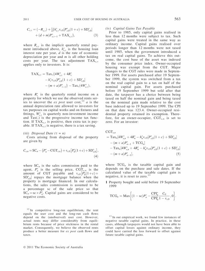
FIGURE 1Three-city Averages of the UCH, Housing Loan

Interest Rates and Property Price Growth

Notes: The ‘UCH: Average of 3 Cities · 8 Scenarios (% p.a.)’is the average of the 24 User Cost of Housing estimates(3 cities · 8 scenarios) for the 20 quarters beginning in thequarter indicated. The three cities are Brisbane, Melbourneand Sydney. The eight scenarios are defined in Section V.The ‘Housing Loan Interest Rate: 20 Qtr MA (% p.a.)’ is the20-quarter moving average of the standard variable homeloan interest rate (% p.a.) over the same holding period asthe UCH. The ‘3 City Ave of Quarterly Change in PropertyPrice: 20 Qtr MA’ is the 20-quarter moving average percent-age per annum growth rate in property prices. For each city,we calculate the proportional change in quarterly medianprice, DP = (Pt ) Pt)1) ⁄ Pt)1, as a percentage. At each t, wetake the average of the annualised DP across the three citiesand then take the 20-quarter moving average, over the sameholding period as the UCH.

2011 USER COST OF HOUSING IN AUSTRALIA 565

fittings (0.5 per cent per annum).16 Economicdepreciation is not deductible for tax purposes.Where the property purchase is supported by aloan, we assume that the loan-to-valuation ratiois 80 per cent and the loan is an interest-only loan.17 Agents’ sales commission is set at2 per cent of the selling price. Sensitivity analy-sis suggests that the tenor of the results is gen-erally not affected by the particular numbersassumed.

The relevant schedules of rates for Australianpersonal income tax (including tax on capitalgains), together with the relevant tax rules(including options held by taxpayers) wereobtained from the Australian Taxation Office.Further details are provided in the Appendix.We also obtained schedules of stamp duty onproperty transfers for New South Wales,Queensland and Victoria and the dates on whichthese schedules were changed from the respec-tive state revenue offices. Further details areprovided in the Appendix. We assume thatowner-occupiers take advantage of any owner-occupier concession but we exclude any furtherconcessions for first-home buyers and pension-ers. We also ignore first-home buyer grants,which in most cases were relatively small com-pared with the property price.

V ResultsThe UCH is estimated for Brisbane, Mel-

bourne and Sydney. For each city, we considereight scenarios, consisting of: 2 ownershipcategories (owner-occupier or investor) · 2 debtlevels (80 per cent debt or no debt) · 2 non-property income levels (average income or twiceaverage income). The holding period is 20 quar-ters (5 years).

16 Depending on the building’s construction date,the annual capital works allowance is 0, 2.5 or 4 percent of the construction cost. The annual depreciationrates for fixtures and fittings vary widely from item toitem and may be as high as 20 per cent. In all cases,these percentages apply to the original cost. Hence,these allowances as a percentage of the total propertyprice will be much lower than the percentages speci-fied in the tax rules, especially in the case of thepurchase of an established property.

17 Interest-only loans are not uncommon for inves-tors but are unusual for owner-occupiers. However, asthe loan-to-valuation ratio is 80 per cent, the amorti-sation rate would be low. Hence, it makes little differ-ence to assume that the loan is interest-only.

� 2011 The Economic Society of Australia

In Figure 1, we plot the average UCH acrossthe three cities and the eight scenarios.18 Theaverage UCH ranges from approximately )5 to15 per cent and trended downward until the late1990s and has since been on an upward path.The major drivers of the UCH are interest ratesand property price growth. Because the UCHdata have the character of a moving average, wealso plot interest rates and property price growthas moving averages. The contribution of interestrates has been treading steadily downwards overthe period, whereas the contribution of propertyprice growth has been volatile. In Figure 2, weprovide graphs of the ratio of median propertyprice to average annual earnings, which is asimpler measure of housing affordability. Asexpected, the UCH provides a very different

18 We recognise that the results reported for eachstart date are not independent because the estimationperiods overlap. Our objective here is simply tosummarise the findings.

0

0.2

0.4

0.6

0.8

1

1.2

1988

1989

1990

1991

1992

1993

1994

1995

1996

1997

1998

1999

2000

2001

2002

2003

2004

Interest payments/income: Brisbane Interest payments/income: Melbourne

Interest payments/income: Sydney

FIGURE 3The Ratio of Interest Payable to Income in Brisbane,

Melbourne and Sydney

Notes: ‘Interest Payments’ is the annual interest payable on aloan whose principal is equal to 80 per cent of the medianproperty price. Income is measured by annualised averageweekly earnings for each state.

0

2

4

6

8

10

12

1988

1989

1990

1991

1992

1993

1994

1995

1996

1997

1998

1999

2000

2001

2002

2003

2004

Property price/annualised AWE: Brisbane

Property price/annualised AWE: Melbourne

Property price/annualised AWE: Sydney

FIGURE 2The Ratio of Property Price to Income in Brisbane,

Melbourne and Sydney

Notes: The property price is the median price of three-bedroom houses in each of Brisbane, Melbourne and Sydney.Income is measured by annualised average weekly earningsfor each state.

566 ECONOMIC RECORD DECEMBER

picture to that provided by the alternative mea-sure. For example, while the UCH is falling formuch of the sample period, the ratio of prop-erty price to earnings is usually either flat orincreasing.

To enable some insight into the movement ofthe UCH over time, we provide in Figure 3plots of the ratio of annual interest payable toaverage annual earnings.

Interest rates were very high early in thesample period. The overall picture, therefore,

is clear: early in the period the UCH washigh because interest rates were high andprice appreciation was low. As these circum-stances reversed, the UCH fell steadily, reach-ing a minimum for the period starting in thelate 1990s. Since that period, the UCH hasrisen somewhat, but the rise has beenrestrained by the continuing low level of inter-est rates.

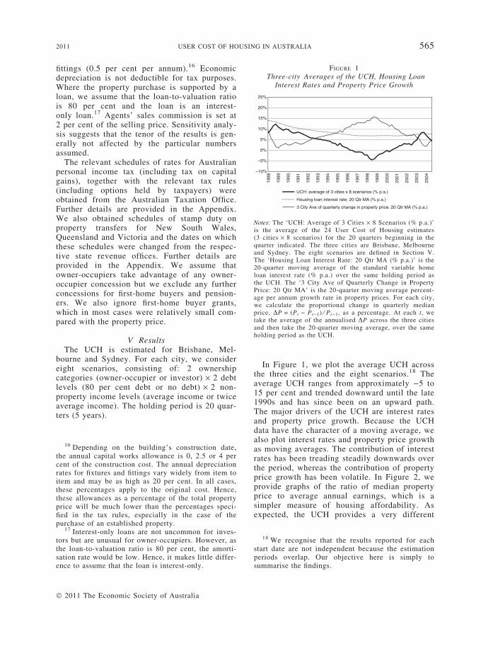
We now turn to the detailed results shown inTable 2 and Figure 4.

(i) Variation of the UCH Over TimeThe UCH varies considerably over time.

For Brisbane, the range is from )9.03 to10.29 per cent; for Melbourne, )5.47 to 15.17per cent and for Sydney, )6.97 to 18.84 percent. In every case, these minima wererecorded for the period from the late 1990s tothe early 2000s for owner-occupiers with‘high’ incomes and no debt. This period sawrelatively low interest rates and high priceappreciation. The maxima were also recordedby owner-occupiers but occurred in the early-to mid-1990s for those with debt and earn-ing only average incomes. This period sawrelatively high interest rates and low priceappreciation.

(ii) Variation of the UCH Between OwnerCategories

Variation in the UCH between owner cate-gories is considerably less than variation overtime. The eight scenarios we consider cover awide range of owners, including both tenuretypes, debt levels varying from 0 to 80 percent and non-property income being doubled.Yet, while there are exceptions, in many casesthe effect on the UCH is of the order of onlya few percentage points, especially in Mel-bourne and Sydney. In nearly every case, thelowest UCH is recorded by owner-occupierswho have no debt and who earn twice theaverage income. In every case, the highestUCH is recorded by property owners with debtand who earn the average income. Early andlate in the sample period, the highest UCHswere recorded by owner-occupiers; betweenthese periods, investors faced the higherUCH. Figure 4 depicts the upper and lowerboundaries of the UCH for Sydney. This figureillustrates clearly that the UCH between sce-narios is highly correlated, and that the vari-ability of the UCH over time is considerably

� 2011 The Economic Society of Australia

TABLE 2User Cost of Housing (UCH) – Classified by Time Period and Owner Attributes

Startdate

Investors Owner-occupiers

With debt No debt With debt No debt

Averageincome

Averageincome · 2

Averageincome

Averageincome · 2

Averageincome

Averageincome · 2

Averageincome

Averageincome · 2

Panel A: Brisbane1988 6.06 5.57 5.12 4.22 5.53 5.22 1.40 0.561989 7.63 7.11 6.18 5.80 8.43 8.20 3.71 2.971990 8.41 7.80 6.52 6.32 9.82 9.63 4.87 4.221991 8.66 8.00 6.67 6.05 10.09 9.93 5.35 4.741992 8.61 7.92 6.70 6.49 9.93 9.76 5.46 4.831993 8.96 8.27 7.27 7.02 10.11 9.96 6.03 5.401994 9.16 8.49 7.65 7.53 10.29 10.14 6.42 5.841995 8.72 8.17 7.37 7.09 9.60 9.48 6.00 5.511996 7.11 6.77 5.97 6.16 7.46 7.33 4.24 3.761997 4.78 4.47 3.71 3.94 4.40 4.23 1.37 0.861998 )0.55 )0.95 )1.56 )0.85 )2.62 )2.90 )5.38 )6.011999 )3.12 )3.57 )4.03 )4.48 )5.83 )6.19 )8.28 )9.032000 )2.21 )2.63 )3.01 )3.37 )4.41 )4.75 )6.54 )7.302001 )1.32 )1.74 )2.09 )2.56 )2.89 )3.20 )4.87 )5.562002 )0.81 )1.28 )1.60 )1.82 )1.96 )2.24 )4.02 )4.682003 2.32 1.73 1.38 )0.03 2.13 1.89 )0.40 )1.082004 4.74 4.08 3.55 3.28 5.18 5.00 2.26 1.64

Panel B: Melbourne1988 9.22 8.18 7.87 6.97 11.95 11.68 7.06 6.161989 12.17 11.01 10.14 9.65 15.07 14.85 9.45 8.631990 12.49 11.50 10.19 9.89 15.17 15.01 9.56 8.871991 10.09 9.24 7.93 8.02 12.40 12.24 7.29 6.661992 7.34 6.62 5.43 5.22 8.70 8.53 4.12 3.531993 6.20 5.55 4.56 4.24 6.54 6.37 2.44 1.911994 4.05 3.49 2.70 2.86 3.13 2.97 )0.49 )0.961995 1.11 0.79 0.07 0.24 0.43 0.30 )2.60 )2.961996 )1.21 )1.51 )2.09 )2.22 )2.49 )2.67 )5.08 )5.471997 )0.66 )1.14 )1.55 )2.21 )1.73 )1.95 )4.18 )4.641998 )0.77 )1.39 )1.65 )2.07 )1.79 )2.04 )4.13 )4.681999 1.87 1.14 0.96 0.06 1.82 1.58 )0.57 )1.202000 3.67 2.91 2.78 1.99 4.25 4.02 1.91 1.242001 5.64 4.75 4.57 3.79 6.86 6.65 4.27 3.572002 5.65 4.71 4.52 4.28 6.96 6.74 4.16 3.422003 7.65 6.66 6.39 5.13 9.45 9.25 6.32 5.582004 6.34 5.49 5.03 5.18 7.77 7.59 4.64 3.99

Panel C: Sydney1988 14.73 13.18 12.77 10.43 17.83 17.60 12.07 11.081989 15.64 14.05 13.07 13.43 18.84 18.63 12.40 11.481990 9.72 8.76 7.54 7.49 12.17 12.00 6.83 6.171991 8.72 7.86 6.50 6.32 11.07 10.93 5.91 5.391992 6.51 5.87 4.63 4.35 7.64 7.51 3.10 2.681993 4.90 4.30 3.31 3.14 4.58 4.46 0.67 0.311994 4.04 3.48 2.64 2.67 3.57 3.47 )0.04 )0.341995 1.96 1.56 0.79 0.89 1.91 1.81 )1.30 )1.541996 0.11 )0.31 )0.84 )0.92 )0.48 )0.64 )3.21 )3.581997 )1.94 )2.49 )2.85 )3.11 )3.16 )3.38 )5.67 )6.14

2011 USER COST OF HOUSING IN AUSTRALIA 567

� 2011 The Economic Society of Australia

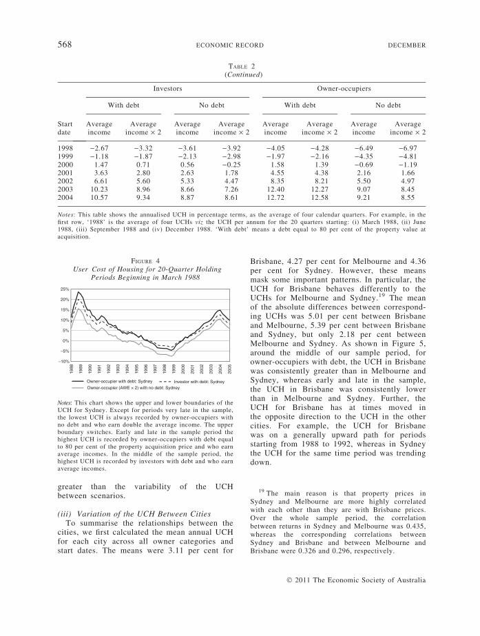
TABLE 2(Continued)

Startdate

Investors Owner-occupiers

With debt No debt With debt No debt

Averageincome

Averageincome · 2

Averageincome

Averageincome · 2

Averageincome

Averageincome · 2

Averageincome

Averageincome · 2

1998 )2.67 )3.32 )3.61 )3.92 )4.05 )4.28 )6.49 )6.971999 )1.18 )1.87 )2.13 )2.98 )1.97 )2.16 )4.35 )4.812000 1.47 0.71 0.56 )0.25 1.58 1.39 )0.69 )1.192001 3.63 2.80 2.63 1.78 4.55 4.38 2.16 1.662002 6.61 5.60 5.33 4.47 8.35 8.21 5.50 4.972003 10.23 8.96 8.66 7.26 12.40 12.27 9.07 8.452004 10.57 9.34 8.87 8.61 12.72 12.58 9.21 8.55

Notes: This table shows the annualised UCH in percentage terms, as the average of four calendar quarters. For example, in thefirst row, ‘1988’ is the average of four UCHs viz the UCH per annum for the 20 quarters starting: (i) March 1988, (ii) June1988, (iii) September 1988 and (iv) December 1988. ‘With debt’ means a debt equal to 80 per cent of the property value atacquisition.

–10%

–5%

0%

5%

10%

15%

20%

25%

1988

1989

1990

1991

1992

1993

1994

1995

1996

1997

1998

1999

2000

2001

2002

2003

2004

2005

Owner-occupier with debt: Sydney Investor with debt: SydneyOwner-occupier (AWE × 2) with no debt: Sydney

FIGURE 4User Cost of Housing for 20-Quarter Holding

Periods Beginning in March 1988

Notes: This chart shows the upper and lower boundaries of theUCH for Sydney. Except for periods very late in the sample,the lowest UCH is always recorded by owner-occupiers withno debt and who earn double the average income. The upperboundary switches. Early and late in the sample period thehighest UCH is recorded by owner-occupiers with debt equalto 80 per cent of the property acquisition price and who earnaverage incomes. In the middle of the sample period, thehighest UCH is recorded by investors with debt and who earnaverage incomes.

19 The main reason is that property prices inSydney and Melbourne are more highly correlatedwith each other than they are with Brisbane prices.Over the whole sample period, the correlationbetween returns in Sydney and Melbourne was 0.435,whereas the corresponding correlations betweenSydney and Brisbane and between Melbourne andBrisbane were 0.326 and 0.296, respectively.

568 ECONOMIC RECORD DECEMBER

greater than the variability of the UCHbetween scenarios.

(iii) Variation of the UCH Between CitiesTo summarise the relationships between the

cities, we first calculated the mean annual UCHfor each city across all owner categories andstart dates. The means were 3.11 per cent for

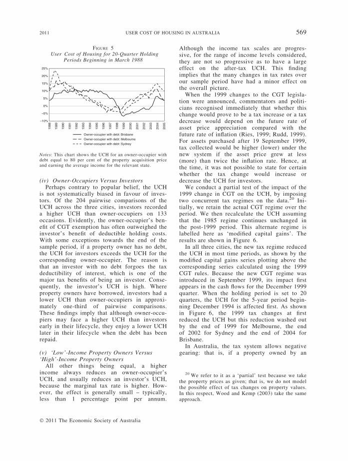
Brisbane, 4.27 per cent for Melbourne and 4.36per cent for Sydney. However, these meansmask some important patterns. In particular, theUCH for Brisbane behaves differently to theUCHs for Melbourne and Sydney.19 The meanof the absolute differences between correspond-ing UCHs was 5.01 per cent between Brisbaneand Melbourne, 5.39 per cent between Brisbaneand Sydney, but only 2.18 per cent betweenMelbourne and Sydney. As shown in Figure 5,around the middle of our sample period, forowner-occupiers with debt, the UCH in Brisbanewas consistently greater than in Melbourne andSydney, whereas early and late in the sample,the UCH in Brisbane was consistently lowerthan in Melbourne and Sydney. Further, theUCH for Brisbane has at times moved inthe opposite direction to the UCH in the othercities. For example, the UCH for Brisbanewas on a generally upward path for periodsstarting from 1988 to 1992, whereas in Sydneythe UCH for the same time period was trendingdown.

� 2011 The Economic Society of Australia

–10%

–5%

0%

5%

10%

15%

20%

25%

1988

1989

1990

1991

1992

1993

1994

1995

1996

1997

1998

1999

2000

2001

2002

2003

2004

2005

Owner-occupier with debt: Brisbane

Owner-occupier with debt: Melbourne

Owner-occupier with debt: Sydney

FIGURE 5User Cost of Housing for 20-Quarter Holding

Periods Beginning in March 1988

Notes: This chart shows the UCH for an owner-occupier withdebt equal to 80 per cent of the property acquisition priceand earning the average income for the relevant state.

20 We refer to it as a ‘partial’ test because we takethe property prices as given; that is, we do not modelthe possible effect of tax changes on property values.In this respect, Wood and Kemp (2003) take the sameapproach.

2011 USER COST OF HOUSING IN AUSTRALIA 569

(iv) Owner-Occupiers Versus InvestorsPerhaps contrary to popular belief, the UCH

is not systematically biased in favour of inves-tors. Of the 204 pairwise comparisons of theUCH across the three cities, investors recordeda higher UCH than owner-occupiers on 133occasions. Evidently, the owner-occupier’s ben-efit of CGT exemption has often outweighed theinvestor’s benefit of deductible holding costs.With some exceptions towards the end of thesample period, if a property owner has no debt,the UCH for investors exceeds the UCH for thecorresponding owner-occupier. The reason isthat an investor with no debt forgoes the taxdeductibility of interest, which is one of themajor tax benefits of being an investor. Conse-quently, the investor’s UCH is high. Whereproperty owners have borrowed, investors had alower UCH than owner-occupiers in approxi-mately one-third of pairwise comparisons.These findings imply that although owner-occu-piers may face a higher UCH than investorsearly in their lifecycle, they enjoy a lower UCHlater in their lifecycle when the debt has beenrepaid.

(v) ‘Low’-Income Property Owners Versus‘High’-Income Property Owners

All other things being equal, a higherincome always reduces an owner-occupier’sUCH, and usually reduces an investor’s UCH,because the marginal tax rate is higher. How-ever, the effect is generally small – typically,less than 1 percentage point per annum.

� 2011 The Economic Society of Australia

Although the income tax scales are progres-sive, for the range of income levels considered,they are not so progressive as to have a largeeffect on the after-tax UCH. This findingimplies that the many changes in tax rates overour sample period have had a minor effect onthe overall picture.

When the 1999 changes to the CGT legisla-tion were announced, commentators and politi-cians recognised immediately that whether thischange would prove to be a tax increase or a taxdecrease would depend on the future rate ofasset price appreciation compared with thefuture rate of inflation (Ries, 1999; Rudd, 1999).For assets purchased after 19 September 1999,tax collected would be higher (lower) under thenew system if the asset price grew at less(more) than twice the inflation rate. Hence, atthe time, it was not possible to state for certainwhether the tax change would increase ordecrease the UCH for investors.

We conduct a partial test of the impact of the1999 change in CGT on the UCH, by imposingtwo concurrent tax regimes on the data.20 Ini-tially, we retain the actual CGT regime over theperiod. We then recalculate the UCH assumingthat the 1985 regime continues unchanged inthe post-1999 period. This alternate regime islabelled here as ‘modified capital gains’. Theresults are shown in Figure 6.

In all three cities, the new tax regime reducedthe UCH in most time periods, as shown by themodified capital gains series plotting above thecorresponding series calculated using the 1999CGT rules. Because the new CGT regime wasintroduced in September 1999, its impact firstappears in the cash flows for the December 1999quarter. When the holding period is set to 20quarters, the UCH for the 5-year period begin-ning December 1994 is affected first. As shownin Figure 6, the 1999 tax changes at firstreduced the UCH but this reduction washed outby the end of 1999 for Melbourne, the endof 2002 for Sydney and the end of 2004 forBrisbane.

In Australia, the tax system allows negativegearing: that is, if a property owned by an

–5%

0%

5%

10%

15%

20%

1988

1989

1990

1991

1992

1993

1994

1995

1996

1997

1998

1999

2000

2001

2002

2003

2004

2005

Investor: Brisbane Investor (modified capital gains): Brisbane

Investor: Melbourne Investor (modified capital gains): Melbourne

Investor: Sydney Investor (modified capital gains): Sydney

FIGURE 6The Effect of the 1999 Change in Capital Gains

Tax (CGT) on the User Cost of Housing (UCH) forInvestors

Notes: The property investor has a debt equal to 80 per centof the property acquisition price. ‘Modified capital gains’means that the UCH is estimated assuming that the 1985CGT regime continues beyond 1999.

–1%

0%

1%

2%

3%

4%

5%

6%

1988

1989

1990

1991

1992

1993

1994

1995

1996

1997

1998

1999

2000

2001

2002

2003

2004

2005

Investor with debt – NGP:Sydney

Investor with no debt – NGP:Sydney

Investor (AWE × 2) with debt – NGP:Sydney

Investor (AWE × 2) with no debt – NGP:Sydney

FIGURE 7The Negative Gearing Premium for Investors

Notes: ‘NGP’ is the negative gearing premium and is calcu-lated as the UCH if negative gearing is not permitted for taxpurposes less the UCH with full negative gearing permitted(as calculated previously). ‘With debt’ indicates that theowner has a debt equal to 80 per cent of the property acqui-sition price. ‘Investor’ means an investor earning the averageincome. ‘Investor (AWE · 2)’ means an investor earningdouble the average income. The city is Sydney.

570 ECONOMIC RECORD DECEMBER

investor generates a loss, this loss can be fullyoffset against other sources of income.21 Thisfeature of the tax system has generated consid-erable public discussion, much of it critical. Forexample, Tim Colebatch, the economics editorof The Age (Melbourne), wrote in that newspa-per on 30 March 2010:

In one swoop it [the government] shouldremove the two big tax distortions of the mar-ket. End the exemption of the family homefrom capital gains tax. End the tax break fornegative gearing … On average, in 2007-08,they [negatively geared investors] claimedlosses of more than $200 a week on theirproperties. This gave them a tax break ofabout $5 billion that year … As public policy,this is ridiculous.

Wood and Kemp’s (2003) study simulated theeffect of adopting British tax laws in Australiaand suggested that the effect of the less gener-ous British rules on negative gearing in Austra-lia would be limited. Being a simulation study,Wood and Kemp (2003) cannot – and did notintend to – provide an estimate of the effect thatthe negative gearing rules have in fact had.

21 The Productivity Commission (2004, pp. 76–7)reports that 17 per cent of taxpayers report rentalincome, of whom approximately 40 per cent report anet loss on the investment.

Accordingly, we re-estimate the user cost forinvestors, assuming that losses were not deduct-ible at all; this is a particularly harsh tax treat-ment because it eliminates even the carryingforward of losses. We refer to the differencebetween this user cost and the actual user costcalculated previously as the ‘negative gearingpremium’. In effect, this premium is a measureof the reduction in the user cost that the currenttax rules permit, relative to a tax rule that elimi-nates all tax benefits associated with negativegearing. For illustrative purposes, we provide inFigure 7 the negative gearing premium for vari-ous categories of Sydney investors.

In all three cities, the negative gearing pre-mium for investors with debt was highest earlyin our sample period, when interest rates wereparticularly high. The premium then fell for adecade or more, with some increase in recentyears, followed by a further fall. Across thethree cities, the mean premium for investorswith debt was 1.75 per cent per annum for thoseearning the mean income and 2.42 per cent perannum for those earning twice the mean income.This greater benefit is of course due to thehigher tax rate faced by higher income earn-ers. There are, however, important differencesbetween the cities. In Brisbane, the negativegearing premium for investors with debt variesfrom approximately 0.8 per cent per annum to

� 2011 The Economic Society of Australia

–1%

0%

1%

2%

3%

4%

1988

1989

1990

1991

1992

1993

1994

1995

1996

1997

1998

1999

2000

2001

2002

2003

2004

2005

Investor with debt -GTF: Brisbane Investor with debt -GTF: Melbourne

Investor with debt -GTF: Sydney

FIGURE 8The User Cost of Housing (UCH) After Eliminating

the 50 Per Cent Discount in Capital Gains Taxation

Notes: The figure shows the effect of eliminating the 50 percent discount on capital gains tax, which is calculated as theUCH if capital gains are fully taxable less the UCH withonly 50 per cent of capital gains being taxable (as calculatedpreviously). The investor has a debt equal to 80 per cent ofthe property acquisition price. ‘GTF’ signifies that the fullamount of the capital gain is taxable.

2011 USER COST OF HOUSING IN AUSTRALIA 571

2.3 per cent per annum, depending on the timeperiod and the investor’s income. The findingsfor Melbourne and Sydney are quite similar toeach other, but the premiums are generallyhigher than those found for Brisbane investors.Except for a spike in the early years of our sam-ple period, the negative gearing premium inboth Melbourne and Sydney varies from around1.5 per cent per annum to approximately 3 or3.5 per cent per annum. In general, the negativegearing premium for Sydney is slightly greaterthan for Melbourne, which in turn is clearlygreater than for Brisbane. For investors earningthe average income, the mean annual premiumis 1.37 per cent in Brisbane, 1.88 per cent inMelbourne and 2.00 per cent in Sydney.Towards the end of the sample period, there is asmall negative gearing premium for investorswho have no debt: non-interest holding costswere sufficiently high that even in the absenceof interest costs the tax treatment of negativegearing was beneficial to investors.

The 1999 changes to CGT included a ‘dis-count’ of 50 per cent: only half of a nominalcapital gain was to be taxed. The choice of 50per cent is essentially arbitrary. It can be arguedthat if a capital gain is income then all of thegain should be subject to income tax. Indeed,the Australian tax system treats capital gainsmade in less than 12 months in exactly thisfashion. Arguably, therefore, the CGT discountis a distortion that reduces the UCH forinvestors.22

To estimate the extent of this distortion, were-calculate the UCH for investors with the dis-count eliminated but we retain the taxpayer’soption to choose the frozen indexation method.We then calculate the change in the UCHcaused by the elimination of the discount. Theresults are shown in Figure 8.

In all three cities, there is a substantialincrease in the UCH for 5-year holding periodsbeginning in 1995, reaching a peak of between3 and 3.7 per cent after 3–5 years. In all threecities, the effect then declines.23

22 Of course, the CGT exemption (equivalent to adiscount of 100 per cent) for owner-occupiers can beseen as an even greater distortion.

23 As a robustness check, we also modelled theeffect of simultaneously eliminating both the CGTdiscount and the transitional frozen indexationmethod. The result is a further increase in the UCH,but the size of this increase is very small.

� 2011 The Economic Society of Australia

In Brisbane, the CGT discount effect forinvestors with debt is generally greater than thenegative gearing effect. In Melbourne and Syd-ney, the comparison is more complex. Untilabout 1999, the CGT effect exceeds the negativegearing effect, but thereafter the reverse is true.Across the three cities, for investors earningaverage incomes, the mean annual CGT effect is1.57 per cent, as against a mean annual negativegearing premium of 1.50 per cent. However, anassessment of the relative effects of the two taxtreatments also needs to take into account thefact that the negative gearing rules have thegreatest effect on those investors who haveborrowed, whereas the CGT discount applies toall investors who are taxpayers. For investorswithout debt, the CGT effect far exceeds thenegative gearing effect. We conclude that thedistorting effects of the CGT discount are atleast as worthy of public discussion as thealleged distorting effects of negative gearing.

VI Policy DiscussionEnglund (2003) characterises the two modes

of tenure (tenant and owner-occupier) as alter-native technologies that can be used to producethe same output (housing services). Seen in thislight, the principle of production efficiency –that the tax system should not affect the choice

572 ECONOMIC RECORD DECEMBER

of production method – implies that the tax sys-tem should not systematically favour one formof tenure over the other. That is, there needs tobe tax neutrality. He reviews the main featuresof the tax systems of 16 OECD countries andfinds that only six do not levy any form of CGTon owner-occupiers and only one does notprovide any form of interest deductibility forowner-occupiers. As he succinctly states, ‘Inmost countries, owner-occupancy tends to befavoured [by the tax system] relative to renting’(Englund, 2003, p. 938). Given that investorsalso are taxed on capital gains and are entitledto interest deductibility, Englund identifies themain tax difference to be the fact that investorsare taxed on rent received, but owner-occupiersare not taxed on their imputed rent. Consistentwith this analysis, his main policy recommenda-tion is an annual property tax on owner-occupi-ers to proxy for a tax on imputed rent.

Although Englund’s framework provides auseful way to think about tax and tenure choice,his particular recommendation is not necessarilytransferable to Australian conditions. Unlike theOECD countries he surveyed, Australia does notlevy CGT on owner-occupiers but neither doesit allow them deductibility for interest paymentsor other property holding costs. Consequently,a tax on imputed rent is needed for productionefficiency only to the extent that the owner-occupier’s CGT exemption is less valuable thanthe investor’s right to tax deductibility of inter-est payments and other holding costs. The evi-dence we provide suggests that, over the past20 years, on balance, the system tends to favourowner-occupiers over investors. That is, in gen-eral, the CGT exemption is more valuable thanthe deductibility of holding costs, especially forproperty owners with no debt. Our evidence alsosuggests that the focus of some commentatorson the alleged distortion of negative gearing ismisplaced. If it is a distortion, it is of a similarorder of magnitude to the distortion of the largeCGT discounts available to property owners:50 per cent in the case of investors and 100 percent in the case of owner-occupiers. We alsoobserve that the tax treatment of negative gear-ing is entirely consistent with the tax treatmentof reductions to income brought about by othercircumstances, such as investments in equities.But the CGT discounts are inconsistent with thetreatment of other forms of income and, in par-ticular, with the tax treatment of capital gainsmade in a period of less than 12 months.

However, the main policy implication of ourresults is that in practice tax policy has been farless important than interest rate policy. Wheninterest rates are high – as in the early 1990s forexample – the UCH is also high for both inves-tors and owner-occupiers. The magnitude of thiseffect easily exceeds the magnitude of the effectof differences in the tax treatment of investorsand owner-occupiers.

VII ConclusionWe estimate the ex post UCH in Brisbane,

Melbourne and Sydney in the period from 1988to 2010. We find that the UCH varied consider-ably over time, from )9 per cent to more than18 per cent depending on the city, the time per-iod, the level of debt and the ownership cate-gory. By comparison, the variation betweenownership categories is typically much smaller,and is often only a few percentage pointsdespite great differences in indebtedness,income levels and tax rates. Despite the tax ben-efits conferred on investors, the UCH is oftenlower for owner-occupiers than investors. Essen-tially, this finding implies that the owner-occu-piers’ benefit of exemption from CGT oftenoutweighs the investors’ benefit from thedeductibility of holding costs. The negativegearing tax rules have delivered benefits toinvestors with debt, typically of the order of1.5–3.5 per cent per annum, but going as highas 5 per cent per annum in the period wheninterest rates were very high. The CGT changesintroduced in 1999 benefited investors eventhough, in principle, these changes might haveimposed a greater tax burden than the system itreplaced. Finally, the popular ire towards nega-tive gearing would be better directed towardsCGT rules.

Supporting InformationAdditional Supporting Information may be

found in the online version of this article:DATA S1 Datasets and CodesPlease note: Wiley-Blackwell is not responsible

for the content or functionality of any supportingmaterials supplied by the authors. Any queries(other than missing material) should be directedto the corresponding author for the article.

REFERENCES

Abelson, P. (2009), ‘Affordable Housing: Conceptsand Policy’, Economic Papers, 28, 27–38.

� 2011 The Economic Society of Australia

2011 USER COST OF HOUSING IN AUSTRALIA 573

Abelson, P. and Joyeux, R. (2007), ‘Price and Effi-ciency Effects of Taxes and Subsidies for Austra-lian Housing’, Economic Papers, 26, 147–69.

Baldwin, A., Nakamura, A.O. and Prud’homme, M.(2009), ‘Different Concepts for Measuring OwnerOccupied Housing Costs in a CPI: Statistics Can-ada’s Analytical Series’, in Diewert, W.E., Balk,B.M., Fixler, D., Fox, K.J. and Nakamura, A.O.(eds), Price and Productivity Measurement: Volume1 – Housing. Trafford Press. Available from: http://www.indexmeasures.com/V1_FCh10_2009_03_04_Baldwin_ANakamura_Prudhomme.pdf.

Barham, G. (2004), ‘The Effects of Taxation Policyon the Cost of Capital in Housing – A HistoricalProfile’, Financial Stability Report, Central Bank ofIreland, Dublin 2, Ireland, 89–102.

Bostic, R., Gabriel, S. and Painter, G. (2008), ‘Hous-ing Wealth, Financial Wealth, and Consumption:New Evidence From Micro Data’, Lusk Centre forReal Estate Working Paper No. 2008-1006, Univer-sity of Southern California, Los Angeles.

Canner, G., Dynan, K. and Passmore, W. (2002),‘Mortgage Refinancing in 2001 and Early 2002’,Federal Reserve Bulletin, 88 (December), 469–81.

Chow, Y.F. and Wong, N. (2003), ‘Property Value,User Cost and Rent: An Investigation of the Resi-dential Property Market in Hong Kong’, Journal ofBusiness and Economics Research, 1, 9–17.

Colebatch, T. (2010), ‘Caught in the Cogs of the TaxRegime’, The Age, 30 March.

Diewert, W.E. (2004), ‘The Treatment of OwnerOccupied Housing and Other Durables in a Con-sumer Price Index’, Centre for Applied EconomicResearch Working Paper No. 2004 ⁄ 3, University ofNew South Wales, Sydney.

Dvornak, N. and Kohler, M. (2003), ‘Housing Wealth,Stock Market Wealth and Consumption: A PanelAnalysis for Australia’, Reserve Bank of AustraliaResearch Discussion Paper No. 2003-7, RBA, Sydney.

Englund, P. (2003), ‘Taxing Residential HousingCapital’, Urban Studies, 40, 937–52.

Fane, G. and Richardson, M. (2005), ‘Negative Gear-ing and the Taxation of Capital Gains in Australia’,Economic Record, 81, 249–61.

Garner, C.A. (1992), ‘Will the Real Price of Hous-ing Drop Sharply in the 1990s?’, Economic Review,Federal Reserve Bank of Kansas City, 1st Qtr, 55–64.

Gervais, M. and Pandey, M. (2008), ‘Who CaresAbout Mortgage Interest Deductibility?’, CanadianPublic Policy, 34, 1–24.

Gillingham, R. (1980), ‘Estimating the User Cost ofOwner-Occupied Housing’, Monthly Labor Review,103, 31–5.

Greenspan, A. and Kennedy, J. (2005), Estimates ofHome Mortgage Originations, Repayments, andDebt on One-to-Four-Family Residences, Financeand Economics Discussion Series 2005-411, Boardof Governors of the Federal Reserve System, Wash-ington, D.C.

� 2011 The Economic Society of Australia

Guðnason, R. (2004), ‘Simple User Cost and Rentals’,8th meeting of the International Working Group onPrice Indices (The Ottawa Group), Helsinki, 23–25August.

Hendershott, P.H. and Slemrod, J. (1983), ‘Taxes andthe User Cost of Capital for Owner-Occupied Hous-ing’, AREUEA Journal, 10, 375–93.

Hennessey, S.M. (2003), ‘The Impact of HousingChoice on Future Household Wealth’, FinancialServices Review, 12, 143–64.

Himmelberg, C., Mayer, C. and Sinai, T. (2005),‘Assessing High House Prices: Bubbles, Funda-mentals and Misperceptions’, Journal of EconomicPerspectives, 19, 67–92.

International Labour Office (2004), The ConsumerPrice Index Manual: Theory and Practice. Interna-tional Labour Office, Geneva.

Jorgenson, D.W. (1963), ‘Capital Theory and Invest-ment Behavior’, American Economic Review, 53,247–59.

Lee, T.H. and Chung, K.J. (1997), ‘Measuring theUser Cost of Owner-Occupied Housing for theTrue Cost of Living Index’, International EconomicJournal, 11, 1–14.

Manchester, J.M. and Poterba, J.M. (1989), ‘SecondMortgages and Household Saving’, Regional Scienceand Urban Economics, 19, 325–46.

Miles, D. (1994), Housing, Financial Markets and theWider Economy. John Wiley and Sons, New York.

Poole, R., Ptacek, F. and Verbrugge, R. (2005), Treat-ment of Owner-Occupied Housing in the CPI.Office of Prices and Living Conditions, Bureau ofLabor Statistics, Washington.

Poterba, J.M. (1984), ‘Tax Subsidies to Owner-Occupied Housing: An Asset-Market Approach’,Quarterly Journal of Economics, 99, 729–52.

Poterba, J.M. and Sinai, T.M. (2008), ‘Income Tax Pro-visions Affecting Owner-Occupied Housing: Reve-nue Costs and Incentive Effects’, National Bureau ofEconomic Research Working Paper No. WP14253,NBER, Cambridge, MA.

Productivity Commission (2004), First Home Owner-ship, Report 28. Productivity Commission, Mel-bourne.

Ries, I. (1999), ‘Ralph’s Investment Wheel of Fortune’,Australian Financial Review, 25 September, 25–6.

Rudd, K. (1999), Commonwealth of Australia, Houseof Representatives Official Hansard, 11 October,Canberra, 11258–61.

Verbrugge, R. (2006), ‘The Puzzling Divergence ofRents and User Costs 1980–2004’, OECD-IMFworkshop, 6–7 November, Paris.

Wood, G.A. and Kemp, P.A. (2003), ‘The Taxation ofAustralian Landlords: Would the British Tax Treat-ment of Rental Investments Increase Tax Burdensif Introduced in Australia?’, Urban Studies, 40,747–65.

Woolford, K. (2006), ‘An Exploration of Alter-native Treatments of Owner-Occupied Housing in

574 ECONOMIC RECORD DECEMBER

a CPI’, OECD-IMF workshop, 6–7 November,Paris.

Yang, J. and Adams, F.G. (1994), ‘The User CostEstimation of Owner-Occupied Housing’, Journal ofPolicy Modeling, 16, 327–33.

Yates, J. and Bradbury, B. (2010), ‘Home Ownershipas a (Crumbling) Fourth Pillar in Social Insurancein Australia’, Journal of Housing and the Built Envi-ronment, 25, 193–211.

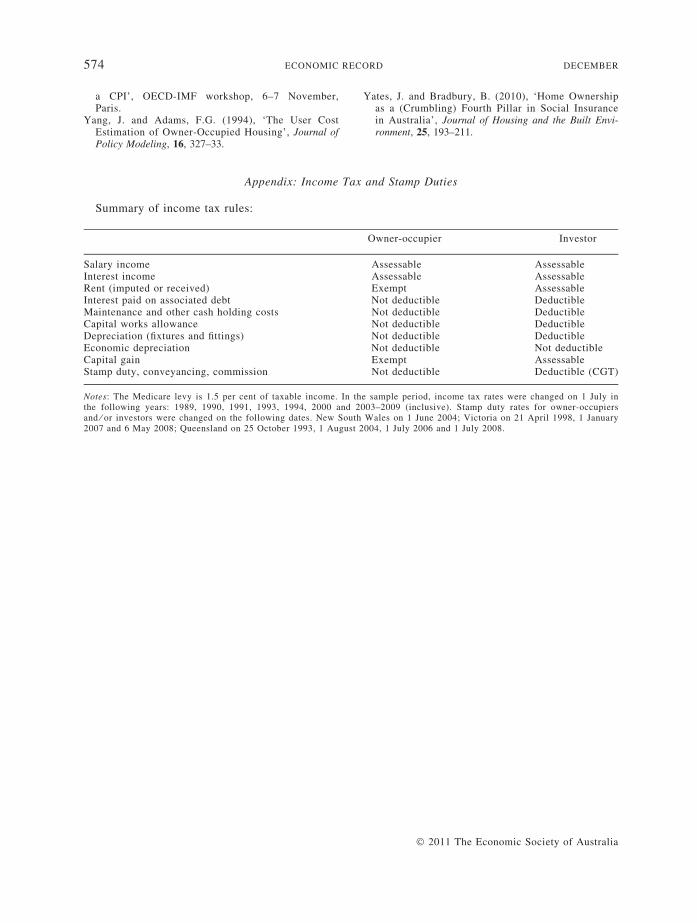
Appendix: Income Tax and Stamp Duties

Summary of income tax rules:

O

wner-occupier

� 2011 The Economic S

Investor

Salary income

Assessable Assessable Interest income Assessable Assessable Rent (imputed or received) Exempt Assessable Interest paid on associated debt Not deductible Deductible Maintenance and other cash holding costs Not deductible Deductible Capital works allowance Not deductible Deductible Depreciation (fixtures and fittings) Not deductible Deductible Economic depreciation Not deductible Not deductible Capital gain Exempt Assessable Stamp duty, conveyancing, commission Not deductible Deductible (CGT)

Notes: The Medicare levy is 1.5 per cent of taxable income. In the sample period, income tax rates were changed on 1 July inthe following years: 1989, 1990, 1991, 1993, 1994, 2000 and 2003–2009 (inclusive). Stamp duty rates for owner-occupiersand ⁄ or investors were changed on the following dates. New South Wales on 1 June 2004; Victoria on 21 April 1998, 1 January2007 and 6 May 2008; Queensland on 25 October 1993, 1 August 2004, 1 July 2006 and 1 July 2008.

ociety of Australia