Structure factor calculations for a side-by-side model of B-DNA

Structure factor calculations for a side-by-side model of B - D N A

S. R. Hubbard, R. J. Greenal l * Department of Physics, University of York, York YO 1 5DD, UK

A. K. Shrive, V. T. Forsyth and A. Mahendras ingam Department of Physics, University of Keele, Staffordshire ST5 5BG, UK

Received 22 February 1994; revised 27 May 1994

In this paper, the side-by-side model of DNA proposed by Premilat and Albiser is investigated. The axial repeat of the model is equal to the c-axis repeat in the observed B-DNA unit cell in fibres. However, the model does not pack into the unit cell as efficiently as the B-DNA double helix does, nor is it as successful as the double helix in predicting the observed Bragg amplitudes. When the azimuthal orientations and the relative axial displacements of the two molecules in the unit cell are allowed to take general values, the best crystallographic R factor for the side-by-side model is 43.43% compared with 34.33% for the double helix. If constraints consistent with the accepted B-DNA space group, P21212~, are applied, the best R factors are 45.53% for the side-by-side model and 34.51% for the double helix. Therefore, the side-by-side model can be rejected as a possible conformation for B-DNA in crystalline fibres.

Keywords: DNA double helical model; DNA side-by-side model; X-ray fibre diffraction

Although the double helical (DH) Watson-Crick ~ model for DNA is well established, alternative models have been proposed from time to time. In particular, the side-by-side (SBS) models have been extensively investigated 2-~°. In these models, the two polynucleotide chains are antiparallel and are linked by complementary Watson- Crick base pairs. The key characteristic of these models is that the molecule consists of alternating segments of right- and left-handed helix, each segment being about five nucleotide pairs in length.

Until recently, the sole direct evidence for the structure of DNA came from fibre diffraction, and, indeed, this technique is still the only means of visualizing the conformation of polymeric DNA. In the case of B-DNA, fibre diffraction can be particularly powerful, since the fibres frequently contain regions of high crystallinity. The diffraction pattern contains discrete Bragg reflections which give three-dimensional information about the molecular structure ~ L12. The confidence we may have in such models is comparable to that which we may have in structures derived from crystallographic studies on DNA fragments ~3. Unfortunately, the majority of the SBS models proposed so far have a long-range twist associated with them, giving a helical structure whose pitch is approximately ten times greater than the pitch of DH B-DNA. Therefore, these models will not fit into

* To whom correspondence should be addressed

the observed unit cell of B-DNA, and can clearly be rejected as possible conformations for the crystalline form. However, B-DNA has also been observed in semi-crystalline fibres and in even less ordered forms, in which case the observed diffraction is related to the cylindrically averaged squared transform (CAST) of an individual molecule. All the proposers of SBS models have suggested that their models are superior to the double helix when calculated CASTs are compared with observed intensities from disordered specimens. This view has been challenged ~4 17, and the point has been made that any model for DNA should be tested against the high-quality crystalline diffraction data. The reasoning behind this has been discussed extensively elsewhere la.

The proposal of an SBS model with no long-range twist by Premilat and Albiser 1° provides the first opportunity to calculate structure factors and to compare them with observed Bragg reflection amplitudes. In this paper, we report such calculations together with an investigation of the stereochemical feasibility of the model.

Methods

We have adopted the nucleotide naming convention that is customary for SBS models (Table 1). Premilat and Albiser ~ o have given the sugar and phosphate coordinates for residues A02 to A10. The coordinates for residue A01 were generated from those of A02 by application of the helix rise and rotation parameters of DH B-DNA

0141-8130/94/040195-11 :~ 1994 Butterworth-Heinemann Limited Int. J. Biol. Macromol. Volume 16 Number 4 1994 195

determined from fibre diffraction ~9. Coordinates for atoms in the B-chain were generated using the diad axis which is perpendicular to the molecular axis in nucleotide pairs 1 and 6. Premilat and Albiser gave the coordinates of the nitrogen atom attached to CI' in each nucleotide but none of the other base atoms, so these must be derived. The coordinates of a standard untilted and untwisted Watson-Crick base pair 17 were rotated and translated until the vector from the purine N9 to the pyrimidine N1 coincided with the vector from the A-chain nitrogen to the B-chain nitrogen. The pseudodiad axis in the plane of the base pair was maintained perpendicular to the molecular axis. Since all the nucleotides are in the anti conformation, it was necessary to invert the base pairs in nucleotides 4-8, which lie in the left-handed region of the molecule. The base sequence (Table 1) and the choice of zero propeller twist are arbitrary and unlikely to have a significant effect on the calculations reported here. Coordinates for a DH B-DNA molecule with the same base sequence were derived from the fibre model described by Arnott and Hukins x9. Views of the two models are shown in Figure 1. To check the acceptability of the intramolecular stereochemistry, bond lengths and bond angles were calculated, and short van der Waals' contacts were located. A short contact is defined as one

Table 1 Sequence of bases used in the ten nucleotide repeat unit

A-strand B-strand

3 p 5 '

A01 A T B01 A02 G - - C B02 A03 C G B03 A04 T - - A B04 A05 C - - G B05 A06 T A B06 A07 G - - C B07 A08 A T B08 A09 T A B09 A10 C G B10 5' 3'

A = adenine; T = thymine; G = guanine; C = cytosine

(a)

in which the distance between two atoms is less than the sum of their van der Waals' radii. The van der Waals' radii were taken to be 1.4 ,~ for O, 1.5 ,~ for N, 1.6 A for C, 1.9 A for P and 2.0 A, for CH a.

The B-DNA unit cell contains two molecules 11.12, and it is orthogonal 2° with a=30.8_+0.1 A, b=22.5_+0.1 A, and c=33.7_+0.1A. The axes of both molecules are parallel to the crystalline c-axis. If one molecule is placed at the origin, then the fractional coordinates of the other arc (1/2, 1/2, Az/c), where Az is the displacement of the second molecule along the c-direction (Figure 2). It is also necessary to specify the azimuthal orientations (41 and 42) of the two molecules, where in each case the zero angle is dcfined by the crystalline a-axis. There is some evidence, which will be discussed below, that thc best DH B-DNA models satisfy 41 = 42 =90° and Az/c ,~ I/3, but we have also investigated general arrangements with arbitrary values of 41, 42 and Az.

In ordcr to assess the intermolecular stereochemistry within the unit cell, we defined a penalty function:

10{) P(4,, 42, A z ) = ~ - - (I)

where d~ is the distance between any two atoms, in different molecules, whose separation is less than the sum of their van der Waals' radii and where the summation is taken over all such close contacts. Although this penalty function is rather crude, it is sufficient to assess the acceptability of the molecular packing. We have calculated P with 0°~<41, 42~<360 ° and 0.0 A ~< Az < 34.0 A with an angular increment of 5 ° and a translational increment of 1.0 A.

The Fourier transform of an infinite helical molecule which has a polyatomic monomer and a diad axis perpendicular to the molecular axis is given by21:

where

(b) Figure 1 Views of the two models of B-DNA: (a) the DH model and (b) (d) the SBS model viewed perpendicular to the diad axis

(d) (c)

Side-by-side DNA: S. R. Hubbard et al.

the SBS model viewed parallel to the diad axis; (c) the DH model and

196 Int. J. Biol. Macromol. Volume 16 Number 4 1994

a

@ Figure 2 The B-DNA unit cell

In Equation (3), the summation is taken over all atoms in the asymmetric unit whose coordinates are (r j, 0j, z j), J , is the nth order Bessel function, and (R, ~, Z) is a point in reciprocal space. The transform is finite only on layer planes given by Z = l/c, where I is an integer.

We have used atomic scattering factors, fj(S), where S is the distance from the origin of reciprocal space, which were modified to account for the effects of scattering from solvent molecules using the method described by Langridge et al. 11'12. The scattering factors were also multiplied by a Deby~Waller factor, exp( - BS2/4), where B is the isotropic temperature factor. The number of Bragg reflections is insufficient to justify the assignment of individual B factors to each atom and so we have used the same B for all atoms. To determine whether the results presented below would be sensitive to the value of B, we calculated transforms with B=0, 4, 8, 12 and 16 A 2, but it was found that the effect was insignificant since the crystallographic R factors changed by no more than two percentage points 22. The results presented here were calculated with B = 4 A 2 in accordance with the value used by Langridge et al. 11'12.

The summation in Equation (2) was taken over those values of n which satisfy the helical selection rule n = ( l - N m ) / K where there are N asymmetric units in K turns of the helix and where m is any integer. In the case of DH B-DNA, where the asymmetric unit is a mononucleotide, we have N = 10 and K = 1. For the purpose of the Fourier transform calculation, we used an average base in which the atoms of all four bases were represented with the appropriate occupancy. The transform was calculated for l=0-10 with m=0,__l. In the case of the SBS model, where the asymmetric unit is 10 nucleotides, N = 1 and K = 1. The molecule is a one-fold helix, and hence every Bessel function contributes to each layer plane. The transform was calculated for /=0-10 with m=0,__1,__2, ...,__10. In both transform calculations, our choice of m values ensures that, when the selection rule permits J , to contribute to a layer plane, it will be included in the summation if In[ ~<20. Both transforms were calculated in the range R=0 .0A -1 to R=0 .4A -1 in steps of 0.0025 A-1. The CAST is then given by:

It(R) = ~ G~(R) (4) n


The structure factors of a crystalline array of helical molecules with fractional unit cell coordinates rp and azimuthal orientations ~bp were calculated using the relationship:

( ;/ F(h) = ~ ~ G,~R) exp in • + exp i(2~h.rp- nc~o ) p n

(5) where h=(h, k, l) is the reciprocal lattice vector to the point with indices h, k and I. The observed structure factor intensities from a crystalline fibre are equivalent to those from a rotation pattern. In the case of the orthogonal B-DNA unit cell, the reflections with indices (hkl), (hkl), (hkl) and (/1/~1) will systematically overlap on such a pattern. In general, these reflections will not have the same intensities, and so, in the results given below, the amplitude of the (hkl) reflection is the square root of the sum of the squares of these structure factors. In addition, some reflections will overlap accidentally, and the intensity is then the sum of the intensities of these reflections. Sets of structure factors were calculated as a function of 41, ~b2 and Az using the same ranges and step sizes that were employed in the calculation of P(~I,~2,Az). The sets of structure factors were compared with the observed values given by Arnott and Hukins 2°, whose dataset contains 225 reflections extending to a resolution of approximately 3 A, and a crystallographic residual:

R - ~,k,llFol- klFcll (6)

~,ulfol was calculated, where IFol and IFcl are the observed and calculated structure factor amplitudes respectively and the summation was taken over all the observed reflections. The scale factor, k, was defined by:

k - ~a'IF°IIF°[ (7) ~hu[F=I 2

This choice of k minimizes the sum of the squares of the differences between the observed and calculated amplitudes.

Results

The mean bond lengths (Table 2) and angles (Table 3) in the SBS model have similar values to those of the DH B-DNA fibre diffraction model and to those of a synthetic B-DNA dodecamer 23, and the standard deviations of the bond lengths and angles in the SBS model are mostly quite small. The CI'-N bond length and the C2'-CI'-N bond angle have the largest standard deviations, arising from the difficulty of fitting flat base pairs into the SBS model, particularly at the bend regions in the structure. These minor anomalies could probably be alleviated by adopting a slightly more flexible method for fitting the base pairs into the structure than the one we have used.

The 21 close intramolecular contacts which were found in the SBS model are listed in Table 4. They occur between the C3', C4', C5' and O1' atoms in the sugar group of one nucleotide and the 03 ' and 05 ' atoms in the phosphate group of the adjacent nucleotide. There are close contacts between the 03 ' and 05 ' atoms in adjacent phosphate groups, and also in the bend regions, involving the methyl groups and the C5 atoms of the thymine bases

Int. J. Biol. Macromol. Volume 16 Number 4 1994 197


Table 2 Bond lengths of the SBS and DH models

Bond lengths (A) SBS residue O5'-C5' C5'-C4' C4'-O1' C4'-C3' O1'-C1' C3'-C2' C3'-O3' C2'-C1' CI'-N O5'-P O3'-P P-O1P P-O2P

A01 1.44 1.51 1.45 1.52 1.42 1.52 1.42 1.56 1.45 1.54 1.60 1.48 1.48

A02 1.44 1.51 1.45 1.52 1.42 1.53 1.42 1.56 1.48 1.60 1.60 1.48 1.48

A03 1.44 1.51 1.46 1.52 1.42 1.53 1.42 1.60 1.42 1.60 1.60 1.49 1.48

A04 1.43 1.51 1.46 1.53 1.41 1.54 1.42 1.62 1.56 1.60 1.60 1.49 1.48

A05 1.44 1.51 1.45 1.50 1.42 1.62 1.38 1.55 1.45 1.59 1.60 1.49 1.48

A06 1.45 1.51 1.45 1.52 1.42 1.53 1.43 1.49 1.47 1.59 1.60 1.49 1.48

A07 1.45 1.51 1.44 1.53 1.43 1.53 1.42 1.62 1.44 1.59 1.61 1.48 1.48

A08 1.45 1.50 1.45 1.54 1.42 1.53 1.42 1.56 1.57 1.60 1.60 1.49 1.47

A09 1.45 1.51 1.45 1.52 1.42 1.52 1.43 1.62 1.43 1.60 1.60 1.48 1.48

A10 1.44 1.51 1.45 1.53 1.42 1.53 1.42 1.56 1.48 1.60 1.48 !.47

Mean 1.44 1.51 1.45 1.52 1.42 1.54 1.42 1.57 1.48 1.58 1.60 1.48 1.48

s.d. 0.01 0.01 0.01 0.01 0.00 0.03 0.01 0.04 0.05 0.04 0.01 0.01 0.00

DHfib, e 1.45 1.51 1.46 1.53 1.41 1.52 1.42 1.53 1.49 1.60 1.59 1.48 1.48

DHollg o 1.44 1.50 1.43 1.52 1.42 1.53 1.43 1.52 1.48 1.59 1.60 1.48 1.48

s.d. 0.01 0.01 0.01 0.01 0.01 0.01 0.01 0.01 0.01 0.01 0.01 0.01 0.00

s.d. =standard deviation

Table 3 Bond angles of the SBS and DH models

Bond angles (degrees)

i i i i 0 i i i i i i i SBS ~ ~ ~ :- ~- ~- ~- - ;- N ~ residue © c~ ~ © ~ r) ~ © © ~ ~

~ ~. ~. ~, ~ ~ ~-- . . . . =. ~ ~. o

A01 110 109 116 106 110 101 1t2 105 108 113 103 119 111 110 109 103 110 112 114 117

A02 110 109 116 106 110 100 112 105 108 113 103 120 112 110 109 101 109 114 113 119

A03 110 109 116 107 110 100 112 105 107 113 100 119 124 109 110 102 109 113 114 120

A04 110 109 116 106 110 100 112 105 111 113 100 119 101 110 109 101 110 114 113 119

A05 110 109 117 109 110 97 116 106 106 110 103 121 112 109 109 101 110 113 114 119

A06 110 109 116 107 110 100 112 107 107 112 106 119 116 110 109 102 110 113 114 119

A07 110 109 116 107 110 100 112 104 106 113 100 119 111 109 109 102 109 113 114 119

A08 110 109 116 107 109 100 112 98 111 113 101 119 150 110 110 101 109 113 114 119

A09 110 109 116 106 110 100 112 105 107 113 101 119 106 109 109 102 109 113 113 119

AI0 110 109 116 107 110 100 112 106 108 113 104 119 112 110 110 - 110

Mean 110 109 116 107 110 100 112 105 108 113 102 119 116 110 109 102 110 113 114 119

s.d. 0 0 0 1 0 1 1 2 2 1 2 1 13 0 0 1 1 1 0 1

DHfib~ e 110 109 116 104 110 103 112 108 108 110 102 119 114 109 110 102 116 110 110 119

DHoliso 106 108 116 105 107 102 112 102 105 114 101 121 112 110 109 102 117 110 108 120

s.d. 2 2 1 1 2 2 1 2 2 2 2 1 2 2 1 1 1 2 1 1

s.d. =standard deviation

a t n u c l e o t i d e p o s i t i o n s A 0 4 a n d B08, a n d t h e C2 ' a t o m s in n u c l e o t i d e s A03 a n d B09, respec t ive ly . T h e s h o r t e s t c lose c o n t a c t in t h e s t r u c t u r e is t h e s e p a r a t i o n of 2.48 A b e t w e e n t h e a t o m s A 08 O 1' a n d A 0 9 O5 ' , w i t h t he s u m of t he v a n d e r W a a l s ' r ad i i o f t h e s e a t o m s b e i n g 2.80 A. T h e r e a r e n o ve ry s h o r t c o n t a c t s , a n d t he r e a s o n a b l e n a t u r e o f t he S BS m o d e l ' s s t e r e o c h e m i s t r y , in t e r m s o f i n t e r n a l n o n - b o n d e d c o n t a c t s , is c o n f i r m e d b y e x a m i n a t i o n o f t he c lose c o n t a c t s in t he D H m o d e l . I n th i s s t r u c t u r e , t h e r e is a c lose c o n t a c t b e t w e e n O 1 P in r e s idue n a n d C 2 ' in r e s i d u e n + 1. T h e i n t e r a t o m i c d i s t a n c e is 2.68 A w h e r e a s t h e s u m of t h e v a n d e r W a a l s ' r ad i i is 3.00 A. D u e to t h e he l i ca l s y m m e t r y , t h e r e a r e 18 s u c h c o n t a c t s . I n a d d i t i o n , t h e r e a r e f o u r i d e n t i c a l

c o n t a c t s b e t w e e n t h e t h y m i n e m e t h y l g r o u p s a n d t h e C 2 ' in a d j a c e n t res idues . I n th i s case, t he i n t e r a t o m i c d i s t a n c e is 3.24 A w h e r e a s t h e s u m of t h e v a n d e r W a a l s ' r ad i i is

3.60 A. T h e C A S T s o f t he S B S a n d D H m o d e l s o f B - D N A

are s h o w n in Figure 3. T h e l aye r l ine i n t e n s i t i e s h a v e b e e n s e p a r a t e d o n t he ve r t i ca l ax is to i n d i c a t e t he s p a c i n g of t he l aye r l ines l o n t h e m e r i d i o n a l axis b y 1/P, w h e r e P is t h e p i t c h l eng th . H o w e v e r , t h e i n t e n s i t i e s o n al l t h e l aye r l ines a r e o n t h e s a m e r e l a t i ve scale. C o m p a r i s o n of t h e C A S T s w i t h t h e o b s e r v e d i n t e n s i t i e s c o r r e c t e d for t he effects o f p a c k i n g (see F i g u r e 6 of L a n g r i d g e et al. 12) s h o w s t h a t t he D H t r a n s f o r m p r o v i d e s g o o d q u a l i t a t i v e a g r e e m e n t w i t h t he o b s e r v e d in tens i t i e s , w h e r e a s t he SBS

1 9 8 Int. J. Biol . M a c r o m o l . V o l u m e 16 N u m b e r 4 1 9 9 4

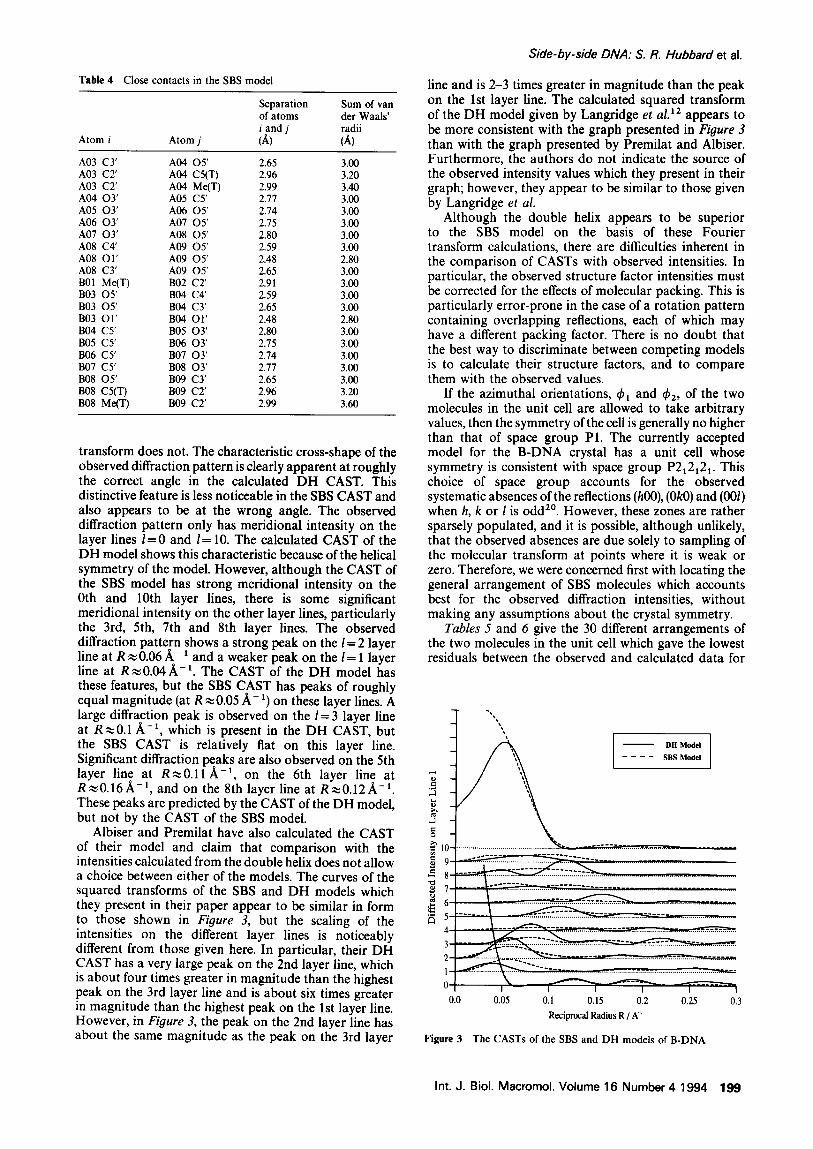
Table 4 Close contacts in the SBS model

Atom i Atom j

Separation of atoms i and j (A)

Sum of van der Waals' radii (A)

A03 C3' A04 05 ' 2.65 3.00 A03 C2' A04 C5(T) 2.96 3.20 A03 C2' A04 Me(T) 2.99 3.40 A04 O3' A05 C5' 2.77 3.00 A05 03 ' A06 05 ' 2.74 3.00 A06 03 ' A07 05 ' 2.75 3.00 A07 O3' A08 O5' 2.80 3.00 A08 C4' A09 05 ' 2.59 3.00 A08 O1' A09 O5' 2.48 2.80 A08 C3' A09 05 ' 2.65 3.00 B01 Me(T) B02 C2' 2.91 3.00 B03 05 ' B04 C4' 2.59 3.00 B03 05 ' B04 C3' 2.65 3.00 B03 O1' B04 O1' 2.48 2.80 B04 C5' B05 03 ' 2.80 3.00 B05 C5' B06 03 ' 2.75 3.00 B06 C5' B07 03 ' 2.74 3.00 B07 C5' B08 03 ' 2.77 3.00 B08 05 ' B09 C3' 2.65 3.00 B08 C5(T) B09 C2' 2.96 3.20 B08 Me(T) B09 C2' 2.99 3.60

transform does not. The characteristic cross-shape of the observed diffraction pattern is clearly apparent at roughly the correct angle in the calculated DH CAST. This distinctive feature is less noticeable in the SBS CAST and also appears to be at the wrong angle. The observed diffraction pattern only has meridional intensity on the layer l ines /=0 and l= 10. The calculated CAST of the DH model shows this characteristic because of the helical symmetry of the model. However, although the CAST of the SBS model has strong meridional intensity on the 0th and 10th layer lines, there is some significant meridional intensity on the other layer lines, particularly the 3rd, 5th, 7th and 8th layer lines. The observed diffraction pattern shows a strong peak on the l = 2 layer line at R ~ 0.06 A- 1 and a weaker peak on the l = 1 layer line at R ~0.04 A,-1. The CAST of the DH model has these features, but the SBS CAST has peaks of roughly equal magnitude (at R ~0.05 A-1) on these layer lines. A large diffraction peak is observed on the l= 3 layer line at R,,~0.1 A -1, which is present in the DH CAST, but the SBS CAST is relatively fiat on this layer line. Significant diffraction peaks are also observed on the 5th layer line at R~0.11/~ -1, on the 6th layer line at R~0.16A -1, and on the 8th layer line at R~0.12/~ -1. These peaks are predicted by the CAST of the DH model, but not by the CAST of the SBS model.

Albiser and Premilat have also calculated the CAST of their model and claim that comparison with the intensities calculated from the double helix does not allow a choice between either of the models. The curves of the squared transforms of the SBS and DH models which they present in their paper appear to be similar in form to those shown in Figure 3, but the scaling of the intensities on the different layer lines is noticeably different from those given here. In particular, their DH CAST has a very large peak on the 2nd layer line, which is about four times greater in magnitude than the highest peak on the 3rd layer line and is about six times greater in magnitude than the highest peak on the 1st layer line. However, in Figure 3, the peak on the 2nd layer line has about the same magnitude as the peak on the 3rd layer

Side-by-side DNA." S. R. Hubbard et al.

line and is 2-3 times greater in magnitude than the peak on the 1st layer line. The calculated squared transform of the DH model given by Langridge et al. lz appears to be more consistent with the graph presented in Figure 3 than with the graph presented by Premilat and Albiser. Furthermore, the authors do not indicate the source of the observed intensity values which they present in their graph; however, they appear to be similar to those given by Langridge et al.

Although the double helix appears to be superior to the SBS model on the basis of these Fourier transform calculations, there are difficulties inherent in the comparison of CASTs with observed intensities. In particular, the observed structure factor intensities must be corrected for the effects of molecular packing. This is particularly error-prone in the case of a rotation pattern containing overlapping reflections, each of which may have a different packing factor. There is no doubt that the best way to discriminate between competing models is to calculate their structure factors, and to compare them with the observed values.

If the azimuthal orientations, 41 and 42, of the two molecules in the unit cell are allowed to take arbitrary values, then the symmetry of the cell is generally no higher than that of space group P1. The currently accepted model for the B-DNA crystal has a unit cell whose symmetry is consistent with space group P212121. This choice of space group accounts for the observed systematic absences of the reflections (h00), (0k0) and (001) when h, k or I is odd 2°. However, these zones are rather sparsely populated, and it is possible, although unlikely, that the observed absences are due solely to sampling of the molecular transform at points where it is weak or zero. Therefore, we were concerned first with locating the general arrangement of SBS molecules which accounts best for the observed diffraction intensities, without making any assumptions about the crystal symmetry.

Tables 5 and 6 give the 30 different arrangements of the two molecules in the unit cell which gave the lowest residuals between the observed and calculated data for

, d

• "~ lO - - "" -" - -----. ::.'...-.... =.~.~ - .... '

2 ~ ~ - = w . : . ' ~ " 2 ' ' ' ~ : - = ~ : ~ . . . . . . . . . . ?" . . . . . . . . . . . . • . . . . . . . . . . . . . . . . . . . . . . . . . . . . . . . . . . . . . . . . . . . . . . . - . . . .

0[ -- I - - l I I I I

0.0 0.05 0.1 0. ! 5 0.2 0.25 0.3

Reciprocal Radius R / A t

Figure 3 The CASTs of the SBS and DH models of B-DNA



Table $ The 30 arrangements of the molecules in a crystalline SBS model which had the lowest values of the crystallographic residual R. The corresponding values of the penalty function P are given for each of these arrangements

q~l ~b2 Az R(~bl,~b2,Az ) P(~bl,tb2,Az ) (degrees) (degrees) (A) (%) (A- 2)

60.00 50.00 23.00 43.42 1222 30.00 30.00 23.00 43.68 1102 50.00 50.00 23.00 44.06 1594 60.00 60.00 23.00 44.12 1332 50.00 60.00 23.00 44.15 1328 50.00 80.00 6.00 44.24 2080 60.00 90.00 13.00 44.32 885

140.00 70.00 4.00 44.37 311 50.00 80.00 7.00 44.43 1943 50.00 60.00 11.00 44.43 1264 50.00 50.00 11.00 44.49 1546 60.00 270.00 23.00 44.49 800 60.00 50.00 23.00 44.51 1222 80.00 50.00 7.00 44.54 1086 30.00 30.00 23.00 44.57 1102 50.00 80.00 26.00 44.61 1329 60.00 60.00 11.00 44.62 1281 30.00 130.00 33.00 44.62 1025 50.00 300.00 33.00 44.63 556

130.00 60.00 4.00 44.69 548 90.00 240.00 23.00 44.71 1992

300.00 30.00 4.00 44.72 1329 60.00 90.00 14.00 44.72 650 60.00 270.00 23.00 44.72 800 20.00 230.00 23.00 44.73 1517 60.00 60.00 23.00 44.73 1332 90.00 80.00 23.00 44.74 875 60.00 70.00 23.00 44.78 1316 30.00 140.00 33.00 44.78 1091 80.00 50.00 6.00 44.80 944

Table 6 The 30 arrangements of the molecules in a crystalline DH model which had the lowest values of the crystallographic residual R. The corresponding values of the penalty function P are given for each of these arrangements

~bl q~2 Az R(~bl,q~2,Az) P(~bl,~2,Az) (degrees) (degrees) (,~) (%) (A -2)

20.00 20.00 23.00 34.33 109 90.00 90.00 23.00 34.52 113 50.00 90.00 14.00 34.71 66 20.00 270.00 13.00 34.85 59

160.00 200.00 14.00 34.89 70 50.00 50.00 23.00 34.90 198 90.00 230.00 24.00 34.91 295 90.00 20.00 4.00 34.92 58

130.00 20.00 13.00 34.94 108 20.00 310.00 4.00 34.95 127 90.00 200.00 33.00 35.02 128 20.00 130.00 33.00 35.07 303 20.00 200.00 6.00 35.08 82 90.00 230.00 3.00 35.16 66 50.00 270.00 31.00 35.22 65 60.00 200.00 24.00 35.23 335 90.00 270.00 6.00 35.26 110 20.00 160.00 24.00 35.30 198 20.00 60.00 14.00 35.31 152 90.00 50.00 7.00 35.32 296 20.00 90.00 30.00 35.36 110

160.00 20.00 31.00 35.37 69 20.00 160.00 3.00 35.38 71 60.00 90.00 14.00 35.39 368

130.00 200.00 30.00 35.51 107 60.00 20.00 7.00 35.58 331

130.00 200.00 17.00 35.60 265 90.00 50.00 20.00 35.61 66 50.00 230.00 6.00 35.65 149 20.00 50.00 14.00 35.69 276

the SBS and D H B - D N A models, respectively. The corresponding value of the penalty function P(~t,~2,Az) is also given for each of these arrangements. It is clear that, considering all the possible molecular arrangements, the R factor for the D H model assumes significantly lower values than the R factor for the SBS model. The lowest residuals for the D H model are approximately 10 percentage points less than the lowest residuals for the SBS model. We have found several hundred arrangements of D H D N A within the unit cell whose R factors are lower than 43,42%, which is the best value achieved by any arrangement of SBS molecules. Also, the arrangements giving the lowest R values for the D H model tend to have small values of the penalty function P, which indicates that there are few close intermolecular contacts in these arrangements. However, for the SBS model, almost all the arrangements giving the lowest R values have large values of P, suggesting that there is considerable steric hindrance between the molecules. These close contacts usually occur between O 1 P and O 2 P a toms in the phosphate groups of adjacent strands, but the P, 0 3 ' and CY atoms are also involved in some cases. Clearly, given a general arrangement of the molecules in the crystalline form of B-DNA, the SBS model is significantly worse then the D H model in account ing for the observed X-ray diffraction pat tern from these fibres, and its packing into the unit cell is also much less satisfactory.

The procedure adopted here is the s tandard method for testing proposed models against fibre diffraction data. However, it might be argued that it is biased, since the summat ion in the residual calculation is taken only over those Bragg reflections whose observed intensities are greater than the background. Any reflection with a lower intensity is deemed to have a zero amplitude, and it is omitted from the summation. If a proposed model predicted that such a reflection should have a significant intensity, this would go undetected. To overcome this deficiency, we have also tested a slightly modified procedure. The list of observed Bragg reflections was expanded to include all reflections which fell within the 3 A sphere. The amplitudes of the reflections which appeared in the Arnot t and Hukins set were unchanged, and any new reflections were assigned a zero amplitude. When residuals were calculated with this new dataset (results not shown), we found that 10-15 percentage points were added to the values obtained with the unmodified Arnot t and Hukins data for both the D H and SBS models. Similar results (not shown) were obtained when the new reflections were assigned an amplitude of 200, which is approximately half the threshold. Thus, a l though this modified procedure significantly worsens the residuals of the D H and SBS models, it does not affect our earlier conclusion that the D H model is superior to the SBS model.

We then considered molecular orientations which are consistent with the symmetry of the space group P21212 r This space group requires that the D N A molecule should contain at least one diad axis perpendicular to the molecular axis in each axial repeat unit (as both the D H and SBS models do), and that the diad axes of the two molecules in the unit cell should be parallel to each other and to either the a-axis (corresponding to ~b~ = (~2 = 0 ° ) or the b-axis (corresponding to q~x = ~b2 =90°). There is no limitation on the relative axial displacement, Az, of the two molecules, but extra absences, not required by


Side-by-side DNA." S. R. Hubbard et al.

Table 7 Values of the crystallographic residual R calculated for the crystalline DH and SBS models, in the molecular arrangements with q~l = ~2 = 90°, at different values of Az. The corresponding values of the penalty function P are also given for each of these arrangements. If the space group of the crystalline form is assumed to be P212t2~, then the allowed arrangements are those such that ~ =~b 2 =00,90 °

DH DNA SBS DNA

Az R(90°,90°,Az) P(90°,90°,Az) Az R(90°,90°,Az) P(90°,90°,Az) (A) (%) (A-2) (A) (%) (A-2)

0.0 58.14 0 0.0 67.29 792 1.0 49.27 270 1.0 57.28 1017 2.0 47.82 1023 2.0 54.52 3615 3.0 44.66 2465 3.0 51.74 2147 4.0 42.85 4737 4.0 51.93 2098 5.0 48.63 3161 5.0 57.64 1522 6.0 46.73 2317 6.0 55.31 1449 7.0 46.01 1233 7.0 56.19 1413 8.0 46.77 706 8.0 57.42 1792 9.0 41.96 145 9.0 51.87 1576

10.0 37.07 119 10.0 47.74 1453 11.0 36.06 107 11.0 46.82 2602 12.0 40.61 0 12.0 53.07 657 13.0 42.10 376 13.0 52.96 513 14.0 43.93 1239 14.0 53.69 599 15.0 46.93 2686 15.0 54.99 862 16.0 49.56 4192 16.0 54.47 1037 17.0 57.59 5489 17.0 62.75 1200 18.0 48.05 3571 18.0 54.19 981 19.0 45.34 2093 19.0 54.61 821 20.0 44.33 876 20.0 53.93 601 21.0 41.72 244 21.0 53.02 546 22.0 39.80 0 22.0 51.79 752 23.0 34.51 113 23.0 45.53 3439

24.0 37.44 116 24.0 47.87 1468 25.0 45.69 341 25.0 56.07 1743 26.0 44.80 907 26.0 55.67 1550 27.0 47.65 1676 27.0 56.89 1396 28.0 48.55 2779 28.0 57.17 1533 29.0 46.79 3404 29.0 56.49 1522 30.0 43.65 4116 30.0 52.27 2267 31.0 44.35 1818 31.0 51.17 2542 32.0 49.52 820 32.0 56.06 1959 33.0 50.37 122 33.0 58.75 781

this space group, are observed to occur in the diffract ion pa t t e rn f rom crysta l l ine B - D N A fibres when h + k is odd and I = 3m, where m is any integer. If these absences were systematic , they would imply that , for each molecule at (x, y, z), an ident ical one would exist a t ( x + 1/2, y + 1/2, z + 1/3). Hence, they require tha t Az = c/3. If one molecule were at the or igin with az imutha l o r ien ta t ion q~l, then the second molecule would be at (1/2, 1/2, 1/3), with az imutha l o r ien ta t ion ~b2=~bl=~ . In this case, the s t ructure fac tor of the Bragg reflection, F(hkl), is of the form:

F(hkl)=~.,, G,,t(R)exp{in(~+;-q~)}

x[l+expf i2 (h+k-+Li I( \2 2 3 / ; I (8)

This express ion clearly predic ts the absence of reflections

for which h+k is odd and l=3m. However , these reflections are only general ly no t sys temat ica l ly absent , and the list given by Arno t t and Huk ins conta ins eight reflections, namely (4,1,3), (3,2,3), (0,5,3), (4,1,6), (8,1,6), (7,2,6), (1,0,9) and (4,1,9), whose indices satisfy the above rule, and yet which have very significant intensities. The impl ica t ion of this is tha t the a r r angemen t of the molecules in the unit cell is subject only to the weaker cons t ra in t tha t Az ~ c/3.

Mos t of the a r r angemen t s of bo th D H and SBS D N A which have the lowest res iduals a p p e a r to occur when Az = 23.0 A (Tables 5 and 6). However , the a r r angemen t (q~l,~b2,Az) is equivalent to tha t with (~bl,~b2,c-Az). Hence, the a r r angemen t (~bl,~b2,23.0) is equivalent to (~bl,~b2,10.7). The value of 10.7 ~ is r easonab ly close to the accepted value of Az ~ c/3.

Tables 7 and 8 show the values of the R factor ca lcula ted for the crysta l l ine forms of bo th the D H and SBS mode l s of B - D N A at different values of Az, where



Table 8 Values of the crystallographic residual R calculated for the crystalline DH and SBS models, in the molecular arrangements with ~1 =~b2 =0°, at different values of Az. The corresponding values of the penalty function P are also given for each of these arrangements, which form the other set of possible arrangements consistent with P212121 being the space group of the crystalline form

DH DNA SBS DNA

Az R(O °,0 °,Az) P(0 °,0°,Az) Az R(0 °,0°,Az) P(0°,0°,Az) (A) (%) (A-2) (A) (%) (A-5)

0.0 70.44 6186 0.0 69.60 4013 1.0 61.96 3882 1.0 60.03 4254 2.0 57.64 2405 2.0 57.68 3787 3.0 50.05 1622 3.0 53.40 3983 4.0 50.60 933 4.0 52.93 3846 5.0 56.70 737 5.0 58.14 3575 6.0 53.74 922 6.0 57.24 3615 7.0 53.12 8537 7.0 56.91 4599 8.0 54.96 1556 8.0 56.50 3899 9.0 51.04 831 9.0 51.69 1457

10.0 45.32 602 10.0 49.11 1225 11.0 44.05 1094 i1.0 49.09 1142 12.0 50.85 1894 12.0 53.05 1049 13.0 52.73 3990 13.0 54.07 1101 14.0 52.64 3798 14.0 56.46 717 15.0 55.97 1996 15.0 59.24 370 16.0 56.30 1143 16.0 60.01 50 17.0 63.84 755 17.0 67.52 19 18.0 55.48 1325 18.0 59.34 130 19.0 55.04 2262 19.0 58.46 468 20.0 53.39 5190 20.0 55.80 808 21.0 52.13 3130 21.0 53.57 1057 22.0 49.43 1485 22.0 52.54 1054 23.0 42.50 583 23.0 48.01 1137 24.0 45.50 749 24.0 48.95 1216 25.0 54.22 967 25.0 55.05 1664 26.0 53.56 2110 26.0 55.25 3126 27.0 54.18 2902 27.0 57.80 51179 28.0 55.84 831 28.0 58.76 3636 29.0 54.59 662 29.0 56.55 3586 30.0 50.56 1006 30.0 52.66 3853 31.0 50.81 1658 31.0 53.98 3684 32.0 59.90 2641 32.0 59.30 3943 33.0 64.05 4715 33.0 61.73 4088

$ 1 = $ 2 = 9 0 ° or 0 °, respectively. The corresponding values of the steric hindrance penalty function are also given for these arrangements. The DH molecular arrangements in which t~l =~b2=90 ° have their lowest R value of 34.51% at Az=23 .0A or 10.7A. This arrangement also corresponds roughly to a minimum in the penalty function P, indicating that there is no steric hindrance between the two molecules. In the case of the SBS model, the values of the residual are approximately 10 percentage points higher than for the DH model. The lowest value of the residual in this arrangement, R=45.53%, also occurs at Az=23.0A. However, the penalty function P has a very large value, showing that there are many close intermolecular contacts. In the second possible arrangement, with t# t= t#2=0 °, the residuals for the DH model are significantly higher than in the first arrangement, with the lowest value being R = 42.50%, which again occurs at Az = 23.0 A. The value of the penalty function in this arrangement, P = 583 A- 2, indicates that there are a number of close intermolecular contacts. The SBS model has markedly higher residuals than the DH model in this second arrangement, with the lowest value of the residual being R--48.01%, at Az = 23.0 A; the value of the penalty function is 1137 A - 2 in this case.

Once we had confirmed that the best axial displacement of both models was approximately c/3, we attempted to define it as accurately as possible. Residuals were

calculated for values of Az between 10.5 A and 11.5 A in steps of 0.1A with ~bl=~b2=90 °. In each case, three different sets of observed structure factors were used in calculation of the residual. Dataset 1 consisted of the original observed structure factors of Arnott and Hukins 2°. Dataset 2 included the extra absences discussed above, assigning a zero amplitude to each. Dataset 3 was the same except that the extra absences were assigned a value of 200. The results of this analysis are shown in Table 9. When dataset 1 was used, the lowest values of the residual occurred at Az = 10.7 A for both the DH and SBS models. Inclusion of the extra absences did not substantially modify this conclusion: the optimum value of Az changed to 11.2 A when the absences were included with zero amplitude and to 11.0 A when they were included with an amplitude of 200. Therefore, we conclude that the optimum arrangements of the DH and SBS models consistent with space group P212~21 occur when ~b t =~b2 =90 ° and Az= 10.7 A.

The observed and calculated structure factors for the optimum arrangements of both the DH and SBS models are given in Table 10. The residuals between the calculated and observed structure factor amplitudes with these arrangements of the two models are R=45.53% for the SBS model and R=34 .51% for the DH model. The corresponding values of the penalty function P are 3439A -2 for the SBS model and l13A -2 for the DH model.


Table 9 Residuals and penalty functions of the DH and SBS models when Az ~ c/3 and q~l = ~b2 = 90 °. See text for explanation of the datasets

Dataset 1 Dataset 2 Dataset 3 R(90°,90°,Az) R(90°,90°,Az) R(90°,90°,Az) P

(%) (%) (%) (/~-2) Az (./~) DH SBS DH SBS DH SBS DH SBS

10.5 34.96 45.90 44.87 56.74 41.35 52.32 117 2165 10.6 34.52 45.59 43.40 55.44 39.99 51.14 115 2740 10.7 34.51 45.51 42.31 54.17 39.12 50.03 113 3439 10.8 34.99 45.58 41.59 52.98 38.68 49.08 111 3847 10.9 35.52 46.14 40.93 52.14 38.33 48.62 109 3355 11.0 36.06 46.80 40.22 51.44 38.07 48.46 107 2602 11.1 36.63 47.46 39.50 50.70 38.30 48.85 104 1985 11.2 37.19 48.19 38.73 49.99 39.63 50.45 0 1500 11.3 37.75 48.91 39.72 51.16 39.77 50.70 0 1188 11.4 38.23 49.59 41.53 53.18 39.83 50.80 0 1057 11.5 38.81 50.26 43.28 55.12 40.91 51,86 0 942

Discussion

The testing of a proposed model for fibrous DNA falls into two stages. In the first stage, the internal stereochemistry must be checked against standard bonded and non-bonded distances, and then the Fourier transform of the molecule must be calculated to see that it conforms, at least in general, with the observed distribution of intensities in the diffraction pattern. Both these procedures essentially treat the molecule as an isolated object. Tests of this type have been used exclusively in assessing the acceptability of previous SBS models. Most SBS models have had reasonable stereochemistry; none of them could have been rejected on the basis of stereochemistry alone, since small adjustments to the coordinates of a few atoms may alleviate any incorrect covalent bond lengths or close non-bonded contacts. The more controversial part of the first stage is the comparison of observed and calculated diffraction intensity distributions. Those who have proposed SBS models have made the point that the fibre diffraction data on which the double helix is based are of such poor quality that it is impossible to use them to discriminate between DH and SBS models. However, they have all used diffraction data from disordered or semi-crystalline fibres. The degree to which a calculated CAST agrees with such data is to some extent subjective, although it must be emphasized that, in our view, no SBS model has satisfactorily accounted for even this low- quality data. The latest model 1° does not appear to be significantly more successful than its predecessors in this regard.

The second stage of testing can only be undertaken when crystalline diffraction data are available. Once the dimensions of the unit cell and the number of molecules contained within it are known, the packing can be examined. It is clear that the Premilat and Albiser model cannot be packed into the observed B-DNA cell, since significant intermolecular short contacts are present for nearly all relative displacements and orientations of the two molecules, although it is possible that a least-squares refinement of the model would reduce the number and severity of these contacts. The failure of the SBS model to predict the observed structure factor intensities is a more serious deficiency. Its R factor is worse than that of the DH model by 9 percentage points (43.42% for SBS and 34.33% for DH) when general arrangements of the molecules are allowed, and by 11 percentage points


(45.53% for SBS and 34.52% for DH) when the symmetry of the cell is constrained to that of space group P212121. On the basis of these figures, the model with the higher R factors could be decisively rejected even if, for example, both models were double helices having a mononucleotide asymmetric unit. However, the SBS molecule has 10 nucleotides in the asymmetric unit and therefore has 10 times more degrees of freedom than the DH model. We have not used standard statistical tests to evaluate the confidence that we may have in these models, but there is no doubt that the SBS model could be rejected with greater than 99% confidence.

Several points can be made about the agreement between the observed and calculated structure factors which may be of significance in the design of any future models for DNA. For the purposes of this discussion, we have arbitrarily divided the Bragg reflections into weak (Fo < 2000), medium (2000 ~< Fo ~< 5000) and strong (Fo>5000) spots. There are 73, 61 and 17 reflections, respectively, in these categories.

The SBS model does not account adequately for the general distribution of intensities in the B-DNA diffraction pattern. In the case of the weak reflections, the SBS model over-estimates (+ ) the amplitudes of 54 spots and under-estimates ( - ) the amplitudes of 19 spots. For the medium reflections, the figures are + 18 and - 4 3 , and for the strong reflections they are + 0 and - 17. The results for the DH model are + 39 and - 3 4 in the case of weak spots, +30 and - 3 1 for medium spots, and + 4 and - 1 3 for strong spots. It is clear that the amplitudes calculated from the SBS model are significantly skewed, with a tendency to over-estimate the weak reflections and to under-estimate the medium and strong reflections. It is of particular note that all the strong reflections are under-estimated. In contrast to this, the amplitudes calculated from the DH model are more evenly distributed about the observed values.

Before discussing the level of agreement between the observed and calculated amplitudes of specific reflections, it is useful to consider the possible sources of error in the measurement of intensities and the calculation of transforms. The major contribution to errors in the observed intensities arises from the difficulty in determining the background scattering in a fibre diffraction pattern. The result of this baseline error is that weak intensities are measured to an accuracy of about +5 0 % of F o, and the error in strong reflections is probably about 10-15%. Errors in the calculated amplitudes may arise from the approximation made in accounting for the scattering from water and from neglecting any contribution from ions in the fibre. Water molecules and ions in ordered positions in the unit cell may make significant contributions to individual reflections. However, this effect should be small, especially since lithium was the counter-ion in the fibres from which the Arnott and Hukins data were recorded. A more significant error may arise, in the case of the DH model, from the assumption that the molecule is a perfectly regular helix. This is unlikely to be true for a DNA molecule with a random base sequence, since oligonucleotide crystals show that small-scale polymorphism is present which is dependent on the local base sequence (e.g. ref. 23). Therefore, in a DNA polymer, there are likely to be sequence-dependent perturbations of the helical structure which will not be taken into account when calculating the structure factors.


PO

2 T

ab

le

10

Ob

serv

ed

an

d c

alcu

late

d s

tru

ctu

re f

acto

r a

mp

litu

de

s fo

r th

e S

BS

an

d D

H

B-D

NA

mo

de

ls

d(hk

l) lE

e[

IF01

d(

hkl)

IF

¢l

IFcl

d(

hkl)

IF

cl

IFJ

d(hk

l)

IF¢l

IF

¢I

d(hk

l)

IF01

IF

J d(

hkl)

IF

0[

IFJ

hkl

(A)

[Fo[

SB

S D

H

hkl

(A)

IFol

SB

S D

H

hkl

(A)

IFol

SB

S D

H

hkl

(A)

lEo[

SB

S D

H

hkl

(A)

IF.I

SB

S D

H

hkl

(A)

IF.l

SBS

DH

2 0

0 15

.40

1930

29

6 67

3

0 1

9.82

1

06

1

1902

82

7 3

2 2

6.92

53

1 1

69

8

1210

5

3 3

4.38

32

17

1917

26

19

3 3

5 4.

50

1287

48

3 36

0 1

2 7

4.38

i

O 3 o_.

< o_.

e-" 3 ¢1)

Z

e- 3 O" o 4~

tO

¢,D

3 1

0 9.

34

2467

21

81

2506

3

1 1

9.00

96

5 18

91

804

1 3

2 6.

69

6 2

3 4,

31

3325

13

99

4545

5

1 5

4.46

12

87

1047

36

7 3

0 7

4.36

2 2

0 9.

08

3754

31

47

3192

2

2 1

8.77

42

9 11

27

936

4 1

2 6.

69

1394

22

50

663

0 5

3 4.

18

3641

28

2 58

9 1

4 5

4.28

55

77

2158

33

92

3 1

7 4.

28

4 0

0 7.

70

2896

2

18

1

2684

0

3 1

7.32

2

3 2

6.26

15

01

2758

71

1 1

5 3

4.14

31

10

4101

40

96

5 2

5 4.

22

2 2

7 4.

25

1 3

0 7.

29

1394

1

97

8

3090

3

2 1

7.40

91

0 16

10

1157

5

0 2

5.79

2

5 3

4.03

4

3 5

4.20

56

84

3724

43

55

1 3

7 4.

02

4 2

0 6.

35

2145

1

71

1

14

85

1

3 1

7,12

3

3 2

5.70

7

1 3

4.03

39

68

4371

40

37

6 0

5 4.

08

4 1

7 4.

02

3 3

0 6.

06

858

2032

58

6 4

1 1

7.12

75

1 93

1 14

05

5 1

2 5.

60

2124

27

73

2135

3

5 3

3.87

17

16

4463

27

05

6 1

5 4.

02

1214

19

50

1353

2

3 7

3.92

5 1

0 5.

94

536

1233

12

1 2

3 l

6.61

96

5 1

27

1

1414

1

4 2

5.26

28

96

2453

32

65

0 6

3 3.

56

3217

99

1 18

14

0 5

5 3.

74

5 1

7 3.

74

0 4

0 5.

63

858

1226

67

1 4

2 1

6.24

64

3 13

20

1685

5

2 2

5.15

2

6 3

3.47

1

5 5

3.72

2

0 8

4.06

2 4

0 5.

28

5791

46

17

6026

5

0 1

6.06

85

8 1

10

8

2110

4

3 2

5.12

33

25

2500

44

78

8 2

3 3.

46

7 0

5 3.

68

1896

32

62

498

2 1

8 4.

00

6 0

0 5.

13

6649

29

13

4073

3

3 1

5.96

64

3 99

5 12

69

6 1

2 4.

80

5 5

3 3,

46

3646

30

48

5645

6

3 5

3.59

1

2 8

3.91

5 3

0 4.

76

2896

26

25

3224

1

4 1

5.46

1

82

3

2634

21

05

3 4

2 4.

73

3217

2

10

1

3771

0

7 3

3,09

5

4 5

3.54

24

67

2472

27

57

3 0

8 3.

90

4 4

0 4.

54

2038

1

00

8

1288

5

2 1

5.33

0

5 2

4.35

5

6 3

3.08

1

1 6

5.37

75

1 12

29

1304

3

1 8

3.84

7 1

0 4.

32

751

2176

51

3 4

3 1

5.3

1

2788

30

13

234

1 5

2 4.

30

1 7

3 3.

07

2 0

6 5.

28

1501

23

7 11

61

2 2

8 3.

82

3 5

0 4.

12

2467

17

44

2558

2

4 1

5.22

16

09

2115

21

81

7 0

2 4.

26

1896

17

29

2542

8

4 3

3.06

20

48

3741

34

37

0 2

6 5,

03

1930

15

43

2412

3

2 8

3.68

8 0

0 3.

85

7614

19

14

3985

6

1 1

4.95

2

5 2

4.18

1

1 4

7.64

7 3

0 3.

80

3 4

1 4.

88

2038

18

16

3118

7

1 2

4.18

16

09

4067

34

51

2 1

4 7.

02

6 4

0 3.

79

4075

34

04

4094

5

4 1

4.12

1

50

1

2571

32

00

6 3

2 4.

11

1609

18

06

3280

1

2 4

6.59

0 6

0 3.

75

5899

1

64

9

2904

7

2 1

4,07

1

50

1

2894

24

56

5 4

2 4.

03

3 0

4 6.

51

2 6

0 3.

64

4 5

1 3.

86

3 5

2 4.

00

3 1

4 6.

26

8 2

0 3.

64

8 0

1 3.

83

2427

1

63

8

3269

7

2 2

3.98

45

04

2807

39

71

2 2

4 6.

18

5 5

0 3.

63

1093

9 26

92

6990

8

1 1

3.77

4

5 2

3.79

1

3 4

5.51

9 1

0 3.

38

6 4

1 3,

77

8 0

2 3.

75

2199

29

32

2035

4

1 4

5,51

4

6 0

3.37

31

10

11

67

19

50

7 3

1 3.

77

3754

36

70

4915

1

1 3

9.55

38

61

2467

48

19

5 2

4 4.

55

322

2146

19

1 2

2 6

4.78

16

09

3435

29

28

0 3

8 3.

67

858

1444

75

4 4

0 6

4.54

51

48

875

2769

1

3 8

3.65

751

3246

87

3 1

3 6

4.45

4

1 8

3,65

643

1459

62

4 4

1 6

4.45

36

46

2433

47

25

2 3

8 3.

57

4 2

6 4.

21

5362

28

37

6537

5

0 8

3,48

536

2707

15

44

5 1

6 4.

08

643

16

08

20

50

4 3

8 3.

32

5 3

6 3.

63

1501

15

09

1127

2

4 8

3.29

965

2175

26

73

1 5

6 3.

49

3217

19

88

2681

1

0 9

3.72

2

5 6

3,42

0

2 9

3.55

1517

27

07

2303

1394

33

00

1342

2359

25

22

1358

1609

20

96

749

858

1214

60

858

267

222

4612

26

22

329

7888

60

21

5343

4502

24

47

6201

4550

27

71

2719

5470

43

35

3243

18

23

23

48

3463

2896

18

49

1900

1930

16

99

1529

2359

89

4 77

6

2574

1

12

1

2515

1 7

0 3.

20

1 6

1 3.

70

2 0

3 9.

08

4826

73

6 45

08

4 3

4 4,

53

1930

23

74

1564

7

1 6

3.42

18

23

1857

29

74

3 1

9 3.

48

8 4

0 3.

18

1180

14

49

2218

2

6 1

3.62

0

2 3

7.95

43

97

3578

45

25

3 4

4 4.

26

2896

30

63

2371

3

5 6

3.32

2

2 9

3.46

28

96

6155

37

31

7 5

0 3.

15

5 5

1 3.

61

3 1

3 7.

18

2788

29

42

4140

7

4 4

3.21

28

96

2269

25

09

7 2

6 3.

31

1716

1

93

5

2679

1

3 9

3.33

9 3

0 3.

11

2359

1

71

8

2507

8

2 1

3.62

2

2 3

7.06

20

38

19

81

22

92

0 1

5 6,

46

643

389

56

7 3

6 3.

14

4 1

9 3,

33

2145

22

53

773

10 0

0

3.08

3

6 1

3.50

39

68

4955

39

31

4 0

3 6.

35

2 1

5 5.

95

643

2193

39

16

6 4

6 3.

14

1 1

10

3.3

1

3 7

0 3.

07

1 0

2 1

4.7

8

3432

27

24

2832

3

2 3

6.29

18

20

1424

19

79

1 2

5 5,

68

8 1

6 3.

14

2252

36

47

2485

2

0 10

3.

29

1756

9 16

512

1716

7

6 6

0 3.

03

2882

43

08

710

0 1

2 1

3.4

9

4933

39

68

4127

1

3 3

6.11

3

0 5

5,63

64

47

4686

75

09

2 6

6 3.

06

2 1

10

3.26

1 0

1 22

.74

26

81

10

56

2757

1

1 2

12

.35

28

96

2078

30

02

4 1

3 6.

11

965

3693

23

35

3 1

5 5.

47

965

779

1152

8

2 6

3.06

0

2 10

3.

23

8192

76

00

8454

0 1

1 18

.71

3861

2

10

1

2739

2

0 2

11

.37

34

32

1959

20

59

4 2

3 5

.53

10

72

4040

70

0 2

2 5

5.41

96

5 92

0 54

8 5

5 6

3.05

16

09

2426

20

26

1 2

10

3.21

1 1

1 15

.99

1072

36

24

2064

2

1 2

10

.15

46

12

2217

47

68

3 3

3 5.

33

2574

29

58

3434

3

2 5

5.04

1

0 7

4,76

85

8 10

80

289

3 0

10

3.20

78

12

4128

43

55

2 0

1 14

.01

536

401

1004

0

2 2

9.36

1

28

7

790

915

5 1

3 5.

25

2252

40

55

2852

0

3 5

5.01

58

40

5802

46

41

1 1

7 4.

65

1716

26

22

1487

1

3 10

3.

06

2 1

1 11

.89

322

5650

63

9 1

2 2

8.95

0

4 3

5.03

13

94

1117

60

4 1

3 5

4.95

2

1 7

4.50

16

09

1536

19

41

4 1

10

3.06

15

01

2332

10

95

0 2

1 10

.67

643

301

190

3 0

2 8.

77

2882

49

21

1859

2

4 3

4.78

18

23

1102

11

82

4 1

5 4.

95

5362

37

16

2433

1 2

1 10

.08

4 0

2 7.

00

6 0

3 4.

67

3003

25

20

1094

2

3 5

4.77

19

30

1389

15

21

• h,

k a

nd I

den

ote

the

Mil

ler

indi

ces

of e

ach

refl

ectio

n •

d(hk

l) is

the

spa

cing

of

the

crys

tal

plan

es h

kl a

nd

is

give

n by

:

[-h

2 k 2

12

] -~

,2

d(hk

l)=L-

a~ +

~+

~J

• tF

ol is

the

obs

erve

d st

ruct

ure

fact

or a

mpl

itud

e of

eac

h re

flec

tion

(ref

. 20

). T

he

refl

ectio

ns

in t

he l

ist

for

whi

ch n

o va

lue

of I

Fol i

s gi

ven

are

over

lapp

ing

refl

ectio

ns,

whi

ch o

ver

lap

wit

h th

e ne

xt r

efle

ctio

n in

the

lis

t fo

r w

hich

a v

alue

of

IFol

is

cite

d. T

his

valu

e of

IFo

l cor

resp

onds

to

the

squa

re r

oot

of t

he t

otal

int

ensi

ty o

f th

e o

ver

lap

pin

g r

efle

ctio

ns

• IF

cl S

BS

is t

he s

truc

ture

fac

tor

ampl

itud

e of

eac

h re

flec

tion,

ca

lcul

ated

for

the

SB

S m

odel

hav

ing

the

arr

ange

men

t: ~

b~ =

~b 2

=9

0.0

0 °

and

Az=

10.

7 A

. T

he

resi

dual

R b

etw

een

the

calc

ulat

ed a

nd

obs

erve

d st

ruct

ure

fact

or a

mpl

itud

es f

or t

his

arra

ng

emen

t of

the

SB

S m

odel

= 4

5.51

%

• N

Fcl

DH

is

the

stru

ctur

e fa

ctor

am

plit

ude

of e

ach

refl

ectio

n,

calc

ulat

ed f

or t

he D

H m

od

el h

avin

g th

e ar

rang

emen

t: ~

b~ =

~b 2

= 9

0.00

° an

d A

z =

10.

7 A

. T

he

resi

dual

R b

etw

een

the

calc

ulat

ed a

nd o

bser

ved

stru

ctur

e fa

ctor

am

plit

udes

for

thi

s ar

rang

emen

t of

the

DH

mod

el =

34.

51%

We have arbitrarily defined reflections for which F c is outside the range Fo++_½Fo as at variance with the observed amplitude given the possible sources of error discussed above. In the category of weak reflections, the SBS model predicts that 41 reflections satisfy this criterion, whereas 38 do so for the DH model. In view of the large errors of measurement associated with weak reflections, we do not believe that these apparently large numbers of deficiencies in the predicted amplitudes cast serious doubt on the acceptability of either of the models. However, in the case of the SBS model, three reflections, namely (2,1,1), (1,1,4) and (2,2,4), have predicted amplitudes which are very large, although only small amplitudes are observed. The DH model has one reflection, (2,1,5), which suffers from this problem.

The SBS and DH models also predict that 20 and 12 medium reflections, respectively, and 5 and 2 strong reflections, respectively, have calculated amplitudes which lie outside the range defined above. The presence of strong reflections in the diffraction pattern indicates that there is a high concentration of atoms in the corresponding crystalline planes, so the inability of any model to account for their observed amplitudes must be regarded as a particularly serious deficiency. It is noteworthy that the SBS model does not account adequately for nearly one-third of the strong reflections. It may be pertinent to observe that four of the five reflections are equatorial, namely the (6,0,0), (8,0,0), (0,6,0) and (5,5,0) spots. Indeed, there is only one strong equatorial reflection, (2,4,0), for which the SBS model accounts satisfactorily. In contrast, the DH model only fails to account for one equatorial reflection, (0,6,0). Since these reflections arise from the projection of the structure along the c-axis, they are sensitive to the rotational symmetry of the molecule. It is tempting to conclude that the failure of the SBS model and the success of the D H model in predicting equatorial amplitudes arise simply because the DNA molecule has the high rotational symmetry possessed by the DH model but not by the SBS model.

The other area of the diffraction pattern in which there is a concentration of strong reflections is the 10th layer line. Diffraction on this layer line is dominated by the stacking of the bases, although the positions of the phosphate groups can have a significant effect 17. Both models account reasonably well for these strong reflections. This is not unexpected since the base stacking is similar in both cases, with Watson-Crick base pairs approximately perpendicular to the helical axis.

C o n c l u s i o n

The work presented here underlines the point that


crystalline diffraction data should be used when testing proposed models since they provide an objective and quantitative measure of the acceptability of the models. It also illustrates the degree of confidence that we may have in the large number of double helical conformations that have been determined from crystalline fibrous diffraction data. The model described by Premilat and Albiser, although ultimately unsuccessful in displacing the double helix as the best model for B-DNA in fibres, has allowed us to set the standard against which any future model should be judged.

Acknowledgements We are grateful to the Science and Engineering Research Council for the provision of a Research Studentship to S.R.H.

References 1 Watson, J.D. and Crick, F.H.C. Nature 1953, 171, 737 2 Rodley, G.A., Scobie, R.S., Bates, R.H.T. and Lewitt, R.M. Proc.

Natl Acad. Sci. USA 1976, 73, 2959 3 Sasisekharan, V. and Pattabiraman, N. Curr. Sci. 1976, 45, 779 4 Sasisekharan, V. and Pattabiraman, N. Nature 1978, 275, 179 5 Bates, R.H.T., Lewitt, R.M, Rowe, C.H., Day, J.P. and Rodley, G.A.

J. Proc. R. Soc. N Z 1977, 7, 273 6 Bates, R.H.T., McKinnon, G.C., Millane, R.P. and Rodley, G.A.

Pramana 1980, 14, 233 7 Sasisekharan, V., Pattabiraman, N. and Gupta, G. Proc. Natl

Acad. Sci. USA 1978, 75, 4092 8 Albiser, G. and Premilat, S. Biochem. Biophys. Res. Commun.

1980, 95, 1231 9 Miilane, R.P. and Rodley, G.A. NucL Acids Res. 1981, 9, 1765

10 Premilat, S. and Albiser, G. Biochem. Biophys. Res. Commun. 1982, 104, 22

11 Langridge, R., Marvin, D.A., Seeds, W.E., Wilson, H.R., Hooper, C.W., Wilkins, M.H.F. and Hamilton, L.D.J. Mol. Biol. 1960, 2, 38

12 Langridge, R., Wilson, H.R., Hooper, C.W., Wilkins, M.H.F. and Hamilton, L.D.J. Mol. Biol. 1960, 2, 19

13 Fuller, W. and Mahendrasingam, A. in 'Topics in Nucleic Acid Structure', Part 3 (Ed S. Neidle), Macmillan Press, Basingstoke, 1987, p 101

14 Greenall, R.J., Pigram, W.J. and Fuller, W. Nature 1979, 282, 880 15 Arnott, S. Nature 1979, 278, 780 16 Arnott, S. Trends Biochem. Sci. 1980, 231 17 Greenall, R.J. PhD Thesis, University of Keele, 1982 18 GreenaU, R.J. in 'Topics in Nucleic Acid Structure', Part 3

(Ed S. Neidle), Macmillan Press, Basingstoke, 1987, p 133 19 Arnott, S. and Hukins, D.W.L Biochem. Biophys. Res. Commun.

1972, 47, 1504 20 Arnott, S. and Hukins, D.W.L J. Mol. Biol. 1973, 81, 93 21 Cochran, W., Crick, F.H.C. and Vand, V. Acta Crystallogr. 1952,

5, 581 22 Hubbard, S.R. DPhil Thesis, University of York, submitted 1994 23 Drew, H.R., Wing, R.M., Takano, T., Broka, C., Tanaka, S.,

Itakura, K. and Dickerson, R.E. Proc. Natl Acad. Sci. USA 1981, 78, 2179


Structure factor calculations for a side-by-side model of B-DNA

Documents

Transcript of Structure factor calculations for a side-by-side model of B-DNA