Amenity Value of Forests in Great Britain and

its Impact on the Internal Rate of Return from

Forestry

K. G. WILLIS and G. D. GARROD

Countryside Change Unit, Department of Agricultural Economics and Food Marketing,University of Newcastle upon Tyne, Newcastle upon Tyne, NE1 7RU, England

SUMMARY

The amenity value of trees was measured by observing how house prices variedaccording to differences in the type, composition, and age of forests and woodland inthe neighbourhood of each property, holding all other variables constant. Statisticallysignificant differences were detected. Broadleaved trees had a positive effect on houseprices, while mature Sitka spruce reduced housing values. The estimated amenityvalues were incorporated into discounted cash flow rotation models in order to assessthe joint value of the timber and amenity values of different rotations. The aggregatewood and amenity value which produced the highest internal rate of return and thelargest net present value was the one in which broadleaved oaks replaced Sitka spruce.

INTRODUCTION

Hedonic pricing is an increasingly popular method for valuing the attributesof housing and other goods. It is based on the observation that goods arevalued for their utility bearing attributes or characteristics. Hedonic pricingprovides a way of estimating how the value of a good would vary if certainchanges were to be made to its characteristics. In the case of housing, thehedonic price model can be used to estimate the change in house pricesassociated with alterations in the levels of various structural, locational andenvironmental characteristics.

The proximity of woodland to a property may influence house pricedepending on the age and composition of that woodland, and this effect canbe modelled using the hedonic price technique, and the values of any changesto the woodland, as reflected in house prices, can also be estimated.

Such monetary valuations of woodland and other forested areas areimportant for several reasons. First, since individual households may expressa demand for trees and woods as a housing attribute, knowledge of thisdemand is clearly of interest to those bodies involved in proposals for newdevelopment. Second, externalities created by forests are important to theForestry Commission in redesigning and restocking forest when felled and in

Forestry, Vol. 65, No. 3,1992

332 Forestry

modifying the rotation period or tree mix of forest blocks, to maximize thecombined value of timber and external amenity and other benefits. Third, theexternal benefits created by woods and forests are important factors in severaldecision-making processes including the determination of government policywith respect to setting the appropriate level of recreation and amenity subsidyto the Forestry Commission; the rate of expenditure on tree protection bylocal government; the design, planning and subsidy towards small woods inthe countryside; and the design, scale, distribution of, and subsidy to,urban forests.

A study by the National Audit Office in 1986 into the non-priced recreationbenefits of the Forestry Commission forest estate, suggested a figure forconsumer surplus of f 10 million per year, based on the cost of travelling tomake use of them. However, the accuracy of this estimate, based on a travel-cost study for one site in the late 1960s, indexed up to 1986, was the subject ofsome debate. The House of Commons Committee of Public Accounts (1987)recommended that a great deal more quantification should be carried out, tomeasure the performance of secondary Forestry Commission objectives suchas the provision of recreation facilities, because there was insufficientquantification of these benefits in a commensurate way with resource costsand timber returns.

In response to these recommendations, a series of travel-cost studies ofrecreation visitors was carried out, covering a wide variety of sites in 15 forestdistricts. A zonal travel-cost method (ZTCM) estimated an average consumersurplus of £2.00 per visitor over these sites in 1988 prices (Willis and Benson,1989; Willis, 1991). Consumer surplus varied between areas from £3.31 atLoch Awe, £2.72 at Aberfoyle, to £1.43 at New Forest and £1.34 at the SouthLakes area. Aggregating over the number of visitors to different types offorest, this analysis suggested that the non-priced recreational benefit of thewhole Forestry Commission estate was worth £53 million per annum.However, given the varying number of visitors to different areas and the sizeof forested area, consumer surplus per hectare from recreation varied fromless than £1 per ha at Loch Awe and £2 at Lome, to £425 at New Forest, and£449 per ha in Cheshire.

Forests produce benefits over and above recreation use benefits, and totalbenefits may be reflected in property values since, ceterisparibus, the price ofa house reflects willingness to pay (WTP) to live near an environmentalamenity such as a forest to gain access to it, and also the amenity (non-use orindirect use) value of the forest in so far as it creates a pleasant landscape.

This paper derives implicit prices for the effect of different types of foreston house value. These prices are subsequently used in discounted cash flowforest rotation models to investigate future expansion and replantingrotations which would maximize the joint value of timber and externalamenity benefits of woodland.

Amenity Value of Forests 333

THE DATA

Data from a large national building society of every mortgage approved bythe society in 1988 was used as the database in this study. This covered over100,000 properties distributed throughout the country. Each individualtransaction record included details of the selling price, the number of roomsand other structural characteristics of the house such as central heating,floorspace and garaging, as well as the personal characteristics of theoccupiers, such as income and family composition.

This data set meets the dual requirements of any study investigating theeffects of external factors, such as woodland, on house price. First, it containsa large amount of data detailing the structural characteristics of the propertiesinvolved, in order to explain those differences in price attributable tovariations in the physical characteristics of the houses, as opposed to thosewhich are the result of variation in external factors. Second, the area coveredby the data is sufficiently wide to ensure a representative spread of variationin the level of any external factors being investigated.

Since individual mortgaged properties were identified locationally by,among other indicators a grid reference, this permitted records to be matchedto those kept by the Forestry Commission (FC) detailing the location andcomposition of their holdings. Properties located in a grid square containingFC land were isolated and used as a database for a hedonic price study.

The FC database contains detailed information on the composition of treestocks for small units of FC land. This was aggregated into individual recordsfor all those 1 km Ordnance Survey grid squares in Great Britain containingpart of the FC estate. These records give details of the percentage of forestedarea covered by the six main age groups of each of the following three maincategories of planting: (1) all broadleaved trees (2) larch, Scots pine andCorsican pine (3) all other conifers; information is also present concerning thepercentage of forested land in various windthrow hazard classes; and on thetotal FC, and FC forested land, attributable to each 1 km square.

What the database fails to provide, are details of the size and compositionof any non-FC forested area in a particular 1 km square, or in those squareswhich do not encompass any FC land. This means that there is no reliable wayof estimating total tree cover by age and type over all 1 km grid squares inGreat Britain, and because of this no way of including the 'without forestry'case in the data set.

Because those squares incorporating part of the FC estate may wellencompass non-FC woodland, it would be inappropriate for estimates to bedriven by details of the distribution of total forest cover. Instead the variablesused in the model are the measures of the relative proportion of forested areacovered by each specified tree category. This, of course, assumes that thecomposition of private woodland in a particular 1 km square is similar to thatof the FC woodland in the same square, which may not always be the case.

In addition to data on the structural characteristics of a property, it was also

334 Forestry

necessary to know something about its neighbourhood, particularly the socio-economic composition of the population and the labour marketcharacteristics of the locality. The principal sources of this sort of informationare 1981 Census small area statistics and data from the Department ofEmployment's National Online Manpower Information System (NOMIS).The 1981 census small area statistics provide information at a local level onvariables such as population density, proportion of population over 60 yearsof age and the number of households with two or more cars (a proxy for localaffluence). NOMIS on the other hand can provide regularly updated statisticson the labour market including monthly or quarterly information onunemployment, details of existing vacancies and triennial breakdowns of thenumber of people employed in a range of industrial categories.

THE HEDONIC PRICE MODEL

The hedonic house price model is specified as:

Pi=f(FQ,QhShSEhRi) [1]

where:

Pi = the market price of property iFCi = a vector of the forest and woodland characteristics in the

neighbourhood of the ith propertyQt = the quarter of the year in which the /th property was purchased5, = a vector of the structural characteristics of the ith propertySEj = a vector of variables describing the socio-economic characteristics of

the local area containing the ith propertyRt = the region in which the /th property is located, to account for price

variations due to different housing market areas.

The model, which was derived using multiple regression techniques, isdescribed in more detail in Garrod and Willis (1991). Variables were dividedinto three categories: focus, free and other variables. Focus variables werethose of particular interest from a policy point of view, and in this caseconsisted of the woodland characteristics contained in vector FCt. Freevariables, were defined as those variables, such as structural characteristicsand time of sale, which were known to affect property values but which wereof no special interest to the study. There remained the other variables, thosewhich may or may not have affected the dependent variable in some way.These included local socio-economic characteristics and the region in whichthe property was located. Only a few neighbourhood characteristics (e.g.unemployment, percent of working population employed in agriculture) wereconsidered in this study due to difficulties with data collection. The lack offurther neighbourhood variables may not, however, have been too important.Several studies, including Butler (1982) and Follain etal. (1979), have foundevidence that the errors induced into individual coefficient estimates by the

Amenity Value of Forests 335

omission of neighbourhood variables are sufficiently small that such variablesmay be safely ignored for most purposes. So, given that at least someneighbourhood variables were included in this model the omission of anyfurther variables should not have unduly affected coefficient values.

The only focus variables considered for inclusion in the model were thoserepresenting the proportions of FC forested area covered by the followingthree tree categories: (1) all broadleaved trees; (2) larch, Scots pine andCorsican pine planted before 1920; (3) all other conifers planted before 1940excluding larch, Scots pine and Corsican pine. These three were chosen froma full set of focus variables, reflecting a complete range of forest categoriesand ages, after preliminary investigations had identified them as the only onesrepresentative of the relative density of forestry in a 1 km square which couldbe usefully constructed from current FC records and which did not displayany significant level of intercorrelation. Clearly, this set of focus variablesexcluded all conifers planted after 1940 and all larch, Scots pine and Corsicanpine planted after 1920 — groups which contain a large part of the FC'sholding. However, this was not an attempt to ignore the effects of commercialforestry on a roughly 50-year rotation, but a response to statistical problemsin analysing the data.

The free and other variables were selected on the basis of their inclusion inprevious studies (e.g. Cobb, 1984; Nicholson and Willis, 1991) and, mostimportantly, on the basis of their availability. All variables initiallyconsidered for inclusion in the model are documented in the Appendix.

The implicit price of an individual characteristic or amenity can be found bydifferentiating the hedonic price model (Equation 1) with respect to thatcharacteristic. If the functional form of the hedonic price function is non-linear this implies a variable price unit.

Economic theory fails to indicate any particular functional form as beingappropriate for the hedonic price function. However, Cropper etal. (1988)give a useful practical insight into which functional form to use. For cases suchas this one, where some important explanatory variables were known to bemissing, Cropper et al. state that simpler functional forms such as the linear,semi-log, double-log and Box-Cox linear perform best, with quadratic forms,including the quadratic Box-Cox, faring relatively badly. This poorperformance is attributed to the fact that for quadratic forms, each marginalprice is dependent on more coefficients than in other cases. Thus, omittedvariable bias affects more coefficients in the quadratic case than in others,implying that this form should be rejected when mis-specification is a knownfactor. Previous studies of a similar nature (e.g. Nicholson and Willis, 1991)have also shown that the use of the second order terms introduced additionalmulticollinearity problems, which reduced the significance of first order termswithout making any significant improvement to the fit. With respect to thequadratic Box-Cox functional form, Cassel and Mendelsohn (1985) point outthat if a large number of coefficients are estimated the accuracy of theestimation of single coefficients is reduced, which could lead to poorer

336 Forestry

estimations of marginal cost. This, coupled with the aforementioned advice ofCropper et al. (1988), led to a concentration on the linear Box-Coxtransformation which is the approach strongly favoured by Cropper et al.

AMENITY VALUE RESULTS

Table 1 documents the estimates of the hedonic price model using the abovespecification. Over 75 per cent of the variation in the dependent variable wasexplained, though only a small proportion of the explanatory power wascontributed by the focus variables. The remaining variation in the model mayhave been explained by omitted variables and measurement errors.

Focus and free variables were incorporated in the final model on the basisof significant coefficient values and a priori expected signs. Only two of thethree focus variables, BROAD and CON40, were included in the final model.In preliminary regression models the variable LARP20 was shown not to havea significant coefficient value and was therefore omitted from the final model(though a version of the model including this variable was estimated and willbe discussed later).

By using the coefficient values specified in Table 1 and holding all othervariables at their mean level, the implicit prices of the explanatory variableswere calculated. Thus, a unit increase of the proportion of FC forested area ina given 1 km square into broadleaved woodland was shown to raise theexpected selling price of a property by £42.81 when all other independentvariables were held at their mean values. A similar increase in the proportionof mature conifers (excluding larch, Scots pine and Corsican pine) reducedthe expected selling price of a house by f 141. It must be borne in mind whenconsidering this figure, that the high levels of statistical correlation betweenthe variable CON40 and the omitted variables representing the youngerconifer groups, may have meant that some of the effects of those youngerconifers on house prices were reflected in the implicit prices of CON40.

The effects of omitting focus variables from the model due tointercorrelation problems are hard to measure, however, one focus variablewas omitted from the final model because it was found to be statisticallyinsignificant at the 10 per cent significance level and the effect of its exclusionon the implicit prices of the other focus variables can be investigated. In orderto do this, and at the same time to examine the potential effect of maturelarch, Scots pine and Corsican pine on house prices, the variable LARP20was included in an extended model. While the coefficient of LARP20 was notstatistically significant its sign was positive, indicating that increasing theproportion of mature larch, Scots pine and Corsican pine may in fact raiseproperty values (by f 20.33 per unit increase in forested area).

The inclusion of the LARP20 variable in the model reduced the implicitprice of broadleaved woodland slightly to £42.33 and raised the implicitprice of the CON40 conifers to —£143.03. These changes implied that thecoefficient values of the focus variables, and hence the estimates of implicit

Amenity Value of Forests 337

TABLE 1: Hedonic price model: coefficient estimates

Coefficient r-ratio

Intercept 12.2942

Focus variablesBROAD*CON40*

Free variablesBATHSDETACHBPB*TERRGARFULLCHPARTCHFLOOR*SQTRLQTRBMKT1BMKT2BMKT8BMKTRM

Other variablesDIST4DIST6DIST7DIST10DIST11DIST12RETD*PDEN*AG*NOCAR*UNEM*

0.0126-0.0938

0.55290.5920

-0.4087-0.3755

0.33920.23180.15930.0259

-0.11520.2091

-1.9579-1.4982-0.6702-0.2972

0.3994-0.4417-0.3853-0.2824

0.5702-0.5292

0.18690.07110.04%

-0.0750-0.1287

35.64

2.73-2.95

6.079.92

-4.87-7.37

6.774.221.783.02

-2.314.17

-7.48-18.64-7.91-3.89

2.36-5.01-3.78-2.37

5.79-4.49

4.803.581.82

-1.81-3.89

•Transformed using Box-Cox transformation

338 Forestry

price, were somewhat susceptible to variable specification. However, thefocus variables did not show any significant degree of intercorrelation withany other variables in the model, which suggested that the reliability of theestimated implicit prices of the focus variables was mainly dependent on thecorrect specification of the focus variables. Thus, while the unavoidableomission of several important tree classes from the model may haveinfluenced the implicit prices generated for those tree classes actuallyincluded in the model, the omission of any significant free and other variablesshould not have had a substantial effect on these values.

In order to investigate further the possibilities of coefficient bias beingintroduced through the omission of potentially important explanatoryvariables the model was re-estimated with each significant variable in turnbeing omitted. The values of the coefficient values of the focus variables wereexamined each time and were shown on average to deviate by 5 per cent fromthe values estimated in the full model.

While this result increased confidence in the reliability of the implicit pricesgenerated for the focus variables, several free variables were known to sufferfrom significant intercorrelation, a condition which means that it is difficult toproduce reliable coefficient estimates (Ozanne and Malpezzi, 1986). Somedegree of intercorrelation is inevitable in hedonic house price models,especially in the structural variables, and the main problem it causes is inmaking it difficult to interpret the meaning of the implicit prices for thesestructural characteristics. This problem may occur even if the variable setreflecting structural characteristics is reduced in an attempt to eliminate theintercorrelation between variables.

To illustrate the problems in interpretation caused by intercorrelation, takethe variable DETACH which was significantly correlated with the variableBATHS. The implicit price of the former at £14,342.75 is similar to that of thelatter (£13,394.77), which strongly suggested that some of the premium forbeing detached was reflected in the price of an extra bathroom. Next,consider the case of variable omission. In this study the variable measuringsite area did not appear in building society records and was thus, omittedfrom the data set. However, that variable was likely to be significantlycorrelated with variables actually in the data set, for instance GARAGE.Because of this it is impossible to say how much of the implicit price of agarage (£8,218.10) is actually value added by that structure and how much is areflection of the missing site area factor. Difficulties in interpretation areexacerbated when the other variables which are correlated with GARAGEand probably with site area are considered e.g. DETACH and BATHS.Thus, as well as part of the large implicit price for an extra bathroom beingcontributed by the house being detached, it is possible that some may becontributed by site area or even by the presence of a garage! Clearly, thehedonic price method can have limitations when assessing the contributionthat individual structural characteristics make to house prices.

While multicollinearity made the interpretation of some implicit prices

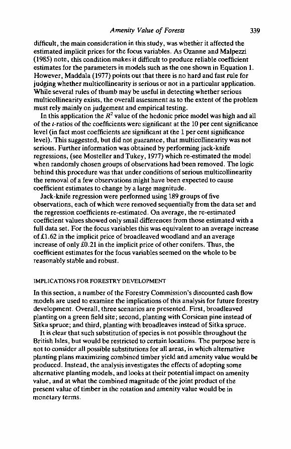
Amenity Value of Forests 339

difficult, the main consideration in this study, was whether it affected theestimated implicit prices for the focus variables. As Ozanne and Malpezzi(1985) note, this condition makes it difficult to produce reliable coefficientestimates for the parameters in models such as the one shown in Equation 1.However, Maddala (1977) points out that there is no hard and fast rule forjudging whether multicollinearity is serious or not in a particular application.While several rules of thumb may be useful in detecting whether seriousmulticollinearity exists, the overall assessment as to the extent of the problemmust rely mainly on judgement and empirical testing.

In this application the R2 value of the hedonic price model was high and allof the f-ratios of the coefficients were significant at the 10 per cent significancelevel (in fact most coefficients are significant at the 1 per cent significancelevel). This suggested, but did not guarantee, that multicollinearity was notserious. Further information was obtained by performing jack-kniferegressions, (see Mosteller and Tukey, 1977) which re-estimated the modelwhen randomly chosen groups of observations had been removed. The logicbehind this procedure was that under conditions of serious multicollinearitythe removal of a few observations might have been expected to causecoefficient estimates to change by a large magnitude.

Jack-knife regression were performed using 189 groups of fiveobservations, each of which were removed sequentially from the data set andthe regression coefficients re-estimated. On average, the re-estimatedcoefficient values showed only small differences from those estimated with afull data set. For the focus variables this was equivalent to an average increaseof £1.62 in the implicit price of broadleaved woodland and an averageincrease of only £0.21 in the implicit price of other conifers. Thus, thecoefficient estimates for the focus variables seemed on the whole to bereasonably stable and robust.

IMPLICATIONS FOR FORESTRY DEVELOPMENT

In this section, a number of the Forestry Commission's discounted cash flowmodels are used to examine the implications of this analysis for future forestrydevelopment. Overall, three scenarios are presented. First, broadleavedplanting on a green field site; second, planting with Corsican pine instead ofSitka spruce; and third, planting with broadleaves instead of Sitka spruce.

It is clear that such substitution of species is not possible throughout theBritish Isles, but would be restricted to certain locations. The purpose here isnot to consider all possible substitutions for all areas, in which alternativeplanting plans maximizing combined timber yield and amenity value would beproduced. Instead, the analysis investigates the effects of adopting somealternative planting models, and looks at their potential impact on amenityvalue, and at what the combined magnitude of the joint product of thepresent value of timber in the rotation and amenity value would be inmonetary terms.

340 Forestry

First, consider a greenfield site, with a small amount of existing tree cover,say three or four broadleaved trees covering 50 m2 and conifers covering1000 m2 (i.e. approximately 5 per cent broadleaves and 95 per cent conifertree mix in the area). If 8950 m2 of broadleaved oak are planted and theconifer area remains as before, relative proportions of broadleaves andconifers will now be 90 per cent and 10 per cent respectively, giving an 85 percent relative increase in broadleaved cover. Note that the total area sums toone hectare, so that a typical discounted cash flow forest rotation model canbe applied. However, the amenity valuation is scale independent in the modelpreviously formulated, so that in principle any size of area can be chosen.Assume that low density housing is permitted at the level of, say 1 house perhectare. Roads, the house and any surrounding garden would reduce theamount of forest land in the hectare block by 10 per cent; with commensuratesavings in costs and reductions in revenues from timber. An 85 per centincrease in broadleaved cover, relative to conifers, would increase the valueof the house by £3655 (i.e. a £43 per unit increase).

The impact of this rotation and the addition of amenity value can be seen inTable 2. Although there is a decline in the value of timber production, and inthe internal rate of return (IRR) from 6.5 for Sitka spruce to 3.1 when theland is devoted to broadleaves, the impact of amenity value is to greatlyincrease the IRR. The scale of the impact depends upon when amenity valueis assumed to occur in the rotation. If amenity value accrues 26 years afterinitial planting, then the IRR increases to 6.7 per cent; but if it occurs only 16years after planting, then the IRR increases to 11.1 per cent. Even if amenityvalue does not accrue until year 26 in the rotation, the effect of includingamenity value is to more than double the IRR from a broadleaved rotation.Alternative distributions could be considered including gradually increasingvalues over time according to some function. The regression model suggeststhat the impact of broadleaves on house prices occurs irrespective of the ageof the trees; i.e. all broadleaves are significant as a category in total. Thus,amenity benefits could commence at the beginning of the rotation, producingan even higher IRR and net present value (NPV).

The second scenario considers an area of land where Corsican pine isplanted instead of Sitka spruce. The same assumptions apply as in theprevious scenario: Corsican pine tree cover increases by 85 per cent relativeto Sitka spruce. Under this scenario the NPV of timber (wood) and the IRRare slightly less than that which would have occurred if the area had beenplanted with Sitka spruce. However, house prices increase by approximately£141 for every unit increase in Corsican pine relative to Sitka spruce (allaccruing through not planting Sitka spruce). The regression model revealsthat amenity value accrues because of old mature Corsican pine, and thiswould occur at the end of the rotation. However, since amenity value isassociated with mature trees, this precludes felling. Thus, under this scenario,the IRR is only marginally higher than that for Sitka spruce. Nevertheless,this does indicate that Corsican pine can be grown as profitably for amenity

Amenity Value of Forests 341

TABLE 2: Amenity and timber values of certain types of forest at 1988 prices(£s)

Base case:Sitka spruce,yield class 16 wood wood + a50 wood + a26 wood + a l6 wood + aO

IRR 6.6NPV 705

Scenario 1:Broadleaved plantingon greenfieldsite,oak, yield class 6

IRR 3.1 4.4 6.7 11.1 •NPV -537 -202 419 1222 3118

Scenario 2:Corsican pine, yieldclass 14, replacesSitka spruce

IRR 6.4 6.7 -NPV 570 1138 -

Scenario 3:Broadleaved, oak,yield class 6,replaces Sitka spruce

IRR 3.1 6.7 12.4 22.8NPV -537 911 3910 7068 15273

aO = amenity value accruing immediately after initial plantingal6 = amenity value accruing 16 years after initial plantinga26 = amenity value acrruing 26 years after initial plantinga50 = amenity value accruing 50 years after initial plantingIRR = internal rate of returnNPV = net present value* = IRR canot be determined

values as Sitka spruce can for timber value!In the third scenario, the proportion of broadleaves is assumed to increase

relative to Sitka spruce. The only difference between scenarios 1 and 3 is theadditional gains which are derived in respect of house prices from deliberatelynot planting Sitka spruce. Again, the same assumptions apply as under thefirst scenario with respect to hectare block and housing. However, amenityvalue under this scenario increases by around £184 for every relative unitincrease in broadleaves: the saving of the £141 decrease in house prices perrelative unit reduction in Sitka spruce, plus the £43 increase per relative unitfrom broadleaves (compared with the Corsican pine, Scots pine and larchcase). Thus, the IRR increases dramatically under the scenario with theinclusion of amenity value. Indeed the combined timber and amenity value is

342 . Forestry

much greater under this scenario than under the Corsican pine model, or thevalue of oak on a greenfield site.

CONCLUSION

The model developed in this paper suggests that the impact of woodland onhousing values may be significant. However, this conclusion can only bedrawn tentatively, since while the hedonic price model can be a useful aid orguide to understanding the value of particular environmental attributes, theaccuracy of any valuation depends upon the satisfaction of the assumptionsunderlying the hedonic price model; and particular problems are encounteredin the case of forestry (Price, 1978,1990). Tree environments are difficult todefine: the layout, shape and size of planting and its relationship to thesurrounding landscape is not easily quantifiable, but this combination cannevertheless potentially affect an individual's valuation. In addition,multicollinearity between tree variables in the sample may result in a loss ofinformation about the specific effect of certain tree types, with theconsequence that only more general results are reportable.

In addition, the data set used in this study only covers Forestry Commissionholdings and does not encompass any private woodland nor any isolated non-commercial trees. Because of this, it was not possible to truly model the'without forestry' case, and consequently the results only measure theenvironmental impact of changes in the relative proportion of ForestryCommission forested area.

Furthermore, because of multicollinearity problems only the effect onhouse prices of changes in three types of tree cover could be investigated.This is a serious limitation, because it means that the effects of a largepercentage of Forestry Commission forested area on house prices are ignoredand may influence the estimated effects of the three classes of woodlandwhich are investigated. The three classes investigated were: all broadleavedtrees; larch, Scots pine and Corsican pine planted before 1920; and all otherconifers (excluding larch, Scots pine and Corsican pine) planted before 1940.

Overall it was found that mature Sitka spruce depressed house prices,ceteris paribus, by approximately £141 for every unit increase in relativecover, while broadleaved trees added approximately £43 per unit increase inrelative cover, in both cases with respect to larch, Scots pine, Corsican pineand other younger conifers. If mature (pre-1920) larch, Scots pine andCorsican pine enter the model they are found to add £20 to house prices forevery unit increase in relative cover. The addition of this tree category, thestatistical effect of which is not significant, alters the values shown above forbroadleaves and mature conifers to an increase of £49 and a reduction of £166respectively. These values are then used to drive the discounted cash flowmodels.

These findings suggest that considerable amenity value can be derived fromplanting broadleaves as opposed to Sitka spruce and other conifers. However,

Amenity Value of Forests 343

the increases in house price that the model suggests might be brought aboutby expanding the relative proportion of broadleaves, would not produce largeenvironmental benefits per property. However, with several of properties inthe same 1 km square, the aggregate impact in terms of extra price and profitfor developers could be large.

A further substantial increase in environmental benefits could be achievedby decreasing the relative proportions of Sitka spruce and other matureconifers more than 50 years old near residential properties or areas, whenfelling and restocking. Replanting with Scots pine, Corsican pine and larchwould reduce environmental disamenities, and produce amenity values asgreat as the value of timber lost from not planting Sitka spruce.

The aggregate wood and amenity value scenario which produces thehighest IRR and largest NPV is the one in which Sitka spruce is replaced bybroadleaved oaks. Such a scenario would be possible in a number of areas inBritain; indeed many ancient woods in upland areas were characterized bypopulations of oak, ash, lime and birch. However, the benefits from such abroadleaved rotation would be mainly in terms of amenity value, a publicgood, flowing to other actors in the countryside rather than to the ForestryCommission.

Such an outcome suggests that there is at present scant incentive for theForestry Commission to plant more broadleaved trees. However, partnershipschemes, or the Forestry Commission itself engaging in housing developmenton land it owns in rural areas would overcome this problem of some of thebenefits produced by one economic agent accruing to another. Indeed, apolicy of permitting limited residential development within the design ofurban woodlands would capture some of the amenity benefits of forestrywhile improving the supply of housing in areas where demand is high.

Nevertheless, the income elasticity of demand for broadleaved trees is nothigh (Garrod and Willis, 1991), and future growth in income is unlikely tolead to a large increase in demand for broadleaved woodland. However, theexpected growth in demand is significantly higher than that for somealternative land uses such as agriculture; while the amenity value ofbroadleaves is significantly greater than timber revenue from Sitka spruce.

The impact of trees on property values reported here are of the same orderof magnitude as those produced by other studies. In the USA Morales (1980)sampled those houses in Amherst, Massachusetts which had a substantialamount of tree cover. After standardizing for other variables affecting houseprice, such as number of rooms, number of bedrooms, number of bathrooms,floor area, garden, age, lot size, etc. trees were estimated to add 6 per cent tothe value of the houses observed. In another study, this time of 844 singlefamily residential house sales in Athens, Georgia, Anderson and Cordell(1988) found that landscaping with trees increased sales prices by 3.5-4.5 percent; a study valuing countryside characteristics in the Forest of Dean and thesurrounding area (Garrod and Willis, 1992) estimated that the proximity ofwoodland cover added approximately 7 per cent to house prices.

344 Forestry

Thus, while there is ample evidence to suggest that woodland may have asignificant influence on housing values, more work is needed to determine thescale and nature of the effect. Further research could usefully be addressed tothe particular problems involved in a hedonic house price study focusing onwoodland environments. This would permit more refined valuations by treetype, age, mix, and design effects to be estimated; and allow comparisons ofthe results from hedonic price methods of the amenity value of trees, withestimates produced by contingent valuation methods or from the opinion ofestate agents with an 'expert' knowledge of housing markets.

ACKNOWLEDGEMENTS

We are grateful to the Nationwide Anglia Building Society for permission touse data on individual house price transactions and to Jim Dewar, SilvicultureDivision, and Adrian Whiteman, Development Division of the ForestryCommission for their help in providing forestry data. Helpful comments wereprovided by Colin Price in reviewing this article. Research for this paper wassupported by the ESRC under the Countryside Change Initiative (Award No.W104251008). The views expressed in this article are those of the authorsalone.

REFERENCES

Anderson, L. M. and Cordell, H. K. 1988 Influence of trees on residential propertyvalues in Athens, Georgia (USA): a survey based on actual sales prices. LandscapeUrban Plann. 15,153-164.

Butler, R. 1982 The specification of hedonic indexes for urban housing. Land Econ.58,96-108.

Cassel, E. and Mendelsohn, R. 1985 The choice of functional forms for hedonic priceequations: comment. J. Urban Econ. 18,135-142.

Cobb, S. 1984 The impact of site characteristics on housing cost estimates. J. UrbanEcon. 15, 26-45.

Cropper, M. L., Deck, L. B. and McConnell, K. E. 1988 On the choice of functionalforms of hedonic price functions. Rev. Econ. Statist. 70, 668-675.

Follain, J., Ozanne, L. and Alburger, V. 1979 Place to Place Indexes of the Price ofHousing. Urban Institute, Washington D.C.

Garrod, G. D. and Willis, K. G. 1991 The environmental economic impact ofwoodland: a two-stage hedonic price model of the amenity value of forestry inBritain. Countryside Change Initiative, Working Paper 19. Department ofAgricultural Economics and Food Marketing, University of Newcastle upon Tyne.

Garrod, G. D. and Willis, K. G. 1992 Valuing Goods' Characteristics: AnApplication of the Hedonic Price Method to Environmental Attributes. J. Environ.Mgmt 34, 59-76.

House of Commons' Committee of Public Accounts 1987 Forestry Commission:Review of Objectives and Achievements. Twelfth Report of the Committee of PublicAccounts for the Session 1986-87. HMSO, London.

Maddala, G. S. 1977 Econometrics. McGraw-Hill International, New York.Morales, D. J. 1980 The contribution of trees to residential property value. /. Arboric.

6, 305-308.

Amenity Value of Forests 345

Mosteller, F. and Tukey, J. W. 1977 Data Analysis and Regression. Addison-Wesley,Reading, MA.

National Audit Office 1986 Review of Forestry Commission Objectives andAchievements. HMSO, London.

Nicholson, M. and Willis, K. G. 1991 Costs and benefits of housing subsidies totenants from voluntary and involuntary rent control: a comparison between tenuresand income groups. Appl. Econ. 23,1103-1115.

Ozanne, L. and Malpezzi, S. 1985 The efficacy of hedonic estimation with the annualhousing survey. / . Econ. Social Measmt 13,153-172.

Price, C. 1978 Landscape Economics. Macmillan, London.Price, C. 1990 Forest Landscape Evaluation. Paper presented to a Forestry

Commission Economics Research Group Meeting in September 1990 at Universityof York.

Willis, K. G. and Benson, J. F. 1989 Recreational value of Forests. Forestry 62,93-110.

Willis, K. G. 1991 Recreational value of the Forestry Commission Estate in GreatBritain. Scott. J. Political Econ. 38, 58-75.

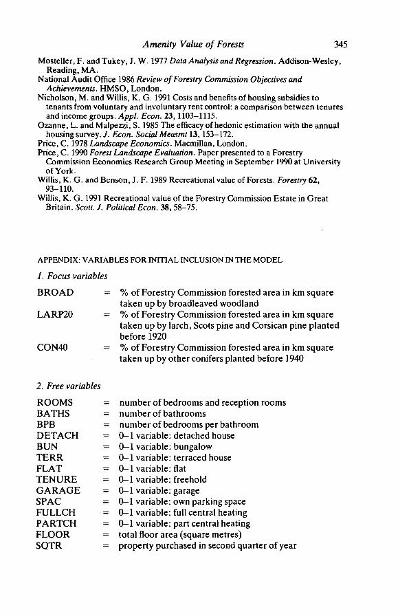
APPENDIX: VARIABLES FOR INITIAL INCLUSION IN THE MODEL

1. Focus variables

BROAD

LARP20

CON40

% of Forestry Commission forested area in km squaretaken up by broadleaved woodland% of Forestry Commission forested area in km squaretaken up by larch, Scots pine and Corsican pine plantedbefore 1920% of Forestry Commission forested area in km squaretaken up by other conifers planted before 1940

2. Free variables

ROOMSBATHSBPBDETACHBUNTERRFLATTENUREGARAGESPACFULLCHPARTCHFLOORSQTR

number of bedrooms and reception roomsnumber of bathroomsnumber of bedrooms per bathroom0-1 variable: detached house0-1 variable: bungalow0-1 variable: terraced house0-1 variable: flat0-1 variable: freehold0-1 variable: garage0-1 variable: own parking space0-1 variable: full central heating0-1 variable: part central heatingtotal floor area (square metres)property purchased in second quarter of year

346 Forestry

TQTR = property purchased in third quarter of yearLQTR = property purchased in fourth quarter of yearBMKT1 = 0-1 variable: property has sitting tenantBMKT2 = 0-1 variable: property is council ownedBMKT8 = 0-1 variable: property requires improvementsBMKTRM = 0-1 variable: property sold below market value for other

reasons

3. Other variables

DIST4

DIST6DIST7DIST10

DIST11

DIST12POPLNRETDPROF

2CARSNOCARUNEMAGRIC

0-1 variable: property in the East Anglian region ofEngland0-1 variable: property in Wales0-1 variable: property in Scotland0-1 variable: property in the East Midlands region ofEngland0-1 variable: property in the Outer Metropolitan regionof Southern England0-1 variable: property in the Northern region of Englandpopulation density of LADpopulation over 60 years of age in LAD (%)population in professional or managerial positions inLAD (%)households with two or more cars in LAD (%)households with no cars in LAD (%)yearly proportion of workforce unemployed in LAD (%)yearly proportion of workforce in agriculture in LAD (%)