POWER OF MEDIAN RTS 1 Another Warning about ... - OSF
40
DRAFT POWER OF MEDIAN RTS 1 Another Warning about Median Reaction Time Jeff Miller Department of Psychology University of Otago Please address editorial correspondence to: Jeff Miller, Department of Psychology, University of Otago, PO Box 56, Dunedin 9054, New Zealand. International FAX: 64-3-479-8335. email: [email protected]. Version of January 19, 2022. Author Note Address correspondence to Jeff Miller, Department of Psychology, University of Otago, Dunedin, New Zealand. Electronic mail may be sent to [email protected]. Revised version of manuscript submitted to Meta-Psychology. Click here to follow the fully transparent editorial process of this submission. Participate in open peer review by commenting through hypothes.is directly on this preprint.
-
Upload
khangminh22 -
Category
Documents
-
view
1 -
download
0
Transcript of POWER OF MEDIAN RTS 1 Another Warning about ... - OSF

DRAFT
POWER OF MEDIAN RTS 1
Another Warning about Median Reaction Time
Jeff Miller
Department of Psychology
University of Otago
Please address editorial correspondence to: Jeff Miller, Department of Psychology,
University of Otago, PO Box 56, Dunedin 9054, New Zealand.
International FAX: 64-3-479-8335.
email: [email protected].
Version of January 19, 2022.
Author Note
Address correspondence to Jeff Miller, Department of Psychology, University of
Otago, Dunedin, New Zealand. Electronic mail may be sent to [email protected].
Revised version of manuscript submitted to Meta-Psychology. Click here to
follow the fully transparent editorial process of this submission. Participate in open
peer review by commenting through hypothes.is directly on this preprint.

POWER OF MEDIAN RTS 2
Abstract
Contrary to the warning of Miller (1988), Rousselet and Wilcox (2020) argued that it is
better to summarize each participant’s single-trial reaction times (RTs) in a given
condition with the median than with the mean when comparing the central tendencies
of RT distributions across experimental conditions. They acknowledged that median
RTs can produce inflated Type I error rates when conditions differ in the number of
trials tested, consistent with Miller’s warning, but they showed that the bias responsible
for this error rate inflation could be eliminated with a bootstrap bias correction
technique. The present simulations extend their analysis by examining the power of
bias-corrected medians to detect true experimental effects and by comparing this power
with the power of analyses using means and regular medians. Unfortunately, although
bias-corrected medians solve the problem of inflated Type I error rates, their power is
lower than that of means or regular medians in many realistic situations. In addition,
even when conditions do not differ in the number of trials tested, the power of tests
(e.g., t-tests) is generally lower using medians rather than means as the summary
measures. Thus, the present simulations demonstrate that summary means will often
provide the most powerful test for differences between conditions, and they show what
aspects of the RT distributions determine the size of the power advantage for means.

POWER OF MEDIAN RTS 3
Another Warning about Median Reaction Time
In typical reaction time (RT) experiments, researchers collect many RTs per
participant in each condition that are then compared via repeated-measures t-tests or
ANOVAs. When they want to determine whether the central tendencies of the RTs
differ between conditions, they are faced with the problem of how to summarize the
many within-condition RTs per participant into a single number for use in the
repeated-measures test. Various summary measures have been used for this
purpose—most commonly the means and medians of the within-condition RTs for each
participant.
Miller (1988) warned that when RT distributions are skewed, as they usually are,
median RTs are biased. Furthermore, this bias is larger when the number of trials per
condition is small. He therefore recommended that medians should not be used when
comparing conditions with different numbers of trials, because the larger bias could
cause conditions with fewer trials to appear slower, even with identical RT distributions
in both conditions. Rousselet and Wilcox (2020; henceforth, R&W) recently disputed
this recommendation based on an extensive series of simulations examining means,
medians, and several other summary measures. In particular, they used a standard
percentile bias correction procedure (e.g., Efron, 1979; Efron & Tibshirani, 1993) and
found that it successfully eliminated the bias problem identified by Miller (1988). In
brief, their procedure estimates the median bias as the difference between the observed
median and the average median across many bootstrap samples. The observed median
is then corrected by subtracting this estimated bias, and the final result of this
subtraction is taken as the bias-corrected median estimate (for further details, see
Rousselet & Wilcox, 2020). In view of the fact that the correction procedure eliminated
median bias and other aspects of their analysis, R&W concluded that “the
recommendation by Miller (1988) to not use the median when comparing distributions
that differ in sample size was ill-advised” (p. 31). Their conclusions have been
influential in encouraging researchers to analyze median RTs (e.g., Gordon et al., 2020;
Maksimenko et al., 2019; Thornton & Zdravković, 2020).
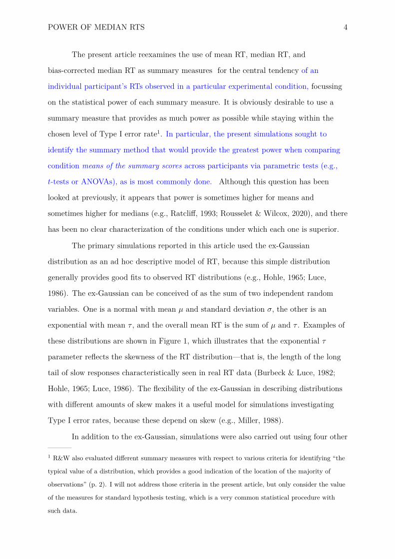
POWER OF MEDIAN RTS 4
The present article reexamines the use of mean RT, median RT, and
bias-corrected median RT as summary measures for the central tendency of an
individual participant’s RTs observed in a particular experimental condition, focussing
on the statistical power of each summary measure. It is obviously desirable to use a
summary measure that provides as much power as possible while staying within the
chosen level of Type I error rate1. In particular, the present simulations sought to
identify the summary method that would provide the greatest power when comparing
condition means of the summary scores across participants via parametric tests (e.g.,
t-tests or ANOVAs), as is most commonly done. Although this question has been
looked at previously, it appears that power is sometimes higher for means and
sometimes higher for medians (e.g., Ratcliff, 1993; Rousselet & Wilcox, 2020), and there
has been no clear characterization of the conditions under which each one is superior.
The primary simulations reported in this article used the ex-Gaussian
distribution as an ad hoc descriptive model of RT, because this simple distribution
generally provides good fits to observed RT distributions (e.g., Hohle, 1965; Luce,
1986). The ex-Gaussian can be conceived of as the sum of two independent random
variables. One is a normal with mean µ and standard deviation σ, the other is an
exponential with mean τ , and the overall mean RT is the sum of µ and τ . Examples of
these distributions are shown in Figure 1, which illustrates that the exponential τ
parameter reflects the skewness of the RT distribution—that is, the length of the long
tail of slow responses characteristically seen in real RT data (Burbeck & Luce, 1982;
Hohle, 1965; Luce, 1986). The flexibility of the ex-Gaussian in describing distributions
with different amounts of skew makes it a useful model for simulations investigating
Type I error rates, because these depend on skew (e.g., Miller, 1988).
In addition to the ex-Gaussian, simulations were also carried out using four other
1 R&W also evaluated different summary measures with respect to various criteria for identifying “the
typical value of a distribution, which provides a good indication of the location of the majority of
observations” (p. 2). I will not address those criteria in the present article, but only consider the value
of the measures for standard hypothesis testing, which is a very common statistical procedure with
such data.

POWER OF MEDIAN RTS 5
statistical models for RT distributions in order to make sure that the obtained results
were not idiosyncratic to the ex-Gaussian. Specifically, these were the ex-Wald
distribution (e.g., Schwarz, 2001), the shifted lognormal distribution, the shifted gamma
distribution, and the three-parameter (i.e., shifted) Weibull distribution. As is
illustrated with the examples in Figure 2, these are all similar to observed RT
distributions in that they are skewed with a long tail at the high end. For each of the
different ex-Gaussian distributions that we examined, parallel simulations of 1,000
experiments were also carried out with each of these alternative distributional models.
For these parallel simulations, the parameters of each alternative distribution were
adjusted so that the alternative distribution matched the corresponding ex-Gaussian at
the 5th, 50th, and 95th percentile points, so we will refer to these as the
“percentile-matched” distributions. To foreshadow the results, the patterns obtained
with all of these percentile-matched distributions closely matched the presented
patterns obtained with the ex-Gaussian. More specifically, although the relative
performance of the mean, median, and bias-corrected median summary measures
depends strongly on RT skewness, it depends hardly at all on the precise underlying
distribution family producing that skewness.
The ex-Gaussian and other skewed distributions are helpful not only in
describing single RT distributions but even more so in describing the effects of
experimental manipulations on these distributions. Observed RT distributions can
easily differ in ways that are too complex to summarize in a single measure of central
tendency such as a mean, so other descriptors of distributional changes can provide
useful clues about the causes of experimental effects (e.g., Balota & Yap, 2011; Balota,
Yap, Cortese, & Watson, 2008; Heathcote, Popiel, & Mewhort, 1991). Besides being of
interest in their own right, these distributional differences may also have implications
for the choice of the most appropriate measure of central tendency to be used when that
is the research focus. One possibility, illustrated by the pair of ex-Gaussians on the left
of Figure 1, is that the experimental manipulation shifts the distribution to the right in
the slower condition, which is described within the ex-Gaussian model by an increase in

POWER OF MEDIAN RTS 6
the µ parameter with no change in skewness. For example, using a spatial Simon
paradigm (e.g., Hommel, 2011), Luo and Proctor (2018) asked participants in their
Experiment 1 to respond with the left versus right hand to red versus green squares
that appeared irrelevantly to the left or right of fixation. Even though location was
irrelevant, responses were faster when the square appeared on the same side as the
required response than when it appeared on the opposite side. At the distributional
level, this RT difference was well described as a shift effect reflected entirely in the µ
parameter, with no change in skewness (τ). Another possibility, illustrated by the pair
of ex-Gaussians on the right side of Figure 1, is that the experimental manipulation
stretches the tail of the RT distribution in the slower condition, essentially increasing its
skew, which can be described as an effect that is entirely on τ . For example, in their
Experiment 3, Luo and Proctor (2018) asked participants to respond with the left
versus right hand to red versus green arrows that pointed irrelevantly to the left or
right, and responses were faster when the arrow pointed to the same side as the
required response than when it pointed to the opposite side. This time, however, the
RT difference was mainly due to a stretched tail, with increased skew reflected in a
larger τ , and there was little change in µ.
Since the introduction of the ex-Gaussian by Hohle (1965), many studies have
examined the shifting versus tail-stretching effects of various experimental
manipulations on the shapes of RT distributions as described in terms of µ and τ . Both
µ and τ are typically larger in the slower condition than in the faster one, indicating
that most experimental manipulations have both shifting and stretching effects, in
varying mixtures. There is unfortunately no consensus about the psychological
meanings of changes in these different parameters, because there are at best weak
distinctions between experimental manipulations with shifting versus stretching effects
(e.g., Matzke & Wagenmakers, 2009; Rieger & Miller, 2020), but the ex-Gaussian
distribution nevertheless remains useful as a way of describing changes in the shapes of
RT distributions as well as their means. For the present purposes, the distinction
between shifting and stretching effects is relevant because—as will be seen—statistical

POWER OF MEDIAN RTS 7
tests based on means, medians, and bias-corrected medians are especially different in
their power to detect stretching effects.
Type I Error Rates
For completeness, and to make the simulation process more concrete, this section
reviews briefly the well-established fact that Type I error rates are inflated by
sample-size-dependent bias when medians are used to compare RTs across conditions
with unequal numbers of trials (which I will call unequal trial “frequencies” rather than
“sample size”, to avoid confusion with the number of participants). This bias is an
artifact that would contaminate comparisons of conditions with different trial
frequencies if medians were used to summarize the RTs in each condition. Originally,
comparisons of such conditions were used particularly in studies of the main effects of
stimulus and response probability (e.g., Hyman, 1953), attentional cuing (e.g., Posner,
Nissen, & Ogden, 1978), and expectancy (e.g., Mowrer, Rayman, & Bliss, 1940; Zahn &
Rosenthal, 1966). In addition, trial frequencies have often been varied across conditions
to explore a variety of cognitive processes by investigating their interactions with
probability (e.g., Broadbent & Gregory, 1965; Den Heyer, Briand, & Dannenbring,
1983; Miller & Pachella, 1973; Sanders, 1970; Theios, Smith, Haviland, Traupmann, &
Moy, 1973). Currently, trial frequencies are commonly varied in studies of spatial and
temporal statistical learning (e.g., Flowers, Palitsky, Sullivan, & Peterson, 2021; Gibson,
Pauszek, Trost, & Wenger, 2021; Liesefeld & Müller, 2021; Vadillo, Giménez-Fernández,
Beesley, Shanks, & Luque, 2021), the modulation of attentional control processes by
environmental contingencies (e.g., Cochrane, Simmering, & Green, 2021; Huang,
Theeuwes, & Donk, 2021; Kang & Chiu, 2021), action-outcome contingency learning
(e.g., Gao & Gozli, 2021), adaptation to the frequency of congruent versus incongruent
information (e.g., Bausenhart, Ulrich, & Miller, 2021; Ivanov & Theeuwes, 2021;
Thomson, Simone, & Watter, 2021), and between-task resource sharing (e.g., Miller &
Tang, 2021), to name just a few areas. Unfortunately, median bias is still sometimes
overlooked and may contaminate published comparisons of conditions with different

POWER OF MEDIAN RTS 8
trial frequencies (e.g., Bulger, Shinn-Cunningham, & Noyce, 2021).
As noted by Miller (1988) and confirmed by R&W’s Table 2, sample medians are
biased with skewed distributions, and the bias is greater when the number of trials is
smaller. If medians are used to compare conditions with different trial frequencies, this
bias causes the Type I error rate to be inflated—perhaps seriously. Specifically, the
low-frequency condition will often appear to be statistically slower than the
high-frequency condition, even if the true RT distributions are identical in the two
conditions.
A simple simulation of 5,000 experiments illustrates the problem. In each
simulated experiment, RTs were generated for 60 participants. Each participant was
tested for 51 trials in the “frequent” condition and 5 trials in the “infrequent”
condition, with odd numbers of trials used so that the median of each sample would be
the unique middle score. The null hypothesis was always true—that is, RTs for both
conditions were sampled from the same underlying ex-Gaussian distribution with
µ = 400, σ = 50, τ = 200 shown in Figure 1. Within each simulated experiment, the
RTs sampled for each participant were summarized by computing the median in each
condition. Using these medians as the dependent variable, a paired t-test comparing the
means of these medians was then computed across the 60 participants, with α = 0.05,
two-tailed. Since the null hypothesis was true in the simulated experiments, one would
theoretically expect approximately 5% significant results (i.e., Type I errors) by chance,
with half of these yielding significantly larger scores in the frequent condition and half
significantly larger scores in the infrequent condition. However, the simulation actually
produced 17.8% Type I errors where the infrequent condition appeared slower versus
only 0.1% where the frequent condition appeared slower. Thus, in accordance with the
warning of Miller (1988), comparing the means of participant/condition median RTs
produced far too many Type I errors in the direction that would lead researchers to
conclude that responses are slower in the infrequent condition.
The inflated Type I error rate for medians arises for purely statistical reasons.
As is described in the Appendix, the full sampling distribution of the sample medians

POWER OF MEDIAN RTS 9
can be computed numerically using the known properties of order statistics (i.e., the
median of the smaller sample is the third order statistic in a sample of five, and the
median of the larger sample is the 26th order statistic in a sample of 51), and these
sampling distributions are shown in Figure 3. Crucially, the means of these sampling
distributions are 561.4 and 546.7, respectively, so the long-run mean of the smaller
sample medians really is larger than that of the larger samples. The t-test results
simply reflect this true difference in average medians for samples of these two sizes from
this distribution. In comparison, across exactly the same simulated datasets using each
participant’s condition mean or bias-corrected median2 as the summary measure,
approximately 2.5% Type I errors in each direction were obtained, as expected.
Parallel simulations were carried out to determine the extent of error rate
inflation under a variety of different simulation conditions, and representative results
are shown in Figure 4. The different simulation conditions used: (a) varying numbers of
trials N in the infrequent condition (the frequent condition always had 51 trials), as
shown along the horizontal axis; (b) ex-Gaussian (or corresponding percentile-matched
distributions) with different values of µ and τ to vary the degree of skewness, shown as
different lines; and (c) 30 or 60 participants in the experiment, shown in the panels on
the left or right. The vertical axis shows the proportion of simulated experiments in
which researchers would reject the null hypothesis and conclude that responses were
slower in the infrequent condition. Since scores in both conditions were actually always
drawn from the same distribution, these would again be Type I errors in that direction.
Obviously, the Type I error rates for the median analyses can far exceed the appropriate
2.5% with small Ns in the infrequent condition, whereas the error rates for the means
do not. Bias-corrected medians also produced appropriate error rates, replicating
R&W’s results.
Very similar patterns of Type I error rates were obtained in the simulations with
the other four percentile-matched distributions used as RT models (i.e., ex-Wald,
shifted lognormal, etc). For example, across the 32 simulation conditions shown in
2 For all simulations in this article, bias-corrected medians were based on 200 bootstrap samples.

POWER OF MEDIAN RTS 10
Figure 4, the average Type I error rate for the median was 6.7% for the ex-Gaussian,
whereas it ranged from 6.1% to 6.7% with the other four distributions. Similarly, the
Type I error rate exceeded 15% for all distributions in the worst case (i.e., the
simulation with 60 participants, five trials in the infrequent condition, and the
most-skewed distribution percentile-matched to the ex-Gaussian with µ = 350 and
τ = 250). Meanwhile, the Type I error rates for the mean and bias-corrected medians
were always around 2% for these other distributions, just as they were with the
ex-Gaussian (Fig. 4). Thus, the finding of inflated Type I errors for medians seems
relatively independent of the precise shape of the skewed RT distribution.
The simulations presented so far have all used pure, uncontaminated RT
distributions, but there are reasons to suspect that observed RT distributions contain
occasional outliers (e.g., Ratcliff, 1993; Ulrich & Miller, 1994), perhaps because the
participant’s attention momentarily wanders away from the task. It is an empirical
question whether the results shown in Figure 4 would change markedly if the simulations
included outliers. For example, since means are more affected by extreme scores than
medians, the Type I error rates associated with mean-based analyses might be inflated
when outliers are included. To look at the effects of outliers, additional simulations were
conducted using each of the different RT models already introduced. These simulations
included either 2% or 4% outliers, and the outliers were formed by summing an RT
from the uncontaminated distribution with a random number distributed uniformly
between 0–1,000 ms to reflect a distraction delay3. Such outliers had hardly any
influence on the Type I error rates obtained using means, medians, or bias-corrected
medians, so it seems unlikely that outliers in real RT data would reduce the Type I
error rate advantage for means and bias-corrected medians relative to regular medians.
R&W acknowledged the problem of inflated Type I errors when using sample
medians for comparing population means (e.g., with t-tests), and their Figure 10B even
3 Ratcliff (1993) introduced outliers varying uniformly between 0–2,000 ms, but it seems that responses
delayed by 1,000–2,000 ms would be easily identified and excluded by commonly-used outlier rejection
techniques.

POWER OF MEDIAN RTS 11
shows simulation results displaying the problem. Nonetheless, they essentially dismissed
this problem because “the bias can be strongly attenuated by using a percentile
bootstrap bias correction” (p. 31), which is a procedure that was not considered by
Miller (1988). Indeed, their Figure 10C shows that the bootstrap bias correction
completely cures the Type I error rate problem, as is also shown in the present Figure 4.
Thus, it is reasonable to consider the bias-corrected median as a possible summary
measure of RTs, and the next step is to check its power.
Power
Given that bias correction solves the median’s problem of Type I error rate
inflation, it is tempting to suspect that bias-corrected medians would be preferable to
means, because the median is often the preferred measure of central tendency with
skewed distributions. Contrary to this intuition, however, Ratcliff (1993) reported that
regular medians provide less statistical power than means. R&W acknowledged
Ratcliff’s report, but they downplayed it because of the small trial frequencies used in
Ratcliff’s analysis. In addition, it remains an open question how the power of
bias-corrected medians compares with that of means. The present simulations
investigated these issues.
Fortunately, it is easy to compare the power of means versus bias-corrected
medians using simulations similar to those described above for assessing Type I error
rate. Instead of using the same RT distributions for the two conditions being compared,
one simply uses different distributions and checks the proportion of simulated
experiments yielding a statistically significant difference—this proportion is an estimate
of statistical power. To model the different types of experimental effects for which
researchers might test, one can allocate different amounts of the RT increase in the
slower condition to different amounts of shifting versus skewing (i.e., tail-stretching)
effects on the RT distribution. Within the ex-Gaussian RT model this amounts to
increases in the µ versus τ parameters, and changes in other parameters produce
comparable shifting versus stretching effects within the other RT distribution models.

POWER OF MEDIAN RTS 12
The first set of power simulations examined the ability of the different summary
measures to reveal a true between-condition RT difference in experiments where the two
conditions had unequal trial frequencies, and the results of these simulations are
displayed in Figure 5. Regular medians would not be appropriate in this situation
because of the Type I error rate problem described in the previous section, so these
simulations only compared the power of tests using means and bias-corrected medians.
Naturally, these two types of testing were compared under identical simulation
conditions, and in fact identical samples of simulated RTs were always analyzed with
the two summary measures.
In total, there were 32 simulation conditions using ex-Gaussian RT distributions,
corresponding to the 32 points shown in Figure 5, for each of the mean-based and
bias-corrected median-based tests. In all 32 simulation conditions, 51 RTs per
participant were sampled from the faster condition, and the true mean RT in the faster
condition was 600 ms. The 32 conditions were formed as the factorial combination of
eight different dataset sizes and four conditions differing with respect to RT skewness.
The eight dataset sizes consisted of 30 or 60 participants factorially combined with 5, 9,
17, or 33 trials in the slower condition. The four skewness conditions were formed using
two amounts of skewness of the RT distribution in the faster condition (i.e., µf = 350
and τf = 250 or µf = 500 and τf = 100, with σ = 50 in both cases) and by allocating
the RT increase in the slower condition either 25% to µs and 75% to τs, or the reverse4.
Thus, in different simulation conditions the faster RT distribution was either more or
less skewed to begin with and the mean RT difference between conditions arose either
mostly from shifting the distribution in the slower condition or mostly from stretching
it. Finally, the true mean RT difference between the fast and slow conditions was
adjusted individually for each of the 32 simulation conditions to produce an
intermediate power level (i.e., approximately 25%–75%) for tests using means as the
4 In the corresponding 32 simulation conditions using each of the percentile-matched distributions,
adjustments of the parameters of those distributions were made as needed to match the percentiles of
the other distributions to those of the ex-Gaussians used in the fast and slow conditions.

POWER OF MEDIAN RTS 13
summary measure. Intermediate power levels are desirable because they provide the
best opportunity to observe power differences between means and bias-corrected
medians; with very low or high power levels, the differences between analysis methods
are compressed by floor or ceiling effects. Across the 32 simulation conditions, the true
mean difference varied from 9–41 ms.
Not surprisingly, the results shown in Figure 5 indicate that the power of t-test
comparisons increases with the number of participants and the number of trials per
participant, and in fact these power increases are even more dramatic than are shown
because the true differences were adjusted to smaller values with larger datasets in order
to avoid ceiling effects on power. More critically, they also show a clear power advantage
for using means rather than bias-corrected medians. Thus, although the bias-correction
procedure lets the median do as well as the mean with respect to Type I errors (Fig. 4),
this summary measures seems to have much less power than the simpler option of using
means. The advantage for mean-based testing depends little either on the number of
trials in the slower condition or on the skewness of RTs in the faster condition (i.e.,
µf = 350 versus µf = 500). It is clearly larger, however, when the experimental effect
arises mainly from a tail-stretching effect (i.e., ∆µ/∆ = 0.25; upper panels) rather than
from a shifting effect (i.e., ∆µ/∆ = 0.75; lower panels). Indeed, further simulations (not
shown) indicate that the power of mean-based analyses is only slightly higher than that
of analyses using bias-corrected medians when slowing is almost entirely due to a shift
(i.e., ∆µ/∆ = 0.95). The reasons for this pattern will become clearer after the next set
of simulations, which reinforce and extend the pattern.
Once again, the results of the simulations with the other, percentile-matched RT
distributions closely match those of the ex-Gaussian RT distributions, with these
simulations also showing greater power for mean-based testing. For example, across the
32 simulation conditions in Figure 5, the average power levels of the mean- and
bias-corrected median-based tests were 0.58 and 0.32, respectively. With the other
distributions, the average power for means ranged from 0.55–0.58, and the average
power for bias-corrected medians ranged from 0.26–0.31. Similarly, across all

POWER OF MEDIAN RTS 14
distribution types and all simulation conditions, the minimum and maximum power
levels ranged from 0.30–0.37 and 0.77–0.80 respectively for means, whereas these ranges
extended from 0.11–0.12 and 0.51–0.61 for bias-corrected medians. In further
simulations including 2% or 4% outliers of the same type used in the earlier Type I
error rate simulations, power decreased for both mean- and bias-corrected median-based
tests, but average power across simulation conditions was still more than 10% higher for
the mean than for the bias-corrected median with all distributions.
In view of the fact that mean-based RT summaries have demonstrably greater
power than bias-corrected median-based summaries for experiments with unequal trial
frequencies (Fig. 5), it is also sensible to compare power levels in experiments with equal
trial frequencies. As noted by Miller (1988) and R&W, regular medians are not
associated with Type I error rate inflation in this situation because they would be
equally biased in both conditions, so regular medians can also be considered as an
appropriate summary of single-trial RTs in this case. It is, however, useful to compare
the power of these three candidate measures of central tendency (i.e., means, medians,
bias-corrected medians).
Figure 6 shows the results of simulations analogous to those shown in Figure 5,
except with equal numbers of trials per participant in the faster and slower conditions,
and naturally power again increased in the simulation conditions with more participants
and trials even though these conditions had smaller true mean differences to avoid
ceiling effects. Power is consistently lower for bias-corrected medians than for regular
medians, suggesting that the bias correction should not be used with equal trial
frequencies. Mean-based tests again have the most power, although the power difference
between means and medians depends heavily on whether the experimental manipulation
has mostly a shifting or tail-stretching effect. As can be seen in the upper panels of
Figure 6, means have substantially more power than medians when a minority of the
RT difference results from a change in µ (i.e., ∆µ/∆ = 0.25). The power advantage for
means is much reduced when a majority of the RT difference results from a change in µ
(i.e., ∆µ/∆ = 0.75), and medians can actually have slightly more power when the RT

POWER OF MEDIAN RTS 15
difference is a pure shift (i.e., ∆µ/∆ = 1.00; not shown). The same qualitative patterns
are evident in Figs. 14–16 of R&W.
Overall, the pattern of greater power for mean-based testing shown in Figure 6
was again consistent across distributions and outlier conditions. Averaging across the
different dataset sizes and skewness combinations shown in the figure, the average
power levels of mean-based testing ranged across distributions from 0.55–0.58, whereas
the ranges for median- and bias-corrected median-based testing were 0.38–0.45 and
0.27–0.33, respectively. The presence of 2% or 4% outliers reduced these average power
levels overall, but average power was still largest for means (ranging across distributions
from 0.46–0.49 and 0.41–0.43 with 2% and 4% outliers, respectively), second-largest for
medians (ranging from 0.37–0.43 and 0.35–0.41), and smallest for bias-corrected
medians (ranging from 0.26–0.31 and 0.26–0.30).
Why is it that using participant mean RTs as the summary measure has so much
more power when the experimental effect is mostly a stretch in the slow tail? The main
reason is simply that power increases with effect size, as is true for all statistical tests.
Consider two conditions whose true mean RTs differ by 40 ms. In that case, the
expected difference in mean RTs between those two conditions is 40 ms, regardless of
how the effect is distributed between shifting and stretching and regardless of how many
trials there are per participant in each condition. The situation is far more complicated
for differences in medians, however, as is illustrated with the ex-Gaussian distribution in
Figure 7. Figure 7A shows the expected value of the difference between the medians of
the fast and slow conditions (∆mdn) as a function of (a) how much of the 40 ms mean
RT difference is produced by changes in µ versus τ (i.e., ∆µ versus ∆τ ), and (b) how
many trials per participant are tested in each condition5. Critically, the expected
difference between medians is always less than the 40 ms expected difference in means,
and it is far less when the conditions differ mostly in τ (i.e., ∆µ = 10 and ∆τ = 30)
rather than mostly in µ (i.e., ∆µ = 30 and ∆τ = 10), particularly when the number of
5 The results shown in this figure were obtained by computation rather than by simulation, using
methods explained in the Appendix.

POWER OF MEDIAN RTS 16
trials is large. The fact that the numerical differences are larger for means than medians
strongly suggests that tests using means would have more power. In theory, medians
could provide more statistical power despite their smaller effect size in milliseconds if
they had much smaller standard errors. They do not, however, as is clear in Figure 7B,
which shows the corresponding ratios of the standard error of the difference in means to
the standard error of the difference in medians. These ratios are quite close to 1.0,
which means that the standard errors of the means and medians are nearly equal in all
of these cases. Figure 7C shows the comparison of means versus medians plotted in
terms of Cohen’s d, a standard effect size measure. Effect sizes increase with the
number of trials, as expected because the standard error of the sample statistics (i.e.,
mean and median) decrease as the number of trials increases. More importantly, it is
clear that effect sizes are larger for means than for medians across all conditions, and
this is the source of the power advantage for means.
In essence, when much of an experimental manipulation’s effect is to stretch the
long upper tail of the RT distribution, the median’s relative insensitivity to this part of
the distribution eliminates part of the very between-condition difference that the
researcher is looking for6. This is particularly ironic because insensitivity to skew is
often cited as one of the median’s benefits, and it is supposed to make the median
especially tempting with skewed distributions (e.g., Hays, 1973; Marascuilo, 1971). As
noted by Yule (1911), for example, “The median may [italics in original] sometimes be
preferable to the mean, owing to its being less affected by abnormally large or small
values of the variable” (p. 120), although he also commented that the median’s
“limitations render the applications of the median in any work in which theoretical
considerations are necessary comparatively circumscribed” (p. 119). As the present
simulations show, however, means can have much higher power to detect
between-condition RT differences when experimental manipulations increase skewness,
6 The same problem would arise with trimmed means, though to a lesser extent, because trimming also
reduces the contribution of the high end of the RT distribution, where the condition difference is
greatest.
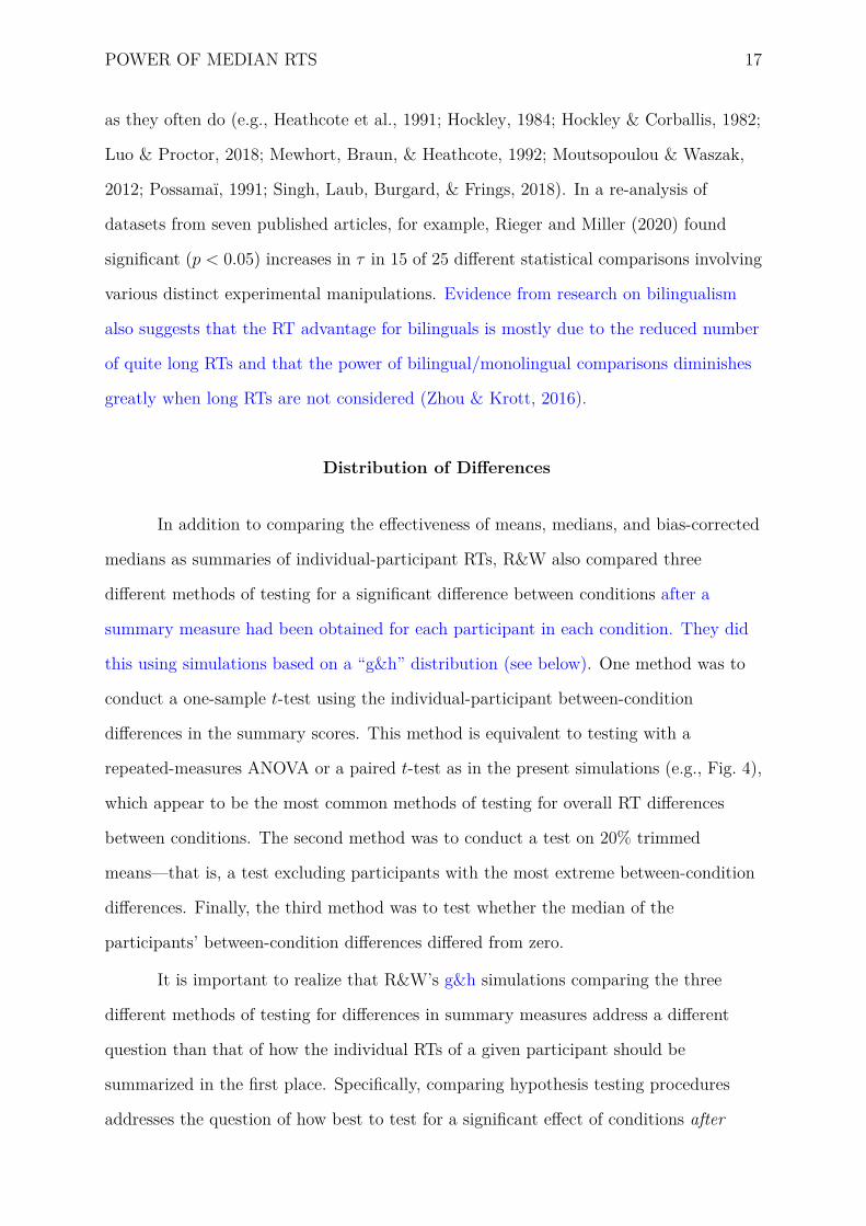
POWER OF MEDIAN RTS 17
as they often do (e.g., Heathcote et al., 1991; Hockley, 1984; Hockley & Corballis, 1982;
Luo & Proctor, 2018; Mewhort, Braun, & Heathcote, 1992; Moutsopoulou & Waszak,
2012; Possamaï, 1991; Singh, Laub, Burgard, & Frings, 2018). In a re-analysis of
datasets from seven published articles, for example, Rieger and Miller (2020) found
significant (p < 0.05) increases in τ in 15 of 25 different statistical comparisons involving
various distinct experimental manipulations. Evidence from research on bilingualism
also suggests that the RT advantage for bilinguals is mostly due to the reduced number
of quite long RTs and that the power of bilingual/monolingual comparisons diminishes
greatly when long RTs are not considered (Zhou & Krott, 2016).
Distribution of Differences
In addition to comparing the effectiveness of means, medians, and bias-corrected
medians as summaries of individual-participant RTs, R&W also compared three
different methods of testing for a significant difference between conditions after a
summary measure had been obtained for each participant in each condition. They did
this using simulations based on a “g&h” distribution (see below). One method was to
conduct a one-sample t-test using the individual-participant between-condition
differences in the summary scores. This method is equivalent to testing with a
repeated-measures ANOVA or a paired t-test as in the present simulations (e.g., Fig. 4),
which appear to be the most common methods of testing for overall RT differences
between conditions. The second method was to conduct a test on 20% trimmed
means—that is, a test excluding participants with the most extreme between-condition
differences. Finally, the third method was to test whether the median of the
participants’ between-condition differences differed from zero.
It is important to realize that R&W’s g&h simulations comparing the three
different methods of testing for differences in summary measures address a different
question than that of how the individual RTs of a given participant should be
summarized in the first place. Specifically, comparing hypothesis testing procedures
addresses the question of how best to test for a significant effect of conditions after

POWER OF MEDIAN RTS 18
summarizing the original individual-participant RTs in each condition. This is a
different question because researchers could initially summarize individual-trial RTs
with any of the summary methods (i.e., means, medians, bias-corrected medians) and
then subsequently test for condition differences with any of the hypothesis testing
methods (i.e., t-test, 20% trimmed means test, median test). In principle, any one of
these nine options could provide the most statistical power. Thus, the conclusions of
the present simulations comparing different summary methods are specific to the t-tests
and these simulations might have a different outcome if the summary measures were
compared across conditions with some other method.
In their comparison of different hypothesis testing procedures using the g&h
distribution, R&W did not distinguish between the three different methods of
summarizing individual-trial RTs (i.e., means, medians, bias-corrected medians). In
fact, they only generated a single random number for each simulated participant, and
this number represented the difference (i.e., condition effect) for that participant
summarized from the individual-participant RTs with “any type of differences between
means, medians or any other quantities” (p. 17). These individual-participant difference
scores were generated from “g&h” distributions, which allow convenient parametric
variation of distribution skewness and kurtosis (i.e., tail heaviness) through g and h
parameters, respectively. Although it might seem more appropriate to simulate
single-trial RTs and examine all nine possible analysis combinations (i.e., 3 summary
methods × 3 hypothesis testing methods), it is not clear how to do that realistically.
Even assuming that all of the individual-participant RT distributions were
ex-Gaussians, the participants would surely differ in their distribution parameters and
in their between-condition differences in these parameters (e.g., effects on µ and τ). The
distribution of individual-participant difference scores would be heavily influenced by
this participant-to-participant variation as well as by the choice of summary method,
but there does not yet exist an appropriate model for this individual variation. Thus, it
was not unreasonable for R&W to model the final distribution of individual-participant
difference scores directly with the g&h distribution rather than attempting to specify a

POWER OF MEDIAN RTS 19
model in which these difference scores would emerge from varying individual RT
distributions under each summary method.
R&W’s simulations comparing the effectiveness of the different hypothesis
testing methods produced two particularly important results (e.g., their Figs. 12 and
13). First, each of the hypothesis testing methods tends to lose power when the
distribution of participant-to-participant difference scores is more skewed or has heavier
tails (i.e., larger kurtosis). Second, this tendency to lose power with increasing skew or
kurtosis is much stronger for the t-test than for the tests using trimmed means or
medians. Naturally, then, R&W suggested that researchers should consider carefully the
amount of skew and kurtosis in their distributions of participant-to-participant
difference scores when deciding which procedure to use in testing for a condition effect.
Although R&W’s simulations comparing hypothesis testing methods do not
speak directly to the question of how the individual-participant RTs should be
summarized in the first place, as was mentioned earlier, one might suspect that they do
so indirectly. In particular, their results suggest that researchers should prefer the
summary measure for which the participant-to-participant difference scores are the least
skewed and have the lightest tails. Intuitively, it might seem reasonable to assume that
medians—by virtue of their smaller sensitivity to extreme scores—would produce
difference score distributions that are less skewed and have lighter tails than those
produced by means, but this assumption must be checked empirically.
To do that, I examined the two large, publicly available RT datasets of Ferrand
et al. (2010) and Hutchison et al. (2013), both involving lexical decision tasks. In both
datasets, responses to words were faster than responses to nonwords, which provided a
convenient condition effect to examine. Since these are real datasets, they have realistic
trial-to-trial RT variability and participant-to-participant variability in condition
effects, by definition, obviating the need to specify a formal model for these. Thus, I
computed three separate nonword-minus-word difference scores for each
participant—once each using the participant’s condition mean RTs, condition median
RTs, and bias-corrected condition median RTs. The normalized frequency distributions

POWER OF MEDIAN RTS 20
of these difference scores for the two datasets, tabulated across 944 and 503
participants, respectively, are shown in Figure 8.
Perhaps somewhat counterintuitively, the empirical distributions of
individual-participant difference scores shown in Figure 8 are both less skewed (smaller
values of skew and g) and lighter tailed (smaller values of kurtosis and h) when the
difference scores are computed from mean RTs than when they are computed from either
of the median-based summary measures. In combination with R&W’s finding of greater
power with less skewed and lighter-tailed difference score distributions, this pattern
provides clear evidence that researchers would have more power when using means
rather than medians to summarize RTs. Based on R&W’s results, it seems that this
would be true regardless of which hypothesis testing procedure was used, but it appears
that the mean advantage would be especially large with standard t-tests or ANOVAs.
A distinctive feature of the SPP and FLP datasets, relative to many published
studies, is that there were unusually many trials in each condition. One might therefore
wonder whether the results shown in Figure 8 would generalize to datasets with fewer
trials per condition (perhaps because there were more conditions). To examine this
issue, I conducted simulations with smaller random subsets of the RTs for each
participant in each condition. To increase the stability of the simulation results, 20
subsets of a given number of RTs were randomly selected for each participant, selecting
without replacement for each subset but with replacement across subsets (because there
were not enough RTs to sample without replacement for the larger subsets). For each
randomly selected subset of RTs from one participant, the condition effect was
computed using each of the three summary measures (i.e., mean, median, bias-corrected
median). Finally, across all simulated subsets for a given number of RTs, the
distribution of condition effects was analyzed using the same computations as those
shown in Figure 8 for the full datasets.
Figure 9 shows the results of these simulations, which nicely extend the results
obtained with hundreds of trials per participant in each condition (Fig. 8) to datasets
with smaller numbers of trials. With virtually any number of trials per condition per

POWER OF MEDIAN RTS 21
participant selected from these real datasets, the between-participant difference score
distributions would be less skewed (i.e., smaller skewness and g) and less heavy-tailed
(i.e., smaller kurtosis and h) when differences were computed from mean RTs than when
they were computed from medians or bias-corrected medians. Thus, as with the full
datasets, these results in combination with R&W’s demonstration of greater power with
less skew and lighter tails, provide a further argument for using the mean to summarize
the central tendency of observed RTs.
Conclusions
R&W concluded that “there seems to be no rationale for preferring the mean
over the median as a measure of central tendency for skewed distributions” (p. 31). On
the contrary, when performing hypothesis tests to compare the central tendencies of
RTs between experimental conditions, the present simulations show that there may be
an extremely clear rationale involving both Type I error rate and experimental power.
When comparing conditions with unequal numbers of trials, the
sample-size-dependent bias of regular medians can lead to clear inflation of the Type I
error rate (Fig. 4), so these medians definitely should not be used. Means and
bias-corrected medians are both free of this bias and thus have acceptable Type I error
rates, so either could be considered as a possible summary measure in this situation.
Means clearly have greater power (Fig. 5) than bias-corrected medians in most
situations, however, which would nearly always make them the preferred choice.
When comparing conditions with equal numbers of trials, means, medians, and
bias-corrected medians all have appropriate Type I error rates, so any of these might be
the preferred summary measure in this situation. Bias-corrected medians always seem
to have less power than regular medians, however, so here the choice is really between
means and regular medians, depending on which of those has the higher power. As can
be seen in Figure 6), the answer depends on how the experimental manipulation affects
skewness. Thus, to choose between means and medians as the summary measure
maximizing power, researchers must consider the effect of the experimental

POWER OF MEDIAN RTS 22
manipulation at the level of the RT distribution.
The results in Figure 6 suggest that the two measures will have approximately
equal power when RT skewness is unaffected by the manipulation, whereas medians will
have greater power if skewness decreases in the slower condition and means will have
greater power if skewness increases in the slower condition. Although the ex-Gaussian τ
is one way of assessing skewness, it is not always necessary to estimate ex-Gaussian
parameters from RT distributions. Instead, one can use a simpler skewness
measure—namely, the difference between the mean and median of RT—as a proxy for
τ . If this difference is smaller in the slower condition than the faster one, that is a sign
that power will be better using medians. On the other hand, if this difference is larger
in the slower condition, power will be better using means.
An important caveat concerning the choice of summary measure is that this
choice should not be made based on the data being analyzed. To avoid the inflation of
Type I error rate that arises when researchers try multiple alternative analyses in the
attempt to obtain significant results (i.e., “p-hacking” Simmons, Nelson, & Simonsohn,
2011), researchers must choose the best summary measure in advance, based on
theoretical considerations regarding the expected effect, on prior experience with similar
experimental manipulations, or on pilot data. It would be inappropriate to decide
whether to analyze mean or median RTs based on whichever gave the larger effect in a
given dataset, because this would inflate the researcher’s Type I error rate.
Acknowledgements
I am grateful to Wolf Schwarz, Patricia Haden, Veronika Lerche, Guillaume
Rousselet, and Rand Wilcox for helpful comments on earlier versions of this article, and
to Ludovic Ferrand for providing the raw data from the French Lexicon Project.
Declaration of Conflicting Interests
The author declares that he had no conflicts of interest with respect to the
authorship or publication of this article.
Code Availability
MATLAB code to conduct the reported simulations is available at the Open

POWER OF MEDIAN RTS 23
Science Foundation project osf.io/yqz6b. The ex-Gaussian, ex-Wald, shifted lognormal,
shifted gamma, and Weibull distributions used in this code are part of the Cupid
package available at https://github.com/milleratotago/Cupid.

POWER OF MEDIAN RTS 24
References
Arnold, B. C., Balakrishnan, N., & Nagaraja, H. N. (1992). A first course in order
statistics. New York, NY: Wiley.
Balota, D. A., & Yap, M. J. (2011). Moving beyond the mean in studies of mental
chronometry: The power of response time distributional analyses. Current
Directions in Psychological Science, 20 (3), 160–166. doi:
10.1177/0963721411408885
Balota, D. A., Yap, M. J., Cortese, M. J., & Watson, J. M. (2008). Beyond mean
response latency: Response time distributional analyses of semantic priming.
Journal of Memory & Language, 59 (4), 495–523. doi: 10.1016/j.jml.2007.10.004
Bausenhart, K. M., Ulrich, R., & Miller, J. O. (2021). Effects of conflict trial
proportion: A comparison of the Eriksen and Simon tasks. Attention, Perception,
& Psychophysics, 83 (2), 810–836. doi: 10.3758/s13414-020-02164-2
Broadbent, D. E., & Gregory, M. H. P. (1965). On the interaction of S-R compatibility
with other variables affecting reaction time. British Journal of Psychology, 56 ,
61–67. doi: 10.1111/j.2044-8295.1965.tb00944.x
Bulger, E., Shinn-Cunningham, B. G., & Noyce, A. L. (2021). Distractor probabilities
modulate flanker task performance. Attention, Perception, & Psychophysics,
83 (2), 866–881. doi: 10.3758/s13414-020-02151-7
Burbeck, S. L., & Luce, R. D. (1982). Evidence from auditory simple reaction times for
both change and level detectors. Perception & Psychophysics, 32 , 117–133. doi:
10.3758/BF03204271
Cochrane, A., Simmering, V., & Green, C. S. (2021). Modulation of compatibility
effects in response to experience: Two tests of initial and sequential learning.
Attention, Perception, & Psychophysics, 83 (2), 837–852. doi:
10.3758/s13414-020-02181-1
Den Heyer, K., Briand, K. A., & Dannenbring, G. L. (1983). Strategic factors in a
lexical-decision task: Evidence for automatic and attention-driven processes.
Memory & Cognition, 11 , 374–381.

POWER OF MEDIAN RTS 25
Efron, B. (1979). Computers and the theory of statistics: Thinking the unthinkable.
SIAM Review, 21 , 460–480. doi: 10.1137/1021092
Efron, B., & Tibshirani, R. J. (1993). An introduction to the bootstrap. New York, NY:
Chapman & Hall.
Ferrand, L., New, B., Brysbaert, M., Keuleers, E., Bonin, P., Méot, A., . . . Pallier, C.
(2010). The French Lexicon Project: Lexical decision data for 38,840 French
words and 38,840 pseudowords. Behavior Research Methods, 42 (2), 488–496. doi:
10.3758/BRM.42.2.488
Flowers, C. S., Palitsky, R., Sullivan, D., & Peterson, M. A. (2021). Investigating the
flexibility of attentional orienting in multiple modalities: Are spatial and temporal
cues used in the context of spatiotemporal probabilities? Visual Cognition, 29 (2),
105–117. doi: 10.1080/13506285.2021.1873211
Gao, C., & Gozli, D. G. (2021). Are self-caused distractors easier to ignore?
experiments with the flanker task. Attention, Perception, & Psychophysics, 83 (2),
853–865. doi: 10.3758/s13414-020-02170-4
Gibson, B. S., Pauszek, J. R., Trost, J. M., & Wenger, M. J. (2021). The
misrepresentation of spatial uncertainty in visual search: Single- versus
joint-distribution probability cues. Attention, Perception, & Psychophysics, 83 (2),
603–623. doi: 10.3758/s13414-020-02145-5
Gordon, A., Geddert, R., Hogeveen, J., Krug, M. K., Obhi, S., & Solomon, M. (2020).
Not so automatic imitation: Expectation of incongruence reduces interference in
both autism spectrum disorder and typical development. Journal of Autism and
Developmental Disorders, 50 , 1310–1323. doi: 10.1007/s10803-019-04355-9
Hays, W. L. (1973). Statistics for the social sciences. (2nd ed.). New York, NY: Holt,
Rinehart, & Winston.
Heathcote, A., Popiel, S. J., & Mewhort, D. J. K. (1991). Analysis of response-time
distributions: An example using the Stroop task. Psychological Bulletin, 109 ,
340–347. doi: 10.1037/0033-2909.109.2.340
Hockley, W. E. (1984). Analysis of response time distributions in the study of cognitive

POWER OF MEDIAN RTS 26
processes. Journal of Experimental Psychology: Learning, Memory, & Cognition,
10 , 598–615. doi: 10.1037/0278-7393.10.4.598
Hockley, W. E., & Corballis, M. C. (1982). Tests of serial scanning in item recognition.
Canadian Journal of Psychology, 36 , 189–212. doi: 10.1037/h0080637
Hohle, R. H. (1965). Inferred components of reaction times as functions of foreperiod
duration. Journal of Experimental Psychology, 69 , 382–386. doi:
10.1037/h0021740
Hommel, B. (2011). The Simon effect as tool and heuristic. Acta Psychologica, 136 (2),
189–202. doi: 10.1016/j.actpsy.2010.04.011
Huang, C., Theeuwes, J., & Donk, M. (2021). Statistical learning affects the time
courses of salience-driven and goal-driven selection. Journal of Experimental
Psychology: Human Perception & Performance, 47 (1), 121–133. doi:
10.1037/xhp0000781
Hutchison, K. A., Balota, D. A., Neely, J. H., Cortese, M. J., Cohen-Shikora, E. R., Tse,
C.-S., . . . Buchanan, E. (2013). The Semantic Priming Project. Behavior
Research Methods, 45 (4), 1099–1114. doi: 10.3758/s13428-012-0304-z
Hyman, R. (1953). Stimulus information as a determinant of reaction time. Journal of
Experimental Psychology, 45 , 188–196. doi: 10.1037/h0056940
Ivanov, Y., & Theeuwes, J. (2021). Distractor suppression leads to reduced flanker
interference. Attention, Perception, & Psychophysics, 83 (2), 624–636. doi:
10.3758/s13414-020-02159-z
Kang, M. S., & Chiu, Y.-C. (2021). Proactive and reactive metacontrol in task
switching. Memory & Cognition, 49 (8), 1617–1632. doi:
10.3758/s13421-021-01189-8
Liesefeld, H. R., & Müller, H. J. (2021). Modulations of saliency signals at two
hierarchical levels of priority computation revealed by spatial statistical distractor
learning. Journal of Experimental Psychology: General, 150 (4), 710–728. doi:
10.1037/xge0000970
Luce, R. D. (1986). Response times: Their role in inferring elementary mental

POWER OF MEDIAN RTS 27
organization. Oxford, England: Oxford University Press.
Luo, C., & Proctor, R. W. (2018). The location-, word-, and arrow-based Simon effects:
An ex-Gaussian analysis. Memory & Cognition, 46 (3), 497–506. doi:
10.3758/s13421-017-0767-3
Maksimenko, V. A., Frolov, N. S., Hramov, A. E., Runnova, A. E., Grubov, V. V.,
Kurths, J., & Pisarchik, A. N. (2019). Neural interactions in a
spatially-distributed cortical network during perceptual decision-making.
Frontiers in Behavioral Neuroscience, 13 , 220. doi: 10.3389/fnbeh.2019.00220
Marascuilo, L. A. (1971). Statistical methods for behavioral science research. New York,
NY: McGraw-Hill.
Matzke, D., & Wagenmakers, E. J. (2009). Psychological interpretation of the
ex-Gaussian and shifted Wald parameters: A diffusion model analysis.
Psychonomic Bulletin & Review, 16 , 798–817. doi: 10.3758/PBR.16.5.798
Mewhort, D. J. K., Braun, J. G., & Heathcote, A. (1992). Response time distributions
and the Stroop task: A test of the Cohen, Dunbar, and McClelland (1990) model.
Journal of Experimental Psychology: Human Perception & Performance, 18 ,
872–882. doi: 10.1037/0096-1523.18.3.872
Miller, J. O. (1988). A warning about median reaction time. Journal of Experimental
Psychology: Human Perception & Performance, 14 (3), 539–543. doi:
10.1037/0096-1523.14.3.539
Miller, J. O., & Pachella, R. G. (1973). Locus of the stimulus probability effect.
Journal of Experimental Psychology, 101 (2), 227–231. doi: 10.1037/h0035214
Miller, J. O., & Tang, J. L. (2021). Effects of task probability on prioritized processing:
Modulating the efficiency of parallel response selection. Attention, Perception, &
Psychophysics, 83 (1), 356–388. doi: 10.3758/s13414-020-02143-7
Moutsopoulou, K., & Waszak, F. (2012). Across-task priming revisited: Response and
task conflicts disentangled using ex-Gaussian distribution analysis. Journal of
Experimental Psychology: Human Perception & Performance, 38 (2), 367–374.
doi: 10.1037/a0025858

POWER OF MEDIAN RTS 28
Mowrer, O. H., Rayman, N., & Bliss, E. (1940). Preparatory set (expectancy)- An
experimental demonstration of its “central” locus. Journal of Experimental
Psychology, 26 , 357–371. doi: 10.1037/h0058172
Posner, M. I., Nissen, M. J., & Ogden, W. C. (1978). Attended and unattended
processing modes: The role of set for spatial location. In H. L. Pick Jr. &
E. Saltzman (Eds.), Modes of perceiving and processing information. (pp.
137–157). Hillsdale, NJ, US: Lawrence Erlbaum.
Possamaï, C. A. (1991). A responding hand effect in a simple-RT precueing experiment:
Evidence for a late locus of facilitation. Acta Psychologica, 77 , 47–63. doi:
10.1016/0001-6918(91)90064-7
Ratcliff, R. (1993). Methods for dealing with reaction time outliers. Psychological
Bulletin, 114 , 510–532. doi: 10.1037/0033-2909.114.3.510
Rieger, T. C., & Miller, J. (2020). Are model parameters linked to processing stages?
An empirical investigation for the ex-Gaussian, ex-Wald, and EZ diffusion models.
Psychological Research, 84 (6), 1683–1699. doi: 10.1007/s00426-019-01176-4
Rousselet, G. A., & Wilcox, R. R. (2020). Reaction times and other skewed
distributions: problems with the mean and the median. Meta-Psychology, 4 . doi:
10.15626/MP.2019.1630
Sanders, A. F. (1970). Some variables affecting the relation between relative stimulus
frequency and choice reaction time. Acta Psychologica, 33 , 45–55. doi:
10.1016/0001-6918(70)90121-6
Schwarz, W. (2001). The ex-Wald distribution as a descriptive model of response times.
Behavior Research Methods, Instruments & Computers, 33 , 457–469. doi:
10.3758/BF03195403
Simmons, J. P., Nelson, L. D., & Simonsohn, U. (2011). False-positive psychology:
Undisclosed flexibility in data collection and analysis allows presenting anything
as significant. Psychological Science, 22 (11), 1359–1366. doi:
10.1177/0956797611417632
Singh, T., Laub, R., Burgard, J. P., & Frings, C. (2018). Disentangling inhibition-based

POWER OF MEDIAN RTS 29
and retrieval-based aftereffects of distractors: Cognitive versus motor processes.
Journal of Experimental Psychology: Human Perception & Performance, 44 (5),
797–805. doi: 10.1037/xhp0000496
Theios, J., Smith, P. G., Haviland, S., Traupmann, J., & Moy, M. (1973). Memory
scanning as a serial self-terminating process. Journal of Experimental Psychology,
97 , 323–336. doi: 10.1037/h0034107
Thomson, S. J., Simone, A. C., & Watter, S. (2021). Item-specific proportion
congruency (ISPC) modulates, but does not generate, the backward crosstalk
effect. Psychological Research, 85 (3), 1093–1107. doi: 10.1007/s00426-020-01318-z
Thornton, I. M., & Zdravković, S. (2020). Searching for illusory motion. Attention,
Perception, & Psychophysics, 82 , 44–62. doi: 10.3758/s13414-019-01750-3
Ulrich, R., & Miller, J. O. (1994). Effects of truncation on reaction time analysis.
Journal of Experimental Psychology: General, 123 (1), 34–80. doi:
10.1037/0096-3445.123.1.34
Vadillo, M. A., Giménez-Fernández, T., Beesley, T., Shanks, D. R., & Luque, D. (2021).
There is more to contextual cuing than meets the eye: Improving visual search
without attentional guidance toward predictable target locations. Journal of
Experimental Psychology: Human Perception & Performance, 47 (1), 116–120.
doi: 10.1037/xhp0000780
Yule, G. U. (1911). An introduction to the theory of statistics. London, England:
Charles Griffin & Co.
Zahn, T. P., & Rosenthal, D. (1966). Simple reaction time as a function of the relative
frequency of the preparatory interval. Journal of Experimental Psychology, 72 ,
15–19. doi: 10.1037/h0023328
Zhou, B., & Krott, A. (2016). Data trimming procedure can eliminate bilingual
cognitive advantage. Psychonomic Bulletin & Review, 23 (4), 1221–1230. doi:
10.3758/s13423-015-0981-6

POWER OF MEDIAN RTS 30
Figure 1
Example probability density functions (PDFs) and cumulative distribution functions
(CDFs) for three ex-Gaussian distributions differing in µ and τ , all with σ = 50. A
reference distribution with µ = 400 and τ = 200 (solid lines, mean 600 ms, median
544.82 ms) is shown on all panels to facilitate visualization of the effects of changing µ
versus τ . The comparison distributions (dotted lines, with mean 700 ms) differ with
respect to either µ (left panels, median 644.82 ms) or τ (right panels, median
612.11 ms).

POWER OF MEDIAN RTS 31
Figure 2
Example probability density functions (PDFs) for the different RT distribution families
examined. The ex-Gaussian distribution has parameters of µ = 400, σ = 50, and
τ = 200. The parameters of the other distributions were adjusted to match the
ex-Gaussian at the 5th, 50th, and 95th percentile points, leading to the following
parameter values: ex-Wald: Wald µ = 399.9 and σ = 50.9, and exponential τ = 199.9;
shifted lognormal: µ = 312.9 and σ = 215.6, with a shift of C = 287.2; shifted gamma:
µ = 246.3 and σ = 206.1, with a shift of C = 353.0; Weibull: µ = 239.8 and σ = 205.2,
with an offset of C = 359.5.
0 500 1000 1500
RT
0.0000
0.0010
0.0020
0.0030
PD
F(R
T)
ex-Gaussianex-Waldshifted lognormalshifted gammaWeibull

POWER OF MEDIAN RTS 32
Figure 3
Probability density function (PDF) for the theoretical sampling distribution of the
median for samples of five and 51 trials from an ex-Gaussian distribution with µ = 400,
σ = 50, and τ = 200, together with the mean µ of each sampling distribution.
200 400 600 800 1000
sample median RT
0.0000
0.0050
0.0100
0.0150
PD
F(s
ampl
e m
edia
n R
T)
51=546.7
5=561.4
51 trials 5 trials

POWER OF MEDIAN RTS 33
Figure 4
Proportions of “infrequent mean larger” Type I errors obtained when using means,
medians, or bias-corrected medians to compare conditions with different numbers of
trials N in the infrequent condition, with an expected Type I error rate in this direction
of 0.025 based on α = 0.05. Each point indicates the proportion of significantly larger
means in the infrequent condition across 10,000 simulated experiments with the
indicated number of participants. The true distribution was always an ex-Gaussian with
σ = 50. Its value of µ was 350, 400, 450, or 500, with τ = 600 − µ. There were always
51 trials in the frequent condition, and the true underlying RT distributions were always
identical ex-Gaussians in the frequent and infrequent conditions. For the bias-corrected
medians, 200 bootstrap samples were used to correct the median separately for each
simulated participant/condition pair.

POWER OF MEDIAN RTS 34
Figure 5
Power of mean- and bias-corrected median-based tests for true differences in
ex-Gaussian RT distributions in experiments comparing a faster condition with 51 trials
per participant against a slower condition with fewer trials per participant. Each point
indicates the proportion of significant results across 5,000 simulated experiments
(α = 0.025, one-tailed). Simulation conditions also differed with respect to the skewness
of the faster RT distribution (µf = 350 and τf = 250 or µf = 500 and τf = 100) and the
proportion of the total RT slowing (∆) associated with the µ parameter (∆µ/∆ = 0.25
or 0.75). For the bias-corrected medians, 200 bootstrap samples were used to correct the
median separately for each simulated participant/condition pair.

POWER OF MEDIAN RTS 35
Figure 6
Power of mean-, median-, and bias-corrected median-based tests for true differences in
ex-Gaussian RT distributions in experiments comparing faster and slower conditions
with equal numbers of trials per participant. The parameters other than the numbers of
trials per condition are the same as those in Figure 5.

POWER OF MEDIAN RTS 36
Figure 7
A: Expected difference between fast- and slow-condition median RTs (∆mdn) for two
conditions whose true means differ by 40 ms as a function of the number of trials per
participant in each condition and of the division of the 40 ms effect between the µ and τ
parameters of the ex-Gaussian RT distribution (i.e., ∆µ = 10 and ∆τ = 30, ∆µ = 20
and ∆τ = 20, or ∆µ = 30 and ∆τ = 10). In all cases, the expected difference between
the mean RTs of these conditions is 40 ms. B: The ratio of the standard error of the
difference in means (σmn) to the standard error of the difference in medians (σmdn),
illustrating that the standard errors of the differences are approximately equal. C:
Cohen’s d for testing the condition effect using means (dmn, thick lines) versus medians
(dmdn, thin lines) as the summaries of the individual-participant performance in each
condition.

POWER OF MEDIAN RTS 37
Figure 8
Normalized histograms of individual-participant RT difference scores computed from
three different summary RT measures in the lexical decision task datasets from the
Semantic Priming Project (a, c, e; Hutchison et al., 2013) and the French Lexicon
Project (b, d, f; Ferrand et al., 2010). Each participant’s observed 800–1,000 word and
nonword RTs were first summarized by computing the mean, median, or bias-corrected
median, and the nonword minus word difference was then computed for each measure.
The histograms (bars) depict the frequency distributions of these differences across
participants, and the skewness (skew) and kurtosis (kurt) values computed from these
observed difference scores are shown on the panel. The solid line is the best-fitting
(maximum likelihood) g&h distribution for each set of differences, and the g and h
parameters of these distributions are also shown.
Mean
-100 0 100 200 300 4000
0.005
0.01
Rel
ativ
e fr
eque
ncy
skew = 1.82kurt = 10.88g = 0.32h = 0.11
a
Semantic Priming Project
Mean
-100 0 100 200 300 4000
0.005
0.01 skew = 0.75kurt = 4.43g = 0.30h = 0.09
b
French Lexicon Project
Median
-100 0 100 200 300 4000
0.005
0.01
Rel
ativ
e fr
eque
ncy
skew = 2.77kurt = 19.51g = 0.36h = 0.14
c
Median
-100 0 100 200 300 4000
0.005
0.01 skew = 1.11kurt = 5.29g = 0.38h = 0.10
d
Bias-corrected median
-100 0 100 200 300 400
RT difference
0
0.005
0.01
Rel
ativ
e fr
eque
ncy
skew = 2.74kurt = 19.31g = 0.36h = 0.14
e
Bias-corrected median
-100 0 100 200 300 400
RT difference
0
0.005
0.01 skew = 1.12kurt = 5.34g = 0.39h = 0.10
f

POWER OF MEDIAN RTS 38
Figure 9
Measures of skewness and kurtosis, plus maximum-likelihood estimates of parameters g
and h, as a function of the number of trials per condition in the lexical decision task
datasets from the Semantic Priming Project (Hutchison et al., 2013) and the French
Lexicon Project (Ferrand et al., 2010). Random subsets of the indicated N of trials per
condition were taken for each participant and parameters were estimated as in Figure 8.

POWER OF MEDIAN RTS 39
Appendix
Expected Values and Standard Errors of Differences in Means and Medians
This appendix describes the numerical procedures for computing the expected values
and standard errors of between-condition differences in mean RTs and
between-condition differences in median RTs that are depicted in Figure 7.
Let X1,i and X2,i, i = 1 . . . n, be random samples of n RTs from the two
conditions being compared. These come from assumed probability distributions (e.g.,
ex-Gaussian, etc) with means µ1 and µ2, variances σ21 and σ2
2, and cumulative
distribution functions (CDFs) F1(t) and F2(t), respectively. For simplicity in dealing
with medians, assume that n is odd.
Means
To analyze the between-condition difference in mean RTs, the researcher
computes for each participant
Dmn = X̄2 − X̄1 =n∑
i=1X2,i/n −
n∑i=1
X1,i/n, (A1)
which has expected value E[Dmn] = µ2 − µ1. The variance of this difference is
Var[Dmn] = σ21/n + σ2
2/n, because X1,i and X2,i are independent samples of trials.
Medians
To analyze the between-condition difference in median RTs, the researcher
computes for each participant
Dmdn = X2(k) − X1(k) (A2)
where X·(k) indicates the k’th order statistic in the sample of n RTs. The median is the
k’th order statistic for k = (n + 1)/2 when n is odd.
Given the CDF F (t) for the RTs in either condition, the CDF of the median in
that condition X(k) is
FX(k)(t) =n∑
j=k
(n
j
)F (t)j · [1 − F (t)]n−j (A3)

POWER OF MEDIAN RTS 40
(e.g., Arnold, Balakrishnan, & Nagaraja, 1992). As is illustrated in Figure 3, the
probability distribution of the median RT in this condition is uniquely determined by
this CDF, so the median’s expected value E[X(k)] and variance Var[X(k)] in the
condition can be computed by numerical integration. Once this computation is carried
out for each of the two conditions individually, the expected value and variance of the
difference between conditions are
E[Dmdn] = E[X2(k)] − E[X1(k)] (A4)
and
Var[Dmdn] = Var[X2(k)] + Var[X1(k)]. (A5)