w»fflMw?y?r*-«ffi!?,..it! .«iiimi!mi.iiiiiinni

AFCRL-68-0255

00

W I MAY 1966

3

CLIMATIC NORMALS AS PREDICTORS Part 3' Median vs. Mean

*/

WILLIAM F. SLUSSER SAN FERNANDO VALLEY STATE C0LLE6E

REPORT NO. €9'$l-l

SAM FERNANDO VALLEY

STATE COLLEGE

FOUNDATION

SCIENTIFIC REPORT NO. 3

CONTRACT AFI6 (628)-8716

PROJECT NO. 6624 TASK NO. 662402

WORK UNIT NO. 86240201

CONTRACT MONITOR IVER A. LUND Atrotpoet Inttrumtntotion Laboratory

NORTMRIDGE

(Let Angolot)

Collf. 913*4

Distribution of this document is unlimited. It may be released to the Clearinghouse, Department of Commerce, for sale to the general public.

pr*fi9r§4 tor

AIR FORCE CAMBRIDGE RESEARCH LAB0RAT0RIE8

OFFICE OF AEROSPACE RESEARCH

UNITED STATES AIR FORCE

BEDFORD. MASSACHUSETT:

01730

ym

■•OTduMd by Ht* ClIAIINGNOUSi

****** ScMntMc t T^hoK*! »"«or»—ho« Sprimft«ld V« ?■»•••

HP

'p

f*

CLIMATIC NORMALS AS PREDICTORS

PART lilt MEDIAN VS. MEAN ^

BT

WIU.IAM P. SLUSSER

San P«mando laHmy Stat« Colltfa Northrldg« (Lot AnftlM) Ctlif,, 91321»

SeianUflo Raport No. 3

Contract AF 19(628 )«57l6

FTojaot No. 862U Taak No. 662U0e

Work Unit No. 86240801

1 May 1968

Contract Nonltort Ivar A. Lund Aaroapaoa Inatrunantatlon Laboratoiy

Diatributlon of this doounant la unlinitad. It nay ba ralaaaad to tha Clearlnfhouaa, Dapartnant of CoNnare«, for aala to tha ganaral public*

Praparad for

Air Fore« Cobridga Raaaaroh Laboratorlas

Office of Aaroapaoa Raaaarch

Unitad Stataa Air Force

Bedford, Maaaaetanaatta

01730

t •-.

ABSTRACT

Rainfall and other TwrlnblM with ■iMllarly skawad dlatributiona

•re hard to characterise eliaatieally due to their extrone rarltbil-

itgr* The arithnetie »ean, generally used, is greatly influenced by

extrene raluet. For rainfall data fro* 219 stationt located in the

wettern United States, the nedian was found to be a nore represents-

tits value, end soaewhat better than the Mean for predicting future

rainfall saounts. SOSM Monthly precipitation frequency distributions

art so greatly skewed that valuet SMsllsr than the ntan occur 905f of

tht tliie* Because any single Msssure of central tendency is iuoon-

elutlve. Measures of absolute and relative ▼ariSblllty are sumarited.

Naps of percentage occurrence of the Mean, ratio between Median and

ntan, coefficient of variation (CV), and relative variability (Vq) are

prttented for the Mid-season Months—Jan, Apr, Jul, and Oct. '

A

ill

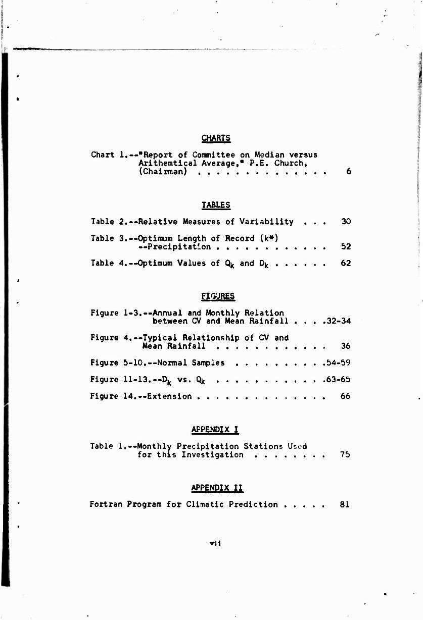
TABLE OF CONTENTS

Abstract ill

I. INTRODUCTION

1.1 Limitation of Study 1.2 Use of Mean and Median 1.3 Early Studies 1.4 Recent Studies 1.5 The Mean as a Poor Estimate of

Central Tendency 1.6 Normals

II. CLIMATIC NORMALS

1 2 3 5

7 9

11

2.1 Data and Study Area 2.2 Procedures 2.3 Skewness 2.4 Analysis of Maps 2.5 Conversion of Existing Maps

III. MEASURES OF DISPERSION

IV. CLIMATIC PREDICTION

4.1 Normals 4.2 Procedures 4.3 Random Numbers 4.4 Analysis

V. CONCLUSIONS

References Appendix I Appendix II

11 13 15 1 19

27

3.1 Absolute vs. Relative Measures of Variability 27

3.2 Absolute Measures of Variability 27 3.3 Relative Measures of Variability 28 3.4 Variability as Related to Rainfall Amounts 31 3.5 Variability Maps 37 3.6 A Note on the Coefficient of Variation 39

49

49 49 51 53

67

71 75 81

MAPS

Map 1.—Station Locations 10

Map 2-3.—Percent of Years with Haintaii exceeding Mean

Map 2 - January 12 Map 3 - April 14 Map 4 - July 16 Map 5 - October 18

Map 6-10.—Ratio of Median to Mean (Percent). . .

Map 6 - January 20 Map 7 - April 21 Map 8 - July 22 Map 9 - October 23 Map 10 - Average of 12 Monthly Values 24

Map 11.--Coefficient of Variation of Annual Precipitation in Percent 38

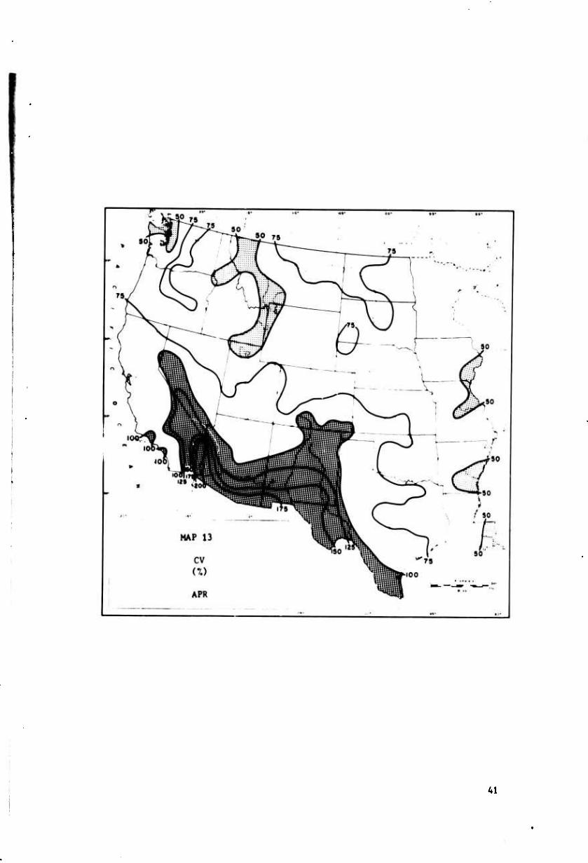
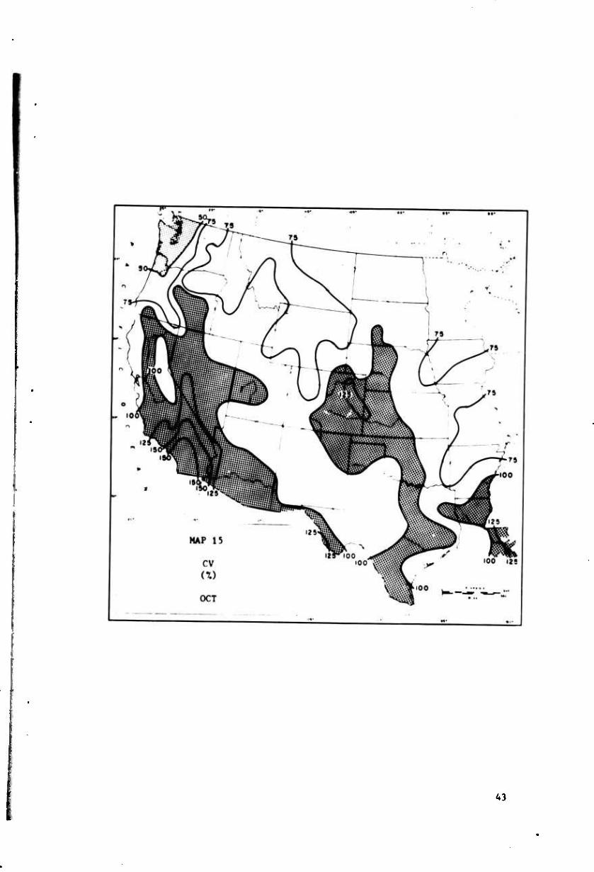
Map 12-15.—Coefficient of Variation

Map 12 - January 40 Map 13 - April 41 Map 14 - July 42 Map 15 - October 43

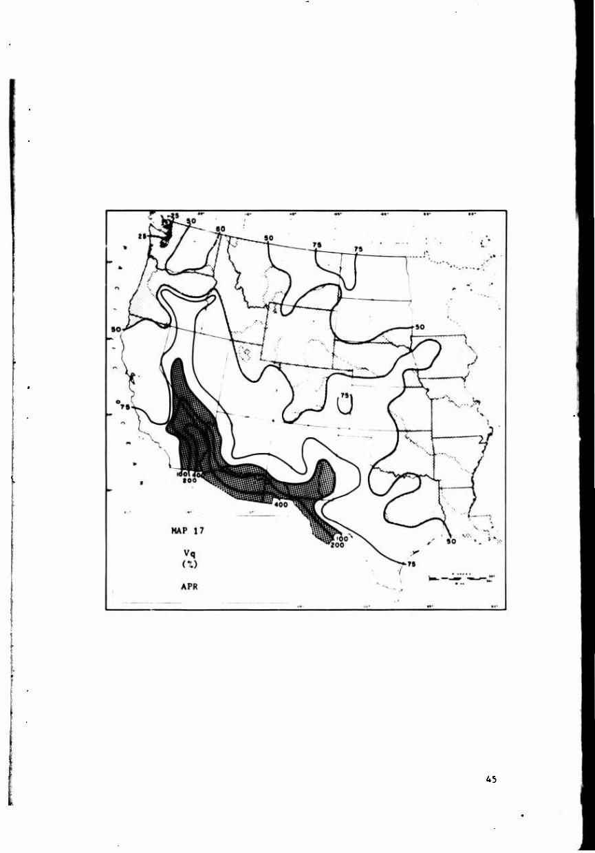
Map 16-19.—Relative Variability

Map 16 - January 44 Map 17 - April 45 Map 18 - July 46 Map 19 - October 47

Map 20.—Station Location and Years of Record . . 60

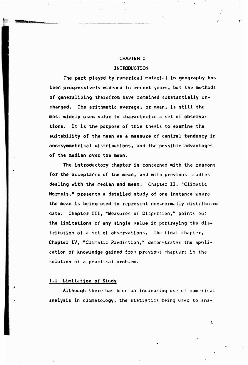
CHARTS

Chart 1.—"Report of Committee on Median versus Arithemtical Average," P.E. Church, (Chairman) 6

TABLES

Table 2.—Relative Measures of Variability ... 30

Table 3.--Optimum Length of Record (k*) —Precipitation 52

Table 4.--Optimum Values of Q^ and D^ 62

FIGURES

Figure 1-3.—Annual and Monthly Relation between CV and Mean Rainfall . . . .32-34

Figure 4.—Typical Relationship of CV and Mean Rainfall 36

Figure 5-10.—Normal Samples 54-59

Figure 11-13.—Dk vs. Qk 63-65

Figure 14.—Extension 66

APPENDIX I

Table 1.—Monthly Precipitation Stations Used for this Investigation 75

APPENDIX II

Fortran Program for Climatic Prediction 81

vli

n:

»t

BLANK PAGE

( * i

m.

CHAPTER I

INTRODUCTION

The part played by numerical material in geography has

been progressively widened in recent years, but the methods

of generalizing therefrom have remained substantially un-

changed. The arithmetic average, or mean, is still the

most widely used value to characterize a set of observa-

tions. It is the purpose of this thesis to examine the

suitability of the mean as a measure of central tendency in

non•symmetrical distributions, and the possible advantages

of the median over the mean.

The introductory chapter is concerned with the reasons

for the acceptance of the mean, and with previous studies

dealing with the median and mean. Chapter II, "Climatic

Normals," presents a detailed study of one instance where

the mean is being used to represent non-normaiiy distributed

data. Chapter III, "Measures of Dispersion," points out

the limitations of any single value in portraying the dis-

tribution of a set of observations. The final chapter.

Chapter IV, "Climatic Prediction," demonstrates the apnli-

cation of knowledge gained fron previous chapters in the

solution of a practical problem.

1.1 Limitation of Study

Although there has been an increasing uso of numerical

analysis in climatology, the statistics being used to ana-

lyze the masses of data have gone unchanged. The statistics

presently in use were developed for use with normal or near

normal samples. Chief among these are the two most commonly

used statistics, the mean and the standard deviation.

Unfortunately, most climatic variables have distribu-

tions other than normal. Singly or doubly bounded variables

have skewed distributions markedly different from the sym-

metry of the normal distribution (Section 2.5). Precipita-

tion, wind speed, insolation, and visibility are a few of

the climatic variables for which the majority of observa-

tions occur at the upper and/or lower limits of their dis-

tributions. In such skewed distributions the mean and stan-

dard deviation do not have all the useful properties as in

the normal distribution. Perhaps the median, and measures

of dispersion about it, may be more useful.

Although the discussion will be limited to the use of

the mean and median in summarizing precipitation data, the

results should be equally valid for other non-negative vari-

ables having substantial frequencies near the lower bound,

and thus having similarly skewed frequency distributions.

Wind speed, income, and agricultural, industrial, or mineral

production by counties, are good examples of such variables.

1.2 Use of Mean and Median

The arithmetic mean is often declared to be the b^at

estimate of central tendency, and hence is the value most

generally used to characterize entire sets of observations.

In a symmetrical distribution, such as the normal, the mean

is also the median or 50% probability value. Thus many

people implicitly regard any mean as having a 50% probabil-

ity level of exceedance. Unfortunately, in skewed distri-

butions, which are more common for geographic data, the

mean is not the median, and only the median has a 50% pro-

bability level of occurrence.

The greater the ekewness of the distribution, the

poorer the mean becomes as an estimate of the middle value,

the median. While the mean may be easier to work with in

many instances, the median or 50% probability value is most

often desired and should be used whenever possible to avoid

any misconceptions regarding frequency of occurrence. In

many applications the mean has been uced, and is continuing

to be used, largely as an approximation of the median.

1.3 Early Studies

The unsuitability of the mean a a measure of central

tendency in climatologicai research hac long been realized,

but it was not until 1933 that a serious attempt was n.:de

to replace the mean with the median to summarize a "varied

me.eorological record." It was in thi£ year that the Bri-

tish geographer, Percy Robert Crowe, introduced the use of

the median and quortile deviation (half the difference bet-

ween the upper and lower quartiles) in a ^tudy cf European

rainfall entitled "Analysis of Rainfall Probability." This

study created much interest and its influence can be seen in

several succeeding studies. The most notable of these is a

study of Indian rainfalls by Matthews (1936). The median

and quartile deviation were again used by Crowe (1936) to

study the rainfall regime of the Western Plains of the

United States, and also by Lackey (1937) in constructing

annual-variability .naps of the Great Plains. Earlier stud-

ies by Lackey (1935, 1936) also show the influence of Crowe.

Other researchers not influenced by Crowe were also

coming to the conclusion that the mean should be replaced

by the median when dealing with a highly variable distri-

bution. Gisborne (1935) used monthly precipitation records

of Spokane, Washington to show that the mean is a poor

value to use as a "climatic normal." He found that the

mean was never reached or exceeded more than 46^ of the

time in any month and that in June the mean occurred only

26?^ of the time. If the mean were used as the "normal,"

74 years out of 100 had below normal precipitation in June.

A similar study was undertaken by Mindiing (1940) using 60

years of monthly precipitation records for each of 14 sta-

tions distributed throughout the United States. His con-

clusions were the same as Gisborne's: the mean is an unsat-

isfactory value to use as a "normal," and that the median

would be a better value to use.

This interest in the proper statistic for use in

representing a non-symmetrical distribution, first seen in

m

I

the studies by Crowe, reached a peak June 20-21, 1940. At

this time a resolution recommending that "the expression of

normals of precipitation in future Hydrologie studies be

defined by the median instead of the arithmetical average"

was presented to the Section of Hydrology of the American

Geophysical Union, meeting jointly with the Western Inter-

state Snow-Survey Conference in Seattle. A committee headed

by P.E. Church (1941) had weighed the advantages and dis-

advantages of each (Chart I) and concluded that "in the

future, at least for Hydrologie studies, the expression of

normals of precipitation be defined by the median,"

Unfortunately the recommendations of this committee

were lost with the on-coming of World War II, as was the

interest stimulated by Crowe and others, and the mean con-

tinues to be used in Hydrologie and climatological studies.

1.4 Recent Studies

Very little discussion of this topic has appeared

since 1941. Landsberg (1947), declaring that the mean does

not represent the usual condition even for monthly tempera-

tures, condemned the use of the term "normal" for the arith-

metic mean. In a study of rainfall on Oahu, Hawaii, Lands-

berg continued, saying that:

The median is the statistic that preserves one 6f the most important properties of a "nor- mal." It represents the center of the distribu- tion and half of the observations are higher, the other half lower than this value. (1951, p. 9)

JUART 1

IM TMHUCTIO». UiniOM OVMTSICAL IMIOM

MNIIT or oomimt on moim vow» MITMRIQU. Avmoc I r. I. Ckurc» (CMlrau). Wtmrt L. M«IU. and ■. P.

la UM iMt MHlM or tkt Mttlnts «f UM SMttM of lydrclHr •! tM AMFIMB OM|ftr«tMl «UM im SMttl« im JMM. 1940, t rtMlutlMi ntcMMMttnt ttet aUt upnmltm •( Mrasls «t pmtptUUM la fkum feydrvugic lUttM M «atlM« ky UM M41M imtmt «f UM arttaMUMl •*•!«••* MS prMMttd. It «M »»«4. HCMM. MM pMMd UMt U» NMllltlMI M rtr«mM U t •MBtttM Mpalata« ky OMirau J. C. SU*«M. CMMOSH of P. I. OMrst (ClMlrau). Mnr« L. Mils. «M 1. P. »mumm, (SM p. 106S. mm. »mr. OMpiura. uaita. If40.|

TIM CMBlttM UM MlghM bou UM advaaugaa aiM «iMdvaaUfM tt tut aMlta «nd U« ■riUMtteal awwgi HM la a* Mil« ay—raaa «TIUBMU. bet» favaraklt «nd «afavaraal«. aw-t

UMT« art aaaaraaa mi« «f Mpraaalat u* Matral tiaiiaip •( a atrlaa at tlMM. (a) arltaaatUal avarag«, (a) (•«attrle aaaa. («) fearwatc ana. «) mlp,** arlttn(lc*i

(a) aada. (t) aaataa. wt (■) truaiaay-aiatrtaatlaaa. UM naalatlaa «alia« far a itlaa at tat aaa at aMitta la prataraaea u UM arlUHMtlaal •«««•••

itacaa and advtataiaa at UM aadlan vwaua tka arltfeaatlaal avaraga ara llatad fealaat

MiüTMmtt ii ttt mam CD Tka aadlan. aa UM MUM at tipraMlag UM MIMI. la Mt «laara ut rigva Mica am

bt raprtaMUtlva at Ua caatral twdMay tar all purpaatt. Par etrUla pirpaMa UM arlUMtlaal avaraga la aara aMtal.

(I) A larga aMMt at Mrk alll 6a ratulrad U racaaputa tM ««at aaaMt at MU M raeard aaa avallMla. Tfela aarfc aMld tall Urtaljr on tka yaatkar Buraau «klek Ma aMaaad Ua VMtar part at Ua daU mm la Ma. TM utatkar MTMU data Mt ka«a MftUlwt aMlaUMa U raaaapat« Uta Mdf at daU at praaaat.

(I) Caaparatlvalp tM pMpla eutaida ua Mtkaaatleal and anclaaariat prataMlaa «MarataM Ua uact aaanlac at Ua MdlM akareta Marly avaryana uMarataMa Ma ua arlUMtlMl a<araca la eaapatad. It Ua aMlan Ma Mad It Mvld ka nacMaary ta iMtniet tMM «alag Ua daU M u ua aaMlag at Ua aMlaa.

(4) MM uara i» M HtaMad ikiMar at aManratloM, Ua arraniaaMt at Ua daU U Mtar- alM Ua BMIM la tadlaua and alttamb M eaapaUtlan ta aacMaary U dataralaa Ula flgara Uara la M aacaiM aa ua aartat Mtu alll aMa Ua aacaaaary arran««aant. It la a alapla aM 9«lck pntaM u aaapwta Ua arltkMtlMl avaraga baewaa Mdtag aaUliMa ara aUaat Mtvaraally awllakta.

(6) Tka aaa at Ua aanUly aadlaM far a yaar Maj Mt MMI Ua aaaaal MdlM. MaraM Ua iM at Ua aMUly arltMatlMl wtratia MMU Ua annual ariuwatieal avaraga. TM aiaiMl aadlM aMld Mm ta ba caapatM frM Ua BMBMI aaewnta.

(•) Mara Mra uan Mit Ua Miuraa ta a aarlaa ara Mra. Ua aadlM aMld aanvay Ua la- praMtan Uat Uara aM a lack af a aaaaurMla quantity.

at tM MdlM (1) Tka BMIM. Mlla Mt alaaya ua figara Mica «111 M raprMMUtlva at Ua caatral

taadaney far all pwrpacat. la auparlar U tka arltanatlcal avaragWln auy caaM. (t) Tka BMIM CM M dataraiaad by a alapla arrangaaMt at Ua tarltt at MaartratlaM aad

M ecapaUtlM la naeaaaary. Ukara aCdlng Mcklnaa ara .->at aaallMla. Ua MtaralMtlan at ua avaraga ta tar Mra tadloua tkan tka aadlM.

(3) TM MdlM ta Maftwud by Ua abMraally lart- ar aMtl valaaa af a aarlaa at M- aarvattaM. la Ua CM* af praeipiuttan Ua abnorMl valMa ara alaaya la aacaaa at MU Ua aadlM aM Ua arlUMtlcal avaragaa bacMM af ua llatttng valu* af »tro. TM arlUMtlaal avaraga la *atrangly lafluaMM by aitraM vartanta ta a aarlM of «aluM.*

(4) la Ua aarlM af eMarvatlana. If uara la a ffMtl» autivinf «alM. altkar raal ar U* raMlt at M arrar. Ua MdlM «ill b* laM affactad tMn ua art' MUMI avaraga.

(6) Mgatlva daparturac at praetplUtlM ara at graatar fraquancy 'IM plM daparUrM aMa tM arlUMtlMl avaraga la MM u Ua aaaaara at Ua central taMency. Tkla aMld Mt M tna MM ua BMIM la MplayM.

(•) TMae Ma BMU aaka Mtlva Ma af Ua aMlan aa tka Mraal ara Mlnly kpdralagtaU. aagtaaara. Mtaaralaglau. au.. BM BMU Mt Mve u M iMtracttd M ta Ua aaaal^ at MdlM. TMM aM M Mt kaM nMt Ua aard aadlM partraya CMld learn Uat M readily aa Ua aaataat at arlUMtlaal avaraga. aaraal. ar aaM. On pMUMM Mta a Mtlnltlon af BMIM caald M laaarud.

m^

In the study of the measurement of water content of a

snow course, Court (1958) found that a water equivalent

figure sufficiently accurate for the prccticai use to be

made of it can be obtained from the median of a small num-

ber of snow course points. He indicates that the combina-

tion of a larger number of snow water content measurements

into ö single mean is Ma gross waste of information from

the statistician's standpoint."

More recently Joos (1964), after a study of the vari-

ability of weekly rainfall, suggested that "a more meanino-

fnl 'normal' for weekly precipitation might be based on the

b0% value rather than on a long term mean," Kangieser

(1966) finds that in some parts of Arizona only one year in

ten has monthly precipitation as great as the mean value.

And Bennett (1967) shows the median to be a better statis-

tic than the mean for the study of insolation which, un-

like precipitation, has a distribution in which many obser-

vations occur near the upper bound.

1.5 The Mean as a Poor Estimate of Central T ndtncy

The mean is too strongly influenced by the extremes in

a series of values. Ten months with values one unit below

the mean are required to neutralize the effect of one month

with a value ten units above the mean. In the case of cli-

mate, it is the time period during which people have to

live and work, the month of the year, that is significant.

The frequency of departures from the normal is important,

but the actual extent of departure of each instance is

secondary.

Yet, it is the mean which is stated in answer to a

question concerning the amount of rainfall a place receives.

At the present time, maps of climatic normals are based on

the arithmetic mean such as those which appear in The Na-

tional Atlas of the United States, published in 1964. The

supposed purpose of these •normal total precipitation"

maps is to give the user an idea of the most likely amount

of precipitation to be received at a particular place.

Since the arithmetic mean can satisfy the concept of normal

only when the data are symmetrically distributed, these

"normal total precipitation* maps are deceptive especially

in drier areas of this country.

It would seem that the median would be a much more

logical measure of central tendency. Since it is the mid-

dle value, it is easily ascertained when the figures are

arranged in ascending or descending order of magnitude and

can thus be located by a process no more complicated than

simple inspection or, at most, by plotting the values con-

cerned on some form of linear graph. With the use of the

high speed computers, even large amounts of data pose no

problem in the finding of the median. Its reality consists

of the fact that, since half of the records exceed it and

half of them are less, it represents the usual or typical

value. It is quite indeperdent of a few very exceptional

values, since each value has an equal pull, whatever its

size. Because of this, the median is less sensitive to

errors which might be present in the data being examined.

1.6 Normals

At the present, one of the primary methods used to

portray climatic data is through the use of a 'climatic

normal.' Climatic normals supposedly describe the climate

of a place or region and are often used to estimate future

climatic conditions. They are calculated by averaging

climatic events over a number of years, usually 30. Al-

though some objections have been voiced against this method

of determining the normal, it is accepted as being the best

possible method by the majority of the people.

As pointed out by Gisborne in 1935, the concept of

normal is well established in both the technical and the

lay mind as that which is common, natural, ordinary, regu-

lar, typical, and usual. It must be determined Just how

well the mean satisfies this definition.

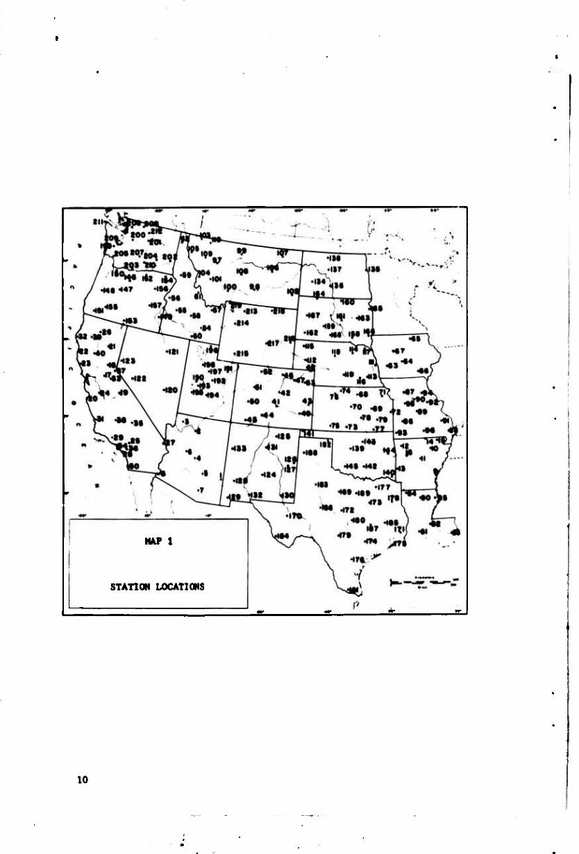
NAP 1

STATION LOCATIONS

10

CHAPTER II

CLIMATIC NORMALS

2.1 Data and Study Area

Used in this study are monthly precipitation values at

219 stations in the United States, all west of the Missis-

sippi River (Map 1). Data were taken from publications of

the United States Weather Bureau, supplemented by data pub-

lished by various states. Stations were selected to insure

homogeneous data: no significant change in station posi-

tion, elevation, or environment during the observation

period. Although some stations had precipitation records

for 110 years of continuous observations, only data from

the period 1931 to 1960 were used. Thus all analyses and

maps in this report are comparable, and are for the period

specified by the World Mtteorological Organization and used

by the United States Weather Bureau to determine climatic

normals.

Table 1 (Appendix 1) is a list of the monthly preci-

pitation stations used in this study. The 219 stations

represent an average density of one station for every 9,789

square miles. While this fails short of the one station

per 1,029 square miles coverage for rainfall by the Nation-

al Atlas of the United States, it compares' favorably with

the density of stations of the Local Climatological Data

published by the United States Department oi iJommerce Wea-

11

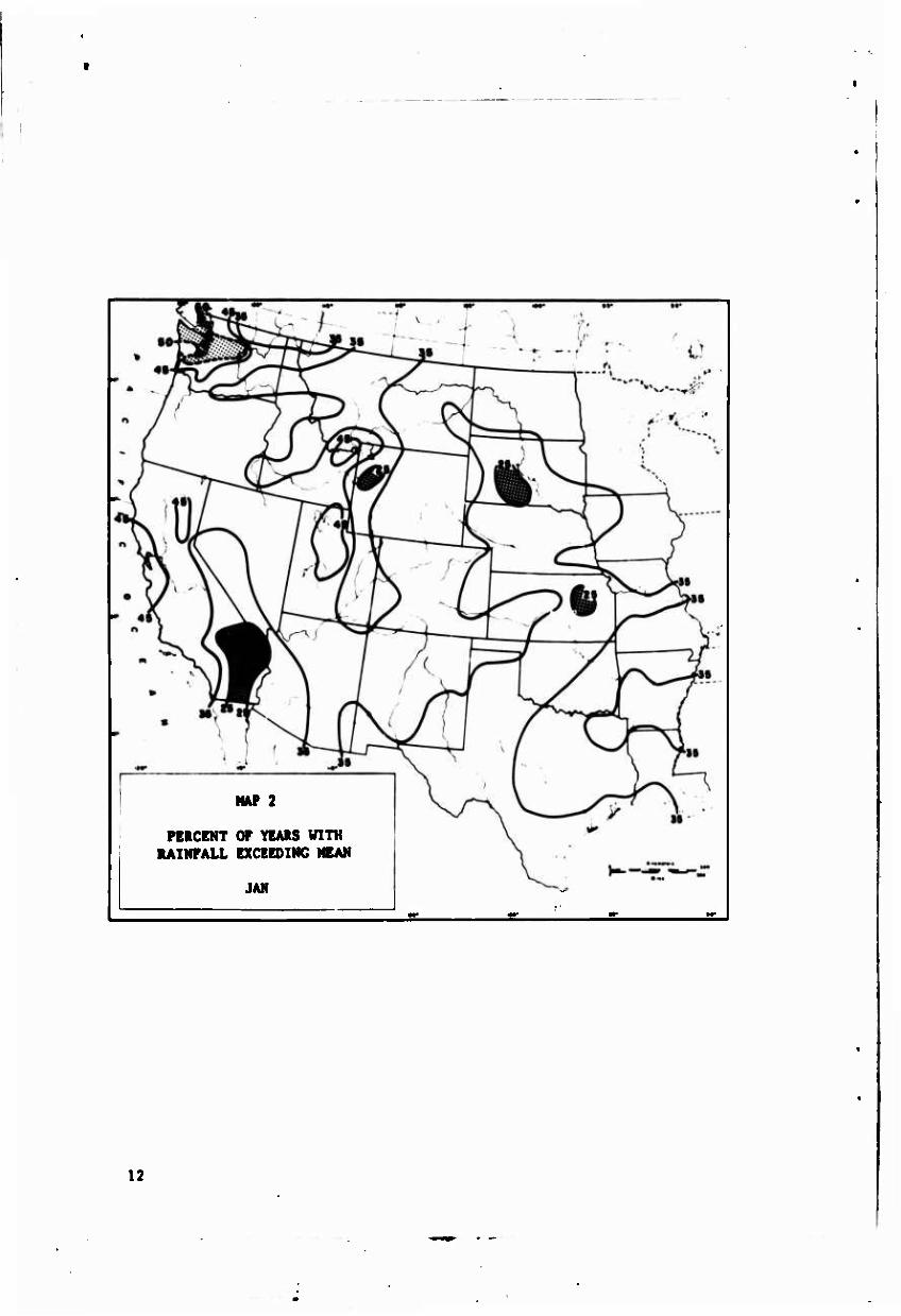
NAP 2

PERCENT OP YEARS WITH RAINPALL EXCEEDING MEAN

JAN

12

ther Bureau (approximately one station per 10,500 square

miles). Stations are listed by their U.S. Weather Bureau

identification number, with name, coordinates, and number

of years of continuous record. For convenience in compu-

tation and mapping, stations are also numbered serially

1 to 219.

Due to the excessive time and work involved in mapping

the results of all months, only the mid-season months of

January, April, July and October are included in this study,

The use of these months should bring out any seasonal vari-

ations that may exist, and should be a large enough sample

to work with. It is important to work with more than one

or two months since the possibility does exist that they

may not be representative of the majority of months. Such

an error was made by McClean (1956) in assuming that con-

clusions reached for one month would apply to all months.

McClean's contention that the period 1881-1915 is a poor

one to use as the standard for reference to British rain-

fall was disproved by Giasspoole (1956).

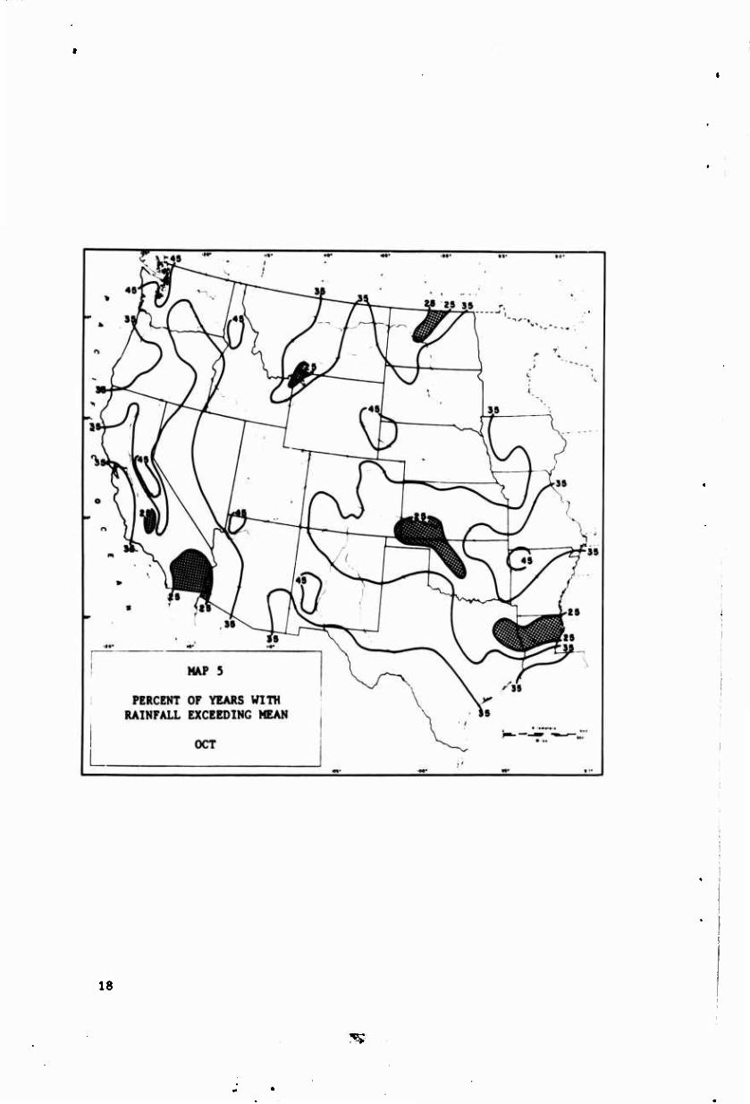
2.2 Procedure

If the limatic normal were a representative value, it

would be expected to be reached in half of the years of

record. The percentages of the years (1931-1960) in which

the "normal" value was reached or exceeded were calculated

and are shown on Map 2-5. These maps snow that the mean

13

MAP 3

PERCENT OF YEARS WITH RAINFALL EXCEEDING MEAN

14

fails to represent the central value of the distribution

from which it is derived, especially for the Southwestern

portion of the country. The inadequacy of the mean as an

expression of the "normal" for monthly precipitation is

shown.

?..3 Skewness

As stated in the introduction, in a ncrrr^l distribu-

tion, or any other symmetrical distribution, the mean is

equal to the median and under such circumstances the mean

is a perfectly valid value to use. But when the distribu-

tion is skewed (asymmetrical), the mean is much less repre-

sentative. A distribution is symmetrical when the median

•quals the mean; positively skewed when the mean is larger

than the median; and, negatively skewed when the mean is

smaller than the median.

There are several ways for measuring skewness. One

of these is the "Pearsonian coefficient of skewness" given

by the formula

3(m3an - median)/standard deviation

Another measure, <s (alpha-three), is defined in terms of

the second and third moments, n^ and 1113, about the m^an

as

*. • */(•*•)*

In this study a simple measure of skewness is given by the

percentage occurrence of the mean as portrayed in Maps 2-5.

IS

MAP 4

PERCENT OF YEARS WITH RAINFALL EXCEEDING MEAN

JUL

16

The further the mean departs from the 50^ probability value,

the greater the skewness and the greater the advantage in

using the median to best represent what is expected to

happen again.

2.4 Analysis of Maps

Before discussing the maps any further, it should be

pointed out that isolines are only as good as the data from

which they are derived. The patterns shown on the maps in

this study are necessarily general due to the number of

stations used. If further data points were available, pat-

terns would undoubtedly be changed. But for the purpose of

the present study the number of stations is adequate. If

further detail is desired, studies of individual states

should be made, such as that of Arizona by Kangieser (1966).

It would have been of interest to compare his maps with the

ones in this study, but unfortunately they are of different

months.

All maps show low values to occur with regularity in

the Southwest, while high values occur in the Northwest.

The mean is reached in as many as 5C$ of the years only

for January in the northwestern section of Washington. If

the mean were a good value to use as a climatic "normal,"

it should have been reached in half the years in all parts

of the countiy. But it is reached in less than a quarter

of the years in many areas of the country, and in fewer

17

18

than one year in ten for the Central Valley of California

in July.

Seasonal variation in the occurrence of the mean can

best be seen in central California. Here the values range

from less than 10^ in July to over 455^ in January.

For all months values from 35^ to 455^ are most common.

There can be seen no general longitudinal or latitudinal

gradation of values, and the only consistencies are the low

values of the southern California desert and the high

values of northwestern Washington.

2.5 Conversion of Existing Maps

If a distribution proves to be skewed, the use of the

mean as the most representative value of the distribution

will be misleading. Under such circumstances the median

should be used. However, considerable work went into the

computation of existing means, and it is doubtful that any-

one would be willing to discard these even if their valid-

ity is in doubt. This problem would be solved if a stable

relationship is found to exist between median and mean.

With this aim in mind, the ratio between median monthly

and mean monthly values was computed for each station

(Maps 6-10). If stable, these ratios can be used as cor-

rection factors to convert existing means to medians (see

Appendix) .

19

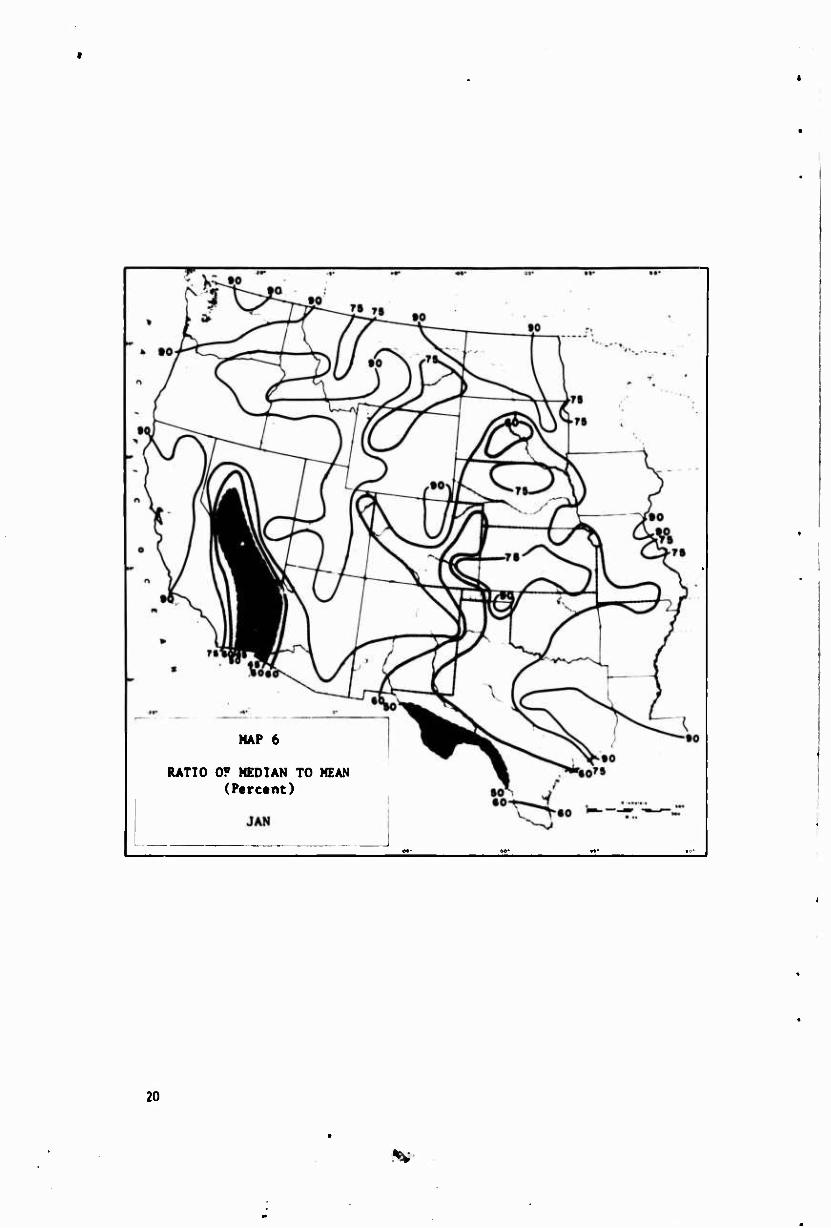
HAP 6

RATIO OF MEDIAN TO MEAN (Percent)

20

**

W«M

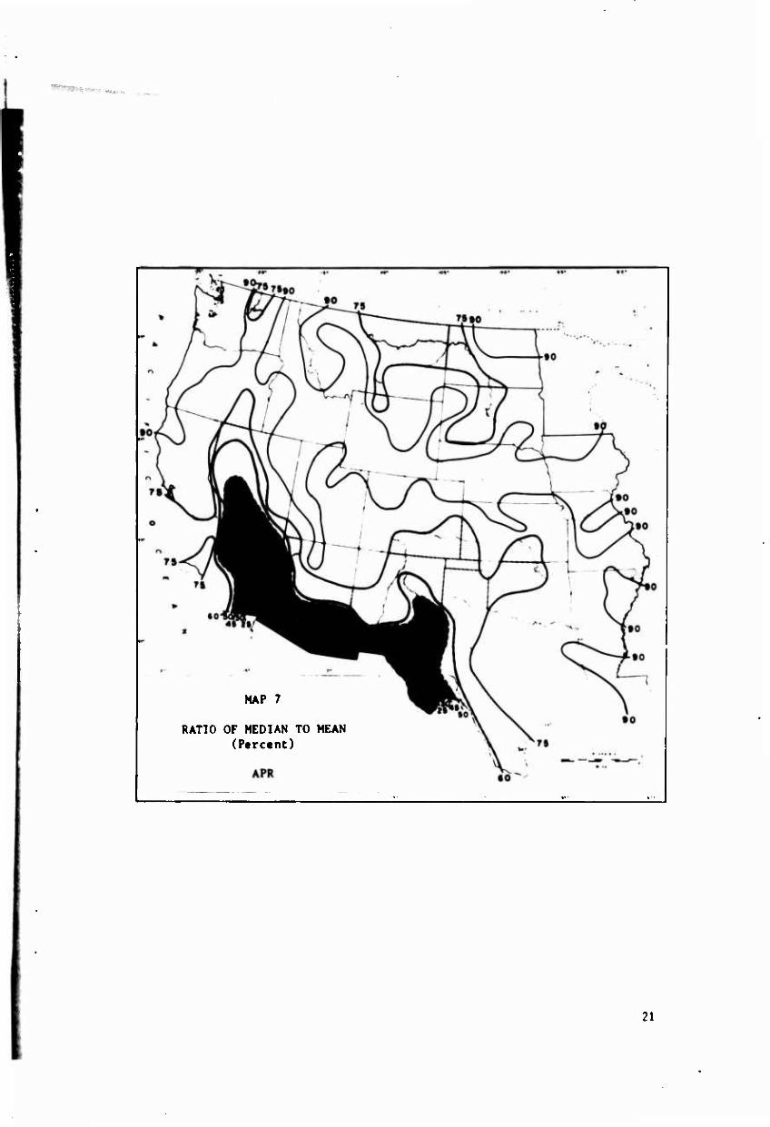
MAP 7

RATIO OF MEDIAN TO MEAN (Percent)

21

MAP 8

RATIO OF MEDIAN TO MEAN (Percent)

22

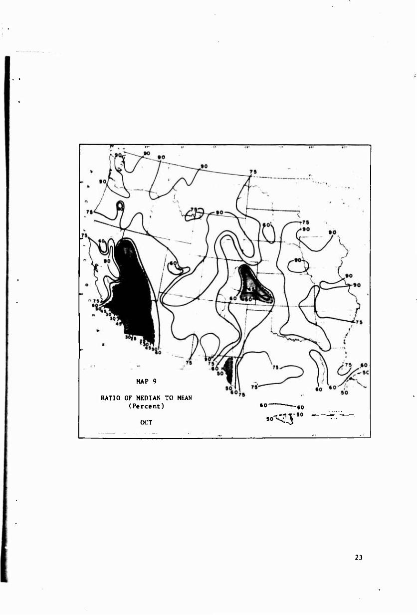
MAP 9

RATIO OF MEDIAN TO MEAN (Percent)

OCT

«o-

30 ^5 • 0

-60 ^-—-

23

MAP 10

RATIO OF MEDIAN TO MEAN (Percent)

AVERAGE OF 12 MONTHLY VALUES

24

The ratios between the median and mean can also be

used as excellent measures of skewness. A ratio smaller

than 1 indicates a positively skewed distribution, while a

ratio larger than 1 indicates a negatively skewed distribu-

tion. The greater the departure from 1, the greater the

degree of skewness.

As would be expected these maps compare favorably with

maps 2-5 with low values occurring in the Southwest and

high values in the Northwest.

Several stations in California had no rain at all

during the 30 years studied for the month of July and had

to be omitted or overlooked in the drawing of isolines,

since in this case the ratios would have been infinite.

25

BLANK PAGE

CHAPTER III

MEASURES OF DISPERSION

3.1 Absolute vs. Relative Measures of Variability

Both the mean and the median have their limitations

in that they are measures of central tendency only. No

single value, however determined, can hope to give a com-

plete descriptive summary. Crowe (1933) pointed out that

we require not only an index of the "normal sequence of

events," but also of the "probable frequency and extent of

variations from the normal."

3.2 Absolute Measures of Variability

The standard deviation is used to estimate the degree

of variability about the mean and defined by the equation

S.d. =

n

irr (xi - x)

1/ 2

where n is the number of values, x. is the individual value,

and x the mean of the n values. But the standard deviation

is not an appropriate t^rm to be u^ed with the median:

while the sum oi the squared deviations is least when com-

puted about the mean, the sum of the absolute deviations is

at a minimum when computed about the median, A measure of

dispersion used to measure variability about the mean or

median is the mean deviation, also known ac the average

27

variability (AV). The mean deviation is defined by the

equation n ,

m.d. = n / Xi - z

where z may be either the mean or median. The semi-inter-

quartile range or quartile deviation q, defined by the equa-

tion

q = (Q3 - Q^/2

where Q^ and Q3 are the first and third quartiles, is used

to estimate the degree of variability about the median.

Other, but poor measures of variability, use only the

highest and lowest recorded values, M and m. The range,

M - m, is often used. Hellman (1909) defined the "ratio of

variation" as the quotient M'm. These measures are not

based on ail observations, and the ratio of variation can-

not be used for desert rainfall: M/m would become infinite

for many stations.

3.3 Relative Measures of Variability

Absolute measures of variability are useful in helping

to understand a particular set of observations, but do not

give a complete picture of the variability. Thus they are

of little value when comparisons between ooservations at

several different localities are desired. This is due to

the fact that variability generally increases as the values

of the observations become larger. Therefore, a map showing

the dispersion of observations about the mean or median at

28

various stations using any of the measures of variability

listed above, would give the same picture as a map of the

means or medians of the observations themselves.

For this reason, relative measures of variability must

be considered in order to derive comparable figures. The

four measures of relative variability corresponding to the

first four measures of variability mentioned above are

given in Table 2.

Of these measures, only CV and Vr have been studied to

any great extent. In studying the relative variability (Vr)

of precipitation, Conrad (1941) found that a very strong

mathematical dependence of the value of Vr on the yearly

sum occurs when these sums are below 1000mm (39.4 inches).

Because of this he concluded that the relative variability

(\/r) cannot be used to compare the variability of precipi-

tation in a locality with a small annual fall with that in

another locality where the precipitation is large.

In a study of all four measures, Longley (1952) tound

the coefficient of variation the most satisfactory measure

for comparing variability of precipitation between dif-

ferent stations. It was found to have small errors through

sampling, in that the values of CV are comparable even when

the mean precipitation values are quite different.

Longley also found that variability tends to be greater

where the precipitation is least, but the relationship was

not close. In a study of precipitation data at 34 stations

29

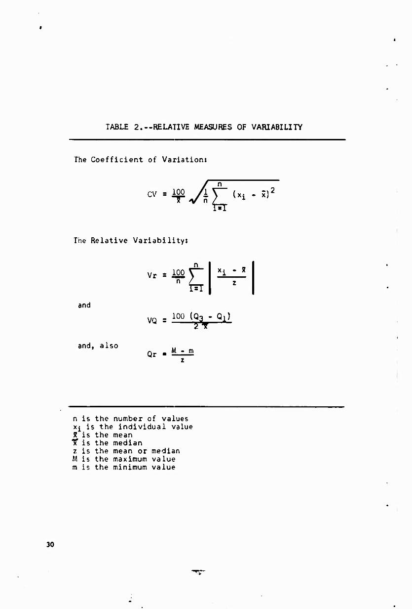
TABLE 2.—RELATIVE MEASURES OF VARIABILITY

The Coefficient of Variation:

CV = 100 ^U7' ü)2

The Relative Variability:

and

n vr = My" x^ - R

VQ -100 (Qy Q''

and, also Qr M - m

n is the number of values x^ is the individual value S is the mean T is the median z is the mean or median M is the maximum value m is the minimum value

30

in British Columbia and Washington, he found the coefficient

of correlation between mean precipitation and the coeffi-

cient of variability to be -0.68 for July, -0.71 for Decem-

ber, and -0.48 for the annual data.

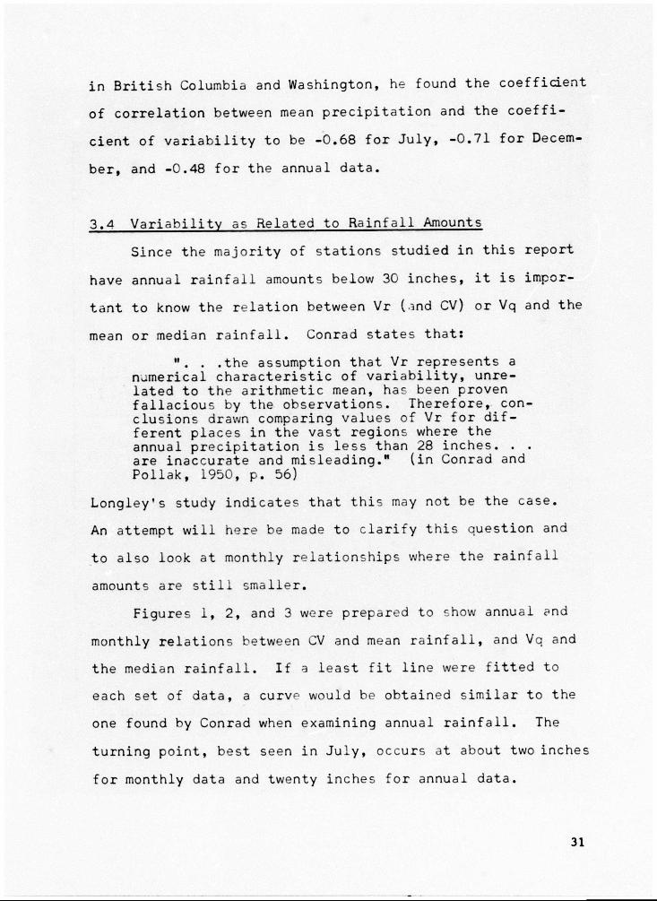
3.4 Variability as Related to Rainfall Amounts

Since the majority of stations studied in this report

have annual rainfall amounts below 30 inches, it is impor-

tant to know the relation between Vr (ind CV) or Vq and the

mean or median rainfall. Conrad states that:

". . .the assumption that Vr represents a numerical characteristic of variability, unre-lated to the arithmetic mean, has been proven fallacious by the observations. Therefore, con-clusions drawn comparing values of Vr for dif-ferent places in the vast regions where the annual precipitation is less than 28 inches. . . are inaccurate and misleading." (in Conrad and Pollak, 1950, p. 56)

Longley's study indicates that this may not be the case.

An attempt will here be made to clarify this question and

to also look at monthly relationships where the rainfall

amounts are still smaller.

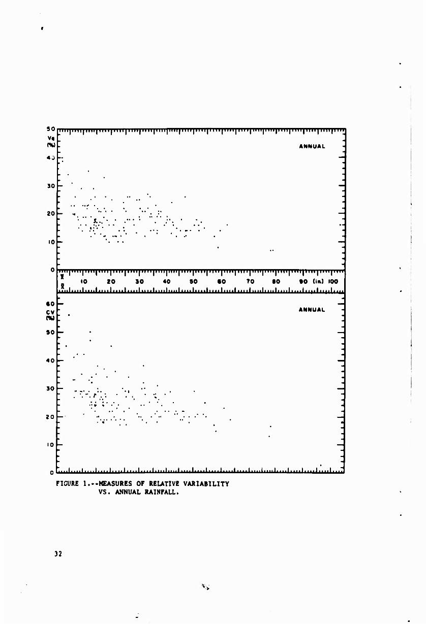
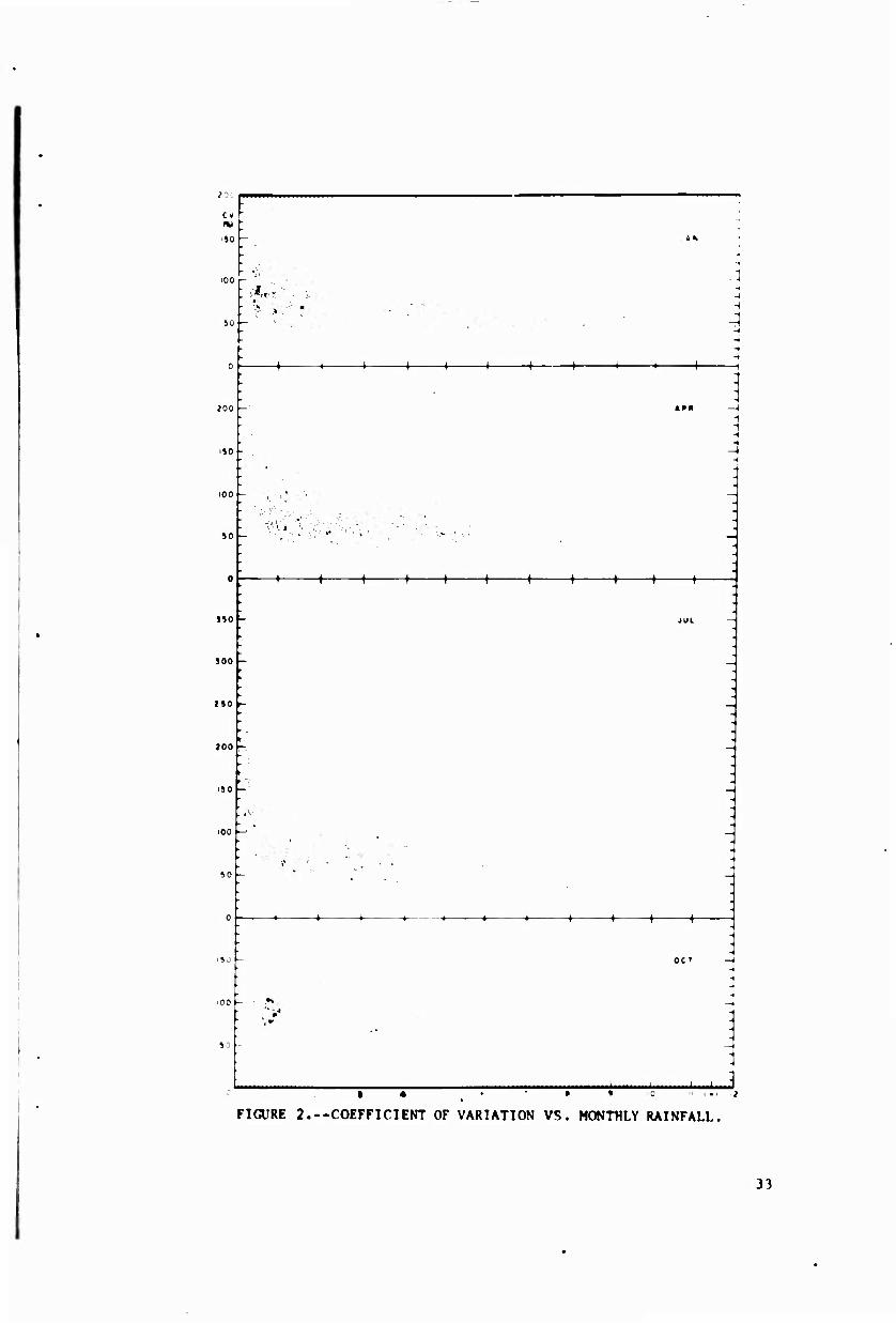
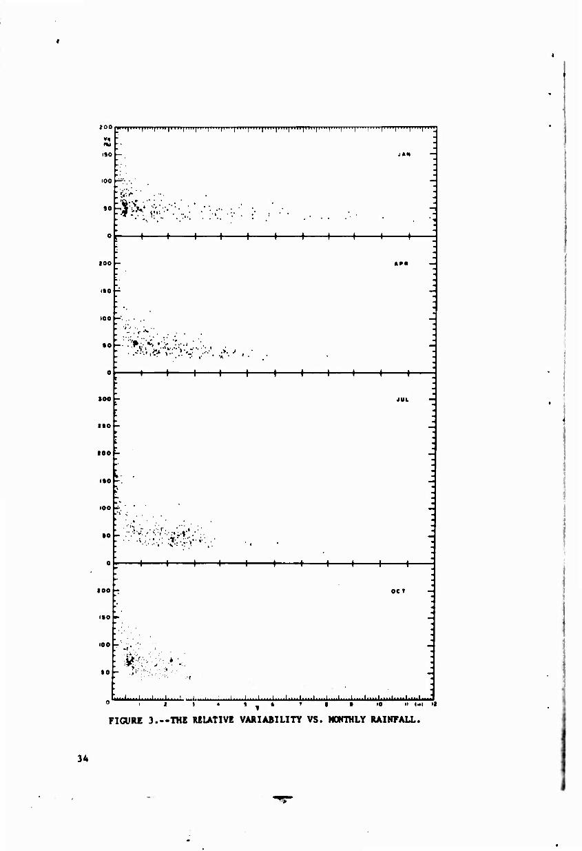
Figures 1, 2, and 3 were prepared to show annual and

monthly relations between CV and mean rainfall, and Vq and

the median rainfall. If a least fit line were fitted to

each set of data, a curve would be obtained similar to the

one found by Conrad when examining annual rainfall. The

turning point, best seen in July, occurs at about two inches

for monthly data and twenty inches for annual data.

31

50

Vq (%)

4J

30

20

10

LMM|iiii|iiiHiiii|im|iiii|im|mi|im|iiii|iiii|iimmniiii|mi|im|im|im|iiinmi|i

ANNUAL

J.. •• •

iMi|iiii|tni|iiii|iiiiiiiii|iiii|iiti|iiiniiiniiinnmiiii|inniiii|iiiniiiniin|iiii|iiinnii 10 20 90 40 SO «0 70 tO tO Umi 100

miliiiilimliiiilmiliHilmilimlmilmiliinlmiliiiilmilimlimlimlimlimlmilm!

•0 cv

50

40

SO

20

10

ANNUAL

t ... • - • • r ♦ * • •

o r....i....i....i.J..i....i....i....i....i....i.i..l....i....i....i....i....i.i.ii....i....i....i....i....

FIGURE 1.--MEASURES OF RELATIVE VARIABILITY VS. ANNUAL RAINFALL.

32

S

^ ■: - C< - m : , iiO

- ■ . .

A #y

■•

IOO : ■4 ■4

so 4 - m

- - - - - -1

0 1 1 1 i i 1 1 1 T -—T—■— ■-t ♦ J " -

- - too — A»« —. • i - i - -I - ■J >so - — *

■ -1 • - - - - IOO — i " i _ ■ • —

■ ; ■' " ■*' ■i '"' ■': i .-,•'. , '

so "

A A

0 1 » i i i t t f I 1 ? f T ,

- - »so JUL

- )00

- -

2SO

ZOO

. ISO

r A- . 100

• • ~

*0 — • -

. o i J, i f f t .

- . -

no oc» —. ■«

-i - <

.00 •v — '■•* - , (F - , » . .

s: - - - ■

FIGURE 2.--COEFFICIENT OF VARIATION VS. MONTHLY RAINFALL.

33

200

tXI

ISO

100

90

i[im[iiiHi iii[iiii[im|iiii[iiiijHii|iiiHHii[iiii[iiii|mi[iiii|i »T'TTTTTtTTJTTTTTTTTTTTTTT

:*<- 'Li.. •►.•*••

H 1 1 1 1 I I h H h

too -

l»0 -

100

• 0

—t 1 1—• 1 1 I i > l I

«»a —

100

1*0

100

ISO

■ 00

• 0

JUL —

i. /ri..- ..• r. ■ ..« .:■

H 1 1 1 I I h—I 1 1 »-

too

1*0

100

«0

OCT -

-'•---'■■■ '■■■■'-■ ' J I — 1 1 — I I 1 — I....I — I 1.... I 1....I....I

FIGURE 3.—THE RELATIVE VARIABILITY VS. MONTHLY RAINFALL.

34

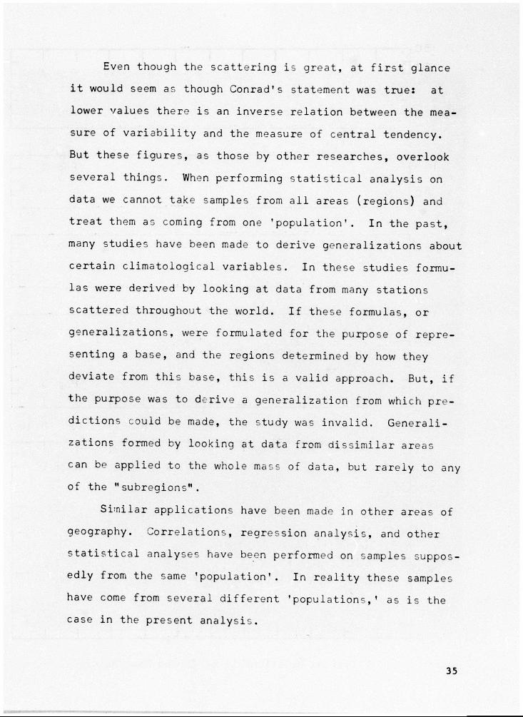
Even though the scattering is great, at first glance

it would seem as though Conrad's statement was true: at

lower values there is an inverse relation between the mea-

sure of variability and the measure of central tendency.

But these figures, as those by other researches, overlook

several things. When performing statistical analysis on

data we cannot take samples from all areas (regions) and

treat them as coming from one 'population'. In the past,

many studies have been made to derive generalizations about

certain climatological variables. In these studies formu-

las were derived by looking at data from many stations

scattered throughout the world. If these formulas, or

generalizations, were formulated for the purpose of repre-

senting a base, and the regions determined by how they

deviate from this base, this is a valid approach. But, if

the purpose was to derive a generalization from which pre-

dictions could be made, the study was invalid. Generali-

zations formed by looking at data from dissimilar areas

can be applied to the whole mass of data, but rarely to any

of the "subregions".

Similar applications have been made in other areas of

geography. Correlations, regression analysis, and other

statistical analyses have been performed on samples suppos-

edly from the same 'population'. In reality these samples

have come from several different 'populations,' as is the

case in the present analysis.

35

150

100 —

100 —

50 —. — •••*.• • •

• .' • • •.

• • • • .

• - •;•.•..••••• •• •

• • • • • —

- Pop. 0 -

" i I I I ■ i i i i i i "

6 ID II (in.) 150 CV (%)

100 1-^

50

Jill i i i i i i i i A ■■ • Pop. A,B.cao -\ ■»•.. — .*:.. —

• •

~:v. '■•• • -

• •

•

•

• • • __ •• • • • • • • ^% • • • . • • •

• • • ; • • .. • •

. • #. .••••. • • . • • • • •» •

-

"iii i i i i 1 1 1 1 "

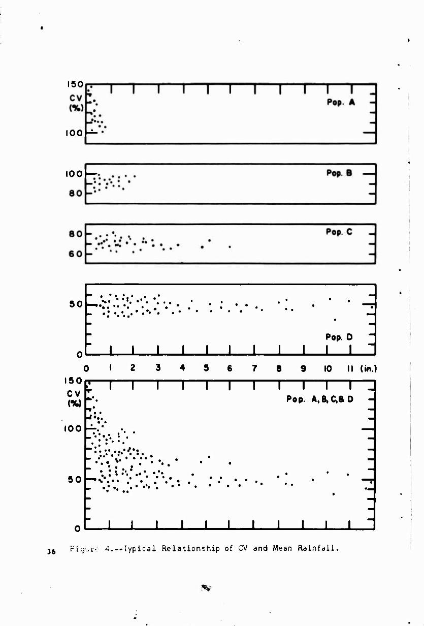
36 Figure 4.--Typical Relationship of CV and Mean Rainfall.

In the majority of previous studies of CV, Vr, and Vq,

data from widely scattered stations in regions with vastly

different rainfall characteristics were treated as coming

from the same population (or region). The results of these

studies supposedly represented the behavior of these mea-

sures of relative variability for all areas. That this is

hardly fact can be seen by looking at the behavior of these

measures separately for several- different areas. Such a

study is presented in Figure 4 where the populations or

subregions are represented by A, B, C, and D. The bottom

graph in Figure 4 shows the typical curve obtained when

data from many different populations are grouped together.

It can be seen that a generalization arrived at by consid-

ering populations A, B, C, and D grouped together would not

necessarily hold true for each individual population. A

large inverse relation between CV and the mean rainfall

occurs only with population A and this is not surprising.

Any measure of relative variability would be expected to

increase rapidly as the average rainfall approaches zero,

since any number divided by zero is infinitely large. Al-

though only CV is discussed in this example, the same rela-

tionships were found for Vr and Vq to varying degrees.

3.5 Variability Maps

While many maps of mean annual and mean monthly preci-

pitation for the United States exist, few maps exist cover-

37

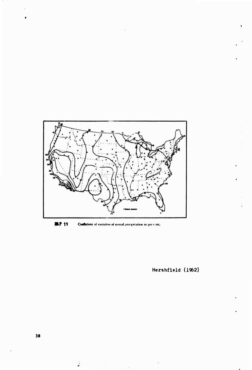
NIP 11 Coefficient «( varialiou ol anmul |iriti|>ii.ili"ii in |«tr «.ill.

Hershfield (1962)

38

ing extended regions which show some measure of dispersion

of the annual or monthly totals around their means. Two

maps were uncovered showing the annual values of the coef-

ficient of variation; the first by Hazen (1916), and the

second by Hershfield (1962) (see Map li) . No maps were

found showing monthly rainfall variability although the

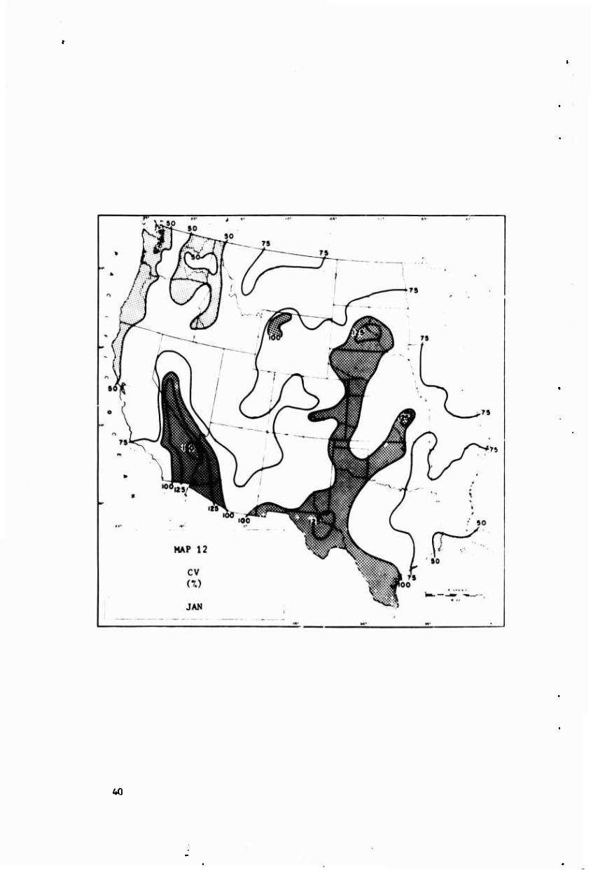
need for such maps was realized by Hershfield. Maps 12-15

showing monthly values of the coefficient of variation were

prepared to partially meet this need and to show the relia-

bility of the mean.

No maps were found of extended regionc snowing the

dispersion of values about the median. While the coeffi-

cient of variation is a suitable term to use in measuring

the dispersion around the mean, a good index of variability

around the median is obtained by • ^pressing the quartiie

deviation as a percentage of the median. Maps 16-19 wert-

prepared using values determined in thic. manner.

3.6 A Note on the Coefficient of Variation

The coefficient of variation (JV) becomes meaningless

in terms of normal probability theory when it become; larger

than 1.00 since the standard deviation oi a norrr.aiiy distri-

buted variable cannot be larger than the mean. But, if CV

i" looked at as a measure of dispersal divided by a measure

of central tendency, without reference to ti.. typ-.- ot dis-

tribution, it becomes very useful.

39

AO

41

42

43

44

45

46

47

Hastings (1965) suggests that CV can be used for

ciimatoiogical and ecological classifications, and as an

indicator of rainfall probability. If seasons are ranked,

the one with the lowest coefficient being 1 and the highest

4; the rank-sequence can be used to delineate regions.

Such a classification reflects accurately tne relative va-

lue of moisture in that it takes into account not only sea-

sonal variability and amount of rainfall, but also the

reliability of the amount.

The coefficient ot variation is also a measure of

skewness. Where CV exceeds 0.5 {t0%) skewing sets in.

When CV exceeds i.OC (100%) non-normality increases rapidly.

48

CHAPTER IV

CLIMATIC PREDICTION

4.1 Normals

In previous chapters the question of what statistic

best represents the 'normal' was investigated. In this

chapter the length of record upon which to base the normal

will be examined.

As mentioned earlier, one of the prime uses of the

normal is as a predictor of future evcnte. At present,

climatic normals are based on 3C yearc of record. Many

studies (as summarized by Court, 1967) show this may not be

the optimum length of record. In the e stuoies, means of

varying lengths of record were used in determining the op-

timum length of record. No attempt hdr y*.-t be^n found to

use the median in relation to this question. In the pre-

sent study, the median o*. varying lengths of record wiix be

used as the predictor of future event"" ana the results com-

pared with those obtained through the us«- of the mean.

4.2 Procedures

One of the most gen^ rally used procedur-j" for deter-

mining the optimum length of record is to calculate the

averages of the squared differences betweon the means of

varying numbers of observations and the values being pre-

dicted. Using the notation adopted by Court {i967) this

49

•xtrapoiation variance, 3 uj«, is computed as

km i ^ v n-k-m+i /

km'

n-k-m+1

ITT

xi+ki-m-l

k-1

k / x,.• 3^ü i+:|J

(1)

where k is the number of antecedent observations from which

a mean (or median) is computed; m is the lag between the k

year period and the value being estimated; and n the number

of observations x^ ordered in time from x, to xn.

In the present stujy this equation was modified to

give Dj^, the average of the absolute differences between

the medians He) of k years and the values being estimated,

as n-k-m+1

(2) Dkm = _1 Y n-k-m-Ti /

[^r 'l+k+m-l - x k,i

where 7^ ^ represents the median of k years beginning with

the observation xi.

Since S^ and D^m are not comparabl» (the first being

an average of squared differences and the second being an

average of absolute differences), a third value, Q. , the

mean prediction error, was calculated as

n-k-m+1

«km--i y ' n-k-m+T /

17T

k-1 x. , , , , ~ 1 V- x :i+k-t-m-l i+j

(3)

As Q, represents tne average of absolute differences bet-

ween the means of k years and the values h ing c-stimated,

it is directly comparable to Du^

50

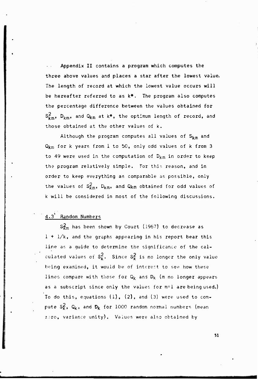
Appendix II contains a program which computes the

three above values and places a star after the lowest value.

The length of record at which the lowest value occurs will

be hereafter referred to as k*. The program also computes

the percentage difference between the values obtained for

^ktn' ^km' ancl ^km at k*, the optimum length of record, and

those obtained at the other values of k.

Although the program computes all values of Sj^ and

Qkm for k years from 1 to 50, only odd values of k from 3

to 49 were used in the computation of Dkm in order to keep

the program relatively simple. For this reason, and in

order to keep everything as comparable as possible, only

the values of S^m, D^, and Qkm obtained for odd values of

k will be considered in most of the following discussions.

4.3 Random Numbers

Sj£m has been shown by Court (1967) to decrease as

1 + 1/k, and the graphs appearing in his report bear this

line as a guide to determine the significance of the cal-

culated values of Sj^. Since S^ is no longer the only value

being examined, it would be of interert to see how these

lines compare with those for Q^ and Dk (m no longer appears

as a subscript since only the values for m=l are being used.)

To do this, equations (1), (2), and (3) were used to com-

pute Sf, Qk, and D^ for 1000 random normal numbers (mean

zr-ro, variance unity). Values were also obtained by

51

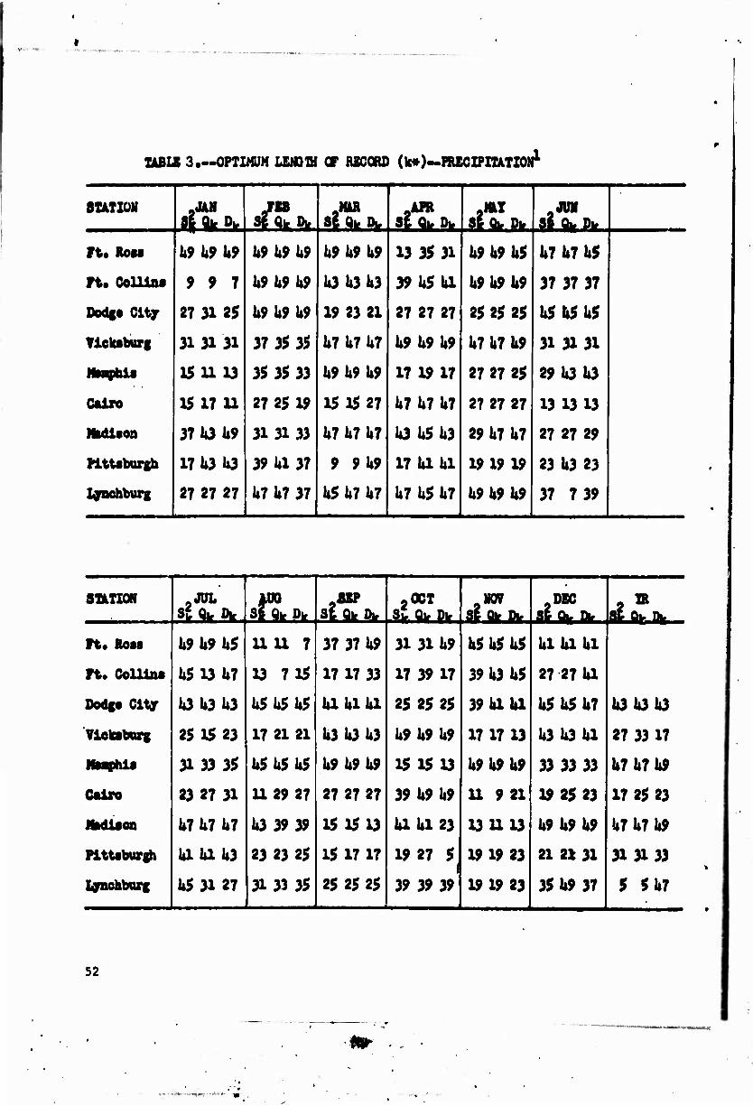
IABLE 3.—OPTIMUM LEMQU GF RECORD (k*)—FRECXPIftTZON1

STATION

Ft« Rotf

Ft» Gellinf

Oodgt City

?lektburg

MMphli

Cairo

Ihdltoa

HtUburgh

Igpaohburg

9<M

U9 h9 k9

9 9 1

27 31 25

31 31 31

151113

15 17 U

37li3U9

17U3U3

27 27 27

HQk ft,

U9 k9 k9

k9k9k9

h9 U9 U9

37 35 35

35 35 33

27 25 19

31 31 33

39 Ul 37

U7 1»7 37

7m

1

1*9 U9 U9

U3b3b3

19 23 21

U7 U7 U7

1*9 1*9 1*9

15 15 27

1*7 1*7 1*7

9 9 1*9

1*5 1*7 1*7

2A»

13 35 31

39 1*5 a

27 27 27

1*9 1*9 1*9

17 19 17

1*7 1*7 1*7

1*3 1*51*3

17 1*11*1

1*7 1*5 1*7

9ÄI St Ql, Dir

1*9 1*9 1*5

1*9 1*9 1*9

25 25 25

1*7 1*7 1*9

27 27 25

27 27 27

29 1*7 1*7

19 19 19

1*9 1*9 1*9

.JUV ?l 9k Plr

1*7 1*7 1*5

37 37 37

1*5 1*51*5

31 3131

29 1*3 1*3

13 13 13

27 27 29

23 1*3 23

37 7 39

sanoN 9JÜL StQwOir sfoLük. St Qlr D.,

2 XT sEokLDk

.DEC douDk -

Ft. Rosa 1*9 1*9 U5 1111 7 37 37 1*9 31 31 1*9 1*51*51*5 Ulla 1*1

Ft. COIUM 1*5 13 1*7 13 715 17 17 33 17 39 17 39 1*3 1*5 27 27 U

Dodgt City 1*3 1*3 1*3 1*51*5 1*5 1*11*1 Ul 25 25 25 39 la 1*1 U5 U5 U7 U3 U3 U3

tiekiburg 25 15 23 17 21 21 1*3 1*3 U3 1*9 1*9 1*9 17 17 13 1*3 1*3 Ul 27 33 17

ÜMphit 3133 35 1*51*51*5 1*9 1*9 1*9 15 15 13 1*91*9 1*9 33 33 33 U7U7U9

Cairo 23 27 31 1129 27 27 27 27 39 1*9 1*9 U 9 21 19 25 23 17 25 23

Jhditoa 1*7 1*7 1*7 1*3 39 39 15 1513 Ul 1*1 23 13 1113 U9U9U9 U7 U7 U9

Plttiburtfi 1*11*11*3 23 23 25 15 17 17 19 27 5 19 19 23 21 21 31 313133

Ijaohborg 1*5 31 27 31 33 35 25 25 25 39 39 39 19 19 23 35 U9 37 5 5U7

52

-*♦.-.-W^,»; .-*i-«-»*

■I

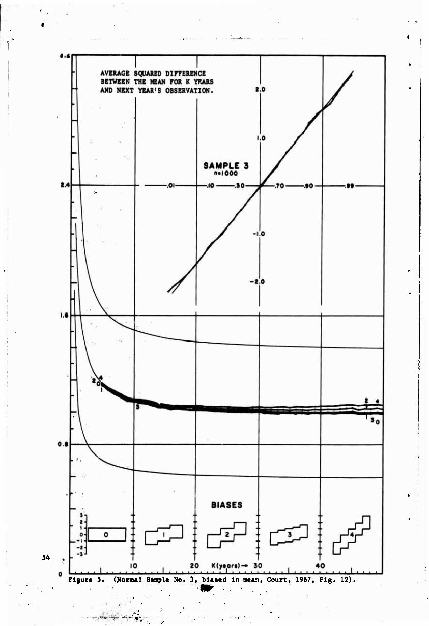
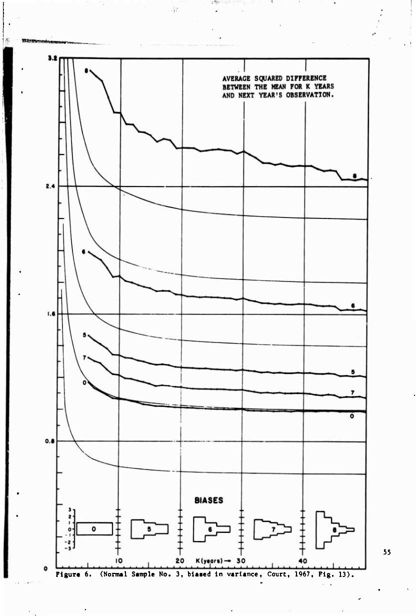
biasing this sample, as in Court's study, in mean and in

variance as depicted on the bottom of Figures 5-10.

The main difference between the three measures is

the rate of change as k becomes larger. Sj~ shows the

greatest amount of variance while Q^ shows the least.

There can be seen no significant difference between Q^ and

Dj^ when values of k are above 15. With biasing, all three

behave in the same manner and a detailed discussion of the

possible significance of this behavior is given in Court's

paper.

4.4 Analysis

For purposes of comparison, the seven stations for

which S^m values have already been determined in Court's

study (1968), along with Fort Collins and Fort Ross were

chosen for study. The latter two stations were included

so that data from drier regions might also be studied. Lo-

cations for these stations along with the number of years

of record are given in Map 20.

In a preliminary study Q^ and D^ were computed for the

above stations and the values of k* listed, along with those

for S^, in Table 3. Examination of this Table shows that

nc method of computation is consistently better than anothei;

and that in the majority of cases, k* values are identical.

I. seems obvious that such an approach is unsatisfactory

for the purpose of determining the advantages of the mean

or median.

53

-A.. -

54

Figur« 5. (Normal Samp 1« No. 3, biased In mean, Court, 1967, Fig. 12).

^..»wifijp''^*' ♦V"

.-

55

Figure 6. (Normal Sample No. 3, biased in variance, Court, 1967, Fig. 13)

FIGURE 7.

56

. . k'ijt^iifttfll'J^, i

-r

0.4

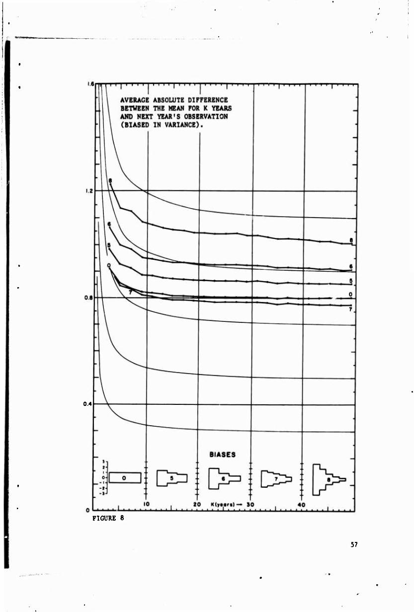
FIGURE 8

57

FIGURE 9.

58

■

.^^-■y^r--^-'^.

i.e n i i i i i i i i i i i i i i i i i i [ i i > i i r i i

AVERAGE ABSOLUTE DIFFERENCE BETWEEN THE MEDIAN OF K YEARS AND NEXT YEAR'S OBSERVATIONS

i i i i | i i TT i i i i l i i r i

FIGURE 10.

59

M i Ü 8 «

O s u w cc

e

J c e a. i (A <

5 Ul

X

H >■ V)

60

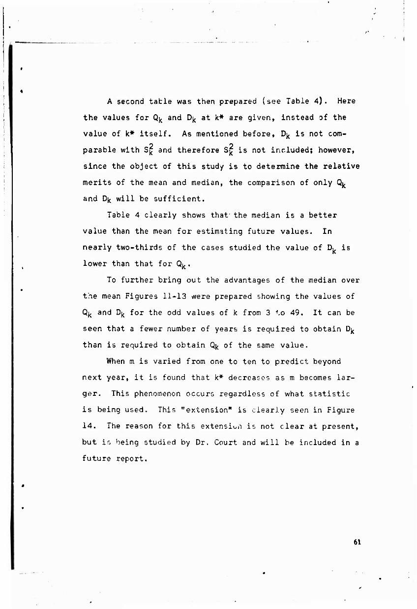
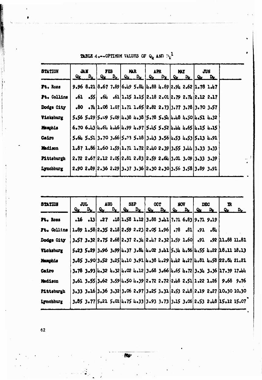
A second table was then prepared (see Table 4). Here

the values for Q^ and D^ at k* are given, instead of the

value of k* itself. As mentioned before, D^ is not com-

parable with Sj^ and therefore Sj^ is not included; however,

since the object of this study is to determine the relative

merits of the mean and median, the comparison of only Q^

and D^ will be sufficient.

Table 4 clearly shows that the median is a better

value than the mean for estimating future values. In

nearly two-thirds of the cases studied the value of Dj^ is

lower than that for Q^.

To further bring out the advantages of the median over

the mean Figures 11-13 were prepared showing the values of

Qj^ and D^ for the odd values of k from 3 to 49. It can be

seen that a fewer number of years is required to obtain D^

than is required to obtain Q^ of the same value.

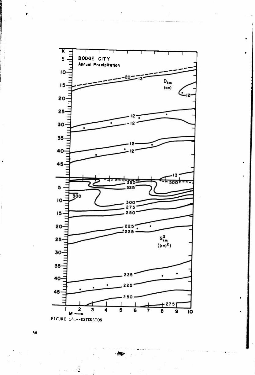
When m is varied from one to ten to predict beyond

next year, it is found that k* decreases as m becomes lar-

ger. This phenomenon occurs regardless of what statistic

is being used. This "extension" is clearly seen in Figure

14. The reason for this extension is not clear at present,

but is being studied by Dr. Court and will be included in a

future report.

61

n.l ÜBLE 4 •—OPTIMUM VALUES OF Qk AND nk. .

STATION

Ft« Rosa

ft. Collins

Dodgs City

Vieksburg

lisa«his

Cairo

Ifedison

Pittsburgh

loraohburg

JAN

9.96 8.21

•61 .55

•60 «ft

5^56 $.29

6.70 6.U3

5.61» $.Sl

1.87 1.86

2.72 2.67

2.90 2.89

FEB

8.67 7.89

.6U .61

1.08 1.07

5.09 5.09

U.6U hM

3.70 3.66

1.60 1.59

2.12 2.Q5

2.36 2.29

MIR 3k. 6.1i9 5.81*

1.15 1.15

1.71 1.65

U.38 U.38

U.99 U.97

5.?3 5.18

1.71 1.72

2.81 2.83

3.37 3.36

APR 9k Dk

U.88 U.89

2.18 2.01

2.82 2.73

5.78 S.SU

5.U5 5.52

3.1i3 3.56

2.U0 2.39

2.59 2.6li

2.30 2.30

nur an Pk

2.9U 2.62

2.79 2.7U

3.77 3.78

luU8 U.50

l*.liU li.65

li.53 li.53

3.55 Uh

3.01 3.09

3.56 3.58

JUN ^k St 1.78 l.li7

2.12 2.17

3.70 3.57

U.51 U.32

U.15 U.15

5.13 lu91

3.33 3.33

303 3.39

3.89 3.91

stktm JUL Qk D^

ATO Qw Dk

SEP OCT Qlr Die

NOT Qw Olr

DEC IR Qlr Dl,

Ft« Ross .16 .13 .27 .18 1.58 1.12 3.88 3.U1 7.71 6.83 9.71 9.19

Ft. Collins 1.89 1.58 2.35 2.16 2.59 2.23 2.05 1.96 .78 .81 .91 .8U

Dodgs City 3.57 3.32 2.75 2.66 2.37 2.3U 2.U7 2.32 1.59 1.60 .91 .92 11.88 U.81

Tieksburg 5.23 5.29 3.96 3.99 U.37 3.8U U.02 3.U1 5.3U U.S6 U.55 U.22 18.1118.13

Jtaspbis 3.85 3.90 3.52 3.25 U.10 3.91 U.38 U.29 U.U2 U.27 U.81 U.58 22.8U 21.21

Cairo 3.78 3.93 U.32 U.32 U.02 U.12 3.68 3.66 14.65 U.72 3.3U 3.36 17.39 17.UU

Nsdison 3.61 3.55 3.62 3.59 U.50 U.39 2.72 2.72 2.1|6 2.51 1.22 1.26 9.68 9.76

Pittsburgh 3.33 3.16 3.36 3.32 3.06 2.97 3.25 3.31 2.53 2.U6 2.19 2.27 10.30 10.30

Ijnchbttrg 3.85 3.77 5.21 5.01 U.75 U.33 3.93 3.73 3.15 3.06 2.53 2.U8 15.12 15.07

62

6.0

(CM)

I I I I I I i

4 8

AVERAGE ABSOLUTE DIFFERENCE BETWEEN THE MEDIAN (A) OR MEAN (B) OF K YEARS AND NEXT YEAR'S OBSERVATION.

i i i i I i i i i i i i i I i i i i i i i i I i i i i ■ i i i I i i i i

DOOOE CITY PHECIWWION

63

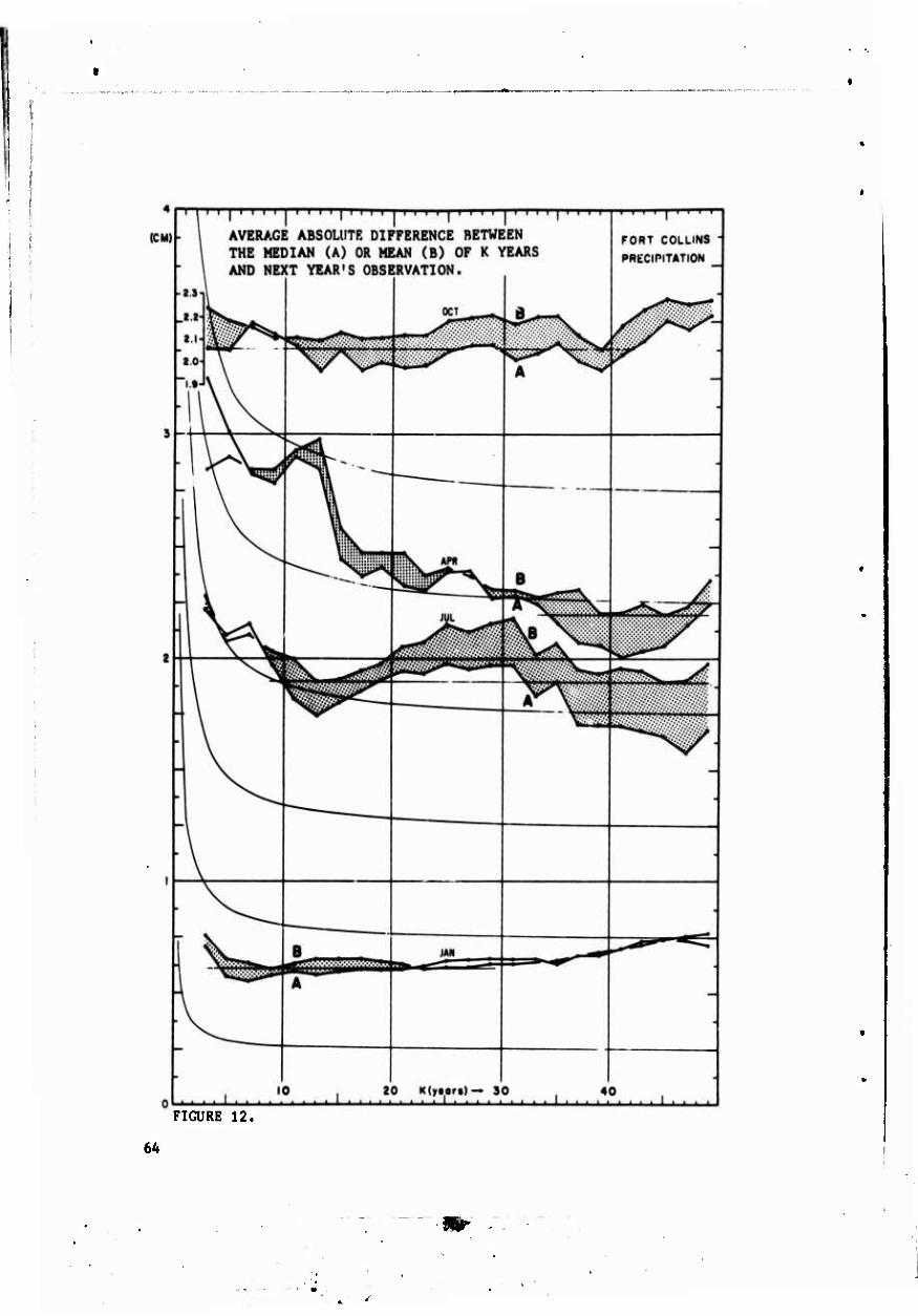
FIGURE 12.

64

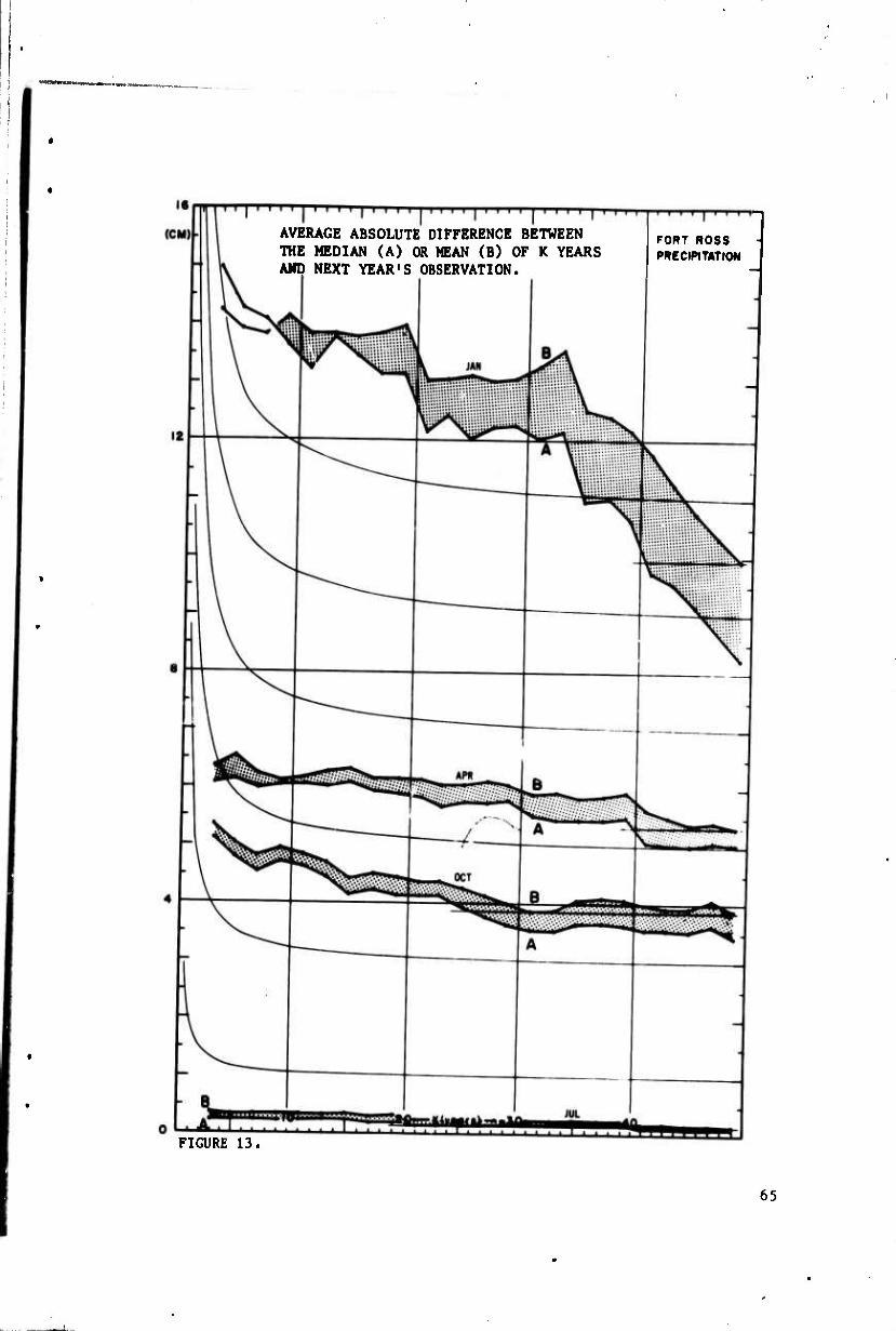
AVERAGE ABSOLUTE DIFFERENCE BETWEEN THE MEDIAN (A) OR MEAN (B) OF K YEARS AMD NEXT YEAR'S OBSERVATION.

FORT ROSS PRECIPITATION

FIGURE 13.

65

K

5-H DODGE CITY Annual Prtcipitation

12 3 4 M—*

FIGURE 14.--EXTENSION

6 10

66

**

CHAPTER V

CONCLUSIONS

In climatology, as in many other areas of geography,

it is often necessary to characterize entire sets of obser-

vations by a single value. In the past the arithmetic

average, or mean, has been the most generally used value.

Many variables have values that have the opportunity for

downward variation strictly limited by zero, while upward

variations are theoretically unlimited. Yet it is the

lower values that dominate the geography of an area. Here

the use of the mean is particularly at fault.

The arithmetic mean has been shown by the many map&

contained in this thesis to be a questionable, or at least

misleading, descriptive value. The arithmetic mean has

been hitherto employed as a measure of central tendency for

convenience of description. The indubitable advantages of

the arithmetic mean are the ease with which it is calcula-

ted (at least before the advent of the computer), and the

fact that the sum of the twelve monthly normals is equal to

the average of annual totals. Its chief fault lies in the

fact that equivalence of weight is given to each unit by

which an individual record departs from the mean.

Climates are not constant in position and it is falla-

cious to regard them as being so. The search for any valid

mean expression would seem foredoomed to failure. Climatic

statistics must therefore be examined in their entirety,

67

and obsolete normals must be replaced by indices of proba-

bility, as exemplified in the Atmospheric Humidity Atlas —

Northern Hemisphere (Gringorten et al,, 1966) . The first

step toward this goal would be to replace the arithmetic

mean with the median.

Many studies are liable to the biased errors inherent

in the arithmetic mean and the temptation to beg the whole

question when phenomena are submitted to subjective examin-

ation. Neither of these dangers would seem to offer much

difficulty when squarely faced; but tho more elaborate and

refined the subsequent analysis, the easier it is to over-

look initial limitations.

The present notion that the mean value is something

that will recur, or that it is the value which best repre-

sents what we expect to happen again, should be replaced.

The knowledge that the mean is only one measure of central

tendency, and a poor one at that when considering many of

the climatological variables, supports such replacement. In

the future it is hoped that summaries of climatological data

will feature the median along with, or instead of, the mean.

Climatology is not the only subfield of geography

where skewed distributions are encountered. Many geographi-

cal distributions are singly or doubly bounded and since

geographers are interested in reducing large amounts of data

to representative values which can then be used to describe

an area or compared with other values, it is of the utmost importance that the values are comparable and best estimate

68

the actual distribution. While the moan may have ^ome

computational advantages, it still fail'-, to represent the

most typical value in many distributions. This failure

has been recognized tor a few extremely skewed distribu-

tions, and the median values are now in general use to

represent 'average' income and 'average' number of yearn

of education. But the arithmetic mean continues to be used

to portray values of agricultural, industrial, and mineral

production; to indiu.jte consumption of goodr; to summarize

climatic condition'.; and many other variables which might

be better portrayed by the median.

69

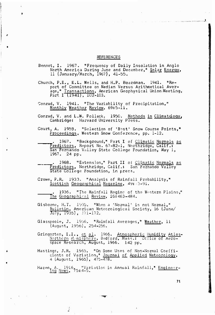
REFERENCES

Bennet, I. 1967. "Frequency of Daily Insolation in Anglo North America During June and December," Solar Energy, 11 (January/March, 1967), 41-55.

Church, P.E., E.L. Wells, and H.P. Boardman. 1941. "Re- port of Committee on Median Versus Arithmetical Aver- age," Transactions, American Geophysical Union Meeting, Part I (1941), 102-103.

Conrad, V. 1941. "The Variability of Precipitation," Monthly Weather Review. 69:5-11.

Conrad, V. and L.W. Pollack. 1950. Methods in Climatoloqy, Cambridge: Harvard University Press.

Court, A. 1953. "Selection of 'Host' Snow Course Points," Proceedings, Western Snow Conference, pp. 1-12.

. 1967. "Background," Part I of Climatic Normals as Predictors, Report No. 67-82-1, Northridge, Calif.: San Fernando Valley State College Foundation, May 1, 1967. 24 pp.

, 1968. "Extension," Part II of Climatic Normals as '""'Fredictors, Northridge, Calif.: San Fernando Valley

State College Foundation, in pre^s.

Crowe, P.R. 1933. "Analysis of Rainfall Probability," Scottish Geographical Magazine. ^9:/3-9i.

1936. "The Rainfall Regime of the Western Plains," The Geographical Review. 26:463-484.

Gisborne, H.T. 1935. "When a 'Normal' is not Normal," Bulletin, American Meteorological Society, 16 (June/ July, 1935) , 171-172.

Glasspooie, J. 1956. "Rainfall Averages," Weather. 11 (August, 1956), 254-256.

Gringorten, I.I. , et_ al. 1966. Atmospheric Humidity Atlas- Northern Hemisphere, Bedford, Mass.: office of Aero- space Research, August, 1966. 142 pp.

Hastings, J.R. 1965. "On Some Uses of Non-Normal Coeffi- cients of Variation," Journal of Applied Meteorology, 4 (August, 1965), 475-478.

Hazen, A. 1916. "Variation in Annual Rainfall," Engineor- Inq News. 1b:4-o. —J

71

*> »*WwtJ .vw.4". «.■-«.,...,

Hellman, G. 1909. Veröffentlichungen Preuss. Met. Inst. 3, No. 1 as quoted by V. Conrad and L.W. PoTTak in Methods in Climatology. Cambridge: Harvard Univer- sity Press, 1950. p. 56.

Hershtield, D.M. 1962. HA Note on the Variability of Annual Precipitation," Journal of Applied Meteorology, 1 (December, 1962), 575-57^

Joos, L.A. 1960. "Mean vs. Median in Weekly Precipitation',' paper read at 3r^ Conference on Agricultural Meteor- ology, Kansas City, Mo.: May, 1960. 5 pp.

. 1964. "Variability of Weekly Rainfall," Weekly Werther and Crop Bulletin. 51 (June 29, 1964), 7-8.

Kangieser, P.C. 1966. "The Use of the Mean as an Estimate of 'Normal* Precipitation in an Arid Area," U.S. Weather Bureau Western Region, ESSA, Western Region Technical Memorandum No. 15 (November^ 1966). 4 pp.

Landsberg, H. 1947. "Critique of Certain Climatological Procedures," Bulletin. American Meteorological Society, 28 (April, 1947), 187-191.

1951. "Statistical Investigations into the Clima- tology of Rainfall on Oahu (T.H.)," Meteorological Monographs. 1 (June, 1951), 7-23.

Lackey, E.E. 1935. "Annual Variability Rainfall Maps for Nebraska," Monthly Weather Review. 63:79-85.

1936. "A Variability Series of Isocrynal Maps of Nebraska," The Geographical Review. 26:135-138.

. 1937. "Annual-variability Rainfall Maps of the """""^üreat Plains," The Geographical Review. 27:665-670.

1942. "Reliability of the Median as a Measure of """""■^Rainfall," The Geographical Review. 32:323-325.

Longley, R.W. 1952. "Measures of the Variability of Pre- cipitation," Monthly Weather Review. 30:111-117.

Mathews, H.A. 1936. "A New View of Some Familiar Indian Rainfalls," Scottish Geographical Magazine. 52:84-9'.

McClean, W.N. 1956. "January Rainfall," Weather, 11 (January, 1956), 17.

Mindling, G.W. 1940. "Do Climatological Av--?rage^ Serve Adequately as Normals?" Bulletin, Auwri.on Metenro- logical Society, 21 (J- nTä'ry,' T94C.) , 3-6.

72

U.S. Department of Commerce, Weather Bureau, Monthly Total Precipitation," sheets of Atlas of the United States.

"Normal the National

West, G.G. 1940. "Minutes of the Regional Meeting of the Section of Hydrology, American Geophysical Union, at Seattle, Washington, June 20-21, 1940," Transactions, American Geophysical Union, 21:1053.

73

w

. I

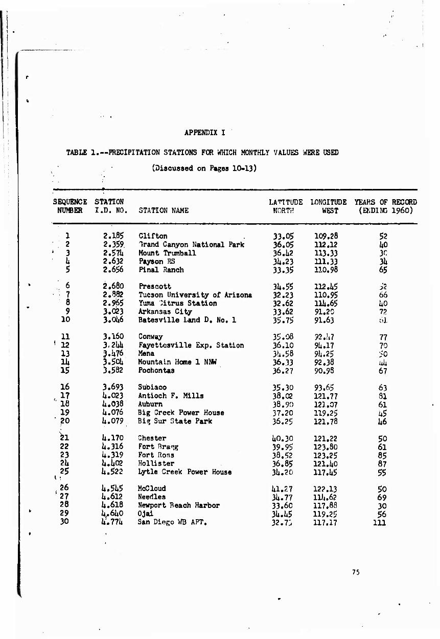
APPENDIX I

TABLE 1.—PRECIPITATION STATIONS FOR WHICH MONTHLY VALUES '/«RE USED

(Discussed on Pages 10-13)

SEQUENCE STATION NWBER I.D. NO. STATION NAME

LATITUDE LONGITUDE YEARS OF RECORD NORTH WEST (EKDIND i960)

1 2.185 Clifton 33.05 109.28 52 2 2.359 Irand Canyon National Park 36.05 112.12 1*0 3 2.57li Mount Trumball 36.1i2 113.33 3C h 2.632 Psyson RS 3U.23 111.33 3U 5 2.656 Final Ranch 33.35 110.98 65

6 2.680 Prescott 3U.55 112.1*5 52 7 2.882 Tucson University of Arizona 32.23 110.95 66 8 2.965 Yuma Citrus Station 32.62 llli.65 1*0 9 3.023 Arkansas City 33.62 91.20 7?.

10 3.01*6 Batesville Land D. No. 1 35.75 91.63 61

11 3.160 Conway 35.08 92 Ml 77 12 3.2U Fayettesville Exp. Station 36.10 91*. 17 70 13 3.1J76 Mena 3U.58 9l*.25 50 1U 3.501; Mountain Home 1 NNW 36.33 92.38 al* 15 3,582 Pochontas 36.27 90.93 67

16 3.693 Subiaco 35.30 93.65 63 17 iu023 Antioch F. Mills 38.02 121.77 31 18 li.038 Auburn 38.90 121.07 61 19 U.076 Big Creek Power House 37.20 119.25 u5 20 U.079 Bi» Sur State Park 36.25 121.78 1*6

*1 U.170 Chester Ii0.30 121.22 50 22 i4.3l6 Fort Bra^g 39.95 123.80 61 23 U.319 Fort Rons 38.52 123.25 85 2h U.Ü02 Hollister 36.85 121.1*0 87 25 U.522 Lytle Creek Power House 3U.20 117.1*5 55 26 k.SM McCloud hl.Zl 122.13 50 27 U.612 Needles 31*. 77 ID*.62 69 28 U.618 Newport Beach Harbor 33.60 117.88 30 29 U,.61i0 Ojai 3l*.li5 119.25 56 30 ii.m San Diego WB APT. 32.7: 117.17 111

75

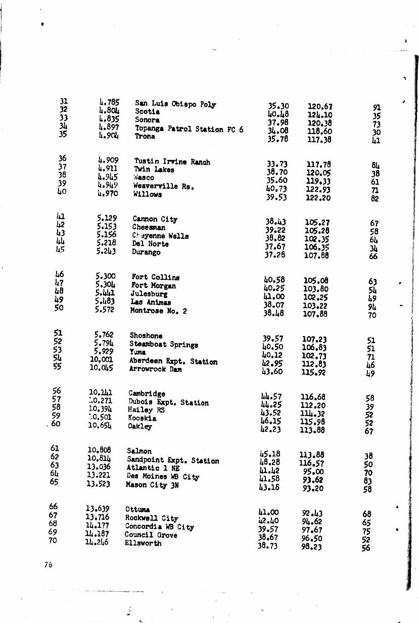
31 32 33 3U 35

li.785 San Luis CJbiapo Poly li.80ti Scotia li.835 Sonora Ii.897 Topanga Patrol Station FC 6 k»9Cii Trona

35.30 ao.us 37.98 31.08 35.78

120.67 12U.10 120,38 118.60 117.38

91 35 73 30 Ul

36 37 38 39 UO

h.909 Tustin Inrine Ranch ii.913 Twin Ukes li.9U5 Wasco k.9k9 Weavenrille Ra, l4.970 Willows

33.73 38.70 35.60 liO.73 39.53

117.78 120.05 119.33 122.93 122.20

8U 38 61 71 82

Ul U2 U3 hh U5

5.129 Cannon City 5.153 Cheesman 5.156 Or ayenne Wells 5.218 Del Worte 5.2li3 Durango

38.U3 39.22 38.82 37.67 37.26

105.27 105.28 102.35 106.35 107.88

67 58 6U 3h 66

1x6 h7 U8 U9 50

51 52 53 Sh 55

5.300 Fort Collins 5.30U Fort Morgan 5.1iUl Julesburg 5.1(83 Las Aninas 5.572 Montrose Mo.

5.762 Shoshone 5.79U Steamboat Springs 5.929 Yuna

10.001 Aberdeen Expt. Station 10,0li5 Arrowrock Dan

IiO.58 1*0.25 la.oo 38.07 38.1*8

39.57 1*0.50 1*0.12 1*2.95 1*3.60

105.08 103.80 102.25 103.22 107.88

107.23 106.83 102.73 112,83 115.92

63 51* 1*9 91* 70

51 51 71 1*6 1*9

56 57 58 59 60

10. ua :L0.271 10.391* 10.501 10.651*

Cambridge Dubois Expt. Hailey RS Kooskia Oakley

Station UU.57 1*1*.25 1*3.52 1*6.15 1*2.23

116.68 112.20 111*.32 115.98 113.88

58 39 52 52 67

61 62 63 6I4 65

10.808 Salmon 10.811* Sandpoint Expt. Station 13.036 Atlantic 1 NE 13.221 Des Meines WB City 13.523 Mason City 3N

1*5.18 1*8.28 1*1.1*2 1*1.58 1*3.16

113.88 116,57 95,00 93.62 93.20

38 50 70 83 58

66 67 60 69 70

13.639 Ottuma 13.716 Rockwell City 114.177 Concordia WB City H*.187 Council Grove ll*.2l46 Ellsworth

1*1.00 ia,ho 39.57 38.67 38.73

92 .U3 9U.62 97,67 96.50 98,23

68 65 75 52 56

76

i

71 1U.376 Hoiton 72 lU.Ui2 La Cycrne 73 lli.517 Medicine I.o(»rie 7h lli.637 Phillipsburg 75 IhM Plains

76 lU.66h Quinter 77 1U.731 Sedan 78 1U.731 Sedfrwick 79 1U.819 Toronto 80 I6.iai Calhour, Expt. Station

81 16.^70 Jennin^r 82 16.612 Melville 83 16.666 New Orleans WB City- 81i I6.73li Plain Dealing 85 16.892 Tallulah Delta Lab.

66 23.130 Capringer Mills 87 23.158 Chillicothe 25 88 23.223 Dexter 89 23.250 Eldon 90 23.282 Fayette

91 23.30li Fredericktown 92 23.379 Hermann 93 23.598 Neosho 9h 23.772 Shelbina 95 23.071 Warrensburg

96 23.899 Willow Springs 97 2U.G36 Augusta 98 2U.OU3 lallnntine 99 2h.077 Tig .Sandy

100 2h.l0h Rozeman Apri, College

101 2Ü.260 East Anaconda 102 ?'i.269 Ekalaka 103 2U.31ii Fortino Inne lOii 2U.389 Hamilton 105 2U.398 Haugan

106 2U.1452 Jordan 107 2ii.529 Lustre a NNW 108 2U.576 Moccasin Expt. Station 109 2a.729 Saint Ignatius 110 2a.881 West Slacier

39.a7 38.35 37.27 39.77 37.27

95.73 9a. 77 98.58 99.32

100.58

39.07 37.12 37.92 37.80 32.52

100.23 96.17 97.a3 95.95 92.33

30.23 30.68 29.95 3?.9C 32. ao

92.67 91.75 90.07 93.68 91.22

37.80 39.75 36.80 38.35 39.15

93.80 93.55 89.97 92.58 92.68

37.57 38.70 36.G7 39.68 33.77

90.30 91.15 9a.37 92.05 93.73

36.98 a?Ji8 a5.95 a^.i? a5.67

91.97 112.38 108.13 110.12 113.05

a6.io a^.97 aö.73 a6.25 a7.36

112.92 ioa.53 lia.90 na.i1; 115.ao

U7.12 as.as a7.05 a7.32 a;i.Fr

106.90 105.93 109.95 llu.lO

as 30 68 69 51

30 76

6a 69

63 7a 91 67 a3

3a a3 37 57 V6

36 86 73 • 7 77

37 <a ai 37 58

55 56 39 33 a8

30 39 30 52 35

77

i

111 112 113 lilt 115

25.093 25.115 25.202 25.280 25.302

Blair Brldgo Port Cret« Ewlng Port Roblnaoa

1*1.55 1*1.67 1*0,62 1*2.25 1*2.67

96.13 103.10 96.95 98.35

103.1*7

91 63 81 68 77

116 117 118 119 120

25.318 25.363 25.697 25.701* 26.005

Oenoa Hwtington Purdum Rarenna Adaren

1*1.1*5 1*2.62 1*2.07 1*1.03 38.12

97.73 97.27

100.25 98.92

115.58

85 69 58 83 1*2

121 122 123 121» 125

26.257 26.517 26.678 29.152 29.181

Elko VO Apt. Ming Reno WB Apt. Carrisoso Clmarron

1*0.83 38.38 39.50 33.65 36.52

115.78 118,10 119.78 105.88 101*. 92

91 53 90 52 57

126 127 128 129 130

29.191* 29.285 29.327 29.378 29.1*71*

Clevis Ellda Port Bayard Hachlta Lake Avalen

3l*.l*0 33.95 32.80 31.92 32.1*8

103.20 103.65 108.15 108.32 10l*.25

1*9 1*5 90 51 1*6

131 132 133 13ii 135

29.668 29.851* 29.990 32.219 32.362

Pecos RS State university Zunl FAA AP. Dickeneon Expt. Station Orand Porks U.

35.58 32.28 35.10 1*6.88 1*7.92

105.68 106.75 108.78 102.80 97.08

37 100

1*6 69 69

136 137 138 139 11*0

32.1*1*2 32.561* 32.602 3U.350 31*.1*1*5

Jamestown St. Hosp. Max Mohall Oeary Idabel

1*6.88 1*7.82 1*8.77 35.63 33.90

98.68 101,30 101.52 98.32 9U.82

68 30 67 1*9 31*

11*1 11*2 11*3 11*1* 11*5

31*.1*77 3l*.693 31*. 701 31*.91*5 31*.963

Kanten Pauls Valley Perry Webber Falls Wichita Mt. Wir

36.92 3U.75 36.28 35.52 3U.73

102.97 97.22 97.28 95.13 98.72

60 57 30 62 1*5

li*6 11*7 11*8 11*9 150

35.020 35.069 35.190 35.211* 35.269

Antelope IN Bend Cottage Irovs 1 S Danner Estaehada 2 SE

I*l*.92 1*1*.07 1*3.78 1*2.93 1*5.27

120.72 121.32 123.07 117.33 122.32

36 50 1*1* 30 52

78

m

151 152 153 I51i 155

156 157 158 159 160

161 162 163 16U 165

166 167 168 169 170

171 172 173 171» 175

176 177 178 :79 3 80

181 182 183 18U 185

186 187 188 189 190

35.3U* Grants Pass 35.383 Heppner 35.U67 Lakeview 35.561 Minam 7 NE 35.691 Prospect 2 SW

35.725 Rock Creek 35.905 Wann Springs Reservoir 39.030 Amour 39.197 Cotton Wood 39.280 Eureka

39.383 Hiehmore 1 W 39.U01 Hot Springs 39.1i66 Ladelle 7 NE 39.U86 Lerrmon 39.551i Milbank

39.767 Sioux Fall WB AP 39.855 Vale 39.9liU Wood m.012 Albany lil,050 Balmorhea Exp. Station

al.06l Beaunont Ul.llli Brownwood iil.202 Corsicana U1.318 Flatonia Ul.3li3 Jalveston WB City

m.35l George West U1.373 Greenville 2 SW lil,Ü08 Henderson UHi78 Kerrville 1*1.50? Lanrasas

Iil.597 Mission lil.695 Perry ton U1.721 Post U1.726 Presidio )i 1.765 Riverside

1*1.863 Sterling City U1.928 Valley Junction lil.933 Vega Ul,953 Weatherford ii2.210 Deseret

U2.1*3 U5.33 U2.18 U5.68 U2.73

123.32 119.55 120.35 117.60 122.52

U*.75 U3.57 ii3.32 ^3.97 hs.n

118.08 118.20

98.35 101.87 99.62

IiU.52 i43.U3 hk.68 U5.93 1*5.22

99.h7 103.1*7 98.00

102.17 96.63

U3.57 hh.62 1*3.50 32.73 31.00

96.73 103.1*0 100.1*8

99.30 103.68

30.08 31.72 32.03 29.68 29.30

91*.10 98.98 96.1*7 97.1C 91*.83

28.35 33.12 32.15 30.03 31.05

98.12 96.13 91*. 80 99.13 98.18

26.22 36.Ü0 33.20 29.55 30.85

98.32 100.02 101.37 101*.1*0 95.1*0

31.85 30.83 35.25 32.75 39.28

100.98 96.63

102.1*3 97.80

112.65

72 55 U8 51 53

hi 30 63 51 52

58 57 61* W* 71

70 52 1*8 79 37

68 68 75 53 89

1*5 59 52 65 66

1*0 1*8 1*1* 30 57

30 58 30 67 61

79

I I

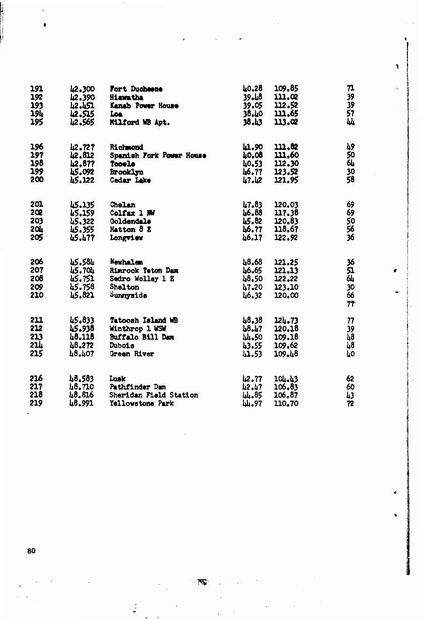
191 192 193 19U 195

U2.300 U2.390 U2.U51 U2.515 U2.565

Port DuohMM Hlamtha Kanab Powr Hous« LM Mllford MB Apt.

U0.28 39.U8 39.05 38.UO 38.1i3

109.85 111.02 112.52 111.65 113.02

71 39 39 57 hk

196 197 198 199 200

U2.727 U2.812 U2.877 U5.092 U5.122

RichBumd Spanish Pork Ponor Houa« Tooel« Brooklyn Cedar Lakt

la.90 UO.OS U0.53 Ii6.77 U7.U2

111.82 111.60 112.30 123.52 121.95

1*9 50 61* 30 58

201 202 203 201* 205

U5.135 U5.159 U5.322 U5.355 U5.U77

Chelan Coif ax 1 Iftf Ooldendala Hatten 8 E LongTiow

U7.83 U6.68 U5.82 U6.77 U6.17

120.03 117.38 120.83 118.67 122.92

69 69 50 56 36

206 207 206 209 210

U5.58U U5.70U U5.751 U5.758 U5.821

Newhalen Rimrock Teton Dan Sedro Wolley 1 E Shalton ^unnysid«

U8.68 U6.65 U8.50 U7.20 U6.32

121.25 121.13 122.22 123.10 120,00

36 51 61* 30 66 n

211 212 213 21ii 215

U5.833 45.938 U8.118 U8.272 U8.1i07

Tatooah Island WB Winthrop 1 WSW Buffalo BUI Dsm Dubols Qreen River

U8.38 U8.1»7 U4.50 U3.55 U.53

12U.73 120.18 109.18 109.62 109.U8

77 39 i*8 kB ho

216 217 218 219

U3.583 U8.710 U6.816 U8.991

Lusk Pathfinder Dam Sheridan Field Station Yellowstone Park

li2.77 U2.U7 Ui.85 lil*.97

10U.U3 106.83 106.87 110.70

62 60 ii3 72

80

^

CLIMATIC PREDICTION

Optiimun Length of Record

1» Origin of Program

This program was prepared in the Climatology Laboratory of San Fer-

nando Valley State College, Northridge, California by Paul £. Roy, Jr. and

Williaa F« Slusser as part of Air Force Project "Optimum Record for Clima-

tic Estimation and Prediction,n to assist in the analysis of climatic data

to determine the optimum length of record for climatic prediction.

2. Purpose of Program >

This program accepts monthly and yearly data in varied formats (Sec. 5)

and computes the extrapolation variance, S(k,m), the absolute prediction

error using the mean, Q(k,ra), and the median, D(k,m; for varying k year

periods and observations m years ahead. It then finds the optimum length

of record (k*) for each of these and computes F(k,m), QF(k,ra), and DF(k,m},

the percentage difference between the value obtained at k* and that found

using the other values of k«

3« Description of Equipment

Ihls program was developed for use on the IBM 360/75 # but can be used

on most computers using Fortran IV«

k» Method of Computation

a» S(k,ra) is obtained by averaging the squared differences between

the mean of k successive observations and an observation n ye?rs later for

which the value is to be estimated from that for the k years.

81

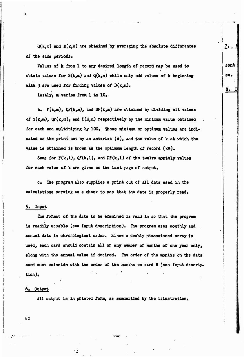
Q(k,ra) and D(k,m) are obtained by averaging the absolute differences

of the sane periods«

Values of k from 1 to an/ desired length of record ma/ be used to

obtain values for S(k,m) and Q(k,n) while only odd values of k beginning

with 3 are used for finding values of 0(ktm)«

Lastly» m varies from 1 to 10«

b« F(k,m), QF(k,m), and DF(k,m) are obtained by dividing all values

of S(k,m), QF(k,m), and D(E,m) respectively by the mlninun value obtained

for each and multiplying by 100« 'fliese minimum or optimum values are Indi-

cated on the print out by an asterisk (*), and the value of k at which the

value Is obtained is known as the optimum length of record (k*)«

Sums for F(k,l), (iF(k,l), and DF(k,l) of the twelve monthly values

for each value of k are given on the last page of output.

c« The program also supplies a print out of all data used In the

calculations serving as a check to see that the data Is properly read«

$> Input

The format of the data to be examined is read In so that the program

Is readily ucoable (see Input description)« The program uses monthly and

annual data in chronological order« Since a doubly dimensioned array is

used, each card should contain all or any number of months of one year only,

along with the annual value if desired« The order of the months on ths data

card must coincide with the order of the months on card B (see Input descrip-

tion),

6« Output

All output Is In printed form, as summarized by the illustration«

It. n

82

'

7> Oporatln^ Instructions

Standard Fortran IV Is used» No sense switches are used. At the pre-

sent the program does not handle tapes, but It can be easily modified .to do

SO«

6» Description of Terwa

IN - physical input unit

IOUT - physical output unit

NST - the symbol for denoting the minimum value

NBL - the symbol denoting other than minimum value

XHON(I) - thirteen three letter words: Jan, Fab, • • «Sum; or Tr

KM/UC - the maximum value of k

N - the number of observations per month (or year)

ISETS - the number of sets of data per card

NN/IME(I) - the name of the station, the variable, and the years

of record

FMT(I) - the format of the data being read in

X(L,NH) - value of observation, monthly or annual

SDF(K) - sum of poathly values of IF(k,m)

SAF(K) - sum of monthly values of QF(k,m)

SF(K) - sum of monthly values of F(k,m)

• IMIN(M) - minimum value of Q(k,m)

XHIN(M) • minimum va lue of S(k,m), SQ or D(k,m)

X(J) - the moan or median value of a k year period

SSUKL - sum of absolute differences using mean

SSUM - sum of absolute differences using median or squared

differences ur-Jng wean

S(K,M) - extrapolation variance or absolute prediction error

using mean 83

Q(K;M)

LOC(N)

NBUNK(K,N)

MBUNK(K,M)

Z(MID)

• th« absolut« prediction error using the asan

• the ▼alue of k where NST le to be placed

• the synbol to be printed after each ralue of S(k,a),

SQ or D(k,a)

- the ejrnbol to be printed after each value of Q(k,n)

- the median of k years

IXMH JDiME! DU

INPUT DESCRIPTION

A« One card containing an asterisk (*) in the first coluan«

B« One card containing the names of the months using columns

1 through 36« three columns per month* If annual data is

included« sum or yr should be punched in columns 37 through

39.

C« One card containing the maxlraum value of k desired in

columns 1 through 3j the number of years of record in

columns U through 6; the number of sets of obserrations (13

if all months and the annual amount are included) in columns

7 through 8; and the station naiw, variable name, and date

of beginning and end of observations in the remainder of the

columns«

0« One card containing the format of the data in the first 60

columns«

2« Data

F* Each successive group of data requires only cards C and D«

-_

84

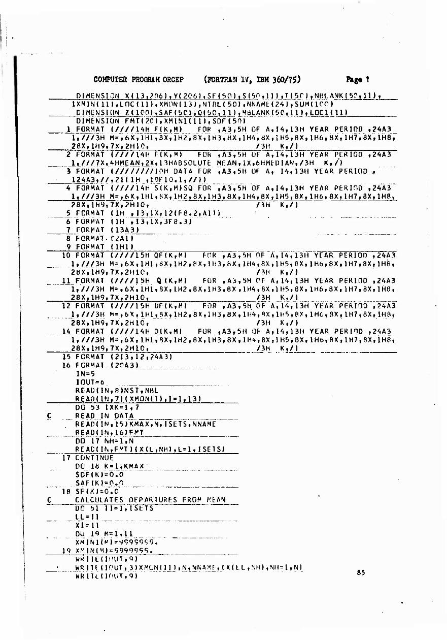
COMPUTER PROGRAM ORCEP (FORTRAN IV, IBM 360/75) ^g« 1

DIMENSION X(I3,?06)>Y(206)tSF(e»0)tS(50 ,1 1 )_,J_( ST ), NBI. WKl5?,ll)t 1XMIN( 11», LOC(11)t XMON(13),NT BL(50)»NNAHt(24),SUM(1CÖ )

__P1MI:NSHJN Z(lCn),SAF(5)C),0(t)0,ll),MbLANK(50,ll )f L0C1CU) DIMENSIÜN rMr(20),XMINl(lI»,SOF(50)

I FORMAT (////14H F(K,M) FOR tA3,5H l)F AfI4,13H YEAR PERIOD f24A3 1,///3H M=",6X, lHl,aX»lH2,8XfiH3,«XflH4f 8X,lH5,8X,lH6f 8X,lH7,8Xf lH8r 28X(lH9t7Xt?H10f /3H K,/)

2 FORMAT l////\4H r(K,M) FOR fA3,5H UF A,K,13H YEAR PfRIOO ,24A3 __lt''//7Xt^HMEANf_2Xf 13HAßSDLUT£ ME AN, IX,6HMtÜ IAN,/3H K,/» 3 FORMAT (////////IPH DATA FÜR ,A3,5H OF A, K,]3H YEAR PERIOD .,

_124A3,//,21( 1H tlOFlO.l,//)} 4 FORMAT {////IAH S(K,M)SQ FOR ,A3f5H OF AfI4,13H YEAR PtRIHO ,24Ä3 1,///3H M-,6X, IH1,8X,IH2f8X,1H3,8X,1H4,SXf1H5,8Xy1H6,SX,1H7,8X,1H8» 28X,lH9,7X,2H10f /3H K,/)

5 FCRMÄT (IH iJStlX, 12(F8.2,Ani 6 FORMAT (IH ,I3fIX,3F8.3) 7_ FORMAT (13A3)

'8 'FORMAT- f2An 9 FORMAT (IH1)

10 FORMAT (////15H QF(KfM) FOR fA3,!>H OF A,I4,13H YEAR PERIOD f24A3 1,///3H M=,6XflHl,tiX,lH2,8X,lH3,6XllH4f8X,lH5fCX, lH6,8X,lH7,8Xf IH8, 2bXVlH9,7X,2HlC, /3H K,/)

_U FORMAT (////It)H Q(K,M) FOR ,A3,5H PF A, 14,13H YEAR PERIOD ,24A3 1,///3H M=,6X,1H1,8X,1H2,8X,1H3,8X,IHA,8X,1H5,8X,IH6,8X,1H7,8X,1H8, 28X,1H9,7X,2H10, /^H KL/J

12 FORMAT (////15H DECK,«» FÜR ,A3,5H ÖF A,IA,13H YEAR~PERIOD ^24A3 I,///3H M=f6X,lHl_f 9X, lH2,8X,lH3,8X,lH4,8Xf lh,>,8XllH6,9X, IH7,8X»1H8, "28X,lH9,7X,2Hld, /3H K,/)

14 FORMAT (////14H 0(K,M) FUR ,A3,5H OF A,I4,13H YEAR PERIOD ,24A3 l,///3H M=,6X,lHl,8X,iH2,8X,lH3,8X, IH4,8X,1H5,8X,lH6,flX,lH7,8X,lH8,

28X,1H9,7X,2H10, /3H K,/) 15 FORMAT (2I3,12,24A3) 16 FORMAT (2rA3)

IN=5 10UT=6 REAÜ(IN,8»NS'T,NBL READ(1N,7)(XM0N(I),1 = 1,13) DO 53 IXK=lf7 READ IN DATA REAr(IN,l5)KMAX,N,ISETS,NNAME

__ REÄD(INt16)FMT DO 17'NH=1,N READ(IN,FMT)(X(L,NH),L=1,ISETS)

17 CONTINUE DC 18 K = UKMAX SOFCKl'sO.O SAF(K) = 0JtO

18" SF(KI=Ö".0 CALCULATES J}EPARTURES FROM MEAN ÜO bl I 1 = 1, fSfcTS LL=II _

' X'l=II OÜ 19 M=l,ll XMlM(M)=S9999S9.

19 X1VIN(M) = 99999<;<;. W«IlE(lnUT,9) WRin (lOUT, 3)XMGN(n ),N,NNA.yr,(X(l.L,NH),NH=l,M WRnL(iriUT,9) 85

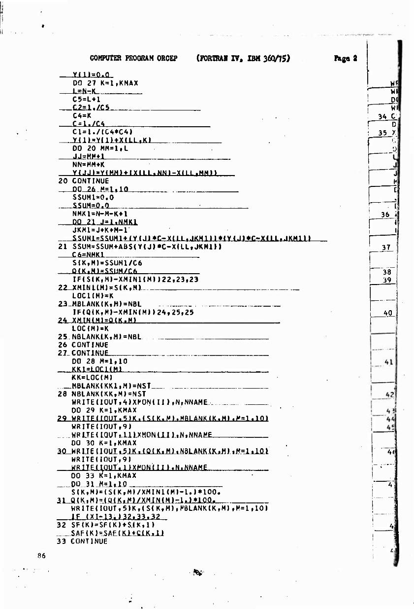
■ ■ «« 1-V* V-KV" .f-««»* ■* '

COMPUTER PROGRAM ORGEP (FORTOAI IV, IBM 360/75) Plage 8

vni^o.n DO 27 L=N-,

K=l,KMAX Wf

C5=L*1 -C2=UZC5. C4=K

Dt Wl

34 C

Cl=l./(C4*CA) Jtil L-jyiIltX(LL«KJ DO 20 MM=lfL

-J.iHMMÜ

r D i 35 x

NN=MM+K YUJ)=Y(MMl»mLL.NNI-Xm .MMH 20 CONTINUE D0_^i_^=.LiIQ

SSUMI=0.0 1SUM=0.0 :

NMKl = N-M-K-H DO 21 J=1.NMK1

JKMl=J+K*M-l s.suMi=ssuMi*ur_( ji*c-x{LLtJKMin*mji*c-xaLtJKMin 21 SSUM=SSUM+ABS(YUI*C-X(LLf JKMin c&=NMia

S(KVM)=SSUM1/C6 Q(KiM) = .SS»M/r.ft

IF(S(KtM)-XMINl(M))22t23,23 22_XMlNltMJ = S(K,M)

L0C1(M)=K 23_MBLANK(K.M)=NBL

IF{Q(KfMI-XMIN(M)»24,25,25 24 XJ1INlH)=Q(KtM>

3*:

37

1 1

r i 38 1 i 39

40

LOC<M)=K 25.NBLANMKfM)=NBL 26 CONTINUE 27_ CONTINUE

DO 28 M=l,10 KKULQCHMI KK«L0C<M)

.MBLANKi KK11M)=NST NBLANK(KKtM)=NST WRITE(I0UTf4)XP0N(II),NiNNAME DO 29 K=ltKMAX

29 HRITE([QUTt51K«(S(Ktf<)tMBLANK(KtM»iP=ltlQ>

28

WRITE(I0UT,9) __WPiJ£(IQJJTi_LllXMON.LULi^iNNAtiE

DO 30 K=l,KMAX aOLWRI.TE (IGUIi3)Ki (Q( KtAliNBLAMiJUM) ti?i=_lilO-l

WRITE(I0UTi9) WRITEUOUT. DXMONdn.N.NNAME

4<

DO DO.

33 31

'i i *

=l,KMAX

S(K,M)=(S(K,M)/XMINl(M)-l.)*100. 1L Jl (K i M) =J QiJ^xiU^LMl&L(ilJ-lt)*lQO.

WRITE(I0Urt5)K,(S(K,M)iHBLANK(K,M)tH=lt10) IF <XI-I3.n2t33t32

32 SF<KI = SF(K)«-S.(K,n SAP (K ) = SAF_( UltfilK^JJ 33 CONTINUE

86

**

COMPUTER FROQR1M ORCBP (FORTRAN 27, IBM 360/7^) *&iß 3

WRITE(I0UT«9) WRITHIOUTtlOXMONdnfMrNNAME DO 34 K^ltKNAX WRITE(IOUTf5IKf(0(K,H),NBLANKCK,M),M=l,10)

34 CONTINUE DO 35 M=lf10

35 XMIN(M>=999999S. CALCULATES DEPARTURES FROM MEDIAN DO 45 K=3tKMAX,2 L=N-K+1

J2=K MID=(K+l)/2 DO 40 JJ=lfL J5=J2-1 DO 36 J=J1,J2

36 Z(J) = X(LLfJ.> DO 39 in=Jl,MIO DO 38 J=J1,J5 IF(2(J)-ZU + 1)I38,38,37

37_H0LD=Z(JI ZTJI*Z(J*1I Z(J+l)=HOLD

38 CONTINUE 39 J5=J5-1

Y(JJ)=Z(MID) J1 = JU1

J2=J2+i 40 MIO=MIO*I

DO 44 MMtlO SSUM»0. NPKl = N-M-K-i-I

_ DO 41 J^LLN^KJ JKM1=J+K*M-1

41 SSUM=SSyM_tABSlYlJjj1X( LLt JKMl ) ) C2=N^K1

S(KtM)=SSUM/C2 IF(S(K,M)-XMIN(M))42f43,4 3

42 XMIN(M| = SiKf_MJ LCC(Mr=K

43 NBLANK(KfM)=NBL 44 CONTINUE 45 CONTINUE

00 46 M=lf iri KK=LOC(M)

46 NÖLANK([Kk,M)=NST WRITEdOUT^) WRltEnOUT, 14)XrtQN(II ),NfNNAHE DO 47 K = 3,KMAXt2 ^_^

47 WRlTE(I0UT,5)K,(S(KtM),NBLANK(K,M),H=l,10l WRITE(IÜUT,9J WRITEMOUT, 12)XMüN(n ),N»NNAME DO 50 K = 3,KMAXJL2 DO 48 M=l,10

48 S(KtM)=(S(KfMI/XMINIM»-1.1*100. ,M> ,^=1,10)

87

. WRIUnoUTt 5)K,(S(K,M)fNBLANK(K,M> ,^=1,10) IF (Xl-13.)49f50,49 __ _

49 SCF(K) = SOF(K)*S(K,h

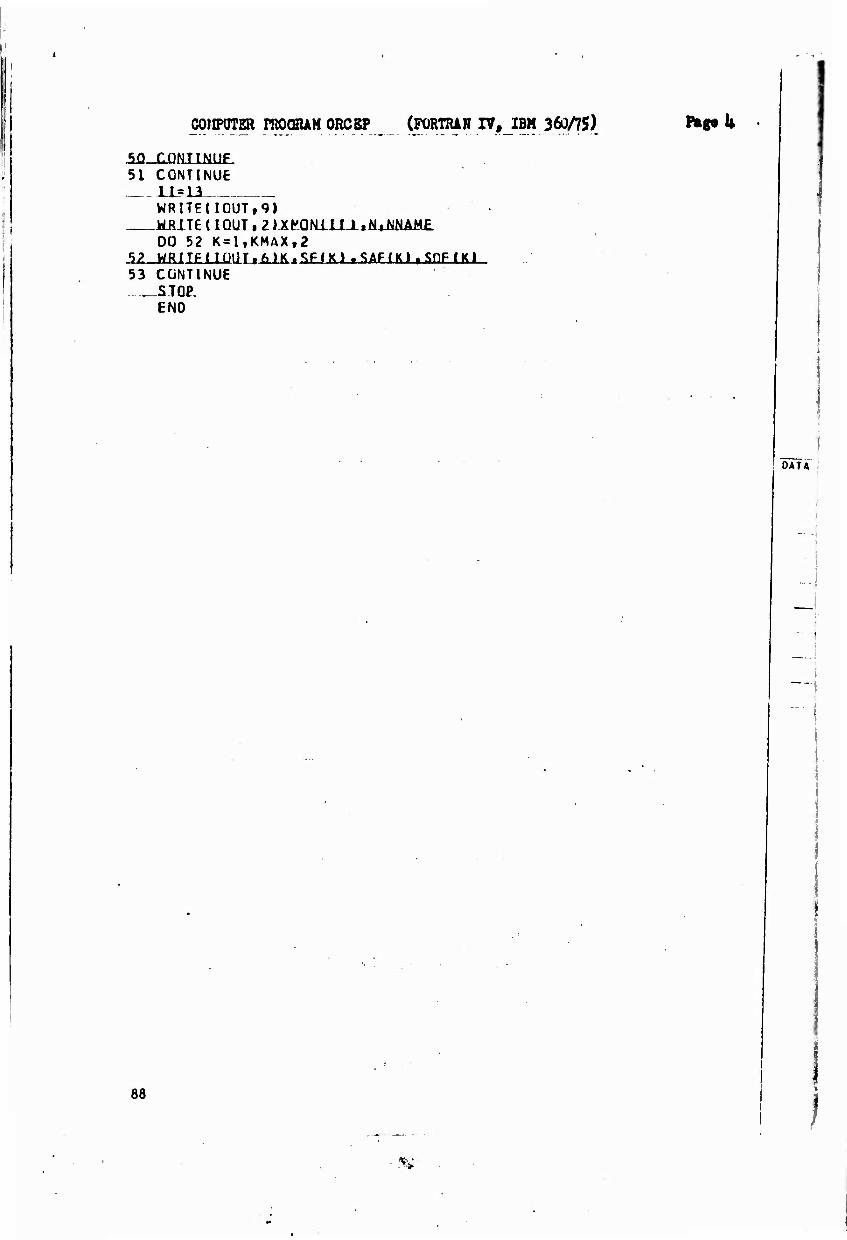
COMPUTER mOCfiUM ORCEP (FORTRAN IV, IBM 360/75) n&k

■SO f.nNTINUF. 51 CONTINUE 11=13

WRITE(IOUT,«n WJiiTE {IQUT, 2).XH0m.lU..N^NAM£

DO 52 K=1,KMAX,2 *)?. WRITF(IÜÜ.U61K,.: 53 CONTINUE STOP.

END

DATA

88

I %

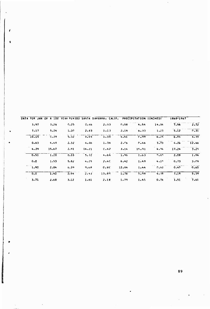
DATA FOR JAN C^ A IOC YEAR PtHiOD SANTA BARBARA, CALIF. PRECIPITATION (INCHES) 1868-1967

3.97 3.26 0.25 0.H6 2.53 n.58 4.54 14.9« 7.56 T.ff 7.17 5.24

C.29

1.30

'5.32'

2.83

0.45

1.13

"iTio

2.18 6.3 3 1.23 5.12 P.31

10.15 4.41 0.99 6.25 6.84 4.35

0.63 4.<.8 2.32 4,d6 1.36 2.r6 0.46 3 ^73 ^4.26 12.46

4.29 15.67 2.91 14.21 C.4? 3.14 15.91 ' 4.14 17.24 " T.25

0.51 1.20 0.33 5.J2 4.64 1.96 1.63 0.60 2.08 1.94

0.0 1.53 5.82 4.25 2.4C 6.42 1.49 4.1" 0.73 3.09

~ 1.90 2.84 6.39 9.6H

2. ^j'

0.8C

13.89

12.84 1.44 0.60 Ö.4Ö~ 0^60

0.0 1.40 2.54 1.78 5.98 4.19 7.19 5.39

3.71 2.68 3.12 1.81 2.18 1.79 1.45 0.76 1.51 7.61

89

SIK.M ISO FUR JAN OF A

2

100 YfcAR

3

PERIOD SAN

4

TA BARBARA , CALIF. PRECIPITATION <INCHES» 1*68-1067

N- I 5 6 7 8 1 10 K

33.06" "li.OQ 30. 19 1 29.95 21.22 30.80 30.58 34.35 30.86 32.73 2 18.26 18.50 ^4.4? 24.28 24.78 24.92 23.06 23.21 23.50 24.30 3 18.49 19.39 22.55 23.62 22.81 22.36 21.23 22.74 22.08 23.24 4 18.81 18.86 22.14 22.03 20.49 20.67 20.62 21.00 21.40 21.84 5 18.33 19.07 2C.96 19.73 19.22 20.11 19.67 20.45 20.47 21.34 6 18.60 18.60

16.85 18.97 18.13

18.78 18.60

19.01 18.43

19.39 19.16

19.45 19.03

19.86 19.76

20.31 19.77

20,60 7 18.19 2C.55 8 16.61 16.40

16.54 18.10 17.88

18.19 18.25

18.40 18.16

18.87 18.94

19.10 18.78

lt'.39 19.52

19.89 19.63

20.07 9 16.34 20.24

10 16.48 10.52 16.00 17.85

18.05 18.21

18.32 18.67 18.97 19.37 19.02 19.68 11 16.46 16.74 18.12 18. db 18.87 19.58 19.34 19.73 12 16.68 10.68 18.01 lb.02 18.34 18.81 19.09 19.18 19.39 18.77 13 16.01 16.9" 17.84 IP.23 18.33 19.01 18.76 19.21 18.51 18.88 14 16.85 16.84 18.08 18.24 1H.57 18.72 18.84 18.36 18.65 1H.<H 15 16.79 17.12 18.r") ie.47 18.33 18.80 18.03 18.50 1«.76 18.90 16 17.C8

17.13 17.18 17.40

18.34 18.14

IP.26 18.45 18.00 18.20 18.61 H.71 18.96 17 18.3? 17.66 18.15 18.31 18.58 18.78 18.82 IB 17.39

17.27 17.33 17.47

18.24 17.51

17.64 17.79

17.82 18.28 18.28 18.65 18.67 M.58

18.71 IS 17.94 18.26 18.37 18.54 18.74 20 17.41

16.74 10.81 17.00

17.07 17.81

17.94 17.96

17.95 18.06

18.36 10.30

18.30 18.27

18.4« 18.54

13.64 18.88 21 18.76 18.93 22 16.92 17.19 17.82 18.07 18.05 1H.27

18.36 18.37 18.52

18.7C 18.79

18.85 18.99

19.Of, 23 17.10 17.23 17.95 18.06 18.04 • o.r: 24 17.14 17.37 17.95 18.05 _18.15 _ 18.51 18.63 18.92 13.96 19.20 25 17.29 17.40 17.96 18.15 18.29 18.62 18.77 18.91 19.15 19.2" 26 17.32 17.43 18.06 18.28 18.41 18.78 18.77 19.11 19.17 19.40 27 17.37 17.55 18.20 18.41 18.57 18.79 18.98 19.13 19.33 19.33 28 17.48

17.64 17.70 18.34 18.58 18.59 19.00 19.01 1<».34 19.31 19.59

29 17.85 18.50 18.61 18.81 19.05 19.22 19.30 19.56 19.71 30 17.79 18.01 18.54 18.83 18.87 19.25 19.18 10.53 19.69 2C.05 31 17.95 18.07 18.76 18.90 19.07 19.21 19.41 19.67 20.03 19.Oi 32 18.01 If .29 18.83 19.n 19.06 19.45 19.55 20.01 19.00 19.15 33 18.25 18.39 19.04 is.n 19.29 19.6C 19.9C 18.99 l".!! 16.97 34 35

18.34 18.56

18.60 18.6 3

19.04 IS.28

I'i.ii 19.5iJ

19.46 19.80

19.95 18.94

18.97 19.00

19.11 16.93

16.9? 17.1 }

17.17 15.57

36 18.59 18.87 19.45 IS.85 18.78 19.07 16.80 17.14 15.5^ 15.51 37 18.84 19.06 I'i.bO 18.82 18.«52 lb.86 17.02 15.5^1 15.45 15.75 38 19.03 IV.40 18.74 18.96 16.67 17.07 15.35 15.47 15.69 13.03 39 19.38 18.36 18.89 16.71 16.89 15.40 15.i2 15.71 12.98 13.2? 40 18.34

18.50 18.51 16.37

10.66 ' 16. «"7 '

lfc.94 15.35

15.23 15.18

15.37 15.61

15.5b 12.96

13.01 13.23 9.Q6* 41 13.27 10.02* 1^.29 42 43

16.37 16.58

lb.59 15.12

15.30 15.22

15.30 15.54

15.42 12.96

13.02 13.30

13.21 10.17*

10.07* 10.39

n.3f 10.32

10.29 10.46

44 15.10 15.05 15.46 13.07 13.24 10.22* 10.49 10.35 n.49 1C.33 45 15.00 15.28 13.09 13.35 10.28* 10.54 10.42 10.49 in.iZ 10.65 46 15.23 12.88 13.37 IC.35* 10.59 10.48 10.57 10.34 10.63 10.76 47 12.83 13.16 10.35* IC.66 10.53 10.63 10.42 10.65 10.75 1C.87 48

10.22* 10.26* 10.56

10.65 10.56

IC.57 10.68

10.65 10.47

10.44 10.76

10.74 10.87

10.78 10.83 11.85

1C.P9 49 IP.86 10.81 M 10,50 10.42 10.63 1C.45 10.79 10.90 10.93 10.95 10.73 10.87

90

KkB

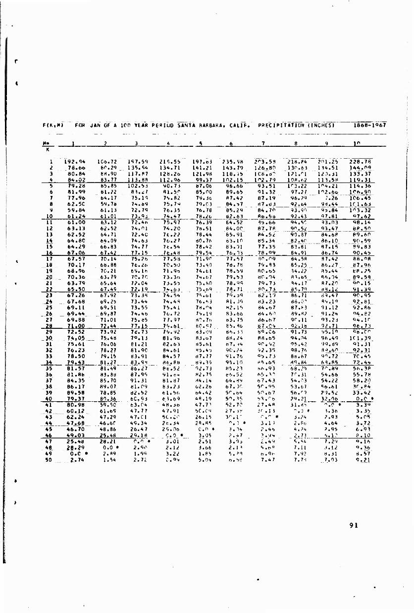
MKi H» FOH

1

JAN OF 4

2

ICO YEAR

3

P6ÖIU0 SANTA HAR8AKA, CALIF.

«56

PaECIPITATION (I

7 8

NCHCS) 1866-1967

*■ 9 1^ K

192. <H IC6.72 197.59 219.55 197.e3 235.98 203.59 218.P4 7nu2*5" 1 228.78 ^ 76.66 60.29 135.54 134.71 141.21 143.79 126.80 130.63 134.51 144.09 3 80.64 Brt.90 117.87 128.2b 121.98 116.(5 ICb.dO l>l.oi 121.31 133.37 4 84.02 83.77 113.HR 112.96 99.37 102.15 102.79 108.f.2 113.58 119.31 5 79.28 85.85 102.5i 90.7i 87.06 96.66 93.51 103.22 104.21 114.36 6 81.99 ax.zz 8^.^7 81.5^ 85.00 89.65 91.32 97.27 102.60 106.90 7 77.96 64.17 75.i<; 79.82 79.36 P7.42 87.19 96.29 7.26 1C6.45 B 62.5C 59.7» 7«..b9 75.79 79.03 84.■57 87.83 92.64 98.44 If 1.63 y 59.64 61.13 72.79 76.35 76.78 85.29 84.70 93.91 93.84 103.32

10 61.24 61.01 73.QJ 74.W 78.2t, 82.63 flb.5o 92.43 17.81 07.62 u 61.00 6.3.12 72.4* 75.97 76.39 64.52 It.bb 94.5C :>3.03 «58.14 12 63.13

62.52 62.52 64.71

74.01 72.4C

74.20 7t.22

78.51 78.44

84.or 65.91

87.78 84.52

90.52 93.47 eP.50

13 90.87 84.68 89.60 U 64. ec 64.09 74.63 76.27 d0.7ft o3.10 85.34 8 2.40 86.10 90.59 15 64.29 66.83 74.77 7t.54 78.42 8 3. T1 77.35 83.81 87.15 99.83 16 67.06 67.42 77.15 7t.4ö 79.54 76.13 78.09 84.91 36.74 90.45 17 67.57 70.14 75.26 77.58 71.90 7 7.57 '10.09 84.5« 97.42 88.OR 18 70.17 68.88 7t.26 7C.50 73.40 78. 78 79.q? 85.25 86.^7 87.96 19 66.96 70.21 tH.\h 71.9^ 74.61 78.59 80.65 14.22 85.44 tP.?5 2P 70.36 63.79 10.ir. 73.3f. 74.67 79.53 «0.04 81.65 86.14 89.59 21 63.79 65.64 72.04 73.55 75.80 78.99 79.73 "V4.17 8 7.20 90 . 16

?2 65.50 67.49 72.19 7^.03 75.69 78.71 90.73 as,7i «H.12 91.39 23 67.26 67.92 73.3H 74. 5<. 75.0 1 79.39 62.19 36.71 ri9.47 90.95

^2* 67.66 09.25 73.4^ 7'».4S 7b.'>J 81. 39 «3.23 88.0-1 99.10 92.81 25 69.11 69.51 73.55 75.M 7rt."4 M2. 15 84. b 7 87.M 91.12 92. R6

.26 69.44 69.87 iM.tb 7C.72 79.19 S3.66 «4.6"» 89.rt? 91.24 04. 8 2 27 69.88 71.01 75.85 77.97 H?.7(. 03. 75 86.67 90.11 93.2i <*4.1o

20 7ltoo 72.52

72.44 73.92

77.15 7ä.73

79.bl 79.92

80.^7 «3.09

85. It Ö7.C4 bi.Cb

92.1b 92.71 96. 73 29 91.73 95.1" Ob.C

_30 74.05 75.48 70.1J 81. 9b 83.o7 88.24 88.b5 94.04 96.49 1C1.39 31 75.61 76.06 81.21 82.bi 85.61 «7. ^4 90.92 95.42 99.89 91.31

32 76.23 78.27 61.9C 8 «..61 H5.4'j 90.24 92.35 98.76 99.60 92.31 33 78.50 79.15 83.91 84.57 87.77 91.76 "5.73 88.67 9^.72 7C.45 34 79.43

81.57 81.27 ei.49

83.9^ "86.2 7"

86.88 8e'.52

ö9, 35 " ^2.73

95.10 85.23

HS .65 r.6.9'3

89.84 69.85 72.44 35 68..'5 70.89 56.3P 3b 81.8b H3.8U 87.95 Sl.ti-4 P2.7'i es.52 65.^0 70.31 54.66 55.78 37 84.35 85.70 91.31 81.87 H4.14 64.^9 67.43 54.03 54.22 58.20

.38 86.17 89.07 81.09 83.2J 62.20 67. K 50. OS 53.6? 56.61 30.84 39 89.58 78.85 82.52 6 1.5/. 64.42 50.64 50.fa? 56.^9 29.52 33.42 40 79.37 80.36 6C.9J

63.04 63.69 «•8.30

4R.19 47.71

50.I«, 52.70

•33.^6 27.4«

?t».21 3i.H''

32.06 o.O »

O.C ♦ 41 80.98 59.50 3.34 42 60.12 61.69 47.77 47.91 5C.C9 27. i* .".15 ",■} * 5.36 3.35 43 62.24 47.29 4 7.C1 5C.:r 26.15 30. 1' .-.^ • 3.24 2.93 5.C5 44 47.66 46. 6C 49.34 2t.44 2R.H5 ". ) * 3.1 ? 2.r.o 4.64 3.72 45 46.70 48.86 26.47 2 9. nt, 0.0 ♦ 3.14 ?.46 4.24 ?.95 6.93 46 49.03 25.48 29.ia CO ♦ 3.05 2.47 ?.94 2.73 b.ir 8.10 47 25.48 28.21 O.o • 3.01 2.51 3.9J i.49 5.^4 7.29 0.I6 «L 28.29 0.0 • 2.90 2.12 3.66 2.1 ? S.p" 7.11 1.12 P. 36 49 O.C • 2.«9 1.9C 3.22 1.H5 5."1 o.9(- 7.93 Ö.31 8.57 50 _ 2.74 1.54 2.7£ C.'»9 5.0'« 0. 'it? 7.47 7.7-1 7.03 9.21

91

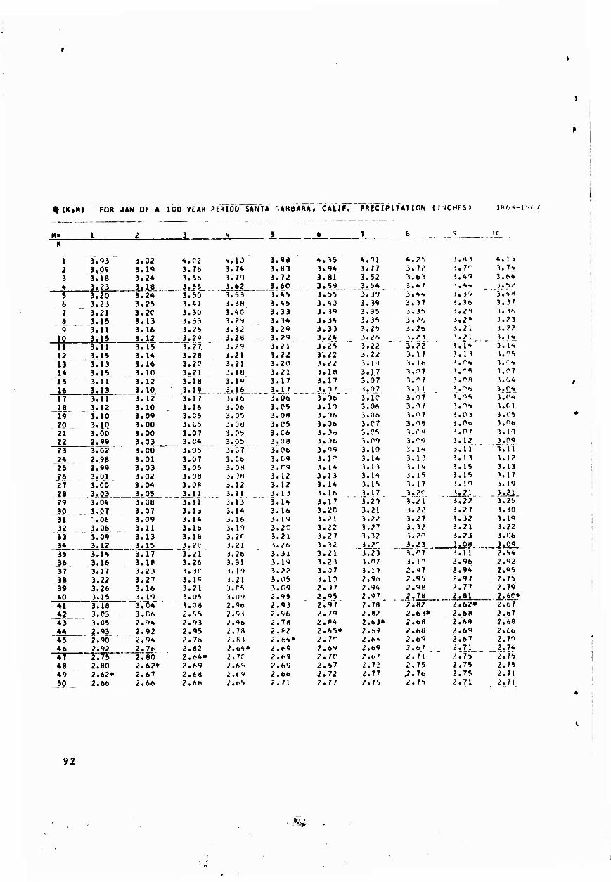
Q(K,N) " FOR JAN OF A ICO VEAH PERIOD SANTA rAKbARA

4 5

, "CALIF7

6

4.35

" PRECmfATlDN

7 8

4.01 4.25

( MCHFSI

3.81

IHfi-

N> 1 2 3 ...1L K

3. « 3.02 4.C2 «..10 3.98 «.13

3.09 3.19 3.76 3.74 3.83 3.94 3.77 3.72 t. rr 3.7«

3.18 3.2« 3.56 3.7') 3.72 3.81 3.52 3.63 i.4i 3.6«

3.23 3.18 3.55 3.62 3.60 3.59 3.54 3.47 <.4H _ J.-.V 3.20 3.2« 3.50' 3.53 3.45 3.55 3.39 3.«.4 J.3 0 3.«H

3.2i 3.25 3.41 3.3H 3.45 3.40 3.39 3.37 1.36 3.3/

3.21 3.2C 3.30 3.40 3.33 3. 39 3.35 3.35 J.2S 3.36

3.15 3.13 3.33 3.2># 3.34 3.34 3.35 3. 70 3.2« 3.23

3.11 3.16 3.25 3.32 3.29 3.33 3.25 3.2b 3.21 J.?2

3.15 3.12 3.29 3.28 3.29 3.24 3.26 3.23 1.21 3.1«

3.11 3.15 3.27. 3.29 3.21 3.25 3.22 3.22" ».1« 3.1«

3.15 3.14 3.28 3.21 3.22 3.22 3.22 3.1/ 3.1 4 3.05

3.13 3.16 3.2C 3.21 3.20 3.22 3.H 3.16 ».^4 1.''4

3.15 3.10 3.21 3.18 3.21 3.1H 3.17 3.!->7 '."•; 3.07

'i5 3.11 3.12 3.18 3.19 3.17 3.17 3.07 3.^7 ^.^a 3.04

3.13 3.10 3.19 3.16 3.17 3.07 3.07 3.11 \.^t> 3.04

3.11 3.12 3.17 3.16 3. 06 3.Ö6 3.10 3.07 >".i«i 3.04

3.12 3.10 3.16 3.06 3.05 3.10 3.06 3.1/ ?.15 3.01

3.10 3.09 3.C5 3.05 3.08 3.06 3.06 3."7 3.03 3.05

3.10 3.00 3.C5 i.06 3.C5 3.06 3.07 3.05 3.0b 3.06

3.00 3.00 3.07 3.05 3.C6 i.Oi 3.r5 -i.r* 1.07 3.n

2.99 3.03 3.C4 3.05 3.08 3. U 3.09 3.^9 3.12 3.09

3.02 3.00 3.05 3.C7 3.06 3.19 3.10 3.14 3.11 ü.ii J?i 2.98 3.01 3.07 3.C6 3.09 3.1•', 3.14 3.13 3.13 3.12

2.99 3.03 3.05 3.OH 3.rq 3.14 3.13 3.1« 3.15 3.13

3.01 3.02 3.08 3.08 3.12 3.13 3.14 3.15 3.15 3.17

3.00 3.04 3.08 3.12 3.12 3.14 3.15 3.17 j.n 3.19

3.03 3.05 3.11 3.11 3.13 3.16 3.17 3.?r ... '•?!_. 3.21

3.04 3.08 3.11 3.13 3.14 3.17 3.20 3.21 1.22 3.25

3,07 3.07 3.U 3.14 3.16 3.20 3.21 i.22 3.27 3.30

-.06 3.09 3.14 3.16 3.19 3.21 3.22 3.27 3.32 3.IQ

3.08 3.11 3.1o 3.19 3.2r 3.22 3.27 3.32 3.21 3.22

3.09 3.13 3.18 3.2r 3.21 3.27 3.32 3.2-1 3.23 3.C6

3.12 _...3.15 3.2C 3.21 3.26 3.32 3.2" 3.23 3.08 3.09

3.14 3.17 3.21 3.26 3.31 3.21 3'. 2 3' 3.07 3.11 2.94

36 3.16 3.IP 3.26 3.31 3.19 3.23 1.07 3.1" 2.96 2.92

3.17 3.23 3.3r 3.19 3.22 3.07 3.n 2.97 2.94 2.95 3.22 3.27 3.1«? i.2l 3.05 4.10 2.9(, 2.^5 2.97 2.75

3.26 3.16 3.21 i.r', 3.09 2.^7 2.'H 2.08 2.77 2.79

3.15 i.19 3.05 3.U9 2.95 2.95 2.97 2.78 2.81 2.60»

3.18 3.o«r 3.08 2.9o 2.93 2".9> 2.78 2.82 2.62« 2.67'

3.03 3.C6 i.'.'i 2.<i3 2.96 2.70 2.«? 2.63* 2.68 2.67

3.05 2.94 2.03 <;.96 2.78 2.P4 2.63* 2.68 2.68 2.68

2.93 2.92 2.95 ^.78 2.^2 2.65* 2.69 2.66 2.6" 2.66

2.90 2.9<, 2.7ö ^.m 2.64» 2.7' 2.6^ 2.69 2.67 2.7" 2.92 2.76 2.82 2.64* 2.65 2.69 2.69 2.6/ 2.71 2.7«

2.75 2.80 2.64» 2.7r 2.69 2.70 2.67 2.71 2:75 2;75

2.80 2.62» 2.^9 i.h^ 2.69 2.b7 2.72 2.75 2.75 2.75

2.62* 2.67 2.68 2.»9 2.66 2.72 2.77 ^.76 2.7«; 2.71

50 2.66 2.66 2.6B i.L'} 2.71 2.77 2.75 2.75 2.71 2.71

92

OMK.HI FUR JAN OF A 100 YfcA« PERIOD SANTA HAKBAHA, CALIF. PP6CIFITAIIDN (INCHFSI IRftS-lOf.?

1" K

50.24 15.25 52.25 55.01 50.73 64. 3 7 52.22 61.65 46.52 59.6-.

16.01 21.63 42.59 41.44 45.06 48.62 43.20 41.75 41.25 43.Oh

21.54 23.62 35.CC 40.17 40.64 44.03 33.84 38.H 33.45 39.fl|> 23.27 21.33 34.66 36.99 36.57 35.65 34.56 32.^3 31.60 35.28

22.26 23.31 32.72 33.46 3C.67 34.07 28."2 30 . 74 20.5? 53.77

23.57 23.62 29.17 26.03 30.85 2H.24 26.93 28.2^ 28.22 29.58

22.72 21.77 25.02 26.67 26.CJ 2H.09 27.23 27.64 >,>.'3n 29.04

20.50 19.16 26.16 24.35 26.51 26.12 27.22 24.2" '5.44 24.28

16.84 20.49 23.22 25.75 24.60 25.67 23.57 24.21 22.56 23.73

20.49 19.00

18.76 20.13

24.66 23.76

24.15 24.40

24.63 21.46

22.17 22.69

24.01 22.32

22.''" 22.47

22. 6 J 20.01

20.81 20. 5-.

20.45 19.56 24.16 21.39 22.08 21.59 22.43 20.76 19.62 17.13

19.75 20.26 21.39 21.65 21.08 21.64 20.8? 2C.3 3 16.07 16.92 20.57 18.29 21.70 20.54 21.61 19.97 20.61 16.«4 16.43 18.06

18.85 16.91 20.56 2C.88 20.2Ü 19.88 16.53 16.86 17.86 16.81 19.65 18.21 21.05

20.10 IS. 74 19.62

19.9«) 15.Hi

15.77 15.66

16.74 17.94

18.2«» 16.99

16.79 16.44

16.7.^ 16.65 18.71 16.83 19.23 17.97 19.63 15.74 15.72 17.12 16.36 16.76 16.50 15.P4 16.60 17.70 15.79 15.60 16.75 15.61 16.55 16.90 15.63 17.07 16.39 14.2» 15.62 16.58 15.4S 15.73 16.63 16.17 16.86 17.58 14.65 14.18 16.53 15.46 15.90 16.15 15.98 17.28 17.26 19.07 14.43 15.33 15.24 15.62

16.27 16.50 15.85

15.42 16.58

17.24 17.62

17.8» 19.44

19.05 18.95

18.87 15.36 14.22 15.52 T'9.3H 14.05 14.61 16.21 15.64 16.94 16.94 19.16 19.04 19.54 19.92 14.45 15.26 15.68 16.67 17.07 18.43 18.90 19.S« 2".22 70.^3

lb.05 14.87 16.67 16.7r 18.25 18.23 19.47 2( ."7 -»O.V' 21.84 14.85 15.91 10. T) 17.97 lb.07 18. 74 l^.Sl 2 i . '> I ?l.i^ ^2.53 15.33 lö.05

17.25 18.Ul 17.34

1 7.8t. It^?

1H.5'' 19. 2r. 20.36 21 .4^

21.7- 22.32

22.5« 23.1 7

23.2'" 16.C2 24.91

17.1b 17.06 l".*»^ i^.tl 19.7'; 2.,.7'. 2 1. 9'' 22.' • 24.8 3 2t..8') 16.93 17.79 It. St. IS.ö' i f • 0 J 21 . .» ' 2<.'.2? 24.4/. 26.71 22.66 17.63 lfl.J4 19.6^ 2':.5., 21.3^ 21.t.4 <?4 . 1 < 26.2" 2^.57 2^.62 16.23 19.11 2C.fc7 21.21 2l.fc< 23. 55 25.95 2c.'- 1 23.55 17.67 19.07 20.14 21. 35 21.'4 ^^,^** 25. <<, 21 .61 22.92 U.'.pl 16.77 20.12 20. an 21.65 23.'•I 25.2^ 21.02 22.63 16.9H 1/1. f.4 13. is 20.66 21.22 23.4'» 25.Its «■cos 21. JIM It. 72 U. 11 13. ^7 12.35 21.22 23.05 25.23 2o.ei 21.hi 15. 7«. 17.B1? 12. 8S 12.24 13.47

36 23.02 24.77 20.65 21. oft Xh.w, 17. J2 12.58 12.14 1 1. 4 .^ 5.82 39 2h.1i 20.55 21. 75 15.54 16.9^ 12. )8 11 .89 13.31 5.73 7.35 >P 20.4'»

21.60 21.47 15.6B

lt.. 75 lt.82

16.74 11.M4

11.40 ll.f '

11. U 12.2"

13.Ol 5.72

5.86 "'n3o"

7.17 Ö.Ö •

0.0 ♦ 2.46 '

15. 7f, 16.6d 11.9H 11.0 * 12.:. 2 5. ■}\ 7.09 p.n * 2.42 2.56 16.63 12. 17 1?.S6 11.84 5.41 7. -V, .-.r • 2.12 2.28 3.05 12.C9 11.16 11.75 5.M Ö.SS r>. ] • 2.n 2.r<' /.M2 2.IP 10.95 11.85 5.27 7.ni r.o ♦ 1. V 1.4t> 2.47 1.67 3.94 11.71 5. 13 C.S6 C.C • 1.98 I .o7 2.38 i .'in 3.5* 5. 4P 4.9ö 6.82 P.C * 2.C2 1.80 1. 15 1.52 3.2« ~" 4.90 5.79

46 6.85 n.o • 1.H2 1.67 1.85 '-.Hr. 3. »5 4.84 5.16 5.72 49 C.C • 1.84 1.46 1.7^ 0.70 2.6^ 5.07 5.^6 •i.oa 4.27 50 1.62 I. W 1.41 r.j« 2.70 4.0' A .^4 4.75 3.41 4.16

93

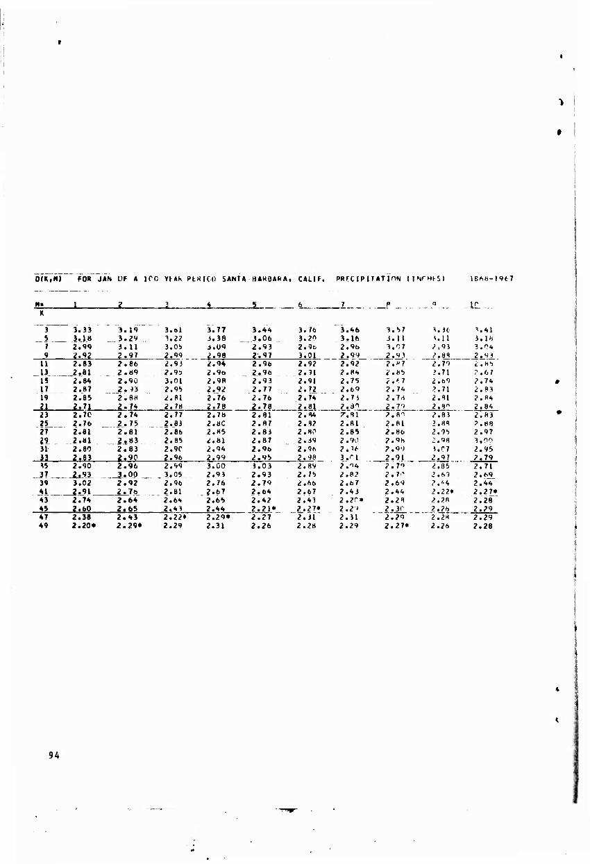
O(KfN) FOR JAN Vf A ICO VUK PtHICO SANTA BAHQABA, CALIf. PRf C IP IT AT ION (INfMI^SI l8iSf3-I9fr7

M« IT

3 3.33 3.19 3.ol 3.77 3.44 3.76 5 3.18 3.29 1.2? 3.38 3.06 3.2" 7 2.99 3.11 3.0!) 3.09 2.93 2.9c 9 2.92 2.97

2.93 2.94 1.91 2.96

3.01 U 2.83 2.66 2.92 13 2.81 2.Ö9 2.95 2.9«, 2.96 2.n 15 2.84 2.90 3.01 2.98 2.93 2.91 17 2.87 ?.« 2.9!) 2.92 2.77 2.72 19 2.85 2.88 2.B1 2.76 2.76 2.74 21 2.71 2.74 2.7« 2.78 2.78 2.81 23 2.7C 2.74 2.77 2.7b 2.81 2.H4 25 2.76 ._-_2.75 . 2.83 2.8C 2.87 2.'?? 27 2.81 2.81 2.86 2.H5 2.83 2.80 29 2.81 2.83 2.85 2.81 2.87 2.39 31 2.80 2.83 2.9C 2.94 2.96 2.96 33 2.83 2.9C 2.96 2.99 2.95 2.98 M 2.90 2.96 2.99 3.00 3.03 2.89

-37 LJA 39 3.02

3.00 2.92

3.05 2.96

2.93 2.76

2.93 2.79

2.75 2.66

Al. 2.91 43 2.74

2.76 2.64

2.81 2.6*

2.67 2.65

2.64 2.42

2.67 2.43

45 2.60 2.65 2.41 2.44 2.21* 2.27 47 2.38 2.43 2.22« 2.29« 2.27 2.31 49 2.20* 2.29« 2.29 2.31 2.26 2.2«

3.46 3.16 2.96

2.92 2.84 2.75 2.69 2.73

r.<u 2.81 2.85 2.90 ?.■>(■ 3.ri 2.14 2.8? 2.67 2.43 2.2^» 2.2* 2.31 2.29

3.57 3.11 3.07

?.H7 2.85 2.'7 2.74 2.7rt

J.'TL ?.fli 2.81 2.86 2.98 2.94 2.91 2.7" 2.7-' 2.61 2.44 2.28 2.3r 2.29 2.21*

^.3t ^.11 2 = 93 1'^ 2.79 -'.71 ^.69 ?.71 2.S1 2.8" 2.83 2.81 2.95 2.^8 3.07 2.97 2.85 2.hi ?.'<, 2.22* 2.2*

'2.28 2.26

3.41 3.lh 3.04

2. hi 2.67 2.74 2.83 2.84 2.84 2.83 ?.«8 2.97 3.00 2.95 2.79 2.71 2.69. 2.44 2.J1» 2.28 2.29 2.29 2.28

94

/

DF(K ,M) FOR JAN Uh A 1 ?C Vf-AK fTRlüO SANTA ÖARHARA, CALIF. PRECIPITATION «INCrtFS» 1868-1967

H» J. 2 .3 4 5 6 7 8 9 IP K

•>1.84 3^.41 62.22 64.45 55.87 65.14 57.12 57.40 51.34 "50.1^ 44.7b 43.77 44.72 47.64 3d.64 40.82 43.85 37.17 40.28 40.11 35.97 3b. 15 37.19 34.9=} 32.92 30.30 34.75 35.72 31.90 33.71 32.89 29.0 7

2'5.8'i 24.^6

34.IÖ 3i.5b

3C.0P 2V.5 1

34.4 3 33.98

32.49 2 8.38'

35.83 '32.69

29.35 26. R5

29.98 28,72 25.63 25.33

27.80 2b.54 32. K ^'^.^■:> 34.16 28.06 29.29 25.7^ 22.17 17.65 29.23 26.85 35.50 3C.0J 32. P 3 27.91 25.02 17.97 20.98 2r.37 30.68 28.25 32.72 27.56 25.33 19.77 22.13 21.06 22.19 24.38 29.88 26.10 26.49 2^.57 24.91 20.48 23.93 22.71 26.54 25.12 23.42 23.01

19.74 19.64

25.00 24.67

21.5-^ 21.33

26.13 27.13

23.49 ^4.9''

27.16 27.92

23.22 23.65

2^.29 24.84 27.42 24.69

25.79 20.15 27.07 22.44 30.07 23.98 27.9R 24.00 29.87 26.65 27.75 22.97 28.36 24.31 28.41 2 3 . 2 < 29.80 26.29 33.13 30.44 27.97 23.57 26.26 22.71 29.9d 26. »" 31.87 31.51 34.28 31.94 27.50 23.66 30.21 2fl.l6 34.21 30. ?" ?4.44 31.92 33.17 29.71 29.02 26.76 32.95

34.20 3C.34

'■3('.83 33.%4 37.44

31. -i 3 27.11

3b.Q3 33.4 7

26.32 23.05

33.69 28.62

22.95 31.89 29.28 I".06 33.56 31.26 37.P9 28.12 32.5b 20. n 2fl.3C 19.09 21.30 lfl.47 37.49 27.66 32.99 2C.bt) 2b.44 16.79 21.41 18.85 9.97 7.34 32.64 20.88 26.33 16.67 I9.fll 17. 17 10.32 7.62 0.0 ♦ 0.0 ♦ 24.91 15.45 18.59 15.51 9.o9 6. 77 0.0 ♦ o.on 2.<'4 0.49 18.31 16.11 9.04 t.b5 0.0 ♦ 0.3 • 4. OH 1.42 1.9S „0i?l_ 8.32 6.14 0.0 ♦ n.c • 2.85 1.44 4.85 1.12 2.58 0.66 0.0 • 0.0 ♦ 3.04 C.75 2.53 C.4<; 4.3;i o.O • 1.91 0.19

95

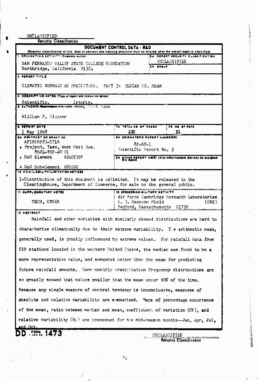
UNCLASSIFIED Sec curlty Cltitlfication

DOCUMINT CONTROL DATA • RIO f$»mirtiy tl»*§llleaUon el mit, bogy el abeincl and mdiKlnt annefiion muel be »n(»f d iWnn the evenll HpoH I» tleeeilied)

I OKIMNATINO ACTlv^" rCotpenle eulhetl

SAN FERNANDO VALLEY STATE COLLEGE FOUNDATION Northridge, California 9132U

la MBPOUT tieuNlTV C LAIIineATION

UNCLASSIFIED lb anoup

i ni^onr TITLI

CLIMATIC NORMALS AS PREDICTORS. PART 3: MEDIAN VS. MEAN

4 DllieillPriVI NOTII (Type el npbrt «itf inelutiv TSu!)

Scientific. Interiri. • A\jrH0n(l)9hm*m»mmJlfei r,»me, lnlilelif 1 ■v-rtTname

William F, Slusser

• NIPORT OATI

1 May 1968 102 31 • • eoNTnACT en SMANT NO

AF19(628)-5716 * Project, Task, Work Unit Mos.

862U-T02-WU 01 ■, DoD Element 62Ü0539F

d DoD Subelement 681000

i)

82-68-1 Scientific Henort No. 3

I* aTHin M'SNT H*(I) f4fl>>«MtrniMittM «itf m«>*kf »«iinti

10 AVAILASIUTV/UMITATION NOTICII

1-Distribution of this document is unlimited. It may be released to the Clearinghouse, Department of Commerce, for sale to the general public.

11 IUI

TECH, OTHER

II IPONIONINO MILITANV ACTIVITV

Air Force Cambridge Research Laboratories L. 3. Kanscom Field (CRE) Bedford, Massachusetts 01730

11 »CT

Rainfall and other variables with similarly skewed distributions are hard to

characterize climatically due to their extreme variability. T. e arithmetic mean,

generally used, is .greatly influenced by extreme values. For rainfall data from

219 stations located in the western United States, the median was found to be a

more representative value, and somewhat better than the mean for predicting

future rainfall amounts. Some monthly orecii itation frequency distributions are

so greatly skewed that values smaller than the mean occur 90^ of the time.

Because any single measure of central tendency is inconclusive, measures of

absolute and relative variability are summarized. Maps of percentage occurrence

of the mean, ratio between median and mean, coefficient, of variation (CV), and

relative variability (Vq ) are presented for the mid-season months—Jan, Apr, Jul, anH Offt..

DD Mi'.. 1473 UNCLASSIFIED flefurity ^läsilFTfaBen

v:

ÜMCUSSIPIH) Security Classification

14 KEY WORDS

MORMALS, CUMATIC

PREDICTION, CLIMATIC

OPTIMUM RECORD LENQIH

HEDUN

LINK A

«OLE WT

LINK B

"OLE WT

LINK C

ROLE WT

INSTRUCTIONS

1. ORIGINATING ACTIVITY: Enter (he name end »ddre«» ot the contractor, subcontractor, grantee, Department of De- fense activity or other organization (corporate author) iaaulng the repjrl.

2a. REPORT SECURITY CLASSIFICATION: Enter the over- all security classification of the report. Indicate whether "Restricted Data" is included. Marking is to be in accord- ance with appropriate security regulations.

2h. GROUP: Automatic downgrading it specified in OoD Di- rective 5200.10 and Armed Forces Industrial Manual. Enter the «roup number. Also, when applicable, show that optional markings have been used for Group 3 and Group 4 as author- ized.

3. REPORT TITLE: Enter the coriplete report title in all capital letters. Titles in all cases should be unclassified. If a meaningful title cannot be selected without classifica- tion, show title classification in all capitals in parenthesis immcriialely following iius title.

4. DESCRIPTIVE NOTES: If appropriate, enter the type of report, e»B., interim, progress, summary, annual, or final. Give the inclusive dates when a specific reporting period is rove.ed.

5. AUTHOK(S): Enter the name(s) of authoKs) as shown on or in the report. Entei last name, first name, middle initial. It Tilitary. show rank »ni branch of service. The name of the prmripal > <thor is an absolute minimum requirement.

h. RFPOR'f DAT^; Enter the date of the report as day, month, year; or month, year. If more than one date appears nn the report, use date of publication.

7a. TOTAL NUMBER OF PAGES: The total page count should follow normal pagination procedures, i.e., enter the number of pages containing information.

7b. NUMBER OF REFERENCES: Enter the total number of references cited in the report.

8a. CONTRACT OR GRANT NUMBER: If appropriate, enter the applicable number of the contract or grant under which the report was written.

8b, He, tb id. PROJECT NUMBER: Enter the appropriate military department identification, such as project number, subproject number, system numbers, task number, etc.

9a. ORIGINATOR'S REPORT NUMBER(S): Enter the offi- cial report number by which the document will be identified and controlled by the originating activity. This number must be unique to this report.

9b. OTHER REPORT NUMBER(S): If the report has been assigned any other repcrt numbers (either by (he originator or by the sponsor), also enter this number(s),

10, AVAILABILITY/LIMITATION NOTICES: Enter any lim- ■ijtions .in furlhcr dissemination of the report, other than those

imposed by security classification, using standard statements such as:

(t) "Qualified requesters may obtain copies of this report from DDC"

(2) "Foreign announcement and dissemination of this report by DDC is not authorized."

(3) "U. S. Government agencies msy obtsin copies of this report directly from DDC. Other qualified DDC users shall request through

(4) **U. S. mililary agencies may obtain copies of this report directly from DDC Other qualified users shall request through

(i>) "All distribution of this report is controlled Qual- ified DDC users shall request through

if

If the report has been furnished to the Office of Technical Services, Department of Commerce, for sale to the public, indi- cate this fsct and enter the price, if known.

11. SUPPLEMENTARY NOTES: Use for sdditional explana- tory notes.

12. SPONSORING MILITARY ACTIVITY: Enter the name of the departmental project office or laboratory sponsoring (pay ing for) the research and development. Include address.

13 ABSTRACT Enter an abstract givinj ° brief and factual summary of the document indicative of the report, even though it may also appear elsewhere in the body of the technical re- port. If additional space is required, a continuation sheet shall be attached.

It is highly desirable that the abstract of classified reports be unclassified Each paragraph of the abstract shall end with an indication of the military security classification of the in- formation in the paragraph, represented as rrs;. rs;. (C). or (V)

There is no limitation on the length of the abstract. How- ever, the suggested I'-ngth is from 150 to 225 words.

14. KEY WORDS: Key words are technically meaningful terms or short phrsses that characterize a report and msy be used as index entries fur cataloging the report. Key words must be selected so that no security classification is required. Identi- fiers, such as equipment model designation, trade name, military project code name, geographic location, may be used as key words but will be followed by an indication of technical con- text. The assignment of links, rules, and weights is optional.

iiMnngaTCTgn Security Classification

Ifw-' ■■ '

r .1 SAN FERNANDO VALLEY STATE COLLEGE

NORTHR1DGE, CALIFORNIA

11 September 1968

ERRATA SHEET FOR

CLIMATIC NORMALS AS PREDICTORS

Part 1: Background AFCRL 67-0313 - ^ V 3 <

T2 Part 3: Median vs. Mean AFCRL-68-0255 - ^ ''

In Part 1, distributed In June 1967, the contract number

on the cover should be corrected to read:

AF19 (628) - 5716

In Part 3, distributed in July 1968, In Form DD 1473 (the

final page of report), block 9b should contain the number,

which also appears on the cover:

AFCRL-68-0255

q

In Part 3 also, page 81, entitled "Climatic Prediction,"

should be marked as the start of

APPENDIX II

Part 2 and 4 are in preparation, and will receive the same

distribution as the first two reports.

Arnold Court Principal Investigator

Reproduced by the CLEARINGHOUSE

for Federal Scientific & Technical Information Springfield Va 22151