Eco-climatic assessment of

the potential establishment

of exotic insects in New Zealand

A thesis

submitted in partial fulfillment

of the requirements for the Degree of

Doctor of Philosophy at Lincoln University

by

Lora Peacock

Lincoln University 2005

Abstract of a thesis submitted in partial fulfillment of the requirements for the Degree of PhD

Eco-climatic assessment of the potential establishment of exotic insects

in New Zealand

Lora Peacock

Contents

To refine our knowledge and to adequately test hypotheses concerning theoretical and

applied aspects of invasion biology, successful and unsuccessful invaders should be

compared. This study investigated insect establishment patterns by comparing the climatic

preferences and biological attributes of two groups of polyphagous insect species that are

constantly intercepted at New Zealand's border. One group of species is established in

New Zealand (n = 15), the other group comprised species that are not established (n = 21).

In the present study the two groups were considered to represent successful and

unsuccessful invaders.

To provide background for interpretation of results of the comparative analysis, global

areas that are climatically analogous to sites in New Zealand were identified by an eco­

climatic assessment model, CLIMEX, to determine possible sources of insect pest

invasion. It was found that south east Australia is one of the regions that are climatically

very similar to New Zealand. Furthermore, New Zealand shares 90% of its insect pest

species with that region. South east Australia has close trade and tourism links with New

Zealand and because of its proximity a new incursion in that analogous climate should alert

biosecurity authorities in New Zealand. Other regions in western Europe and the east coast

of the United States are also climatically similar and share a high proportion of pest species

with New Zealand.

Principal component analysis was used to investigate patterns in insect global distributions

of the two groups of species in relation to climate. Climate variables were reduced to

temperature and moisture based principal components defining four climate regions, that

were identified in the present study as, warm/dry, warm/wet, cool/dry and COOl/moist.

Most of the insect species established in New Zealand had a wide distribution in all four

climate regions defined by the principal components and their global distributions

overlapped into the cool/moist, temperate climate where all the New Zealand sites belong.

ii

Contents

The insect species that have not established in New Zealand had narrow distributions

within the warm/wet, tropical climates.

Discriminant analysis was then used to identify which climate variables best discriminate

between species presence/absence at a site in relation to climate. The discriminant analysis

classified the presence and absence of most insect species significantly better than chance.

Late spring and early summer temperatures correctly classified a high proportion of sites

where many insect species were present. Soil moisture and winter rainfall were less

effective discriminating the presence of the insect species studied here.

Biological attributes were compared between the two groups of species. It was found that

the species established in New Zealand had a significantly wider host plant range than

species that have not established. The lower developmental threshold temperature was on

average, 4°C lower for established species compared with non-established species. These

data suggest that species that establish well in New Zealand have a wide host range and

can tolerate lower temperatures compared with those that have not established. No firm

conclusions could be drawn about the importance of propagule pressure, body size,

fecundity or phylogeny for successful establishment because data availability constrained

sample sizes and the data were highly variable.

The predictive capacity of a new tool that has potential for eco-climatic assessment, the

artificial neural network (ANN), was compared with other well used models. Using

climate variables as predictors, artificial neural network predictions were compared with

binary logistic regression and CLIMEX. Using bootstrapping, artificial neural networks

predicted insect presence and absence significantly better than the binary logistic

regression model. When model prediction success was assessed by the kappa statistic

there were also significant differences in prediction performance between the two groups

of study insects. For established species, the models were able to provide predictions that

were in moderate agreement with the observed data. For non-established species, model

predictions were on average only slightly better than chance. The predictions of CLIMEX

and artificial neural networks when given novel data, were difficult to compare because

both models have different theoretical bases and different climate databases. However, it

is clear that both models have potential to give insights into invasive species distributions.

111

Contents

Finally the results of the studies in this thesis were drawn together to provide a framework

for a prototype pest risk assessment decision support system. Future research is needed to

refine the analyses and models that are the components of this system.

Keywords: analogous climates, artificial neural networks, CLIMEX, discriminant

analysis, establishment success, host plant, invasive species, kappa statistic, pest risk

analysis, polyphagous insect pest species, principal component analysis.

IV

Contents

Abstract

Contents

Tables

- ii

-------v - ix

Figures - xi

Chapter 1 Invasion Biology - - - - - 1

1.1 Invasive insects in New Zealand - - - - 1

1.2 Current theory in invasion biology - - - - - - - 3

1.2.1 Terminology - - - - - 3

1.2.2 The invasion process in plants and animals - - - 4

1.2.3 The types of conditions conducive for invasion - 6

1.2.4 The life history characteristics or strategies of invasive -

organisms - - - - - - - - - - - - - - - - 9.

1.2.5 Susceptibility of ecosystems to invasion - - - - - - 11

1.3. The role of climate in species distribution - - - - - - 14

1.3.1 Climate matching - - - - - - - - - - - 14

1.3.2 Current eco-climatic assessment methods

1.4 Objectives of this study - - - - - - - - - -

Chapter 2. The insect and climate databases

2.1. Introduction - -

2.2. Methods - - -

2.3. Results and Discussion -

- 16

- 22

- 25

- 25

- - - 25

- - - - - 33

Chapter 3. The Role of Analogous climates in the assessment of invasion success

and establishment of insect pests

3.1 Introduction - -

3.2 Method

3.3 Results

3.4 Discussion-

- - - - 46

- 46

- 48

- 50

- - - 53

Contents

v

Contents

Chapter 4. Principal component analysis: a useful tool in defining global

insect pest distribution - - - - - - - - - 55

4.1 Introduction

4.2 Method -

4.3 Results -

4.4 Discussion -

- - - - - - - - 55

- - - 56

- - 56

- - 64

Chapter 5. Climate variables and their role in site discrimination of polyphagous

insect species distributions - - - - - - - - 68

5.1 Introduction - - - - - - - - - - - - - 68

5.2 Method - - - - - - - - - - - - - 70

5.3 Results and Discussion - - - - 71

Chapter 6. The application of artificial neural networks to insect

pest prediction -

6.1 Introduction

6.2 Method - - - -

- - - - 81

- - - - - 81

- - - - - 84

6.2.1 Modelling approach - - - - - - - - - - 87

6.3 Results - - - - - 89

6.4 Discussion - 96

Chapter 7. Biological factors that may assist establishment of insect

pests in New Zealand - - - - - - - - - - - 101

7.1 Introduction

7.2 Method - -

7.3 Results and Discussion

7.3.1 Host plant range -

101

- - 101

- - - - - 103

7.3.2 Developmental requirements - - -

103

104

106

108

111

7.3.3. Propagule pressure and body size -

7.4 Taxonomic differences - - - - - - - -

7.5 Combining biological and climate variables

vi

Con/elliS

Chapter 8. Comparison of the prediction of insect establishment into New

Zealand by artificial neural networks and CLIMEX - - - 115

8.1 Introduction - - - - - - - - - - - 115

8.2 Methods - - - - - - - - - - - - 116

8.3 Results - 118

The yellow scale, Aonidiella citrina - - - - - - 118

The coconut scale, Aspidiotus destructor - - - 121

Palm thrips, Thrips palmi - - - - - 124

The western flower thrips Frankliniella occidentalis 127

The light brown apple moth, Epiphyas postvittana - - - 130

Onion thrips, Thrips tabaci

8,4 Discussion - - - - - - - - - -

Chapter 9. General Discussion

9.1 Pest risk analysis - '. - - -

9.2 Pest risk analysis in New Zealand

9.2.1 Pest risk analysis in New Zealand -

9.3 Combining multivariate and modelling techniques to assess

pest establishment - - - - - - - - -

9,4 Testing the prototype method - - - - -

9.5 Conclusions and future progress - -

Chapter 10. References -

133

137

- - - 139

139

- 141

- - - 138

142

- 149

151

153

Chapter 11. Appendices - - - - - - - - - - - - - - - - - - - 184

Appendix I List of all polyphagous insect species that have been intercepted in

New Zealand 184

Appendix II Current global distributions of the study species - - - - - - 188

Appendix III Table of analogous climatic regions to Auckland based on the

CLIMEX match function - - - - - - - - - - - - - - - - - - - 198

Vll

COn/ellis

Appendix IV. Proportion of sites where insects species have been correctly

classified absent by the discriminant function for each climate variable- - - - 205

Acknowledgements - - - - - - - - - - - - - - - - - - - - 208

viii

Contents

Tables

Chapter 2

Table 2.1 A description of the climate parameters used in this study - - - - 31

Table 2.2. Country of origin and interception rate of polyphagous insects per year and

Table 2.3.

Table 2.4

Table 2.5.

per metric tonne of imported plant produce (1993-1999) 34

The global distribution of the insects sampled for further study 38

The number of host plant species and plant families recorded for each

species - - - - - - - - - - - - - - - - - - - 40

Adult body length (mm), fecundity rate and reproductive strategy for each

species .. - - - - -- - - - - - - - - - - - - - - - - 42

Table 2.6. The lower developmental threshold eC) and developmental time (in degree

days (OC) for each species - - - - - - - - - - - - - - 45

Chapter 3

Table: 3.1. Percentage of insect species identified from CABI distribution maps (1961-

1996) recorded as occurring in each of the analogous climate regions 52

Chapter 4

Table: 4.1. The coefficients of the first and second principal component loadings

(weights) for each climate variable and alongside the calculated correlation

coefficients (r) - - - - - - - - - - - - - - - - - - 58

Chapter 5

Table 5.1. Z values for insect pest species established in New Zealand - - - 73

Table: 5.2. Z values for insect pest species non-established in New Zealand - - 74

ix

Table: 5.3.

Table: 5.4.

Chapter 6

Table 6.1.

Table 6.2.

Chapter 7

Table: 7.1.

Chapter 9

Table: 9.1

Contents

Proportion of sites where insects species already established in New

Zealand have been correctly classified present by the discriminant function

for each climate variable - - - - - - - - - - - - - - - 75

Proportion of sites where insect species not yet established in New Zealand

have been correctly classified present by the discriminant function for each

climate variable - - - - - - - - - - - - - - - - - - 76

Indicators for assessing prediction success of absence/presence

models - - - - - - - - - - - - - - - - - - - - - 88

Mann-Whitney test of mean model performance for each Insect pest species

over the iterated validation datasets - - - - - - - - - - - 92

The coefficients of the first and second principle component loadings

(weights) for each variable with the corresponding correlation

coefficient (r) - - - - - - - - - - - - - - - - - - 111

Summary of the results from the protype decision support methodology

illustrated in Figure 9.1 for assessing the establishment of polyphagous

insect species arriving in New Zealand - - - - - - - - - - 150

x

Contents

Figures

Chapter 2 Figure 2.1. The mean number of CABI publications for the sub-sample and the larger

Figure 2.2.

Figure 2.3.

Chapter 3

un-sampled population of intercepted insect species - - - - - - 28

Linear regression of annual insect interception rate versus plant import

volumes - - - - - - - - - - - - - - - - - - - - 35

Linear regression of annual insect interception rate versus distance (km)

From source of plant import ants - - - - - - - - - - - - 35

Figure 3.1. Map showing analogous climatic regions to Auckland, New Zealand (A)

(lat: 36.80° S, long: 174.80° E) based on the CLIMEX match function 51

Chapter 4

Figure: 4.1 Classification of the climates derived from the principal components 59

Figure: 4.2 Principal component plots of the global distribution of each insect pest

(n=15) that are already established in New Zealand - - - - - - 61

Figure: 4.3. Principal component score plot of the New Zealand climate sites - 62

Figure: 4.4 Principal component scores of the global distribution of insect species

(n=21) not established in New Zealand - - - - - - - - - - 64

Chapter 6

Figure 6.1. Depiction of a multi-layer feed-forward neural network architecture 86

Figure 6.2. Artificial neural network (ANN), and Binary logistic regression (BRM)

mean performance for each insect pest species - - - - - - - - 91

xi

Contents

Figure 6.3. Artificial neural network (ANN), and Binary logistic regression (BRM)

mean kappa statistic for each insect pest species - - - - - - - 95

Figure 6.4. Artificial neural network (ANN), and Binary logistic regression (BRM)

mean kappa statistic for the group of insect pests that have already

established in New Zealand (white) and the group of insect pests that have

not yet established (grey) - - - - - - - - - - - - - - - 95

Chapter 7

Figure 7.1. Mean plant host insect occurrence from CABl database search

(1972-2000) - - - - - - - - - - - - - - - - - - - 103

Figure 7.2 Mean lower developmental thresholds ( C) for groups of insect pest species

that have not yet established (n = 8) and those that have (n = 10), gathered

. from literature (see table 2.6 for data) - - - - - - - - - - 105

Figure 7.3 Mean developmental time for groups of insect pest species that have not yet

established (n=6) and those that have established (n=lO), gathered from

literature (see table 2.6) - - - - - - - - - - - - - - - 105

Figure 7.4 Mean annual intercept rate from MAF interception data (1993-1999) for

groups of insects that have not yet established (n = 114) and those that have

(n = 18) - - - - - - - - - - - - - - - - - - - - 107

Figure 7.5. Number of species in each taxonomic family that have either established or

failed to successfully establish in New Zealand (from the interception data

1993-1999) - - - - - - - - - - - - - - - - - - - 109

Figure: 7.6 Principal component score plots of the climate and biological variables for

each insect pest species (n = 14) - - - - - - - - - - - - 113

xii

Coli/ellis

Chapter 8

Figure 8.1. Observed distribution (a) of the yellow scale, Aonidiella citrina derived

from literature search (Table 2.4). (b) Predictions made by artificial neural

network (ANN). Output is an establishment index (0-100) and (c) is

the eco-c1imatic index (0-100) or suitability of each site for establishment

by CLIMEX - - - - - - - - - - - - - - - - - - - 119

Figure 8.2. Predicted establishment of yellow scale, Aonidiella citrin a in New Zealand

using novel meteorological data at 281 sites. (a) Artificial neural network

gives an index of establishment at each site and (b) CLIMEX predicts the

suitability of a site for establishment using an eco-c1imatic index - 120

Figure 8.3. Observed distribution (a) ofthe coconut scale,Aspidiotus'destructor

derived from literature search (Table 2.4). (b) Predictions made by

artificial neural network (ANN). Output is an establishment index

(0-100) and (c) is the eco-c1imatic index (0-100) or suitability of each site

for establishment by CLIMEX - - - - - - - - - - - - - 122

Figure 8.4. Predicted establishment of the coconut scale, Aspidiotus destructor in

New Zealand using novel meteorological data from 281 sites. (a)

Artificial neural network gives an index of establishment at each site

and (b) CLIMEX predicts the suitability of a site for establishment

using an eco-c1imatic index - - - - - - - - - - - - - - 123

Figure 8.5. Observed distribution (a) of the palm thrip, Thrips palmi,

derived from literature search (Table 2.4). Predictions made by (b)

artificial neural network (ANN). Output is an establishment index

(0-100) and (c) is the eco-c1imatic index (0-100) or suitability of each site

for establishment by CLIMEX - - - - - - - - - - - - - 124

X111

Contents

Figure 8.6. Predicted establishment of palm trips, Trips palmi in New Zealand

using novel meteorological data at 281 sites. (a) Artificial neural network

gives an index of establishment at each site and (b) CLIMEX

predicts the suitability of a site for establishment using an

eco-climatic index - - - - - - - - - - - - - - - - - 126

Figure 8.7. Observed distribution (a) of the western flower thrips Frankliniella

occidentalis derived from literature search (Table 2.4). (b) Predictions

made by artificial neural network (ANN). Output is an

establishment index (0-100) and (c) is the eco-climatic index (0-100)

or suitability of each site for establishment by CLIMEX 128

Figure 8.8. Predicted establishment of the western flower thrips Frankliniella

occidentaiis in New Zealand using novel meteorological data at

281 sites. (a) Artificial neural network gives an index of establishment

at each site and (b) CLIMEX predicts the suitability of a site for

establishment using an eco-climatic index - - - - - - - - - 129

Figure 8.9. Observed distribution (a) of the light brown apple moth, Epiphyas

postvittana derived from literature search (Table 2.4). (b) Predictions

made by artificial neural network (ANN). Output is an establishment

index (0-100) and (c) is the eco-climatic index (0-100) or suitability of

each site for establishment by CLIMEX - - - - - - - - - - 131

Figure 8.10. Predicted establishment of the light brown apple moth, Epiphyas

postvittana in New Zealand using novel meteorological data at

281 sites. (a) Artificial neural network gives an index of establishment

at each site and (b) CLIMEX predicts the suitability of a site

for establishment using an eco-climatic index - - - 132

XIV

COlllenls

Figure 8.11. Observed distribution (a) of onion thrips, Thrips tabaci derived

from literature search (Table 2.4). (b) Predictions made by artificial

neural network (ANN). Output is an establishment index (0-100)

and (c) is the eco-climatic index (0-100) or suitability of each site for

establishment by CLIMEX - - - - - - - - - - - - - - 134

Figure 8.12. Predicted establishment of onion thrips, Thrips tabaci in New Zealand

using novel meteorological data at 281 sites. (a)Artificial neural network

gives an index of establishment at each site and (b) CLIMEX predicts

the suitability of a site for establishment using an eco-climatic index 135

Figure 8.13. Ilustrated non-established insect pests are: (a) yellow scale Aonidiella

citrina, (b) the coconut scale, Aspidiotus destructor, (c) palm thrips, Thrips

palmi. Established insects are the (d) western flower thrips, Frankliniella

occidentatis, (e) light brown apple moth, Epiphyas postvittana, and (f)

the onion thrip, Thrips tabaci - - - - - - - - - - - - - 136

Chapter 9

Figure: 9.1 Prototype decision support methodology for assessing the establishment

of polyphagous insect species arriving in New Zealand - - - - - 143

xv

1: Invasion biology

1. Invasion Biology.

1.1 Invasive insects in New Zealand

New Zealand is located in the Pacific Ocean and spans a latitude of 34-4rS and longitude

166 - 178°E. New Zealand was historically free of serious insect pest problems until the

arrival of the Polynesian, approximately 1000 years ago. Robust species such as fleas, lice

and scabies mites survived the long distance journey from the islands of Polynesia by

parasitising their human and animal hosts (Cook et al. 2002). Seven hundred years later,

colonists arrived from the United Kingdom and Western Europe bringing more exotic

insect species to New Zealand. Initially, many of these arthropod species were associated

with domestic farm animals, for example, sheep blowfly, Lucilia sericata (Meigen), but

when extensive transformation of the natural environment into large-scale pastoralism and

horticulture began, the introduction of phytophagous insect species escaiated (Hackwell &

Bertram 1999). Many of these species established easily as their required host plants were

the exotic flora that the European had already introduced. For example, the cabbage aphid,

Brevicoryne brassicae (Linnaeus), was recorded in the 1860s, shortly after the introduction

of cruciferous plants (Cook et al. 2002). Initially, the source of these new insect species

was limited, with most originating from Western Europe. However, after the expansion of

global trade and tourism in the latter half of the 20th century, the origin of insect species

new to New Zealand became more varied, with arrivals originating from many places,

including tropical and subtropical areas such as Asia. According to the Ministry of

Agriculture and Fisheries (MAF), from 1996-99 there were two successful establishments

of herbivorous insects per year (Barlow & Goldson 2002).

Agriculture and horticultural products are important components of New Zealand's export

earnings and much effort goes into minimising the impacts of invertebrate pests on these

industries. The direct economic cost to New Zealand caused by invertebrate plant pests

has been estimated to be at least $NZ880 million per year, including costs associated with

losses in agricultural output and expenses associated with eradication or control

programmes to reduce pest impacts (Barlow & Goldson 2002). Examples of some

introduced insect pests in New Zealand that cause significant economic losses are:

argentine stem weevil, Listronotus bonariensis (Kuschel), the weevil, Sitona discoideus

Gyllenhal, blue-green lucerne aphid, Acyrthosiphon kondoi Shinji, black beetle,

Heteronychus arator (Fabricus), the Tasmanian grass grub, Acrossidius tasmaniae (Hope),

1

1: Invasion biology

codling moth, Cydia pomonella (Linnaeus) and the light brown apple moth, Epiphyas

postvittana (Walker).

Once established, exotic insect species can also cause ecological adverse effects on the

indigenous flora and fauna. For example, the common wasp, Vespula vulgaris (Linnaeus),

has penetrated native New Zealand beech (Nothofagus spp.) forest altering the natural food

web by competing with native birds for honeydew, the nectar produced by the sooty beech

scale, Ultracoelostoma assimile (Maskell) (Kay 2002). Also, some native vegetation types

are susceptible to defoliation from polyphagous species such as the painted apple moth,

Teia anartoides (Walker) (Barlow & Goldson 2002, Kay 2002). Unfortunately, details

about impacts on native invertebrates, for example, the parasitism of native scarab beetles

by the scoliid wasp Radumeris tasmaniensis Saussure, are limited, partly because more

emphasis is placed on quantifying and reducing insect pest impacts on agricultural and

horticultural systems.

The likelihood of increases in the incidence of arboviruses that are vectored by exotic

insects and that may affect humans has become a major concern for health services in New

Zealand. For example, the southern saltmarsh mosquito, Ochlerotatus (Ochlerotatus)

camptorhynchus (Thomson), a carrier of Ross River virus, found established in Napier in

1998, has subsequently spread throughout the North Island and has now reached

Marlborough in the South Island (2004). Many other mosquito species are continually

intercepted at the border (Cook et al. 2002, Brady, 2002). Other potential insects that pose

a threat to human health include some ant species, for example, a nest of red imported fire

ants, Solenopsis invicta Buren, were detected and eradicated near Auckland International

airport in 2001 (Brady 2002). The red imported fire ant has still not managed to establish,

despite its frequent incursions at the border.

New Zealand has developed stringent biosecurity strategies to prevent insect pest species

from establishing and causing further economic and ecological damage. But despite this

rigorous system some insects still establish, even under the most adverse environmental

conditions (Simberloff 1989, Barlow & Goldson 2002). It is possible that even just one or

two individuals that have been missed at the border could establish (Memmott et al. 1998,

Grevstad 1999). Whilst there is considerable information in the invasion biology literature

on invasive weeds, invasive fish, introduced birds and mammals, there is often a lack of

2

1: Invasion biology

critical information on the mechanisms that drive the establishment process of insects or

enable certain insect species to be more successful invaders than others. Insects are

distinct in that they have complex physiological life cycles governed greatly by

environmental cues (Messenger 1976). It may be that an insect's response to

environmental conditions are more important in determining establishment success than

biological or biotic factors. In other words, this thesis attempts to determine which aspects

of current invasion theory are applicable to invasive insect species.

1.2 Current theory in invasion biology

1.2.1 Terminology

The terminology 'invasive species' is commonly used throughout the invasion biology

literature to describe a species that has successfully established and extepded its range in a

new area (Duncan et al. 2003a, Kolar & Lodge 2001, Richardson et al. 2000, Williamson

1996). However, there are many other adjectives that have been used to describe invasive

species. For example, 'alien', 'pest', 'exotic' and 'introduced' are often used instead of

'invasive'. Variation in terminology can lead to confusion especially if specific definitions

are required, particularly in pest risk management that relies on scientific knowledge to

determine the likelihood of insect species establishment and their potential impacts on the

environment (Davis & Thompson 2000). Consistent terminology would help those,

particularly in biosecurity, who need to know whether newly established insect species will

be harmful to human health, agricultural/horticultural production and or indigenous

ecosystems. For instance, 'pest' or 'weed' implies that the species is likely to compete

with humans for the same agricultural and horticultural resources (Bazzaz 1986), including

native species, for example the native beetle, Costelyta zelandica (White), is a serious pest

of pasture in New Zealand.

However, there is more agreement in the literature with the definition of 'establishment' of

a species. Duncan et al. (2003b), Kolar & Lodge (2001), Richardson et al. (2000),

Vermeij (1996) Williamson (1996), Williamson & Fitter (1996a) all agree that an

established species is a self-sustaining population, outside its natural range.

The expression 'invasive alien species' possibly appeared in the literature sometime in the

1980s. This somewhat emotive expression seems more useful to capture he attention of

3

1: Invasion biology

the appropriate funding authority. While this statement may seem somewhat cynical the

phrase does capture the imagination of the general public and can alert individuals to the

threat posed by such species.

1.2.2 The invasion process in plants and animals

The effects of invasive organisms on native species communities has long been recognised

(Elton 1958, Lodge 1993). However, many initial studies have been carried out on well

established species that had invaded the new area many years ago. A good example, is the

deliberate global introductions of the European starling, Sturnus vulgaris Linnaeus. This

species has aggressively displaced native species from their nests and competed with them

for food resources in many areas (Elton 1958). Other examples are the intentional

establishment of the North American muskrat, Ondatra zibethica (Linnaeus), into most of

Europe (Elton 1958, Di Castri 1989) where it disturbs natural wetland vegetation patterns

through grazing, burrowing and lodge construction (Connors et al. 2000), and the

Meditteranean pine, Pinus pinaster Aiton, which has replaced much of the native flora in

South Mrica (Di Castri 1989, Heywood 1989). A more recent example of an invasive

species impacting a native species is the zebra mussel, Dreissenia polymorpha (Pallas),

accidentally introduced into the United States from contaminated ballast water in the mid

1980s (Kolar & Lodge 2001). This filter feeder attaches itself to native mussels and

interferes with their feeding and physiology and has been responsible for their decline in

many water-ways in North America, including the Great lakes. Since the number of global

invasive species have increased dramatically causing both worldwide economic and

ecological damage (IUCN 1999), research has become more focused on mechanisms that

drive the invasion process.

The invasion process for a species has been categorised into three clearly defined phases:

1) introduction or arrival, 2) establishment, and 3) spread (Williamson & Fitter 1996a,

1996b, Vermeij 1996, Richardson et al. 2000, Davis & Thomson 2000, Kolar & Lodge

2001, Sakai et al. 2001, Shea & Chesson 2002, Duncan et al. 2003a, 2003b). Phase one, is

the transport of an organism to a new area either through human-derived opportunities or

simply through natural spread (Di Castri 1989).

4

1: Invasion biology

Because the opportunities for arrival on imported fresh plant produce can be considered to

be always present, this study is concerned with stage two of the invasion process with

particular reference to polyphagous insect species. However, the reasons why some insect

species manage to establish self-sustaining populations on arrival or why some species fail

to persist is difficult to predict. Unlike plants and larger animals, insects can be very

difficult to detect in the field and self-sustaining populations of phytophagous insects are

usually first noticed through their impacts on the surrounding flora within the area of

establishment. By this stage it can be often be too late for eradication. Phase three of the

process refers to the established population increasing in size and spreading from its point

of establishment (Duncan et al. 2003a).

Whilst the invasion process may be clearly defined, the mechanisms that allow some

species and not others to succeed remain elusive. Despite that, knowledge of the

mechanisms driving invasion are inconclusive, statistical generalisations have been made

about the proportions of species that will succeed at each stage of the invasion process.

For example Lonsdale's (1994) survey on the fate of introduced exotic pasture species into

Northern Australia between 1947 and 1985 found that 13% became listed as invasive

weeds whilst only 5% were of use for increasing pastoral productivity. Also the tens rule

proposed by Williamson (Williamson 1993, Williamson 1996, Williamson & Fitter 1996a,

1996b) has been used to determine the proportion of invasions succeeding at each stage.

Williamson and Fitter (1996a) suggest that of species that arrive at a new destination, 10%

will establish. Of those that establish, 10% will spread to become pests or weeds. The

authors do point out that the tens rule needs to be interpreted with caution, where 10% is an

estimate between 5 and 20% to take into account uncertainty relating to sampling error or

lack of consensus in the literature on what constitutes an invasive species. Despite the

uncertainty, the rule has loosely fitted data on British angiosperms and British Pinaceae

(pine) (Williamson 1996, Williamson & Fitter 1996a), and Australian pasture plants

(Lonsdale 1994). The rule has also been shown to fit terrestrial/aquatic vertebrates and

arthropods that have managed to become highly invasive in the United States (United

States, Office of Technology Assessment 1983) and the introduction and establishment of

Passeriformes (song-birds) and Columbiformes (doves and pigeons) into Hawaii (Moulton

& Pimm 1986).

5

1: Invasion biology

Like many statistical generalisations, there are exceptions, particularly with insects used in

biological control. Williamson (1996) found that the establishment rate of biocontrol

agents, around 30% was much higher than the tens rule. Williamson suggests that this is

not surprising as such insects are specifically selected to be successful which is reflected in

their high introduction efforts. A preliminary examination by Worner (2002) of some

intensive surveys carried out by Kuschel (1990) and Peck et al. (1998) suggests that the

tens rule may also not apply to insect invasions. Clearly, any explanation of possible

mechanisms that may explain the tens rule is limited as there is no clear understanding of

why certain proportions of some species establish and become invasive but others fail at

different stages of the invasion process (Williamson & Fitter 1996a). The tens rule

predicts that the vast majority of species will fail to establish; however, it is easier to

observe the mechanisms behind successful introductions than ones that fail because

failures tend to be less well documented within the literature (Simberloff1989, Williamson

1996). As well, establishment success or failure is harder to interpret when deliberate

introduction of the target species fails and the introduction effort is increased until there is

a successful result. For example, the European red deer, Cervus elaphus Linnaeus, only

became well established in New Zealand after 31 previous introductions (Sax & Brown

2000) and the European starling, Sturnus vulgaris became widely established in North

America after 8 previous attempts at introduction (Elton 1958, Di Castri 1989). Even so,

what makes any species invasive is still contentious, but the general consensus is that to

explain species invasion, the following factors need to be considered: 1) the types of

conditions conducive for invasion, 2) the characteristics or life strategies that predispose an

organism to invade and, 3) the susceptibility of some ecosystems to invasion by exotic

species.

1.2.3 The types of conditions conducive for invasion

Establishment opportunity and introduction effort

Clearly, for any organism to become invasive it must have the opportunity to establish

where it is not normally found. It appears that opportunity is increasing. Most countries

report an exponential increase in the arrival of exotic plants and animals throughout the last

century (Cook et al. 2002). Even Sailer commented as far back in 1978 that expansion of

agriculture, increases in global trade/commerce and the diminished time transport and

6

1: Invasion biology

goods spend in transit from place to place have increased migration and survivability on

arrival of many organisms. Such observations are even more true today.

Modes of introduction are also important and are most often associated with human

activity (Di Castri 1989, Vitousek et al. 1997, Mack et al. 2000). Insect species are often

associated with accidental introductions as they are often transported along with food and

produce (Elton 1958, Lattin & Oman 1983, Ehrlich 1986) and because of their small size

are more difficult to detect. For example, Peck et al. (1998) report that approximately 48%

of introduced insects in the Galapagos islands arrived on host plants that were imported,

and for Guam, most came on ornamental plants and flowers (Peck et al. 1998). Large­

scale agricultural and horticultural practices have also aided establishment of insect pests

by ensuring plenty of food resources available for certain species, for example, the boll

weevil, Anthonomus grandis (Boheman), became a major pest in the United States when

the cotton industry decided to extend its production from Texas to regions in the south east

(Lattin & Oman 1983).

Similar to insects, some invasive plant species have been accidentally introduced through

importations of contaminated cargo but generally most species have been deliberately

introduced into countries for agricultural, horticultural and timber purposes or as garden

ornamentals (Mack et al. 2000). In New Zealand, 70% of invasive weeds have been

deliberately introduced, particularly for use as garden ornamentals (Department of

Conservation 1998). Some examples include contorta pine, Pinus contorta Douglas, old

man's beard, Clematis vitalba Linnaeus, wild ginger, Hedychium flavescens Carey, and

pampas grass, Cortaderia selloana (Shultes). Most invasive vertebrates, fish and birds

have been deliberately introduced, predominantly for the pet trade, farming, hunting and

recreation (Sakai et al. 2001). About 70% of all the exotic terrestrial mammals in New

Zealand have been deliberately introduced with some becoming extremely invasive and

harmful to the environment, for example the Brushtail possum, Trichosurus vulpecula

(Kerr), introduced to start a fur trade (King 1990).

Another factor that can determine whether colonisation will be successful is the number of

individuals colonising or invading a new area. The number of individuals arriving in the

new area is often referred to as propagule pressure or, when human assisted, is called

introduction effort (Berggren 2001, Duncan et al. 2003b). It is thought that the higher the

7

1: Invasion biology

propagule pressure the greater the chance of successful establishment (Williamson 1996,

Williamson & Fitter 1996a, Sax & Brown 2000). Clearly, the level of propagule pressure

required for successful establishment can vary from species to species (Berggren 2001).

Most of the information concerning propagule pressure and establishment success has

come from studies on historic naturalisation records of birds kept by acclimatisation

societies. Veltman et al. (1996), Green (1997), Duncan et al. (2001), Forsyth & Duncan

(2001) and Duncan et al. (2003a,b) have shown that for bird introductions, successful

establishment has been strongly influenced by the number of individuals released.

Similarly for plants, establishment success is more efficient if large numbers of seeds are

produced (Bazzaz 1986, Rejmanek 2001, Reichard 2001). For instance Rejmanek (1995)

and Rejmanek & Richardson (1996) compared the life history characteristics between

invasive and non-invasive Pinus spp. and found that invasive species, for example P.

contorta and P. pinaster, tend to produce larger amounts of seeds than their non-invasive

counterparts.

There have been a few studies that have experimentally (Grevstad 1999, Memmott et al.

1998, Berggren 2001) tested the influence of propagule pressure on insect colonisation

success. Berggren (2001) carried out one of the few experimental studies using insects and

showed that large propagule sizes of Roesel's bush cricket, Metrioptera roeseli

(Hagenbach), were more successful colonising new habitat islands within farmland fields

in South East Sweden than small propagule sizes. Similarly, Grevstad (1999) found that

the probability of establishment increased with release size of two plant feeding

chrysomelid beetles, Galerucella calmariensis Linneus, and G. pusilla Duftschmidt,

(Chrysomelideae: Coleoptera), introduced as a bio-control for purple loosestrife, Lythrum

salicaria Linnaeus, in New York. However there are many exceptions to the requirement

of large propagule sizes, as some very small populations have managed to establish

successfully. For example, in Hawaii, a successful establishment occurred from the release

of just 11 individuals of the bio-control chalcidid endoparasitoid, Brachymeria agonoxena

Fabricus, (Simberloff 1989). In New Zealand the parasitoid Aphelinus mali (Haldeman),

established from just five individuals (Shaw & Walker 1996). Similarly Memmott et al.

(1998) found that the release of a number of small populations « 100 individuals) of the

biocontrol, Sericothrips staphylinus Haliday (gorse thrip), were more likely to establish

than a single release of a large population (> 1000 individuals). Grevstad .(1999) reports a

population of the beetle (Galerucella calmariensis) have persisted from the release of just

8

1: Invasion biology

one gravid female. Clearly such records of releases of insect parasitoids for biological

control purposes have provided useful release data on the effects of propagule pressure and

establishment success (see Shaw & Walker 1996, Goldson et al. 2001, Barlow et al. 2003).

1.2.4 The life history characteristics or strategies of invasive

organisms

Life history traits

It is well recognised that there are characteristics or strategies, that make some species

more invasive than others. Examples of such characteristics are the reproductive biology

and population dynamics of the species. However, there is no consensus about what

elements are specifically significant in establishment success of insect species, terrestrial

vertebrates or birds. For plants, however, there is more agreement. Rejinanek (2001) lists

the biological attributes of plants that increase establishment success as: small seed size

giving higher probability of germination success; short minimum generation time; and high

growth rate of seedlings allowing for rapid establishment. Rejmanek (1995), Rejmanek &

Richardson (1996) and Williamson & Fitter (1996a) have also suggested that reproductive

and seed dispersal strategy are equally contributory.

Similarly, for insects, their high reproductive capacity at low population levels will often

ensure long-term population persistence after initial establishment. Uniparental

reproduction (parthenogenesis) is an adaptation in insects to exploit new resources by

producing individuals quickly and avoiding the constraints of mate finding (Lattin & Oman

1983, Ehrlich 1986). Polyploidy and pseudosexual reproduction (apomixes) is often

associated with the parthenogenetic process by adding in additional genetic diversity

enabling an insect to survive very broad ecological/environmental ranges (Niemela &

Mattson 1996). The invasion success of many insect species from Europe into North

America has been attributed to the high proportion of parthenogenetic insect species that

have managed to establish there (Niemela & Mattson 1996).

Populations consisting of large-bodied individuals are theoretically more extinction prone

because there is more pressure on space and resources within the environment (Forys &

Allen 1999). Also, their lower rates of population growth make initial establishment

difficult. However, if environmental conditions are conducive, often establishment in

9

1: Invasion biology

larger bodied, and generally long-lived species can be highly successful (Duncan et al.

2003a). On the other hand, populations of smaller-bodied organisms are more likely to be

successful invaders as they have higher rates of intrinsic growth and can establish quickly

but the number of individuals within these populations can fluctuate widely, particularly

when subject to environmental disturbance(Moulton & Pimm 1986, Gaston & Lawton

1988, Williamson & Fitter 1996a, Forys & Allan 1999). But again it is hard to judge how

much body size or any other life history trait is important for establishment success

because of variability of results from. studies of a number of species. For example, Forys

& Allen (1999) found no significant differences in body size between established exotic

and native terrestrial herpetofauna, birds and mammals in southern Florida.

Results from studies of birds are also particularly variable. Life history traits amongst

introduced birds in New Zealand and Australia indicate that those species with large body

mass are more likely to have established (Green 1997, Duncan et al. 2001). Yet, in other

studies by Veltman et al. 1996, Blackburn & Duncan 2001, Duncan et al. 2003a, 2003b,

indicate no strong evidence to suggest body mass or any other life history traits for

example, clutch size, are significant in establishment success.

Crawley (1987) found that small bodied insects were more likely to establish successfully

in biological control programmes for the control of weedy species. However the sample

size of the successfully established insects in this study were relatively small. Gaston &

Lawton (1988) also studied insect body size across taxonomic orders and found a negative

relationship between body size and distribution but concluded their insect data only weakly

supported the theory that small, bodied organisms has an increased probability of survival

and establishment. In their study of population dynamics of 263 species of moths

belonging to the Noctuidae and Geometridae in different regions in Britain, Gaston &

Lawton (1988) found no relationship between body size and population abundance.

However, they found that smaller species of moths had more variable population sizes and

wider dispersal.

10

I: Invasioll biology

1.2.5 Susceptibility of ecosystems to invasion

Resource availability

More than half the insect species that have established in Canada and the United States

originated from Europe. Their arrival can be attributed to the intense and prolonged

trading of commodities and human immigration between the two regions (Sailer 1978).

However, according to Niemela & Mattson (1996) the flow of insects tended to be one

way, where more insect species colonised North America than vice versa. Niemela &

Mattson (1996) suggest that the reason for this asymmetrical flow of insect migration is

based on the large ecological resources available in North America. Lattin & Oman (1983)

point out that host plant availability is particularly important for the survival of

phytophagous insect species and that typically, for these insects, successful invasion is a

function of the abundance of a potential host plant and its biologica.l and ecological

similarity to the insect's native host plant in the country of origin (Simberloff 1989). Thus

successful insect invasion into North America has been attributed to the taxonomic

similarity between North American plant species and European plant species. North

America also contains greater food abundance for phytophagous insect invaders with

approximately 50% more vascular plant species available in North America than in Europe

(Niemela & Mattson 1996).

Disturbance, biotic resistance and islands

Throughout the literature much importance is placed on the susceptibility of some areas,

both small and large scale, to invasion, particularly if they are disturbed or fragmented

environments (Liebhold et al. 1995, Vitousek et al. 1997, Shea & Chesson 2002). It is

thought that communities that are species rich and stable are more difficult to invade

because they offer more biotic resistance, in other words, it is more difficult for invaders to

fill vacant niches, particularly if predators and competitors are present (Sailer 1978, Pimm

1989, Mack et al. 2000). However, there is no agreement within the literature that biotic

resistance is important in hindering invasion and establishment. For example, Sailer

(1978) uses the biotic resistance theory to explain the differences in number of successfully

introduced insect species between (Hawaii) and the continental United States, suggesting

that the lower proportion of exotic insect numbers in the latter is due to the larger resident

fauna and a greater presence of potential predators. However, Simberloff (1986) is

dismissive of the conclusion because there was no comparison made between how many

11

1: Invasion biology

insect species arrived but actually failed to establish. On examination of Clausen's data

(Clausen 1978) on introduction attempts of parasitoid wasps from the genus Aphytis, (a

species used for the biocontrol of scale insects), Simberloff (1986) found few accounts of

failed introductions relating to competition from similar introduced and native species.

Similarly, Rejmanek (1995) notes that it is rare for invasive introduced plants to invade

intact ecosystems. However, Vitousek's (1988) study on island chains in the Pacific

showed that introduced plants were more successful invading intact ecosystems when they

were associated with the presence of introduced browsers. Vitousek (1988) gives as an

example the feral pigs that have dispersed the highly invasive strawberry guava, Psidium

cattleianum, Sabine, and the banana poka, Passiflora mollissoma (Kunth), into native

forest in Hawaii. Clearly, more studies are needed to compare the colonisation process in

naturally disturbed and un-disturbed sites to test fully whether biotic resistance is indeed,

in part, a barrier to invasion.

Another premise in invasion biology is that oceanic islands have higher proportions of

introduced insect species than continental regions. For example, 29% of the total

Hawaiian entomofauna is reputed to consist of exotic insects. And 17% of the insect

species found on the Galapagos Islands are exotic species compared with the continental

United States of which only 1.7% of the entomofauna is exotic (Simberloff 1986, Peck et

al. 1998). Sailer (1978) attributes such observations to the lack of biotic resistance on

islands compared to the larger continental regions, which contain more resident native

fauna that offer greater environmental resistance against invasion. However, Simberloff

(1986) proposes that the reason for more successful colonisation on islands is more related

to the biology of the insect species and the suitability of the habitat at the new site. His

reasoning is that there are very few documented examples of failed establishment caused

by the presence of predators, parasitoids or competitors preventing establishment of insect

species (Simberloff 1986). On the other hand, there have been more records of failed

introductions brought about by unsuitable abiotic factors such as temperature and

humidity.

A study by Blackburn & Duncan (2001) also indicates that the biotic resistance hypothesis

may not apply in birds. From global data on historical bird introductions, it appeared that

mainland communities or tropical regions in lower latitudes rich in species diversity were

just as easily invaded (Case 1996, Mack et al. 2000, Blackburn & Duncan 2001). These

12

1: Invasion biology

studies suggested establishment success depends instead on the suitability of

environmental conditions. Blackburn & Duncan (2001), Duncan et al. (2003a) found a

clear trend in birds that have been introduced into areas that were bio-geographically

similar to their natal area, that they were more likely to flourish.

A study by Lonsdale (1999) on plant data compiled from 184 global sites also concluded

that communities richer in native species diversity were just as likely to be invaded by

exotic plants, as were 'poorer' communities. Lonsdale's 1999 study suggests that for

plants, island sites were more invasible than mainland sites but the results were not related

to poor species diversity on the islands. Instead, Lonsdale (1999) hypothesised that on

island sites, introduced mammals destroying the native vegetation or, the long period of

evolutionary isolation of island flora, make islands less resistant to invasion. Vitousek's

(1988) study of three widely· separated island groups (the Hawaiian Islands, the Cook

islands and the Kermadec Islands) also confirms that invasions by plants are more common

on islands that have been heavily grazed by introduced mammals than islands that have

never had introduced ungulates. Thus it is thought that habitat fragmentation and

disturbance may alter the level of biotic resistance. Smallwood's (1994) study further

supports this premise where he found more exotic birds and mammals in Californian

reserves surrounded by agriculture and human development. Moreover, it was evident that

native species diversity had declined in these reserves. Smallwood (1994) points out that

species associated with human activities, for example species from the Passeriformes and

Rodentia families were most invasive in California.

Similarly, in Lonsdale's (1999) study, sites most susceptible to plant invasion were found

to be temperate agricultural areas and urban regions. Such findings are also supported by

studies by Elton (1958), Vitousek (1988), Rejmanek (1989) and Sax & Brown (2000).

However, according to Rejmanek (1989), it is difficult to separate out the influence of

biotic resistance, environmental disturbance and the influence of abiotic conditions on

establishment success of plant invaders. Although, generalisations have been made, there

are very few observations of plant species invading un-disturbed or successionally

advanced plant communities. Mesic environments with a balanced supply of moisture that

are neither xeric or hydric are far more susceptible to invasion by plant species than xeric

(arid and dry) or hydric (humid and wet) environments. The latter two make germination

13

1: Invasion biology

difficult and establishment is inhibited by the fast growth and competitiveness of resident

species in wetter environments (Rejmanek 1989).

Another reason why invasive species may do well in new areas is the lack of pathogens,

parasites and predators that normally keep populations of these species in check in their

natural environments In other words, specialist enemies of an exotic species will be absent

in areas where it has been introduced (Keane & Crawley 2002). This is what is known as

the 'enemy release hypothesis' (ERH) and its importance in invasion biology as been

reviewed by Colautti et al. (2004). In their review, Colautti et al (2004) found that at least

60% of 25 studies over a ten year period supported ERH, however Keane & Crawley

(2002) it difficult to determine the direct impact of enemies on invasive species because of

the abundance of complex biotic interactions.

Niemela & Mattson (1996) suggest that invasion of European insects into North America

may also be related to their competitive superiority under various disturbance regimes.

Many phytophagous Eurasian insect species such as the European gypsy moth, L ymantria

dispar (Linnaeus), Eurasian larch sawfly, Pristiphora erichsonii (Hartig), and larch case­

bearer, Coleophora laricella (Hubner), have become completely dominant in North

America. Di Castri (1989), Niemela & Mattson (1996), and Mack et al. (2000) have all

suggested that the reason for the success of these species may be attributed to the intense

selection pressure for traits that enabled survival through the climatic and geological

changes occurring at the end of the Pliocene era. And, then later disturbance brought about

by anthropogenic influences in Europe. However, Simberloff (1989) in an earlier study

argues that it was simply that the European insect species had a greater opportunity for

migration to North America. He points out that the scarcity of Mrican insect species in the

United States may reflect the lack of opportunity for immigration.

1.3 The role of climate in species distribution

1.3.1 Climate matching

It is well known that a species' geographic distribution is in part, determined by

environmental and climatological factors (Messenger 1959, Messenger 1976, Panetta &

Mitchell 1991, Cammell & Knight 1992, Worner 1994, Sutherst et al. 1995, Williamson

14

1: Illvasion biology

1996, Mack 1996). If climate/environmental variables are determinants of a specIes

geographic range, then it is possible to predict which new areas are likely to be invaded,

simply by matching the climate of the species current distribution with the climate of the

new area. This concept of climate matching has been well utilised in invasive biological

research. There are many examples of its use to predict the spread of insect species (Pimm

& Bartell 1980, Boag et al; 1995, Braasch et al. 1996, Cahill 1992, Worner 1988, Sutherst

et al. 1991) and in biological control research (Worner et al. 1989). More recent examples

include the potential distribution of the Mediterranean fruit fly Ceratitis capitata, in

Australia and Argentina (Vera et al. 2002), Distribution in Norway of the codling moth

(Cydia pomonella) and the Colorado beetle (Leptinotarsa decemlineata) (Rafoss & S<ethre

(2003) and Sutherst & Maywald's (2005) paper on invasion into Oceania of the red

imported fire ant (Solenopsis invicta).

Climate matching to predict establishment is based on the fact that some plants and

animals have been . shown to have a higher chance of establishment if the environmental

conditions at the site of introduction are similar to the location where the species originated

from (Brown 1989, Mack 1996, Williamson 1996, Williamson & Fitter 1996a). While

similar climates are clearly necessary for insect establishment, this requirement has also

been well documented in studies in birds that there is a higher chance of establishment

when the climate at the new site is similar to the climate where the bird species originated

from (Blackburn & Duncan 2001, Duncan et al. 2001, Duncan et al. 2003a, 2003b).

However, there are many examples where climate matching may not be useful to fully

explain species invasion, especially for species that appear to have a wide climatic

tolerance. For example, the Mediterranean finch Serinus serinus Linnaeus, widely

distributed throughout Europe, has spread to the climatically dissimilar climates at the edge

of the English Channel and North Sea. Also, the pine, Pinus radiata Don, has a restricted

range in California which could be interpreted as a climatic requirement, has spread

globally, particularly with human assistance (Williamson 1996). Such studies indicate the

uncertainty using climate variables as predictors for the changes in distribution of some

species. Despite this, it is clear that some species distributions, particularly that of insects

and plants are more prone to environmental constraints and thus climate matching can be

an effective tool for predicting range expansion for such species.

15

I: Ilivasion biology

Temperature is the most widely studied climatic variable in insect ecology because of its

direct influence on an insect's physiology (Messenger 1976). Humidity is also an

important factor since terrestrial species are prone to desiccation through evaporative water

loss (Messenger 1976). Since temperature and humidity are highly interactive the

combined variables have profound affects on insect survival, reproduction and

development (Messenger 1959, S. Worner pers. Comm.). Because of the direct

relationship between insect life cycles and climate it is clear that insect species distribution

and abundance will be highly dominated by climatic factors (Sutherst & Maywald 1985,

Cammell & Knight 1992, Sutherst et al. 1995, Hughes & Evans 1996). Photoperiod can be

important for temperate species needing to survive winter cold or summer heat (Messenger

1976).

Plants are also directly affected by climatic and environmental conditions (Cammell &

Knight 1992). For example, they are directly affected by changes in water availability or

drought stress, related to seasonal soil moisture and atmospheric evaporative demand

(Sykes et al. 1996). Unsuitable climate conditions can alter plant physiology and

morphology resulting in reduced quality as a food source for polyphagous insect species

(Cammell & Knight 1992). Thus, the availability of suitable plant hosts within the

favourable climatic range of an insect species, particularly if the species is polyphagous is

clearly important (Worner 1994).

1.3.2 Current eco-climatic assessment methods

Knowledge of the relationship between climatic factors and species biology is required to

make informed decisions regarding exotic insect species introductions. The desire to

understand interactions between insects, plants and temperature became apparent in the

early 1900s when there was a realisation that the geographic distribution of insects could

be limited by climate (Messenger 1976). Initially, isotherms deduced from observed

winter temperature patterns were used to illustrate the latitudinal limit of some insect

species (Messenger 1976).

Following these earlier attempts to characterise climatic influences on insect distributions,

relationships between temperature and rainfall variables were further explored by

constructing climatographs. Climatographs are created from weather records where for a

particular location mean monthly temperature and rainfall are graphed together over a

16

1: Invasion biology

twelve month period. Thus a climate picture is built up over an annual period at that

location. One of the first applications of climatographs involved exploration of the

distribution of the alfalfa weevil, Hypera postica (Gyllenhal). Climatographs of the sites

where the weevil is found were compared with climatographs of the sites where the weevil

is absent. Such a comparison allowed for new locations for weevil establishment to be

identified, especially if lucerne was grown in the area (Messenger 1976). Correlation

analysis has also been used to determine relationships between climate variables at

locations where insects were either present or absent (Messenger 1976). However, these

methods are limited because they only describe very simple relationships with one or two

climate variables at a time.

On the other hand, multivariate statistical methods, such as discriminant analysis and

principal component analysis (PCA) can often analyse large numbers' of variables and

successfully classify data into meaningful groups or find simple relationships within the

data. Rarely has principle component analysis been used to define distribution patterns of

invasive insects apart from a study by Pimm & Bartell (1980) who used principal

component analysis to reduce 33 climate variables down to the two most important climate

components affecting the geographic spread of Solenopsis invicta, red imported fire ant,

throughout Texas, United States. In some respects a principal component analysis can be

thought of as a tool to define the climate envelope of a species. The climate envelope is

defined in Walker & Cocks (1991), as the range of climatic variation within which species

can persist. A principal component analysis can estimate boundaries in climate space that

define a species' climate envelope by reducing the number of climate variables into more

meaningful components that describe the distribution of an organism. The results can be

mapped in ordinal space to determine the shape of the climate envelope for interpretation

in eco-climatic analysis.

Discriminant analysis and ordination or clustering techniques can also be used to classify

the presence or absence of organisms at sites containing specific characteristic

environmental conditions, for example sites that have gradients of dryness or wetness.

Like simple correlation, multivariate techniques cannot explain complex interactions

between species and their environment but do allow generalisations about which

environmental factors may be more important influencing species distribution.

17

1: Invasion biology

With the advent of computer technology more complex questions could be asked about

insects and their climatic relationships. Computer-based systems that can estimate the

environmental suitability of a site for a particular insect species have been developed.

Many such computer-based systems have varying degrees of complexity, and some have

found their way into pest risk assessment for quarantine applications.

CLIMEX is a computer-based ecoclimatic assessment program that has been extensively

applied to quarantine problems and species as it was initially designed for research the

spread of species establishing into new areas based on their climate preferences (Sutherst

& Maywald 1991). The program is designed to predict an organism's potential distribution

based on its observed current distribution using combinations of climate and the

organism's biological response to climate. Populations, particularly animals, annually

experience seasons that are favourable and unfavourable for population growth. The size

of a insect population will be a reflection of a combination of favourable and stressful

seasons. The 'Eco-climatic' index in CLIMEX tries to emulate seasonal effects on

populations by combining values that are derived from a growth index and a number of

stress indices. An 'Eco-climatic index' describes the overall favourability of geographic

locations for that particular organism (Sutherst & Maywald 1985, 1991). The growth

index, an annual mean calculated from weekly values of population growth assesses the

potential for the population to increase. The population growth index is influenced by four

stress indices, cold, hot, dry and wet parameters, which help refine an organism's response

to a particular environmental limiting condition (Sutherst & Maywald 1985, 1991). There

are many examples in the literature of eco-climatic assessments of insect species using

CLIMEX, particularly for quarantine purposes. The program is relatively straightforward

to use and has easily interpretable output of generated eco-climatic indices in either table

or map form that are easily understood by policy makers in biosecurity management. Such

studies include the spread of the endemic New Zealand flat worm, Artioposthia triangulata

(Dendy), (Boag et al. 1995) into the British Isles and the spread of the potato attacking

nematode Meloidogyne chitwoodi from the Netherlands into the rest of Europe (Braasch et

al. 1996). Other examples are, the potential establishment of the serious Australian pest of

curabits, Atherigona orienta lis (Schiner)(Diptera) (Cahill 1992), the Mediterranean fruit

fly, Ceratitis capitata (Wiedemann), and Colorado potato beetle, Leptinotarsa

decemlineata (Say), into New Zealand (Worner 1988, Sutherst et al. 1991). CLIMEX has

also proved useful in biological control research; for example, New Zealand's climate

18

1: Invasion biology

appears conducive for the survival of the parasitoid, Anaphes Diana (Girault) as a potential

biological control agent for the weevil, Sitana discaideus Gyllenhal, which is a severe pest

of alfalfa (lucerne) in Canterbury (Worner et al. 1989). Despite extensive use of CLIMEX,

it has been criticised. Examples are the studies by Samways et al. (1999) and Samways

(2003) that found that CLIMEX could only predict the distribution for four parasitoid??

Chilacarus spp. out of fifteen. Samways (2003) concluded that the general lack of

accurate prediction was because climate is not always the main factor in establishment and

that biotic factors were probably more important. However, Sutherst (2003) points out that

the users of CLIMEX need to exclude non-climatic factors limiting the distribution before

assuming climate is the single factor. Also CLIMEX and other climate matching tools do

not predict the outcome of an establishment event but define the role of climate as a factor

in determining establishment potential. Therefore users of climate matching tools must be

careful with their interpretation and have clear objectives about what "questions can be

answered by such a model.

Other computer models that feature in the literature include STASH, BIOCLIM,

CLIMATE, HABITAT, GARP and DOMAIN. STASH is a process-orientated model,

very similar to CLIMEX that describes a species response to climate variables, and was

originally used to describe the historic and present distribution of Europe's major tree

species (Sykes et al. 1996).

BIOCLIM, sometimes referred to as ANUCLIM, was one of the first computer-based

systems developed to predict species distributions, particularly plants (Busby 1991,

Kriticos & Randall 2001). At each site, the climate is described by a series of bio-climatic

parameters that are generated from mean monthly estimates of minimum and maximum air

temperature, rainfall, solar radiation and evaporation (Kriticos & Randall 2001).

BIOCLIM predicts an organism's occurrence by describing its climate envelope or profile

from sites where the organism already exists (Busby 1991). Thus an estimate is made of

the range of climatic parameters that reflect the conditions within which a species will

survive (Kriticos & Randall 2001). This model has rarely been applied to insect

popUlations but examples of its use can be found mainly in plant growth studies and weed

distribution prediction (Panetta & Mitchell 1991, Sykes et al. 1996) and also the prediction

of the spread of vertebrate populations; for example, snakes in the Elapidae family, and

mammals (Busby 1991). The model CLIMATE is a combination of CLIMEX and

19

1: Invasion biology

BIOCLIM in that it utilises the climate database that is in CLIMEX but uses a climate

envelope, similar to BIOCLIM, to predict the climatic boundary of plants and animals

(Kriticos & Randall 2001).

HABITAT is very similar to BIOCLIM where it uses a climate envelope to define the

bounds of a species climatic range. However, according to Walker & Cocks (1991) it is

more precise because it does not over-predict the presence of species in large areas when in

reality they do not usually occur there. HABITAT also uses classification and regression

trees (CART) to classify the most important climate variables that should be used to define

the climate envelope (Kriticos & Randall 2001).

The computer program GARP (Genetic Algorithm for rule set production) uses a genetic

algorithm to predict a species distribution from raster (data which is" stored as square

pixels, which form a grid over an area of the earth) based environmental data by producing

a set of rules about an organism's response to the environment (Boston & Stockwell 1995,

Stockwell & Peters 1999). Because it is reputed to have the ability to make fine resolution

predictions based on sparse or fragmented data, this program was originally applied to

predict habitat suitability for species using herbaria or museum collection data. GARP is

often used in conjunction with climate envelope models such as BIOCLIM. However,

GARP provides a set of rules that specifically describes a species environment, so that the

potential for over-fitting of a distribution (which is common in BIOCLIM) is minimised

thus enhancing prediction power or its ability to generalise to new data (Kriticos & Randall

2001).

DOMAIN uses a point to point similarity matrix to classify potential sites in relation to

sites where the organism is present (Carpenter et al. 1993). Many conservation ecologists

use it as a tool to help find areas that would be suitable as reserves for endangered species

(Kriticos & Randall 2001). This program is also reputed to have the ability to utilise

sparse biological data and presence records (Carpenter et al. 1993).

Clearly, the effectiveness of many of these models is restricted by the availability and

accuracy of the input climate data. Many of the models, with the exception of CLIMEX

and CLIMATE, do not use global climatic datasets (Worner 2002). Anot~er limitation is

the reliance of all these models on long-term average data sets. Short term changes in

20

1: Invasion biology

climatic events that may affect population parameters such as mortality, growth rate and

reproduction cannot be modelled. Despite this constraint, Kriticos (1996) suggests that the

theoretical contribution of these models to invasion dynamics are not negated because they

provide general information on species interaction with climate.

Clearly there are problems with model resolution where most, particularly those with

global climate datasets, operate at a coarse level over large spatial scales that do not use the

variety of micro-climates brought about by local geography, topology and biological

interactions. The result can be that some climate envelope models over-estimate the range

of species distribution (Hulme 2003). Furthermore, climate envelope models such as

BIOCLIM, HABITAT, DOMAIN and CLIMATE cannot deal with predicting distributions

in novel climates that are climatically similar but contain different statistical patterns, for

example, bi-modal versus uni":modal rainfall patterns. CLIMEX on the other hand, has

been used successfully to predict species distributions in novel climates (D. Kriticos pers.

comm.).

Finally, climate based models assume that the current distribution of any species is limited

by climate. However, if non-climatic factors limit a species distribution then it will usually

be difficult or impossible to fit a good climatic model (D. Kriticos pers. comm., Hulme

2003), although this may not be such an issue with insect species as they are

poikilothermic and are consequently more susceptible to fluctuations in climate, and thus,

more constrained by environmental limits.

Artificial intelligence approaches such as artificial neural networks (described in Chapter

6) may provide additional methods for determining complex patterns in organism/climate

interactions. Artificial neural networks tend to be successful in areas where conventional

statistical methods, for example regression models, have difficulty dealing with complex,

non-linear patterns that tend to occur in nature (Pamelo & Tomasel1997, Batchelor 1998).

The success of artificial neural networks is attributed to the fact that they are universal

approximators and are designed to emulate the functioning of the vertebrate brain such that

they have the ability to learn from the data (Civco 1993, Lek & Guegan 1999).

Each of the modelling and statistical methods described above are different and none can

answer all the questions concerning insect species establishment, yet each approach can

21

1: invasion biology

help unravel complex interactions between insect species and their environment (Worner et

al. 1989, Worner 1991, Boag et al. 1995). It is important to evaluate the efficacy of new

approaches and modelling methods or to explore possible combinations of methods and

models to improve understanding of the mechanisms involved in the establishment process

of insects (S. Worner pers. comm.). Whilst generalised eco-climatic assessment methods

cannot replace more detailed modelling of each individual species, such methods can

provide important information to guide and inform decisions on biosecurity issues when

more detailed data, particularly physiological information on a species, are lacking

(Worner 1988, Goldson et al. 1995). Williamson & Fitter (1996a) suggest that biological

invasions are not predictable and thus the study of invasion dynamics should be about

estimating the probability of successful establishment for individual species. Estimating

the probability of successful establishment of insect species using some of the analysis

approaches discussed here is a major objective of the present study.

1.4 Objectives of this study

The mechanisms thought to determine successful invasions of exotic insect species into

regions where they are not normally found remain enigmatic and continue to be widely

discussed in general invasion literature. While it is important to understand the underlying

biological factors that are involved, it is clear that for the poikilothermic insects, climatic

and anthropogenic influences are central to the invasion process. The most important part

of the invasion process is establishment of the species in a new locality. Amongst the

abiotic factors that influence insect establishment, climate exerts a profound influence on

insect distribution and abundance. Because climatic factors, for example, temperature and

moisture regimes directly affect establishment and subsequent distribution, quantification

of climatic influences should be of considerable interest to scientists and conservationists

concerned with assessing potential exotic species introductions. However, the scope of

climate interaction within insect invasion dynamics has often been neglected and has not

been well quantified (Simberloff 1986). In addition, those trying to combine theoretical

and applied aspects of invasion biology concur that to refine our knowledge and

adequately test hypotheses we must compare successful and unsuccessful invaders

(Worner 2002). Clearly, much information is available on successful introductions but

little on failures. Previously it was thought, that, for insects, failed biological control

introductions would provide us with failed invasions. Unfortunately, as Siinberloff (1996)

22

1: Invasion biology

has noted, biological control failures may have nothing to do with the invasion potential of

the species concerned, nor are such cases well documented. However, Worner (2002)

suggests that each country may have such information implicit in its exotic insect

interception records. If it is assumed that those species that have been constantly

intercepted in high numbers over periods of time have ample opportunity to establish and

represent high propagule pressure, and yet have not established, then perhaps these species

can be regarded as failed introductions. Although the interception rate will reflect the

efficiency of the quarantine service and the detectability of the species, the rates will

indicate patterns of the number of organisms and species entering New Zealand. Certainly,

there may be obvious reasons for lack of establishment (such as lack of a food source, or

successful eradication of a new incursion, for example the fall webworm (Hyphantria

cunea) found in Auckland 2003) but if those species were eliminated those that are left

merit close examination. The climatic attributes (and other attributes)"of the donor and

recipient regions could be compared between failed and successful species. As well, the . .

species biological attributes could 'be directly compared to assess how influential they

might be on establishment success or failure.

The overall aim of this study was to determine insect establishment patterns by comparing

the climatic preferences and biological attributes between two groups of polyphagous

insect species that are constantly intercepted at New Zealand's border. One group of

species has successfully established in New Zealand, whereas the other group consists of

species that have failed to establish in New Zealand.

The overall aim was achieved by the following objectives:

1. Establish a database of suitable study insect species based on the Ministry of

Agriculture and Forestry (MAF) interception records of polyphagous insect species on

imported plant produce between 1993-1999 (Chapter 2).

2. Record details of the global distribution and biological attributes of each insect species

using CAB abstracts (1972-2000), CABI crop compendium (CAB International 2004) and

CABI plant distribution maps (1961-2002) (CAB International Institute of Entomology

1961) (Chapter 2).

23

1: Invasion biology

3. Determine analogous climates using the match function of the eco-climatic assessment

model CLIMEX (Chapter 3).

4. Record the presence or absence of insect pest species within global analogous climates

using CAB abstracts (1972-2000), CABI crop compendium (CAB International 2004) and

CAB insect distribution maps (1961-2002) (CAB International Institute of Entomology

1961) (Chapter 3).

5. Compare the current global distributions of insect species that are established in New

Zealand and insect species that have failed to establish using principal component analysis

(Chapter 4).

6. Determine the climate variables that explain the distribution of insect species using

discriminant analysis (Chapter 5).

7. Compare the prediction success of artificial neural networks with binary logistic

regression (Chapter 6).

8. Compare biological attributes of the groups of established and non established insect

species in New Zealand (Chapter 7).

9. Assess prediction performance of artificial neural network models and the CLIMEX

models for six randomly chosen insect species on novel data (Chapter 8).

24

2: Illsect dutabase

2. The insect and climate databases

2.1. Introduction

The oceans surrounding New Zealand provide a natural quarantine border that for millennia

has been effective limiting the arrival of new organisms. However, New Zealand has become

an important trading country especially within the South Pacific basin, and its commercial

ports and airports are important pathways for the arrival of potentially invasive and harmful

plants, insects and other organisms. The most important stage in biosecurity is the detection

of exotic organisms before they enter the country (Ivess, 2000, Cotton 2001). The New

Zealand Ministry of Agriculture and Forestry Biosecurity Authority (MAF Plants Biosecurity) . -

has developed an integrated biosecurity system for the importation of horticultural plant

products. This system is based on the inspection of all cargo upon arrival and if produce is . .

found infested, fumigation ofthe container or destruction of the commodity is implemented

(Ministry of Agriculture & Forestry 2003). Plant pest surveillance is also carried out around

airports and ports to detect possible escaped insects that may have established in areas near

their point of arrival.

On interception, each organism is identified and recorded in a database along with its

associated commodity. Identification is normally carried out to the species level but there is

an acceptance criteria of 65% identified to species level and 30% to genus (MAF Biosecurity

2001a). Other details recorded for each specimen include: number intercepted, country of

origin, size and details of consignment that the insect is associated with (MAF Biosecurity

2001a). The information is then processed into the MAF Quarantine Service Quantam

database. The database is quality controlled with a minimum accuracy rate of 97% (MAF

Biosecurity 2001b). The MAF Quarantine Service Quantam database for the years 1993-1999

forms the foundation for this study.

2.2. Methods

Information was extracted from the interception database which was available for the years

1993 to 1999 for polyphagous insect species only. Polyphagous insect species are defined in

25

2: Insect database

this study as needing at least five host plant species for survival. The data were assessed to

determine whether the number of insect arrivals were associated with the volume of imported

fresh (living; not dried, deep-frozen or otherwise conserved (Food & Agriculture Organisation

1999) plant produce (categorised by Biosecurity New Zealand). The total numbers of insects

intercepted per year from each country were calculated. Data on imports of total fresh plant

produce (metric tonnes per year over the period of 1993 to 1999) from each country were

derived from trade statistics (Statistics New Zealand). Using these statistics, the insect

interception rate per metric tonne of plant produce imported from each country per year was

calculated. To determine if countries closer to New Zealand provided the greater number of

opportunities for insect arrivals, the distances from each country to New Zealand was

calculated. This was done using a FORTRAN program (United States D.,ept. of Commerce

2002) that calculated the distances (km) between Wellington (a generic destination) and the

capital city (expressed in latitude and longitude) a generic origin in each country. Since the

United States is such a large continent the midpoints between Los Angeles and Washington

D.C. were used as the proxy origin. The FORTRAN program takes into account the elliptical

nature of the earth within its calculation. The data were then 10glO transformed and linear

regressions (Minitab™ Version 13.1), of interceptions versus distance and annual imports of

each country were carried out. The data were log transformed to linearise the data so that

patterns in trade could be better determined. A list of all the polyphagous insect species

intercepted between the years 1993 to 1999 in New Zealand were extracted from the MAF

interception data (see Appendix I). Each species common name, order and family were

identified, along with its annual interception rate. The number of CABI records (1972-2000)

(CAB International 2004) citing each insect species were recorded to determine whether there

was enough biological/distributional information to proceed further with each species.

To determine the types of processes that could be involved in establishment success, two

populations of insect species were sampled from the list for further study. One group

consisted of insect species that are currently intercepted but have already established in New

Zealand and the second group comprised insect species that continue to be intercepted but

have not yet established. The following sources were used to verify that the established group

of insect species have indeed established in New Zealand: Cottier, 1953, Mound & Walker,

26

2: Insect database

1982, Cox 1987, Dugdale, 1988, Scott & Emberson 1999, Hodgson & Henderson 2000,

Charles & Henderson 2002, R. Henderson pers. comm. 2003, R. Hoare pers. comm. 2003, R.

Macfarlane pers. comm. 2003, J. Marris pers. comm. 2003 and D. Teulon pers. comm. 2003.

To achieve realistic objectives with respect to database searches and collation and storage of

information, a subset of the available insect species was sampled randomly from the insect

group (n=117) that had not established in New Zealand. The subset of species was selected

using random number tables generated using Minitab™Yersion 13.1. The criterion for

accepting which species were to be included into the study was based on the number of CABI

records available because little information was available for many of the species

(approximately 30%). To be accepted into the study each insect species n~ded to be cited in

at least ten CABI records. The acceptance criterion was chosen on the basis that enough

information existed to create a distribution map of the species without penalising those species

with narrow distributions thus biasing the data. For the intercepted insect species, the mean

number of CABI citation records per insect is 200 ± 98, which is highly variable and with a

median of 15 is highly skewed. The variability is illustrated by some species; for example, the

aphid Myzus persicae (Sulzer) (an important vector of plant disease), is cited in 4779 CABI

citation records, indicating that some species are more widespread or better studied than

others. However, the number of records for many insect species in the list tended to fall near

the median of 15 records per insect. An additional criterion was used to either reject or accept

insect species for further study. Insect species that had undergone changes in taxonomic

classification or have very close sub-species or synonyms that could result in confusion were

also rejected from the study. Also careful consideration was given to some insect species that

live in habitats that have different climatic conditions to that recorded at meteorological

stations, for example, those species that live in glasshouses. Using the above criteria, 21

insect species (out of 117) that had not established and 15 insect species have established in

New Zealand were accepted for further investigation (Appendix I).

Because the 21 species sub-sample was chosen on the basis of the availability of records, there

could be sampling bias where the information available for the sub-sample may not be

representative of the larger sample of species. At-test (Minitab™Yersion 13.1) was used to

27

2: Insect database

test for any significant difference between the number of citation records between the sub­

sample and the larger sample of intercepted insects (Figure 2.1). To equalise the variance, the

number of citations for each species in the two data sets were 10glO transformed.

Figure 2.1 shows the mean number of CABI records for the sampled insects is 1.3 ± 0.19 and

for the non sampled insects, 1.4 ± 0.17 (t = -1.23; df = 107; P = 0.22). No significant

difference was found between the data sets which suggests the 21 insects species selected for

further study are a representative subset of the larger population of intercepted but non­

established insects in the MAP database. In other words the acceptance criterion of a

minimum of ten publications per insect in the sub-sample does not reflect a higher research or

publication effort.

2

1.6

1.2 CI .E

0.8

0.4

o Sampled Unsampled

Figure 2.1. The mean number of CABI publications and 95 % confidence intervals for the sample and the

larger non sampled population of intercepted insect species

To determine the global distribution of each insect species, a database search using CABI

abstracts (1972-2000), CABI crop compendium (CAB International 2004) and published

CABI maps, (CAB International Institute of Entomology 1961) were carried out. Place names

or areas where the insect was found to be present were recorded to the nearest longitude and

latitude. Establishing true absence however, is difficult because of the uncertainty that if an

insect was not found at a particular location, it is absent from that location. There are several

reasons for this uncertainty. First, there is the possibility the species may be present at a

location but has not been found or may have spread into new areas after the survey was carried

28

2: Insect database

out. Second, the locations reported in the CABI abstracts and maps may reflect areas that are

well studied because of research facilities in the vicinity or that the research focus is related to

the host plants of a particular species. So, for this study an insect was considered absent when

no records were found for locations after a thorough literature search.

The geographic references for all the sites where each species were cited present were

replaced with the nearest longitude and latitude of locations that contained detailed climate

information (described below). In this way the sites where the insect species are found can be

associated with the climate at that site. A refinement of this method used could be the use of

gridded climates that have data already interpolated over the land surface rather than use data

from meteorological stations at a fixed reference point. However, tilt complexity and

difficulty of access to these technologies was beyond the scope of this thesis but with data

from 7500 meteorologicalstations good global coverage of climate was achieved. The global

distributions of each insect species were mapped using Surfer© Version 7.0 (Appendix II).

Meteorological data for approximately 7533 global geographic sites were compiled from a

number of internet sites. Table 2.1 below describes the climate parameters used in this study.

The parameters were chosen based on the well known relationship between temperature and

moisture variables and insect survival and development. The climate data serves several

purposes for the study. First, the climate data was extrapolated to each species current

distribution to compare climate tolerance and limits for each species. Secondly each climate

variable was assessed to determine its influence on the distribution of each species and lastly

the data were used in the prediction of insect distribution in novel climates.

The seasonal differences in mean monthly temperature and rainfall between the Northern and

Southern Hemisphere sites were adjusted by converting all the rainfall and temperature data to

a seasonal scale. For example, the data from December, January and February in the Southern

Hemisphere and June, July and August in the Northern Hemisphere corresponds to the

summer season.

29

2: Insect database

Most of the variables are self explanatory but others require further explanation.

Evapotranspiration is an important climate parameter that consists of two processes that are

intricately linked. Evaporation is the vaporization of water from a surface and transpiration is

the loss of water from the interior plant surface via the stomata. Evapotranspiration plays a

major role in the transfer of water within the climate system. Factors affecting

evapotranspiration are: energy availability, wind speed, the humidity gradient away from the

surface, and the availability of water. For example, evapotranspiration rates will be high,

assuming there is available water at the surface (for example, soil moisture), on days that are

sunny and windy.

30

2: inseci dalabase

Table 2.1 A description of the climate parameters used in this study.

Climate parameters

Summer temperatures

Autumn temperatures

Winter temperatures

Spring temperatures

Summer rainfall

Autumn rainfall

Winter rainfall

Spring rainfall

Annual daylengtb

Annual rainfall

Potential evapotranspiration

Actual evapotranspiration

Aridity index

Highest summer temperature

Lowest winter temperature

Soil moisture deficits

Soil moisture surplus

Thomthwaite moisture index

Annual sum of normal degree days above 5°C

Annual sum of normal degree days above 15°C

Description

mean air temperature CC) for months in summer

mean air temperature CC) for months in autumn

mean air temperature (T) for months in winter

mean air temperature CC) for months in spring

mean precipitation (mm/ month) for months in summer

mean precipitation (mm/ month) for months in autumn

mean precipitation (mrn/ month) for months in winter

mean precipitation (mm/ month) for months in spring

annual daylength range (hours) (longest day of the year- shortest day of the year)

total rainfall for the year (mrn/ year) . .

amount of water that would evaporate from a surface and transpired by plants when supply of water is unlimited (mm/ year)

amount of water that evaporates from surface and is transpired by plants if water supply is limited (mrn/ year)

aridity index (annual rainfall/ annual potential evaporation)­a low index indicates dryness, a high index indicates wetness

highest air temperature CC) over 3 months of summer

lowest air temperature CC) for winter

annual soil moisture deficits at 50mm, 150mm, 300mm and 700mm depth (mm/ year)

annual soil moisture surplus at 50mm, 150mm, 300mm and 700mm depth (mm/ year)

an expression of relative moisture or dryness in an area and availability of moisture for plant use (at 30mm depth clay type soils)

number of days in the year of total heat above 5°C available for plants in the growing season

number of days in the year of total heat above 15°C available for plants in the growing season

Potential and actual evapotranspiration (Table 2.1) are two concepts that have been devised to

take into account the limiting factors that control the rate of moisture loss from any land or

water based surface. Potential evapotranspiration is the maximum possible rate of moisture

transfer that could occur under the most favourable atmospheric or meteorological conditions,

when water availability is unlimited (Henderson-Sellers New York). Actual

evapotranspiration is the actual moisture lost from a surface under current meteorological

conditions (Henderson-Sellers New York). Although potential and actual evapotranspiration

are difficult and complex to measure, several methods both experiment all y and empirically

31

2: [I/sect database

have been devised. Several field techniques involve the use of evaporation pans and

lysimeters, whilst empirical estimations of potential evapotranspiration can be determined

from atmospheric measurements (Henderson-Sellers New Yark). Once potential

evapotranspiration is determined, actual evapotranspiration can be calculated by tracking the

changes in the amount of moisture within the soil. These parameters are used to calculate the

soil moisture deficits of each soil depth and are an important component of the Thornthwaite

index used as a climate parameter in this study. Thornthwaite's moisture index (Table 2.1) is

an expression of relative moisture and its availability for plant use in any given area. The

Thornthwaite climate classification scheme has been derived based on this index

(Thornthwaite 1933;Thornthwaite 1948;Barry 1968).

Other parameters used were soil moisture deficits. Soil moisture content is the amount of

water stored within the soil at varying depths (Oke 1987). Soil moisture content is dependant

on water input from, precipitation ar irrigation, and water outputs such as evapotranspiration,

water runoff and infiltration. There will be deficits in soil moisture content where water

output exceeds water input such as when evapotranspiration occurs at a higher rate than

precipitation.

Biological data comprising host plant preferences and developmental requirements were

collected for each species. The biological data is important for the study as it is possible that

on analysis, fundamental biological differences between the two groups of established and non

established species may give insight into the establishment process. Also such an analysis will

give an indication of the relative importance or climate variables and biological factors on

insect species in the invasion process.

The family, genus and species of the plant hosts for each of the insects in the study were

identified using CAB abstracts 1972-2000. As there can be many interactions between insect

species and plants (e.g., habitat provision, shelter), in this study a host plant is defined as

providing a source of nutrition for the insect species. A total of 410 plant species belonging to

107 families were identified as hosts for the selected species in the study. The list is by no

means exhaustive, since many of the data are biased towards plants of commercial interest. In

32

2: Insect database

some cases it was difficult to include all plant hosts because of the resources required for a

comprehensive survey of non-agricultural plants. However, an estimate of plant host range

based mainly on commercial cropping can give information on the requirements of insects in

general, and for this study may show differences in the host range between the two groups of

established and non established insect populations.

Biological data such as fecundity, body length and reproductive strategy were also collated

from CAB abstracts 1972-2000. Some of the reported data are highly variable for the same

species particularly for body length and fecundity. Despite this, the data are useful for making

general comparisons of the biological parameters between different species. Physiological

data, in particular the lower developmental threshold and developmental rate for each species -

were also collated (Table 2.6).

2.3. Results and Discussion

Origin and arrival of polyphagous insect species on imported fresh

plant produce

Table 2.2 provides a breakdown of the import volume and interception rate of insect species

from each country. Most of New Zealand's imports of fresh plant produce comes from

countries within the Pacific basin, with countries such as Ecuador, Australia and the

Philippines exporting the largest volumes of fresh fruit and vegetable produce to New Zealand

over the period 1993-1999 (Table 2.2). Imports of plant produce from Fiji and Australia had

the highest annual insect species interception rates (145 and 123 species respectively).

However New Zealand imports high volumes of produce from Australia annually thus

accounting for a high interception rate (123 species). The number of insect species intercepted

per tonne of produce imported annually gives a relative measure of the number of

interceptions from each country. Produce from French Polynesia and Vanuatu had the highest

interception rates per tonne at three and two interceptions per tonne per year, respectively

entering New Zealand (Table 2.2).

33

2: Insecl dalabase

Table 2.2. Country of origin and interception rates of polyphagous insects per year, per metric tonne of

imported plant produce over the period 1993-1999

Country of origin Latitude Longitude Distance Jon Interception Imports (plant) Interception

rate/yr metric/tonnes/yr rate/tonne/yr

New Zealand -41.19 -174.46 0

Australia -35.15 -149.08 2332 123.0 20994 0.041

Chile -33.30 70.50 9354 0.1 1162 0.001

Cook Islands -17.00 160.00 3618 6.0 581 0.072

Ecuador -2.15 79.52 11123 7.1 51291 0.001

Fiji -17.20 -179.00 2689 144.9 2371 0.428

French Polynesia -20.00 145.00 4465 1.1 3 2.844

India 28.37 -77.13 12640 0.9 73 0.083

Italy 41.54 -12.29 18547 0.1 16 0.063

Japan 35.45 -139.45 9252 0.1 3 0.310

Malaysia 3.09 -101.41 8840 0.4 184 0.016

Mexico 19.2 99.10 11088 1.4 630 0.016

Netherlands 52.23 -4.54 18558 0.3 26 0.D78

New Caledonia -22.17 -166.30 2248 0.9 256 0.023

Niue -19.02 169.54 2868 4.4 119 0.260

Panama 9.00 79.25 11988 11.1 10772 0.007

Papua New Guinea -9.24 -147.80 4458 0.1 4 0.263

Peru -12.00 77.00 10611 0.3 29 0.069

Phillipines 14.40 -120.35 8330 37.0 11260 0.023

Singapore 1.17 -103.51 8523 0.1 54 0.018

Solomon Is -6.00 -155.00 4377 8.1 272 0.210

Tonga -19.5 174.30 2590 43.4 673 0.452

United States 36.29 95.18 12630 23.0 13812 0.012

Vanuatu -15.00 -168.00 2989 1.1 4 2.224

Western Samoa -14.00 172.00 3288 10.3 1740 0.041

Zimbabwe -17.43 -31.02 12481 0.1 15 0.066

It would be expected that the highest interception rates would be from produce from countries

that are near to, and export large quantities of plant produce to New Zealand. This expectation

arises because short transport distances and high volumes of host plant should provide a

greater opportunity for hitch-hiking insect species to arrive in New Zealand. However the

linear regression does not show a strong relationship between annual insect interception rate

and import volume (R2 adjusted = 53.6%, F = 28.8; df = 1, 24; P < 0.0001) (Figure 2.2).

34

2: II/seer database

Other mechanisms, for example phytosanitary practices unique to each country is likely to

influence the relationship between interception rate and trade patterns.

7.5

...... o 6.5 <V

~2 ro

ro ~ :J 0 55 C ._ lijo.. ____ <V

a e t; 2 4.5 ..Q C

35

5.5

y = 0.847837x + 0.599142

.. -

6.5 7.5 8.5 9.5

log10(imports (metric tonne per year))

Figure 2.2. The linear regression of IOgiO annual insect interception rate versus IOglO plant import volumes

(in metric tonnes per year). The dotted line represents 95% confidence intervals.

4 y = 11 9904x - 1.67271

5.3 5.4 5.5 5.6 5.7 5.8 5.9 6.0 6.1 62 6.3

log1 O(distance (km))

Figure 2.3. Linear regression of IOgiO annual insect interception rate versus IOgiO distance (km) from

source of plant imports. The dotted line represents 95 % confidence intervals.

35

2: b,secl database

Conversely, there was a significant negative linear regression (F = 7.2; df = 1, 24; P < 0.013)

between the interception rate and distance from country of origin (Figure 2.3). However, only

20.6% (R2 adjusted) of the variation in log insect interception rate is explained by the

regression, indicating that other variables need to be considered in this relationship.

Interceptions of polyphagous insects

A list of 135 polyphagous plant feeding insect species intercepted at the New Zealand border

over a seven year period can be found in appendix I. Approximately, 16% of the total number

of the intercepted species recorded in the database have established in New Zealand (see

Appendix I).

It might be expected that the highest interception rates would be associated with insects that

have already established in New Zealand thus reflecting propagule pressure (discussed in more

depth in Chapter 7) and establishment success, however, it is evident from the table in

Appendix I that this is not the case. It appears that interception pressure tends to be much

higher for insect species that have not established in New Zealand. The annual interception

rates of established species range from 0.14 - 11 (median = 0.43) and non-established species

range between 0.14-53 (median = 0.43) over the seven year period. Clearly, there are some

species that have much higher interception rates than others. For example, the pineapple

mealybug, Dysmicoccus brevi pes (Cockerell), Maruca vitrata (Fabricius) (bean bod borer),

and Atherigona orientalis (muscid fly) have very high arrival rates of 53.3, 53.1 and 17.3 per

annum respectively, compared with other species. Despite the high annual arrival rates these

species have not managed to establish in New Zealand. Certainly there are good opportunities

for dispersal as these insect species are associated with large imports of vegetables and fruit

that arrive here. However the abiotic and biotic constraints relating to the survival on arrival

of these insects need to be investigated. It may be New Zealand climate is not conducive for

survival of these particular species as they originate from more tropical regions of the world.

36

2: Insect database

Global distributions of the selected insect species

Table 2.3 shows the list of insects selected for further study and their approximate

distributions. More detailed mapped distributions (Surfer lMVersion 7.0) of each insect species

are shown in Appendix II. Each species distribution was classified into a climatic zone based

on its most southern and northern distributions. The climate zones are described in

Henderson-Sellers & Robinson (1986) where the temperate climate zone ranges between

latitudes 40-65°N and 35-55°S. The subtropical climate zone comprises latitudes 20-400N and

20-35°S (Henderson-Sellers & Robinson 1986). For example, the cabbage aphid, Brevicoryne

brassicae is classified as a temperate species because its northern most limit is approximately

65°N (corresponding to places like Iceland) and can be found as far south in southern-most

regions of New Zealand and Tasmania at an approximate latitude of 45°S. Even at this stage,

a cursory examination of the study insects that are already established in New Zealand

indicates a tendency for them to be distributed widely with a latitudinal spread of about 90°

and 120° within the temperate regions of both hemispheres. The southern-most limit for some

species (e.g., the aphids, Aulacorthum solani (Kaltenbach), Macrosiphum euphorbiae

(Thomas), is 55°S (corresponding to the southern tip of Chile) and the northern most limit is

65°N (corresponding to places like Iceland). Most of the aphids in the study group tend to be

similarly distributed.

Insects that have not established in New Zealand (in the lower portion of Table 2.3) tend to

have narrower distributions than those of the New Zealand established insects where most of

these species are found in subtropical regions. Other, species such as Hypera postica,

(Gyllenhal), is limited to the Northern hemisphere only, and Nysius vinitor Bergroth, is found

only in Australia.

37

2: Insect database

Table 2.3. The global distributions of the insects selected for further study

Temperate zone limit= 600 N and 55°8 Subtropical zone limit= 400 N and 35°8

NH = Northern Hemisphere SH = Southern Hemisphere

Temperate and subtropical climate limits are from Henderson-Sellers & Robinson (1986).

Study species Family Approximate Approximate Latitudinal Distribution *= New Zealand established southern limit northern limit range

"Aphis craccivora Koch, 1854 Aphididae 45°S 65°N 110° temperate

"Aphis gossypii Glover, 1877 Aphididae 45°S 65°N 110° temperate

"Aulacorthum solani (Kaltenbach, Aphididae 55 oS 65°N 120° temperate 1843) "Brevicoryne brassicae (Linnaeus, Aphididae 45°S 65°N 110° temperate 1758) "Coccus hesperidum Linnaeus, 1758 Coccidae 45°S 55°N 100° temperate

*Epiphyas postvittana Walker, 1863 Tortricidae 500S 500N 100° .. temperate

"Frankliniella occidentalis Thripidae 45°S 65°N 110° temperate (pergande, 1895) "Macrosiphum euphorbiae Aphididae 55 oS 65°N 120° temperate (Thomas, 1877) "Myzus ascalonicus (Doncaster, Aphididae 500S 65°N 115° temperate 1946) * Myzus persicae (Sulzer, 1775) Aphididae 45°S 65°N 110° temperate

*Parasaissetia nigra (Nietner, 1861) Coccidae 45°S 500N 95° temperate

* Parthenolecanium corni (Bouche, Coccidae 500S 65°N 115° temperate 1844) *Rhopalosiphum maidis (Fitch, Aphididae 45°S 65°N 110° temperate 1856) * Spodoptera litura Fabricius, 1775 Noctuidae 45°S 45°N 90° temperate

*Thrips tabaci Lindeman, 1888 Thripidae 45°S 65°N 110° temperate

Adoretus versutus Harold Scarabaeidae 200S 400N 60° sub tropical

Aleurodicus dispersus Russell, 1965 Aleyrodidae 200S 35°N 65° sub tropical

Aonidiella citrina (Coguillett, 1891) Diaspididae 400S 45°N 85° temperate

Aspidiella hartii (Cockerell, 1895) Diaspididae 200S 300N 50° sub tropical

Aspidiotus destructor (Signoret, Diaspididae 35°S 45°N 80° sub tropical 1869) Chrysomphalus aonidum (Linnaeus, Diaspididae 45°S 55°N 100° temperate 1758) Geococcus coffeae (Green, 1933) Pseudococcidae 25°S 55°N 80° sub tropical

Helicoverpa assaulta (Guenee, Noctuidae 35°S 45°N 80° sub tropical 1852) Hypera postica (Gyllenhal, 1813) Curculionidae 200N 65°N 45° NH temperate

Fabrictilis gonagra (Fabricus, 1775) Coreidae 35°S 300N 65° sub tropical

Liriomyza sativae Blanchard, 1938 Agromyzidae 35°S 400N 75° sub tropical

Liriomyza trifoli (Burgess, 1880) Agromyzidae 25°S 65°N 90° NH temperate/SH sub tropical

Maruca vitrata (Fabricius, 1787) Pyralidae 45°S 55°N 95° temperate

Nysius vinitor Bergroth Lygaeidae 45°S 100S 35° throughout Australia

38

2: Insect database

Table 2.3 continued

Pinnas pis aspidistrae (Signoret, Diaspididae 35°S 65°N 110° temperate 1869) Planococcus citri (Risso, 1813) Pseudococcidae 45°S 55°N 100° temperate

Pseudaulacaspis pentagona Diaspididae 35°S 55°N 90° NH temperate/SH sub tropical (Targioni Tozzetti, 1886) Saccharicoccus sacchari (Cockerell, Coccidae 35°S 45°N 80° sub tropical 1895) Spodoptera exempta Walker, 1857 Noctuidae 40 0 S 300 N 70° sub tropical

Thrips palmi (Karny, 1925) Thripidae . 25°S 45°N 70° sub tropical

Xyleborus perforans (Wollaston, Scolytinae 300 S 400 N 70° sub tropical I857)

General biological characteristics of the selected insect species

Table 2.4 shows that all the insects in this study exhibit a high degree of polyphagy,

incorporating a wide variety of plant species across many plant families as their hosts. For

example, Epiphyas postvittana (light brown apple moth) has the largest host range in the

database comprising.81 plimt species ~rom 35 different plant families.

The New Zealand established insects have a greater variety of host plant species (44 plant

species per insect) than the non-established species (18 plant species per insect) (Chapter 7).

There is a difference between the groups with regard to host plant species across different

plant families. The New Zealand established group utilise 21 plant families per insect and the

non established group, 10 plant families per insect, although there is high variability in the

plant host usage over all the insect species. For example, the pink sugarcane mealybug,

Saccharicoccus sacchari has a restricted host range where it utilises approximately only five

species from the plant family Poaceae (grasses). On the other hand, insect species such as the

moths, Spodoptera litura and Epiphyas postvittana (light brown apple moth) utilise many host

species over a wide range of plant families.

39

2: Insect database

Table 2.4 The number of plant host species and families recorded for each study insect species.

Study species established in Number of of Number of Study species non established Number of Number of New Zealand plant species plant families in New Zealand plant species plant families

Aphis craccivora 29 12 Adoretus versutus 11 9

Aphis gossypii 28 14 Aleurodicus dispersus 24 18

Aulacorthum solani 28 15 Aonidiella citrina 9 3

Brevicoryne brassicae 12 1 Aspidiella hartii 5 4

Coccus hesperidum 18 9 Aspidiotus destructor 30 24

Epiphyas postvittana 81 35 Chrysomphalus aonidum 22 13

Frankliniella occidentalis 55 28 Fabrictilis gonagra 10 5

Macrosiphum euphorbiae 49 21 Geococcus coffeae 17 13

Myzus ascalonicus 9 7 Helicoverpa assaulta 14 8

Myzus persicae 53 21 Hypera postica 16 4

Parasaissetia nigra 35 27 Liriomyza sativae -32 13

Parthenolecanium corni 29 13 Liriomyza trifoli 34 10

Rhopalosiphum maidis 23 8 Maruca vitrata 18 2

Spodoptera litura 57 27 Nysius vinitor 10 9

Thrips tabaci 60 23 Pinnaspis aspidistrae 31 22

Planococcus citri 42 28

Pseudaulacaspis pentagona 33 23

Saccharicoccus sacchari 5 1

Spodoptera exempta 12 2

Thrips palmi 36 17

XyJeborus f!.erforans 12 11

Table 2.5 shows the range of body size and fecundity rate and the observed reproductive

strategy for each insect species. The data for body size and fecundity are clearly variable for

each insect species. Even for reproductive strategy reported is variable. The reason is

reproductive strategy can differ for some species at different locations and time of year. For

example, at higher or temperate latitudes most of the aphid species such as Aphis craccivora,

Aphis gossypii, Aulacorthum solani, Brevicoryne brassicae, Macrosiphum euphoribae, Myzus

ascalonicus, Myzus persicae and Rhopalosiphum maidus reproduce both parthenogentically

and sexually (holocyclic). In the warm conditions in summer, parthenogenesis occurs with

females producing live female nymphs (anholocyclic). Often in tropical areas, in places such

as Hawaii, parthenogenesis will occur continuously, such as the aphid Brevicoryne brassicae

because the environmental conditions are favourable all year round. In temperate regions

when environmental conditions become cooler and less favourable or host plant quality

40

2: Insect database

declines, sexual generations of winged males and females are produced and migrate to an

over-wintering host where sexual reproduction occurs and eggs are laid (Daly et al. 1978).

The aphid then over-winters in the egg stage.

Parthenogenic reproduction is also common amongst scale species, particularly where winged

males are either not, or very rarely produced (e.g. Coccus hesperidum, Parasaissetia nigra and

Aspidiotus destructor) (Ben-Dov 1978, Williams & Watson 1988). But again there is

variation in reproductive strategy where, for some scale species, the production of males can

vary at each geographic location, for example males of Geococcus coffeae (mealybug) have

never been detected in Hawaii (Hara et al. 2001)

Studies have shown that the fertility of many thrips species are affected by temperature where

continuous generations occur in areas such as the Mediterranean, but in cooler locations adults

tend to over-winter under the topsoil(Loomams et al. 1995). Most thrips species reproduce

sexually but many can reproduce parthenogenetically. In some areas such as Hawaii and the

Sudan, very few males, for example for Thrips tabaci have been found (Loomams et al. 1995).

Lepidoptera species, for example, Spodoptera litura, Spodoptera exempta, Helicoverpa

assaulta and Maruca vitrata reproduce sexually with the use of female sex pheromones to

attract males (Daly et al. 1978). This is a particularly useful mechanism in these migratory

species, as the expenditure of time and energy is reduced searching for males for mating. The

leaf-miners, Liriomyza sativae and L. trifoli (Miller & Isger 1985, Petitt et al. 1991) and the

spiraling whitefly (Aleurodicus dispersus, Aleyrodidae) (Waterhouse & Sands 2001)

reproduce both sexually and parthenogenetically. It appears that the insect species in this

study have reproductive strategies that take full advantage of a variety of environmental

conditions. The ability to modify reproductive strategy in relation to environmental conditions

is probably the reason why certain species have become successful colonisers into new areas.

Parthenogenisis allows insects to establish populations quickly without expending a lot of

energy for mate finding, whereas sexual reproduction provides the genetic diversity needed for

adapting to a wide range of environmental conditions.

41

2: Insect database

Table 2.5. Adult body length (mm), fecundity rate and reproductive strategy for each species

nd = no data available

* = insects established in New Zealand

Study species Common name Adult body Fecundity Reproductive strategy Reference length per adult (mm) female

* Aphis craccivora cowpea aphid 1.4-2.2 100 parthenogenic/sexual Blackman & Eastop 2000, anholocyclic & Waterhouse & Sands 2001 holocyclic

* Aphis gossypii cotton aphid 0.9-1.8 4-28 sexual/parthenogenic Xia et at., 1999 Blackman & anholocyclic & Eastop 2000 holocyclic

* Aulacorthum solani foxglove aphid 1.8-3.0 nd parthenogenic/sexual Blackman & Eastop 2000 anholocyclic & holocyclic

* Brevicoryne brassicae cabbage aphid 1.6-2.8 15-100 sexual/parthenogenic Amin & El-Defrawy 1982, holocyclic in colder Blackman & Eastop 2000, regions, anholocyclic in Metcalf & Flint 1962 mild winters

* Coccus hesperidum soft brown scale 4 200 parthenogenic Waterhouse & Sands 2001

* Epiphyas postvittana light brown apple 5.2-11.5 11-560 sexual Danthanarayana 1975, moth Danthanarayana et al. 1995

* Frankfiniella western flower thrips 0.9-1.4 163 sexual/parthenogenic Loomans et al. 1995 occidentalis * Macrosiphum potato aphid 1.7-3.6 nd parthenogenic/sexual Barlow 1962, Blackman & euphoribae holocyclic & Eastop 2000

anholocyclic * Myzus ascalonicus shallot aphid 1.1-2.4 nd anholocyclic Blackman & Eastop 2000

* Myzus persicae green peach aphid 1.2-2.1 50 parthenogenic/sexual Blackman & Eastop 2000, holocyclic & Waterhouse & Sands 2001 anholocyclic

* Parasaissetia nigra nigra scale 3-4 800 parthenogenic Waterhouse & Sands 2001

* Parthenolecanium European fruit nd parthenogenic Hodgson & Henderson 2000 comi lecanium 4.3

* Rhopalosiphum maidus corn leaf aphid 0.9-2.4 parthenogenic/sexual Blackman & Eastop 2000 holocyclic & anholocyclic

* Spodoptera filura cluster caterpillar nd 2500 sexual Waterhouse & Norris 1987

*Thrips tabaci onion thrips 1 80 sexual/ parthenogenic Sastrosiswojo 1991, Loomans et al., 1995

Adoretus versutus compressed beetle 9-13 40 sexual Waterhouse & Norris 1987, Beaudoin et al. 1995

Aleurodicus dispersus spiraling whitefly 2.8-1.74 nd parthenogenic Waterhouse & Sands 2001

Aonidiella citrina yellow scale 0.93-1.12 50-300 sexual Velasquez, 1971 Waterhouse & Sands 2001

Aspidiella hartii yam scale nd 100 parthenogenic Abulla-Koya et al. 1991

Aspidiotus destructor coconut scale 0.65-1.05 90 parthenogenic Velasquez 1971

Chrysomphalus aonidum Florida red scale 0.6-2.5 300 sexual Waterhouse & Sands 2001

Fabrictilis gonagra squash bug 16-19 52 sexual Hussey 1953

Geococcus coffeae coffee root mealy bug 2-2.5 nd parthenogenic/sexual Dekle 1965

Heficoverpa assaulta cape gooseberry nd 80-859 sexual Pedro & Morallo-Rejesus budworm 1980

Hypera postica Alfalfa weevil 3-6 3650 sexual Metcalf & Flint 1962, Kuhar 2000

42

2: Insect database

Table 2.5 Continued.

Liriomyza sativae vegetable leaf miner 1.5 158-282 sexual Waterhouse & Norris 1987, Zhang et al. 2000

Liriomyza trifolii American serpentine 1.7 439 sexual Waterhouse & Norris 1987 leaf miner

Maruca vitrata bean pod borer nd 190-300 sexual Ajibola & Taylor 1967, Waterhouse & Norris 1987

Nysius vinitor Rutherglen bug 4.41-5.44 255-578 sexual Usinger 1942, Kehat & Wyndham 1972

Pinnas pis aspidistrae fern scale 1.5-2.5 nd sexual Dekle 1965, Beardsley & Gonzalez 1975

PlanococclIs citri citrus mealy bug nd 200-500 sexual LePelley 1968, Waterhouse & Sands 2001

Pseudalliacaspis white peach scale 0.6-0.9 29-76 sexual Van Duyn & Murphey 1971, pentagona Erkilic & Uygun 1997 Saccharicoccus sachari pink sugarcane mealy 5-7 1100 sexual! parthenogenic Beardsley 1962, Williams &

bug Watson 1988, Waterhouse & Sands 2001

Spodoptera exempta nut grass armyworm nd nd sexual

Thrips palmi palm thrips 0.91-1.16 200 sexual! parthenogenic Waterhouse & Norris 1987 . Xyleborus perforans coconut shot hole 1.7-2.6 80-100 sexual! parthenogenic Kalshoven 1964, Roberts

borer 1977

Abiotic factors such as temperature, humidity and photoperiod influence insect development

rate and survival. The general relationship between temperature and the time for an insect to

complete its life cycle (from egg to adult) is well established (Wilson & Barnett 1983). As

temperature decreases, insect development time will progressively lengthen until such time

development of the organism will cease to occur if the temperature becomes low enough. The

point at which development ceases is known as the lower developmental threshold and is

specific to each insect species (Baskerville & Emin 1969). If the rate of development is

measured, a prediction of insect phenology, timing or activity can be made. Using calendar

days to predict insect life cycle length is not very useful as climate varies considerably over

time. For this reason the use of physiological time (the amount of heat required for an

organism to develop) is a better way of predicting insect activity and is often expressed in

degree day units (Baskerville & Emin 1969). For example, the aphid, Brevicoryne brassicae

(Table 2.6) has a total development requirement of 126 degree days with a lower

developmental threshold of 6.7°C. There are a variety of methods for calculating degree days

(Parton & Logan 1981). The most commonly used method to calculate accumulated heat units

was initially devised by Arnold (1960) by subtracting the lower developmental threshold from

the average daily temperature. Baskerville & Emin (1969) later revised the method by using a

sine curve to calculate degree days as it emulates diurnal temperature ranges.

43

2: Insect database

Table 2.6 overleaf shows the lower developmental threshold and developmental time in degree

days for the full life cycle of the species in the dataset. For those studies that had been carried

out, once again there was high variability among the values reported. Much of that variability

could possibly be explained by the experimental methodology and the responses of the species

reared on different host plants or possibly the use of insects belonging to different ecotypes

from different geographic locations.

The climate and biological data described in this chapter were used in the following steps to

determine establishment patterns for the insect species selected for further study.

44

2: Insect database

Table 2.6. The lower developmental threshold (0C) and developmental time (in degree days (0C» for each

species

nd = no data available

* = insects established in New Zealand

Study species

* Aphis craccivora

* Aphis gossypii

* Aulacorthum solani

* Brevicoryne brassicae

*Coccus hesperidum

* Epiphyas postvittana

* Frankliniella occidentalis

* Macrosiphum euphoribae

* Myzus ascalonicus

* Myzus persicae

* Parasaissetia nigra

* Parthenolecanium corni

* Rhopalosiphum maidus

* Spodoptera litura

* Thrips tabaci

Adoretus versutus

Aleurodicus dispersus

Aonidiella citrina

Aspidiella hartii

Aspidiotus destructor

Chrysomphalus aonidum

Fabrictilis gonagra

Geococcus coffeae

Helicoverpa assaulta

Hypera postica

Liriomyza sativae

Liriomyza trifolii

Maruca vitrata

Nysius vinitor

Pinnas pis aspidistrae

Planococcus citri

Pseudaulacaspis pentagona

Saccharicoccus sachari

Spodoptera exempta

Thrips palmi

Xyleborus perforans

Lower Number of. developmental degree days threshold (0C) (0C)

8.1 91-156

5.8-7.9 114-169

nd nd

6.7 126

nd nd

7.5 621

7.9-9.4 242-268

<5.0 nd

nd nd

3.9-4.3 120-133 "nd nd

nd nd

5.9-6.7 90-105

10.8-11.0 543-551

10.8-11.5 191-233

nd nd

nd nd

14.8 449

nd nd

8.68-10.49 728-756

nd nd

nd nd

nd nd

10.69-11.89 202

9.7 394

8.8-9.4 272-296

9.7-10.6 282-314

nd nd

14.5-15.0 350-360

nd nd

nd nd

nd nd

nd nd

nd nd

7.4-10.1 82-194

nd nd

Reference

(Berg 1984)

(Kocourek 1994, Xia 1999)

(Raworth 1984)

(Danthanarayana 1975)

(McDonald 1998, Guam 1994)

(Barlow 1962) •

(Liu 1999)

(Elliott 1988)

(Ranga Rao 1989)

(Murai 2000, Edelson 1988)

(Onder 1982)

(Zhou 1993)

(Xie 1998, Han 1993)

(Yamada 1996)

(Chen 1999, Palumbo 1995)

(Leibee 1984, Miller 1985)

(Kehat 1972)

(Wu 1995, McDonald 1999)

45

3: Analogous climates

3. Using Analogous climates to assess invasion

success and establishment of insect pests

3.1 Introduction

Biosecurity involves the management of the risks posed by animal pests, weeds and diseases

by a system of strategies to prevent establishment of unwanted organisms (Penman 1998).

Management of the risks of unwanted organisms is mainly based on identifying pathways

(for example commodities from specific countries) that are associated with insect pests and

developing phytosanity measures to reduce the number of incursions on these pathways.

Border protection is the last stop for intercepting organisms that have escaped phytosanitary

measures.

An additional approach to managing risks of species invasions is to assess the potential of an

organism establishing in New Zealand before it arrives. Such assessment requires an

understanding of the establishment processes of invasive insect species and their

relationships with abiotic factors. Because insects are poikilothermic, they are susceptible to

temperature changes and water availability, and so the geographical distribution of many

species will be related to their ability to cope with environmental parameters at particular

localities (Worner 1994). If the current global distribution of an insect species is a reflection

of its particular climatic requirements for survival then sites within New Zealand with

similar climatic conditions could also be suitable for a species to survive if it were to arrive

here. Identification of global regions with analogous or similar climates to New Zealand

could potentially provide information on areas from which insect species could invade and

therefore facilitate the development of appropriate phytosanitary measures to reduce the

chance of an insect species reaching the border. This would alleviate some of the problems

of organisms escaping detection.

Thus the purpose of this study was to determine if the current distribution of an insect

species could yield information on its potential establishment in New Zealand. Climatically

similar sites to New Zealand were identified by CLIMEX Version 1.1 using a match climate

function. Next, published global distribution maps of insect pests of plants (CAB

International Institute of Entomology 1961) were used to record each insect species presence

or absence within the matched locations to New Zealand. If an insect species current global

46

3: Analogolls climates

distribution can give an indication of its potential invasive spread, assuming that the current

distribution is indicative of its climatic requirements for survival, then it is expected that

many of the insect pests found in New Zealand should also be present within the matched

locations.

Particular examples of the application of CLIMEX to assess the potential spread of exotic

species are the ecoclimatic assessment and potential spread of A rtioposthia triangulata now

known as Arthurdendyus triangulatus, a New Zealand native flatworm in the United

Kingdom (Boag et al. 1995), the possible establishment in New Zealand of Atherigona

orientalis (Diptera), a fly that damages vegetables, particularly in the plant family

Cucurbitaceae and (Cahill 1992), the nematode Meloidogyne chitwoodi in Germany

(Braasch et al. 1996), the potential establishment of the Mediterranean fruit fly, Ceratitis

capitata (Weidemann), in Europe and New Zealand and Coloraao potato beetle,

Leptinotarsa decemlineata (Say), in New Zealand and in China (Worner 1988, Sutherst et

al. 1991, Baker 1996).

Examples of other quarantine problems to which CLlMEX has been applied include the

spread of cattle tick, Boophilus micro plus (Canestrini), in New South Wales, Australia

(Ralph 1987), and Mrica (Sutherst & Maywald 1985) and the spread of the Asian long

horned beetle, Anoplophora glabripennis (Motschulsky), a pest of hardwood tree species,

throughout Europe (MacLeod et al. 2002). CLIMEX has also been used in the pest risk

assessment of the establishment of the gypsy moth, Lymantria dispar (Linnaeus) into

Florida (Allen et al. 1993). The program has also been extended to plants; for example, the

spread of fireweed, Senecio madagascariensis Poir, Queensland (McFadyen 1991) and the

potential distribution into New Zealand of the weedy species, Parthenium hysterophorus

Linnaeus, and Solanum elaeagnifolium (Cav.), (Panetta & Mitchell 1991). Apart from its

application in pest establishment, CLIMEX has also been applied to other scenarios, such as

predicting the geographical ranges of insect species under climate change, for example in

ladybirds (Chilocorus spp.) (Samways et al. 1999) and in biological control studies to

predict potential for establishment, such as the the parasitoid, Anaphes Diana (Girault), a

potential biological control agent for the weevil, Sitona discoideus Gyllenhal, a severe pest

of alfalfa (lucerne) in Canterbury, New Zealand (Worner et al. 1989). The extensive

literature on the usage of CLIMEX is testimont to its utility and or suq:ess in pest risk

assessment.

47

3: Analogous climates

A more simple and widely used approach to predicting the potential geographic distribution

of species is to match the climate of where an organism is normally found with that of the

region where it is unwanted. CLIMEX provides a simple match function as well as more

complex eco-climatic assessment functions. In this study the match climate function in

CLIMEX was used to compare the climates of different global locations with sites in New

Zealand. The match climate function measures the similarity of rainfall amounts, relative

humidity and air temperature regimes of geographic locations. Comparing climates at

different locations was used as an initial analysis to determine establishment success in New

Zealand. For example, if it is known that an insect species occurs naturally at sites in

Australia, then a climate match can provide information for an initial assessment of the

likelihood of establishment success at new locations in New Zealand.

3.2 Method

For this study, the match climate function was applied to identify climate regions as sources

for potential insect pest invasion into New Zealand. By matching areas similar climatically

(analogous climates) to the New Zealand climate and determining the proportions of known

pest species shared between the analogous climatic regions, it is envisaged that the most

similar climatic region to New Zealand will share the majority of insect pest species. To test

this hypothesis, the match climate function in CLIMEX was used to match the climate of

Auckland, New Zealand (lat: 36°80'S long: 174°80'E) with climates from global locations.

The Auckland site was chosen to represent New Zealand as it has both the largest port and

international airport resulting in the highest turn-over of imported commodities and

travellers in the country. Also the Auckland area is more climatically favourable for insect

survival compared with more southern, cooler sites in New Zealand. However, the match

function index level allowed all other New Zealand sites to be included in the analysis.

Two thousand and thirty global sites within the CLIMEX meteorological database were

compared with the Auckland site. CLIMEX utilises a database of meteorological climate

station data, stored as long term monthly averages (1931-1960) based on data from the

World Meteorological Organisation (WMO) (Yonow et ai. 2004). A 'match' index based on

monthly minimum and maximum temperatures, rainfall and humidity at a particular site

(Maywald & Sutherst 1989) were generated. The match index varies between 0 and 1, with

o indicating locations that are completely climatically dissimilar, and an index of 1 that

48

3: Analogous climates

represents a 'perfect' match. Whilst a match index of 0.8 is favourable for population

growth at a particular locality (Sutherst et al. 1999), a match value of 2:: 0.5 was considered a

less conservative indicator of climate similarity. The lower criterion allowed more

climatically marginal areas around regions that match more closely, to be included in the

analysis. Bennett et al. (1978) used 0.65 as their climate matching criterion to determine

areas similar to the Mediterranean region for plant collection, similarly Hughes & Evans

(1996) in their study of the New Zealand flat worm Arthurdendyus triangulatus

(Artioposthia triangulata) in the United Kingdom used indices of 0.5 and 0.8 respectively.

It is clear the match criteria used depends on the purpose of the study. For climate matching

involving importation of bio-control agents, Cameron et al. (1993) acknowledge the

difficulty measuring the importance of climate matching for maximising establishment

success at various locations.

Locations belonging to different hemispheres are displaced in CLIMEX by 6 months to

reduce seasonal discrepancy between Northern and Southern Hemispheres (Sutherst et al.

1999). A global map of the matching or analogous climates was generated in Surfer

lMVersion 7.0 (Golden Software Inc. Colorado), a program used for surface mapping.

The Distribution Maps of Plant Pests (formerly called the Distribution Maps of Pests Series

A (Agricultural) published by CABI publishing since 1951 is a series of maps covering the

global distribution of major insect pests affecting commercial agricultural products (CAB

International Institute of Entomology 1961). Since 1997 the maps have been compiled with

assistance from the European and Mediterranean Plant Protection Organization (EPPO).

The presence of a pest is represented at national and sub-national level with more detailed

distributions covered in supporting references. Records are based on bibliographic data

from the CAB ABSTRACTS database, collections held in the London Natural History

Museum and plant quarantine information from EPPO's PQR database system. Records

have been validated by specialists from CABI Information, CABI Bioscience, and EPPO.

Despite this, some minor discrepancies, mainly detected by organisations that are

responsible for the implementation of phytosanitary measures, have come to light but with

improved collaboration and communication between local and international organisations

and researchers, discrepancies should be minimised.

Insect pest distribution maps that include 552 phytophagous insects were used to record the

presence and absence of each insect species within the matched global locations to

49

3: Analogolls climates

Auckland. Of the 552 insects, 104 are already established in New Zealand. To record

presence or absence, a map of analogous climates printed on clear acetate was overlaid on

each map of each insect species' current global distribution.

3.3 Results

Fifteen global regions were identified as climatically similar to Auckland based on the

CLIMEX match function. These regions are located in British Columbia, east coast United

States, United Kingdom, Western Europe (Belgium, Brussels), Southern France, coastal

Greece (Zakinthos, Corfu), Italy and Sicily, Morocco, Portugal (Lisboa, Euvora, Porto) and

Northern Spain (Barcelona, Pamplona, Santander, Sokhumi (Georgia) and Samsun in

Turkey and Lankaran in Azerbaijan. Also in Guiyang in China, Osaka and Niigata (Japan),

Quito (Ecuador) and Bogota (Colombia), Kenya, the Temuco area in Chile, the area around .. Montevideo in Uruguay and the Porto Alegre in Brazil, South Mrica, south-west Australia

and south-east Australia (Figure 3.1).

The most similar global regions, (climate matches greater than 0.7), were locations in south­

east Australia, Tasmania, Spain and Uruguay (Appendix III).

50

o

-50

-150 -100 -50

1= British Columbia Key

2= East coast United States 3= United Kingdom 4= Western Europe 5= Sokhumi (Georgia), Samsun (Turkey) 6= Lankaran (Azerbaijan) 7= Guiyang 8= Osaka, Niigata (Japan)

3: Analogous climates

o 50 100

9 = Quito (Ecuador), Bogota (Colombia) 10 = Kenya 11 = Temuco (Chile)

150

12 = Montevideo (Uruguay), Porto Alegre (Brazil) 13 = South Africa 14 = South West Australia 15 = South East Australia A =Auckland

Figure 3.1. Map showing analogous climatic regions to Auckland, New Zealand (A) (Iat: 36.80° S,

long:174.800 E) based on the CLIME X match function. All areas have a climatic similarity greater than

50%.

51

3: Analogolls climates

Table: 3.1. Percentage of insect species identified from CABI distribntion maps (1961-1996) recorded as

occurring in each of the analogons climate regions.

Region code

(from fig 3.1)

1

2

3

4

5

6

7

8

9

10

11

12

13

14

15

A

Analogous climate region

British Columbia

east coast United states

United Kingdom

Western Europe

Sokhumi (Georgia), Sam sun (Turkey)

Lankaran, Azerbaijan

Guiyang, China

Osaka, Niigata (Japan)

Quito/Bogota (Ecuador/ Colombia)

Kenya- East Africa

Temuco area in Chile

Montevideo/PortoAlegreUruguay!Brazil

South Africa

south-west Australia

south-east Australia

Auckland (lat: 36°80'S long: 174°80'E)

Percent of NZ pest species

jointly occurring in the

matched regions (n=104)

50.00

68.27

49.02

77.88

55.78

44.23

23.08

58.65

29.81

36.54

29.80

53.84

60.58

48.10

90.40

100.00

Percent of pest species absent

in NZ but occurring in the

matched regions (n=448)

9.82

22.78

16.07

31.25

23.66

17.19

11.16

23.44

11.60..

23.66

1.79

12.95

18.53

2.68

9.60

0.00

Table 3.1 shows that the south-east Australian region shares approximately 90% of the

insect species listed in the CABI database that occur in New Zealand. In other words, 104

insect species in the CABI database occur in New Zealand and of those 94 also occur in the

south east Australian region. New Zealand shares 78% of its insect species with Western

Europe, and 68% with the east coast of the United States.

Conversely, most of the insect pest species that do not occur in New Zealand tend to be

present in Western Europe, for example out of the 448 that do not occur in New Zealand,

132 (30%) occur in this analogous climate area. Other areas such as Osaka and Niigita in

Japan, Kenya, Sokhumi and Samsun and the east coast of the United States are potential

sources from which new insect pests could establish in New Zealand as in each of these

regions there is a reasonably high percentage (23%) of insect species that have not yet

established in New Zealand.

52

3: Analogolls climates

3.4 Discussion

The data suggest that south-east Australia, Western Europe and many of the other analogous

regions could be potential 'hot spots' for recruitment of insect pest species into New

Zealand, particularly Auckland. New Zealand already shares a large percentage of its exotic

insect pests in common with south-east Australia. A further 10% of insect species from this

area may have potential to establish in New Zealand given dispersal opportunities into

climate regions similar enough to enable survival. The close proximity and economic ties to

this region clearly greatly facilitates possible incursions. For example, several aphids have

been found in New Zealand shortly after appearing in Australia (Teulon & Stufkens 2002).

Similarly, in an extensive beetle survey carried out around Auckland (Kuschel 1990),

approximately, 50% of exotic beetles found were of Australian origin compared with 40%

from Europe, 6% from South America and 3% from North America. TItus, if a new insect

pest were to establish in south-east Australia, that event may indicate a high probability of

eventual establishment in New Zealand.

Since climate conditions are similar between analogous sites in the analogous regions and

sites in New Zealand, establishment of any insect pest species from these regions are likely

to have a high chance of success for survival in New Zealand. Evidence is further provided

by the reverse flow of insect migrations from New Zealand sites to similar climatic sites

elsewhere. For example, New Zealand's native predatory planarian, Arthurdendyus

trianguiatus (Artioposthia trianguiata) , has managed to establish and spread throughout

much of the United Kingdom (Boag et ai. 1995). Other examples are the introduction into

Australia from New Zealand, the aphids, Acyrthosiphon pisum (Harris), (pea aphid) and

Metopoiophium dirhodum (Walker), (rose grain aphid) (Teulon & Stufkens 2002).

However, from the data, it also appears that the opportunity or mechanisms for dispersal of

insect species also play an important role where it is clear that some analogous regions pose

less of a threat than others, simply because there are fewer opportunities of insect spread

from these regions. For example, New Zealand shares fewer species with regions in East

Africa (37%), Central America (30%) and southern China (23%) compared with the other

analogous regions. Obviously some pest species from these regions lack dispersal

opportunity because these countries are not major trading partners with New Zealand. On

the other hand, Australia, the United States and Japan are the three top sources of imports

for New Zealand (Department of Statistics, New Zealand 2000) and this appears reflected in

53

3: Allalogous climates

the higher number of shared insect pests with this country. Many other studies have

suggested that climate similarity is a major factor determining establishment success of

insect species but the influences of dispersal opportunity and the relationship between

migration and patterns of trade are difficult to separate out (Sailer 1978, Simberloff 1989).

A large proportion of insect pests (78%) that are already established in New Zealand are

also established in Western Europe, although 31 % of the pest species that are present in this

region are not currently in New Zealand. The potential establishment of these additional

species cannot be ruled out given that there are suitable climatic requirements in New

Zealand for their survival. Similarly, the east coast of the United States also has a high

number (23%) of potential insect species candidates for establishment into New Zealand.

An important question is, why have these insect pests not yet established in New Zealand?

Apart from dispersal opportunity as discussed above, biotic factors such as insect species

physiology/ behaviour and the accessibility of the required host plants are clearly important

for survival (Lattin & Onian1983, Simberloff 1989, Niemela & Mattson 1996). Thus, the

availability of host plants or the insect's ability to substitute new hosts at the new destination

will increase the probability of survival for the invading species.

According to Lattin & Oman (1983), insect species with narrow temperature tolerances will

be less likely to survive transportation, particularly if the mode of transport transgresses

latitudes, for example from tropical areas towards temperate areas or vice versa. Chapter

seven discusses more fully the biotic mechanisms associated with establishment failure or

success.

It is clear the mechanisms behind insect establishment success are complex and are not

easily isolated for individual study. But this investigation does show that analogous climate

regions give initial information about potential sources of insect pest invasion for New

Zealand. In particular, south-east Australia, Western Europe and the east coast of the United

States are major potential sources of new insect establishment. Also, it is important to note

that detailed analysis of species that do not occur in New Zealand but are present in the

analogous climate regions may yield interesting information on mechanisms involved with

preventing establishment and is undoubtedly an area for potential investigation.

54

4: Principle component analysis

4. Principal component analysis: a useful tool for

defining global insect pest distributions

4.1 Introduction

Whilst analogous climate regions (previous chapter) can help identify potential sources of

insect invasion, to further inform the potential for establishment of exotic insect species, an

individual species approach must be taken. This means identifying the types of

environmental and biological mechanisms or processes that influence each species

survival. To do this the distribution patterns of the species needs to be linked with the

environment, particularly climate variables, especially those associated with temperature

and moisture (Messenger 1976). Ordination techniques such as principal component

analysis (PCA) have been developed to simplify the interpretation of cOl1!plex data sets by

data reduction. In other words, by identifying combinations of variables that best explain

most of the patterns or variance within the data (Manly 1986, James & McCulloch 1990,

Worner 1994, McGarigal et al. 2000). If the distribution of an organism is related to some

environmental gradient or pattern then it is expected that the ordination technique will be

able to organise the data into a small number of meaningful variables that explain most of

the pattern of the species distribution.

Despite being widely used in vegetation studies, principal component analysis is not often

used to analyse and study entomological data. Some examples are to do with insect-plant

interactions, for example insect host range patterns on Cucurbita spp. (Howe & Rhodes

1976), and relationships between insect damage and physical conditions of host plants such

as maize (Songa et al. 2001). Rarely has principle component analysis been used to define

distribution patterns of invasive insects, apart from Pimm & Bartell (1980) who used

principal component analysis to reduce 33 climate variables down to the two most

important climate components affecting the geographic spread of Solenopsis invicta (red

imported fire ant) throughout Texas in the United States.

The climate variables used in this study are highly correlated with one another and are

therefore suitable for reduction by principal component analysis. Many of the climate

indices are derived from a number of base climate variables and are therefore correlated

with those variables, for example the Thornthwaite moisture index (Table 2.1). Principal

component analysis was used to investigate relationships between insect pest distribution

55

4: Principle component analysis

patterns and climate by reducing the number climate variables to a few most important

components.

4.2 Method

Principal component analysis was used to identify patterns in the climate variables

associated with the distribution of the two groups of insects identified for study in this

thesis (Chapter 2). The first group consisted of fifteen insect species that, although they

are commonly intercepted on fresh produce, are established in New Zealand. The second

group consisted of 21 insect species, commonly intercepted but currently not established in

New Zealand.

Principle component analysis (Minitab™ Version 13.1) was used to reduce the number of -climate variables from the climate database (Chapter 2) to linear components that would

explain most of the vc:triance in species distribution and in the process eliminate

interdependent variables. The principal component loadings or weights were calculated

from the correlation matrix. The correlation matrix is normally used when there is little a

priori basis for determining which ecological variable is more important. The correlation

matrix weights each variable equally (McGarigal et al. 2000). Only the first two

component loadings were kept for further analysis as they accounted for 74% of the

variation in the data and therefore could be considered as representative of the 39 climate

variables for each site (Pimm & Bartell 1980). Next, the principal component scores for

each site were calculated by multiplying each observed climate variable at each site with

the calculated component loading for each variable and summing the products (Manly

1986). The principal component scores for each site where each insect species was found

present were plotted on a two dimensional graph, to illustrate further patterns relating to

insect pest distribution in relation to climate variables.

4.3 Results

Table 4.1 shows the principal component loadings (weights) for each climate variable.

The component loadings reflect the relationship between the climate variables and

components. The loadings with the larger absolute value (+ 1 or -1) indicate which climate

variables contribute highly towards explaining the variance in the data. Conversely, if the

component loadings are close to zero, the corresponding climate variables add little to the

56

4: Principle componenl analysis

data. The first component in Table 4.1 explains in total, 41% of the variance within the

data, which is also reflected in the high eigenvalue or root (17.4). Temperature variables,

and in particular mean spring air temperature, account for most of the variance with

negative component loadings associated with higher or warmer temperature variables. In

comparison, the second component consists of soil moisture variables that explain a further

33% of the variance in the data (eigenvalue 13.9). Again the negative signs of the loadings

are associated with higher or wetter moisture variables.

Hair et al. (1995) and McGarigal et al. (2000) suggested that for a sample size greater than

300, loadings of ± 0.15 were considered important for interpretation. To determine a

significance level for the interpretation of the component loadings for this study, the

component loadings were converted into correlation coefficients (r), after Morrison (1980)

and were compared with tables of critical values for r which test for values significantly

different from zero (Sachs 1984). The critical value used in this study was 0.0734 (df>

2000, P = 0.001, two sided test); after Sachs (1984). Table 4.1 lists the converted

correlation coefficients for the first two principal component loadings and coefficients that

are significantly different from zero are in bold. The signs of the correlation coefficient

were ignored for comparative purposes but the signs of the component loadings indicate

the direction of the relationship.

Table 4.1 shows that all the climate variables were significant in their contribution to the

component loadings. However the climate variables operate differently through the

principal components. For example, winter rainfall in the first principal component that

does not contribute significantly to the component loadings but this variable is significant

(P = 0.001) in the second principal component. Similarly, for the second principal

component late autumn and early spring temperatures are not significant but have a

significant contribution to the first principal component.

Some climate variables contribute more to the component loadings than others and this is

also reflected within the correlation coefficient values. Autumn, winter and spring air

temperatures tend to contribute most towards the first principle component for which

loadings range from approximately -0.226 to -0.235 (r ;::::; 0.942 - 0.980). For the second

principal component, annual rainfall, the moisture index and late autumn and early spring

rainfall are the most influential (-0.215 to -0.246, r;::::; 0.750 - 0.917).

57

4: Principle componellt analysis

Table: 4.1. The coefficients of the first and second principal component loadings (weights) for each

climate variable with the corresponding correlation coefficients (r). The most significant variables are in

bold (Critical Value used for r = 0.0734 df > 2000, P = 0.001, two sided test (after Sachs (1984)). Note that

the signs of the correlation coefficients have been ignored.

Climate variables PC1 r PC2 r

Annual rainfall- mean monthly total for the year -0.087 0.363 -0.064 0.917

Annual potential evapotranspiration- amount of water that would -0.217 0.905 0.048 0.179 evaporate from a surface and transpired by plants when supply of water is unlimited

Annual actual evapotranspiration- amount of water that -0.130 0.542 -0.158 0.589 evaporates from a surface and transpired by plants when water supply is limited

Moisture index- relative moisture or dryness in an area 0.041 0.171 -0.246 0.917

Summer temperature- maximum air temperature for summer -0.203 0.846 0.076 0.283

Winter temperature- minimum air temperature for winter -0.220 0.917 -0.025 0.093 -Annual soil moisture deficit at 50 mm depth -0.132 0.550 0.163 0.608

Annual soil moisture surplus at 50 u:-m depth -0.036 0.150 -0.245 0.914

Annual soil moisture deficit "at 300 mm depth -0.130 0.542 0.164 0.612

Annual soil moisture surplus at 300 mm depth -0.038 0.158 -0.244 0.910

Annual soil moisture deficit at 700 mm depth -0.125 0.521 0.169 0.630

Annual soil moisture surplus at 700 mm depth -0.032 0.133 -0.243 0.906

Annual sum of normal degree days above 5°C -total heat available -0.234 0.976 0.026 0.097 for plants in the growing season

Annual sum of normal degree days above 15°C -total heat -0.224 0.934 0.031 0.116 available for plants in the growing season

Mean air temperature for first month in summer -0.214 0.892 0.067 0.250

Mean air temperature for second month in summer -0.190 0.792 0.079 0.295

Mean air temperature for third month in summer -0.199 0.830 0.066 0.246

Mean air temperature for first month in autumn -0.226 0.942 0.038 0.142

Mean air temperature for second month in autumn -0.235 0.980 0.012 0.045

Mean air temperature for third month in autumn -0.299 0.955 -0.013 0.048

Mean air temperature for first month in winter -0.222 0.926 -0.024 0.089

Mean air temperature for second month in winter -0.220 0.917 -0.025 0.093

Mean air temperature for third month in winter -0.223 0.930 -0.018 0.067

Mean air temperature for first month in spring -0.230 0.959 -0.005 0.019

Mean air temperature for second month in spring -0.235 0.980 0.D15 0.056

Mean air temperature for third month in spring -0.232 0.967 0.040 0.149

Mean rainfall for first month in summer -0.096 0,400 -0.164 0.612

Mean rainfall second month in summer -0.106 0.442 -0.136 0.507

58

4: Principle component analysis

Table 4.1 Continued. Mean rainfall for third month in summer -0.114 0.475 -0.132 0.492

Mean rainfall for first month in autumn -0.118 0.492 -0.167 0.623

Mean rainfall for second month in autumn -0.083 0.346 -0.203 0.757

Mean rainfall for third month in autumn -0.027 0.113 -0.207 0.772

Mean rainfall for first month in winter 0.003 0.012 -0.188 0.701

Mean rainfall for second month in winter 0.016 0.067 -0.185 0.690

Mean rainfall for third month in winter 0.015 0.063 -0.199 0.742

Mean rainfall for first month in spring -0.004 0.017 -0.214 0.798

Mean rainfall for second month in spring -0.037 0.154 -0.215 0.802

Mean rainfall for third month in spring -0.082 0.342 -0.197 0.735

Figure 4.2 shows the principal component score plots of the global distribution of each

insect pest (n=15) that are already established in New Zealand. The horizontal (x) axis is

the first principal component, comprising mainly the temperature based variables, for

example monthly air temperature and evapotranspiration, (Table 4.1). The axis reflects a

temperature gradient where sites between -10 and 10 on the axis become progressively

colder. Thus very hot sites are near the -10 range, warm sites will range in the low

negatives to zero, cool sites fall between zero and the low positives and the extremely cold

sites are near the positive ten range. Similarly, the vertical axis (y) is the second principal

component consisting of a moisture gradient based on rainfall and soil moisture variables

(Table 4.1). Very wet sites are near the -10 range, moist sites will range in the low

negatives to zero, dry sites fall between zero and the low positives and the extremely arid

sites are near the positive 10 range (see Figure 4.1).

ye hot warm -10

10

very arid

dry

cool

moist

erywet

-10

ve cold 10

Fignre: 4.1 Classification of the climates derived from the principal components

59

4: Principle component analysis

Thus a warm/dry climate will contain sites that are progressively arid and hot (desert like

conditions) to sites that are warm and dry for example, a Mediterranean type climate.

Locations in the wet/warm climate that are very wet and hot will be located in the

tropical/subtropical area, with the moist, warm sites falling within coastal environments.

The dry/cold climate contains a mixture of sites that are found in the sub-artic and polar

region which are extremely arid and cold and the temperate continental sites that are dry

but cool, for example northern United States. Lastly, the wet/cold climate contains a range

of sites with varying degrees of wetness and coldness, which reflects cool, moist

temperate, maritime climates.

Figure 4.2 suggests that insect pests that are already established in New Zealand have a

wide global distribution, encompassing all the four climate regimes on the principal

component plots. Their distribution spreads into the moist/cool climate region between + 1

and +5 on the x axis (first principal component) and between -1 and -10 on the y axis

(second principal component), which reflects corresponding sites and their establishment

in New Zealand (see Figure 4.3). In general, these species clearly have a wide tolerance of

climate types.

60

4: Principle component analysis

warrnl dry Aph;~8,acc;vora dry/cold doy/cold

" ··"-:5- . 10 .10. • F:fs 10 -10 -15 -15 -20

wet/cold -20 wet/warm wet/warm wet/cold

warrnJdry Aulac't'ifhum solanl dry fcold doy/cold

• . , . • . . .. • + •• • -10 -1'+. I -~ 10

• ·-1Ii ---15

wei/warm -20 wet/cold

-20 wet/warm wet/cold

wamlldry .. -. Coccu~~esperidum dry/cold warm/ dry EplphyafJ'°stvlttana doy / cold

5

-10 ·5 10 -10 -5 -5 . 5 10 . . "-10 -10 . -15 -15

weI/warm -20 wet/cold -20 wet/cold

warrn/doy Franklinlella occldentalis dry/cold a9 doy/cold 10 ..

I --. .. +·5. -10 15 • 10 -10 10 • • -10

-15 -15

-20 -20 wet/warm wetl cold wet/warm wet/cold

warm/dry Myzus asca/onicus doy/cold warm/dry doy/ccld 10 .

-10 -5 -5 10 -10 '.' .. 10 . -10 · · -15 -15 -20 -20 wet/warm wet/cold wet/warm wet/cold

wann/dry Paras"l6setia nigra dry/cold warm I dry Partheno/Fosnium cornl doy /cold

... +.. . . . . . .. " .... i ;5. . . . • f

-10 • ·.+M: :··-5 .... . 10 -10 -5 -5 10 +. • • • • -10. +-10

-15 -15

-20 -20 wet/warm wei/cold wet/warm

warm/dry Rhopa/o~whum maldls doy /cold warm Idry dry fcold . . ' . ' ' . 5 • . . . : ... . ...

-10 . 10 -10 ·I·-~ . ... ~ .. 10 . .. '-1~ · . -15

-20 wei/warm -20 wet/cold wet/wann wet/cold

doy /cold

-10 10

" l" "-10

-15

-20 wet/warm wet/cokl

Figure: 4.2 Principal component plots of the global distribution of each insect speci~s (n=15) that are

established in New Zealand.

61

4: Principle campanelli analysis

Figure 4.3 shows the principal component score plot for 310 sites in New Zealand. New

Zealand in general has a cool temperate and moist climate, although the spread of the data

indicates the presence of a variety of micro-climates that are produced by mountainous

regions, particularly the Southern Alps, or oceanic influences at a number of sites, to warm

wet sites in more northerly areas.

warm/ dry dry / cold

-10 10

• wet/warm -40 wet / cold

Figure: 4.3. Principal component score plot of the New Zealand climate sites (n=310).

In figure 4.4, the majority of the insect species that have not established in New Zealand

appear to have a narrower distribution along the climate gradients than the species that

have established. Most of these species tend to be present in warm/dry and wet/warm

climates with some species (especially Hypera postica) extending their distributions into a

few sites in the dry/cold and wet/cold climate regions. Insect species such as Aonidiella

citrina (yellow scale), Aspidiotus destructor (coconut scale) Chrysomphalus aonidum

(Florida red scale), Heliocoverpa assaulta (bud worm (Lepidoptera)), Hypera postica

(alfalfa weevil), Liriomyza sativae (vegetable leafminer), Liriomyza. trifoli (American

serpentine leaf-miner), Maruca vitrata (bean pod borer), Pinnas pis aspidistrae (fern scale),

Plano coccus citri (citrus mealy bug) and Pseudaulacaspis pentagona (white peach scale)

have distributions that fall within the region that contains similar climatic sites to New

Zealand in the cool/moist climate region between +1 and +5 on the x axis (first principal

component) and between -1 and -10 on the y axis (second principal component) denoted

by the circle on the graph in Figure 4.4.

62

warm! dry Adoretus versutus

10

.0

-10

wei I warm

warm! dry

00

o -5 -5

·-10

-15

-20

Aonidiella ci/rina 10

.... &,. o

-10 .. .. •. ~ -5

-10

-15

wet I warm -20

warm! dry Aspidio~'tJs destructor

-10 00

wet/warm

warm! dry

• '0

-10 o

o o

wet/warm

warm J dry

-15

-20

Geococcus coffeae 10

oS

-10

-15

-20

••• • • ,~. '',,It • •

5

dry I cold

10

wet/cold

dry I cold

10

wet/cold

dry I cold

10

wei/cold

dry I cold

10

wet/cold

dry I cold

.~ . -10 -5 .. ~

-10

:!I. 10

wei/warm

warm I dry ••

-10

• • • • wei/warm

warm/dry ... -10

• • •• ••

wei/warm

-15

-20

Llrlomyza sativae 10

oS

-15

-20

Maruca vltrata 10

warm I dry Pinnaspifr/spidistrae

• . ~ -10 •

• • • • • #

•• j> • -~

·-10

-15

wet/warm -20

•

wetl cold

dry I cold

10

wet/cold

dry I cold

• 10

wet/cold

dry I cold

10

wet/cold

(Figure 4.4 continued over the page)

Aleurod~cJ's dlspersus warm! dry

.5

0\ o' -10 .4 ... 5 • -5 5

o t' -10

-15

wet/warm -20

warm/dry Aspi1fflla hartii

• 0 5

t+.: -10 oo-.s -5 5

0

o 0 -10

-15

wei !warm -20

dry I cold

10

wet f cold

dry I cold

10

well cold

warml dry chrysom~~alus aonidum dry I cold

'" 0 ..

-10 o

wet/warm

warm! dry Heticoverpa assaulta 10

... . 5 ........ -10

~. 00

wet/warm

. ... ~ -5> o-~

+-11j.

-15

-20

warm/dry

••• Fabrlctilis gonagra

10

-10 • •

.... oS • •• .....

-Yo

• -5

-10

-15

wet/warm -20

warm I dry Llrlomfrfa triroti ' .

-10

wet/warm

warm/dry

•

-10

wet/warm

.. , -5

-15

-20

Nys/~g vlnltor

.~ . -5

-10

-15

-20

-20

10

wet/cold

dry I cold

10

wet/cold

dry I cold

5 10

well cold

dry! cold

• 10

wet/cold

dry I cold

5 10

wet I cold

dry! cold

10

wet/cold

4: Principle compollent alia lysis

63

4: Principle component analysis

Pseudaulacaspis pentagona Saccharicoccus sacchari warm / dry 10 dry / cold wa,m/dry 10 dry / cold

••• \5 .. .. ~ ,. ..--- .;+;' • f • .... ~ . • • •• • ~~~"ft' • v· -10

:"~ ...... • 5 10 -10 •• .-5 •• 5 10 • +) •• ott • -Ii • "-10 • • ••

-15 • -15

wet/warm -20 wet/cold wet/warm -20 wet/cold

warm Idry Spod0"tt8ra exempta dry / cold warm/dry Thrfos palmi

dry / cold ..... • ~ . . ~ • :.(.' ,. t .41> ... ,,~ .. , 5 .. • . ~ .. . ~ . . ~ .... v •

-10 , J5 -5 5 10 -10 ~f.~ ott • 5 10 • • • * -Ii • • ·-10

• • -15 • -15

wet/warm -20 wet/cold wet/warm -20 wet/cold

warm Idry Xyleboms perforans dry / oold

• ~ ... • 5

• • . ~-.. • ~ -10 +. :.~ -1 5 10 •

• -10

• -15 wet/warm -20 wetl cold

Figure: 4.4 Principal component scores of the global distribution of insect species (n=21) not

established in New Zealand. The circle indicates where the insect species distribution has fallen within the

region that contains similar climatic sites to New Zealand (i.e. the cool/moist climate region (between + 1 and

+5 on the x axis (first principal component) and between -1 and -10 on the y axis (second principal

component).

4.4 Discussion

Firstly, the results show that the insect species that are established in New Zealand appear

to have a wide global distribution that encompasses the four climate regimes or gradients

described by the principal components analysis. The majority of species that have not

established in New Zealand appear to have a more narrow distribution with most restricted

to the warm/dry and wet/warm gradients of the PCA represented by dry/warm climates and

tropical climates.

Secondly, there are a number of exceptions within those species that have not established

where some occupy a limited number of sites in the cool/moist climate regions. These

exceptions are: Aonidiella citrina (yellow scale), Aspidiotus destructor (coconut scale)

Chrysomphalus aonidum (Florida red scale), Heliocoverpa assaulta (bud worm

(Lepidoptera», Hypera postica (alfalfa weevil), Liriomyza sativae (vegetable leafminer),

64

4: Principle componenl analysis

Liriomyza trifoli (American serpentine leaf-miner), Maruca vitrata (bean pod borer),

Pinnas pis aspidistrae (fern scale), Planococcus citri (citrus mealy bug) and

Pseudaulacaspis pentagona (white peach scale). The PCA analysis has shown that these

species occupy sites that are climatically similar to New Zealand but as yet none of these

species have managed to establish successfully in New Zealand despite their constant

interception at the border. There are two unusual species however, that have managed to

infiltrate the border but there is little evidence of their permanent establishment in New

Zealand. Pinnas pis aspidistrae (fern scale) has been recorded from hothouses and

glasshouses in New Zealand so it would appear that the climate is too cool for its

establishment (R. Henderson pers. comm.). Also there are records of Planococcus citri

(citrus mealy bug) in New Zealand. Specimens were collected between 1977 and 1979 and

since then, no new specimens have been found in New Zealand (R. Henderson pers.

comm.). At this stage only assumptions can be offered for their lack of establishment.

The potential for these species to establish in New Zealand is there, but the probability of

establishing at climatically suitable sites might be difficult, particularly for Aonidiella

citrina (yellow scale), Aspidiotus destructor ( coconut scale) Chrysomphalus aonidum

(Florida red scale), Liriomyza sativae (vegetable leafminer), Maruca vitrata (bean pod

borer) and Pinnaspis aspidistrae (fern scale). Where, for these species only a few

establishment sites from the peA analysis were shown to be climatically similar to sites

within New Zealand.

The low probability of finding a restricted number of climatically suitable sites may not be

the only factor affecting these insects' establishment in New Zealand. Other factors will

relate to the physiology, behaviour and biology of each species. Hypera postica (alfalfa

weevil), for example, occupies climatically similar sites to New Zealand (Figures 4.2 and

4.3) in other parts of the world but its distribution is restricted to the northern hemisphere

(Appendix II). The reason for this is enigmatic and there is little comment on this species

global distribution in the literature. Hypera postica has a lifecycle that is well adapted to

surviving severe winter cold and hot dry summers that occur in continental areas,

particularly North America. Weevil adults can survive winter temperatures as low as -18

°C by burrowing into litter and soil for insulation from the cold, and in summer the adults

undergo aestival diapause (Schroder & Steinhauer 1976, Peterson & Meyer 1995, Kuhar

2000). However, this weevil species may have difficulty synchronising it's life cycle to

65

4: Principle component analysis

conditions in the Southern Hemisphere. The reversal of seasons tends to be a barrier to

many species survival, including that of many aphid species (Sailer 1978, Lattin & Oman

1983, Simberloff 1986, Heie 1994).

Based on the PCA analysis, the establishment of Liriomyza trifoli (American serpentine

leaf-miner), Pinnas pis aspidistrae (fern scale), Planococcus citri (citrusd mealy bug) and

Pseudaulacaspis pentagona (white peach scale) into New Zealand, might be expected, as

there are many sites within their current distributions that are climatically similar in New

Zealand. All three species occupy temperate sites within their current distributions

(Parrella 1987, Crause 1990, Waterhouse & Sands 2001). Lack of host availability is not a

limiting factor as these species are highly polyphagous, feeding on a variety of host plant

species (Parrella 1987, Crause 1990, Waterhouse & Sands 2001), and most of the host

plants required by the study irisect species are present in New Zealand' (Horticulture &

Food Research Institute of New Zealand 2000). Perhaps it is just a matter of time until

their establislullent,as there seems to be little reason why they would not. Both Pinnas pis

aspidistrae (fern scale) and Planococcus citri (citrus mealy bug) have been found in the

past and for P. citri there is a possibility relict populations still exist (R. Henderson pers.

comm.).

The principal component analysis summarized the climate data in a manner such that

inferences concerning general relationships between insect pest distribution and climate

variables can be determined from the data. While principal component analysis is useful

as tool for identifying interactions between organisms and environmental gradients, it often

results in simplistic generalizations of the association because the analysis assumes that

variables change linearly across gradients (McGarigal et al. 2000). Often organisms have

more complex, non-linear associations with environmental variables which makes the

ecological interpretation of the principal component more difficult. Principal component

analysis may not be enough to infer causal relationships between climate and the

distribution of the insect species in this study; other techniques investigating species

distributions in relation to their environment need to be considered.

The PCA has shown that the established pest insects have wide distributions that

incorporate a variety of climate regimes. Non-established insect species tend to have a

limited distribution ranging into the warm/ dry and tropical environments. However, some

66

4: Principle component analysis

species that are not known to have established, occupy sites that are climatically similar to

some in New Zealand. It appears there is potential for the future establishment of

Liriomyza trifoti (American serpentine leaf-miner), Pinnaspis aspidistrae (fern scale),

Planococcus citri (citrus mealy bug) and Pseudaulacaspis pentagona (white peach scale)

as these species survive in some sites that are climatically similar to New Zealand and their

host plants are readily available throughout New Zealand.

67

5: Site discrimination

5. Climate variables and their role in site

discrimination of polyphagous insect species

distributions

5.1 Introduction

Climate is a dominant influence on the behaviour, abundance and distribution of insects,

with temperature being the most dominant variable (Messenger 1959, 1976, Cammell &

Knight 1992, Worner 1994, Sutherst et al. 1995). Many studies measure an insect's

physiological response to varying temperature in the laboratory, but these laboratory based

studies do not relate well to the field because a combination of abiotic and biotic factors

will alter a species' response to temperature (Messenger 1959). For example, the -European pine shoot moth, Rhyacionia buoliana, (Denis & Schiffermiiller), has a lethal

temperature in the laborCl-tory of -28 DC but has been found consistently in areas where

minimum winter temperatures often fall below -28 DC (Messenger 1959). Upper and lower

lethal temperatures vary for each insect species. For many insect species the upper lethal

temperature ranges between 40 - 50 DC depending on the level of humidity (Cammell &

Knight 1992). At low humidity some large insects may undergo evaporative cooling for

survival but if this is prolonged over a long period, desiccation is likely to result (Cammell

& Knight 1992). Many insect species can survive temperatures considerably below 0 DC as

a result of supercooling and freezing tolerance, diapause is also a mechanism for survival

through long periods of unfavourable conditions. Diapause occurs in all life stages but for

each species the diapausing phase is genetically fixed (Leather et al. 1993). However

diapause induction and termination are controlled by environmental factors, notably by the

interaction of temperature and photoperiod (Andrewartha 1952, Sutherst et al. 1995).

Rainfall and humidity are also important variables for insect survival however, the

interaction of these variables with temperature and its effect on insects is difficult to

quantify because moisture tends to modify the effects of temperature (Messenger 1959,

Cammell & Knight 1992, Baker 2002). For example, the adult Mexican bean beetle,

Epilachna varivestis, Mulsant, can survive in moist, humid environments whilst its pupae

and larvae perish under a combination of high temperature and humidity (Messenger

1959). Although sometimes, precipitation, humidity and soil moisture may act

independently to influence insect development or survival, for example extreme rainfall

events cause mortality in instars of Leptinotarsa decemlineata or winter snow cover

68

5: Site discrimination

provides insulation and moisture retention in deep soil layers which helps winter survival

of burrowing insects such as the corn rootworm (Diabrotica virgifera) (Leather et at. 1993,

Baker 2002).

Seasonal changes in climate variables will alter insect behaviour. In temperate regions

many species have adapted physiologically to winter temperature through diapause (a

period of cessation in growth and development), hibernation or migration (Messenger

1959, Cammell & Knight 1992). Whilst some tropical insect species have potential to

invade cooler climates, their survival is dependant upon having long periods of optimum

temperature conditions to complete their development, particularly if temperatures fall for

short periods of time.

Because climate variables can influence insect survival it is useful to determine the -

individual effects of each variable on the species at different times of the year, according to

the season. For example, the precipitation-evaporation ratio has been shown to be a

predictive index of spring outbreaks of the grasshopper Austroicetes cruciata (Saussure), in

South Australia (Messenger 1959). Multivariate statistical techniques, for example

discriminant analysis could be useful for describing the climatic limits of insect

distributions by identifying predictive variables that classify insect species into areas of

favourable or unfavourable environmental conditions. Diekmann (1992) used discriminant

analysis of mean daily temperature and rainfall patterns to predict outbreaks of Ascochyta

blight on chickpea (Cicer arietinum) Linnaeus. Similarly, Ward (1994) used temperature

and rainfall variables to predict the spatial distribution of cattle infected with bluetongue

virus whose spread is attributed to a midge vector, Culicoides brevitarsis, Kieffer, in

Queensland, Australia. When combined with Geographic Information systems (GIS),

discriminant analysis has been shown to be a useful tool for forecasting the occurrence of

other insect pests. Examples include, the studies by Williams & Liebhold (1997, 2002)

predicting outbreaks of Choristoneura fum iferan a, Clemens, (spruce budworm),

Dendroctonus frontalis, Zimmermann, (southern pine beetle) and Dendroctonus

ponderosae, Hopkins, (mountain pine beetle) under climate change scenarios.

Discriminant analysis has also been used to identify which climate and soil variables are

related to changes in Colorado grasshopper densities (Skinner & Child 2000).

A discriminant analysis was used to classify the presence or absence of each insect species

in the two study groups, based on climate variables at each site. The identification of the

69

5: Site discrimination

climate variables that best discriminated the presence or absence of the different groups at

particular sites may help explain some insect pests are more successful invaders of new

habitats than others.

5.2 Method

The two groups of polyphagous insect species and climate variables described in Chapter 2

were used for this investigation. A linear discriminant analysis (Minitab™ Version 13.1)

was carried out to determine which climate variables (from Table 2.1) have the most

influence on the classification of the presence or absence of each species over geographic

sites. A discriminant analysis was applied to each individual climate variable (n=39) at

every location where an insect species (n=36) was either present or absent. The

discriminant analysis calculates the Mahalanobis distance, an index of the extent to which

the discriminant function classifies observations into each group. An observation will have

one Mahalanobis distance for each group. Each observation will be classified as belonging

to the group for which its Mahalanobis distance is smallest (Manly 1986, Minitab

Reference MaIlUal 1996).· Thus, the smaller the Mahalanobis distance, the closer the

observation is to the group centroid and the more likely it is to be classed as belonging to

that group (Manly 1986, Minitab Reference Manual 1996). The Mahalanobis distance is

measured in standard deviations from the centroid, therefore an observation which is more

than 1.96 Mahalanobis distance units from the centroid has less than 5% chance of

belonging to the group represented by the centroid (Manly 1986).

A test of significance was carried out to evaluate the accuracy of the discriminant analysis

over the total number of sites (n=7533) in the climate database for each insect species.

Because each species is recorded not present at a large proportion of global sites the

discriminant analysis will have difficulty estimating the true absence of each species. To

mitigate the problem of estimating true absence, a test of the proportion of sites correctly

classified as having the species present was carried out. Since Minitab ™ does not offer a

test of significance for the proportion of classified observations in each group, the

proportion of observations correctly classified based on the climate variables were

compared with the expected proportion of correctly classified observations based on

chance alone. The expected proportions were calculated using formula (1) that allows for

different sample sizes within the groups (Brown & Tinsley 1983). This gives a more

accurate estimate of the calculated expected proportions (Brown & Tinsley 1983).

70

where: PI .... k = the proportion of actual observations belonging to each group

al .... k = the proportion of observations classified by the

discriminant analysis as belonging to each group

k = the number of groups

5: Site discrimination

(1)

A Z-test (Sach 1984) of proportions was then used to determine whether the proportion of

sites classified for each insect pest species by discriminant analysis based on climate

significantly exceeded the proportion of sites correctly classified on the basis of chance

alone.

5.3 Results and Discussion

The discriminant analysis classified the sites significantly better than chance (Z = 1.96, df

= 7531, P < 0.05) for both groups of insect species (established and non established) over

all sites (Tables 5.1and5.2). However, there were some exceptions particularly amongst

the group of non-established insect pest species. Classification by discriminant analysis

was no better than chance for the following insect pest species: Adoretus versutus

(compressed beetle), Aleurodicus dispersus (spiraling whitefly) Aonidiella citrina (yellow

scale) Aspidiella hartii (yam scale) Geococcus coffeae (coffee root mealy bug) and Nysius

vinitor (Rutherglen bug). Classification was also poor for the established species,

Epiphyas postvittana (light brown apple moth) and the shallot aphid, Myzus ascalonicus.

The lack of confidence in climate variables improving the classification of these species

maybe related to the nature of their distributions. All of these species have small sample

sizes of recorded establishment because they have restricted distributions either in small

clusters in different global regions or confined to small latitudinal bands. For example,

Nysius vinitor (Rutherglen bug) is confined solely to sites in Australia, and the moth

Epiphyas postvittana is found in pockets of areas within the United Kingdom, Northern

Europe, Australia, Hawaii, New Caledonia, and is widespread only in New Zealand.

Species, such as the beetle Adoretus versutus, Aleurodicus dispersus (spiraling whitefly)

and the scale Aspidiella hartii are all restricted to the narrow subtropical climate zone (see

Table 2.4 and Appendix II). Such limited distribution information may confuse the

discriminant classification and poor predictions may be related to the way discriminant

analysis classifies groups that have a small sample size. According to Williams & Titus

(1988), James & McCulloch (1990), small sample sizes or uneven groups can bias the

proportion of cases classified in discriminant analysis.

71

5: Site discrimination

Tables 5.3 and 5.4 show the proportion of sites that were correctly classified as having

insect species present using discriminant analysis for each climate variable. The shaded

areas on Tables 5.3 and 5.4 are the climate variables that yielded the highest proportion of

correctly classified sites. For data on classifications that predicted the insect species

absent, see Appendix IV. Generally, soil moisture and winter rainfall variables tended to

be less effective classifying the presence of both groups of insect species (Table 5.3 and

5.4). Temperature variables were the most effective at discriminating site presence for

both groups of study insects. Monthly summer temperature variables were associated with

the greatest proportion of sites correctly classified for the presence of both established and

non-established insect species. However, for the insect species that are not established in

New Zealand, monthly winter temperature was also a good classifier.

It is noticeable that some of the most correct classifications of site pre~ence occur with

insect species whose classification over the total number of geographic sites (n = 7533),

were no better than chance. Fot example: Adoretus versutus (compressed beetle),

Aleurodicus dispersus (spiraling whitefly) Aonidiella citrin a (yellow scale) Aspidiella

hartii (yam scale) Geococcus coffeae (coffee root mealy bug) and Nysius vinitor

(Rutherglen bug). This illustrates the difficulty that the discriminant analysis has in

estimating the true absence of each species, when a large proportion of the overall data,

consists of sites where the insect pests are considered absent. As discussed previously the

inequality in the number of sites where insect species are found to be present in relation to

sites where they are absent can cause classification bias (Williams & Titus, 1988, James &

McCulloch, 1990). In this case, site presence is more likely to be classified correctly

because the Mahalanobis distance is much smaller than the Mahalanobis distance for the

larger group, consisting of the absent sites (Hair et al. 1995). The overall result is a high

proportion of correctly classified presences but a high rate of miss-classification of the

absent sites (for example many of the absent sites will have been classified as having the

insect pest present). It is possible to mitigate potential bias by evening up the presence and

absence groups, for example by a random sample of absent sites to provide an even

number for analysis (Hair et al. 1995). However, in reality, the geographic sites where

insect pests are not found may provide more detailed information about the nature of an

insect species distribution. Thus to fully understand any underlying patterns of climate

interaction and insect site selection for this analysis it was considered best to use as much

of the available data as possible.

72

5: Site discrimination

Table 5.1. Z values for insect pest species established in New Zealand.

tb= Thrips tabaci pc= Parthenolecanium comi ma= Myzus ascaloniclls ac= Aphis craccivora ch= Coccus hesperidum

sl= Spodoptera fitura pn= Parasaissetia nigra me= Macrosiphum ellphorbiae ag= Aphis gossypii ep= Epiphyas postvittana

rp= Rhopalosiphum maidis mp=Myzlls persicae as=AlIlacorthllm solani bb= Brevicoryne brassicae fo= Frankliniella occidentalis

Z value significant at p = 0.05 when> Z critical = 1.96 (shown in bold)

Z va ues for ~obal classification of insect pests a read esta ishe In ew eaand bl d' N Z I

climate tb sl rp pc pn mp ma me as ac ag bb ch ep

annual rain 5.60 3.79 7.41 2.72 5.45 5.88 1.39 3.86 5.11 5.85 8.22 5.31 5.48 0.62

potential evap 4.22 3.51 8.20 2.74 6.05 6.30 1.68 4.17 5.21 6.92 8.92 5.72 6.20 0.75

actual evap 3.21 3.73 7.72 2.94 5.61 5.86 1.40 4.14 4.59 6.08 8.33 5.35 5.81 0.58

moisture 2.57 2.54 6.68 2.46 3.81 5.58 1.15 3.85 5.11 5.86 7.50 5.41 4.97 0.55

summer temp 2.95 3.14 7.59 2.53 4.94 6.21 1.99 4.09 4.92 6.53 8.50 5.28 6.00 0.85

winter temp 2.71 2.89 7.29 3.03 5.67 5.85 1.51 3.96 5.12 5.98 8.08 5.58 5.90 0.55

deficit 50mm 4.08 2.34 7.05 2.54 4.27 5.93 1.55 4.01 5.34 6.60 7.98 5.74 5.69 0.70

surplus 50mm 2.11 3.29 .7.33 2.65 4.76 5.97 1.05 3.90 5.09 5.46 7.63 5.53 4.83 0.62 . deficit 150mm 4.13 2.32 7.11 2.53 4.21 5.91 1.57 4.10 5.26 6.58 7.99 5.90 5.69 0.70

deficit 300mm 4.11 2.31 7.08 2.50 4.10 5.88 1.57 4.00 5.30 6.62 8.01 5.75 5.66 0.70

surplus 300mm 1.99 3.25 7.34 2 .. 60 4.58 5.96 1.28 3.96 5.22 5.55 7.75 5.54 4.85 0.60

deficit 700mm 3.99 2.12 6.98 2.49 4.00' 5.82 1.55 3.96 5.20 6.48 7.92 5.68 5.60 0.70

surplus 700mm 1.97 3.19 7.23 2.63 4.50 5.89 1.28 3.95 5.31 6.11 7.74 5.57 5.03 0.57

days >5°C 3.33 3.09 7.90 2.80 5.56 6.14 1.81 3.80 4.91 6.55 8.60 5.27 6.06 0.70

days >15 °C 3.85 3.33 8.02 2.74 5.77 6.18 1.71 4.06 5.09 6.81 8.79 5.49 6.10 0.73

sum temp mth1 3.09 3.10 7.64 2.58 5.23 6.13 1.98 4.05 4.97 6.69 8.51 5.25 6.07 0.80

sum temp mth2 2.85 3.05 7.54 2.52 4.86 6.09 1.99 4.14 4.97 6.62 8.50 5.28 6.03 0.83

sum temp mth3 2.86 3.10 7.55 2.53 4.89 6.12 2.03 4.01 4.84 6.46 8.50 5.24 5.92 0.79

aut temp mth1 2.90 3.14 7.56 2.65 5.24 6.12 1.94 3.92 4.85 6.33 8.55 5.28 6.15 0.73

aut temp mth2 2.99 3.16 7.76 2.83 5.53 6.16 1.87 3.88 4.86 6.38 8.76 5.26 6.15 0.68

aut temp mth3 2.90 3.14 7.57 2.94 5.72 6.12 1.75 3.88 4.86 6.23 8.45 5.40 6.04 0.52

win temp mth1 2.83 3.08 7.41 3.02 5.78 5.93 1.64 3.88 4.90 6.08 8.19 5.42 5.95 0.55

win temp mth2 2.74 3.05 7.40 3.03 5.82 5.86 1.58 3.99 5.08 6.06 8.20 5.59 5.95 0.57

win temp mth3 2.75 3.03 7.51 3.06 5.77 5.89 1.70 4.00 5.15 6.17 8.33 5.59 5.92 0.55

spr temp mth1 3.04 3.13 7.69 2.94 5.66 6.12 1.84 3.97 5.07 6.43 8.54 5.46 5.93 0.51

spr temp mth2 3.21 3.15 7.87 2.78 5.56 6.08 1.83 3.85 4.90 6.48 8.67 5.23 5.95 0.68

spr temp mth3 3.24 3.20 7.90 2.66 5.49 6.22 1.89 3.96 4.95 6.64 8.68 5.24 6.01 0.72

sum rain mth1 2.17 3.66 7.78 2.77 5.76 6.05 1.56 4.06 4.79 6.11 8.15 5.42 5.58 0.75

sum rain mth2 3.90 4.01 8.25 2.73 5.90 6.38 1.54 4.03 5.00 6.71 8.61 5.79 5.71 0.77

sum rain mth3 3.84 3.67 8.33 2.75 5.77 6.26 1.58 3.94 4.85 6.75 8.69 5.71 5.71 0.77

au rain mth1 1.96 3.62 8.13 2.79 5.84 6.10 1.54 4.04 4.86 6.28 8.36 5.64 5.92 0.75

aut rain mth2 2.03 3.46 7.34 2.67 5.56 6.12 1.30 3.83 4.99 5.94 8.16 5.57 5.71 0.58

aut rain mth3 3.47 2.96 6.52 2.56 4.53 5.74 1.15 3.55 5.14 6.06 7.57 5.50 5.11 0.55

win rain mth1 3.61 2.76 6.64 2.43 4.24 5.67 1.29 3.65 5.24 6.07 7.66 5.55 4.93 0.69

win rain mth2 3.62 2.73 6.64 2.37 4.10 5.72 1.29 3.58 5.18 5.30 7.58 5.41 4.95 0.72

win rain mth3 2.17 2.76 6.49 2.39 4.06 5.66 1.13 3.63 5.21 6.00 7.47 5.44 4.78 0.75

spr rain mth1 3.41 2.94 6.76 2.34 4.18 5.58 1.05 3.57 5.14 5.42 7.64 5.43 4.98 0.68

spr rain mth2 2.34 3.15 6.87 2.71 4.32 5.48 1.46 3.94 4.83 5.29 7.77 5.49 4.90 0.56

spr rain mth3 2.32 3.33 7.26 2.72 5.23 5.67 1.52 3.94 4.82 5.50 8.00 5.42 5.32 0.66

73

fo

2.33

2.37

2.26

2.25

2.09

2.22

2.23

2.28

2.23

2.20

2.36

2.17

2.33

2.13

2.20

2.16

2.10

2.11

2.08

2.12

2.14

2.18

2.22

2.26

2.22

2.18

2.22

2.44

2.48

2.46

2.52

2.42

2.21

2.40

2.57

2.41

2.15

2.29

2.34

5: Site discrimination

Table: 5.2. Z values for insect pest species non-established in New Zealand.

pa= Pinnaspis aspidistrae pc= Planococcus citri pp= Pseudaulacaspis pentagon a ad= Aspidiotus destructor ea= Chrysomphalus aonidum ah= Aspidiella hartii al=Aleurodicus disperslls ha= Helicoverpa assaulta ay=Adoretus verslltlls ny= Nysius vinitor se= Spodoptera exempta ge= Geococcus coffeae fg= Fabrictilis gonagra my= Maruca vitrata Z value is significant at p = 0.05 when> Z critical =1.96 (shown in bold)

Is= Liriomyza sativae xp= Xyleborus perforans tp= Thrips palmi ae= Aonidiella citrina ss= Saccharicoccus sacchari hp= Hypera postica It= Liriomyza trifoli

Z values for~obal classi ication of insect pests not esta IS e In ew ea an bl'hd'N Zid

climate pa pc Is pp ad xp ca ah tp al ha ac av nv ss se gc hp fg mv It

annual rain 3.29 4.90 ~.3~ \4.5~ 5.71 1.65 5.15 1.61 2.58 1.98 3.33 0.98 0.82 0.50 I4·H 2.18 1.58 3.12 3.0~ 4.69 2.66

potential evap 3.18 5.34 /2.41 14·41 6.30 1.9E 5.44 1.82 2.97 1.76 3.41 1.23 0.75 0.42 f4.6~ 2.87 1.53 3.34 3.2~ 5.23 2.94

actual evap 3.45 5.31 ~.6E Is·OS 6.29 ~.O~ 5.98 1.80 3.08 2.13 3.61 1.02 0.74 0.49 f4.8C 2.42 1.78 3.23 3.3C 5.20 2.79

moisture 2.62 3.38 1.7t 3.96 3.78 1.11 4.03 0.83 1.73 1.04 2.55 1.10 0.47 0.50 ~.9~ 1.82 1.00 2.95 1.9/ 3.37 2.20

summer temp 2.96 4.51 2.17 14.31 5.17 1.73 5.03 1.42 2.65 1.34 3.06 1.27 0.62 0.38 3.82 2.24 1.19 2.99 2.75 4.13 2.58

winter temp 3.06 4.79 ~.20 3.9E 5.97 ~.1:1 5.39 1.62 2.70 1.74 3.10 1.09 0.70 0.41 14·57 2.79 1.64 3.74 3.2:3 5.01 2.67

deficit 50mm 2.43 4.52 1.64 14·05 4.34 p.84 4.00 1.21 1.99 0.94 2.35 1.29 0.47 0.54 3.06 2.41 0.85 2.95 2.42 3.56 2.40

surplus 50mm 2.95 4.64 1.9B 14.06 4.73 1.11 4.49 1.24 2.08 1.57 3.02 1.00 0.60 0.50 3.54 2.12 1.40 3.00 2.74 4.09 2.53 . deficit 150mm 2.43 4.52 1.64 \4.1~ 4.32 p.8E 3.98 1.20 2.02 0.99 2.38 1.29 0.47 0.55 ~.07 2.41 0.89 3.03 2.37 3.60 2.49

deficit 300mm 2.41 4.45 1.6/ f4.H 4.21 p.8S 4.02 1.15 1.99 0.99 2.36 1.28 0.47 0.55 13.04 2.42 0.92 3.06 ~.25 3.62 2.42

surplus 300mm 2.89 4.66 1,.9S \4.04 4.72 US 4.55 1.24 2.03 1.56 3.06 1.08 0.63 0.47 3.55 2.08 1.33 3.06 12.66 4.05 2.49

deficit 700mm 2.46 4.38 1.6~ 14·0:1 4.03 1.3E 3.95 1.01 1.92 1.04 2.40 1.26 0.48 0.55 ~.92 2.21 0.88 3.02 ~.24 3.39 2.39

surplus 700mm 2.88 4.63 1.96 \4.1:1 4.52 1.11 4.57 1.05 2.01 1.44 2.93 1.08 0.60 0.47 \3.4!l 1.92 1.32 3.07 12.55 3.98 2.53

days >5°C 3.12 4.98 /2.27 14·3B 5.94 12·04 5.41 1.62 2.84 1.67 3.24 1.17 0.65 0.39 14·5:1 2.69 1.51 3.27 3.24 4.82 2.75

days >15 °C 3.19 5.20 ~.4~ 14·3!l 6.15 12·11 5.43 1.73 3.01 1.67 3.37 1.16 0.70 0.40 14.55 2.79 1.61 3.15 3.32 5.14 2.83

sum temp mth1 2.99 4.67 ~.2~ \4.50 5.41 1.8~ 5.27 1.46 2.65 1.46 3.05 1.23 0.62 0.39 14·04 2.35 1.32 2.92 12·9C 4.38 2.60

sum temp mth2 2.93 4.44 I2·H 14·45 4.97 1.7E 4.99 1.33 2.50 1.34 3.00 1.28 0.61 0.40 13·8~ 2.15 1.13 3.03 12·51 4.09 2.62

sum temp mth3 2.93 4.45 ~.1E \4.45 5.07 1.7~ 5.09 1.31 2.51 1.37 3.04 1.28 0.62 0.40 \3.85 2.16 1.17 2.94 ~.5~ 4.16 2.67

aut temp mth1 3.08 4.72 /2.2E 14·51 5.41 1.8~ 5.20 1.45 2.64 1.47 3.04 1.20 0.66 0.38 14·17 2.39 1.32 2.96 12·9c 4.41 2.71

aut temp mth2 3.15 4.86 ~.2E f4.3C 5.78 ~.O 5.48 1.56 2.75 1.64 3.19 1.19 0.68 0.37 \4.44 2.59 1.47 3.30 3.1~ 4.73 2.81

aut temp mth3 3.20 4.71 12·2B 4.2C 6.07 12.14 5.54 1.62 2.76 1.69 3.26 1.11 0.73 0.41 ~.57 2.71 1.57 3.54 3.22 5.02 2.77

win temp mth1 3.16 4.89 12·3~ 4.0B 6.02 ~.14 5.45 1.63 2.74 1.50 3.26 1.09 0.73 0.41 ~.6:3 2.72 1.61 3.64 3.25 5.07 2.75

win temp mth2 3.16 4.84 12.3:1 4.05 5.97 12.11 5.46 1.63 2.71 1.73 3.21 1.11 0.73 0.41 14·6:3 2.77 1.64 3.74 3.26 5.14 2.72

win temp mth3 3.14 4.83 12·25 4.11 6.00 12·2c 5.45 1.61 2.69 1.72 3.23 1.18 0.72 0.44 ~.62 2.78 1.62 3.66 3.2B 5.08 2.72

sprtemp mth1 3.16 4.85 ~.25 4.30 5.95 12·1C 5.45 1.58 2.70 1.66 3.29 1.15 0.71 0.38 \4.54 2.78 1.56 3.55 3.2B 5.07 2.83

spr temp mth2 3.12 4.86 12.32 4.4B 5.92 12.0: 5.44 1.59 2.78 1.60 3.30 1.10 0.69 0.41 14·4:3 2.78 1.54 3.33 3.2:3 4.95 2.76

spr temp mth3 3.02 4.83 ~.3~ 4.57 5.72 12·02 5.46 1.58 2.78 1.56 3.29 1.16 0.68 0.40 4.2B 2.59 1.48 3.10 3.15 4.73 2.66

sum rain mth1 3.46 5.42 ~.3E 14.65 5.86 1.5~ 5.73 1.82 2.73 1.79 3.85 1.07 0.89 0.50 4.41 2.47 1.53 3.07 3.31 5.43 2.77

sum rain mth2 3.35 5.42 /2.34 14·9:1 5.82 1.7~ 5.71 1.78 3.07 1.73 4.28 1.14 0.95 0.48 4.61 2.48 1.42 3.09 3.35 5.19 2.88

sum rain mth3 3.28 5.42 ~.3/ \4.85 5.70 1.6E 5.74 1.70 3.00 1.68 4.17 0.95 0.93 0.48 \4.5E 2.54 1.40 3.15 13·31 5.26 2.91

au rain mth1 3.31 5.47 2.5: \4.7~ 6.09 1.9, 5.80 1.63 2.90 1.90 3.91 1.16 0.90 0.51 ~.7E 2.57 1.61 3.17 3.3E 5.42 2.81

aut rain mth2 3.11 5.23 2.31 ~.47 5.92 1.7~ 5.42 1.82 2.64 2.10 3.27 1.10 0.77 0.51 \4.4: 2.36 1.85 3.26 3.16 4.87 2.89

aut rain mth3 3.01 4.52 12.11 \4.0E 5.08 1.3:: 4.58 1.33 2.19 1.98 2.40 0.97 0.56 0.42 3.7~ 1.77 1.61 2.97 ~.44 3.67 2.72

win rain mth1 2.90 4.31 1.9~ 3.9C 4.46 jo.9 84.32 0.99 1.97 1.61 2.11 1.01 0.51 0.39 3.4:: 1.51 1.35 2.84 12.07 3.27 2.63

win rain mth2 2.78 4.23 1.8, 3.7~ 4.18 0.8~ 4.23 0.88 1.85 1.39 2.65 1.01 0.49 0.38 3.0E 1.45 1.17 2.85 1.9~ 3.13 2.64

win rain mth3 2.89 4.15 1.8~ 3.8~ 4.20 jo.8 4.14 0.89 1.90 1.26 2.37 1.09 0.52 0.36 \3.01 2.01 1.00 ?95 1.8~ 3.18 2.59

spr rain mth1 2.96 4.31 12.01 3.9~ 4.51 1.Of 4.2E 0.81 2.04 1.37 2.22 1.11 0.57 0.40 3.11 1.94 1.06 2.95 2.H 3.43 2.66

spr rain mth2 3.09 4.59 12·04 4.25 4.58 US 4.65 1.02 2.13 1.39 2.80 0.97 0.63 0.46 3.1B 1.75 1.19 3.05 2.50 3.95 2.43

spr rain mth3 3.18 4.92 /2.41 4.55 5.49 1.54 5.1 71.41 2.57 1.72 3.24 0.99 0.73 0.50 4.0 2.00 1.54 3.08 3.~ 4.90 2.67

74

5: Site discrimination

Table: 5.3. Proportion of sites where insects species already established in New Zealand have been

correctly classified present by the discriminant function for each climate variable. Cells that in bold are

sites whose classifications are not significantly better than chance. The shaded areas represent the climate

variable that contributed most to the correct classification of sites where each insect pest species is found

present.

tb= Thrips tabaci sl= Spodoptera fitura pn= Parasaissetia nigra

rp= Rhopalosiphllm maidis rnp=MyzlIs persicae as=AlIlacorthllm solani

pc= Parthenolecanium corni rna= Myzus ascalonicus me= Macrosiphum ellphorbiae

ag= Aphis gossypii ac= Aphis craccivora bb= Brevicoryne brassicae fo= Frankliniella occidentafis ch= Coccus hesperidum ep= Epiphyas postvittana

Proportion of sites where insects have been correctlY c assified as present

climate tb sl rp pc pn mp rna me as ac ag bb ch ep fo

annual rain 0.41 0.63 0.47 0.67 0.57 0.43 0.76 0.60 0.49 0.43 0.48 0.58 0.51 0.61 0.66

potential evap 0.39 0.66 0.45 0.76 0.69 0.39 0.98 0.72 0.72 0.44 0.44 0.68 0.49 0.88 0.71

actual evap 0.45 0.68 0.52 0.71 0.58 0.46 0.68 0.64 0.44 0.49 0.52 0.57 0.54 0.52 0.60

moisture 0.57 0.54 0.46 0.60 0.47 0.56 0.34 0.46 0.49 0.60 0.57 0.46 0.61 0.52 0.62

summer temp 0.57 0.820.63 0.52 0.74 0.61 0.90 0.53 0.51 0.63 0.63 0.53 0.71 0.80 0.44

winter temp

deficit 50mm

0.53 0.70 0.59 0.65 0.81 0.55 0.66 0.52 0.56 0.57 0.58 0.51 0.66 0.48 0.51

0.35 0.36 0.35 0.69 0.41 0.37 0.90 0.68 0,14 0.41 0.36 0.68 0.45 0.80 0.65

surplus 50mm 0.66 0.48 0.48 0.72 0.44 0.39 0.24 0.64 0.40 0.33 0.38 0.64 0.36 0.64 0.67 -- ~ =

deficit 150mm 0.34 0.34 0.34 0.69 0.38 0.36 0.92 0,70, 0.72 0.40 0.35 O.71=, 0.44 0.80 0.65

deficit 300mm 0.36 0.35 0.35 0.68 0.37 0.35 0.92 0.68 0.73 0.42 0.36 0.69 0.45 0.80 0.64

surplus 300mm 0.67 0.46 0.46 0.71 0.41 0.35 0.72 0.67 0.40 0.32 0.36 0.65 0.34 0.64 0.72

deficit 700mm 0.37 0.30 0.29 0.67 0.38 0.37 0.90 0.66 0.70 0.42 0.37 0.67 0.46 0.80 0.63 - .-~ -; -;-- =-:.~ ----

surplus 700mmQ:Etti 0.45 0.45 0.72 0.40 0.34 0.72 0.67 0.41 (};71 0.35 0.66 0.69 0.60 0.71

days >5°C

days >15 °C

0.49 0.69 0.69 0.70 0.74 0.51 0.94 0.56 0.60 0.56 0.55 0.55 0.61 0.72 0.54

0.45 0.68 0.68 0.74 0.69 0.42 0.96 0.68 0.69 0.50 0.49 0.63 0.53 0.80 0.62

sum temp mth1 0.55 0.77 0.77 0.56 0.78 0.57:oiQ4.. 0.54 0.54 0.63 0.59 0.50 0.67 0.77 0.50

sum temp mth2 0.62 0.8? 0.81 0.52 0.76 0.61 0.90 0.54 0.51 0.67 0;8·r 0.54 0.74 0.77 0.45

sum temp mth3 0.61Q1Q~ ~6~8~ 0.52 0.77 0.60 0.92 0.51 0.49 0.650~64 0.53 0.71 0.73 0.46

aut temp mth1 0.57 0.81 0.81 0.56 0.79 0.59 0.92 0.51 0.51 0.60 0.63 0.53 0.73 0.69 0.46

aut temp mth2 0.53 0.76 0.76 0.64 0.78 0.57 0.92 0.53 0.54 0.59 0.63 0.50 0.68 0.65 0.49

aut temp mth3 0.53 0.75 0.75 0.66 0.81 0.57 0.86 0.52 0.53 0.57 0.59 0.51 0.66 0.42 0.49

win temp mth1 0.50 0.74 0.74 0.67 0.82 0.55 0.78 0.51 0.52 0.56 0.57 0.49 0.66 0.46 p.50

win temp mth2 0.53 0.73 0.73 0.65Qi8~ 0.55 0.72 0.53 0.55 0.57 0.58 0.51 0.66 0.50 0.51

win temp mth3 0.52 0.73 0.73 0.68 'g;a[ 0.55 0.82 0.54 0.57 0.59 0.60 0.52 0.65 0.46 p.53

spr temp mth1 0.52 0.75 0.75 0.66 0.79 0.55 0.92 0.54 0.57 0.59 0.58 0.53 0.62 0.39 0.53

spr temp mth2 0.52 0.74 0.74 0.64 0.77 0.52 0.90 0.54 0.57 0.56 0.59 0.53 0.62 0.69 0.54

spr temp mth3 0.53 0.76 0.76 0.62 0.76 0.55 0.92 0.57 0.58 0.59 0.59 0.47 0.64 0.73 0.55

sum rain mth1 0.594 0.53 0.53 0.72 0.51 0.38 0.88 0.66 0.41 0.39 0.41 0.37 0.45 0.80 ~.71

sum rain mth2

sum rain mth3

au rain mth1

aut rain mth2

aut rain mth3

win rain mth1

0.39 0.65 0.65 0,73 0.57 0.40

0.40 0.59 0.59K¥:i 0.55 0.39

0.88

0.92

0.68

0.65

0.38 0.43 0.44 0.37

0.37 0.45 0.45 0.37

0.46

0.46

0.89 0.74

0.89 0.73

0.63 0.63 0.63Q.la' 0.58 0.36 0.88 0.68 0.36 0.39 0.40 0.67 0.47 0.85 10:17 0.66 0.60 0.60 0.70 0.54 0.39 0.72 0.63 0.38 0.68 0.41 0.64 0.44 0.57 jO.74

0.39 0.43 0.43 0.66 0.42 0.39 0.32 0.54 0.44 0.68 0.40 0.61 0.41 0.54 0.40

0.38 0.33 0.33 0.63 0.41 0.38 0.38 0.58 0.45 0.69 0.39 0.63 0.39 0.50 0.46

win rain mth2 0.39 0.36 0.36 0.61 0.41Q.~2 0.36 0.56 0.44 0.33 0.38 0.61 0.37 0.50 p.52

win rain mth3 0.63 0.42 0.42 0.61 0.43 0.60 0.30 0.57 0.46 0.68 0.39 0.61 0.39 0.57 0.46

75

5: Site discrimination

Table 5 3 Continued

spr rain mth1 0.39 0.48 0.48 0.58 0.45 0.39 0.28 0.54 0.46 0.37 0.41 0.60 0.44 0.54 0.46

spr rain mth2 0.63 0.59 0.59 0.72 0.47 0.37 0.82 0.63 0.43 0.37 0.42 0.61 0.43 0.54 0.39

spr rain mth3 0.61 0.60 0.60 0.72 0.54 0.38 0.86 0.622 0.44 0.40 0.44 0.60 0.48 0.69 0.65

Table: 5.4. Proportion of sites where insect species not yet established in New Zealand have been

correctly classified present by the discriminant function for each climate variable. Cells that in bold are

sites whose classifications are not significantly better than chance (Table 5.2 and 5.3). The shaded areas

represent the climate variable that contributed most to the correct classification of sites where each insect pest

species is found present.

pa= Pinnaspis aspidistrae

pp= Pseudaulacaspis pentagona ca= Chrysomphalus aonidum al=Alellrodiclls dispersus av=Adoretlls verslltus se= Spodoptera exempta fg= F abrictilis gonagra

pc= Planococclls citri

ad=Aspidiotus destructor ah=Aspidiella hartii ha= Helicoverpa assaulta nv= Nysius vinitor gc= Geococcus coffeae mv= Maruca vitrata

Is= Liriomyza sativae

xp=Xyleborus perforans tp= Thrips palmi ac= Aonidiella citrin a ss= Saccharicoccus sacchari hp= Hypera postica It= Liriomyza trifoli

Proportion of sites where insects have been correctly classified as present

climate pa pc Is pp ad· xp ca ah tp al ha ac av nv ss se gc hp fg mv It

annual rain 0.57 0.54 0.61 0.53 0.61 ~.61 0.52 0.70 0.58 0.73 0.54 0.34 0.65 0.87 0.59 0.51 0.61 0.62 ~.59 0.55 0.61

potential evap 0.52 0.51 0.60 0.44 0.72 0.7!: 0.55 0.94 0.73 0.82 0.59 0.40 0.68 0.33 0.71 0.66 0.68 0;75 0.70 0.69 0.60

actual evap 0.60 0.63 0.69 0.59 0.68 0.7~ 0.65 0.81 0.68 0.82 0.63 0.42 0.58 0.80 ~.69 0.60 0.76 0.60 0.70 0.66 0.69

moisture 0.54 0.54 0.55 0.53 0.45 ~.51 0.48 0.56 0.50 0.51 0.51 0.63 0.42 0.80 0.50 0.63 0.50 0.57 0.48 0.47 0.55 ..

summer temp 0.73 0.72 0.7E 0.68 0.79 0.79 0.74 0.97 p.90 0.85 0.75 0.67 0.79 0.53 0.80 0.70 0.74 0.55 0.83 0.72 0.79 " -. ~~

winter temp 0.69 0.71 0.70 0.5/ 0.84 0.89 0.75 0.97 0.87 0.97 0.73 0.56 0.84 0.60 0.8/ (l,&4 0.95 0.65 0.89 0.84 0.70

deficit 50mm 0.66 0.41 0.3~ 0.72 0.43 0.37 0.36 0.56 0.43 0.64 0.34 0.47 0.68 0.47 0.40 0.45 0.58 0.32 0.44 0.38 0.33

surplus 50mm 0.44 0.40 0.49 0.41 0.44 0.46 0.39 0.50 0.47 0.61 0.45 0.33 0.42 0.93 0.4€ 0.43 0.53 0.63 0.48 0.43 0.49

deficit 150mm 0.66 0.38 0.31 0.74 0.41 0.3B 0.34 0.56 0.43 0.69 0.34 0.47 0.68 0.47 0.3E 0.45 0.63 0.33 0.43 0.38 0.31

deficit 300mm 0.65 0.38 0.34 p.7~ 0.40 0.39 0.35 0.53 0.43 0.69 0.67 0.47 0.68 0.47 p.3E 0.47 0.66 0.34 0.3E 0.40 0.34

surplus 300mm 0.42 0.39 0.48 0.3E 0.43 0.47 0.39 0.50 0.43 0.59 0.46 0.70 0.47 0.93 P.4E 0.40 0.47 0.66 0.44 0.42 0.48

deficit 700mm 0.66 0.40 0.34 0.71 0.39 0.61 0.36 0.44 0.41 0.56 0.68 0.47 0.68 0.47 p.3E 0.40 0.61 0.35 0.41 0.37 0.34

surplus 700mm 0.42 0.37 0.46 0.40 0.40 ~.46 0.39 0.42 0.41 0.72 0.43 0.70 0.42 0.93 P.44 0.33 0.50 0.67 0.4~ 0.41 0.46

days >5 DC 0.65 0.64 0.69 0.58 0.81 p.8E 0.69 0.97 0.89 0.51 0.69 0.51 0.68 0.47 p.84 0.77 0.84 0.65 p.8E 0.75 0.69

days >15 DC 0.59 0.58 0.61 0.49 0.77 p.8E 0.61 0.97 0.87 0.92 0.64 0.42 0.68 0.40 p.77 0.73 0.84 0.68 0.8~ 0.74 0.67

sum temp mth1 0.71 0.71 p.81 0.6/ 0.80 ~.81 0.75 0.98 0.87 0.82 0.71 0.61 0.73 0.53 ~.82 0.71 0.82 0.52 0.85 0.75 0.81,i sum temp mth2 0.74 0.73 ~ .. !H 0.71 0.78 0.81 0.75 0.95 0.87 0.89 0.77 0.71 0.81 0.60 0.82 0.71 0.71 0.57 0.79 0.76 0.81,

sum temp mth3 0.74 0.73 0.80 0.70 0.80 0.83 0·77 0.93 0.88 0.86 P·l~ 0.71 0.81 0.60 0.82 0.71 0.74 0.55 0.80 0.77 0.80 -~. -'--~- :

()77~ 0.80 0.7C 0.85 0.86 aut temp mth1 0.7.5 0.81 0.74 0.98 0.89 0.89 0.73 0.61 0.81 0.53 0.75 0.82 0.49 0.8/ 0.77 0.80

aut temp mth2 0.71 0.70 0.74 0.61 0.82 O.~8 0.75 0.98 0.89 0.91 0.73 0.59 0.77 0.47 0.8E 0.77 0.87 0.60 0.88 0.77 0.74

aut temp mth3 0.72 0.70 0.73 0.5E tt87 O.~1 0.75 1.00 0.89 0.96 0.75 0.52 0.85 0.60 0.88 0.81 0.92 0.64 0.90 0.83 0.73

win temp mth1 0.70 0.70 0.74 0.5E 0.84 0.90 0.74 0.98 0.88 0.96 0.76 0.52 0.85 0.60 0·88 0.81 0.92 0.64 0.90 0.84 0.74

win temp mth2 0.71 0.71 0.74 0.5E 0.83 0.91 0.75 0.98 0.87 0.85 0.75 0.57 0.85 0.60 p.88 0.82 0.95 0.65 0.9C P;8P: 0.74

win temp mth3 0.70 0.69 0.74 0.5E 0.86 p.93 0.75 0.98 0.87 0.96 0.75 0.61 0.85 0.67 p.9C 0;84 0.95 0.64 0.91 0.85 0.74

spr temp mth1 0.70 0.68 0.74 0.60 0.85 p.9C 0.74 0.98 0.87 0.98 0.75 0.54 0.81 0.47 p.88 0;84 0.92 0.64 ~:Q!2 0.84 0.74

spr temp mth2 0.68 0.66 0.7E 0.63 0.85 p.8E 0.73 1.00 0.89 0.96 0.74 0.48 0.77 0.53 p.85 ~1,~4 0.92 0.64 0.91 0.81 0.76

spr temp mth3 0.66 0.68 0.7 I 0.6/ 0.81 p.8E 0.75 1.00 0.88 0.93 0.75 0.52 0.77 0.53 0.82 0.77 0.90 0.59 p.8E 0.77 0.77

76

5: Sire discrimination

Table 5 4 Continued

sum rain mth1 0.50 0.52 p.53 0.45 0.56 0.5S 0.54 0.61 0.57 0.91 0.58 0.41 0.69 0.87 0.59 0.49 0.55 0.61 0.59 0.59 0.53

sum rain mth2 0.53 0.53 0.51 0.52 0.59 0.66 0.54 0.66 0.71 0.71 0.64 0.43 0.69 0.87 0.65 0.46 0.61 0.65 0.65 0.58 0.57

sum rain mth3 0.53 0.54 0.5/ 0.51 0.57 0.6~ 0.57 0.68 0.69 0.71 0.64 0.57 0.73 0.87 0.65 0.49 0.58 0.66 p.63 0.61 0.57

au rain mth1 0.52 0.54 p.6~ 0.48 0.65 0.7~ 0.61 0.68 0.69 0.68 0.61 0.41 0.73 0.93 0.69 0.55 0.74 0.64 p.6E 0.66 0.64

aut rain mth2 0.43 0.46 0.51 p.42 0.58 ~.6 0.51 0.80 0.60 0.80 0.51 0.36 0.61 0.93 0.60 0.48 0.74 0.67 0.5S 0.56 0.51

aut rain mth3 0.44 0.39 0.4~ O.4C 0.48 0.5e 0.43 0.51 0.46 0.80 0.36 0.27 0.42 0.73 0.41 0.30 0.47 0.59 0.41 0.39 0.49

win rain mth1 0.43 0.37 0.47 0.31 0.40 0.3 0.39 0.39 0.38 0.61 0.30 0.30 0.35 0.67 0.40 0.23 0.34 0.58 0.21 0.34 0.47

win rain mth2 0.40 0.37 0.43 p.3E 0.37 0.35 0.38 0.66 0.39 0.46 0.78 0.30 0.35 0.67 0.3~ 0.21 0.34 0.59 ~.2e 0.32 0.43

win rain mth3 0.48 0.38 0.47 0.3S 0.41 0.36 0.39 0.66 0.43 0.45 0.65 0.39 0.42 0.60 p.3e 0.78 0.26 0.61 0.25 0.34 0.47

spr rain mth1 0.50 0.42 0.5~ 0.4~ 0.47 0.44 0.42 0.56 0.50 0.46 0.36 0.43 0.50 0.67 p.41 0.73 0.29 0.41 O.4C 0.41 0.54

spr rain mth2 0.54 0.48 0.51 O.4f 0.49 0.4Q 0.50 0.51 0.51 0.52 0.51 0.34 0.54 0.80 0.45 0.41 0.50 0.62 0.5~ 0.48 0.51

spr rain mth3 0.55 0.53 0.60 0.5~ 0.60 0.60 0.56 0.66 0.60 0.57 0.55 0.36 0.62 0.87 0.6 0.48 0.68 0.61 10.65 0.58 0.60

In Table 5.3 the shaded regions indicate which climate variable is responsible for the

correct classification of the highest proportion of sites where each insect species is

recorded as present. For the aphids, Macrosiphum euphoribae, Auiacorthum soiani,

Brevicoryne brassicae, Aphis craccivora and Thrips tabaci, soil moisture variables,

particularly annual soil dryness yielded the highest correct classifications of presence for

these species at each site. Monthly summer temperature was best at classifying the moth

Spodoptera litura, the soft scale, Coccus hesperidum and aphids, Rhopaiosiphum maidus,

Myzus persicae, Myzus ascalonicus and Aphis gossypii. Summer rain was the best variable

for classifying the European fruit lecanium, Parthenoiecanium corni and autumn rain for

the western flower thrips Frankliniella occidentalis.

While environmental moisture has direct effects on insect life cycles, its effect on host

availability and quality, which is in part, controlled by both moisture and temperature

could be a key factor influencing the presence of some species at particular sites. Plant

growth and nutritional quality tend to be lowest in the summer months, particularly in

temperate regions, but also in areas of prolonged seasonal drought or dryness (Slosser et ai.

1998). For example, lack of plant growth, accompanied by hot temperatures, high solar

radiation and soil surface reflectance has been known to suppress Aphis gossypii (cotton

aphid) development during the summer months (Slosser et ai. 1998). Slosser et ai. (1998)

found that shade and low light levels were more conducive to this aphid's survival. The

discriminant analysis (Table 5.3) results suggest that early summer temperature maybe a

limiting factor for site selection of this species.

The aphid, Brevicoryne brassicae prefers warm dry conditions, and its colonies are

particularly prevalent where bras sica crops are grown in the summer and autumn months.

77

5: Sire discrimination

(Saha & Raychaudhuri 1997, Waterhouse & Sands 2001,). In Table 5.3, the moisture

deficit best classified this insect species. Myzus persicae populations explode in areas

where cool, moist conditions are conducive to plant growth of its primary (Prunus spp.)

and secondary hosts (Barlow 1962, Blackman 1974) so it is not unexpected that winter

rainfall emerged as an important factor from the discriminant analysis. Dry conditions and

temperatures exceeding 29°C tend to inhibit population growth of this species (Waterhouse

& Sands 2001). Thus the availability of moisture for plant growth at each location is a

factor in site selection for various insect species.

Species with obligatory diapause or dormant phases within their life cycle may be affected

by long-term exposure to high temperatures that restrict development and are susceptible in

areas that have seasonal drought (Messenger 1976). Based on observations in the field,

prolonged hot and dry seasons. produces the highest mortality in RhopoJosiphum maidis

(corn leaf aphid) (EI-Ibrahy et al. 1972) and Aphis craccivora (Berg 1984). Some aphids,

for example Macrosiphulrt euphoribae, are specifically adapted to cooler environments

(Barlow 1962) for example, in some areas, such as New Brunswick in Canada, colonies

tend to be largest in spring and early summer when temperatures are relatively low

(Barlow 1962). The discriminant analysis clearly shows that late summer temperature and

the level of soil moisture are factors that determine which sites these aphids will establish.

For the non-established species in Table 5.4, autumn temperature was the best classifier for

the presence of the scales, Pinnas pis aspidistrae, Aspidiotus destructor, the citrus mealy

bug, Planococcus citri and the coconut shot hole borer, Xyleborus perforans. Winter

temperature classified insect species Saccharicoccus sa chari (pink sugarcane mealy bug),

Spodotera exempta (army-worm), Geococcus coffeae (coffee root mealy bug) and the

moth, Maruca vitrata.

The non-established insect species tend to be influenced more by temperature variables

than the insect species that have already established in New Zealand. Lower

developmental thresholds of some insect species will be limit site selection more so than

the amount of growth or quality of the host plant, particularly in the autumn and winter

seasons. On average (see Table 2.6) the non-established insect species have a higher

developmental threshold (11.3 ± 2.0°C, n = 8) than the established insect species (7.4 ±

1.56°C, n = 10). An examination of distribution data, (Appendix II) shows that many of

the insects discussed above, for example, Aspidiotus destructor, (lower development

78

5: Site discrimination

threshold of 8.68°C - 10.49°C (Zhou 1993)), and Geococcus coffeae and Saccharicoccus

sacchari are predominantly limited to subtropical regions (see Appendix II) where, the

minimum winter isotherm does not drop below 2°C (Henderson-Sellers & Robinson 1986).

Thus their lower developmental threshold temperature appears to be the predominant

factor limiting establishment in sites where autumn and winter temperature are particularly

harsh, often falling below 2°C especially in Northern Hemisphere continental areas.

The distribution of the moth Spodoptera exempta maybe related to its migratory ability and

tropical wind patterns associated with rain that help spread the moth. Some have been

known to migrate off-shore 86 km (Rose et al. 1995). Often outbreaks in the tropics

correspond with heavy outbreaks of rain and the resultant growth of the preferred host

plant Poaceae (grains) (Yarro 1984). Although there have been no studies on the lower

developmental threshold of this species, it has been found that caterpillars complete . development most rapidly between 25-27°C (Rose et at. 1995), and Dewhurst (1999)

suggest that permanent populations of this species would be at sites where average

temperatures fall between 17-27°C. Winter temperature (Table 5.4) would clearly be a

factor determining presence or absence of this species. Unfortunately, data for the lower

developmental temperatures of many insect species in this study are lacking, which makes

it difficult to come to more specific conclusions. Specific studies on lower developmental

thresholds for many potentially invasive species will be very important for future risk

assessments.

Summer temperature was the better discriminator of sites for the leaf miners, Liriomyza

tri/oli and L. sativae, the thrips, Thrips palmi, the Florida red scale (Chrysomphalus

aonidum) and Helicoverpa assulta (cape gooseberry budworm). The data shows that these

insects are established in sites that have maximum summer temperatures above 18°C

indicating that, summer temperature could be a limiting factor for these species by not

providing sufficient warmth for reproduction and development if temperatures fall

consistently below 18°C. For example, a study by Liebee (1984) on L. tri/oli found that

oviposition ceased at 15°C and fecundity was decreased. This limiting temperature is very

close to the lower threshold of activity of 9.7-1O.6°C (Leibee 1984, Miller & Isger 1985).

Leibee (1984) also found that population growth was at a maximum when the average air

temperature reached 25°C. Species such as these, apparently thrive in temperate

continental regions because of the favourable summer climate conducive to development

but also have mechanisms to survive the harsh winter where temperatures can drop well

79

5: Site discrimination

below 2°C. Interestingly, established populations of Chrysomphalus aonidum were

detected in Auckland 2004 but have since then been eradicated (Stephenson pers. comm.).

Whilst studies carried out on the bean pod borer Maruca vitrata in the tropics show that

population peaks coincided with peaks of rainfall and the associated growth of their

preferred host (legume species) (Ajibola Taylor 1967, Taylor 1967, Alghali 1993), it seems

that in this study winter temperature was the variable that contributed most to the

classification of site presence of this species. The data show that sites where this species is

present tend to be in areas with very little seasonal temperature variation that reflects its

tropical/subtropical distribution.

Evapotranspiration variables were the best classifier for Hypera postica (alfalfa weevil).

The Hypera postica life cycle is specifically adapted (Kuhar 2000) to survive in . continental areas between 200N to 65°N, where there are extreme seasonal differences

ranging from, cold, dry conditions over· the winter months to hot, arid summers,

particularly in continental North America. Adult weevils are cold resistant and can tolerate

prolonged temperatures as low as -1SoC by over-wintering under litter and surviving the

summer months by aestivating on the soil surface (Kuhar 2000).

In summary, the discriminant function has demonstrated that climate variables can

discriminate site establishment of polyphagous insects. However species that have

restricted distributions tend to be poorly classified by the discriminant function. Monthly

summer temperature variables appear to be good discriminators of insect species site

presence in this study. However, for the species that are not established in New Zealand,

monthly winter/autumn temperature was also a good classifier of site presence. The

variation in response to climate variables between the insect species is clearly a

combination of individual species physiological, behavioural and or other causal

mechanisms that would need detailed investigation for individual species risk assessments.

so

6: artificial neural networks

6. The appl ication of artificial neural networks to

insect pest prediction.

6.1 Introduction

Despite that the specific relationship between insect survival and environmental variables

was recognised early last century, attempts to describe such interactions (Messenger 1976)

were slow to formulate. Initial attempts to describe insect spatial distribution in relation to

environmental variables were composed of simple correlative studies between climate

variables at locations where insects were either present or absent; for example, correlation

analysis determined that infestations of the Agrotis orthogonia Morrison, (pale western

cutworm) occurred when rainfall fell below 125 mm at a particular site (Messenger 1976).

However, with the advent of. computer technology such studies hav~ become more

complex but easier to carry out. The result is a number of computer-based systems that

have been designed to estimate the environmental suitability of a site for a particular insect

species. Such computer-based systems have varying degrees of complexity,

computerization and prediction power, and a few have found their way into pest risk

assessment for quarantine applications, worldwide.

The computer program, CLIMEX (Sutherst & Maywald 1991) is a tool that besides

matching climates, is commonly used for providing more detailed ecoclimatic assessments

to assist pest risk assessments for quarantine decisions. This program can predict an

organism's global distribution based on climate and biological variables along with

observational data on the species actual geographic distribution. An organism's response

to its environment, especially during periods of harsh climate conditions, can be modelled

by generating a series of stress and growth indices (Sutherst & Maywald 1985, 1991).

These indices are then combined into an 'Ecoclimatic index' which describes the overall

favour ability of any location for that particular organism (Sutherst & Maywald 1985,

1991).

Other computer based models not commonly mentioned in the literature include:

BIOCLIM, GARP, HABITAT, DOMAIN and STASH. BIOCLIM (see chapter 1) predicts

an organism's occurrence by describing its climate envelope or where an organism can

persist (Kriticos & Randall 2001). Examples of its use are mainly in plant growth studies

(Sykes et al. 1996, Panetta & Mitchell 1991). The computer program GARP (Genetic

81

6: artificial nellrailletworks

Algorithm for rule set production) uses a genetic algorithm to predict a species'

distribution from raster based environmental data which is done by producing a set of rules

about an organism's response to the environment (Boston & Stockwell 1995, Stockwell &

Peters 1999). HABITAT is a program that uses induction, or a set of logic rules to choose

environmental variables that best describe where an organism can persist (Walker & Cocks

1991) and DOMAIN uses a point to point similarity metric to classify potential sites in

relation to sites where the organism is present. (Carpenter et at. 1993). STASH is a

process-orientated model that describes a species response to climate variables. The latter

program was originally used to describe the historic and present distribution of Europe's

major tree species (Kriticos & Randall 2001).

More recently, artificial neural networks (ANN) have been used in the biological sciences

to solve problems where conventional statistical methods have had difficulty describing

complex, non-linear patterns that often tend to occur in nature (Paruelo & Tomasel 1997,

Batchelor 1998). Originally used to solve engineering problems, artificial neural networks

have been applied to a variety of disciplines: for example, the technology is extensively

used for the interpretation of remote sensing images of land cover and other GIS

applications (Hepner 1990, Benediktsson et at. 1991, Civco 1993).

Artificial neural networks are models that are designed to emulate the functioning and

decision processes of the human brain and thus have the ability to learn from the data

(Civco 1993, Lek & Guegan 1999). The network consists of processing or computational

units called neurons, arranged in a layered structure or architecture (Brosse & Lek 1999).

The artificial neuron consists of an input channel, an activation function and an output,

which is analogous to the dendrite, soma and axon of a biological neuron (Batchelor 1998).

Information is transferred to each neuron by multiplying the input signal (Xi) (biological

equivalent is the synapse) by the weight of the input connection (Wi)' (Batchelor 1998).

The ouput signal (~) is then generated by transforming the sum of the input signals (XiWi)

using an activation function, generally sigmoidal in nature which ranges from zero to one

(Batchelor 1998). Thus the activation function mimics the firing mechanism that occurs in

the soma of a biological neuron.

Architectures consisting of several layers connect the neurons together. The number of

layers determines the decision region of a problem, thus a typical three layered structure,

82

6: artificial neural networks

consisting of an input, hidden and output layer, can solve problems with a three

dimensional decision region (Batchelor 1998). This allows artificial neural networks to

effectively recognize complex patterns by adjusting the interconnection weights between

each neuron to minimise the error between predicted and observed outputs over many

iterations. Studies by Pham & Liu (1995), Batchelor (1998) and Lek & Guegan (1999),

Guegan et al. (1998) give more detailed explanations of the application artificial neural

networks to ecological problems. Artificial neural networks have a major advantage over

conventional models if environmental relationships are non-linear (Lek et al. 1996,

Guegan et al. 1998, Gevrey et al. 2003, Pearson et al. 2004). In addition, the back

propagation algorithm used in artificial neural networks makes no assumptions about the

statistical distribution within the data and can handle the more complex categorical or

classification problems (Hilbert & Ostendorf 2001).

The application of neural networks to ecology have largely been associated with studies of

species distributions in aquatic freshwater systems (Lek et al. 1995, Lek et al. 1996,

Mastrorillo et al. 1997, Brosse & Lek 1999, Lek-Ang et al. 1999), the abundance of fresh

water invertebrates such as mayflies (Baetis rhodani), (Pictet), (Lek-Ang 1999, Wagner et

al. 2000), and the classification of benthic macroinvertebrate communities (Chon et al.

1996). Other applications have involved the modelling of population density changes in

Thecodiplosis japonensis, Uchida & Inouye, the pine needle gall midge (Chon et al. 2000),

prediction of the distribution of Himalayan river bird species (Manel et al. 1999a, Manel et

al. 2000), and the work of Worner et al. (2001) predicting aphid flight of the cereal aphid

pest, Rhopalosiphum padi (Linnaeus), based on weather parameters (Worner et al. 2001,

Lankin 2002).

To our knowledge there have been no studies of the application of artificial neural

networks used to predict distributions of insect pests, even though the modelling technique

has been available for many years. The purpose of this study is to determine the potential

of neural networks to predict the distribution of insect pests based on climate variables and

to compare their predictive performance with a conventional model such as binary logistic

regression. Two groups of insect species that have been routinely intercepted at the border

were used for this study, 15 species that have not established and 21 species that have

established in New Zealand.

83

6: artificiaL lIel/raL networks

6.2 Method

Selection of the climate variables for modelling

It is certain that different climate variables will influence the site selection of each insect

species differently. For example, mean summer air temperature affects the survival and

development of the aphid Aphis gossypii (cotton aphid) (Slosser et at. 1998) but the

occurrence of the moth Spodoptera exempta, is more influenced by tropical rainfall

patterns (Yarro 1984, Rose et al. 1995). To determine which climate variables (Table 2.1)

are the most useful predictors for the ANN and Binary logistic models for each species, a

linear discriminant analysis (see chapter 5) was used to pre-process and select those

variables that discriminated between insect species presence or absence at each site. The

climate variables that correctly classified the highest proportion of sites (where an insect

pest species Were either absent or present) were selected for the modelling process. For

consistency across insect species, a criterion of 70% or more correct classification was

used for selecting for the best variables. In other words, any variable that correctly

classified the presence or absence of any species at 70% or more of the total number of

sites, was used as an independent variable in the models. The criterion of 70% was derived

from the overall range of the most correct number of sites classified by a variable for each

species (a range of 0.702 to 1.00) (Chapter 5, Appendix IV). Thus the minimum range was

used as the cut-off point for determining the importance of each variable for each insect

pest species.

In similar studies, good classification of the overall data by predictor variables was found

to be around the range of 68-74% correctly identified cases. Ward's (1994) study of the

spread of blue tongue virus in cattle by the midge Culicoides brevitarsis, Kieffer,

(Diptera), the study by Gros & Rejmanek (1999) to classify the occurrence of Ugandan

cheetahs (Acinonyx jubatus), Hilzheimer, based on vegetation type, the occurrence in

Himalayan streams of the river bird Rhyacornis fuliginosus, (Vigors), (Manel et at. 1999a)

and Skinner & Child's (2000) investigation of the changes in grasshopper (Orthoptera)

densities in Colorado using climate variables all used the 70% or more correct

classification for variable selection. In this study, if a climate variable correctly classified

84

6: artificial nellral networks

more than 70% of the sites, it was considered more favourable than climate variables that

yielded fewer correct classifications.

Binary logistic regression

A binary logistic model programmed Matlab Version 6.5.1 was used to model the presence

and absence of each insect species for each site using the climate variables selected from

the discriminant analysis as the independent variables. The model was fitted using a

maximum likelihood method (McCullagh & NeIder 1989) with a logistic link function and

binomial error distribution (McCullagh & NeIder 1989, Brown & Rothery 1993, Green et

al. 1994, Jongman et al. 1995, Austin & Meyers 1996, Manel et al. 1999a,b). The logistic

or logit function models the probability of insect presence and absence as a linear function

of the explanatory climate variables selected from the discriminant analysis.

Artificial neural networks (ANN)

A multi-layer feed':'forwardneural 'network architecture was programmed in Matlab

Version 6.5.1 to model presence and absence of each insect species. The multi-layer feed­

forward architecture has been widely utilised and described in ecological studies,

particularly in aquatic ecology. Some examples are the studies of Lek et ai, (1995, 1996)

estimating food consumption in fish species and the relationships between brown trout,

Salmo trutta, Linnaeus, spawning sites and habitat type (1996). Other examples are the

Lek-Ang et al. (1999) study that predicts collembolan insect (springtails) abundance in a

freshwater stream (northern Pyranees, France) (1999) a study by Mastrorillo et al. (1997)

to predict the presence of freshwater fish Phoxinus phoxinus, Linnaeus, (minnow), Gobio

gobio, Cuvier, (gudgeon) and the stone 10achBarbatuia barbatula, (Linnaeus), and another

by Brosse & Lek (1999) of ANN to predict fresh water fish distribution. The multi-layer

feed-forward architecture is well recognised (Gevrey et al. 2003) for its superior ability for

fitting presence / absence data because of its capability of estimating small mathematical

changes that occur within the dataset (Manel et al. 1999b).

The architecture used in this study comprises three layers of connected neurons or

processing units (see Figure 6.1). The first layer represented the input data, in this case the

climate variables classified from the discriminant analysis for each insect pest species. The

second layer is the hidden layer that determines the prediction result and is responsible for

detecting the mathematical patterns or relationships within the data. For this study, one

85

6: artificial neural networks

hidden layer of five neurons was used as this number has been shown to yield good

prediction results (Gevrey et al. 2003). Also, according to Manel et al. (1999a) in a study

of distribution prediction in Himalayan river birds, one hidden layer with five neurons

resulted in a more stable model that did not over-fit and reduced computing time. Other

studies have also used a similar architecture (Lek et al. 1996, Lek-Ang et al. 1999, Manel

et al. 2000). Activation functions (for example, linear, logistic, and guassian within the

hidden layer of neurons can detect features within different ranges of the data. Since the

data to be predicted in this study were binary, a sigmoid logistic activation function which

maps values over the range 0 to 1 were used. The third or output layer of the architecture

consisted of one neuron responsible for the prediction of the presence or absence of each

insect species based on the climate variables.

I H o

presenl/ absent

Bias A PfoceSSlng etement

Figure 6.1. Depiction of a multi-layer feed-forward neural network architecture. The input layer (I)

contains the climate variables as the predictors, the hidden layer (H) contains five neurons and the

output layer (0) contains one neuron that predicts the presence or absence of each insect species. The

summation function in the processing element in the neurons in the hidden layer combines the values

of all the inputs and also contains the activation function for pattern recognition. For this study a

sigmoid function was used. (Modified from Lek-Ang et al. (1999»

Each network was trained using the back-propagation algorithm (Rumelhart et al. 1986,

Boddy & Morris 1999) on a training data set. The algorithm attempts to reproduce the

learning process (similar to decision making processes in the human brain) by adjusting the

connection weights between each neuron to obtain the best fit between' observed and

86

6: artificial nellral networks

expected values. Connection weights are iteratively adjusted by the method of gradient

descent, which minimises the difference between the observed and expected output

(Rumelhart et al. 1986, Lek-Ang et al. 1999). For this study, the connection weights were

0.3.

Model performance

To compare prediction performance, each modelling procedure was tested on sets of

observations grouped by randomly partitioning the data into training, test and validation

sets (Kohavi 1995, Manel et al. 1999a, Manel et al. 1999b). The training set enables the

model to obtain 'a best fit' between observed and expected values, the test set prevents

over-fitting whilst prediction performance is tested using the novel data in the validation

set. For the binary logistic model, 75% of the data was used for fitting and 25% for

validation. In the case of the artificial neural network models, 50% of the data was used

for training (fitting), 25% for validation and a further 25% was used as a test set for

calibration to prevent over-learning or over-fitting of the data (Paruelo & Tomasel 1997,

Boddy & Morris 1999, Lek & Guegan, Lek-Ang et al. 1999). Note that the binary logistic

model has the advantage of more data with which to fit the model. Model results were

obtained for 500 randomisations of the data. In each case predicted presence or absence at

each site was compared with actual observed presence or absence based on metrics

calculated from a confusion matrix (Table 6.1) (Fielding & Bell 1997, Pearce & Ferrier

2000) and evaluation of Cohen's kappa statistic (Kohavi 1995).

6.2.1 Modelling approach

Model recognition

To analyse overall prediction success for both the binary logistic and artificial neural

network models, a confusion matrix (Fielding & Bell 1997, Pearce & Ferrier 2000) was

constructed by identifying cases that were true positive (correctly predicted present), and

true negative (correctly predicted as absent). Model performance indicators such as model

sensitivity and specificity, and Cohen's kappa statistic (Landis & Koch 1977) were

calculated from the confusion matrix. These are described in Table 6.1 (after Fielding &

Bell 1997).

87

6: artificial neural networks

Table 6.1. Indicators for assessing prediction success of presence/absence models (Fielding & Bell

1997).

a= correctly predicted as present b= falsely predicted as present c= falsely predicted as absent

d= correctly predicted as absent n= the total number of cases or sites

Model performance indicators Formula

Overall prediction success: % of all cases correctly

predicted

Sensitivity: % of true positives correctly predicted

Specificity: % of true negatives correctly predicted

Cohen's kappa statistic: proportion of specific agreement

(a+d)/n

a/(a+c)

d/(b+d)

[(a +d)-« ( a +c )( a +b )+(b+d)( c+d»)ln ]/[ n­

«(a+c)(a+c)(a+b )+(b+d)( c+d»/n)]

A species is predicted absent or present at a site based on whether the predicted probability

at a site is higher or lower than the specified probability value or threshold probability

(Forbes 1995, Pearce & Ferrier 2000). Similar to the studies by Manel et al. 1999a, Manel

et al. 1999b, and Manel et at. 2001, the chosen criterion for the threshold probability for

this study was 0.5. In other words, a species is classified present at a threshold of 0.5 and

above. It is possible to weight the probability threshold so that presence is expected to

favour either model sensitivity or specificity (Forbes 1995). This is often dependant on the

model application. For example, if the model is intended to identify potential introduction

sites for a biological control then it is best to choose a high probability threshold that

would predict fewer sites but they would be highly suitable for establishment.

In pest management scenarios however, it is not only important to know if an insect

species is likely to establish at a site but also if a species is likely to fail. Apart from that, it

is useful to identify sites that are only marginally suitable for possible establishment,

particularly for an insect pest species that may cause economic or environmental damage.

Thus the presence and absence of the insect species in the models were predicted with

equal success.

88

6: artificial nellral networks

With equal probabilities it may be difficult to distinguish whether the outcomes from

modelling are significant or simply produced by chance (Swets 1998). Cohen's kappa

statistic (Cohen 1960, Landis & Koch 1977), measures the agreement between observed

and predicted absence / presence data and provides a test for whether the model predictions

are better than chance (Forbes 1995, Fielding & Bell 1997, Collingham et al. 2001). The

kappa statistic is a particularly appropriate method for assessing prediction error because it

utilises both absence and presence scores within the data (Collingham et al. 2001) and

according to Manel et al. (2001) it is a robust indicator of model performance when

compared to other methods, for example the receiver-operating curve (ROC).

6.3 Results

Figure 6.2 shows that the mean prediction success for the validation data ranged

approximately between 50-85% of the total sites for both models over all the species. The

distribution of some species was difficult to predict by both models, particularly species

that have already established in New Zealand, for example the aphids, Brevicoryne

brassicae, Macrosiphum euphorbiae, Myzus persicae and the thrips, Frankliniella

occidentalis. Good predictions were obtained by both models for insect species that have

not established in New Zealand, particulary for the scale, Aspidiella hartii, and mealy bug,

Geococcus coffeae, also the moth, Maruca vitrata and squash bug, Fabrictilis gonagra.

For these species approximately 80% of the sites were correctly predicted. In general, the

artificial neural networks predicted more sites correctly over all the species than the binary

logistic regression model. Also, artificial neural networks out-performed binary logistic

regression with respect to both model sensitivity (insect presence correctly predicted) and

specificity (insect absence correctly predicted).

Similar to the Manel et al. (1999a) study on distribution prediction of Himalayan river

birds, a Mann-Whitney test (Minitab™ Version 13.1) was used to determine if there was a

significant difference in prediction performance between ANN and binary logistic

regression model (Table 6.2). The Mann-Whitney test performs a hypothesis test of the

equality of two population medians and makes no prior assumptions about any specific

distribution patterns within the population. Minitab ranks the two combined samples, with

the smallest observation given rank 1, the second smallest, rank 2, etc. The sum of the

ranks are then calculated from the first sample to give the Wilcoxon two-sample rank sum

statistic (W) (Minitab reference manual 1996) (displayed in Table 6.2). The statistic (W) is

89

6: artificial neural networks

then used to calculate the probability (P) level at which the null hypothesis is either

accepted or rejected. For further details on the methodologies of the Mann-Whitney test

see Hollander & Wolfe (1999), Pearson & Hartley (1976) and Wilcoxon et al. (1973).

For the 20 species, artificial neural networks predicted insect presence and absence

significantly better (P < 0.05) than binary logistic regression. For these species, there was

an average certainty of 99.9% that ANN did better than logistic regression. However,

binary logistic regression was more successful at predicting (P < 0.05) the distributions of

four New Zealand established aphids (Aphis craccivora (P < 0.0001), Aphis gossypii (P =

0.012), Brevicoryne brassicae (P = 0.001) and Rhopalosiphum maidis (P = 0.036)

specificity only) and one non-established species, the leaf miner, Liriomyza trifoli. There

was no significant difference between the model predictions for Aulacorthum solani (an

aphid), the weevil, Hypera postica and the moth, Spodoptera litura.

90

6: artificial nellral networks

Overall prediction success I

DPNN m~1 90

B5

00

.. 75 GO

:; 70 ,

'#.65

" :60 I i

E55 , 50

~ ~~ ~ 45 (

40 ~

a;aga;tbcheplo rrerranpJll po rp 51 Ibml"a* f!Il" rtf' Ed' CEf' g:!' Is' tV 19" Is' I!" mt* rrI' pa* pc" W" ss· Sf!' tp' XJf'

species

Sensitivity ID~ IiIBFM I ~

00 . 85

11100 CD :::75 III

<1- 70 ,,65 :00 E55

~~ r :

50

~ ~ ~ 45 40

ac ag astbch epto rrermnplXl P:: tp $1 Ib mI" aI* f!Il" d1* a1' CEf' g:!' Is' tV 19" Is' It* mi* rrI' pa* pc" W" $S* sa" tp' XJf'

species

Specificity ID~ m~1 ~

00 85

.. 00 ~ 75 III

'#.70 ,,65

:60 E55

r ~~ ~ ~ I

~ -

50

~ 45

40 a; ag a; tb ch ep 10 rrerranp IXl po tp 51 Ib mI" a* ~ rtf' Ed' CEf' g:!' Is' tV 19" Is' k* mt* rrI' pa* pc" W" ss· sa" tp' XJf'

species

Figure 6.2. Artificial neural network (ANN), and Binary logistic regression (BRM) mean performance

for each insect pest species over the iterated validation datasets. Species codes can be found in Table

6.2 (the asterisks are for species that have not yet established in New Zealand). Also shown are the

95% confidence intervals for proportion of correct predictions.

91

6: artificial nellral networks

Table 6.2. Mann-Whitney test of mean model performance for each insect pest species over the

iterated validation datasets. Statistical significance is in bold where P < 0.05.

W = Wilcoxon two-sample rank sum statistic

P = probability level of acceptance or rejection of the null hypothesis, calculated from W

A = artificial neural network best prediction model B=binary logistic regression best prediction model

*= insect species not established in New Zealand

Insect Overall prediction

Sensitivity Specificity Insect species code success

W P W P W P

Aphis craccivora ac 228049 O.OOOOB 242296 0.0173 B 219406 O.OOOOB

Aphis gossypii ag 241723 0.0121 B 253608 0.9401 235736 0.0001 B

Aulacorthum sol ani as 256445 0.4884 259537 0.0902 251245 0.6619

Brevicoryne brassicae bb 230430 0.0010B 199143 0.0001 B 174127 O.OOOOB

Coccus hesperidum ch 255213 0.6710 251284 0.6679 262280 0.0503

Epiphyas postvittana ep 233241 O.OOOOB 230254 O.OOOOB 227282 0.1282

Frankliniella occidentalis fa 279429 0.0000 A 270770 0.0000 A 280876 0.0000 A

Macrosiphum euphorbiae me 268193 0.0011 A 251384 0.0159 B 256044 0.0000 A

Myzus ascalonicus ma 333147 0.0000 A 314328 0.0000 A 340056 0.0000 A

Myzus persicae mp 265015 0.0106 A 274631 0.0000 A 256182 0.5261

Parasaissetia nigra pn 288153 0.0000 A 277056 0.0000 A 294070 0.0000 A

Parthenolecanium corni pc 245017 0.0723 235375 0.0004 B 246496 0.0127 A

Rhopalosiphum maidis rp 249331 0.3930 257958 0.3080 243592 0.0359 B

Spodoptera Iitura sl 247643 0.2202 249822 0.4554 247107 0.1816

Thrips tabaci tb 260676 0.1068 270297 0.0000 A 254936 0.5974

Adoretus versutus *av 293320 0.0000 A 290824 0.0000 A 273994 0.0000 A

Aleurodicus dispersus *al 339957 0.0000 A 333479 0.0000 A 334808 0.0000 A

Aonidiella citrin a *at 258382 0.2609 254996 0.2280 257807 0.0310 A

Aspidiella hartii *ah 307049 0.0000 A 279389 0.0000 A 320404 0.0000 A

Aspidiotus destructor *ad 305059 0.0000 A 277042 0.0000 A 314940 0.000 A

Chrysomphalus aonidum *ca 276288 0.0000 A 257125 0.4017 293643 0.0000 A

Geococcus coffeae *gc 333723 0.0000 A 333481 0.0000 A 312896 0.0000 A

Helicoverpa assaulta) *ha 266327 0.0044 A 252549 0.8773 281682 0.0000 A

Hypera postica *hp 253057 0.9647 250561 0.7953 256616 0.1195

Fabrictilis gonagra *fg 258865 0.2204 237283 0.0005 B 283548 0.0000 A

Liriomyza sativae *Is 310955 0.0000 A 308967 0.0000 A 302358 0.0000 A

Liriomyza trifoli *It 212843 0.0000 B 233273 0.0002 B 201967 O.OOOOB

Maruca vitrata *mv 295087 0.0000 A 275973 0.0000 A 304576 0.0000 A

Nysius vinitor *nv 304678 0.0000 A 264616 0.0000 A 249018 0.0000 A

92

6: artificial nellral networks

Table 6.2 Continued.

Pinnaspis aspidistrae *pa 250717 0.5793 264083 0.0188 A 237837 0.0008 B

Planococcus citri *pc 251915 0.7698 235937 0.0002 B 275095 0.0000 A

PseudauJacaspis *pp 270085 0.0002 A 261176 0.0858 279771 0.0000 A pentagona Saccharicoccus sacchari *ss 263268 0.0290 A 236601 0.0003 B 293526 0.0000 A

Spodoptera exempta *se 311814 0.0000 A 275977 0.0000 A 336164 0.0000 A

Thrips palmi *tp 295436 0.0000 A 273477 0.0000 A 307514 0.0000 A

Xyleborus perforans *xp 311222 0.0000 A 272790 0.0000 A 330263 0.0000 A

Cohen's kappa statistic (k) (Cohen 1960, Landis & Koch 1977), measures the agreement

between predicted and observed categorisations (in our study it is the presence or absence

of insect species at each site) of the data, and compares the observed levels of agreement

with levels of agreement expected by chance (Forbes 1995, Fielding & Bell 1997,

Collingham et al. 2001). Figure 6.3 shows the mean kappa statistic of the validation data

sets for each insect species. When there is perfect agreement between the observed and

predicted site presence and absence of each insect species, k will be equal to 1, if k

approximates 0, the models are no better at predicting insect distribution than chance

alone, thus the agreement is no better than chance agreement. A negative k value indicates

that the models are giving extremely poor predictions. In other words, agreement is worse

than chance. Landis & Koch (1977) provided some arbitrary divisions of the kappa

statistic to provide useful 'benchmarks' for interpreting results. If k < 0, then it is in

negative agreement, meaning that the agreement is worse than chance (a very poor

prediction), if k is between 0 and 0.4, it is said to be in poor agreement, that is, the

prediction is only slightly better than chance. For values between 0.4 and 0.7, the

predictions are in good or moderate agreement and any values greater than 0.7, the

predictions are excellent or nearly in perfect agreement with the observed data.

Similar to the results shown in Figure 6.2, the best agreement between observed and

predicted distributions were among the species that have not yet established in New

Zealand using both artificial neural networks and binary logistic regression (Figure 6.4).

There is a clear significant difference in the mean kappa statistic derived from the results

from artificial neural networks for the two groups of insect pests, those that have already

established in New Zealand (0.22 ± 0.09) and those that have not yet established (0.42 ±

0.07) (t = -3.25; df = 34; P = 0.002) (see figure 6.4). Similarly for binary logistic

93

6: artificial nellrailletworks

regression, there is a significant difference in the mean kappa statistic for both groups,

New Zealand established (0.21 ± 0.08 and the non-established (0.34 ± 0.06) (t = -2.03; df =

34; P = 0.021). Over all the insect species, artificial neural networks (mean = 0.34 ± 0.07)

did better in agreement than binary logistic regression (mean = 0.29 ± 0.06), although the

difference is not significant (t = 1.08; df = 70; P = 0.283).

For both aphids Brevicoryne brassicae and Macrosiphum euphorbidae, the kappa statistics

were negative, indicating that both models were in disagreement with the observed

distributions giving model predictions worse than chance. The kappa statistic is

approximately zero for the New Zealand established thrips, Frankliniella occidentalis, and

Thrips tabaci, the aphid, Myzus persicae, and the fruit lecanium, Parthenolecanium corni,

indicating that for these species their predicted distributions were no better than chance or

random agreement with the observed distributions. There was also poor ct'greement by the

models for the non-established species, Aonidiella citrina (yellow scale) and the leaf miner

Liriomyza trifolii. For the remaining insect species (see Figure 6.3), both models, on

average, correctly predicted their global distributions better than chance. However, the

predictions of some species were in better agreement with their observed distributions than

others, for example, for the non-established, Aspidiella hartii (k = 0.73) and Geococcus

coffeae (k = 0.70), artificial neural network models predicted their ranges in moderate or

good agreement (Landis & Koch 1977). These results were followed by Xyleborous

perforans (k = 0.60 (ANN)), Maruca vitrata and Thrips palmi (k = 0.55 (ANN)) and

Saccharicoccus sachari (k = 0.54 (ANN)) and the two New Zealand established species

Myzus ascalonicus (k = 0.59 (ANN)) and Spodoptera litura (k = 0.53 (ANN)). According

to Landis & Koch (1997) the above predictions are said to be in moderate to average

agreement with the observed distributions.

94

6: artificial neural networks

~ I DPm ~~I 076

Offi u ., Offi -!l !! O.<ll . ~ O!£ CI. ! .. 1 '" Oal , ~ , ..

~ ~ ~ 016

I~~ ~ ~ E

~ .fI rm I orn

-0.04

~~ffi~~~fu~~.~~~~b~~~M~~~~~v~r~~¢~~~~~~

spades

Fig 6.3. Artificial nenral network (ANN), and Binary logistic regression (BRM) mean kappa statistic

for each insect pest species over the iterated validation datasets. Species codes can be found in Table

6.2 Asterisks are for species that have not yet established in New Zealand. Also shown are 95%

confidence intervals.

Kappa strength of agreement (modified from Landis & Koch 1977):

k < 0 negative agreement

0.4 ~ k < 0.7 moderate agreement

0.6

0.5

o ti 0.4 ~ ro 8: 0.3 ro

..>::

til Q) 0.2 E

0.1

ANN

o ~ k < 0.4 poor agreement

0.7 ~ k < 1.0 excellent agreement

D NZ established

D Non-established

BRM

Fig 6.4. Artificial neural network (ANN), and Binary logistic regression (BRM) mean kappa statistic

for the group of insect pests that have already established in New Zealand (white) and the group of

insect pests that have not yet established (grey). Also shown are 95% confidence intervals.

95

6: artificial nellral networks

6.4 Discussion

Model comparison

Similarly to Lek et al. (1995), Lek et al. (1996), Paruelo & Tomasel (1997), Mastrorillo et

al. (1997), Brosse & Lek (1999), Lek-Ang et al. (1999), and Worner et al. (2001), the

artificial neural network models in this study out-performed the more conventional

modelling techniques. Artificial neural networks predicted the validation data significantly

better (P < 0.05) compared with binary logistic regression across insect pest species. This

was despite that the conventional models had the advantage of more data (75% of the

observations) to which to be fit. Furthermore, a, single network architecture was used for

the ANN so that the difficult programming task and processing time for the iterations were

feasible. Using a single architecture for each species constrains the ANN procedure. . .

Normally, an optimised model would be obtained for each species, which would most

certainly improve the predictions. Some may suggest that the actual disparity in model

performance may be related to differences in model complexity where there is a positive

relationship between model complexity and prediction power (Larimore & Mehra 1985).

A more complex model will naturally perform better than the more simple regression

models. However, as model complexity or the number of parameters increases, prediction

of new data becomes weaker as the model begins to represent the random deviation or

'noise' within the data (Larimore & Mehra 1985). This result is called over-fitting the

data. Unlike the usual procedure for fitting linear models, ANN procedure requires the use

of a test set to prevent over-fitting the data. While the advantage of the more simple binary

regression model may be that it is more cost-effective in terms of programming and

processing time, ANN technology has advanced to such a level where such considerations

are no longer compelling. Furthermore, the most important advantage of artificial neural

networks is their ability to detect and approximate nonlinear relationships in the data. In

the biosecurity field most agencies responsible for insect pest invasion would accept any

model that consistently yields good precision for insect pest establishment or survival

predictions. It is clear that while ANN performed well for most species the actual model

that performs the best for any of them is idiosyncratic to that species but that comparisons

such as those done here, show that in some cases that data is not good enough for either

model.

96

6: artificial neural networks

Model performance

The kappa statistic was used to detennine the usefulness of model predictions. Artificial

neural network models, despite that they were constrained in this study, consistently gave

superior results across species than binary logistic regression. The predictions for the

majority of insect pest species' distributions were better than chance but most of them were

only in moderate or average agreement (0.4 :s k:S 0.7, Landis & Koch 1977) with their

observed distributions.

However, the categorisations of kappa perfonnance described by Landis & Koch (1977)

are not based on any definite statistical criteria. Different criteria have been proposed by

several authors. Krippendorf (1980) indicates reliability is only good if k > 0.8 and only

tentative conclusions can be made at 0.68 :s k :s 0.8. On the other ha~d, Fliess (1975)

points out that no agreement index is instructive by itself and that it is best to express the

statistic as an excess or deficit over'the degree of agreement expected by chance alone.

Also, Foody (1992) and Manel et al. (2001) suggest that the kappa calculation may over­

estimate the degree of chance agreement. Despite this suggestion, the kappa statistic has

been extensively and critically evaluated by Fleiss et al. (1969) and Fliess (1975), where it

is concluded that Cohen's kappa is indeed a valid and useful measure of agreement.

Disparity in species predictions

There is disparity in prediction success of the models among the insect species, particularly

between the two groups of New Zealand established insect species and the non-established

species. The predictions for non-established insect pests are significantly in more

agreement with their observed distributions than insect pests currently established in New

Zealand (T = -3.25; df = 34; P = 0.002 for ANN, T = -2.03; df = 34; P = 0.021 for BRM).

The reason for such dichotomy is difficult to detennine but there are three possible

explanations.

First, differences in the sizes of the distribution ranges or prevalence between the two

groups of pest species may be a factor. According to Fielding & Bell (1997), if data are

partitioned for validation purposes, the size of the training set decreases, which can reduce

model accuracy. Thus for a species with restricted distribution range, there is less data

available for model training (fitting). There will always be a trade-off between having

97

6: artificial /lel/railletworks

enough data for training the model to maximise accuracy and testing to assess model

performance and reliability (Fielding & Bell 1977). Assessment of model performance or

prediction success can also be affected by prevalence or occurrence of an organism when

the measurement involves calculating the percentage of locations at which presence or

absence is correctly predicted (Buckland & Elston 1993). Manel et ai. (2001) examined

the affect of Himalayan stream invertebrate prevalence on prediction performance

measures, such as the receiver-operating characteristic (ROC) curve where the area under

the curve (AVC) is an indicator of model performance. They found that some invertebrate

models, particularly if their probability thresholds for sensitivity and specificity had been

optimised, tended to over-estimate the distribution range of scarce organisms. On the other

hand the kappa statistic, also evaluated by Manel et ai. (2001) and Fielding & Bell (1997),

was found to be insensitive to prevalence. Given these results it would be expected that . insect pest species in this study with more restricted distributions would yield poorer

prediction results than widespread insect species. However, that was not always the case,

for example Geococcus coffeae (k = 0.7 (ANN)), Myzus ascaionicus (k = 0.59 (ANN)) and

Aspidiella hartii (k = 0.73 (ANN)) all have very restricted distributions (see appendix II)

but have good kappa statistics compared with the more widespread species, Brevicoryne

brassicae (k = -0.017 (ANN)), Macrosiphum euphorbiae (k = 0.007 (ANN)) and Thrips

tabaci (k = 0.09 (ANN)). It appears that for these species, prevalence is not as important as

other unidentified causal mechanisms that influences prediction success. However, it is

clear that ecologists should be cautious in evaluating prediction performance in presence­

absence modelling.

Spatial autocorrelation in the data could provide the second and partial explanation to

variation in prediction success between insect pest species with restricted and widespread

distributions. In geographical or spatial studies there is a tendency for neighbouring

sample units to possess similar characteristics, thus the assumption of independence

between cases will be violated becoming problematic for the classical statistical tests

(Legendre 1993, Augustin et ai. 1996) such as the binary logistic regression used here. In

other words, spatial autocorrelation is when the probability of occurrence at one site is not

independent of the probability of occurrence at a neighbouring site (Fielding & Bell 1997).

Positive autocorrelation plays a large role in ecology where sites close together have

similar environmental and biotic characteristics resulting in levels of non-uniform and non­

random environmental patchiness (Legendre 1993). For some ecological studies the

98

6: artificial nellraillenvorks

problem of spatial autocorrelation may not be an important factor to consider but for

predictions of invasive species distributions, the degree of uncertainty predicting the

probability of an insect species establishing needs to be kept to a minimum for pest

management decisions.

The higher prediction success (measured by the kappa statistic) for insect species with a

more restricted distribution, particularly those limited to tropical areas such as Geococcus

coffeae, and Aspidiella hartii (see App~ndix II), may be attributable to being more spatially

autocorrelated than their more widespread insect pest counterparts. Thus for the tropical

distributed insect species, the model was able to distinguish between sites where the insect

was absent as there were more sites available that were environmentally dissimilar to sites

where the insect pest would be present. There are a variety of approaches that have been

employed to assess the degree of spatial autocorrelation in species distriBution modelling

(see Osborne & Tigar 1992, Legendre 1993, Buckland & Elston 1993, Hilbert & Ostendorf

2001). While there is a need to investigate the relative importance of spatial

autocorrelation in future presence-absence modelling of pest insect species distributions,

such an investigation was beyond the scope of this thesis.

Another reason for poor precision is simply that some sites where the insect species is

present are climatically identical to sites where they are not found. Such data will result in

a false prediction of the insect species at sites where they do not to occur. The practical,

interpretation is that the model is predicting the species could establish at the site but for a

number of reasons, the most obvious of which is it has not yet reached there and has not

established. In many cases however, false positive is related to the scale or coarseness of

the data. In this study the data represent distributions over large geographic scales. For

some species, the sites where they were recorded present were at a regional, provincial or

state level. For example an insect may be present throughout the state of California, but

just one or two sites in that state has been recorded in the literature. This is particularly

true for the more temperate and widely distributed species that occur over large spatial

areas such as North America, for example the aphids Brevicoryne brassicae and

Macrosiphum euphorbidae whose distributions predicted by the models were worse than

chance. More precise results would be achieved if the presence data were recorded over a

smaller spatial scale. It would also be helpful if better confidence could be placed in sites

where the insect pests were considered to be truly absent. As mentioned in chapter two,

99

6: arlificiaillellrailletworks

true absence of an insect species is often difficult to establish because of the degree of

uncertainty that if an insect was not found at a particular location, it is actually absent from

that location. Clearly in some cases, insect species may not yet have been detected at a

location or that there is more emphasis to identify insect species in agriculturally important

areas. For records of insect distributions, importance should also be placed on recording

sites where the species are absent as this would assist further analysis by indicating where

the species is likely to fail in novel sites.

Good predictability does not necessarily suggest causation, particularly with regression

models (James & McCulloch 1990, Gevrey et ai. 2003). The overall low kappa results for

most of the insect pest species in this study probably reflect other causal mechanisms

operating alongside climate variables on insect distributions and insect physiology.

However, it is clear from this study that climate variables are important predictors of insect

species distribution as many of the predicted distributions were better than chance with

regard to their agreement with the. observed distributions. Artificial neural network

predictions were more accurate than the conventional binary logistic regression model but

the difference in overall model performance was not significantly different. However, in

this study ANN had a slight disadvantage in that fewer data were available for fitting the

model than for the binary logistic regression models. Moreover, it must be noted that the

artificial neural networks may have produced more powerful predictions if a single species

approach were taken rather than one generic model for all insect species in the study. But

such an approach was both to complex and time consuming. Also the scope of this study

was not to try and develop species specific models but to determine common patterns that

influence distribution between all the insect species. However, an individualised model

would be normal practice when individual species are considered for pest risk assessment.

100

7: Biological faclors

7. Biological factors that may assist establ ishment

of insect pests in New Zealand

7.1 Introduction

Up to this point in the study the importance of abiotic factors, particularly climate have

been emphasised as the main determinant of insect pest distribution and establishment.

However, it is recognised that biotic factors also play an influential role in the

establishment insect species but the degree of importance is often hotly debated. Chapter

one outlines the debate and reviews the importance of biological features in species

establishment. If certain biotic factors are important, differences between the biological

features of the two groups of insects selected in this study might be .expected. The

literature review in Chapter one, guided the selection of biological parameters or traits used

for a comparative analysis carried out here. The variables investigated were host range,

developmental requirements, propagule pressure, fecundity, body size and taxonomic

status. All of the above have been discussed extensively in invasion biology literature and

background is given in Chapter one.

It is well known, that a combination of climate variables interact to influence insect

behaviour and development and many attempts have been made to isolate a single factor

that will describe an insect species survival (Messenger 1959). However, no single factor

or variable has been identified that explains patterns in all insect distributions. More

difficult is the study of combinations of biological with climatic variables to explain insect

distribution and establishment. Thus, in addition to a comparison of the average value of

selected biological traits between the two groups of insect species, a principal component

analysis (PCA) was carried out on a combination of these traits and selected climate

variables for each insect species, to determine which variables or traits most influence

establishment in New Zealand.

7.2 Method

The two groups of polyphagous insect species, climate variables and biological factors

described in Chapter 2 were used for this investigation. Normality tests were conducted on

the data (Minitab™ Version 13.1) and then t-tests were carried out to determine if there

101

7: Biological faclors

were significant differences between the groups with regard to host range, developmental

requirements, propagule pressure and body size. Note also that error terms are expressed

as 95% confidence intervals in all cases.

A principal component analysis (PCA) (Minitab™ Version 13.1) identified combinations

of the biological and climate data that best described most of the variance or patterns

within the data. Chapter 4.2 and reports by Manly (1986), Morrison (1990), James &

McCulloch (1990), Hair et al. (1995), McGarigal et al. (2000) give a full description of

PCA analysis. A subset of the two groups of insect species that had complete sets of the

biological data (n = 14) (seven that had already established and seven that have not

established in New Zealand) were used in the analysis because principal component

analysis will not analyse data with missing values (Minitab Reference Manual 1996).

Because of the small dataset, only six variables were used in the principle component

analysis. This is because the data needed to fit the statistical requirements of the PCA, in

other words the number of samples must be at least double the number of variables

(McGarigal et al. 2000). The biological variables used for the study were average

fecundity, average body length, host plant number and average lower developmental

threshold. The climate variables used were the minimum (coldest) winter temperature and

lowest annual precipitation that occurred across the range of each insect's current

distribution. Many studies suggest that these two climate variables are significant for

insect survival (Messenger 1959, Sutherst & Maywald 1985, Cammell & Knight 1992,

Sutherst et al. 1995, Hughes & Evans 1996). In temperate regions, many insect species

have physiological mechanisms to survive the winter period for example, diapause,

hibernation and cold hardiness. Tropical! subtropical distributed insect species, on the

other hand, cope less well in extended periods of cold temperature. Whilst available

moisture also has a direct impact on insect life cycles, its effect on host plant availability

and quality is a key factor influencing insect life cycles and survival (Slosser et at. 1998).

102

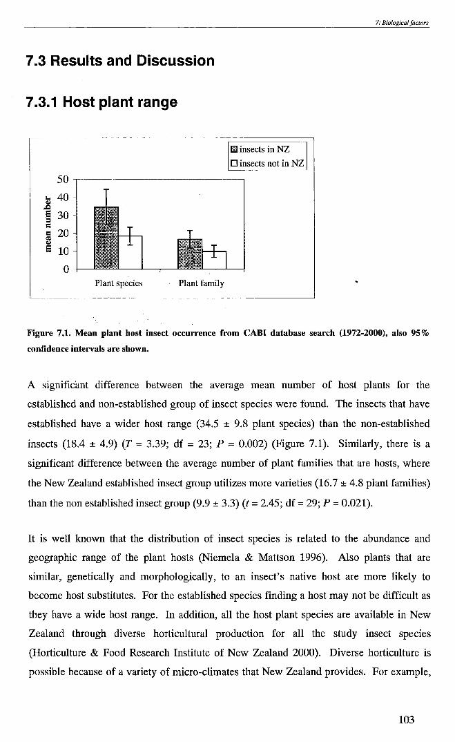
7: Biological factors

7.3 Results and Discussion

7.3.1 Host plant range

iii insects in NZ

D insects not in NZ

50.-----"------------------~

'"' 40 Q,j ,Q

~ 30 = § 20 Q,j

e 10

o Plant species Plant family

Figure 7.1. Mean plant host insect occurrence from CABI database search (1972-2000), also 95%

confidence intervals are shown.

A significant difference between the average mean number of host plants for the

established and non-established group of insect species were found. The insects that have

established have a wider host range (34.5 ± 9.8 plant species) than the non-established

insects (18.4 ± 4.9) (T = 3.39; df = 23; P = 0.002) (Figure 7.1). Similarly, there is a

significant difference between the average number of plant families that are hosts, where

the New Zealand established insect group utilizes more varieties (16.7 ± 4.8 plant families)

than the non established insect group (9.9 ± 3.3) (t = 2.45; df = 29; P = 0.021).

It is well known that the distribution of insect species is related to the abundance and

geographic range of the plant hosts (Niemela & Mattson 1996). Also plants that are

similar, genetically and morphologically, to an insect's native host are more likely to

become host substitutes. For the established species finding a host may not be difficult as

they have a wide host range. In addition, all the host plant species are available in New

Zealand through diverse horticultural production for all the study insect species

(Horticulture & Food Research Institute of New Zealand 2000). Diverse horticulture is

possible because of a variety of micro-climates that New Zealand provides.· For example,

103

7: Biological faclors

tropical fruits can be grown in Northern New Zealand while temperate varieties are grown

elsewhere (Horticulture & Food Research Institute of New Zealand 2000). Similarly, the

non-established insects species may have reduced odds of establishment by having a more

narrow host range. However, this does not fully explain non-establishment as some

sUbtropical species that have not established for example, the scales, Aspidiotus destructor,

Pseudaulacaspis pentagona and Thrips palmi, have a wide host range (Table 2.4). A

possible explanation could be that climate may act on the insect before it has a chance to

reach an available food source or suitable pathways to the plant host may not exist

resulting in insect starvation.

7.3.2 Developmental requirements

Differences between the two study groups of polyphagous insect species-in development

time (degree day requirements) and lower developmental temperature are shown in figures

7.2 and 7.3 respectively. the species that have already established in New Zealand, have

on average a lower developmental threshold (7.4 ± 1.56 °C) and shorter development time

(238.9 ± 135.4 degree days) than the non-established species with a mean of 11.3 ± 2.0 °C

and 393.5 ± 202.1 degree days. These results suggest that insects are more likely to

successfully establish in New Zealand if they are able to tolerate cooler temperatures and

have the ability to develop more quickly. While the difference in mean lower

developmental threshold between the two groups was significant (t = -3.53; df = 14; P = 0.003) there was not a significant difference between mean development times (t = -1.57;

df = 14; P = 0.138) of these groups. This result is reflected in the large confidence

intervals reflecting the high variability of the data and lack of power to detect a difference

if one exists. Clearly a larger sample size is required.

104

7: Biological factors

14

Q) 12 ..... :::I

10 1a ..... Q)

8 0. E Q) 6 +-'

C cu 4 Q)

E 2

0

Insects in NZ Insects not in NZ

Figure 7.2 Average lower developmental thresholds (C) for the two groups of insect species that have

not established (n=8) and those that have (n=10) (see table 2.6 for data). Data were ~vailable for only a

few species in each group. 95% confidence intervals are also shown.

700

600

~ 500 !U "0

1Il 400 .... Cl

~ 300 c: !U

~ 200

100

0-\---

Insects in NZ Insects not in NZ

Figure 7.3 Mean developmental time (in degree days) for the two groups of insect species that have not

established (n=6) and those that have (n=10) (see table 2.6 for data). Data were available for only a few

species in each group. 95 % confidence intervals are also shown.

While there is a significant difference in the average lower developmental threshold

between the two groups of study insects it is recognised that the sample size of the data is

small for specific conclusions concerning the role of the lower developmental threshold

and developmental time in establishment success between the two groups. Clearly more

105

7: Biological faclors

species are needed or more accurate detail about each species is required. Unfortunately

development data is lacking for many species.

A study by Lattin & Oman (1983) suggests that insect species with narrower temperature

tolerance present less of a chance of surviving introductions to new areas than those

species that have a greater tolerance to temperature fluctuations. Indeed the analysis done

here supports that observation. Furthermore, latitude of origin may influence

establishment potential since temperate areas have larger climatic fluctuations than tropical

areas, temperate species especially in the egg/pupa or diapause stage of an insect's life

cycle have higher chances of survival in temperate areas.

7.3.3. Propagule pressure and body size . If we assume that interception rate is an indication of propagule pressure, it appears that

there is no difference in the annual arrival of the insect species that have failed to establish

(2.34 ± 1.94 species per annum) and 'those that have successfully established (2.32 ± 1.37

species per annum) (t = 0.023; df = 40; P = 0.982) (Figure 7.4). It would be interesting to

determine if the propagule pressure for the two groups were historically consistent.

Propagule pressure may play some role in establishment as demonstrated by Berggren

(2001) in his study on the colonisation of Roesel's bush cricket, Metrioptera roeseli

(Hagenbach), into new habitats in Sweden, however, the outcomes from that study were

the result of experimental manipulation. It is possible that stochastic events, for example,

extreme weather may dilute the impact of propagule pressure on establishment. Pimm

(1989) suggests that propagule pressure cannot be relied on as an indicator of

establishment success especially when many accidental introductions have been with small

populations. Pimm (1989) makes this statement, despite that many mathematical models

indicate that small populations have a lower probability of survival especially if popUlation

numbers fluctuate and there is a low rate of intrinsic growth. However, using long-term

census data on the breeding success of bird populations on sixteen British islands, Pimm

(1989) demonstrated that large populations were less sensitive to extinction. Similarly,

Duncan et al. (2001) found a strong relationship between establishment success of birds

and propagule pressure. However in insects, the effect is less clear.

106

7: Biological factors

One must also give consideration to possible Allee effects contributing to the extinction of

very low density populations. There are several mechanisms that ,contribute to the Allee

effect, for example, failure to locate mates, inbreeding depression and predation of

localised small populations (Liebhold & Bascompte 2003). The importance of Allee

dynamics in population extinction has been well studied with respect to the conservation of

endangered species but Liebhold & Bascompte (2003) suggest that it is only recently that

researchers have considered that the combined influences of stochastic processes and Allee

dynamics have some influence in the establishment of invasive species.

4.5

Ql 4 ~ 3.5 ..... c.. Ql 3 u .... Ql ..... 2.5 . ~ ro 2 ::::I C c 1.5 Cll c Cll 1 Ql E 0.5

0 Insects in NZ Insects not in NZ

Figure 7.4 Mean annual interception rate (MAF interception data (1993-1999» for groups of insects

that have yet established (n=114) and those that have established in New Zealand (n=18), 95%

confidence intervals are shown.

Body length measurements derived from literature (see Table 2.5) for insect species that

have not established (n = 12) were on average slightly larger (4.18 ± 2.99 mm) than the

non established species but there is a great deal of variation in body size overall. The

established group of species (n = 13) had on average a smaller body size (2.72 ± 1.10 mm)

but the differences in means were not significant (t = -0.560; df = 15; P = 0.583). While

there appears to be little difference in body size between the two groups of insects, the

sample size is small and there is high variability with insects either particularly small (e.g.

aphids) or at the other extreme, the Coleopteran squash bug, Fabrictilis gonagra (16-19

mm in length) being comparatively large.

107

7: Biological faclors

In general, insect species with higher rates of population increase are thought to have a

higher probability of successful establishment (Crawley 1987, Gaston & Lawton, 1988).

Typically species that have high rates of intrinsic population growth tend to be small

bodied but are susceptible to rapid environmental changes resulting in high variability in

population size. In studies of biological control of weedy species, Crawley (1987) found

that small bodied insects were more successful establishing where they are not normally

found. However no indication of the ranges of body sizes were given and the sample size

of insects that established successfully was relatively small. Gaston & Lawton (1988) also

studied insect body size across taxonomic orders and while they found a negative

relationship between body size and distribution, they concluded that the effect of body size

on population abundance and distribution was inconsistent between taxonomic groups.

They decided that their insect data only weakly supported the theory that small bodied

organisms had an increased probability of survival and establishment.

In another study of nematodes, spiders, molluscs, insects and flatworms introduced into

Britain, Pimm (1989) found a weak positive correlation between body size and successful

establishment. Pimm deduced that smaller bodied organisms were more vulnerable to the

British climate. However, Pimm found that for insects, the smaller bodied species with

high rates of intrinsic population growth did better establishing. Thus for insects, the

intrinsic rate of growth may be a better indicator of establishment success than body size.

However, more specific, rather than general studies based on studying insect genera may

need to be carried out to yield more detailed information on the relationship between body

size and establishment success.

7.4 Taxonomic differences

Figure 7.5 show that the highest interception rates are among insect species belonging to

the families, Diaspidae, Pseudococcidae and Pyralidae (Lepidoptera), but these families

also have the lowest proportion of species establishing. Most species of the Aphididae are

more successful at establishing than any other family. One explanation is that aphid

distribution is greatest in temperate regions, particularly in the Northern Hemisphere

because they are adapted to climates with quite cool winters with many species laying

diapause eggs in autumn. According to Heie (1994), 85% of the total genera of Aphididae

are endemic to the Northern Hemisphere with only 0.4% endemic to· the Southern

108

7: Biological factors

Hemisphere temperate regions (Heie 1994). If aphids from the Northern Hemisphere were

to colonise they would have to quickly produce sexua1es in response to arriving in or near

to the Southern Hemisphere winter. Thus the mode and timing of arrival are very

important for aphid species, especially the egg stage, which is highly suitable for

colonisation as they have long periods of dormancy. Historical records show that once

aphid species arrive in New Zealand, they tend to establish and spread rapidly and become

very difficult to eradicate. For example the blue-green lucerne aphid, Acyrthosiphon

kondoi, Shinji, took I'ess than a year to spread throughout New Zealand (Teulon & Stufkens

2002).

25 D non-established

20 • established

"-CD .0

15 E ::J c: Vl CD

10 ·0 CD a.

r.n 5

0

Figure 7.5. Number of species in each taxonomic family that have either established or failed to

establish in New Zealand (extracted from MAF interception data 1993-1999)

The success of aphid establishment is probably more attributabJe to their parthenogenetic

reproductive strategy, short generation times and ability of winged forms to travel long

distances. The interception data of the 117 species (Table 2.5) shows that the proportion of

insect pests (86%) successfully established in New Zealand reproduce by some

parthenogenic means. In contrast, only 29% of the insect species that have not established

in New Zealand reproduce parthenogenetically (Table 2.5).

109

7: Biological factors

Many studies have searched for the characteristics that increase the chances of insects

establishing in new environments and have hinted that these may be related to taxonomy.

However, such characteristics may not necessarily be reflected in species taxonomy. In a

ten year period (1990-1999) of all imported propagation plant material intercepted at

United States ports, approximately 30% of all arthropods were Homoptera, 9.2% were

Lepidoptera and Thysanoptera accounted for 3.2% (Mack et al. 2002). Insect species

arrivals instead, tend to be a reflection of the number of species within that taxonomic

order associated with the plant material that is likely to be imported. Sailer (1978)

illustrates these observations particularly well by the association of changes in trade and

transport with the different proportions of insect species belonging to major taxonomic

orders arriving into the United States. For example, in 1820 a high abundance of

Coleopterean species arrived because at that time soil was commonly used as ship ballast.

The invention of the steam ship resulted in fast, more efficient trade in plant produce,

increasing the proportion of homopteran insect species establishing (Sailer 1983).

Clear patterns of establishment in taxonomic groups seem to show up well in plants. For

example, most agricultural weeds originate from the large plant families Asteraceae,

Poaceae and Fabaceae (Lattin & Oman 1983). However, there is a lack of evidence

whether this pattern occurs simply by chance or there is a biological reason.

If establishment is related to phylogeny then it might be possible to determine what

particular traits assisted establishment within specific taxonomic groups. Unfortunately

this is a difficult hypothesis to test but some studies have attempted to do just that. For

example, Lattin & Oman (1983) used discriminant analysis to classify 10 life history traits

in 24 cultivated Pinus species- half of which were invasive. The result was the

identification of large seed size and seed production and short juvenile periods as

characteristics of the invasive species. Whilst such predictions about species invasiveness

based on broad taxonomic groupings are useful, the results for insects are certain to be

clouded by environmental interactions and modes of dispersal. Pheloung et al. (1999)

describes a weed risk assessment system that uses information on a plant taxon's current

weed status in other parts of the world, climate and environmental preferences and

biological attributes to assess plant introductions. Some of the attributes are based on the

reproductive and dispersal mechanisms of the plant for example vegetative reproduction

110

7: Biological factors

and minimum generative time, amount of seed production and dispersal by wind or

animals.

7.5 Combining biological and climate variables

Principal component analysis was used with biological and climate variables to determine

if the established and non-established groups could be classified separately based on

combinations of these variables. Table 7.1 shows the principal component loadings

(weights) for each variable and the correlation coefficients (r), after Morrison (1990) for

each component (Chapter 4). Average fecundity per adult and average body length

contribute significantly to the component loadings (r = 0.636 and 0.880 respectively, df = 12, P = 0.05, r critical = 0.553 (after Sachs 1984)). Winter temperature, rainfall, host

range and lower developmental threshold were not significant in their contribution towards

the components.

Table: 7.1. The coefficients of the first and second principle component loadings (weights) for each

variable with the corresponding correlation coefficients (r). The most significant variables are in bold

(Critical value used for r = 0.553 df = 12, P = 0.05, two sided test (after Sachs (1984)). Note that the signs of

the correlation coefficients have been ignored.

Eigenvalue=2.3 Eigenvalue=1.5 Variables Proportion=37.9% Proportion=24.3%

PCI r PC2 r

Minimum (coolest) winter temperature -0.603 0.289 0.217 0.264 Minimum total rainfall -0.433 0.207 -0.158 0.192

Average fecundity per adult 0.072 0.346 -0.522 0.636

Average adult body size -0.006 0.029 -0.726 0.880

Number of plant hosts 0.427 0.204 -0.115 0.140

Lower developmental threshold -0.511 0.245 -0.288 0.351

Figure 7.6 shows the principal component score plots for the 14 species. The horizontal

(x) axis is the first principal component represents winter temperature and lower

developmental threshold (the temperature scale increases from 3 to -4 (coolest to warmest).

The vertical axis (y) is the second principal component representing the biological

variables, fecundity and body size which increase from 2 to -3 (from small body size and

111

7: Biological faclors

low fecundity to larger size and high fecundity). The four quadrants represent four

regimes. The first quadrant (top left in Figure 7.6) consists of insect species that are small

and have low reproductive rates (relative to the overall 14 species) and prefer a mild winter

climate. Their lower developmental thresholds require higher temperatures (again relative

to the overall 14 species), hence in the diagram their developmental threshold is described

as high threshold.

The second quadrant (top right, Figure 7.6) consists of insect species that are smaller and

have low reproductive rates (relative to the overall 14 species) and can tolerate a cool

winter climate. Their lower developmental thresholds are lower (again relative to the

overall 14 species) hence in the diagram their lower developmental threshold is described

as low threshold.

The third and fourth quadrants (bottom in Figure 7.6) consist of the larger insect species

that produce high numbers- of offspring. The lygaeid bug Nysius vinitar is a subtropical

species preferring warm temperatures for growth and development. The weevil, Hypera

pastica, and the introduced moth Epiphyas pastvittana tolerate cool winters and they have

low developmental thresholds.

It is clear from Figure 7.6 that there is a difference between the group of species that have

established in New Zealand (shown by the red dotted line in the figure) and those insect

species that have not established. Predominantly, the species that have established in New

Zealand tend to be small bodied, have relatively low reproduction rates but can survive

cool winter temperatures and have low developmental threshold. However, the PCA must

be interpreted with caution as the data set is small and the variability of the variables for

each species will be important.

112

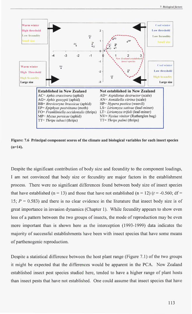
\Varm winter

lI ig h th res hold

1.0\, ft' flllldit~

" 'arm willter

lIig h Th res hold

Large size

Established in New Zealand AC= Aphis craccivora (aphid) AG= Aphis gossypii (aphid) BB= Brevicoryne brassicae (aphid) EP= Epiphyas postvittana (moth) FO= Frankliniella occidentalis (thrips) MP= Myzus persicae (aphid) TT= Thrips tabaci (thrips)

7: Biological faclors

Cool "illh' r

2 Low threshold

1 ,11\\ f"l'lIlIclil,

( '001 \\ ifllt.'r

LIIW threshold

Ili:,!h " ' (' II'HII1\

Not established in New Zealand AD= Aspidiotus destructor (scale) AN= Aonidiella citrin a (scale) HP= Hypera postica (weevil) LS= Liriomyza sativae (leaf-miner) LT= Liriomyza trifoli (leaf-miner) NV= Nysius vinitor (Rutherglen bug) TT= Thrips palmi (thrips)

Large size

Figure: 7.6 Principal component scores of the climate and biological variables for each insect species

(n=14).

Despite the significant contribution of body size and fecundity to the component loadings,

I am not convinced that body size or fecundity are major factors in the establishment

process. There were no significant differences found between body size of insect species

that have established (n = 13) and those that have not established (n = 12) (t = -0.560; df =

15; P = 0.583) and there is no clear evidence in the literature that insect body size is of

great importance in invasion dynamics (Chapter 1). While fecundity appears to show even

less of a pattern between the two groups of insects, the mode of reproduction may be even

more important than is shown here as the interception (1993-1999) data indicates the

majority of successful establishments have been with insect species that have some means

of parthenogenic reproduction.

Despite a statistical difference between the host plant range (Figure 7.1) of the two groups

it might be expected that the differences would be apparent in the PCA. New Zealand

established insect pest species studied here, tended to have a higher range of plant hosts

than insect pests that have not established. One could assume that insect species that have

113

7: Biological faclors

a flexible host range will have a greater chance of survival, providing that the host plants

are present at their new location.

Clearly the lower development threshold and the survivability of insects through winter

cold are key factors in successful establishment in temperate New Zealand. The

established species lower developmental temperature was on average 4 DC lower than

insect species that have not established. Two species, (also apparent in the PCA) Hypera

postica and the leaf-miner Liriomyza trifoli, have similar lower developmental

temperatures to all the established insect species. However, Hypera postica is confined to

the Northern Hemisphere. Unless it can synchronise its life cycle to the seasons within the

Southern Hemisphere, it is unlikely to establish in New Zealand. Liriomyza trifoli, on the

other hand, may be more likely to establish because its global distribution contains many

locations that are climatically similar to New Zealand (Figure 4.2). Also the behaviour of

this species by creating micro-climates within a leaf for protection and its ability to

colonise glasshouses has probably ,contributed to its relative success in establishing

worldwide (R. Baker pers. Comm.). L. trifoli does reproduce sexually and thus its

reproductive strategy may be limiting at some sites, unless both male and female

individuals establish at the same time and at the same site.

114

8: Predictions

8. Comparison of the prediction of insect

establishment into New Zealand by artificial neural

networks and CLIMEX

8.1 Introduction

Initially designed to study the risk of exotic species establishment based on climate

preferences, the computer program, CLIMEX has become an invaluable tool in a wide

range of quarantine services (Sutherst & Maywald 1991). The program can predict an

organism's global distribution based on climate and biological variables and observational

data of its actual geographic distribution. An organism's response towards its

environment, especially during periods of harsh climate conditions, can a"lso be modelled

by generating a series of stress and growth indices (Sutherst & Maywald 1985, 1991,

Sutherst et al. 1999). In CLIMEX the stress indices are based on three climatic

parameters: temperature, moisture and daylength that are then combined into an

'Ecoclimatic index' that describes the overall favourabilty of any location for that

particular organism (Sutherst & Maywald 1985, 1991, Sutherst et al. 1999, also see

Worner 1994).

The extensive literature on CLIMEX discussed in Chapter 3 (MacLeod et al. 2002,

Samways et al. 1999, Baker 1996, Braasch et al. 1996, Boag et al. 1995, Allen et at. 1993,

Sutherst et al. 1991, McFadyen 1991, Panetta & Mitchell 1991, Worner et at. 1989 Worner

1988, Ralph 1987, Sutherst & Maywald 1986) is a reflection of researcher confidence that

it is a successful tool for pest risk establishment. In contrast, artificial neural networks

(ANN) have never been used to predict insect pest invasion. Only recently have artificial

neural networks been applied to biological problems when conventional statistical methods

have failed (Paruelo & Tomasel 1997, Batchelor 1998). Artificial neural networks are very

complex models that are designed to simulate animal brain function resulting in the ability

to learn from the data (Civco 1993, Lek & Guegan 1999). The structure of artificial neural

networks were discussed in more detail in Chapter 6.

In this chapter artificial neural networks were applied to a typical pest risk establishment

scenario and predictions were compared with the commonly used CLIMEX model. Six

115

8: Predictions

randomly chosen insect pests, three that have already established in New Zealand and three

that have not established were modelled by both artificial neural networks and CLIMEX to

predict their establishment in New Zealand using novel climate data for New Zealand sites.

8.2 Methods

The six insect pest species, three that have not yet established in New Zealand and three

that have already established were randomly chosen from the two study groups of insect

pests (n = 36) (Table 2.3). The non-established insect species used in this study were the

yellow scale Aonidiella citrina, the coconut scale, Aspidiotus destructor, palm thrips,

Thrips palmi. The established insect species consisted of the western flower thrips,

Frankliniella occidentalis, the light brown apple moth, Epiphyas postvittana, and the onion

thrip, Thrips tabaci. The six study insects are illustrated in Figure 8.13 (a-f).

Artificial neural networks

To predict establishment in New Zealand, the best performing, based on Cohen's kappa

statitic, artificial neural network model over the re-randomisations of distribution data (see

Chapter 6 for a description of model architecture, particularly noting Figure 6.1) was

chosen for each insect species. Cohen's kappa statistic (Cohen 1960, Landis & Koch

1977), tests whether the model predictions are better than chance (Forbes 1995, Fielding &

Bell 1997, Collingham et al. 2001) and has been described by Manel et al. (2001) as a

robust indicator of prediction performance (see Chapter 6 for full explanation of the kappa

statistic). The network with the highest kappa statistic across the cross-classifications was

judged to have the best model performance.

Similar to Chapter six, the climate data for neural networks were based on sites where the

insect pests were recorded present and a randomised subset of the data of sites where the

insect species have not been found. The randomised subset was to prevent the model from

making false negative predictions because of the large disparity in recordings between sites

where each species were found present compared with sites where they were not found out

of the 7355 climate sites in the database. For example: the yellow scale Aonidiella citrina

(n = 84 sites, 42 sites present, 42 sites absent), the coconut scale, Aspidiotus destructor (n

= 318 sites), palm thrips, Thrips palmi (n = 140 sites). The established insect species

consisted of, the western flower thrips, Frankliniella occidentalis (n = 318 sites), the light

116

8: Predictions

brown apple moth, Epiphyas postvittana (n = 50 sites, 25 sites present, 25 sites absent) and

the onion thrips Thrips tabaci (n = 494 sites).

Novel meteorological data originating from 281 sites throughout New Zealand were used

as the validation or prediction set (New Zealand Meteorological Service 1983). The output

from each network generated an index of establishment between 0 and 100 for of each

insect species being present at the New Zealand sites. A high establishment index (near

100) indicates that presence at a site is highly likely. A low establishment index (near 0)

shows that insect presence is unlikely. Each species distribution was mapped using

Surfer© Version 7.0 and ESRI®ArcMapTM Version 8.2.

CLIMEX

Details of insect species phenology and climatic conditions within their natural

distrubution were used in CLIMEX to estimate their potential distribution in New Zealand.

Physiological data, such as, the lower developmental threshold and developmental time

(Chapter 2, Table 2.6) derived from literature were incorporated into CLIMEX to estimate

the climatic tolerances of each insect species. Parameters in CLIMEX, derived from

weekly rainfall and temperature data for 2500 locations worldwide in CLIMEX's database

(based on 30 year monthly means from the World Meteorological Organisation (1931-

1960)) were used to estimate an organism's response to temperature, moisture and

daylength. The CLIMEX parameters consist of several growth and stress indices that

describe the potential of each insect species to establish at a particular location. The

growth indices determine the climatic conditions favourable for seasonal popUlation

growth, and the stress indices (cold, hot, dry and wet) are the limiting factors for

establishment. For more detail about these indices, see Suthest & Maywald 1991, and in

particular, the CLIMEX user guide (Sutherst et al. 1999).

The parameters for the CLIMEX indices were initially selected for each insect species

using its physiological data, biological information and behavioural information as a guide

(Table 2.6) and then fine tuned by manually adjusting parameter values until the simulated

geographical distribution coincides as closely as possible with the observed distribution.

Fine-tuning or calibration is an iterative process where the parameters are adjusted until

CLIMEX predictions agree with the observed distributions. In other words this approach

represents inverse or inferential modelling because the growth and stress indices are

117

8: Predictions

inferred from the species response to climate through its geographical distribution, relative

abundance and seasonal phenology (reference?). In this study each model was

parameterised using field observations and empirical data from the available literature.

Once parametisation was complete and CLIMEX represented each species known global

distribution as closely as possible, novel climate data for the New Zealand sites were

introduced into to the model.

Once calibration was completed and the model output closely matched the observed

distributions, novel meteorological data based on 281 sites throughout New Zealand were

introduced to CLIMEX and the model for each species re-run to predict their distribution

in New Zealand.

The output from CLIMEX generates a map showing the eco-climatic index (EI) at each

location. The eco-climatic index, a single number between 0 and 100, derived from the

combination of growth and stress indices, describes the climatic suitability at a geographic

site for each species. An eco-climatic index close to zero indicates that the location is not

suitable. Highly favourable locations will have an eco-climatic index close to 100

however, a value as large as this is very rare and is only achievable under constant and

ideal climatic conditions such as in laboratory incubators. According to Sutherst et al.

(1999), an eco-climatic index greater than 30 at a site is usually favourable for

establishment as there will be parts of the year where the seasonal climate is conducive for

population growth, particularly in spring and summer. (Note that in all the figures of the

global predictions of each model that the ANN had far fewer sites to train on (n = 84 to

494 sites) compared with CLIMEX that had 2 500 locations to be calibrated against.)

8.3 Results

The yellow scale, Aonidiella citrin a

Aonidiella citrina occurs throughout most temperate and subtropical countries, particularly

where its main hosts which consist of citrus species, is cultivated (Waterhouse & Sands

2001). The latitudinal range of the species is between 400S and 45°N (Table 2.4 and Figure

8.1 (a». Artificial neural networks (Figure 8.1 (b» predicted an establishment index

between 50 and 70 at sites in Northern India, Pakistan, in south east Asia, Taiwan and

118

8: Predictions

Cambodia, the southern states of North America, namely Texas, California and Florida and

Northern Iran.

a. actual observed distribution

b.ANN

c. CLIM EX

Figure 8.1. Observed distribution (a) of the yellow scale, Aonidiella citrin a derived from literature

search (Table 2.4). (b) Predictions made by artificial neural network (ANN). Output is an

establishment index (0-100) and (c) is the eco-climatic index (0-100) or suitability of each site for

establishment by CLIMEX. (Note that New Zealand does not feature on this map because the climate

data were kept aside for prediction of the novel sites.)

119

8: Predictions

Aonidiella citrina currently occupIes all these sites. Predictions show that the

establishment index declines southwards and northwards from the equator. Predictions for

establishment were made for Queensland, North Australia and sites in the Central African

Republic and Burkina Faso (Central Africa). Despite Aonidiella citrin a occurring in

coastal southern and central New South Wales (Australia), it has never extended its

distribution to Northern Australia (Waterhouse & Sands 2001) but that is not to say it will

not be given the opportunity. This species has not been recorded in Central Africa.

CLIMEX (Figure 8.1 (c» estimated an eco-climatic index between 50-75 for sites in

Hawaii and central Mexico, where Aonidiella citrin a is currently present. Areas of

moderate suitability (25-50) are in Cambodia, southern coastal China, Papua New Guinea

and Sicily (Italy) where the insect species is recorded present. CLIMEX estimated this

species distribution in Africa, where the species has not yet been recorded southwards from

SON (the equivalent of southern Ethiopia) and in Australia (Perth and Brisbane regions).

ra._A_NN ____________________________ -,ra.~C~L~IM~E~X~ ________________________ ~

• st.blllhment Ind.

• <2, • <so · ""

• <100

ECf'lclim!lllc iOOcx c>rCSLM MishlTK.'flt

x <25

• <50

• < 75

< 10 0

Figure 8.2. Predicted establishment of yellow scale, Aonidiella citrin a in New Zealand using novel

meteorological data at 281 sites. (a) The artificial neural network gives an index of establishment at

each site and (b) CLIMEX predicts the suitability of a site for establishment using an eco-climatic

index.

120

8: Predictions

Figure 8.2 shows the potential of Aonidiella citrina establishment in New Zealand as

predicted by artificial neural networks (a) and CLIMEX (b). Both models predict a low

potential of Aonidiella citrin a establishing in New Zealand. ANN gives an establishment

index of between 25 and 50 for most of New Zealand. CLIMEX gives a very low eco­

climatic index for the whole of New Zealand.

The coconut scale, Aspidiotus destructor

The coconut scale, Aspidiotus destructor is common to tropical and subtropical regions

worldwide (Figure 8.3 (a» with a latitudinal range of between 35°S and 45°N (Table 2.4).

The species is a pest of various tropical crops, particularly coconuts and bananas

(Waterhouse & Norris 1989).

Prediction by artificial neural networks reflects the natural distribution very well. An

establishment index of 75 to 100 was predicted for central Mrica (Ivory Coast, Ghana,

Burkina Faso, Guinea, Congo, Cameroon, north of Madagascar and Reunion Island), for

Central America (Ecuador, Panama, Costa Rica, Nicaragua, EI Salvador and Guatemala)

and including Florida, Mexico and Cuba. In South East Asia, Japan, southern coastal

China, Indonesia (Sumatra and Borneo), and Queensland, Australia also had predictions of

high establishment indices. Low indices of establishment were predicted for Europe and

North America. In these areas, Aspidiotus destructor is currently not established there.

Similar to the ANN model, CLIMEX closely matched the observed geographic range of

Aspidiotus destructor.

With respect to the prediction of establishment of Aspidiotus destructor in New Zealand,

CLIMEX predicted no areas that are eco-climatically suitable (Figure. 8.4 (b». Artificial

neural networks on the other hand, predicted a high index of establishment (75-100) for

sites (between 45.5°S and 41.7°S) on the west coast of the South Island of New Zealand.

Some sites included Manapouri, Milford Sound, Haast, the Hermitage at Mt. Cook, Fox

Glacier and Franz Joseph Glacier, Hokitika, Greymouth and Westport. Since Aspidiotus

destructor is a subtropical species (Waterhouse & Norris 1989), the possibility of

establishment on the west coast of the South Island of New Zealand seems unlikely.

121

a. actual observed distribution

b.ANN

c. CLIMEX

• • • • Ecoclimatic index

x 45

• <S4I

.'" • ~oo

8: Predictions

Figure 8.3. Observed distribution (a) of the coconut scale, Aspidiotus destructor derived from literature

search (Table 2.4). (b) Predictions made by artificial neural network (ANN). Output is an

establishment index (0-100) and (c) is the eco-climatic index (0-100) or suitability of each site for

establishment by CLIMEX. (Note that New Zealand does not feature on this map because the climate

data were kept aside for prediction of the novel sites.)

122

8: Predictions

The average temperatures of the sites on the west Coast range between 6°C and 16°C over

the year. For example, the average winter temperature for Fox Glacier is 6.7°C and the

summer temperature is 14.8°C (NZ Meteorological Service 1980) and would clearly limit

population growth.

The resulting ANN model may be sensitive to the high annual rainfall at these sites

resulting in predicted establishment, particularly if moisture were the dominant variable in

the model. For example, Manapouri receives an average rainfall of 3805 rnrnIyear, Haast,

3455 rnrnIyear, Fox Glacier, 4540 rnrnIyear and Westport, 2192 rnrnIyear (NZ

Meteorological Service 1980) which is similar to the amount of rainfall occurring in

subtropical and tropical areas.

a. ANN b. CLiMEX

Ecoclimillic index O(cstaMlshmcnt

x <25

• <50

• < 75

• <1 00

x

Figure 8.4. Predicted establishment of the coconut scale, Aspidiotus destructor in New Zealand using

novel meteorological data at 281 sites. (a) The artificial neural network gives an index of establishment

at each site and (b) CLIMEX predicts the suitability of a site for establishment using an eco-climatic

index.

123

Palm thrips, Thrips palmi a. actual observed distribution

b. ANN

....

Establishment index

)II < 2S

• < S11

• < 75

• < 100

c. CLIMEX

8: Predictions

Figure 8.5. Observed distribution (a) of the palm thrips, Thrips palmi, derived from literature search

(Table 2.4). (b) Predictions made by artificial neural network (ANN). Output is an establishment

index (0-100) and (c) is the eco-climatic index (0-100) or suitability of each site for establishment by

CLIMEX. (Note that New Zealand does not feature on this map because the climate data were kept

aside for prediction of the novel sites.)

124

8: Predictions

Thrips palmi is distributed in subtropical and tropical regions (Figure 8.5 (a)), some of the

areas include Central Mrica and America, the Caribbean, Florida (North America), South

East Asia, New Caledonia and Hawaii (Waterhouse & Norris 1989, Tsai et al. 1995). This

insect is a pest of many plants within the Cucuribitaceae, Solanaceae and Brassicaceae

(Waterhouse & Norris 1989), and according to McDonald et al. (1999) transmits a number

of plant tospovirus (thrips transmitted plant viruses), for example, watermelon silvery

mottle tospovirus.

Artificial neural networks predicted the current distribution of Thrips palmi with

reasonable accuracy (Figure 8.5 (b)). A 75 to 100 index of establishment was predicted at

the following sites where the insect species is currently present: India, southern Japan,

south coast of China, Queensland (Australia), Bogota in Colombia, Venezuela, Panama

and the Indonesian region (Sumatra and Borneo).

CLIMEX did well to determine suitable sites for Thrips palmi establishment (Figure 8.5

(c)). It correctly identified Florida and Hawaii and other sites where the insect pest was

recorded present. Similar to artificial neural networks, the model indicated potential for

establishment on the Mrican continent, where this species it is not currently present,

particularly areas south of 3<N.

In its prediction of establishment of Thrips palmi in New Zealand, CLIMEX indicated that

there are no areas that are eco-c1imatically suitable (Figure 8.6 (b)). Similar, to Aspidiotus

destructor, the artificial neural network model predicted high establishment indices for

sites on the west coast of the South Island of New Zealand. These sites were: Milford

Sound (44.7°S, Jacksons Bay (44.00S), Fox Glacier (43.50$), Franz Joseph Glacier (43.4°S)

and Otira (42.80$). According to McDonald et al. (1999), it is possible that establishment

can occur at higher latitudes, particularly if suitable host plants are grown in protected

cultivation for example, glasshouses. He predicted the possibility of establishment of

Thrips palmi in the United Kingdom, initially into glasshouses from the importation of

plant material but postulated that in the summer months there was enough thermal energy

to drive development and produce several generations of the pest outside the greenhouse.

In winter months re-infestation could occur back into the glasshouses.

125

8: Predictions

b. CLIMEX

Figure 8.6. Predicted establishment of palm thrips, Thrips palmi in New Zealand using novel

meteorological data at 281 sites. (a) The ar tificial neural network gives an index of establishment at

each site and (b) CLiMEX predicts the suitability of a site for establishment using an eco-climatic

index.

In Norway, there is still debate whether this species has established. In the early 1990s it

was intercepted on Ficus (rainforest fig) in several glasshouses (Parella & Mound 1998).

Several specimens were also found outdoors but their identification has never been verified

(Parella & Mound 1998).

Given that the lower developmental threshold of Thrips palmi has been calculated as

approximately 10.1°C (McDonald et al. 1999), sites in Northland, North Island of New

Zealand would be far more conducive for establishment than the west coast of the South

Island. For example, sites such as Kaitaia and Kerikeri have mild winters (on average

approximately 10°C) and summer temperatures on average around 19°C (NZ

Meteorological Service 1980). However, a similar study by Dentener et al. (2002) using

126

B: Predictions

CLIMEX predicted the establishment of Thrips palmi into the upper North Island,

particularly in Kaitaia, where it was the only location that had an eco-climatic value 2: 30.

The disparity between the two studies may be related to the type of physiological data that

was incorporated into the model. Dentener's et al. lower developmental threshold

temperature was 2°C lower than that used in this study and the cold stress indices were

also lower. According to Samways et al. (1999) the accuracy of CLIMEX predictions will

depend upon the precision of the physiological parameters derived for each species. Often

that precision is dependant on what physiological studies for the species are available in

the literature.

Other sites on the east coast of the South and North Islands for example, Alexandra,

Queenstown, Christchurch, Blenheim, Nelson, Hastings, Napier and Masterton would be

too dry for establishment. All these sites have less than 1000 mm/year -average rainfall

(NZ Meteorological Service 1988). For this species the neural network model once again

appears sensitive to rainfalL

The western flower thrips Frankliniella occidentalis

Frankliniella occidentalis is a species of neartic origin (Loomans et al. 1995) and can be

found throughout North America, Alaska, Hawaii, New Zealand, Australia, Korea, Japan,

Peru, Colombia, Costa Rica, South Mrica, throughout Europe, and as far North as Norway,

Sweden and Finland (Figure. 8.7 (a)). The host range of this insect species is extensive

encompassing many plant families (Gramineae, Liliaceae, Chenopodiaceae,

Amaranthaceae, Brassicaceae, Leguminosae, Malvaceae, Convolvulaceae, Solanaceae,

Curcurbitaceae and Compositae (Yudin et al. 1986).

Artificial neural networks (Figure 8.7 (b)) predict an index of establishment between 50

and 75 for New South Wales (southern Australia), Kuala Lumpar (Malaysia), southern

Japan, Israel, Denmark, Great Britain, Poland and Croatia, also Bulgaria, Turkey, South

Mrica, Ecuador, Colombia, Panama, in the southern states of North America (Georgia,

South Carolina, Louisiana, Arizona), central and west United States, Kansas and Oregon.

Lower indices (25-50) were recorded at the following sites (particularly in Central Mrica)

where the species is not normally found: Kano in Nigeria, Chad, Angola and Madagascar

and also Bhutan (north Asia).

127

a. actual observed distribution

b.ANN

•

F.shi bl ishmcnt indn

I( < 2S

• <so • < 75

• < \00

c. CLIMEX

, '" . ... • 45 .. ,.

8: Predictions

Figure 8.7. Observed distribution (a) of the western flower thrips Frankliniella occidentalis derived

from literature search (Table 2.4). (b) Predictions made by artificial neural network (ANN). Output is

an establishment index (0-100) and (c) is the ecoclimatic index (0-100) or suitability of each site for

establishment by CLIMEX. (Note that New Zealand does not feature on this map because the climate

data were kept aside for prediction of the novel sites.)

128

8: Predictions

The most suitable areas (eco-climatic index of 75-100) predicted by CLIMEX (Figure 8.7

(c» were in Europe (including Norway, Sweden and Finland), South Africa, Zimbabwe

and Kenya, also in the north American states of Georgia, South and North Carolina,

Virginia, New York State, Ohio, Kentucky and Illinois, West coast of Canada (Vancouver

region), Central America and the western (Perth region) and south east coast (below

Brisbane, approximately 27.5°S) of Australia .

• ANN

• "-S"-ta ;-:-;bll-'-;-Sh-""me-"nt~IJn. e

, <25

• <50

• <75

<100

h rI IrvtEX

Ecnctimal)C index "reSUlhlishrnent

x <25

• <50

• < 75

< 100

Figure 8.8. Predicted establishment of the western flower thrips Frankliniella occidentalis in New

Zealand using novel meteorological data at 281 sites. (a) The artificial neural network gives an index

of establishment at each site and (b) CLIMEX predicts the suitability of a site for establishment using

an eco-climatic index.

Flower thrips Frankliniella occidentalis occurs extensively throughout New Zealand

(C.A.B International Institute of Entomology 1961). CLIMEX (Figure. 8.8 (b)) has

129

8: Predictions

predicted that most sites within New Zealand are suitable for survival of this species

(Figure 8.9 (b)). The most favourable areas (50-75 eco-climatic index) are in the northern

North Island, Northland (Cape Reinga, Kaitaia, Warkworth) and the Auckland region

(Auckland city), Bay of Plenty (Whakatane) and on the east coast, Hastings. The less

favourable or marginal sites (0-25 eco-climatic index) are in the Palmerston North area

(west coast of the lower North Island) and in the South Island, around Queenstown

(central Otago) and on the west coast (Fox Glacier, Jacksons Bay, Lake Coleridge) and

Riwaka in Nelson. Figure 8.8 (a) shows that the artificial neural network model predicted

establishment indices of 50-75 for all sites in New Zealand indicating all these sites are

suitable for colonisation of Frankliniella occidentalis.

Both models correctly predicted the widespread distribution of Frankliniella occidentalis

and the species is certainly prevalent in areas such as Canterbury, Central Otago in the

South Island and Bay of Plenty and Auckland in the North Island, confirmed by records

from these areas in the PPIN database (Plant Pest Information Network database, Ministry

of Agriculture and Forestry, New Zealand).

The light brown apple moth, Epiphyas postvittana

The light brown apple moth Epiphyas postvittana is a pest of pome fruit, (for example

apples and pears), stonefruit, citrus and many other horticultural crops, in New Zealand. In

fact it has been associated with 250 plant species (Danthanarayana 1995). Originally a

native to south east of Australia, it spread into western Australia, Great Britain, Hawaii,

New Caledonia and is abundant throughout New Zealand (see Figure. 8.9 (a)).

Sites in Great Britain, Tasmania and South East Australia, where the moth Epiphyas

postvittana resides were correctly predicted by ANN (50-75 establishment index). Low

establishment indices were indicated for sites in Algeria, Greece, northern Iran, and Zaire

where the species is not currently present. However, predictions by the ANN for this

species were probably disadvantaged by the lack of available data for training for this

species.

130

8: Predictions

a. actual observed distribution

b. ANN

••

Esta"tl lishmcnt indn

• < 2~

• < 5(1

• < 75

• < 100

c. CLiMEX

Figure 8.9. Observed distribution (a) of the light brown apple moth, Epiphyas postvittana derived from

literature search (Table 2.4). (a) Predictions made by artificial neural network (ANN). Output is an

establishment index (0-100) and (c) is the eco-climatic index (0-100) or suitability of each site for

establishment by CLIMEX. (Note that New Zealand does not feature on this map because the climate

data were kept aside for prediction of the novel sites.)

131

8: Predictions

CLIMEX in Figure 8.9 (c) closely predicted the sites where Epiphyas postvittana is

established in Australia, Hawaii and New Caledonia but predicted a low ecoclimatic index

(0-25) for Great Britain where the species is currently present. Eco-climatic indices of 25-

50 were indicated for the Mediterranean basin, Uruguay (South America), Mexico and

south east coast of Africa, including South Africa, where the insect species is not

considered established.

a. ANN b. CLlMEX

Figure 8.10. Predicted establishment of the light brown apple moth, Epiphyas postvittana in New

Zealand using novel meteorological data at 281 sites. (a) The artificial neural network gives an index

of establishment at each site and (b) CLIMEX predicts the suitability of a site for establishment using

an eco-climatic index.

For New Zealand, ANN predicted an establishment index of 50-75 for the east coast of the

South Island, including central Otago and Southland and most of the North Island (Figure

8.10 (a)). CLIMEX predicted the majority of North Island sites as eco-climatically

suitable (50-75) and also the upper South Island (Nelson and Blenheim and Kaikoura

l32

8: Predictions

regions), other less favourable sites (25-50) were on the south east coast of the South

Island (Canterbury region and Dunedin) and lake sites near Lakes, Hawea, Tekapo, Pukaki

and Rotoiti east of the Southern Alps (South island). The predicted marginal areas are

mainly in the South Island, particularly on the west coast and in Southland (for example,

Invercargill, Te Anau, Gore and Balclutha). However Epiphyas postvittana does occur in

Southland (Thomas 1984) and according to Danthanarayana (1983) and Danthanarayana et

al. (1995), this species is well adapted to cool environments and thrives well in the more

temperate regions of south east Australia and New Zealand. The lower threshold for

development for this insect has been calculated at approximately 7.s°C (Danthanarayana et

al. 1995) that suggests places in the southern South Island are conducive for population

growth. This species is currently distributed widely around New Zealand.

Onion thrips, Thrips tabaci

Thrips tabaci is a cosmopolitan species (Sastrosiswojo 1991, Loomans et al. 1995) (see

Figure 8.12 (a)) and is extremely polyphagous, infesting approximately 300 plant species

particularly within the plant families of Liliaceae, Brassicaceae and Solanaceae (Loomans

et al. 1995). According to Murai (2000) the Thrips tabaci wide host range is a major

factor contributing to its widespread global distribution.

Both artificial neural networks and CLIMEX (Figure 8.11(b & c)) have correctly predicted

the global distribution. Artificial neural networks predicts an establishment indices of 75-

100 throughout the tropical and sUbtropical region, between 35°S and 40oN. Although

Thrips tabaci is present in the Northwest Territories in Canada (60-62 ON), southern Russia

(59-64 ON) and Kazakstan, CLIMEX has predicted sites in these areas as only marginally

suitable (1-25 eco-climatic index) for thrips establishment, indicating that these areas are

perhaps climate limiting for the species as it has not been observed further than 65°N.

Artificial neural networks also gave low establishment indices for'the above areas.

133

8: Predictions

a. actual observed distribution

b.ANN

c. CLiMEX

Figure 8.11. Observed distribution (a) of onion thrips, Thrips tabaci derived from literature search

(Table 2.4). (b) Predictions made by artificial neural network (ANN). Output is an establishment

index (0-100) and (c) is the eco-climatic index (0-100) or suitability of each site for establishment by

CLIMEX. (Note that New Zealand does not feature on this map because the climate data were kept

aside for prediction of the novel sites.)

134

8: Predictions

Figure 8.12 (a & b) show both model predictions of establishment of Thrips tabaci in New

Zealand. For most sites, ANN predicted an establishment index between 25 and 50.

CLIMEX also indicated most sites as eco-c1imatically viable for Thrips tabaci

establishment. Northland and northern North Island were predicted has having the best

sites for establishment for example Cape Reinga and Kaitaia had eco-c1imatic indices of

50. Given the thrips current distribution is widespread from southern South Island to the

northern tip of the North Island (Plant Pest Information Network (PPIN) database, Ministry

of Agriculture and Forestry, New Zealand) one might expect that some sites would have

scored much higher than 50.

a. ANN h r l I'vI EX

• lEstablishment Ind ••

< <25

• <0O

• <1 5

• <100

Figure 8.12. Predicted establishment of onion thrips, Thrips tabaci in New Zealand using novel

meteorological data at 281 sites. (a) The artificial neural network gives an index of establishment at

each site and (b) CLIMEX predicts the suitability of a site for establishment using an eco-climatic

index.

135

a. Aonidiclla cilrina (adult) (source: University ofCalifomia 2(00)

b. Aspidiotus destructor (source: Kessing et al. 1992)

c. Adult Thrips palmi (source Capinera & Castner 2004)

f. Thrips labaci nymphs feeding on onion (source: Cranshaw 2004)

d. Frankliniella occidentalis (adult) (source: Jones 2004)

e. Epiphyas postvittana (adult male) (source: Painter 2004)

f. Thrips tabaci adult (left) and nymph (right) (source: Sparks 2003)

8: Predictions

Figure 8.13. The non-established insect species illustrated are: (a) yellow scale Aonidiella citrina, (b)

the coconut scale, Aspidiotus destructor, (c) palm thrips, Thrips palmi. Established insects are (d) the

western flower thrips, Frankliniella occidentalis, (e) light brown apple moth, Epiphyas postvittana, and

(t) the onion thrip, Thrips tabaci.

136

8: Predictions

8.4 Discussion

CLIMEX correctly predicted the absence of the currently non-established insect species in

new Zealand; the yellow scale, Aonidiella citrina; the coconut scale, Aspidiotus destructor;

and palm thrips, Thrips palmi. Artificial neural networks however, predicted sites

particularly on the west coast of the South Island as suitable for survival for both

Aspidiotus destructor and Thrips palmi which seems not very probable given that these

species have a currently subtropical distribution.

Both models predicted the occurrence of the already established New Zealand species (the

western flower thrips Frankliniella occidentalis and the light brown apple moth, Epiphyas

postvittana). For Thrips tabaci, artificial neural networks predicted a moderate

establishment index (25-50) while CLIMEX predicted that the North Island was the most . conducive area for this species survival.

It appears that CLIMEX is more successful predicting species distributions than the ANN

model. Unexpectedly, the ANN model predicted sites with high rainfall within New

Zealand as the most suitable for establishment for most insect species. The disparity

between model predictions is clearly related to the different theoretical under-pinning of

the two models. Despite that ANN have greater capacity (over more conventional models)

for solving complex patterns, the models in this study were given only climate variables

for prediction. CLIMEX on the other hand, had at its disposal limiting parameters for each

insect species and these were used alongside climate variables to subjectively but

specifically define each species response to the environment. However, the accuracy of

CLIMEX predictions can be influenced by the precison of the physiological data and the

derived parameters used for each species (Sutherst & Maywald 1985, Samways et al.

1999). This imprecision could result in the discrepancy between the Dentener et al. (2002)

study that also used CLMEX and this study's predictions of Thrips palmi establishment in

New Zealand. The Dentener et al. (2002) study predicted the species establishment in

Northland but in this study no sites were predicted suitable for establishment.

The ANN model was at a disadvantage as they had a much smaller climate database for

training (fitting) than CLIMEX. This is normal procedure to prevent the model from over­

fitting the data. To prevent over-predicting absence, a randomised subset of the data

containing sites where the insects were not found were used for the predictions. ANN also

137

B: Predictions

had to learn the distribution of each insect by scratch without the aid of parameter tuning

and calibration that is carried out by the modeller to fit CLIMEX to the observed insect

distributions.

The discrepancy of the predictions between ANN and CLIMEX, particularly on novel data

for New Zealand is partly due to the fact that the ANN could not be optimised. The use of

a generic architecture (Chapter 6) for all insect species constrained each ANN model and

its predictions. More specific architectures optimised for each individual species are

possible with consequent improvements in predictions. However, this approach was

beyond the time frames for this study. In addition, the novel data used to predict the New

Zealand establishment of the chosen species was not of the same structure as that on which

the ANN trained for pattern recognition. The climate databases for each modelling system

were incompatible, while, for this study it would have been better to use the same climate

databases for both models, for example incorporating the 7500 climate sites into the

CLIMEX database. . This eould not .be achieved because the differences in the climate

variables are too great. CLIMEX utilises minimum and maximum air temperature, rainfall

and humidity to calculate soil moisture indices whereas the climate database used for the

ANN uses different variables. To improve the clarity and usefulness of the output of the

two models a single GIS system, using gridded climatologies should be used to map the

predictions at each site from both models. However because of the complex way in which

the output is produced, particularly in CLIMEX, the use of GIS system was beyond the

scope of this current study.

138

9: General discussion

9. General Discussion

9.1 Pest risk analysis

The results of the studies presented in this thesis have been mainly directed towards the

process known as pest risk assessment. Some discussion of pest risk assessment and pest

risk analysis are required here.

In 1951 a multi-lateral International Plant Protection Convention (IPPC) treaty was set up

to control the spread of plant pests and diseases (Baker et al. (2005)). The treaty has been

signed by 124 countries, including New Zealand (United States Office of Technology

Assessment 1983). The International Plant Protection Convention (IPPC) falls under the

umbrella of the Food and Agriculture Organisation of the United Nations ('fAO). There is

also input from regional plant protection organisations, for example, the Asia and Pacific

Plant Protection Commission (APPPC) that includes New Zealand and Australia, the

European! Mediterranean Plant Protection Organisation (OEPPIEPPO) and the North

American Plant Protection Organisation (NAPPO). The framework of the IPPC treaty sets

guidelines for the regulation of agricultural pests that are harmful to plants or plant

products, including the prevention of their spread (Baker et al. 2005, United States Office

of Technology Assessment 1983, IPPC 1996, Wittenberg & Cock 2001). Within that

framework are guidelines for effective pest risk analysis.

Pest risk analysis (PRA) is the process of evaluating whether a pest should be regulated by

phytosanitary measures based on scientific or economic evidence (Food & Agriculture

Organisation 2003). Included within the PRA is a pest risk assessment which involves the

determination of whether an organism will become a quarantine (regulated) pest and the

evaluation of its introduction potential and economic impact (IPPC 1996, Wittenberg &

Cock 2001, Food and Agriculture Organisation 2003). The IPPC defines three stages in

plant pest risk analysis. These are: initiation, pest risk assessment and pest risk

management (Food & Agriculture Organisation 2003). Initiation consists of determining

whether an organism will be a quarantine pest and pathways that are susceptible to its entry

are identified. Second, a pest risk assessment is carried out to determine if the pest should

be categorised as a quarantine (regulated) pest (for example, does the pest fit the criteria in

the definition for a quarantine pest?). Also the likelihood of 1) entry, 2) establishment and

139

9: General discussion

spread, and 3) whether there will be detrimental economic or environmental effects if the

organism managed to establish are also assessed. Next, the conclusions from the pest risk

assessment are used to decide whether risk management is required and the strength of the

measures to be used. Pest risk management is the process of identifying methods to

prevent/ mitigate impacts of the perceived risk and to evaluate the efficacy of these

methods. Such strategies in the prevention of the perceived risk may include,

phytosanitory measures or procedures, for example, inspection and fumigation of imported

plant material that may harbour quarantine (regulated) or harmful plant pest species.

The ideal pest risk analysis should be able to identify the likelihood of an event or process

and its consequences (United States Office of Technology Assessment 1983). For

example, events with low to moderate likelihood but with serious consequences carry high

risk, but events with high probability of occurrence but with minimal consequences are

associated with low risk (Agriculture, Fisheries & Forestry, Australia 2001, Mack et al

2002). It is clear from much of the literature on invasion biology that we cannot predict

with high confidence whether, when or how invasive species become established in new

locations. Williamson 1996, and Mack et al. 2000 point out it is important to remember

that there is always a degree of uncertainty associated with predicting the probability of

organisms establishing in a new environment. Also that predictions that are generally

based on estimating the probability of establishment will fail to predict the risks associated

with establishment (United States Office of Technology Assessment 1983, Mack et al.

2002). In other words, for a full pest risk analysis, policy makers need to consider, how

much risk of damage or harmful impact is acceptable if an organism were to establish.

Whilst scientific information plays an important role in pest risk analysis, the decision

making process involved with estimating potential risk for a particular insect species is not

always derived by quantitative methods. Many analyses made of the potential threats of

insect pest species are based on qualitative or observational information derived from case

studies (United States Office of Technology Assessment 1983, Mack et al. 2002, Murray

2002). There are attempts to try and fully quantify and attach a probability to the risk of

pest risk establishment; for example, Agriculture, Fisheries and Forestry, Australia (2001)

are experimenting with stochastic models that produce a probability distribution of an

event or impact occurring. However, such models are quite complex and are further

limited by the availability of data and technical resources (Murray 2002).

140

9: Gelleral discussion

9.2 Pest risk analysis in New Zealand

The Biosecurity Act (1993) legislates to prevent deleterious organisms into New Zealand.

The law requires that a risk analysis be carried out before any decisions can be made about

importing merchandise (MAF Regulatory Authority 1996). New Zealand's biosecurity

programme which is overseen by the Ministry of Agriculture and Forestry (MAF) Bio­

security Authority (now Biosecurity New Zealand) is based on the management of risks

pre-border such that most measures are designed to reduce the likelihood of pest incursions

through trade and tourism (Crawley et al. 2001, also described in Chapter 2).

The formal technical assessment for pest risk analysis are provided by the MAF regulatory

Authority, with input from industry, technical and scientific experts from universities and

Crown Research Institutes (MAF Regulatory Authority 1996). New Zealand's plant pest . risk· assessment is based on the guidelines of the IPPC, in that each assessment determines

the likelihood of insect pest establishment (MAF Biosecurity Authority 2001). Below are

the steps involved in a typical plant pest risk analysis for an insect plant pest (MAF

Regulatory Authority 1996):

1. Categorising the species with regard to its potential for economic harm.

2. Determining the probability of an introduction occurring through specific pathways for

example, on imported fruit.

3. The final estimate of risk is categorised (for example, high, medium, low risk) based on

the likelihood of establishment.

Factors that would be taken into consideration are; the probability of survival on the host

whilst in transit, the amount of host imported and the likelihood of infested host being

disposed in high risk places such as horticultural areas (Baker et al. 1993, MAF Regulatory

Authority 1996). Other variables that would be considered are the probability of survival

in host plant matter disposed by individuals travelling to New Zealand and the chances of

the insect finding a new host and lastly the suitability of the New Zealand climate for its

survival (MAF Regulatory Authority 1996).

However, to determine biological survival probabilities, especially the chances of insect

pest transmission to and survival at a disposal site is very difficult. For many species, data

of this nature is often lacking, therefore in some plant pest risk analyses survival

141

9: General discussion

probabilities are based on a number of assumptions (Whyte et al. 1994). Because such

data are lacking, survivability data needs to be collated from controlled experiments for

various insect pest species undergoing risk assessment. For example, Whyte et ai. (1994),

successfully calculated survival rates at disposal sites and the probability of spread of the

long-tailed mealy bug (Pseudococcus iongispinus) (Targioni-Tozzetti) and the light brown

apple moth (Epiphyas postvittana) from a series of controlled experiments at Lynfield,

Auckland.

9.3 Combining multivariate and modelling techniques to

assess pest establishment.

No matter how vigilant the agencies are in their attempts to detect new incursions, some

insect species will remain illusive. Between the years of 1993 and 199~ approximately

135 species of polyphagous plant feeding insects were intercepted at the New Zealand

border (Table 2.3). Of these, 22 species have established at one time or another. The

purpose of this study was to determine if these species possess certain characteristics that

have enabled them to establish here. If these characteristics could be identified then that

would contribute to predictions concerning what types of species could establish in New

Zealand in the future, allowing resources to be more targeted. By comparing climate

preferences and biological parameters between the groups of insect species that have

already established in New Zealand and a group that have not, a prototype decision support

methodology has been developed to help assess the probability of establishment of

polyphagous insects in New Zealand (Figure 9.1). The process consists of a flow diagram

comprising a series of questions that lead to determination if an insect species will

establish. The questions are based on the research in this thesis, which will be discussed

and summarised within the proposed process. However, the flow diagram representing the

decision process needs also to be considered along with other biotic characteristics of the

species as well as that of the new environment. These characteristics will be discussed as

each decision of the flow diagram is considered (Figure 9.1).

142

9: General discllssion

t Establishment ~ NO Host plant range

unlikely """""'- Are the host plant( s) present in New Zealand?

l YES Establishment .J YES Analogous climates

likely ......... Is the insect present, especially in South EastAustralia? (Chapter 3)

! NO NO

Clim ate classification

~ Does part of the insect's gbbal distribution

Establishment fall within a cool temperate and moist climate

unlikely regime defined by the Principal component analvsis? (Chaoter 4)

~YES

Data not good enough ~ NO Is the data adequate?

Get more data .......... Does bootstrapping the data result in a kappa statistic> 0.4 for ANN ?(Chapter 6)

!YES Establishment -II( NO Artificial Neural Network and CLiMEX

unlikely Does an AN N netwa-k and a...IMEX predict the presence ofthe insect in New Zealand?

fES Establishment likely

Figure: 9.1 Prototype decision support methodology for assessing the establishment of polyphagous

insect species arriving in New Zealand.

Are the hosts present in New Zealand?

Throughout this study the importance of abiotic factors, particularly climate have been

emphasised as determinants of insect pest distribution and establishment. However, it is

well recognised that biotic factors play an influential role in the establishment process of

insect species but the degree of importance continues to be debated in literature (see

143

9: General discussioll

Chapters 1 & 7). Clearly the availability of host plants are essential for the survival of any

phytophagous insect species and this study found a significant difference in host plant

ranges with the established insect species having a wider host range (34.5 ± 9.8 plant

species) than the non-established insects (18.4 ± 4.9) (t = 3.39; df = 23; P = 0.002) (Figure

7.1). This result indicates that insect species with a wide host plant range are more likely

to succeed in colonization. If insect species can also adapt to species that are related to its

native hosts, then the likelihood of successful establishment increases further.

Biotic factors other than host availability should also be considered when appraising the

establishment success of an insect species. Significant differences between the groups of

polyphagous insect pest species with regard to their development rates and lower

developmental temperatures were found (Figures 7.2 & 7.3). The insect group that has

-established in New Zealand, has on average a lower developmental threshold (7.4 ±

1.56 C) and shorter development time (238.9 ± 135.4 degree days) than the non established

species with a mean threshold of 11.3 ± 2.0 C and a development time of 393.5 ± 202.1

degree days. Such results suggest that insects able to establish in New Zealand are able to

tolerate on average, cooler temperatures and have the ability to develop more quickly.

However the sample size of the data was too small to be completely confident with this

result.

Assuming that the insect interception rate into New Zealand is indicative of propagule

pressure, it appears that there is no significant difference in the annual arrival of insect pest

species failing to establish (2.34 ± 1.94 species per annum) and those that have

successfully established (2.32 ± 1.37 species per annum) (Figure 7.4). The pineapple

mealybug, Dysmicoccus brevi pes, the bean pod borer, Maruca vitrata and the muscid fly,

Atherigona orientalis have very high arrival rates of 59.29, 53.14 and 17.29 per annum

respectively compared with other species. Despite high annual arrival rates these species

have not yet managed to establish in New Zealand. Although, propagule pressure is

important in the establishment of introduced birds (Pimm 1989, Duncan et ai. 2001), there

is little evidence of propagule pressure being highly influential in insect establishment. In

fact, many studies show that accidental introductions of insect species have been derived

from just a small number of individuals (Simberloff 1989, Shaw & Walker 1996, Grevstad

1999). In addition, detection rates are going to be influenced by sampling effort where the

144

9: General discllssion

species that are considered to be important threats will be searched for or the produce that

they arrive on will be sampled more intensively. Such bias could have influenced the data

cited here.

Crawley 1987, Gaston & Lawton, 1988 suggest that insect species with higher rates of

population increase have a higher probability of successful establishment. A large number

of reports (e.g., Moulton & Pimm 1986, Gaston & Lawton 1988, Williamson & Fitter 1996

and Forys & Allan 1999) suggest that species that have high rates of intrinsic population

growth also tend to be small bodied. However, specific studies done by Forys & Allen

(1999) and Gaston & Lawton (1988) could not demonstrate any clear connection between

insect establishment and body size. Similarly, no significant difference in body size

between species that have established and species that have not established (t = -0.560; df

= 15; P = 0.583) (Table 2.5) was found. But again, the sample size was~small and body

length highly variable, with insects ranging from very small or relatively large.

It was difficult to demonstrate clear taxonomic differences between species arriving in

New Zealand which have failed to establish (n = 117) and those that have already

established (n = 15). The most often intercepted belonged to the families, Diaspidae,

Pseudococcidae and Pyralidae (Lepidoptera), but of these families not many have managed

to establish successfully (Figure 7.5). Species belonging to the family Aphididae were

more successful establishing than any other family but there is a high representation of this

family in the database. One possible explanation is that aphid distribution is greatest in

temperate regions because they are adapted to cooler climates. With regard to taxonomic

patterns, clear taxonomic patterns of establishment have been shown in plants but for

insects there is little evidence from the literature to suggest any pattern.

In this study the only biotic factor that could be considered important for the prototype pest

risk assessment process is the expected requirement of host availability (Figure 9.1). There

was no real evidence to suggest that propagule pressure, body size or phylogeny could

predict establishment success, but clearly these factors are not unimportant. Such factors

should be considered in the PRA process, particularly when there is a high degree of

uncertainty predicting establishment of a specific species.

145

9: General discussion

Is the insect present in an analgous climate, especially in south east Australia?

Using the match climate function in CLIMEX, it was found that many locations within

south east Australia had a climate match of 70% or more with sites in New Zealand. More

important, New Zealand shares approximately 90% of its insect pest species listed in the

CABI database (as of 1999) with the south east Australian region (Table 3.1). The

proximity of New Zealand to south east Australia and close economic ties have clearly

helped facilitate exchanges in insect species between the two countries (Teulon & Stufkens

2002, Kuschel 1990). It is evident that if new insect species were to establish in south east

Australia, it is likely that such species will be able to establish here. A new incursion in

that area should provide an alert to New Zealand biosecurity authorities.

South east Australia however, is not the only potential source of insect species, other areas

which were found to be climatically very similar and share a number of in!liect pest species

to New Zealand were also identified in the study. These regions are located in British

Columbia, East coast United States, United Kingdom, Western Europe, Southern France,

coastal Greece, Italy and Sicily, Morocco, Portugal, Northern Spain, coastal locations

around the Black sea, coastal China, Japan, Central and South America, Kenya, South

Mrica and West Australia (Figure 3.1). Insect species originating from Western Europe

and the East coast of the United States could also be particular threats because New

Zealand already shares 78% and 68% respectively of CABI listed insect pests with these

analogous regions.

Because climate conditions are similar between the analogous regions identified here and

sites in New Zealand, it is considered that insect species from these regions have a high

chance of surviving in New Zealand. However, some analogous regions pose less of a

threat than others, simply because there are fewer opportunities for insect spread,

particularly from tourism or trade. For example, there is little and no direct trade or

tourism between East Mrica and New Zealand. While, many other studies have suggested

that climate similarity is a major factor determining establishment success of insect

species, Sailer (1978) and Simberloff (1989) suggest there is difficulty separating out the

influences of dispersal opportunity and the relationship between migration and patterns of

trade. It is thus obvious that to finalise locations as potential sources of harmful insect

pests, it is recommended that the likelihood of arrival in New Zealand is also estimated by

analysing trade patterns and tourism routes.

146

9: General discussion

Does part of the insect's global distribution fall within the climate regime defined by

the principal component analysis?

It has been shown here that principal component analysis (PCA) has indicated patterns of

insect distribution by reducing the climate data into more meaningful variables that explain

most of the spatial pattern. The climate variables were reduced to two components, one

consisting of the temperature derived variables, the other, moisture derived variables

(Table 4.1). The principal component scores for each site were graphed in two­

dimensional ordinal space and from this, four climate regimes were identified (Figure. 4.2).

These were a warm/dry climate (desert, savannah, Mediterranean type locations), a wet/

warm climate (sub-tropical, tropical areas), a dry/cold climate (dry polar regions or inland

continental areas) and lastly a moist/cool climate representing sites with varying degrees of

wetness and coldness that reflects temperate, maritime climates.

In general, New Zealand has a cool.temperate and moist climate (Figure 4.3). It is no

surprise to find that the global distribution of the insect species established in New Zealand

included sites that fall within the cool temperate and moist climate regime (Figure 4.1).

The majority of the insect species that have not yet established in New Zealand have a

narrower distribution, with most sites present in the warm/dry and tropical climates (Figure

4.4).

Some non-established insect species do occupy sites that have been identified as

climatically similar to New Zealand but so far none of these species have managed to

establish successfully despite their constant interception at the border. Species such as

Liriomyza trifoli (American serpentine leaf-miner), Planococcus citri (citrus mealy bug)

and Pseudaulacaspis pentagona (white peach scale) have many sites within their current

distributions that are analogous but at this stage, little explanation can be offered

concerning their lack of establishment. Lack of establishment is definitely not related to

host availability because there are many host plants available in New Zealand for all these

species. Perhaps it is just a matter of time before these species will be found in New

Zealand (further discussed in Section 9.4).

147

9: General discussioll

Does the artificial neural network or CLlMEX predict insect establishment?

Originally used to solve engineering problems, artificial neural networks have been applied

in the biological sciences to solve problems where conventional statistical methods have

had difficulty describing complex, non-linear patterns that often tend to occur in nature

(Pamelo & Tomasel 1997, Batchelor 1998). There is no evidence in the literature of

artificial neural networks used to predict distributions of insect pests, but its potential was

noticed by Worner (pers. comm.). It was found that artificial neural networks predicted

insect presence and absence significantly better than binary logistic regression for 55% of

the species studied here. Binary logistic regression gave predictions better than ANN for

only 13% of species (Table 6.2). Poor predictions for the remainder of the species (32%)

were made by both models.

The kappa statistic was the measure by which the usefulness of model predictions and by

implication, the usefulness of the data for each species was assessed (Figure. 6.3). While

artificial neural network models consistently gave superior results across species than

binary logistic regression, the results were disappointing in that most predictions were only

in moderate or average agreement (0.4 :s k :s 0.7) (Landis & Koch 1977). However, it is

clear that when either method performs badly when the data are bootstrapped then it is

clear the data are not good enough for prediction and that more or better data should be

sought.

Clearly, artificial neural networks have potential to be more accurate but the objective of

this study was to explore the method as an additional tool for pest risk assessment. In this

study a generic architecture was used for all the species to reduce the complexity of

programming and processing time. Using a single architecture for each species constrains

the ANN procedure. Normally, an optimised model would be obtained for each species

but the time and complexity involved with doing this was beyond the scope of this thesis.

Optimised models would most certainly improve the predictions, obtained here.

The coarseness of the geographic scale over which data was collated influences model

accuracy greatly. In this study the distributional data recorded on a regional, provincial or

state level is difficult to determine specific sites within these areas where the insect is

absent. Such data can confuse models into falsely predicting the presence of species at

sites where they tend not to occur (Fielding & Bell 1997). In this study an assumption was

148

9: Gel/eral discussiol/

made that if there was no mention of an insect species presence at a particular geographic

site, it was considered either absent or not yet discovered. More accurate results would be

achieved if insect pest presence or absence are recorded at finer resolutions. Increasing the

awareness of the importance of such data will hopefully result in better data for future

studies on insect distribution. In particular, there is a need to establish true absence in

geographic regions. The interchange of data between international databases on pest

distribution will further improve data availability.

For ANN in particular, poor predictability may be simply that for some species climate

variables may not be such important factors limiting their distribution. In such cases

biological parameters may be more important. It is envisaged that future studies using

ANN will include biological parameters along with climate parameters to enhance

prediction.

9.4 Testing the prototype method

In chapter eight, artificial neural networks were applied to pest risk establishment scenarios

and predictions were compared against the commonly used CLIMEX model. Six insect

species were randomly chosen from the interception database (Table 2.3). Three species

that have established in New Zealand and three that have not established. The insect

species from these case studies are subjected to the prototype decision support

methodology for determining establishment success in New Zealand (Figure 9.1). Table

9.1 summarises the results for each species.

The methodology for determining the likelihood of establishment success correctly

assessed four out of the six insect species. Host plants were available for all six insects so

food availability is not a limiting factor on arrival. The currently established New Zealand

species, western flower thrips, Frankliniella occidentalis, the light brown apple moth,

Epiphyas postvittana, and Thrips tabaci, all reside in south east Australia and other

analogous climate regions, thus the flow diagram correctly assessed their establishment in

New Zealand.

149

9: General discussion

Table: 9.1 Summary of the results using the prototype decision support methodology illustrated in

Figure 9.1. Non-established insects in New Zealand are shown with an asterik (*).

Frankliniella Epiphyas Thrips *Aonidiella *Aspidiotus * Thrips Flow diagram stage

occidentalis postvittana tabaci citrina destructor palmi

Host plant present yes yes yes yes yes yes

Present in south east Australia

and other analogous climates yes yes yes yes no no

Part of global distribution falls

within the cool temperate and yes no

moist climate that typically

makes up New Zealand

Kappa for ANN < 0.4

Predicted present in New

Zealand by ANN or CLIMEX

Establishment outcome likely likely likely likely likely unlikely

The non-established insect Aonidiella citrin a , is currently established in south east

Australia and in eight out of the 15 analogous climates and for this reason the proposed

method (Figure 9.1) suggests its establishment in New Zealand as likely. Currently this

species is not in New Zealand but its global distribution suggests it may be just a matter of

time before a possible establishment occurs.

Aspidiotus destructor on the other hand is not currently established in South East Australia

but part of its global distribution coincides with sites that are climatically similar to the

cool/moist temperate sites in New Zealand. If this species were to establish in south east

Australia then the chances of establishing in New Zealand are probably high.

Thrips palmi is predominantly distributed in subtropical and tropical regions and is not

established in south east Australia, also, this species is not present in sites that are

climatically similar to New Zealand (Figure 4.4). So the method suggests its establishment

is unlikely. It is possible that this species could establish in New Zealand, as there have

been reports of its establishment at higher latitudes, particularly in glasshouses (McDonald

et al. 1999).

150

9: General discussion

9.5 Conclusions and future progress

The studies presented in this thesis have contributed new knowledge and tools for

assessing the establishment of insect species. New analysis tools have been tested on two

groups of insects (established and not established) to determine if they are able to

distinguish between them. Hypotheses concerning the importance of species

characteristics as predictors of invasion success have also been tested. Useful results from

this study have been incorporated into a prototype decision support system but clearly that

system needs refinement. Opportunities to increase the number of species in some of the

studies included here would greatly assist more confident conclusions to be drawn from all

hypothesis tests and analysis methods.

Prediction discrepancies between the ANN (a new tool for eco-climatic assessment) and .. CLIMEX models reflect the need to improve the predictability of ANN and there is indeed

an opportunity to do so by developing specific architectures appropriate to individual

insect species rather than one model for all insect species. It is also important to remember

that ANN and CLIMEX have different theoretical bases and meteorological databases,

CLIMEX includes some biological responses of the species to environmental factors and

uses these to define each insect species' response to the environment more specifically. It

also has a much larger as well as different climate database than was able to be compiled

for the artificial neural network models. In addition, parameter fitting was very different

for each model. CLIMEX relies on fine-tuning or calibration of each parameter by

iterative process until its predictions agree with the observed distributions. Artificial

neural networks on the other hand were at a disadvantage in this study having a smaller

database for training and validation (see Chapters 6 & 8). Unlike CLIMEX that is

calibrated by the user to the observed insect pest distribution, ANN must learn to recognise

patterns between insect presence/absence and climate for each site. If ANN have more

precise climate data and include biological data, then they are sure to give better

predictions when challenged with novel data. However, at this stage both programs are

complimentary, each with the potential to provide insights. In particular, using sensitivity

analysis, ANN could be used along with multivariate statistical analysis to identify factors

that most influence insect distributions. In addition, an important outcome of this study is

the use of bootstrapping that allows the researcher to quickly identify when data are poor

or lacking.

151

9: General discussion

A multidisciplinary approach between ecologists and programmers will enhance the

predictive abilities of ANN and biological interpretation of the outputs. Once the

predictive ability of ANN is advanced further then the prototype decision support method

(Figure 9.1) will also be improved. However, no matter how sophisticated, a pest risk

analysis is not fool-proof and some insect species are bound to defy sophisticated analyses

and well considered determinations. Clearly it is important to keep an open mind with

regard to future tools that become available for pest risk assessment as well as recognise

well used models such as CLIMEX are highly effective and well researched.

152

10: References

10. References Abdulla Koya, KM., Devasahayam, S. & T. Prem Kumar. (199l). Insect pests of ginger

(Zingiber officinale Rosc.) and turmeric (Curuma longa Linn.) in India.

Journal of Plantation Crops. 19(1): 1-13.

Agriculture, Fisheries & Forestry Australia. (2001). Guidelines for Import Risk Analysis

(Draft). Biosecurity Development and Evaluation, Biosecurity Australia;

Canberra

Ajibola Taylor, T. (1967). The bionomics of Maruca testualis Gey. (Lepidoptera:

Pyralidae), a major pest of cowpeas in Nigeria. Journal of the West African

Science Association. 12(2): 111-129.

Alghali, A. (1993). The effects of some agrometeorological factors on fluctuations of the

legume pod borer,. Maruca testulalis Geyer (Lepidoptera: pyralidae). on two

cowpea varieties in Nigeria. Insect Science and its Application.14(1): 55-59.

Allen, J. c., Foltz, L., Dixon, W. N., Liebhold, A. M., Colbert, J. J., Regniere, J. Gray, D.

R., Wilder, J. W., & I. Christie. (1993). Will the gypsy moth become a pest in

Florida? Florida Entomologist.76(1): 102-113.

Amin, A.H. & G.M. Defrawy. (1982). The effects of constant thermohygrographic factors

on the biology of cabbage aphid, Brevicoryne brassicae (Linn.) (Hemiptera:

Homoptera: Aphididae). Zeitschrift fur Angewandte Zoologie. 69(4): 421-428.

Andrewartha, H.G. (1952). Diapause in relation to the ecology of insects. In: Fox Munro,

H., (Ed)., Biological reviews of the Cambridge Philosophical Society. Volume

27. Cambridge. Cambridge University Press. 50-107.

Arnold, c.Y. (1960). Maximum-minimum temperature as a basis for computing heat units.

Journal of the American Society of Horticultural Science. 76: 682-692.

Augustin, N. H., Mugglestone, M. A. & S. T. Buckland. (1996) An autologistic model for

the spatial distribution of wildlife. Journal of Applied Ecology. 33: 339-347.

Austin, M. P. & J. A. Meyers. (1996) Current approaches to modelling the environmental

niche of eucalypts: implication for management of forest biodiversity. Forest

153

10: References

Ecology and Management. 85: 95-106.

Baker, C. R. (1991). The validation and use of a life-cycle simulation model for risk

assessment of insect pests. Bulletin OEPP/ EPPO Bulletin. 21: 615-622.

Baker, R.H. (1996). Developing a European pest risk mapping system. BulietinOEPP/EPPO

Bulletin. 26: 485-494.

Baker, R.H. (2002). Predicting the limits to the potential distribution of alien crop pests. In:

Hallman, GJ., Schwalbe, c.P., (Eds)., Invasive arthropods in agriculture

problems and solutions. Plymouth, UK. Science Publishers, Inc. 207-240.

Baker, R.H., Cannon, R., Bartlett, P. & I. Barker. (2005). Novel strategies for assessing and

managing the risks posed by invasive alien species to global crop production . .

and biodiversity. Annals of AppliedBiology. 146: 177-191.

Baker, R. T., Cowley, J. M. & D. S. Harte. (1993). Pest risk assessment- a process for the

assessment of pest risk associated with importation of plants and plant

products into New Zealand. Auckland. Lynfield Plant Protection Centre, MAF

Quality Management.

Barlow, c.A. (1962). The influence of temperature on the growth of experimental

populations of Myzus persicae (Sulzer) and Macrosiphum euphorbiae

(Thomas) (Aphididae). Canadian Journal of Zoology . 40: 145-156.

Barlow, N & S. Goldson. (2002). Alien invertebrates in New Zealand. In: Pimentel, D.

(Eds)., Biological invasions economic and environmental costs of alien plant,

animal and microbe species. Florida. CRC Press LLC.

Barlow, N. D., Kean, J.M. & S. L. Goldson. (2003). Biological control lessons: modelling

successes and failures in New Zealand. International Symposium on Biological

Control of Arthropods. USDA. Forest Service FHTET- June 2003.

Barry, R.G. & R.S. Chorley. (1968). Atmosphere, Weather and Climate. Great Britain.

Richard Clay (The Chaucer Press) Ltd.

Baskerville, G.I. & P. Emin. (1969). Rapid estimation of heat accumulation from

maximum and minimum temperatures. Ecology. 50(3): 515-517.

154

10: References

Batchelor, W.D. (1998). Fundamentals of neural networks. In: Peart, RM., Curry, RB.

(Eds)., Agricultural Systems Modelling and Simulation. New York. Marcel

Dekker. Inc. 597-628.

Bazzaz, F. A. (1986). Life history of colonising plants: some demographic, genetic and

physiological features. In: Mooney, H. A Drake J. A (Eds)., Ecological studies

58: Ecology of biological invasions of North America and Hawaii. New York:

Springer - Verlag. 97-109.

Beardsley, J.W. (1962). Notes on the biology of the pink sugar cane mealybug,

Saccharicoccus sacchari (Cockerell), in Hawaii (Homoptera: Pseudococcidae).

Proceedings of the Hawaiian Entomological Society. 18(1): 55-59.

Beardsley, J.W.Jr. & RH. Gonzalez. (1975). The biology and ecology of armoured scales.

Annual Review of Entomology. 20: 47-73.

Beaudoin, L., Morin, J.P., Nguyen, C. & B. Decazy. (1995). Study of underground

Adoretus versutus Har. (Col: Scarabaeidae) populations in Vanuatu: detection

of co-habitation with other white grubs. Journal of Applied Entomology.

119(6): 391-397.

Benediktsson, J. A, Swain P. H., Ersoy, O. K. & D. Hong. (1991). Classification of very

high dimensional data using neural networks. Remote sensing for the nineties:

IGARSS 1990, 10th Annual International Geoscience & Remote Sensing

Symposium. 1269-1272.

Ben-Dov, Y. (1978). Taxonomy of the Nigra scale Parasaissetia nigra (Nietner)

(Homoptera: Coccoidea: Coccidae), with observations on mass rearing and

parasites of an Israeli strain. Phtoparasitica. 6(3): 115-127.

Bennett, S. J., Saidi, N. & D. Enneking. (1998). Modelling climatic similarities in

Mediterranean areas: a potential tool for plant genetic resources and

breedingprogrammes. Agriculture, Ecosystems and Environment. 70: 129-143.

Berg, G.N. (1984). The effect of temperature and host species on the population growth

and potential of the cowpea aphid, Aphis craccivora Koch

155

10: References

(Homoptera:Aphididae). Australian Journal of Zoology. 32: 345-352.

Berggren, A.(2001). Colonization success in Roesel's bush-cricket Metrioptera roeseli: the

effects of propagule size. Ecology. 82(1): 274-280.

Blackburn, T. M. & R P. Duncan. (2001). Determinants of establishment success in

introduced birds. Nature. 414: 195-196.

Blackman, R L. (1974). Life-cycle variation of Myzus persicae (Sulz) (Hom., Aphididae)

in different parts of the world, in relation to genotype and environment.

Bulletin of Entomological Research. 63: 595-607.

Blackman, RL. & V.F. Eastop. (2000). Aphids on the World's crops, an identification and . information guide. England. John Wiley & Sons Ltd.

Boag, B. K., A.Evans, G. W., Yeates; Johns, P.M.& R (1995). Neilson. Assessment of the

global potential distribution of the predatory land planarian Artioposthia

triangulata (Dendy) (Tricladida: Terricola) from ecoc1imatic data. New

Zealand Journal of Zoo logy. 22: 311-318.

Boddy, L. & C. W. Morris. (1999). Artificial neural networks for pattern recognition. In:

Fielding, A. (Eds)., Machine learning methods for ecological applications.

Boston, United States: Kluwer Academic Publishers. 37-87.

Boston, A. N. & D.R Stockwell. (1995). Interactive species distribution reporting,

mapping and modelling using the world wide web. Computer Networks and

ISDN systems. 28: 231-238.

Braasch, H., Wittchen, U. & J. G. Unger. (1996). Establishment potential and damge

probability of Meloidogyne chitwoodi in Germany. OEPPjEPPO Bulletin. 26:

495-509.

Brady, K. B. (2002). Ministry of Agriculture and Forestry: Management of Biosecurity

risks. Report of the Controller and Auditor General. Wellington: The Audit

Office.

Brosse, S. & S. Lek. (1999). Predicting fish distribution in a mesotrophic lake by

156

10: References

hydroacoustic survey and artificial neural networks. Limnology and

Oceanography. 44(5): 1293-1303.

Brown, J. H. (1989). Patterns, modes and extents of invasions by vertebrates. In: Drake, J.

A., Mooney, H. A., di Castri, F., Groves R. H. & F. G. Kruger (Eds).,

Biological invasions: a global perspective. Chichester: Wiley.

Brown, D. & R. Rothery. (1993). Models in Biology: mathematics and Statistics and

Computing. Canada: John Wiley & Son.

Brown, M.T. & H.E. Tinsley. (1983). Discriminant analysis. Journal of Leisure Research.

15: 291-310.

Buckland, S. T. & Elston D. A. (1993). Empirical models for the spatial distribution of . wildlife. Journal of Applied Ecology. 30: 478-495.

Busby, J. B. (1991). BIOCLrM- a, biodimate analysis and prediction system. Plant

Protection Quarterly. 6(1): 8-9.

CAB International. (2004). CAB abstracts. Wallingford, United Kingdom. CAB

International.

CAB International. (2004). CABI crop compendium. Wallingford, United Kingdom. CAB

International.

CAB International Institute of Entomology. (1961). Distribution maps of insect pests.

United Kingom: CAB. International.

Cahill, M. (1992). Eco-climatic assessment of Atherigona orientalis (Diptera) and its pest

potential in New Zealand. Canberra. Department of Primary Industries and

Energy Bureau of Rural Resources.

Cammell, M. E. & J.D. Knight. (1992). Effects of climate change on the population

dynamics of crop pests. In: Begon, M., Fitte,r A. H., MacFadyen, A. (Eds).,

Advances in Ecological research. London: Academic Press. 117-162.

Cameron, P. J., Hill, R. L., Bain, J. & W.P. Thomas. (1993). Analysis of importations for

biological control of insect pests and weeds in New Zealand. Biocontrol

157

10: References

Science and Technology. 3: 387-404.

Capinera, J.L. & J. Castner. (2004). Thrips palmi (photograph). University of Florida.

Division of Plant Industry. Retrieved October 2004.

htpp://creatures.ifas.ufl.edu.

Carpenter, G., Gillison, A.N. & J. Winter. (1993). DOMAIN: a flexible modelling

prodcedure for mapping potential distributions of plants and animals.

Biodiversity & Conservation. 2: 667-680.

Case, T. J. (1996). Global patterns in the establishment and distribution of exotic birds.

Biological Conservation. 78: 69-96.

Charles, J. G. & R. C. Henderson. (2002). Catalogue of the exotic armoured scale insects . .

(Hemiptera: Coccoidea: Diaspididae) in New Zealand. Journal of the Royal

Society ofNewz'ealand. 32(4): 587-615.

Chen, Y., Zhao, J.W., Fan, Q.H., Zhao, J.W. & Q.H. Fan. (1999). Effect of temperature on

development, survival and reproduction of Liriomyza sativae. Chinese Journal

of Applied Ecology. 10(6): 710-712. (Abstract only).

Chon, T. P., Park, Y. S., Moon, K. H. & E. Y. Chao (1996). Patternizing communities by

using an artificial neural network. Ecological Modelling. 90: 69-78.

Chon, T., Park, Y., Kim, J., Lee, B., Chung, Y & Y. Kim. (2000). Use of an artificial

neural network to predict population dynamics of the forest-pest pine needle

gall midge (Diptera: Cecidomyiida). Environmental Entomology. 29:(6): 1209-

1215.

Civco, D. L. (1993). Artificial neural networks for land-cover classification and mapping.

International Journal of Geographic Information Systems. 7 (2): 173-186.

Clausen, C.P. (1978). Introduced parasites and predators of arthropod pests and weeds: a

world review. Agriculture Handbook 480. Washington DC. Unites States

Department of Agriculture.

Cohen, J. A. (1960). A coefficient of agreement for nominal scales. Educational and

Physiological Measurement. 20(1): 37-46.

158

10: Referellces

Colautti, R.L, Ricciardi, A., Grigorovich, LA. & H.I. Macisaac. (2004). Is invasion success

explained by the enemy release hypothesis? Ecology letters. 7:721-733.

Collingham, Y. c., Wadsworth, R. A., Huntley, B. & P. E. Hulme. (2001). Predicting the

spatial distribution of non-indigenous riparian weeds: issues of spatial scale

and extent. Journal of Applied Ecology 37(Supp.1.): 13-27.

Connors, L. M., Kiviat, E., Groffinan, P. M. & R. S. Ostfeld. Muskrat (Ondatra zibethicus)

Disturbance to vegetation and potential net nitrogen mineralisation and

nitrification rates in a freshwater tidal marsh. (2000). The American Midland

Naturalist. 143(1): 53-63 (abstract).

Cook, A., Weinstein P & A. Woodward. (2002). The impact of exotic insects in New

Zealand. In: Pimentel, D. (Ed)., Biological invasions -economic and

environmental costs of alien plant, animal and microbe species. Florida: CRC

Press LLC. 217'-239.

Cottier, N. (1953). Aphids of New Zealand. New Zealand D.S.I.R. Bulletin. (No. 106).

Cotton, S. (2001). Definitions ofbiosecurity terms. Biosecurity. 25: 7-7.

Cox, J. M. (1987). Pseudococcidae (Insecta: Hemiptera). Fauna of New Zealand. (No. 11).

Cranshaw, W. (2004). Thrips palmi nymphs feeding on onion (photograph). Colorado

State University. Retrieved October 2004. www.forestryimages.org.

Crause, C. (1990). The white peach scale, Pseudaulacaspis pentagona (Targioni-Tozzetti)

(Homoptera: Diaspidae), a pest of economic importance on grandilla. Acta

Horticulurae.275: 655-662.

Crawley, M. J. (1987).What makes a community invasible? Gray, A. J., Crawley, M. J.,

Edwards, P. J. (Eds). 26th symposium of the British Ecological Society.

Colonisation, Succession and Stability. London: Blackwell Scientific

Publishers. 429-453.

Crawley, M., Holden, C., Nalder, K. & M. Burnett. (2001). Issues paper: Developing a

Biosecurity Strategy for New Zealand. Wellington. Biosecurity Development

Team.

159

10: Referellces

Daly, H.V., Doyen, J.T. & P.R Ehrlich. (1978). Introduction to Insect Biology and

Diversity. United States. McGraw-Hill Book Company.

Danthanarayana, W. (1975). The bionomics, distribution and host range of the light brown

apple moth, Epiphyas postvittana (Walk.) (Tortricidae). Australian Journal of

Zoology. 23: 419-437.

Danthanarayana, W. (1983). Population ecology of the light brown apple moth, Epiphyas

postvittana (Lepidoptera: Tortricidae). Journal of Animal Ecology. 52: 1-33.

Danthanarayana, W., Gu, H. & S. Ashley. (1995). Population growth potential of Epiphyas

postvittana, the light brown apple moth (Lepidoptera: Tortricidae) in relation to

diet, temperature and c1imate.AustralianJournal of Zoology. 43: 381-394.

Davis, M. A. & K. Thompson (2000). Eight ways to be a coloniser; two ways to be an

invader: a proposed nomenclature scheme for invasion ecology. Bulletin of the

Ecological Society of America. 81(3): 226-230.

Dekle, G.W. (1965). Arthropods of Florida and Neighbouring Land Areas Vol.3 Florida

Armoured Scale Insects. Florida. United States. Florida Department of

Agriculture.

Dentener, P. R, Whiting, D.C. & P. G. Connolly. (2002). Thrips palmi (Thysanoptera:

Thripidae): could it survive in New Zealand? New Zealand Plant protection.

55: 18-24.

Department of Conservation. (1998). Space invaders: a summary of the Department of

Conservation's strategic plan for managing invasive weeds. Wellington.

Department of Conservation.

Dewhurst, C. (1999). Forecasting armyworms in the tropics. Pesticide Outlook. 10 (1): 27-

30.

Di Castri, F. (1989). History of biological invasions with special emphasis on the old

world. In: Drake, J. A., Mooney, H. A., di Castri, F., Groves, R H., Kruger F.

J., Rejmanek, M., Williamson, M. (Eds)., Biological invasions: a global

perspective. United States. John Wiley & Sons Ltd.

160

10: References

Diekmann, M. (1992). Use of climatic parameters to predict the global distribution of

Ascochyta Blight on chickpea. Plant disease. 76(1): 409-413.

Dugdale, J. S. (1988). Lepidoptera- annotated catalogue and keys to family and group taxa.

Fauna of New Zealand. (No. 14).

Duncan, R. P. T. M. Blackburn & c. J. Veltman. (1999). Determinants of geographic range

sizes: a test using introduced New Zealand birds. Journal of Animal Ecology.

68: 963-975.

Duncan, P. R., Bomford M., Forsyth D. M. & L. Conibear. (2001). High predictability in

introduction outcomes and the geographical range size of introduced Australian

birds: a role for climate. Journal of Animal Ecology. 70. 621-632.

Duncan, R. P., Blackburn, T.M. & D. Sol. (2003a). The ecology of bird introductions.

Annual Review of Ecology mid Evolution Systematics. 34: 71-98.

Duncan, R.P., Blackburn, T.M. & P. Cassey. (2003b). Factors affecting the release,

establishment and spread of introduced birds in New Zealand. In: Allen, R. B.,

Lee, W.G. (Eds)., Biological Invasions in New Zealand. Berlin: Springer­

Verlag.

Edelson, J.V. & J.J. Magaro. (1988). Development of onion thrips, Thrips tabaci as a

function of temperature. Southwestern Entomological Society. 13(3): 171-176.

Ehrlich, P.R. (1986). Which animal will invade? In: Mooney, H.A. & Drake, J.A. (Eds).,

Ecological series 58: Ecology of biological invasions of North America and

Hawaii. New York. Springer-Verlag. 79-95.

EI-Ibrahy, M. T., EI-Ziady, S. & A. A. Riad. (1972). Laboratory studies on the biology of

the corn leaf aphid, Rhopalosiphum maidis (Homoptera: Aphidae).

Entomologia Experimentalis et Applicata. 15: 166-174.

Elliot, N.C., Kieckhefer, R.W. & D.D. Walgenbach. (1988). Effects of constant and

fluctuating temperatures on developmental rates and demographic statistics for

the corn leaf aphid (Homoptera: Aphididae). Journal of Economic Entomology

81(5): 1383-1389.

161

10: Referellces

Elton, C.S. (1958). The Ecology of Invasions by Animals and Plants. London. Methuen.

Erkilic, L.B. & N. Uygun. (1997). Development time and fecundity of the white peach

scale, Pseudaulacaspis pentagona, in Turkey. Phytoparasitica. 25(1): 9-16.

Fielding, A. H. & J. F. Bell. (1997). A review of methods for the assessment of prediction

errors in conservation presence/ absence models. Environmental Conservation.

24(1): 38-49.

Fliess, J.L., Cohen, J & B.S. Everitt. (1969). Large sample standard errors of kappa and

weighted kappa. Psychological Bulletin. 72(5): 323-327.

Fliess, J. L. (1975). Measuring agreement between two judges on the presence or absence

of a trait. Biometrics. 31: 651~659.

Food and Agriculture Organisation. (1999). International standards for phytosanitary

measures; Glossary of phytosanitary terms. Rome. Food and Agriculture

Organisation of the United Nations.

Food and Agriculture Organisation. (2003). International standards for phytosanitary

measures. Pest risk analysis for quarantine pests including analysis of

environmental risks. ISPM No. 11 Rev.l. Rome. Food and Agriculture

Organisation of the United Nations.

Foody, G.M. (1992). On the compensation of chance agreement in image classification

accuracy assessment. Photogrammetric Engineering and Remote Sensing. 58:

1459-1460.

Forbes, A. D. (1995). Classification-algorithm evaluation: five performance measures

based on confusion matrices. Journal of Clinical Monitoring. 11(3): 189-206.

Forsyth, D. M. & R. P. Duncan. (2001). Propagule size and the relative success of exotic

ungulate and bird introductions to New Zealand. The American Naturalist.

157(6): 583-595.

Forys, E. A. & c. R. Allen. (1999). Biological invasions and deletions: community change

in south Florida. Biological Conservation. 87: 341-347.

162

10: References

Gaston, K. l. & l. Lawton (1988). Patterns in the distribution and abundance of insect

populations. Nature. 331(February): 709-712.

Gevrey, M., Dimopoulos, I. & S. Lek. (2003). Review and comparison of methods to study

the contribution of variables in artificial neural network models. Ecological

Modelling. 160: 249-264.

Goldson, S. L., Phillips, C.B., McNeill, M.R. & N. D. Barlow. (1995). The potential of

parasitoid strains in biological control; observations to date on Microtonus spp.

intraspecific variation in New Zealand. Proceedings, British Crop Protection

Council Symposium. 63: 49-58.

Goldson, S. L., Phillips, c.B., McNeill, M.R., Proffitt, l.R. & R. P. (2001). Cane.

Importation to New Zealand quarantine of a candidate biological control agent

of clover root weevil. New Zealand Plant Protection. 54: 147-151.

Green, R. E., Osborne, P. E. & E. l. Sears. (1994). The distribution of passerine birds in

hedgerows during the breeding season in relation to characteristics of the

hedgerow and adjacent farmland. f ournal of Applied Ecology. 31: 677-692.

Green, R. E. (1997). The influence of numbers released on the outcome of attempts to

introduce exotic birds to New Zealand. fournal of Animal Ecology. 66: 25-35.

Grevstad, F. S.(1999). Experimental invasions using biological control introductions: the

influence of release size on the chance of population establishment. Biological

Invasions. 1: 313-323.

Gros, P. M. & M. Rejmanek. (1999). Status and habitat preferences of Uganda cheetahs: an

attempt to predict carnivore occurrence based on vegetation structure.

Biodiversity and Conservation. 8: 1561-1583.

Guegan,1. F., Lek S. & T. Oberdorff. (1998) Energy availability and habitat heterogeneity

predict global rivervine fish diversity. Nature. 391: 382-384.

Hackwell, K. & G. Bertram. (1999). Pests and Weeds - the costs of restoring an indigenous

dawn chorus. Wellington. New Zealand Conservation Authority.

Hair, 1. F., Anderson, R. E., Tatham, R. L & W. C. Black (1995). Multivariate data

163

10: References

anlaysis with readings (4th edition). New Jersey, United States. Prentice-Hall,

Inc.

Han, M.W., Lee, J.H. & M.H. Lee. (1993). Effect of temperature on development of the

oriental tobacco budworm, Heliocoverpa assulta Guenee. Korean lournal of

Applied Entomology. 32(2): 236-244. (Abstract only).

Hara, A.H., Niino-DuPonte, R.Y. & C.M. Jacobsen. (2001). Root Mealybugs of

Quarantine Significance in Hawaii. Hawaii. College of Tropical Agriculture &

Human Resources, Cooperative Extension Service Insect Pests IP-6.

Heie, O. E. (1994). Why are there so few aphid species in the temperate areas of the

southern hemisphere? European lournal of Entomology. 91: 127-133.

Henderson-Sellers, A. & P.J. Robinson. (1986). Contemporary Climatology. New York.

John Wiley & Sons, Inc.

Hepner, G. F. (1990). Artificial neural network classification using a minimal training set:

comparison to conventional supervised classification. Photogrammatic

Engineering and Remote Sensing. 56: 469-473.

Heywood, V. H. (1989). Patterns, extents and modes of invasions by terrestrial plants. In:

Drake, J. A, Mooney, H. A., Di Castri, F., Groves, R. H., Kruger, F. J.,

Rejmanek, M., Williamson, M. (Eds)., Biological Invasions: a global

perspective. John Wiley & Sons Ltd. 31-60.

Hilbert, D. W. & B. Ostendorf. (2001). The utility of artificial neural networks for

modelling the distribution of vegetation in past, present and future climates.

Ecological Modelling. 146: 311-327.

Hodgson, C. J & R. C. Henderson. (2000). Coccidae (Insecta: Hemiptera: Coccoidea).

Fauna of New Zealand. 41: 1-264.

Hollander, M. & D. A Wolfe. (1999). Nonparametric statistic methods. New York: John

Wiley & Sons Inc.

Horticulture & Food Research Institute of New Zealand. (2000). Horticulture facts and

figures: fruit, flowers, vegetables. Palmerston North, New Zealand:

164

10: Referellces

HortResearch New Zealand.

Howe, W. L. & A. M. Rhodes. (1976). Phytophagous insect associations with Cucurbita in

Illinois. Environmental Entomology. 5(4): 747-751.

Hughes, J. M & K. A. Evans. (1996). Global warming and pest risk assessment:

Implications of "global environmental change" for crops in Europe. Aspects of

Biology. 45: 339-342.

Hulme, P. E.(2003). Biological invasions: winning the science battles but losing the

conservation war? Oryx. 37(2): 178-193.

Hussey, R.F. (1953). Concerning some North American Coreidae (Hemiptera). Bulletin of

the Brooklyn Entomological Society. 68(2): 28-35.

International Union of the Conservation of nature (IUCN). (1999). IUCN guidelines for the

prevention of biodiversity loss due to biological invasion (Draft).

Ivess, R. J. (2000). Description of the New Zealand Ministry of Agriculture and Forestry's

Biosecurity (Phytosanitary) system. Arable/ Horticultural plants and plant

products. Wellington. NZ MAF Biosecurity Authority.

James, F. C. & C.E. McCulloch. (1990). Multivariate analysis in ecology and systematics:

pancea or pandora's box? Annual Review of Ecology and Systematics. 21: 129-

166.

Jones, J.S. (2004). Frankliniella occidentalis (photograph). University of Arizona.

Cooperative Extension. Retrieved October 2004. http://cals.arizona.edu.

Jongman, R. H., ter Braak, C. J. & O. F. van Tongeren.(1995). Data analysis in community

and landscape ecology. Cambridge, United Kingdom. Cambridge University

press.

Kalshoven, L.G. (1964). The occurrence ofXyleborous perforans (Woll.) and X similes in

Java (Coleoptera, Scolytidae). Beaufortia. 11(141): 131-142.

Kay, M. (2002). Macroecology and the prediction of invasive organisms. Goldson, S. L.,

Suckling, D.M. (Eds)., Defending the green oasis: New Zealand biosecurity

165

10: References

and science. Christchurch, New Zealand. New Zealand Plant Protection

Society Inc.

Keane, R.M. & M.J. Crawley. (2002). Exotic plant invasions and the enemy release

hypothesis. Trends in Ecology and Evolution. 17(4): 164-170.

Kessing, J.L.M. & R.F.L. Mau. (1992). Aspidiotus destructor (phtograph). Honolulu,

Hawaii. Department of Entomology. Retrieved October 2004.

www.extento.hawaiLedu.

Kehat, M & M. Wyndham. (1972). The influence of temperature on development,

longevity and fecundity in the Rutherglen bug, Nysius vinitor (Hemiptera:

Lygaeidae).AustralianfournalofZoology.20: 67-78.

King, C. M. (1990). The handbook of New Zealand mammals. Auckland. Oxford

University Press ..

Kocourek, F., Havelka, J., Berankova, J. & V. Jarosik. (1994). Effect of temperature on

development rate and intrinsic rate of increase of Aphis gossypii reared on

greenhouse cucumbers. Entomologia Experimentalis et Applicata. 71(1): 59-

64. (Abstract only).

Kohavi, R. (1995). A study of cross validation and bootstrap for accuracy estimation and

model selection. In: Mellish, C.S. (Ed)., Proceedings of the 14th International

foint Conference on Artificial Intelligence. Morgan Kaufmann Publishers, Inc.

1137-1143.

Kolar, C. S. & D. M. Lodge. (2001). Progress in invasion biology: predicting invaders.

Trends in Ecology and Evolution. 16(4): 199-204.

Krippendorff, K. (1980). Content analysis an introduction to it methodology. London,

United Kingdom. SAGE Publications.

Kriticos, D. J. (1996). The role of ecological modelling in weed management. Shepherd,

R.c. (Ed). In: Proceedings 11 th Australian weeds conference.

Melbourne.Weed Science Society of Victoria Inc.

Kriticos, D & R. Randall. (2001). A comparison of systems to analyse potential weed

166

10: Referellces

distributions. In: Groves, R., Panetta, F., & I. Virtue (Eds)., Weed Risk

Assessment. Victoria, Australia:. CSIRO Publishing. 61-78.

Kuhar T.P. (2000). Population dynamics, mortality factors and pest status of alfalfa weevil

in Virginia. Unpublished PhD thesis. Blacksburg, Virginia. Faculty of the

Virginian Polytechnic Institute and State University.

Kuschel, G. (1990). Beetles in a suburban environment: a New Zealand case study- DSIR

plant protection report (No.3). Auckland, New Zealand. New Zealand

Department of Scientific and Industrial Research.

Landis, 1. R. & G. G. Koch. (1977). The measurement of observer agreement for

categorical data. Biometrics. 33: 159-174.

Lankin Vega, G. O. (2002) Neural network models for the prediction of Autumn migration

of the cereal aphid Rhopalosiphum padi at Lincoln, Canterbury. Unpublished

thesis for Master of Applied Science. Lincoln University, Canterbury.

Larimore, W. E. & R.K. Mehra. (1985) The problem of overfitting data. Byte. (October):

167-180.

Lattin, J. D. & P. Oman. (1983). Where are the exotic insect threats? In: Wilson, C. L.,

Graham, C. L., (Eds). Exotic plant pests and North Ameican agriculture. New

York: Academic Press. 93-137.

Leather, S.R., Walters, K.F.A. & I.S. Bale. (1993). The ecology of insect overwintering.

Cambridge: Cambridge University Press.

Legendre, P. (1993) Spatial autocorrelation: trouble or new paradigm? Ecology. 74(6):

1659-1673.

Leibee, G. L. (1984). Influence of temperature on development and fecundity ofLiriomyza

trifolii (Burgess) Diptera: Agromyzidae) on celery. Environmental

Entomology. 13(2): 497-501.

Lek, S., Belaud, A., Dimopoulos, I., Lauga, I. & I. Moreau. (1995). Improved estimation,

using neural networks, of the food consumption of fish populations. Marine

Freshwater Research. 46: 1229-1236.

167

10: Referellces

Lek, S., Delacoste, M., Baran, P., Dimopoulos, I., Lauga J. & S. Aulagnier. (1996).

Application of neural networks to modelling nonlinear relationships in ecology.

Ecological Modelling. 90: 9-52.

Lek, S. & J.F. Guegan. (1999). Artificial neural networks as a tool in ecological modelling,

an introduction. Ecological Modelling. 120: 65-73.

Lek-Ang, S., Deharveng, L. & S. Lek.(1999). Predictive models of collembolan diversity

and abundance in a riparian habitat. Ecological Modelling. 120: 247-260.

LePelley, R.H. (1968). Pests of Coffee. London. Longmans Green & Co Ltd.

Liebhold, A. M., MacDonald, W. L., Bergdahl, D. & V.c. Mastro. (1995). Invasion by

exotic forest pests: a threat to forest ecosystems. Forest Science Monograph .. 30. Supplement to Forest Science 41(2): 1-49.

Liebhold, A. & J. Bascompte. (2003). The allee effect, stochastic dynamics and the

eradication of alien species. Ecology letters. 6: 133-140.

Liu, S. & X. Meng. (1999). Modelling development time of Myzus persicae (Hemiptera:

Aphididae) at constant and natural temperatures. Bulletin of Entomological

research. 89: 53-63.

Lodge, D.M. (1993). Biological Invasions: lessons for ecology. Trends in Ecology &

Evolution. 8(4): 133-135

Lonsdale, W. M. (1994). Inviting trouble: Introduced pasture species in northern Australia.

Australian Journal of Ecology. 19: 345-354.

Lonsdale, W. M. (1999). Global patterns of plant invasions and the concept of invasibility.

Ecology. 80(5): 1522-1536.

Loomans, A.J.M., van Lenteran, J.c., Tommasini, M.G., Maini, S. & J. Riudavets. (1995).

Biological control of thrips pests. Wageningen Agricultural University Papers.

95(1): 1-201.

McCullagh, P & J. A. NeIder. (1989). Generalised Linear models, Monographs on

Statistics and Applied Probability. 2nd edition ed. London, United Kingdom.

168

10: References

Chapman & Hall.

McDonald, J.R, Bale, J.S. & F.A. Waters. (1999). Temperature, development and

establishment potential of Thrips palmi (Thysanoptera: Thripidae) in the united

Kingdom. European Journal of Entomology. 96(2): 169-173.

McFadyen, R. E. (1991). Climate modelling and the biological control of weeds:- one

view. Plant Protection Quarterly. 6(1): 14-15.

McGarigal, K. Cushman, S & S Stafford. (2000). Multivariate statistics for wildlife and

ecology research. New York. Springer-Verlag.

MacLeod, A., Evans, H.F. & R H. A. Baker. (2002). An analysis of pest risk from an

Asian longhorn beetle (Anoplophora glabripennis). Crop Protection. 21: 635-. 645.

Mack, RN. (1996). Predicting the identity and fate of plant invaders: emergent and

emerging approaches. Biological Conservation. 78: 107-121

Mack, R. N., Simberloff, D., Lonsdale, W. M., Evans, H., Clout, M & F. Bazzaz. (2000).

Biotic invasions: causes, epidemiology, global consequences and control.

Issues in Ecology. 5. http://esa.sdsc.edu/issues5.html.

Mack, R N., Barrett, S. C. H., Defur, P. L., MacDonald, W. L., Madden, L. V., Marshall

D. S., McCullogh, D. G., McEvoy, P. B., Nyrop, M. P., Reichard, S. E. H.,

Rice, K. J & S. A. Tolin. (2002). Predicting invasions of non-indigenous plants

and plant pests. Washington D.C. National Academy Press.

MAF Regulatory Authority. (1996). Risk analysis, opening the way for safety in

agricultural trade. Wellington. New Zealand. Ministry of Agriculture and

Forestry.

MAF Biosecurity Authority. (2001a). Requirements for the diagnosis and reporting of

organisms intercepted at the border, or within transitional facilities.

Wellington. MAF Biosecurity.

MAF Biosecurity Authority. (2001b). Biosecurity authority policy statement on conducting

169

10: Referellces

import risk analyses and applying them in the development of import health

standards. Wellington, NZ: Ministry of Agriculture & fisheries. Retrieved

December 2001. http://www.maf.govt.nz/biosecurity/pests-diseases/risk -

policy.html.

MAF Biosecurity Authority, (2001c) Plants Biosecurity pest risk assessment standard.

Wellington, NZ. Ministry of Agriculture and Forestry.

MAF Biosecurity Authority. (2002). Border inspection report. Surveillance. 29(2): 8-8.

MAF Biosecurity Authority (Plants) (2002). Changes to plant pest quarantine categories.

Biosecurity.35: 13-13.

Manel, S., Dias, J. M., Buckton, S. T. & S. J. Ormerod. (1999a). Alternative methods for

predicting species. distribution: an illustration with Himalayan river birds.

Journal of Applied Ecology. 36: 734-747.

Manel, S., Dias, J., & SJ. Ormerod. (1999b). Comparing discriminant analysis, neural

networks and logistic regression for predicting species distributions: a case

study with a Himalayan river bird. Ecological modeling. 120: 337-347.

Manel, S., Buckton S. T. & S. J. Ormerod. (2000). Testing large-scale hypotheses using

surveys: the effects of land use on the habitats, invertebrates and birds of

Himalayan rivers. Journal of Applied Ecology. 37: 756-770.

Manel, S., Williams, H. C. & S. J. Ormerod. (2001). Evaluating presence-absence models

in ecology: the need to account for prevalence. Journal of Applied Ecology. 38:

921-931.

Manly, B.J. (1986). Multivariate statistical methods a primer. London. Chapman & Hall.

Mastrorillo, S. Lek, S., Dauba, F. & A. Belaud. (1997). The use of artificial neural

networks to predict the presence of small-bodied fish in a river. Freshwater

Biology. 38: 237-246.

Maywald, G. F. & R. W. Sutherst. (1989). Climex: recent developments in a computer

program for comparing climates in ecology. Proceedings from the Simulation

170

10: References

Society of Australia Inc. Eighth Biennial Conference, 25-27 September 1989.

134-40.

Memmott, J., Fowler, S. V. & R. L. Hill.(1998). The effect of release size on the

probability of establishment of biological control agents: gorse thrips

(Sericothrips staphylinus) released against gorse (UZex europaeus). BiocontroZ

Science and Technology. 8(1): 103-115.

Messenger, P. S. (1959). Bioclimatic studies with insects. Annual Review of Entomology.

4: 183-206.

Messenger, P. S. (1976). Experimental approach to insect-climate relationships. In:

Climate and Rice. Los Banos, Philippines. International Rice Research

Institute.

Metcalf, c.L. & W.P. Flint.. (1962). Destructive and Useful Insects their Habits and

Control. New York. McGraw-Hill Book Company.

Miller, G. W & M.B. Isger . (1985). Effects of temperature on the development of

Liriomyza trifolii (Burgess) (Diptera: Agromyzidae). Bulletin of Entomological

Research. 75: 321-328.

Ministry of Agriculture & Forestry. (2003). See, contain, report, a guide to the New

Zealand Import Health Standard for sea containers from all countries.

Wellington. Ministry of Agriculture & Forestry.

Minitab Reference Manual Release 11. (1996). United States. Minitab Inc.

Morrison, D. F. (1980). Multivariate Statistical Methods (3rd edition). United States.

McGraw-Hill, Inc.

Moulton, M. P. & S. L. Pimm. (1986). Species Introductions to Hawaii. Mooney, H. A.

Drake, J.A. In: Ecology of biological invasions of North America and Hawaii.

New York.Springer-vedag.

Mound, LA & AK. Walker. (1982). Terebrantia (Insecta: Thysanoptera). Fauna of New

Zealand. No. 1.

171

10: References

Murai, T. (2000). Effect of temperature on development and reproduction of the onion

thrips, Thrips tabaci Lindeman (Thysanoptera: Thripidae) on pollen and honey

solution. Applied Entomology and Zoology. 35(4): 499-504.

Murray, N. (2002). Import risk analysis, animals and animal products. Wellington.New

Zealand Ministry of Agriculture & Forestry.

New Zealand Meteorological Service. (1983). Summaries of climatological observations to

1980. New Zealand Meteorological Service Miscellaneous Publication 177.

Niemela, P. & W.J. Mattson (1996). Invasion of North American Forests by European

phytophagous insects. Bioscience. 46(10): 741-753.

Oke, T.R. (1987). Boundary Layer Climates. London. Methuen & Co.Ltd.

Onder, E.P. (1982). Investigations on the biology, food plants, damage and factors

affecting seasonal population fluctuations of Aonidiella species (Homoptera:

Diaspididae) injurious to citrus trees in Izmir and its surroundings. Arastirma

Eserleri Serisi. 43: 1-171. (Abstract only).

Osborne, P. E. & B. 1 Tigar. (1992). Interpreting bird atlas data using logistic models: an

example from Lesotho, Southern Mrica. Journal of Applied Ecology. 29: 55-

62.

Painter, D. (2004). Epiphyas postvittana (adult male)(photograph). Retrieved October

2004. htpp:/ /linus.socs.uts.edu.au.

Panetta, F. D. & N. D. Mitchell. (1991). Bioclimatic prediction of the potential

distributions of some weed species prohibited entry to New Zealand. New

Zealand Journal of Agricultural Research. 34: 341-350.

Parrella, M. P. (1987). Biology of Liriomyza. Annual Review of Entomology. 32: 201-24.

Parrella, M.P. & L.A. Mound. (1998). Thrips palmi on ficus in the Netherlands: separating

fact from fiction. Floraculture. 8(11): 30-33.

Parton, W.J. & lA. Logan. (1981). A model for diurnal variation in soil and au

temperature. Agricultural Meteorology. 23: 205-216.

172

10: References

Paruelo, J.M. & F. Tomasel. (1997). Prediction of functional characteristics of ecosystems:

a comparison of artificial neural networks and regression models. Ecological

Modelling. 98: 173-186.

Pearce J., & S. Ferrier. (2000). Evaluating the predictive performance of habitat models

developed using logistic regression. Ecological Modelling. 133: 225-245.

Pearson B.S. & H.O. Hartley. (1976). Biometrika Tables for Statisticians (Vol 2). England.

Charles & Griffin Company·Ltd for the Biometrika Trust.

Pearson, R. G., Dawson, T. P. & C. Liu. (2004). Modelling species distributions in Britain:

a hierarchial integration of climate and land-cover data. Ecography. 27: 285-

298.

Peck, S. B., Heraty, J., Landry, B. & B. J. Sinclair. (1998). Introduced insect fauna of an

oceanic archipelago: the Galapagos Islands, Ecuador. American Entomologist.

44(4): 219-236.

Pedro, J.B. & B. Morallo-Rejesus. (1980). Biology and feeding preference of tobacco

budworm, Helicoverpa assulta (Guenee). Annals of Tropical Research. 1:

135-141.

Penman, D. R. (1998). Managing a leaky border towards a biosecurity research strategy.

Wellington. Ministry for Research, Science and technology.

Peterson, R. K. D. & S. J. Meyer. (1995). Relating degree-day accumulations to calendar

dates: Alfalfa weevil (Coleoptera: Curculionidae) egg hatch in the North

Central United States. Environmental Entomology. 24(6): 1404-1407.

Petitt, F.L., Allen, J.e. & e.S. Barfield. (1991). Degree-day model for vegetable leafminer

(Diptera: Agromyzidae) Phenology. Environmental Entomology. 20(4): 1134-

1140.

Pham, D. T. & X. Liu. (1995). Neural networks for identification, prediction and control.

London. Springer-Verlag Ltd.

Pheloung, P.e., Williams, P.A. & S.R. Halloy. (1999). A weed risk assessment model for

use as a biosecurity tool for evaluating plant introductions. Journal of

173

10: Referellces

environmental management. 57: 239-251.

Pimm, S. L. & D. P. Bartell. (1980). Statistical model for predicting range expansion of the

red imported fire ant, Solenopsis invicta, in Texas. Environmental Entomology.

9: 653-658.

Pimm, S. L. (1989). Theories of predicting success and impact of introduced species. In:

Drake, J. A., Mooney, H. A, Di Castri, F. Groves, R. H., Kruger F. J.,

Rejmanek, M., Williamson, M., (Eds)., Biological invasions: a global

perspective. John Wiley & Sons Ltd. 351-367.

Rafoss, T. & M-G. Srethre. (2003). Spatial and temporal distribution of bioclimatic

potential for the codling moth and the Colorado potato beetle in Norway:

model predictions versus climate and field data from the 1990s. Agricultural

and Forest Entomology. 5: 75-85.

Ralph, W. (1987). A simple model predicts an insects distribution. Rural Research. 136:

14-16.

Ranga Rao, G.V., Wightman, J.A & D.V. Ranga Rao. (1989). Threshold temperatures and

thermal requirements for the development of Spodoptera fitura (Lepidoptera:

Noctuidae). Environmental Entomology. 18(4): 548-551.

Raworth, D.A. (1984). Population dynamics of the cabbage aphid, Brevicoryne brassicae

(Homoptera: aphididae) at Vancouver, British Columbia 11. Development

fecundity and longevity. The Canadian Entomologist. 116: 871-878.

Reichard, S. (2001). The search for patterns that enable prediction of invasion. In: Groves,

R. H., Panetta, F. D., Virtue, J.G.(Eds)., Weed risk assessment. Victoria,

Australia. CSIRO Publishing.

Rejmanek, M. (1989). Invasibility of plant communities. In: Drake, J. A., Money, H. A, di

Castri, F., Groves, R. H., Kruger, F. J., Rejmanek, M., Williamson, M.(Eds).,

Biological invasions: a global perspective. John Wiley & Sons Ltd. 369-384.

Rejmanek, M. (1995). What makes a species invasive? In: Pysek, P., Prach, k., Rejmanek,

M. (Eds)., Plant invasions general aspects and problems. Amsterdam.

174

10: References

Academic Publishing. 3-13.

Rejmanek, M. (2001). What tools do we have to detect invasive plant species? In: Groves,

R H., Panetta, F. D., Virtue, J.G. (Eds)., Weed risk assessment. Victoria,

Australia. CSIRO Publishing.

Rejmanek, M. & D.M. Richardson. (1996). What attributes make some plant species more

invasive. Ecology. 77(6): 1666-1670.

Richardson, D. M., Pysek, P., Rejmanek, M., Barbour, M. G,. Panetta, F. D. & C. J. West.

(2000). Naturalisation and invasion of alien plants: concepts and definitions.

Diversity and Distribution. 6: 93-107.

Roberts, H. (1977). Observations on the biology of some tropical rainforest Scolytidae . (Coleoptera) from Fiji. II. Subfamily Ipinae- tribe Xyleborini. Journal of

Natural History. 11(3): 251-272.

Rose, D. J. W., Dewhurst, C. F. & W. W. Page. (1995). The bionomics of the Mrican

armyworm Spodoptera exempta in relation to its status as a migrant pest.

Intergrated Pest Management Reviews. 1(1): 49-64.

Rumelhart, D. E., Hinton, G. E. & R J. Williams. (1986). Learning representations by

back-propagating errors. Nature. 323: 533-537.

Sach, L. (1984). Applied statistics: a handbook of techniques (2nd edition). Berlin.

Springer-Verlag. 424-425.

Saha, S. & D. Raychaudhuri. (1997). Factors affecting Aphis gossypii Glover. population

on chilli, capsicum annum L. Research Bulletin of the Paqnjab University.

Science. 47(1-4): 171-197.

Sailer, R T. (1978). Our immigrant fauna. Bulletin of the Entomological Society of

America. 24(1): 3-11.

Sailer, RT. (1983). History of Insect Introductions. In: Graham, c., Wilson, C. (Eds).,

Exotic plant pests and North American Agriculture. New York. Academic

Press. 15-38.

175

10: Referellces

Sakai, A. K, Allendorf, F.W., Holt, J.S., Lodge, D.M., Molofsky, J., With, KA.,

Baughman, S., Cabin, J.E., Cohen, N.C., Ellstrand, D.E., McCauley, P.,

O'Neil, 1. M., Parker, J,. Thompson, N. & S. G. Weller. (2001). The population

biology of invasive species. Annual Review of Ecological Systematics. 32:

305-332.

Samways, M.J., Osborn, R., Hastings, H. & V. Hattingh. (1999). Global climate change

and accuracy of prediction of species' geographical ranges: establishment

success of introduced ladybirds (Coccinellidae), Chilocorus spp.) worldwide.

Journal of Biogeography. 26: 795-812.

Samways, M.J. (2003). Critical response from Professor Michael J. Samways. Journey of

Biogeography. 30: 817.

Sastrossiswojo, S. (1991). Thrips on vegetables in India. In: Talekar, N.S. (Ed)., Thrips in

Southeast Asia. Proceedings of a Regional Consultation Workshop, Bangkok,

Thailand. Taipei. Asian Vegetable Research and Development Centre: 12-17.

Sax, F.D. & lH. Brown. (2000). The paradox of invasion. Global Ecology and

Biogeography. 9: 363-371.

Schroder, R F. W. & A.L. Steinhauer. (1976). Effects of photoperiod and temperature

regimens on the biology of European and United States Alfalfa weevil

populations. Annals of the Entomological Society of America. 69(4): 701-706.

Scott, RR & RM. Emberson. (1999). Handbook of New Zealand Insect Names, Common

and Scientific Names for Allied Organisms. Auckland, NZ. Entomological

Society of New Zealand.

Shaw, P. W. & J. T. S. Walker. (1996). Biological control of woolly apple aphid by

Aphelinus mali in an intergrated fruit production programme in Nelson.

Proceedings of the 49th New Zealand Plant protection conference: The New

Zealand Plant Protection Society Inc.

Shea, K & P. Chesson. (2002). Community ecology theory as a framework for biological

invasions. Trends in Ecology & Evolution. 17(4): 170-176.

176

10: References

Simberloff, D. (1986). Introduced insects: a biogeographic and systematic perspective. In:

Mooney, H. A., Drake, J. A, (Eds)., Ecological series 58: Ecology of

biological invasions of North America and Hawaii. New York. Springer­

Verlag. 3-26.

Simberloff, D. (1989). Which insect introductions succeed and which fail. In: Drake, J. A.,

Mooney, H. A, Di Castri, F., Groves, R. H., Kruger, F. J., Rejmanek, M.,

Williamson, M., (Eds)., Biological invasions: a global perspective. John Wiley

& Sons Ltd. 61-75.

Skinner, K. M. & R. D. Child. (2000). Multivariate analysis of the factors influencing

changes in Colorado grasshopper abundances. Journal of Orthoptera Rsearch:

103-109.

Slosser, l, Pinchak, W. & D.Rummei. (1998). Biotic and abiotic regulation of Aphis

gossypii Gloverin west Texas dryland cotton. Southwestern. 23(1): 31-65.

Smallwood, K. S. (1994). Site invasibility by exotic birds and mammals. Biological

Conservation. 69: 251-259.

Songa, J. M., Zhou, G.F., Overholt, W. A. & G.F. Zhou. (2001) Relationships of stemborer

damage and plant physical conditions to maize yield in a semi-arid zone of

Eastern Kenya. Insect Science and its Application. 21(3): 243-249 (abstract).

Sparks, AN. Jr. (2003). Thrips tabaci adult and nymph (photograph). University of

Georgia. Retrieved October 2004. www.forestryimages.org.

Stockwell, D. & D. Peters. (1999). The GARP modelling system: problems and solutions

to automated spatial prediction. International Journal of Geographical

Information Science. 13(2): 143-158.

Sutherst, R. W. & G. F. Maywald. (1985). A computerized system for matching climates in

ecology. Agricultural Ecosystems and Environment. 13: 281-299.

Sutherst, R. W. & G. F. Maywald. (1991). Climate modelling and pest establishment,

Climate-matching for quarantine, using CLIMEX. Plant Protection Quarterly.

6(1): 3-7.

177

10: References

Sutherst, R. W., Maywald, G.F. & W. Bottomley. (1991). From climex to pesky, a generic

expert system for pest risk assessment. Bulletin OEPP/ EPPO Bulletin. 21:

595-608.

Sutherst, R. W., Maywald, G.F. & D. B. Skarratt. (1995). Predicting insect distributions in

a changed climate. In: Harrington, R., Stork, N.E. (Eds)., Insects in a changing

environment. London Academic Press Ltd. 59-91.

Sutherst, R. W., Maywald, G.F., Yonow, T. & P. M. Stevens. (1999). Climex- Predicting

the effects of climate on plants and animals- User guide. Victoria, Australia.

CSIRO Publishing.

Sutherst, R.W. (2003). Prediction of species geographical ranges. Journal of

Biogeography. 30: 805-816.

Sutherst, R.W. & G. Maywald. (2005). A climate model of the red imported fire ant,

Solenopsis invicta Buren (Hymenoptera: Formicidae): Implications for

invasion of new regions, particularly Oceania. Environmental Entomology.

34(2): 317-335.

Swets, J. A. (1988). Measuring the accuracy of diagnostic systems. Science. 240: 1285-

1293.

Sykes, M. T., Prentice, I.C. & W. Cramer. (1996). A bioclimatic model for the potential

distributions of north European tree species under present and future climates.

Journal of Biogeography. 23: 203-233.

Taylor, T,A. (1967). The bionomics of Maruca Testualis Gey. (Lepidoptera: Pyralidae), a

major pest of cowpeas in Nigeria. Journal of Biogeography. 12(2): 111-129.

Teulon, D. A. J. & M. A. W. Stufkens. (2002). Biosecurity and aphids in New Zealand.

New Zealand Plant Protection. 55: 12-17.

The International Plant Protection Convention (IPPC). (2003). International Plant

Protection Convention. Food and Agriculture Organisation of the United

Nations (FAD). Retrieved January 2004. http://www.ippc.int.

Thomas, W.P. (1984). Light brown apple moth, Epiphyas postvittana (Walker) lifecycle

178

10: Referellces

(1st Revision). New Zealand Department of Scientific and Industrial Research.

DSIR Information Series No. 105/3.

Thornthwaite, W.e. (1933). The climates of the earth. The Georaphical Review. 23: 433-

440.

Thornthwaite, W.C. (1948). An approach toward a rational classification of climate. The

Geographic Review. 38: 55-94.

Tsai, lH., Bisong, Y., Webb, S.E., Funderburk, J.E. & H.S.U. Hei Ti. (1995). Effects of

host plant and temperature on growth and reproduction of Thrips palmi

(Thysanoptera: Thripidae). Environmental Entomology. 24(6): 1598-1603.

United States Department of Commerce (2002). National Oceanic and Atmospheric

Administration. Retrieved June 2002.

http://www.ngs.noaa.gov/pub/pcsoft/for _ inv.3d

United States Congress, Office of Technology Assessment. (1983). Harmful non­

indigenous species in the United States. Washington D.C. U.S. Government

Printing Office.

University of California, State wide intergrated pest management. (2000). Adult,

Aonidiella citrina (photograph). Retrieved October 2004.

www.imp.ucdavis.edu.

Usinger, R.B. (1942). The genus Nysius and its allies in the Hawaiian Islands (Hemiptera,

Lygaedidae, Orsillini). Bernice P. Bishop Museum Bulletin 173.

Van Duyn, J. & M. Murphey. (1971). Life history and control of white peach scale,

Pseudaulacaspis pentagona (Homoptera: Coccoidea). The Florida

Entomologist. 54(1): 191-195.

Velasquez, F.J. (1971). Some Philippine armoured scale insects of the tribe Aspidiotini

(Diaspididae: Homoptera). The Philippine Entomologist. 2(2): 89-154.

Veltman, e. J., Nee, S. & MJ. Crawley. (1996). Correlates of introduction success in

exotic New Zealand birds. The American Naturalist. 147(4): 543-557.

179

10: References

Vera, M.T., Rodriguez, R, Segura, D.P., Cladera, J.L. & RW. Sutherst. (2002). Potential

geographical distribution of the Mediterranean fruit fly, Ceratitis capitata

(Diptera: Tephritidae), with emphasis on Argentina and Australia.

Environmental Entomology. 31: 1009-1022.

Verrneij, G. J. (1996). An agenda for invasion ecology. Biological Conservation. 78: 3-9.

Vitousek, P.M. (1988). Diversity and biological invasions of oceanic islands. In: Wilson,

E.O. (Ed)., Biodiversity. Washington D.C. National Academy Press.

Vitousek, P. M., Dantonio, c.A., Loope, L.L., Rejmanek, M. & R Westbrooks. (1997).

Introduced species: a significant componenet of human-caused global change.

New Zealandlournal of Ecology. 21(1): 1-16.

Wagner, T., Dapper, T. & H. H. Schmidt. (2000). The influence of environmental variables

on the abundance of aquatic inseCts: a comparison of ordination and artificial . .

neural networks. Hydrobiologia. 422: 143-152.

Walker, P. A. & K. D. Cocks.(1991). HABITAT: a procedure for modelling a disjoint

environmental envelope for a plant or animal species. Global Ecology and

Biogeography Letters. 1: 108-118.

Ward, M. P. (1994). The use of discriminant analysis in predicting the distribution of

bluetongue virus in Queensland, Australia. Veterinary Research

Communications. 18: 63-72.

Waterhouse, D.F. & K.R. Norris. (1989). Biological control Pacific prospects -

supplement 1. Canberra. Australia. Australian Centre for International

Agriculture Research.

Waterhouse, D. F & D. P. A. Sands. (2001). Classical Biological control of Arthropods in

Australia. Canberra. CSIRO Publishing.

Whyte, C. F., Adams, R L., Richmond, J. E., Cowley, J. M. & R T. Baker. (1994).

Experimental analysis of pest risk factors- an analysis of some biological

survival factors used in pest risk assessment. Auckland. Lynfield Plant

Protection.

180

10: References

Wilcoxon, F., Katti, S.K. & R.A. Wilcox. (1973). Critical values and probability levels for

the Wilcoxon rank sum test and the Wilcoxon signed rank test. In: Harter,

H.L., Owen, D.B. (Eds)., Selected tables in mathematical statistics, (vol 1).

Providence, Rhode Island. American mathematical society and Institute of

mathematical statistics. 171-260.

Williams, D. J. (1982). The distribution of the mealybug genus planococcus (Hemiptera:

Pseudococcidae) in Melanesia, Polynesia and Kiribati. Bulletin of

Entomological Research. 72: 441-455.

Williams, B. K & K. Titus. (1988). Assessment of sampling stability in ecological

applications of discriminant analysis. Ecology. 69(4): 1275-1285.

Williams, D.J. & G.W. Watson. (1988). The Scale Insects of the Tropical South Pacific

Region. Part 2: The Mealybugs (Pseudococidae). London. C.AB.

International.

Williams, D. W & A M. Liebhold.(1997). Latitudinal shifts in spruce budworrn

(Lepidoptera: Tortricidae) outbreaks and spruce-fir forest distributions with

climate change. Agriculture and Forest Entomology. 32(1-2): 205-215.

Williams, D. W & A. M. Liebhold.(2002). Climate change and the outbreak ranges of two

North American bark beetles. Agricultural and Forest Entomology. 4: 87-99.

Williamson, M. (1993). Invaders, weeds and the risk from genetically manipulated

organisms. Experentia. 49: 219-224.

Williamson M. (1996). Biological Invasions. London. Chapman & Hall.

Williamson, M. H. Fitter A (1996a). The characters of successful invaders. Biological

Conservation. 78: 163-170.

Williamson, M. & A Fitter. (1996b). The varying success of invaders. Ecology. 77(6):

1661-1666.

Wilson, L. & Barnett, W.W. (1983). Degree-days: an aid in crop and pest management.

California Agriculture. 37(1-2): 5-7.

181

10: Referellces

Wittenberg, R & M. J. W. Cock (Eds). (2001). Invasive Alien species- a toolkit of best

prevention and management practice (Global Invasive Species Programme

(GISP). Wallingford, United Kingdom. CAB International..

Worner, S. P. (1988). Ecoclimatic assessment of potential establishment of exotic pests.

Journal of Economic Entomology. 81: 973-983.

Worner, S. P. (1991). Use of models in applied Entomology: The need for perspective.

Environmental Entomology. 20(3): 768-773.

Worner, S. P. (1994). Predicting the establishment of exotic pests in relation to climate. In:

Sharp, J.L., Hallman, G.J. (Eds)., Quarantine treatments for pests of food

plants. Westview. Colorado. Boulder Press. 11-32.

Wotner, S. P. (2002) Predicting the invasive potential of exotic insects. In: Hallman, G. J.,

Schwalbe, c.P. (Eds)., Invasive arthropods in agriculture problems and

solutions. Enfield (NH), USA. Science Publishers, Inc. 119-137.

Worner, S. P., Goldson, S.L. & E. R. Frampton. (1989) Comparative ecoclimatic

assessment of Anaphes diana (Hymenoptera: Mymaridae) and its intended host

Sitona discoideus (Coleoptera: Curculionidae) in New Zealand. Journal of

Economic Entomology. 82: 1085-1090.

Worner, S. Lankin G. Samarasinghe S. & D. Teulon. (2001). Improving prediction of

aphid flights by temporal analysis of input data for an artificial neural network.

New Zealand Plant Protection. 54: 188-192.

Wu, 1.J., Zhang, W.O., Liang, G.W., Zhang, W.O. & G.W. Liang. (1995). Journal of South

China Agricultural University. 16(4): 14-19. (Abstract only).

Xia, IY., van der Werf, W. & R. Rabbinge. (1999). Influence of temperature on bionomics

of cotton aphid, Aphis gossypii, on cotton. Entomologia Experimentalis et

Applicata.90: 25-35.

Yamada, Y., Sakurai, H., Tsuchida, K. & A. Inoue. (1996). Effects of temperature and

food plants on development of alfalfa weevil, Hypera postica. Research

Bulletijn of the Faculty of Agriculture, Gifu University. 61: 39~44. (Abstract

182

10: References

only).

Yarro, J. G. (1984). Life and fertility tables for Spodoptera exempta (WLK) (Lepidoptera,

Noctuidae). Insect Science and its Application. 5(4): 303-305.

Yudin, L.S., Cho, J.J. & W.e. Mitchell. (1986). Host range of western flower thrips,

Frankliniella occidentalis (Thysanoptera: Thripidae), with special reference to

Leucaena glauca. Environmental Entomology. 15(6): 1292-1295.

Zhang, R.J., Yu, D.J. & c.O. Zhou. (2000). Effects of temperature on certain population

parameters of Liriomyza sativae Blanchard (Diptera: Agromyzidae ).

Entomologia-Sinica. 7(2): 185-192. (Abstract only).

Zhou, e.A., Zou, J.J. & J.e. Pengo (1993). Bionomics of coconut scale - a main pest insect -

onActinidia and its control. Entomological Knowledge. 30(1): 18-20.

Xie, L.Q., Jiang; M.x., Zhang, X.x., Xie, L.Q., Jiang, M.x. & x.x. Zhang. (1998). Effect

of temperature and humidity on laboratory population of H eliocoverpa assulta.

Acta Entomologica Sinica. 41(1): 61-69. (Abstract only).

183

11: Appendices

11. Appendices

Appendix I List of the polyphagous insect species that have been intercepted in New Zealand (1993-1999).

E= the insect is established in New Zealand

M= CAB! distribution map of the insect is available

T= the insect has been re-classified or has a synonym

Insects sampled but rejected from the study are under-lined

Insects sampled and accepted for further study are in bold

Annual No. of Species Common name Order Family intercepton CABI

rate records

Abragallas{lis cy'ano12hy}li armoured scale Hemiptera Diaspididae 0.43 0

Abragallaspis musae armoured scale Hemiptera Diaspididae 0.43 0

Abragallaspis subchortina arinoured scale ' Hemiptera Diaspididae 0.14 0

M Adoretus versutus compressed beetle Coleoptera Scarabaeidae 0.43 11

M Alearodicus dispersus spiraling whitefly Hemiptera AJeyrodidae 0.29 0

Anaphothrips dubius thrips Thysanoptera Thripidae 0.29 0

M Aonidiella citrin a yellow scale Hemiptera Diaspididae 0.43 52

Aphanocorynes humeralis weevil Coleoptera Curculionidae 0.14 0

EM Aphis craccivora cowpea aphid Hemiptera Aphididae 2.00 1262

EM Aphis gossypii cotton aphid Hemiptera Aphididae 11.86 2595

Aphodius liuidis beetle Coleoptera Scarabaeidae 0.14 0

T A{lhomia gularis stored nut moth Lepidoptera Pyralidae 0.14 3

Araecerus fasciculatus beetle Coleoptera Anthribidae 2.57 107

M Aspidiella hartii yam scale Hemiptera Diaspididae 9.29 17

M Aspidiotus destructor coconut scale Hemiptera Diaspididae 7.29 79

Aspidiotus excisus armoured scale Hemiptera Diaspididae 0.57 0

Aspidiotus musae armoured scale Hemiptera Diaspididae 0.43 0

Aspidiotus pacificus armoured scale Hemiptera Diaspididae 0.29 0

Atherigona orienta lis muscid fly Diptera Muscidae 17.29 58

M Aulacaspis tubercularis common mango scale Hemiptera Diaspididae 0.43 33

EM Aulacorthum solani foxglove aphid Hemiptera Aphididae 0.43 308

Bactrocera cucumis cucumber fruit fly Diptera Tephritidae 0.29 0

M Bactrocera dorsalis oriental fruit fly Diptera Tephritidae 0.29 646

Bactrocera passiflorae Fijian fruit fly Diptera Tephritidae 0.14 4

Bactrocera xanthodes Pacific fruit fly Diptera Tephritidae 0.14 11

M Bemisia tabaci sweet Qotato whitefly HemiQtera Aleyrodidae 0.86 2640

184

11: Appendices

Annual No. of Species Common name Order Family intercepton CABI

rate records

Brachycorynella asparagi asparagus aphid Hemiptera Aphididae 0.29 46

BrachYJ2eJl.lus basalis dried fruit beetle Coleoptera Nitidulidae 1.00 0

EM Brevicoryne brassicae cabbage aphid Hemiptera Aphididae 6.57 902

Cadra figulilella raisin moth Lepidoptera Pyralidae 0.29 29

T Caliothri[2s [asciatus bean thrip Thysanoptera Thripidae 3.14 4

Carpophilus maculatus dried fruit beetle Coleoptera Nitidulidae 1.43 0

Carpophilus obsoletus dried fruit beetle Coleoptera Nitidulidae 0.29 20

CarJl.oJl.hilus oculatus dried fruit beetle Coleoptera Nitidulidae 3.14 0

Chortinas[2is subchortina scale Hemiptera Aphididae 0.71 0

Chrysodeixis argentifera green looper Lepidoptera Noctuidae 0.14 12

M Chrysomphalus aonidum Florida red scale Hemiptera Diaspididae 0.86 136

M Chrysomphalus dictyospermi dictyospermum scale Hemiptera Diaspididae 1.43 40

M Clepsis spectrana straw coloured tortrix Lepidoptera Tortricidae 0.14 33

M Coccotrypescarpophagus beetle Coleoptera Scolytidae 0.14 5

EM Coccus hesperidum soft brown scale Hemiptera Coccidae 0.14 137

M Coccus viridis green scale Hemiptera Coccidae 0.14 136

Conogethes punctiferalis yellow peach moth Lepidoptera Pyralidae 0.43 76

CosmoJl.terix flavo[asciata moth Lepidoptera Cosmopterigidae 0.14 0

Cryptarcha polita Nitidulidae Coleoptera Nitidulidae 0.29 0 Christmas berry

Cryptoblabes gnidiella webworm Lepidoptera Pyralidae 0.57 67

T Cy'dia Jl.ackardi cherry fruitworm Lepidoptera Tortricidae 0.14 1

Cy'dia tunebrana moth Lepidoptera Tortricidae 0.29 0 spotted cuccumber

MT Diabrotica undecimJl.unctata beetle Coleoptera Chrysomelidae 0.14 296

Diaphania indica melon moth Lepidoptera Pyralidae 1.86 54

ET Diaspis boisduvalii orchid scale Hemiptera Diaspididae 0.14 6

M Diaspis bromeliae pineapple scale Hemiptera Diaspididae 3.57 13

Dindymus versicolor harlequin bug Hemiptera Pyrrhocoridae 0.43 3 Tahitian coconut

M Diocalandra taitense weevil Coleoptera Curculionidae 2.00 2

E Dysaphis apiifolia rusty banded aphid Hemiptera Aphididae 0.14 7 hawthom/ parsley

E Dysaphis foeniculus aphid Hemiptera Aphididae 0.29 4

Dysmicoccus bispinosus mealybug Hemiptera Pseudococcidae 0.43 3

M Dysmicoccus brevi pes pineapple mealybug Hemiptera Pseudococcidae 53.29 92

Dysmicoccus cocotis coconut mealybug Hemiptera Pseudococcidae 0.29 2 grey pineapple

Dysmicoccus neobrevipes mealybug Hemiptera Pseudococcidae 6.86 12 grey pineapple

Dy'smicoccus nesoJl.hilus mealybug Hemiptera Pseudococcidae 0.71 0

M Earias vittella sQiny bollworm Lel2idol2tera Noctuidae 14.71 521

185

11: Appendices

Annual No. of Species Common name Order Family intercepton CABI

rate records

Ectomyelois ceratoniae date pyralid Lepidoptera Pyralidae 0.43 97

Ely.troteinus subtruncatus Fijian ginger weevil Coleoptera Curculionidae 3.43 1

T EQhestia figulilella raisin moth Lepidoptera Pyralidae 0.29 53 light brown apple

EM Epiphyas postvittana moth Lepidoptera Tortricidae 0.57 313

M Eucalymnatus tesselatus tessellated scale Hemiptera Coccidae 0.14 1

M Fabrictilis gonagra squash bug Heteroptera Coreidae 0.14 21

M Ferrisia virgata striped mealybug Hemiptera Pseudococcidae 0.57 123

E Frankliniella occidentalis western flower thrips Thysanoptera Thripidae 0.14 1207

M Geococcus coffeae coffee root mealybug Hemiptera Pseudococcidae 0.14 11

Hap/oncus ocularis dried fruit bee tIe Coleoptera Nitidulidae 0.14 2 cape gooseberry

M H elicoverpa assulta budworm Lepidoptera Noctuidae 2.00 142 oriental tobbacco

M Heliothis punctigera budworm Lepidoptera Noctuidae 0.14 134

Hemiberlesia Qalmae palm scale Hemiptera Diaspididae 1.14 0

Hippotion celerio grapevine hawkmoth Lepidoptera Sphingidae 1.43 16

M Hypera postica weevil Coleoptera Curculionidae 0.43 703

Hypera variabilis weevil Coleoptera Curculionidae 0.14 45

M Icerya seychellarum Seychelles scale Hemiptera Margarodidae 0.14 15

Isotenes miserana orange fruit borer Lepidoptera Tortricidae 0.29 4 metallic-green tomato

LamQrolonchaea broUlzian fly Diptera Lonchaeidae 4.29 0

Lepidosaphes beckii purple scale Hemiptera Diaspididae 0.14 149

M Lepidosaphes gloverii glover scale Hemiptera Diaspididae 0.14 39

M Liriomyza sativae vegetable leafminer Diptera Agromyzidae 0.14 259 American serpentine

M Liriomyza trifolii leafminer Diptera Agromyzidae 0.14 647

EM Macrosiphum euphorbiae potato aphid Hemiptera Aphididae 0.86 709

M Maruca vitrata bean pod borer Lepidoptera Pyralidae 53.14 368

MelanasQis smilacis pineapple scale Hemiptera Diaspididae 6.71 1

T Metriona bicolor golden tortoise beetIe Coleoptera Chrysomelidae 0.14 9

Morganella longispina armoured scale Hemiptera Diaspididae 0.14 0

EM Myzus ascalonicus shallot aphid Hemiptera Aphididae 0.14 49

EM Myzus persicae green peach aphid Hemiptera Aphididae 11.43 4779

Neotoxoptera formosana onion aphid Hemiptera Aphididae 0.14 12

Nysius vinitor Rutherglen bug Hemiptera Lygaeidae 1.57 45

T Oceanos(!.idiotus sQinosus spinose scale Hemiptera Diaspididae 0.14 2

Oponga glycyphaga moth Lepidoptera Tineidae 0.14 0

Palmicultor browni mealybug Hemiptera Pseudococcidae 0.86 0

Palmicultor guamensis guam mealybug Hemiptera Pseudococcidae 0.71 0

Paraputo kukumi mealybug Hemiptera Pseudococcidae 0.86 0

186

11: Appendices

Annual No. of Species Common name Order Family intercepton CABI

rate records

Paraeuto leveri mealybug Hemiptera Pseudococcidae 4.57 0

EM Parasaissetia nigra nigra scale Hemiptera Coccidae 0.43 36 European fruit

EM Parthenolecanium comi lecanium Hemiptera Coccidae 0.14 110

M Pentalonia nigronervosa banana aphid Hemiptera Aphididae 3.00 158

Phaenacantha australiae linear bug Hemiptera Colobathristidae 0.86 2

Piletocera signi[eralis moth Lepidoptera Pyralidae 0.14 0

M Pinnas pis aspidistrae fern scale Hemiptera Diaspididae 0.71 17

Pinnas pis strachani hibiscus snow scale Hemiptera Diaspididae 1.71 15

M Planococcus citri citrus mealybug Hemiptera Pseudococcidae 2.57 476

MT Planococcus minor passionvine mealybug Hemiptera Pseudococcidae 3.00 20

M Pseudaonidia trilobitiformis trilobite scale Hemiptera Diaspididae 3.71 6

Pseudaulacaseis cockorelli false oleander scale Hemiptera Diaspididae 1.29 0

M Pseudaulacaspis pentagona white peach scale Hemiptera Diaspididae 0.14 198

Pseudococcus biseinosus scale Hemiptera Pseudococcidae 0.14 0

Pseudococcus eiisae neotropical mealybug Hemiptera Pseudococcidae 8.00 8 Jack Beardsley

M Pseudococcus iackbeardsleyJ mealybug Hemiptera Pseudococcidae 0.14 0

M Pseudococctls maritimus grape mealybug Hemiptera Pseudococcidae 1.00 36

Pseudococcus orchidicola scale Hemiptera Pseudococcidae 3.14 0

Pseudococcus solomoensis scale Hemiptera Pseudococcidae 0.14 0 New Guinea sugar-

M Rhabdoscelus obscurus cane weevil Coleoptera Curculionidae 0.57 52

EM Rhopalosiphum maidis corn leaf aphid Hemiptera Aphididae 5.86 771 pink sugar-cane

M Saccharicoccus sacchari mealybug Hemiptera Pseudococcidae 0.43 81

M Selenaspidus articulatus West Indian red scale Hemiptera Diaspididae 10.00 44

M Spodoptera exempta nut grass armyworm Lepidoptera Noctuidae 0.43 294

EM Spodoptera litura cluster caterpillar Lepidoptera Noctuidae 0.43 1952

Stenotrupis marshalli beetle Coleoptera Curculionidae 0.71 0

StenotruJ2is J2onesetosa beetle Coleoptera Curculionidae 0.14 0

M Tetranychus cinnabarinus carmine spider mite Acarina Tetranychidae 0.29 554

Tetranychus neocaledonicus Mexican spider mite Acarina Tetranychidae 0.14 107

M Thrips palmi palm thrips Thysanoptera Thripidae 0.29 321

EM Thrips tabaci onion thrips Thysanoptera Thripidae 0.14 1007

Trichiorhy'ssemus hirsulUs scarab Coleoptera Scarabaeidae 0.14 2

T Uroleucon sonchi aphid Hemiptera Aphididae 0.29 41

Urophorus humeralis pineapple beetle Coleoptera Nitidulidae 0.14 60 coconut shot-hole

M Xyleborus I!.er[orans borer Coleo~tera Scol!tinae 0.14 14

187

11: Appendices

Appendix II

Current global distributions of the study species. Data collated from CAB! Records (1972-2000) and CAB

insect pest distribution maps (Commonwealth Institute of Entomology 1951).

Temperate zone limit= 60 ON and 55 aS Sub tropical zone limit= 40 ON and 35 aS

NH = Northern Hemisphere SH = Southern Hemisphere

Temperate and sub tropical climate limits are from Henderson-Sellers & Robinson (1986). (Table 2.3).

New Zealand established species

AphIs cracclvora (cowpea aphId)

-150 -100 -50 o 50 100 150

AphIs gassypl/ (cotton aphid)

-150 -100 -50 50 100 150

Aulacorthum solanl (foxglove aphid)

-150 -100 -50 o 50 100 150

188

7

5

-1

7

-1

Brevicoryne brass/cae (cabbage aphid)

emperate zone

~----------~~~~------------~----------~-r-

-150 -100 -50 o 50 100 150

Coccus hesper/dum (soft brown scale)

-. Temperale zone

Subtropical

~ __ ~ ______ ~~~~~~ ______ ~fLt?~~~~~~~~~~~~=-~ ______ -}~Z~. Tropical

zone

Subtropical ~ ____ ~ ____ ~ ______ ~~~ ____________ -L-L ________________ ~~~~ ____ ~~zone

emperate zone

~----------~~~--------------~------------~---

-150 -100 -50 o 50 100 150

Epiphyas poslvittana (light brown apple moth)

-150 -100 -50 o 50 100 150

Frankliniella occ/dentalls (western flower thrips)

-150 -100 -50 o 50 100 150

11: Appendices

189

-1

-1

Macroslphum euphorbldae (potato aphid)

_ Temperale zone

Subtropical zone

~~----~~~~--~~~~~~~~~~~------~

-150 -100 -50 o 50 100 150

Myzus ascalonicus (shallot aphid)

-150 -100 -50 o 50 100 150

Parasalssetla nigra (nigra scale) ~~~ __ ~-L~=-~~~~~ ____ ~--.

Tropical zone

Subtropical zone

emperate zone

emperate ~ __________________ ~~ ________________________ ~ ________________ ~-+~zone

-150 -100 -50 o 50 100 150

11: Appendices

190

7

5

3

-1

Parthenolecanlum cornl (European fruit lecanium)

-150 -100 -50 o 50 100 150

Rhopalosiphum maldls (corn leaf aphid)

-150 -100 -50 o 50 100 150

Thrips tabacl (onion thrips) ~~~~~~~~~~~----~-,

_ Temperate zone

Subtropical

Tropical

Subtropical r-__________________ ~~~------------~~---------------L-C~~~--~~z=on.

Temperate zone

-150 -100 -50 o 50 100 150

11: Appendices

191

11: Appendices

Appendix II

Current global distributions of the study species. Data collated from CABI Records (1972-2000) and CAB

insect pest distribution maps (Commonwealth Institute of Entomology 1951).

Temperate zone limit= 60 oN and 55 Os Sub tropical zone limit= 40 oN and 35 oS

NH = Northern Hemisphere SH = Southern Hemisphere

Temperate and sub tropical climate limits are from Henderson-Sellers & Robinson (1986). (Table 2.3).

Non New Zealand established species

·1

-1

Adoretus versu/us (compressed beeHe)

•. Temperate zona

Subtropical zona

Tropical zona

Subt/opcal ~ ____________ ~~ ________ ~ __________ ~~~?-~~zona

empe,ate zona

~------------~~~------------~--------------r-

-150 -100 -50 0 50 100 150

Aleurodlcus dlspersus (spiraling whitefly)

emperate ~ __________ ~~~ ______________ ~ ____________ ~~zona

-150 -100 -50 o 50 100 150

emperata

~----------~~~--------------~------------~~~

-150 -100 -50 50 100 150

192

5

3

-1

-1

-1

Aspldlella harfll (yam scale)

-150 -100 -50 o 50 100 150

Aspidiotus destructor (coconut scale)

Temperate zone

Subtroplcal zonq.

• Tropical zone •

Subtropical zone

emperate zone

-150 -100 -50 0 50 100 150

Chrysomphalus aonldum (Florida red scale)

emperate ~ __________________ ~~ ________________________ ~ ________________ ~~~z=one

-150 -100 -50 o 50 100 150

Geococcuscoffeae(coffeerootmeaMbug)

emperate zone

~--------------~~--~--------------~--------------~4--

-150 -100 -50 o 50 100 150

11: Appendices

193

-1

-1

Helicoverpa assauffa (cape gooseberry budworm)

emperate zone

zone

ropical zone

emperale

r_------------------~~------------------------~----------------~_1~z=on.

-150 -100 -50 o

Hypera postica (Alfalfa weevil)

50 100 150

ubtropical zone

r-~~--------~~~~~------~~~~~c=~~~~~~~~~----------t_- • ropical zone

ublropical r_----~----~~----~~x-------------l-L----------------L-c~c=f_--~r_z~o'ne

-150 -100 -50 o 50 100 150

Fabrictllls gonagra (squash bug) ~~~--.p--~~~~~~------~--,

-150 -100 -50 o 50 100 150

emperate zone

emperale

r_------------------~~------------------------~----------------~_1~z=one

-150 -100 -50 o 50 100 150

11: Appendices

194

7

3

-1

-1

Lirlomyza trifoll (American serpentine leaf miner)

-1

Maruca vitrata (bean pod borer)

emperate zone

r---------------~~------------------~------------~~-

-150 -100 -50 a 50 100 150

Nyslus vinitor [Rulherglen bug)

zone

zone

ropical zone

emperate zone

-150 -100 -50 a 50 100 150

Pinnaspls asp/dlstrae [fern scale)

-150 -100 -50 a 50 100 150

11: Appendices

195

7

5

3

-1

-3

-5

-7

7

5

3

-1

-3

-1

Planococcus citr; (citrus mealy bug)

emperato zona

~--------------~~------------------~----------------+--

-150 -100 -50 o 50

Pseudaulacaspls pentagona (white peach scale)

-150 -100 -50 o 50

Saccharlcoccus saccharl (pink sugarcane mealy bug)

100 150

100 150

emperate zone

emperate ~ __________________ ~~ ________________________ ~ __________________ ~+-=zone

-150 -100 -50 o 50 100 150

11: Appendices

196

11: Appendices

Thrips palmi (palm thrips)

Xyleborus perforans (coconut shot hole borer)

Temperate zone

Subtropical zo""

• Tropical zone

-1

Subtropical zone

Temperate zone

-150 -100 -50 o 50 100 150

197

11: Appendices

Appendix III Table showing analogous climatic regions to Auckland, New Zealand (A) (lat: 36.80° S, long:174.80° E)

based on the CLIMEX match function. All areas have a climatic similarity of more than 50%. Longitude and

latitude are in degrees) (Figure 3.1)

Location Country Latitude Longitude Climate match (%)

Durres Albania 41.30 19.50 57

Shkoder Albania 42.00 19.50 60

Cap Carbon Algeria 36.80 5.10 51

skidda Algeria 36.93 6.95 54

Buenos Aires Argentina -34.70 -58.50 61

Wagga AustNSW -35.20 147.50 50

Goulburn Aust NSW -34.70 149.70 50

Armidale AustNSW -30.50 151.70 50

Cootamundra Aust NSW -34.60 148.00 51

Murrurundi . AustNSW ' -31.80 150.80 51

Coffs Harbour Aust NSW -30.30 153.10 51

Grafton Aust NSW -29.70 152.90 51

T enterfield Aust NSW -29.00 152.00 51

Glen Innes Aust NSW -29.70 151.70 52

Albury Aust NSW -36.10 146.90 53

Bega AustNSW -36.70 149.80 55

Taralga Aust NSW -34.40 149.80 55

Tumbarumba AustNSW -35.80 148.00 59

Taree AustNSW -31.90 152.50 61

Kempsey Aust NSW -31.00 152.80 61

Sydney Aust NSW -33.90 151.20 67

Williamtown Aust NSW -32.80 151.80 67

Nowra AustNSW -35.00 150.50 69

Brisbane AustO -27.40 153.10 50

Toowoomba AustO -27.60 151.90 55

Adelaide AustS -35.00 138.50 50

Port Lincoln AustS -34.70 135.90 50

Clare AustS -33.80 138.60 50

Maitland AustS -34.40 137.70 51

Kingscote AustS -35.70 137.60 52

Mount Gambier AustS -37.80 140.80 58

Hobart AustTas -42.80 147.50 51

Bicheno AustTas -41.90 148.30 60

198

11: Appendices

Location Country Latitude Longitude Climate match (%)

Launceston AustTas -41.50 147.20 60

St Helens AustTas -41.30 148.20 64

Flinders Island AustTas -40.10 148.00 68

Redpa AustTas -40.90 144.80 72

Burnie AustTas -41.10 145.90 73

Bendigo AustVic -36.80 144.30 53

Ararat AustVic -37.30 142.90 54

Lismore AustVic -38.00 143.40 55

Bairnsdale AustVic -37.80 147.60 55

Casterton AustVic -37.60 141.40 55

Euroa AustVic -36.80 145.60 56

Melbourne AustVic -37.80 145.00 58

Woods Point AustVic -37.60 146.30 58

Hamilton AustVic -37.70 142.00 59

Colac AustVic -38.30 143.60 62

Bright . AustVic -36.70 147.00 64

Heywood AustVic -38.10 141.60 65

Cann River AustVic -37.50 149.10 65

Warrnambool AustVic -38.40 142.50 67

Warragul AustVic -38.20 145.90 70

Wilsons Promontory AustVic -39.10 146.40 78

Frankland AustWA -34.50 117.00 50

Bunbury AustWA -33.30 115.60 53

Esperance AustWA -33.80 121.90 55

Albany AustWA -35.00 117.90 60

Augusta AustWA -34.40 115.10 60

Manjimup AustWA -34.30 116.20 62

Serpentine AustWA -32.40 116.10 62

Lenkoran Azerbaijan 38.80 48.90 55

Brussels Belgium 50.80 4.30 50

Florianopolis Brazil -27.60 -48.50 51

Porto Alegre Brazil -30.00 -51.20 67

Kisozi Burundi -3.50 29.70 52

Yarmouth Canada 43.80 -66.10 50

Vancouver Canada 49.20 -123.20 54

Mas A Tierra, Juan Fernandez Chile -33.60 -78.90 65

concepcion Chile 97 -36.77 -73.05 58

temuco Chile 97 -38.75 -72.63 66

Guiyang China 26.60 106.70 50

199

11: Appendices

Location Country Latitude Longitude Climate match (%)

Bogota Colombia 4.60 -74.10 60

Hvar Croatia 43.20 16.40 57

Hvar Croatia 43.20 16.40 57

Split Croatia 43.50 16.50 59

Senj Croatia 45.00 14.90 60

Quito Ecuador -0.20 -78.50 57

Calais France 50.90 1.70 50

Toulouse France 43.50 1.40 51

Rennes France 48.10 -1.70 51

Lille France 50.60 3.10 51

Perpignan France 42.73 2.87 52

Toulon France 43.10 5.93 55

La Rochelle France 46.20 -1.20 55

Ajaccio France 41.92 8.80 56

Limoges France 45.90 1.30 56

Nantes France 47.30 -1.60 56

Nice France 43.70 7.30 57

Cherbourg France 49.70 -1.60 58

Bordeaux France 44.80 -0.60 59

Brest France 48.40 -4.50 61

Bagneres Do Bigo France 43.10 0.20 64

Sukhumi Georgia 43.00 41.00 69

Zakinthos (Zante) Greece 37.80 20.90 54

Kerkira (Corfu) Greece 39.60 19.90 62

Birr Ireland 53.10 -7.90 50

Malin Head Ireland 55.37 -7.33 52

Shannon Airport Ireland 52.70 -8.90 55

Blacksod Point Ireland 54.10 -10.00 61

Cork Ireland 51.90 -8.50 62

Valentia Ireland 51.90 -10.20 64

Firenze Italy FI 43.80 11.20 55

San Remo Italy 1M 43.82 7.82 50

Livorno ItalyU 43.55 10.30 51

Messina (Sicily) Italy ME 38.20 15.60 56

Napoli Italy NA 40.90 14.30 56

Pescara Italy PE 42.43 14.20 50

Perugia Italy PG 43.10 12.40 53

Sassari Italy SS 40.70 8.60 50

Niigata Ja~an 37.92 139.05 50

200

11: Appendices

Location Country Latitude Longitude Climate match (%)

Osaka Japan 34.70 135.40 52

Kericho Kenya -0.40 35.40 51

Muguga Kenya -1.20 36.60 52

Eldoret Kenya 0.50 35.30 53

South Kinangop Kenya -0.70 36.70 54

01 Joro Orok Kenya 0.00 36.40 56

Kitale Kenya 1.02 35.00 61

Kapenguria Kenya 1.20 35.10 61

Molo Kenya -0.20 35.70 63

Equator Kenya 0.00 35.60 67

Monaco Monaco 43.70 7.40 58

Ifrane Morocco 33.50 -5.10 51

Tanger Morocco 35.80 -5.80 51

Pureora Forest NZ N Central -38.50 175.60 55

Taupo NZ N Central . -38.70 176.10 75

Rotorua NZ N Central -38.20 176.30 75

Ruakura Hamilton NZ N Central -37.80 175.30 80

Whakatane NZ N Central -38.00 176.90 82

Waipukurau NZ N East -40.00 176.50 62

Hastings NZ N East -39.70 176.90 66

Napier NZ N East -39.50 176.90 67

Manutuke Gisborne NZ N East -38.70 177.90 73

Palmerston North NZNW -40.30 175.60 70

Wanganui NZNW -39.90 175.10 70

New Plymouth NZNW -39.10 174.10 76

Wallaceville NZNW -41.10 175.10 77

Wellington NZNW -41.28 174.77 82

Kerikeri NZ Northland -35.20 173.90 71

Auckland City NZ Northland -36.80 174.80 100

Queenstown NZOtago -45.00 168.70 52

Gore NZS -46.10 168.90 51

Invercargill Airpor NZS -46.40 168.30 59

Dunedin Musselburgh NZ S Central -45.90 170.52 56

Hanmer Forest NZ S Central -42.50 172.90 66

Christchurch NZ S East -43.50 172.50 52

Blenheim NZS East -41.50 173.90 58

Nelson NZ S North -41.30 173.30 68

Westport Airport NZ S West -41.70 171.60 55

Braganca Portugal 41.80 -6.73 51

201

11: Appelldices

Location Country Latitude Longitude Climate match (%)

Evora Portugal 38.60 -7.90 52

Lisboa Portugal 38.72 -9.15 57

Coimbra Portugal 40.20 -8.42 64

Porto Portugal 41.10 -8.60 73

Capetown South Africa -33.90 18.50 50

East London South Africa -33.00 27.80 50

Cape Agulhas South Africa -34.80 20.00 51

Cape Hermes South Africa -31.60 29.50 51

Bien Donne South Africa -33.80 19.00 52

Port Elizabeth South Africa -33.98 25.60 54

Bashee South Africa -32.20 28.90 54

Danger Pt South Africa -34.60 19.30 55

Groot Drakenstein Soutb Africa -33.90 19.00 55

Heldervue South Africa -32.80 18.70 55

Paarl South Africa -33.70 19.00 56

Cape st. Francis South Africa -34.20 24.83 59

Table Mountain South Africa -34.00 18.40 59

George South Africa -34.00 22.40 61

Jonkershoek South Africa -34.00 18.90 63

Deepwalls South Africa -34.00 23.20 76

Mahon (Minorca) Spain 39.90 4.30 51

Barcelona Spain 41.42 2.13 53

Pamplona Spain 42.80 -1.60 58

Finisterre Spain 42.90 -9.30 67

La Coruna Spain 43.40 -8.40 72

Santander Spain 43.50 -3.80 78

Mbabane Swaziland -26.30 31.10 50

Samsun Turkey 41.30 36.30 59

Fort Portal Uganda 0.70 30.30 51

Mubende Uganda 0.60 31.40 53

Kabale Uganda -1.30 30.00 54

Renfrew UK 55.90 -4.40 52

Southampton UK 50.90 -1.40 53

Castle Archdale UK 54.50 -7.70 53

Holyhead UK 53.30 -4.60 55

Stornoway UK 58.22 -6.32 55

Rhayader UK 52.30 -3.50 56

Cardiff UK 51.50 -3.20 58

Douglas UK 54.20 -4.50 58

202

11: Appendices

Location Country Latitude Longitude Climate match (%)

Scilly Isles UK 49.90 -6.30 59

Plymouth UK 50.30 -4.10 59

Rivera Uruaguay 97 -30.88 -55.53 60

Mercedes Uruguay -33.20 -58.10 62

Montevideo Uruguay -34.80 -56.20 67

Canelones Uruguay -34.60 -56.20 67

Colonia Uruguay -34.30 -57.80 67

Saito Uruguay -31.40 -57.90 67

Paso De Los Toros Uruguay -32.80 -56.50 71

Rocha Uruguay -34.50 -54.30 72

Punta Del Este Uruguay -34.90 -54.90 73

Treinta Y Tres Uruguay -33.20 -54.40 73

Dallas USA. 32.80 -96.80 50

Springfield USA 37.20 -93.40 50

New Orleans USA 30.00 -90.20 51

Wytheville USA 36.90 -81.10 51

Providence USA 41.70 -71.40 51

Mobile USA 30.70 -88.00 52

Fort Smith USA 35.30 -94.40 52

Boston USA 42.40 -71.10 52

Evansville USA 38.00 -87.50 53

Philadelphia USA 39.90 -75.30 53

Pensacola USA 30.40 -87.20 54

Richmond USA 37.50 -77.30 54

Baltimore USA 39.30 -76.60 54

New York USA 43.00 -75.00 54

Thomasville USA 31.92 -87.73 55

Asheville USA 35.60 -82.50 55

Lexington USA 38.00 -84.60 55

Charleston USA 39.48 -88.17 55

New Haven USA 41.30 -72.90 55

Houston USA 29.80 -95.40 56

Louisville USA 33.13 -89.07 56

Columbia USA 34.00 -81.1 0 56

Wilmington USA 34.30 -77.90 58

Norfolk USA 36.80 -76.20 58

Nashville/ Metro USA 36.12 -86.68 60

Montgomery USA 32.30 -86.40 61

Birmingham USA 33.60 -86.80 61

203

11: Appendices

Location Country Latitude Longitude Climate match (%)

Little Rock USA 34.70 -92.20 62

Vicksburg USA 32.30 -90.90 63

Vicksburg United Sta USA 32.40 -90.90 63

Atlanta USA 33.70 -84.40 65

Eureka USA Coast 40.80 -124.20 50

North Head USA Coast 46.30 -124.10 58

Tshibinda Zaire -2.30 28.80 50

204

11: Appendices

Appendix IV Proportion of sites where insects species established in New Zealand have been correctly classified absent

by the discriminant function for each climate variable. (Chapter 5). The shaded areas represent the climate

variable that classified the most correct sites where the insect species is found absent.

tb= Thrips tabaci pc= Parthenolecanium corni ma= Myzus ascalonicus ac= Aphis craccivora ch= Coccus hesperidum

p f 't roportlon 0 Sl esw

climate tb sl rp

annual rain 0.596 0.824 0.660

potential evap 0.714 0.782 0.738

actual evap 0.580 0.802 0.656

moisture 0.465 0.647 0.576

summer temp 0.536 0.642 0.552

winter temp 0.492 0.645 0.547

deficit50mm 0.699 0.694 0.699

surplus 50mm 0.369 0.809 0.687

deficit 150mm 0.705 0.700 0.705

deficit 300mm 0.702 0.692 0.700

surplus 300mm 0.343 0.811 0.698

deficit 700mm 0.689 0.674 0.684

surplus 700mm 0.338 0.807 0.701

days >5°C 0.598 0.698 0.636

days >15 °C 0.670 0.747 0.699

sum temp mth1 0.560 0.662 0.586

sum temp mth2 0.517 0.621 0.537

sum temp mth3 0.519 0.622 0.536

aut temp mth1 0.526 0.649 0.559

aut temp mth2 0.542 0.679 0.587

aut temp mth3 0.526 0.680 0.580

win temp mth1 0.514 0.671 0.566

win temp mth2 0.498 0.669 0.556

win temp mth3 0.500 0.665 0.563

spr temp mth1 0.551 0.677 0.604

spr temp mth2 0.579 0.686 0.619

spr temp mth3 0.583 0.688 0.616

sum rain mth1 0.383 0.836 0.728

sum rain mth2 0.677 0.840 0.748

sl= Spodoptera litura pn= Parasaissetia nigra me= M acrosiphum euphorbiae ag=Aphis gossypii ep= Epiphyas postvittana

h ere Insects h ave b Td een correctlY c ass I Ie

pc pn mp ma me as

0.484 0.767 0.623 0.446 0.432 0.618

0.394 0:776 0.702 0.487 0.362 0.362

0.557 0.776 0.599 0.540 0.478 0.568

0.456 0.581 0.432 0.633 0.581 0.618

0.564 0.606 0.513 0.702 0.579 0.570

0,627 0.686 0.510 0.623 0.560 0.565

0.352 0.703 0.672 0.443 0.370 0.397

0.395 0.746 0.666 0.644 0.374 0.672

0.346 0.709 0.678 0.442 0.366 0.394

0.341 0.700 0.677 0.434 0.363 0.392

0.369 0.743 0.683 0.341 0.347 0.689

0.356 0.680 0.660 0.445 0.384 0.408

0.357 0.737 0.686 0.328 0.339 0.697

0.512 0.705 0.598 0.607 0.471 0.478

0.431 0.747 0.666 0.533 0.401 0.402

0.549 0.638 0.539 0.681 0.556 0.550

0.561 0.576 0.492 0.704, 0.582 0.575

0.566 0.578 0.503 0.707 0.573 0.572

0.576 0.632 0.521 0.675 0.552 0.552

0.575 0.680 0.544 0.647 0.525 0.531

0.594 0.691 0.542 0.625 0.532 0.541

0.611 0.693 0.527 0.617 0.544 0.553

0.627 0.695 0.513 0.621 0.553 0.562

0.616 0.688 0.519 0.627 0.551 0.558

0.594 0.691 0.560 0.633 0.537 0.543

0.557 0.690 0.579 0.643 0.503 0.504

0.528 0.683 0.573 0.656 0.509 0.506

0.474 0.814 0.680 0.480 0.417 0.621

0.441 0.806 0.700 0.456 0.373 0.677

rp= Rhopalosiphum maidis mp=Myzus persicae as= Aulacorthum solani bb= Brevicoryne brassicae fo= Frankliniella occidentalis

b as a sent

ac ag bb ch

0.625 0.642 0.409 0.653

0.737 0.731 0.323 0.748

0.616 0.630 0.441 0.676

0.473 0.455 0.575 0.466

0.567 0.553 0.480 0.592

0.530 0.547 0.554 0.612

0.724 0.702 0.345 0.714

0.648 0.659 0.360 0.656

0.726 0.708 0.335 0.719

0.721 0.704 0.333 0.713

0.667 0.682 0.336 0.672

0.708 0.691 0.350 0.701

0.327 0.687 0.325 0.327

0.628 0.630 0.445 0.666

0.694 0.691 0.367 0.714

0.591 0.587 0.505 0.613

0.545 0.538 0.467 0.570

0.540 0.542 0.462 0.578

0.557 0.560 0.478 0.605

0.582 0.589 0.503 0.635

0.568 0.585 0.523 0.633

0.554 0.566 0.544 0.623

0.539 0.558 0.554 0.620

0.547 0.563 0.546 0.625

0.592 0.600 0.512 0.643

0.615 0.612 0.466 0.646

0.619 0.607 0.535 0.640

0.689 0.683 0.641 0.702

0.723 0.704 0.689 0.709

ep fo

0.455 0.440

0.401 0.368

0.496 0.480

0.437 0.445

0.633 0.549

0.483 0.546

0.393 0.371

0.420 0.376

0.386 0.370

0.378 0.367

0.371 0.359

0.398 0.380

0.356 0.349

0.502 0.470

0.466 0.407

0.596 0.533

0.628 0.554

0.614 0.547

0.567 0.536

0.525 0.521

0.490 0.531

0.501 0.540

0.497 [0.547

0.496 0.545

0.509 0.527

0.485 [0.498

0.527 0.504

0.491 0.449

0.440 1<!.432

205

11: Appendices

climate tb sl rp pc pn mp ma me as ac ag bb ch ep ~o

sum rain mth3 0.670 0.822 0.747 0.451 0.801 0.695 0.451 0.378 0.664 0.716 0.703 0.677 0.709 0.450 0.431

au rain mth1 0.337 0.805 0.739 0.465 0.795 0.695 0.465 0.367 0.672 0.702 0.707 0.339 0.728 0.447 ~.408

aut rain mth2 0.353 0.794 0.693 0.447 0.786 0.682 0.375 0.368 0.673 0.353 0.689 0.375 0.724 0.416 [0.369

aut rain mth3 0.619 0.783 0.633 0.435 0.732 0.634 0.648 0.395 0.656 0.406 0.642 0.419 0.667 0.396 [0.628

win rain mth1 0.640 0.789 0.647 0.391 0.699 0.634 0.680 0.370 0.661 0.374 0.653 0.391 0.659 0.647 0.649

win rain mth2 0.641 0.772 0.641 0.380 0.676 0.374 0.690 0.373 0.662 0.633 0.656 0.387 0.655 0.674 0.656

win rain mth3 0.383 0.754 0.629 0.398 0.658 0.388 0.650 0.388 0.653 0.384 0.636 0.398 0.636 0.665 0.652

spr rain mth1 0.610 0.762 0.633 0.411 0.663 0.616 0.615 0.405 0.641 0.616 0.640 0.406 0.629 0.617 0.616

spr rain mth2 0.419 0.752 0.630 0.443 0.676 0.615 0.442 0.424 0.617 0.597 0.641 0.418 0.623 0.417 0.423

spr rain mth3 0.415 0.777 0.658 0.463 0.754 0.631 0.463 0.435 0.604 0.611 0.648 0.402 0.652 0.462 0.443

Proportion of sites where insects species have not established in New Zealand have been correctly classified

absent by the discriminant function for each climate variable. (Chapter 5). The shaded areas represent the

climate variable that classified the most correct sites where the insect species is found absent. ..

pa= Pinnas pis aspidistrae pp= Pseudaulacaspis pentagona ca= Chrysomphalus aonidum al=Aleurodicus dispersus av=Adoretus versutus se= Spodoptera exempta fg= Fabrictilis gonagra

pc= Planococcus citri ad=AspidiQtus destructor ah=Aspidiella hartii ha= H elicoverpa assaulta nv= Nysius vinitor gc= Geococcus coffeae mv= Maruca vitrata

Is= Liriomyza sativae xp= Xyleborus perforans tp= Thrips palmi ac= Aonidiella citrina ss= Saccharicoccus sacchari hp= Hypera postica It=Liriomyza trifoli

Pro ortion of sites where insects have been correctl classified as absent

climate pa pc Is pp ad xp ca ah tp al ha ac av nv ss se gc hp fg mv It

annual rain

potential evap

actual evap

moisture

summer temp

winter temp

deficit50mm

surplus 50mm

deficit 150mm

deficit 300mm

days >5°C

days >15·C

sumtem

sumtem

206

11,'

climate

au rain mth1

aut rain mth2

aut rain mth3

win rain mth1

win rain mth2

win rain mth3

spr rain mth 1

spr rain mth2

11: Appendices

pa pc Is pp ad xp ca ah tp al ha ac av nv ss se gc hp fg mv It

207

.551

.58E

.581

i t·, j-

11: Appel/dices

Acknowledgements

I would like to thank my supervisors Dr. Sue Worner from the Bio-Protection and Ecology

Division and Dr. Richard Sedcole from the Agricultural Science and Production Group at

Lincoln University for their invaluable advice, patience and time. I also thank Dr. Richard

Duncan for comments on the thesis.

A big thank you to those who contributed data towards this project, without it there would not

be a PhD, Dr. Alan SteW(lrt for providing the extensive climate database and Barney

Stephenson from the New Zealand Ministry of Agriculture and Forestry (MAP Biosecurity

Authority), Wellington who allowed me to use the plant pest interception data from the MAP

Quarantine Service Quantam database.

Last but not least, a thank you to Joel Pitt for all his programming work on artificial neural

networks used for the study.

I am dedicating this thesis to the dudes: (Clive (Cliveball), Geoff (Geofforina), Bruce (Brucie)

and Jean (Jeanie), also Sandy who with their every day courage inspires me to accept life's

challenges.

And also this thesis is to all my four legged fuzzy, furry friends who gave me the much needed

TLC. Love you Woody and my Gran •.

208