Climatic control on the variability of flood distribution

229

Hydrology and Earth System Sciences, 6(2), 229–237 (2002) © EGS

Climatic control on the variability of flood distributionV. Iacobellis1, P. Claps2 and M. Fiorentino3

1Dipartimento di Ingegneria Civile e Ambientale - Politecnico di Bari, Via E. Orabona, 4, 70125, Bari, Italy2Dipartimento di Idraulica, Trasporti e Infrastrutture Civili - Politecnico di Torino, C.so Duca degli Abruzzi 24, 10129 Torino, Italy3Dipartimento di Ingegneria e Fisica dell’Ambiente - Università della Basilicata, Contrada Macchia Romana, 85100, Italy

Email for corresponding author: v.iacobellis@poliba.it

AbstractThe variability of the second order moments of flood peaks with respect to geomorphoclimatic basin characteristics was investigated. Inparticular, the behaviour of the coefficient of variation (Cv) of the series of annual maximum floods was analysed with respect to its dependenceon physically consistent quantities. The results achieved were in fairly good agreement with real world observed characteristics and interestinginsights on the relationship between Cv and basin size were found. It appears that Cv is controlled mainly by the climate and by some waterloss features. Many observations reported in the literature show a decrease of Cv with basin area A, usually ascribed to the limited spatialextent of extreme events, which leads to a decrease with area of the Cv of areal rainfall intensity. An increase of Cv with the area is alsosometimes observed for small basins. Such different behaviours were accounted for by the concurrent effect on two parameters that affect theCv (A) relationship, representative of the way rainfall losses and effective rainfall intensity scale with the basin area.

Keywords: floods, climate, coefficient of variation, scaling.

IntroductionThis research promotes a deeper knowledge of the physicalmechanisms involved in the flood generation processes, withparticular regard to their use in the framework of floodfrequency analysis. Yet most procedures for estimating thereturn period of floods are still empirical and often differfrom one region to another. One problem is the relationshipbetween the coefficient of variation (Cv) of the annual floodseries and the area of the catchment. The relationshipsbetween Cv and basin area have been analysed in severalstudies (Smith, 1992; Gupta and Dawdy, 1995; Robinsonand Sivapalan, 1997a, b; Blöschl and Sivapalan, 1997).These highlighted the complexity of patterns of Cv and thedifficulty of distinguishing them because of data scatter. Inparticular, Blöschl and Sivapalan (1997) pointed out the roleof different process controls and suggested the concept ofhydrological regimes and process studies to interpretdifferent patterns.

Available statistical procedures for flood estimation,including those based on regional analysis, usually exploitthe hydrometric and pluviometric information. A marginal

role is played by basin characteristics (geology, climate,vegetation, etc.), which can be crucial to the investigationof the process whose maxima are here investigated. Thisresearch enhances the role of ancillary physical informationin flood frequency estimation procedures. This approachmay also lead to a deeper understanding of the processmechanisms whose composition influences the form of thedistribution of the annual maximum floods.

The analysis is based on a theoretical derivation of theflood frequency function (Eagleson, 1972), a frameworkproposed by Iacobellis and Fiorentino (2000) and Fiorentinoand Iacobellis (2001).

Theoretical frameworkIn the reference theoretical model (Iacobellis and Fiorentino,2000) developed for the analytical derivation of the floodfrequency distribution, an important parameter of theprobability distribution of floods is the mean annual numberΛq of independent floods, which, when this distribution isschematised as a compound Poisson process (e.g. EV1, GEV,

V. Iacobellis, P. Claps and M. Fiorentino

230

TCEV), represents the distribution parameter that controlsthe coefficient of variation Cv most strongly.

Iacobellis and Fiorentino (2000) showed that, in the caseof floods generated by rainstorms, Λq can be related to awater loss parameter fA by the formula:

−Λ=Λ

τ ][exp

,kA

kA

pq iEf (1)

in which Λp is the mean annual number of independentstorms, E[⋅] is the expectation operator, and iA,τ representsthe average intensity of the maximum rainfall amountmeasured during the storm of duration τ, the lag time of thebasin of surface area A; iA,τ is assumed to be Weibulldistributed with shape parameter k. Incidentally, k becomesunity when the Weibull distribution reduces to theexponential. Equation (1) is based on the simplifyingassumption that the peak discharge QP is related to arealrainfall intensity by the equation:

QP = ξ ( ia,τ - fa ) a + qo (2)

which is well suited for use in the framework of a theoreticalmodel for deriving the flood distribution (Gioia et al., 2001).In the above equation, a is the variable area contributing torunoff peak, ranging from 0 to A, ξ is a routing factor lessthan unity, qo is a constant base flow and fa is the rainfallintensity threshold above which runoff is produced, asreferred to variable area a. Iacobellis and Fiorentino (2000)show that Eqn. (1) can be derived from Eqn. (2) on thehypothesis that ia,τ is a Weibull variate.

The time-space behaviour of the quantities involved isbasically controlled by the commonly observedgeomorphologic power-type relationship between basin lag-time τA and basin area A, which can be written as:

ντ=τ aa 1 , with ν−τ=τ AA1 (3)

where τA is the lag-time of the basin and ν is a parameterthat usually assumes values close to 0.5 (0.6 for Mitchell(1948), 0.4 for Hoyt and Langbein (1955), 0.5 for Viparelli(1963) and Troutman and Karlinger (1984)). The mean arealrainfall intensity E[iA,τ] is usually related to A according tothe power law

[ ] ε−τ = AiiE A 1, (4)

where i1 (mm h-1 km2ε) is the rainfall intensity per unit area.Also, in the model fA is supposed to relate to the basin areaA through an equation of the type:

'1

ε−= Aff A(5)

in which fA represents the average water loss rate when theentire basin contributes to the flood peak. Indeed, τA, E[iA],fA, ν, ε and ε’ are characteristic features of basins.Replacing Eqns. (4) and (5) in Eqn. (1), and consideringthat

[ ] [ ]( )

kAk

A kiEiE

+Γ

=/11

(6)

the following relationship is obtained:

( )

+Γ−Λ=Λ

ε−ε k

pq iAkf

1

'1 /11

exp(7)

From Eqn. (7) it appears that the scaling relationshipΛq-area is clearly dependent on the values assumed by theparameters ε and ε’. The first one, ε, depends on the slopeof the IDF curve and on the exponent of thegeomorphological relationship τ area and usually assumesvalues around 0.3-0.4. The second one, ε’, is much morevariable and its value may be characterised by the long termclimate by way of the probable state of the basin in terms ofits antecedent soil moisture conditions (Fiorentino andIacobellis, 2001; Fiorentino et al., 2001). In particular,Fiorentino and Iacobellis (2001) elaborated Eqn. (5) intothe expression:

335.0

2211 cAcAcf A ϑ+ϑ+ϑ= ν−ν− (8)

where c1, c2 and c3 are coefficients depending mainly on thespatial averages of initial abstraction, characteristicsorptivity and gravitational infiltration rate, respectively. InEqn. (8), ϑ1, ϑ2, and ϑ3 are weights, ranging from 0 to 1.They are around unity in a certain climate, and approachzero elsewhere. In particular, ϑ1 tends to prevail in arid zones,while ϑ3 is dominant in hyper-humid climates. The secondterm, ϑ2, is related to the infiltration rate through unsaturatedsoils. Thus, when the first term prevails, Eqn. (8) reduces toΕqn. (5) with the value of the exponent ε’ which, accordingto the literature value of ν, tends to approach 0.5. In thecase of prevalence of ϑ2, ε’ is about 0.25. Finally, thedominance of the gravitational infiltration rate, in saturatedsoils, leads to ε’ approaching zero. The processes involvedinteract, depending on particular conditions of soils, landcoverage and initial moisture. Knowledge of soil andclimatic characteristics may lead to realistic hypotheses onhow a particular value of exponent ε’ is obtained.

The range of ε’ values may give positive or negative valuesof the difference ε – ε’ and ascending or descendingrelationships Λq-area may result.

Climatic control on the variability of flood distribution

231

Study area and data setThe area under study comprises 26 gauged basins in threeadministrative regions in Southern Italy, i.e. Basilicata,Puglia, and Calabria (Fig. 1; Table 1).

In this area, the climate ranges from the hot-dryMediterranean type (semi-arid or dry sub-humid) of thenorth-eastern sector (Puglia), to the colder and humid typeof the south-western sector (Basilicata and Calabria) wherethe orography is more pronounced (Southern Apennine).The annual average rainfall varies from about 600 mm inPuglia to about 2000 mm in the highest parts of Basilicataand Calabria. The climatic classification, based on theThornthwaite (1948) climatic index, is:

p

p

EEh

I−

= (9)

Fig. 1. Investigated region

Table 1. Main morphologic and climatic characteristics of the study basins. I is the Thornthwaite climatic index

Site A τA Λp Λq L-Cv E[iA] fA Ikm2 h years-1 years-1 mm/h mm/h

(a) PUGLIA AND BASILICATA

Santa Maria at Ponte Lucera Torremaggiore 58 2.6 44.6 2.6 0.51 1.99 6.48 –0.28Triolo at Ponte Lucera Torremaggiore 56 2.6 44.6 3.1 0.41 2.88 8.67 –0.25Salsola at Ponte Foggia San Severo 455 7.3 44.6 5.0 0.31 0.80 1.89 –0.27Casanova at Ponte Lucera Motta 57 2.6 44.6 3.7 0.44 2.04 5.62 –0.14Celone at Ponte Foggia San Severo 233 5.2 44.6 6.6 0.34 1.05 2.09 –0.24Celone at San Vincenzo 92 3.3 44.6 6.1 0.33 1.63 3.41 –0.06Cervaro at Incoronata 539 8.0 44.6 5.2 0.33 0.78 1.80 –0.19Carapelle at Carapelle 715 9.2 44.6 8.5 0.30 0.71 1.19 –0.23Venosa at Ponte Sant’Angelo 263 5.6 44.6 4.2 0.53 1.02 2.64 –0.17Arcidiaconata at Ponte Rapolla Lavello 124 3.8 44.6 4.1 0.36 1.40 3.67 –0.04Bradano at Ponte Colonna 462 4.3 21.0 4.0 0.41 1.44 2.36 –0.08Bradano at San Giuliano 1657 7.1 21.0 2.9 0.44 1.06 2.17 –0.17Basento at Menzena 1382 5.95 21.0 6.6 0.33 1.16 1.22 0.08Ofanto at Rocchetta Sant’Antonio 1111 11.5 21.0 4.7 0.33 0.77 1.13 0.16

(b) CALABRIA

Esaro at La Musica 520 4.7 20 3.0 0.45 1.8 3.5 0.77Coscile at Camerata 285 3.7 20 3.2 0.44 2.4 4.5 0.65Trionto at Difesa 32 2.8 20 10.7 0.52 4.1 1.0 0.90Tacina at Rivioto 79 3.0 10 4.0 0.59 6.7 3.2 1.43Alli at Orso 46 3.0 20 4.0 0.39 4.3 5.8 1.26Melito at Olivella 41 3.0 20 4.8 0.37 4.1 4.5 0.72Corace at Grascio 182 3.8 20 4.5 0.38 2.9 3.4 0.90Ancinale at Razzona 116 3.9 10 3.3 0.43 6.4 4.4 1.34Alaco at Mammone 15 1.3 10 3.5 0.42 12.1 7.4 1.66Amato at Marino 113 4.6 20 5.0 0.57 2.5 2.6 0.86Lao at Piè di Borgo 280 3.7 34 5.5 0.35 2.2 3.9 1.16Noce at La Calda 42.5 1.3 34 13.7 0.26 4.2 2.9 1.58

V. Iacobellis, P. Claps and M. Fiorentino

232

In which h is the mean annual rainfall and Ep is the meanannual potential evapotranspiration, calculated accordingto Turc’s formula (Turc, 1961), which depends on the meanannual temperature only.

ESTIMATION OF RAINFALL PARAMETERS

For the study area, regional statistical analyses of the annualmaxima of hourly rainfall are available, all based on theTwo Component Extreme Value (TCEV) distribution (Rossiet al., 1984). Parameters Λ1, θ1, and Λ2, θ2 of the TCEVwere estimated using a Maximum Likelihood (TCEV-ML)procedure (Gabriele and Iiritano, 1994) with hierarchicalestimation of parameters (Fiorentino et al., 1987), based onthe homogeneous areas found in DIFA (1998), Claps et al.(1994) and Versace et al. (1989).

The estimated values of Λp (with Λp = Λ1 + Λ2), whichcan be related to the coefficient of variation of the rainfallannual maxima, are displayed in Table 1.

A regional estimation based on the Power Extreme Value-Maximum Likelihood procedure (Villani, 1993) was thenapplied to the same dataset, to estimate the shape factor kdefined in Eqn. (1). Regional values of k were found to be0.8 in Puglia and Basilicata and 0.53 in Calabria. Theestimates of E[iA] were obtained from the observed IDFs,exploiting the relationship between the averages of annualmaxima and of the base process. The average areal rainfallintensities were estimated by means of equation:

[ ] ( ) ( )[ ]( )( )( )∑

∞

=+

−

+

Λ−Λ

−τ−+τ−−τ=

01/1

25.025.011

1!

1004.01.1exp1.1exp1

jk

jp

j

p

AAnA

A

jj

ApiE (10)

which is valid for PEV distributed data, with p1 the meanannual rainfall depth in 1 hour and n as the exponent of thecorresponding IDF calculated for durations from 1 to 24hours. Equation (10) includes the well-known WeatherBureau areal reduction formula, here used replacing timewith the basin lag-time τA.

In each region (or sub-region), estimates of E[iA] are ingood agreement with the power-law relationships given inEqn. (4). In particular, in Calabria, for basins in theThyrrenian and Central zones i1 = 11.5 mm h-1 km2ε and ε =0.28 (with coefficient of determination R2 = 0.94), whilebasins of the Jonian Zone are characterised by higher rainfallintensities, with i1 = 28.8 mm h-1 km2ε and ε = 0.32(R2 = 0.98). In the other regions, the following estimateswere obtained in Puglia: i1 = 10 mm h-1 km2ε and ε = 0.39(R2 = 0.90), and in Basilicata: i1 = 13 mm h-1 km2e and ε =0.33 (R2 = 0.78). The slope parameters obtained for all the

regions are close, with a slight increase towards the north-east part of the study area.

ESTIMATION OF BASIN AND FLOOD PARAMETERS

Rainfall intensity parameters used in the model require tobe considered with regard to durations corresponding to thebasin lag time. In this study, lag times were either evaluatedfrom rainfall runoff events or estimated using differentempirical relations with area, according to local homogeneityfound in the studies of regional flood frequency analysis.Therefore, for Calabria lag-times τA were taken from Versaceet al. (1989); for Puglia they were taken from Ermini andFiorentino (1994) and in Basilicata from Rossi (1974) andDIFA (1998).

The available hydrological information is completed bythe estimate of the mean annual number of independent floodevents, Λq. This parameter was estimated on all of the basinsby analysing recorded series of annual flood maxima by aregional GEV-PWM procedure (Hosking and Wallis, 1993).In particular, the Λq values related to each series wereobtained using the regional estimate of L-skewness and theat-site estimates of the L-coefficient of variation (seeIacobellis et al., 1998). Estimates of L-Cv and Λq are reportedin Table 1. Flood data are available on the SIVAPI (1999)database.

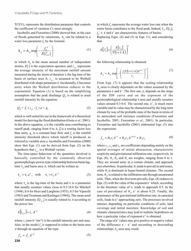
In a former application of the model to a large region ofSouthern Italy including Basilicata, Calabria and Puglia(Claps et al., 2001), the ratios of estimates of Λq and Λp

were compared for basins of Calabria (mostly humid andpermeable) and of Puglia and Basilicata (the arid ones).Figure 2 and Table 1 report the results of the analysis. Adifferent behaviour, not dependent on the basin area, isshown by the humid basins of Puglia and Basilicata, wherethe flood-rainfall yield in terms of number of events isbasically controlled by the climate.

Fig. 2. Mean annual number of flood and rainfall events ratio versusbasin area A in Calabria and arid basins in Puglia and Basilicata

Climatic control on the variability of flood distribution

233

The observed pattern of the ratio Λq/Λp can be explainedby means of Eqn. (7). In fact, the slope of the scaling Eqn.(4) of areal rainfall intensity is substantially homogeneousover the three regions and the resulting behaviour of theratio Λq/Λp depends on the scaling functions, Eqn. (5). InFig. 2 two slightly humid basins with large basin area(Ofanto at Rocchetta S. Antonio and Basento at Menzena),were also included.

The estimates of fA shown in Fig. 3 and Table 1 wereobtained by means of Eqn. (1) rearranged into:

[ ]( )

k

q

pAA k

iEf/1

log/11

ΛΛ

+Γ= (11)

As in Fig. 3a, in Calabria fA is almost constant (ε’=0). Somesignificant deviations from this behaviour may be observedin small basins (say below 50 km2) where local heterogeneitymay lead to consistent oscillations of the runoff threshold.In the figure, the horizontal line represents typical behaviourof humid basins where water losses do not scale with area.The constant value represented by the horizontal line is

considerably higher than that observed in humid basins ofBasilicata (Claps et al., 2001) where basins present similarclimatic indices. This may reflect the fact that basins inCalabria are characterised by higher mean permeabilitycompared to basins in Basilicata. In arid basins of Pugliaand Basilicata, a clear relationship of the type shown in Eqn.(5) is observed with, ε’=0.5.

Coefficient of variation of floods andbasin areaThe behaviour of the coefficient of variation Cv of annualfloods was investigated with particular regard to the way ittends to scale with the basin area A. According to theprobability distribution proposed by Iacobellis andFiorentino (2000), Cv is controlled mainly by the meanannual number of floods, Λq, and by the shape parameter ofthe probability distribution of rainfall, k. In the model, Λq isin turn dependent on Λp, fA and E[iA], whose definitions areprovided earlier. In the theoretical framework presentedabove, and in a region where k ad Λp are constant, parametersE[iA] and fA scale with the basin area by a power law withexponents ε and ε’ respectively. Therefore, following Eqn.(7), the relationship Cv-A depends on ε and ε’.

This result adds new arguments to the controversialquestion whether Cv should theoretically increase ordecrease as the basin size becomes larger. In fact, manyobserved datasets, reported in the literature, show a decreaseof Cv with area, usually ascribed to the limited spatial extentof extreme events that leads to a decrease of Cv of arealrainfall intensity. An increase of Cv with the area at smallscales is also often observed. Robinson and Sivapalan(1997a) associated this pattern with the interaction betweenrainfall and a catchment’s characteristic timescales whileBlöschl and Sivapalan (1997) indicated nonlinear runoffprocesses, controlled by thresholds, as the main mechanismsfor the increasing of Cv, while analysing the role of severalother different process controls.

The model proposed here suggests that a significant rolein the control of Cv is played by the abstractioncharacteristics (through the parameter fA) at the basin scale.In addition, this parameter has been shown to be stronglyrelated to the long-term climate which drives the scalingrelationship Cv-A. In particular, a double control isrecognized: one related to the precipitation IDFs and theirscaling with duration (through the model parameter ε); theother represented by the strong influence of the basinresponse in terms of the flood number ratio Λq / Λp asdetermined by the rainfall threshold fA for runoff generation.In other words, the presented theoretical framework allowsthe relationship between the coefficient of variation Cv of

Fig. 3. Average space-time water loss intensity versus basin area Ain Calabria (a) and arid basins in Puglia and Basilicata (b).

V. Iacobellis, P. Claps and M. Fiorentino

234

annual floods and the basin scale to be investigated by justlooking at the dependence of the parameters involved onbasin scale. For example, the ε value, representative of theprecipitation scaling patterns, shows a decreasing patternversus area, producing lower Cv at larger scales. This isdue to the effect of the areal averaging of precipitation andcan be reproduced by the application of the classic U.S.Weather Bureau areal reduction factor to a power-law IDF(see Eqn. (10)). The same effect was also recognized bySivapalan and Blöschl (1998), who derived a catchment’sIDF curves and related areal reduction factors based on thespatial correlation structure of rainfall.

As a first approximation, it can be assumed that k = 1,corresponding to the hypothesis of exponential distributionof rainfall intensity. In this case the proposed model leadsto a distribution that, under a wide range of situations, isnot very far from a simple Gumbel distribution (EV1).

The standard form of the Gumbel distribution’s cdf,written as

( )

αξ−−−= QQFq expexp (12)

with variance σ2q and mean µq values respectively

6

222 απ=σq

, α+ξ=µ 5771.0q (13)

can also be expressed as the distribution of the maximumof a Poissonian number of exponentially distributed peaksover a threshold x0 →0. In this case the form of the EV1appears as (Stedinger et al., 1992)

( )

−Λ−=

αQQF qq expexp (14)

where α is the mean of the exponential variable and Λq isthe rate of the Poisson process. Gumbel parameters α and ξcan be thus related to Λq through the moments (Eqn. (13))of the distribution, providing

( )qΛ= lnαξ . (15)

Then the following relation between Cv and Λq arises:

5771.0log28255.1

+Λ=

µσ

=qq

qCv(16)

In terms of the parameters of the proposed models, replacingEqn. (1) into (16) produces:

5771.0ln

28255.1'

1

1 +−Λ=

ε−εAif

Cvp

(17)

which represents the above-mentioned Cv-A relationship.In Fig. 4, as an example, the form assumed by therelationship of Eqn. (17) is shown for two different Poissonrates: Λp= 5 and Λp=20. The other parameter values assumedare i1 = 13 mm h-1 km0.66, ε = 0.33 and fA = 0.75 mm/h, forA=2500 km2. The patterns shown in Fig. 4 for differentvalues of ε’ (0, 0.16, 0.33 and 0.5) producing correspondingvalues of f1 (0.75, 2.6, 9.8 and 37 mm h-1 km2ε’), highlightthat the scaling relationship Cv-A, the other quantitiesconstant, is significantly dependent on the values ε and ε’and their difference.

Fig. 4. Coefficient of variation of flood annual maxima versus basinarea A, according to equation (17), with i1 = 13 mmh-1km0.66,ε = 0.33, variable f1 (mmh-1km2ε’) and ε’, and (a) Λp=5; (b) Λp=20.

Climatic control on the variability of flood distribution

235

Commenting on Fig. 4 and taking into account the typicalvalues of ε’ presented in the previous section, it is possibleto observe that Cv decreases with the basin area A in aridbasins, where the prevailing runoff generation mechanismis of the infiltration excess (Horton type) and fA tends toscale with A raised to the power ε’ = 0.5 (for a more generalcomment on this topic, see also Fiorentino and Iacobellis,2001). Conversely, in humid and vegetated basins, wherethe prevailing runoff generation mechanism is saturationexcess (Dunne type), and ε’ tends to zero, Cv may increaseas the basin area increases. On the other hand, Fig. 4 alsopoints out that Eqn. (17) shows a more significant sensitivityof Cv to A when ε’ is greater than ε. This may provide anexplanation for the fact that in the real world a negativescaling of Cv with the basin area A seems to prevail.

A relationship analogous to Eqn. (17) is derived in termsof L-moments (λ1, λ2, ...) and L-moment ratios, defined as(Hosking, 1990):

12 / λλτ = ; 2/ λλτ rr = ; r = 3, 4, ... (18)

The latter have meaning of coefficient of variation (L-cv),skewness (L-ca) and kurtosis (L-k) respectively: τ, τ3, τ4.

L-moments unbiased estimators are expressed by:

l p br r k kk

r

+=

= ∑10

,* with

( )( ) ( )( )( ) ( )b n

j j j kn n n k

xk jj

n

=− − −− − −

−

=∑1

1

1 21 2

...

...(19)

where xj, j = 1,...,n is the ordered finite sample and n is theobservation length; bk and lr are unbiased estimators of βk

and λr (βk are probability weighted moments introduced byGreenwood et al., 1979), while t=l2 / l1 and tr=lr / l2 areconsistent but not unbiased estimators of τ and τr.

Hence, Eqn. (15) is replaced by (Stedinger et al., 1992)

( )2ln2 α=λ (20)

and the following expression of L-Cv is obtained:

( )5771.0ln

2ln'

1

1 +−Λ=−

ε−εAif

CvLp

(21)

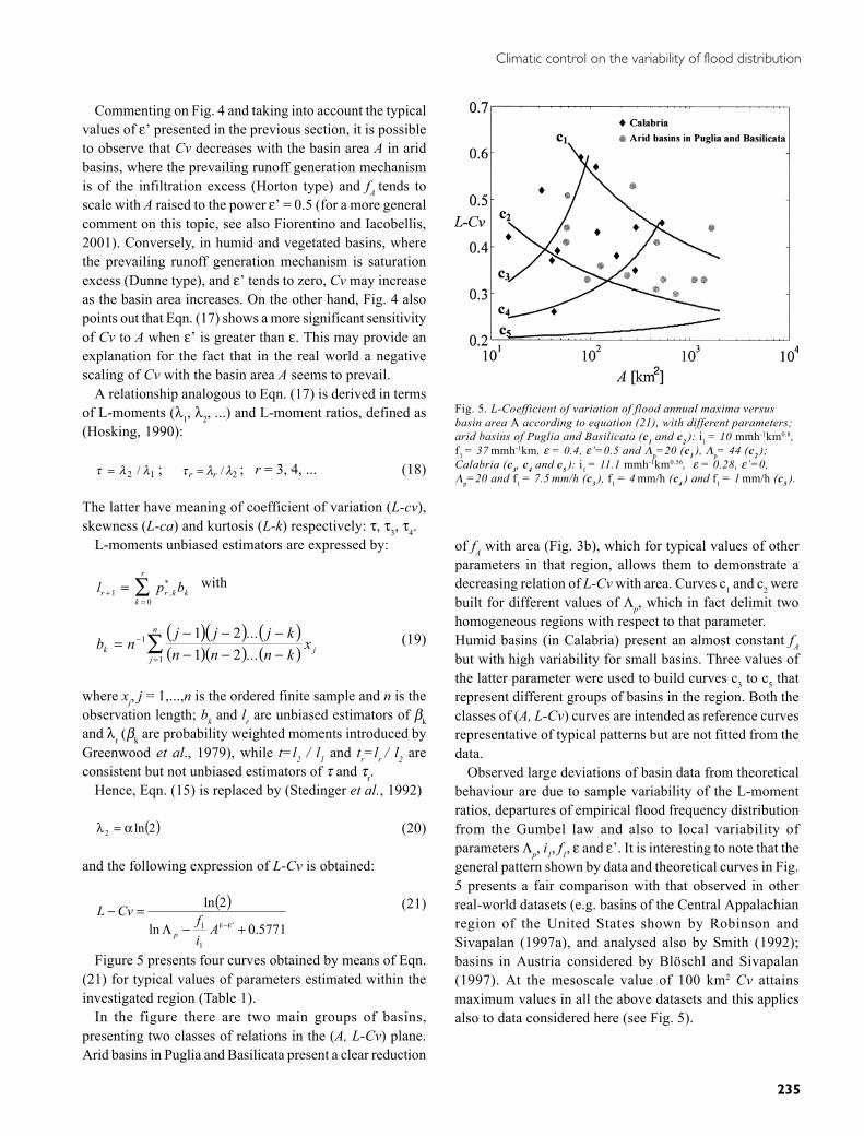
Figure 5 presents four curves obtained by means of Eqn.(21) for typical values of parameters estimated within theinvestigated region (Table 1).

In the figure there are two main groups of basins,presenting two classes of relations in the (A, L-Cv) plane.Arid basins in Puglia and Basilicata present a clear reduction

Fig. 5. L-Coefficient of variation of flood annual maxima versusbasin area A according to equation (21), with different parameters;arid basins of Puglia and Basilicata (c1 and c2 ): i1 = 10 mmh-1km0.8,f1 = 37 mmh-1km, ε = 0.4, ε’=0.5 and Λp=20 (c1 ), Λp= 44 (c2 );Calabria (c3, c4 and c5 ): i1 = 11.1 mmh-1km0.56, ε = 0.28, ε’=0,Λp=20 and f1 = 7.5 mm/h (c3 ), f1 = 4 mm/h (c4 ) and f1 = 1 mm/h (c5 ).

of fA with area (Fig. 3b), which for typical values of otherparameters in that region, allows them to demonstrate adecreasing relation of L-Cv with area. Curves c1 and c2 werebuilt for different values of Λp, which in fact delimit twohomogeneous regions with respect to that parameter.Humid basins (in Calabria) present an almost constant fA

but with high variability for small basins. Three values ofthe latter parameter were used to build curves c3 to c5 thatrepresent different groups of basins in the region. Both theclasses of (A, L-Cv) curves are intended as reference curvesrepresentative of typical patterns but are not fitted from thedata.

Observed large deviations of basin data from theoreticalbehaviour are due to sample variability of the L-momentratios, departures of empirical flood frequency distributionfrom the Gumbel law and also to local variability ofparameters Λp, i1, f1, ε and ε’. It is interesting to note that thegeneral pattern shown by data and theoretical curves in Fig.5 presents a fair comparison with that observed in otherreal-world datasets (e.g. basins of the Central Appalachianregion of the United States shown by Robinson andSivapalan (1997a), and analysed also by Smith (1992);basins in Austria considered by Blöschl and Sivapalan(1997). At the mesoscale value of 100 km2 Cv attainsmaximum values in all the above datasets and this appliesalso to data considered here (see Fig. 5).

V. Iacobellis, P. Claps and M. Fiorentino

236

ConclusionsIn this study the variability of the coefficient of variationCv of flood peaks annual maxima was investigated withparticular regard to the way it tends to scale with the basinarea A. The analysis was developed within the frameworkof the theoretical distribution of floods proposed byIacobellis and Fiorentino (2001). According to thisdistribution, Cv is controlled mainly by the mean annualnumber of floods, Λq and by the shape parameter k of the(PEV) probability distribution of rainfall. In the model, Λqis in turn dependent on parameters Λp, fA and E[iA]. In regionswhere k and Λp are constant, E[iA] and fA scale with the basinarea. Therefore, the relationship Cv-A depends on the scalingparameters ε and ε’ respectively related to the structure ofprecipitation and to a combination of soil and climateparameters. This result suggests that the Cv behaviour iscontrolled by the abstraction characteristics at the basinscale, as well as by long-term climate.

The decrease in Cv with area which is often observed, isreproduced correctly where the infiltration excess (Hortontype) mechanism dominates, as in arid and impermeablebasins, or whenever ε < ε’. On the other hand, an increaseof Cv with area can be justified in humid and vegetatedbasins and is consistent with saturation excess (Dunne type)runoff.

When examining real-world data, the sample variabilityof L-moments and of the model parameters can play amarked role, as well as the departure of the flood frequencydistribution from the EV1 model, which drives the Cv-Λq

relation.Finally, non-linear effects due to the superposition of

different mechanisms of runoff generation, which addcomplexity to the scaling properties of Cv, are not takeninto account in this paper.

AcknowledgementsThis work was supported by funds granted by the ConsiglioNazionale delle Ricerche – Gruppo Nazionale per la Difesadalle Catastrofi Idrogeologiche and by MURST (ItalianMinistry of Education and University), project ECAPI.Comments and suggestions of two anonymous reviewersare gratefully acknowledged.

ReferencesBlöschl, G. and Sivapalan, M., 1997. Process controls on regional

flood frequency: Coefficient of variation and basin scale, WaterResour. Res., 33, 2967–2980.

Claps P., Copertino, V.A., Ermini, R. and Fiorentino, M., 1994.Analisi regionale dei massimi annuali delle precipitazioni didiversa durata (in Italian). In: Valutazione delle piene in Pugliareport, Dipartimento di Ingegneria e Fisica dell’Ambiente andGruppo Nazionale per la Difesa dalle Catastrofi Idrogeologiche,Univ. della Basilicata, Potenza, Italy.

Claps, P., Fiorentino, M. and Iacobellis, V., 2001. Regional floodfrequency analysis with a theoretically derived distributionfunction, Proc. of the 2nd Plinius Conference on MediterraneanStorms, European Geophysical Society, Siena, Italy, 16–18October 2000 (in press),

DIFA, 1998. Valutazione delle Piene in Basilicata (in Italian),report, Dipartimento di Ingegneria e Fisica dell’Ambiente andGruppo Nazionale per la Difesa dalle Catastrofi Idrogeologiche,Univ. della Basilicata, Potenza, Italy.

Eagleson, P.S., 1972. Dynamics of flood frequency, Water Resour.Res., 8, 878–898.

Ermini, R. and Fiorentino, M., 1994. I tempi di ritardo caratteristicidei bacini idrografici. In: Valutazione delle Piene in Puglia,report, Dipar-timento di Ing. e Fis. dell’Ambiente, Univ. dellaBasilicata, Potenza, Italy.

Fiorentino, M. and Iacobellis, V., 2001. New insights about theclimatic and geologic control on the probability distribution offloods. Water Resour. Res., 37, 721–730.

Fiorentino, M., Gabriele, S., Rossi, F. and Versace, P., 1987.Hierarchical approach for regional flood frequency analysis.In: Regional flood frequency analysis, V.P. Singh (Ed.), D.Reidel, Norwell, MA., 35–49.

Fiorentino, M., Margiotta, M.R. and Iacobellis, V., 2001. Effectsof Climate and Antecedent Soil Moisture on the Areal AverageAbstraction Losses. Proc. XXIX IAHR Congress, September 16-21, 2001.

Gabriele, S. and Iiritano, G., 1994. Alcuni aspetti teorici edapplicativi nella regionalizzazione delle piogge con il modelloTCEV, (in Italian), GNDCI – Linea 1 U.O. 1.4, PubblicazioneN. 1089, Rende (Cs).

Gioia, G., Iacobellis,V. and Margiotta, M.R., 2001. Assessmentof a simplified runoff model for the theoretical derivation ofthe probability distribution of floods. In: The Extremes of theExtremes: Extraordinary Floods, Arni Snorrason et al. (Eds.)IAHS Publ. no. 271.

Greenwood, J.A.,Landwehr, J.M., Matalas, N.C. and Wallis, J.R.,1979. Probability weighted moments: Definition and relationto parameters of several distributions expressable in inverseform. Water Resour. Res., 15, 1049–1054.

Gupta, V. K. and Dawdy, D.R., 1995. Physical interpretations ofregional variations in the scaling exponents of flood quantiles,Hydrol. Process., 9, 347–361.

Hosking, J.R.M., 1990. L-moments: Analysis and estimation ofdistributions using linear combinations of order statistics, J. Roy.Stat. Soc., B 52, 105–124.

Hosking, J.R.M. and Wallis, J.R., 1993. Some Statistic useful inRegional Frequency Analysis, Water Resour. Res., 29, 271–281.

Hoyt, W.G. and Langbein, W.B., 1955. Floods. PrincetonUniversity Press, NJ. 469 pp.

Iacobellis, V. and Fiorentino, M., 2000. Derived distribution offloods based on the concept of partial area coverage with aclimatic appeal. Water Resour. Res., 36, 469–482.

Iacobellis, V., Claps, P. and Fiorentino, M., 1998. Sulla dipendenzadal clima dei parametri della distribuzione di probabilità dellepiene, (in Italian), In: Proc. XIV Convegno di Idraulica eCostruzioni Idrauliche, Univ. of Catania, Catania, Italy. II, 213–224.

Mitchell, W.D., 1948. Unit hydrographs in Illinois. Dept. PublicWorks and Buildings, Division of Waterways, Illinois. 294 pp.

Climatic control on the variability of flood distribution

237

Robinson, J.S. and Sivapalan, M., 1997a. An investigation intothe physical causes of scaling and heterogeneity of regionalflood frequency. Water Resour. Res., 33, 1045–1059

Robinson, J.S. and Sivapalan, M., 1997b. Temporal scales andhydrological regimes: Implications for flood frequency scaling.Water Resour. Res., 33, 2981–2999.

Rossi, F., 1974. Criteri di similitudine idrologica per la stima dellaportata al colmo di piena corrispondente ad un assegnato periododi ritorno. Paper presented at the XIV Convegno di Idraulica eCostruzioni Idrauliche, Univ. of Naples, Naples, Italy.

Rossi, F., Fiorentino, M. and Versace, P., 1984. Two componentextreme value distribution for flood frequency analysis. WaterResour. Res., 20, 847–856.

Sivapalan, M. and Blöschl, G., 1998. Transformation of pointrainfall to areal rainfall: Intensity-duration-frequency curves.J. Hydrol., 204, 150–167.

SIVAPI, 1999. Sistema Informativo per la Valutazione delle pienein Italia. (http://www.gndci.cs.cnr.it./sivapi).

Smith, J.A., 1992. Representation of basin scale in flood peakdistributions. Water Resour. Res., 28, 2993–-2999.

Stedinger, J.R., Vogel, R.M. and Foufoula-Georgiou, E., 1992.Frequency analysis of extreme events. In: Handbook ofHydrology, D.R. Maidment (Ed.), Chap. 18, McGraw-Hill.

Thornthwaite, C.W., 1948. An approach toward a rationalclassification of climate. Amer. Geograph. Rev., 38, 55–94.

Troutman, B.M. and Karlinger, M.R., 1984. Unit hydrographapproximations assuming linear flow through topologicallyrandom channel networks. Water Resour. Res., 21, 743–754.

Turc, L., 1961. Estimation of irrigation water requirements,potential evapotranspiration: a simple climatic formula evolvedup to date. Ann. Agronomy, 12, 13–14.

Versace, P., Ferrari, E., Gabriele, S. and Rossi, F., 1989.Valutazionedelle piene in Calabria (in Italian). CNR-IRPI, Geodata.

Villani, P., 1993. Extreme flood estimation using Power ExtremeValue (PEV) distribution. Proc. IASTED International Conf.,Modeling and Simulation, M.H. Hamza (Ed.), Univ. ofPittsburgh, Pittsburgh, PA. 470–476.

Viparelli, C., 1963. Ricostruzione dell’idrogramma di piena (inItalian). L’Energia Elettrica, No. 6, 421–428.

V. Iacobellis, P. Claps and M. Fiorentino

238