17B.5

WORLDWIDE MICROPHYSICAL THUNDERSTORM VARIABILITY

IN DIFFERENT CLIMATIC REGIONS: A THREE-DIMENSIONAL CLOUD MODELING STUDY

Robert E. Schlesinger, Shane A. Hubbard and Pao K. Wang

Department of Atmospheric and Oceanic Sciences University of Wisconsin – Madison

Madison, Wisconsin 53706 USA

1. INTRODUCTION An evolving research group at the University of Wisconsin, led by third author Wang, has for two decades been studying the microphysical structure of thunderstorms as documented in Straka (1989), Johnson et al. (1993, 1994), Lin and Wang (1997), Lin et al. (2005; henceforth LWS05) and Schlesinger et al. (2006; henceforth SHW06). The key tool has been a three-dimensional (3D) cloud model known as WISCDYMM (the Wisconsin Dynamical and Microphysical Model), originated by Straka (1989), subsequently modified by the research group (Johnson et al. 1993, 1994; Lin and Wang 1997; LWS05; SHW06), and summarized briefly in section 2. However, all these previous case studies prior to SHW06 were limited to summertime thunderstorms in two climatic regions, the U. S. High Plains and the humid subtropics. Straka (1989) simulated a Colorado multicell storm, Johnson et al. (1993, 1994) analyzed the impact of ice microphysics on a Montana supercell, and Lin and Wang (1997) simulated a multicell storm in Taipei, Taiwan. By means of six 2-h WISCDYMM simulations, LWS05 compared the microphysical aspects of three thunderstorms apiece in the High Plains (the Colorado and Montana cases plus a North Dakota storm) and the humid subtropics (the Taipei storm and two south Florida cases). Despite being limited to only two climatic regions and the summer months, LWS05 yielded two notable findings: a) Throughout the active life of a given storm after its early adjustment phases, the fraction of the total condensate mass contributed by each hydrometeor type seemed to be quasi-steady, along with the individual microphysical transfer rates contributing to the production and depletion of each precipitating hydrometeor category; and ____________________________________________ *Corresponding author address: Robert E. Schlesinger, Department of Atmospheric and Oceanic Sciences, University of Wisconsin - Madison, Madison, Wisconsin, 53706; e-mail: schlesin@meteor.wisc.edu.

b) The partitioning broke down differently in one geographic region versus the other. The High Plains storms had much higher frozen condensate mass fractions than the subtropical storms, ~0.78-0.82 versus ~0.48-0.57. Since the simulated storm structures were found to compare favorably with observations (LWS05), it is quite plausible to regard them as physically realistic. The above findings motivated us to embark on a subsequent WISCDYMM-based thunderstorm variability study that retains much the same overall spirit as in LWS05, but is far larger in scope and also more closely oriented toward thunderstorm variability in relation to severe local storm environment indices including CAPE (Convective Available Potential Energy) and Total Totals. In final form, this expanded study, subsumes 105 thunderstorm cases distributed among 10 climatic zones, including a sizable minority of cases from seasons other than summer. This substantially wider variety of storm cases versus LWS05, of which an earlier stage with 56 cases distributed among the same 10 climatic zones was reported in SHW06, has been compiled in order to investigate whether systematic differences in the bulk microphysics of simulated storms in contrasting climatic regions continue to apply when the variety of thunderstorm-supporting environments is thus broadened. This paper highlights some of our finalized results. 2. EXPERIMENTAL CONDITIONS 2.1 Model Properties WISCDYMM is a time-dependent nonhydrostatic quasi-compressible 3D model in standard Cartesian coordinates. The model domain is 55x55x20 km3 in the respective x-, y- and z-coordinates, with 55x55x100 grid cells of dimensions 1.0x1.0x0.2 km3. Finite-difference advection schemes and boundary conditions are as in LWS05, with subgrid flux parameterizations as in Straka (1989). Radiation, topography and the Coriolis force are omitted. The time step is 2 s, with a reduced sound speed of 200 m s-1.

Predicted model fields are the three wind components, potential temperature, pressure, water vapor mixing ratio, and the mixing ratios for five classes of hydrometeors: cloud water, cloud ice, rain, snow and graupel/hail. The microphysical package features a bulk parameterization which, as elaborated in Straka (1989), is based mainly on Lin et al. (1983) and Cotton et al. (1982, 1986). Cloud water droplets and cloud ice crystals are monodisperse and move with the air, while precipitating hydrometeors follow inverse exponential size distributions. The bulk microphysics parameterization provides for up to 37 mass transfer rates among water substance classes. Several of these rates (e.g., condensation onto and evaporation from wet snow and wet graupel/hail) are turned off in the simulations reported herein. As itemized in Table 1 of SHW06, 25 of the active transfer rates are a source or sink of precipitation. 2.2 Initialization As in Klemp and Wilhelmson (1978), convection in WISCDYMM is initiated by a quasi-ellipsoidal buoyant bubble in the lower central portion of the domain, superimposed on a horizontally homogeneous hydrostatic base state. In each case, the base-state potential temperature, water vapor mixing ratio and horizontal wind components are computed by vertically interpolating the respective temperature, dew point and horizontal wind components from the closest available sufficiently deep rawinsounding in space and time on the University of Wyoming's sounding archive website http://weather.uwyo.edu/upperair/sounding.html to the model grid levels, deriving the pressure profile via upward integration of the hydrostatic equation starting from the surface pressure in the sounding. If in a given case WISCDYMM produces a storm that dissipates unrealistically early, such as a single short-lived (~1 h or less) cell in a situation where a multicell system lasting 2 h or longer occurred, the lowest few kilometers of the base state from the interpolated raw sounding may contain insufficient moisture and/or too strong a cap to truly represent the actual near environment of the observed storm. In such instances, prior to imposing the buoyant bubble, the vertical temperature and mixing ratio profiles in the interpolated sounding are preconditioned to suitably increase the relative humidities and/or weaken the cap by imposing a time-independent parabolic lifting profile for 1, 2 or at most 3 h throughout the layer to be occupied by the impulse, keeping the wind profile unchanged. The pressure profile in the lifted layer is updated by integrating hydrostatically downward from its top to the surface

Further details concerning the model initialization procedure are given in SHW06. These include the dimensions and amplitude of the buoyant bubble, the depth and amplitude of the lifting profile, and our method of taking the latent heat of fusion into account at temperatures colder than 0˚C. 2.3 Run-Time Strategy Each WISCDYMM simulation is run out to 120 min (2 h), restarting every 20 min while saving the model fields and auxiliary microphysical data every 2 min. During any one 20-min segment, the domain is translated at a constant velocity relative to the earth so as to aim the most interesting convective cell for an ending position near the center of the domain area. The translation velocity generally varies among segments, and a segment is rerun if the first attempt ends with the cell of interest insufficiently well centered. 2.4 Range of Climatic Regions Sampled This study encompasses 105 WISCDYMM storm simulations initialized with University of Wyoming archive rawinsoundings from 79 stations in various parts of the world. Of these locations, plotted herein on a global map (Fig. 1), 62 entail one case each and the remaining 17 entail from two to four cases each. About two-thirds of the storm cases are from the United States east of the Rockies (41 cases, 27 locations), Europe west of 20˚E (16 cases, 14 stations) or Asia east of 80˚E (15 cases, 11 stations), but there is also a more limited sampling from other regions such as Canada, Australia

�������and Russia. Table 1 lists the 79 sounding locations by city and state (or country, if other than the United States), call symbol, latitude, longitude and elevation. The stations are grouped by each of 10 climatic zones, adapting a worldwide climatic classification map in Moran and Morgan (1994). We have subjectively subdivided their "temperate continental" classification into "warm summer" and "cool summer" subtypes. Despite being located as far north as southern Minnesota, some midlatitude European stations such as Nimes (France) and S Pietro di Capofiume (Italy) with dry summers were evidently considered to be subtropical in Moran and Morgan (1994) because their winters are mild for their latitudes. We have used the common synonym “Mediterranean” to label their climate type. The “High Plains” descriptor in LWS05 is not among the climatic classifications in Moran and Morgan (1994). Nevertheless, we regard five of the extratropical stations, encompassing seven of the storm cases, as having High Plains characteristics because they occurred at semi-arid locations with surface elevations greater than 700 m MSL. This applies to five cases among four dry/steppe stations and two cases at one boreal station, symbolized in Table 1 by suffixing the climatic descriptors for those five stations with “HP”.

Table 2 displays the numerical partitioning of the 79 stations and 105 cases among the 10 climate zones. Clear majorities of both counts, 54 and 77 respectively, are distributed among four of the zones: warm-summer temperate continental, humid subtropical, Meditterranean and humid tropical, each of the remaining six zones being much more sparsely represented. This admittedly uneven distribution is a consequence of both a mostly lower thunderstorm frequency and a sparser sampling of those zones among the worldwide rawinsonde stations in the University of Wyoming archive. In LWS05, all six storm cases occurred in the Northern Hemisphere and were confined to the summer months of June through August. In our current 105-case study, by contrast, excluding three cases within 10˚ of the equator and hence nearly devoid of thermal seasonality, 38 Northern Hemisphere cases occurred outside of the warm months, defined for our purposes as May through September. Also, another 10 of our cases occurred in the Southern Hemisphere, though all of those 10 cases were confined to the corresponding warm months of November through March. Finally, a brief explanation of our nomenclature for the WISCDYMM thunderstorm simulations is in order. We use a symbolic case name that embodies the location, date and time of the associated University of Wyoming archive sounding along with the duration of lifting applied to its interpolated counterpart prior to imposing the initial buoyant impulse. We start with the station call symbol (Table 1) and continue with the year, month, hour and finally the number of hours over which lifting is applied, e.g., 11722-020716-12+2h for Brno, Czech Republic on 16 July 2002 at 1200 UTC with 2 h of lifting, or BNA-980416-18+0h for Nashville, TN on 16 April 1998 with no lifting. 2.5 Case Selection Methodology No single method was used to select the storms in this extensive study. In many instances, the nearest available archived University of Wyoming rawinsounding in space and time to an observed deep convective cell or system was determined from infrared signatures of convective cloud tops, i.e., conspicuous cold spots, in satellite imagery loops from the Space Science and Engineering Center at the University of Wisconsin-Madison. In other cases, the sounding was chosen on the basis of prior knowledge about the time and location of widely known thunderstorm and/or severe weather cases such as the Alabama tornadic supercells on the evening of 8 April 1998 or the Illinois tornado outbreak of 19 April 1996, or on the basis of information obtained by Googling the web, e.g., one mid-spring Virginia storm case (IAD-940501-00+1h) was found by Googling for sites containing such telltale words or phrases as “low-topped” and “supercell”. In some of the cases, corroborating documentation of actual storm activity at the selected station could be found from surface observations archived at the worldwide weather web link

http://www.wunderground.com/ Due to the crude spatial and temporal resolution of the rawinsonde network versus the scales of the WISCDYMM simulations, the nearest storm activity missed the station in some cases, but by a small enough margin to uphold the suitability of the sounding as a proximity profile, aside from the potential representativeness issues broached in section 2.2. 3. RESULTS The following three considerations figure strongly into our coverage of the WISCDYMM storm simulation results: 1) As in LWS05, we evaluate and intercompare the broad microphysical makeup of our simulated storms by computing time-averaged masses for the five individual hydrometeor (condensate) classes over a large part of the mature storm stage, 60-120 min in all our experiments, then dividing each by the total condensate mass time-averaged over the same period. The bulk hydrometeor mass fractions thus defined pertain to cloud water (CWF), cloud ice (CIF), rain (RF), snow (SF) and hail (HF). More briefly, we also touch upon bulk storm dynamics via the maximum updraft velocity WMAX or maximum updraft kinetic energy KE = (WMAX)2/2 during the same period. We have chosen this time interval because it spans a substantial fraction (50%) of the total simulation time and also begins long after the early (~15 min) bubble-induced overshooting updraft peak that occurs in most of the cases. 2) We also refer extensively to one of five other bulk hydrometeor mass fractions derived from the five primary indices in LWS05. This derived quantity is the total frozen hydrometeor fraction, or “ice fraction” (IF) for brevity’s sake, and is defined by IF = CIF + SF + HF. 3) Because a large minority of our simulated cases occurred outside of the warm months as noted in section 2.4, we compare our results for the warm-month subset of 64 cases versus the full set of 105 to gauge whether or not the results are significantly influenced by the inclusion of the cool-month storms in the full mix. 3.1 Utilization of CAPE Scattergrams of KE versus CAPE, superimposing the least-squares regression lines as well as their equations and correlation coefficients, are plotted in Fig. 2 for all 105 storm cases (left panel) and the subset of 64 warm-month cases (right panel). Using the relationship WMAX = (2*KE)1/2, Fig. 3 plots the corresponding scattergrams of WMAX versus CAPE. The superimposed blue curves in Fig. 3 represent the WMAX values derived from the least-squares regression lines for KE versus CAPE in Fig. 2.

Due to the scatter in these plots, the highest values of CAPE and KE (or WMAX) occur in different experiments, and likewise for the lowest values of those two parameters. Among all 105 cases, CAPE varied from 733 J kg-1 for a central Tennessee case (BNA-051116-00+1h) to 7226 J kg-1 for an east Indian case (VECC-050410-12+1h), whereas KE (WMAX) varied from 118 J kg-1 (15.36 m s-1) for a Malaysian case (WSSS-000918-09+00h) to 3279 J kg-1 (80.98 m s-1) for a northeast Texas case (FWD-060510-00+0h), While qualitatively similar on the whole, the scattergrams in Figs. 2 and 3 do show somewhat better utilization of CAPE by the 60-120 min peak updraft among the warm-month cases than among all cases, with WMAX typically ~61% versus ~53% of the upper bound from parcel theory, judging from the square root of the coefficient for CAPE in each regression equation for KE. The positive correlation between KE and CAPE, already rather strong among all cases (+0.750), is even better among the warm-month cases (+0.844). 3.2 Effects of Climate Zone and Season on Ice

Fraction Figure 4 plots the distributions of the ice fraction IF for the four best-sampled climate zones from Table 2 as well as for the “High Plains” cases from the dry/steppe and boreal zones, encompassing 84 cases from the full set of 105 (left panel) and 47 cases from the warm-month subset of 64 (right panel). Also shown in Fig. 4, just above the abscissas, are the mean IF values and case counts for each of the five zones. Despite the sparser sampling of each climate type for the warm-month versus full sets of cases, especially for the humid subtropics and humid tropics, both panels offer quantitatively similar findings to each other with regard to IF, differing only in details: 1) Unlike in LWS05, our far wider study shows wide intrazonal variability and extensive interzonal overlap among all four of the best-sampled climate zones. In both panels, the intrazonal range of IF for each of those zones amounts to well over half the difference between the largest IF value among all 105 cases, 0.8028 for a midsummer Colorado case (DNR-960714-00+2h) and the smallest, 0.1998 for a midsummer east Indian case (VECC-000722-00+0h). Being summertime occurrences, both of those extreme cases are included in both panels, in the “High Plains” and humid tropical zones respectively. 2) The similarly large spreads of individual IF values in each climate zone in Fig. 4 other than “High Plains”, both with and without inclusion of cases from the climatologically cooler months, suggests strongly that the type of airmass visiting a climate zone on a storm day is of comparable importance to which zone the airmass is visiting. This surmise is at least plausible, considering that extratropical cool-month thunderstorms, or for that matter warm-month thunderstorms at high-

latitude locations with cool summers, are favored by the presence of unseasonably warm and/or moist air throughout lower levels as opposed to a climatologically typical environment. In retrospect, the wide separation of IF ranges between the humid subtropical and High Plains storm simulations of LWS05 may have been, at least in part, a fortuitous consequence of the very small sample sizes. 3) There is little to choose among the three mean IF values for the warm-summer temperate continental, humid subtropical and Mediterranean cases in either set, as all six of those mean values fall between 0.58 and 0.65 with spreads of barely 0.06 among the 58 applicable cases in the left panel and less than 0.03 among the 34 applicable cases in the right panel. 4) The mean IF values for our “High Plains” versus humid subtropical cases fall, to within a small margin (< 0.015) of 0.7 and 0.6 in the respective left and right panels. Hence, the mean IF in the “High Plains” storms exceeds that of the humid subtropical storms by margins on the order of 0.10 (0.1263 and 0.0856 in the respective left and right panels). However, these margins are less than half as large as among the three summertime storms apiece from the same zones in LWS05, which showed mean IF values of ~0.80 and ~0.54 and hence a margin of ~0.26. 5) Our “High Plains” versus humid tropical cases show by far the largest interzonal difference for the mean IF, slightly better than 0.25 between averages that fall close to 0.7 and 0.45 respectively. Moreover, there is very little overlap between the two distributions for the larger set of cases (left panel) and none for the smaller set (right panel). 3.3 Overall Thunderstorm Morphologies Our extensive set of WISCDYMM-based worldwide thunderstorm simulations produced a variety of morphological storm structures during maturity, on the basis of northward-looking pseudo-3D Tecplot animations of the approximate cloud boundary over the 2-h simulation time with 2-min frame resolution. As in SHW06, we equated the cloud boundary empirically with the 90% isosurface of relative humidity with respect to ice. Of the 105 simulated storms: 1) Fifty-four were multicellular, with one or more new cells developing after the bubble-induced initial cell had matured. Of these 54 storms, 29 were backbuilding (new cells developing preferentially upshear of previous ones, relative to the deep tropospheric mean shear vector) and the other 25 were complex (no preferred flank for new cells). 2) Thirty-one appeared supercellular. Nine of these 31 showed no sign of splitting, although three evolved into backbuilding multicellular mode toward the end of the simulation period. The other 22 appeared to

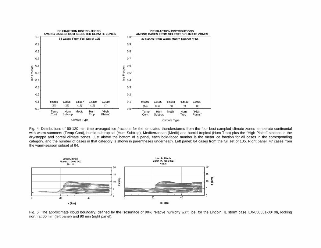
split, although 11 of those became multicellular late, nine backbuilding and the remaining two complex. 3) The mode of the remaining 20 storms could not be firmly determined from the Tecplot animations. That, and the word “appeared” in point 2, reflect uncertainties inherent in viewing the animations, most notably the potential for new cells developing behind, i.e., “into the screen” relative to, the visible part of the cloud boundary and going unobserved due to this obstructive effect. Accordingly, the ostensibly high supercell count in point 2 may well be an overestimate. 3.4 Contrasting Bulk Microphysics for Morphologically Similar Storms in Contrasting Air Masses: Two Examples The Tecplot animations revealed that storms developing in dissimilar air masses (base-state environments) could have broadly similar morphological structures despite highly contrasting hydrometeor mass fraction partitionings, even within one day at the same location. To illustrate this, we consider in this subsection two examples, of which the first involves two splitting supercells in different locations and seasons and the second involves two backbuilding multicellular storms about half a day apart at one location. The two splitting supercells are an early-spring Illinois case (ILX-050331-00+0h) and a midsummer Turkish case (17062-040729-12+2h). The two backbuilding multicellular storms are early-autumn north Italian cases late at night (LIML 061004-00+3h) and the following afternoon at the same location (LIML 061004-12+2h). Assorted environmental parameters from the interpolated University of Wyoming archive soundings for these four cases, after any applicable lifting, are displayed in Table 3 along with their symbolic case names. These parameters are surface elevation ZSFC, surface pressure PSFC, surface temperature TSFC, mean boundary-layer water vapor mixing ratio QVBL, lifting condensation level LCL, convective available potential energy CAPE, convective inhibition CIN, bulk Richardson number BRN, lifted index LI, Total Totals index TT, and melting level ZMLT. ZSFC and TSFC are taken unchanged from the raw archived sounding, as well as PSFC for input to the lifting preprocessor (if used). In Table 3, however, PSFC and all subsequent parameters pertain to their preprocessed counterparts on the WISCDYMM grid, i.e., after lifting (if any). Parameters QVBL through TT are computed the same way as in the archive except for CAPE, whose calculation ignores latent heat of fusion in the archive but takes it into account in our study, resulting in higher CAPE by typical margins of ~30-50%. For the same four storm cases, Table 4 lists the 60-120 min peak updraft WMAX along with the five individual hydrometeor mass fractions (CIF, HF, SF,

CWF, RF) and the ice fraction IF (the sum of CIF, HF and SF). Snapshots of these four storms are provided in Figs. 5-8, which show two frames apiece from the relevant Tecplot animations at 60 min (left panels) and 90 min (right panels). The splitting supercellular morphology of case ILX-050331-00+0h (Fig. 5) and especially case 17062-040729-12+2h (Fig. 6) is evident, as is the backbuilding (southwest flank) multicellularity of cases LIML-061004-00+3h (Fig. 7) and LIML-061004-12+2h (Fig. 8), although less dramatically than in the full animations. It is clear from Table 3 that the two splitting supercells in Figs. 5-6 evolved in highly contrasting air masses. In comparison with the environment of the Midwestern early spring storm ILX-050331-00+0h, that of the Turkish midsummer storm 17062-040729-12+2h was over 8 C˚ warmer at the surface with over 50% more moisture in the boundary layer and a far higher melting level. Somewhat ironically, despite comparable moderate CAPE in both environments, both LI and especially TT indicated less instability in case 17062-040729-12+2 than in case ILX-050331-00+0h, mainly because the 500-mb temperature (not tabulated) was nearly 10 C˚ warmer. As dramatized in Table 4, IF was far lower, ~0.53 versus ~0.78 despite a peak updraft ~25% stronger, and all three individual ice class mass fractions (CIF, SF, HF) were also substantially lower while the mass fractions for cloud water (CWF) and especially rain (RF) were higher. Apparently, the much warmer midlevels and higher melting level limited the ice mass fraction far more than the modestly stronger updraft enhanced it. Table 3 also shows that of the two early-autumn multicellular storms at the same north Italian location less than a day apart, the afternoon case LIML-061004-12+2h (Fig. 8) occurred in a considerably different environment than its predecessor LIML-061004-00+3h the night before (Fig. 7) as strong midlevel cold advection lowered the 500-mb temperature (not tabulated) by ~6.5 C˚ in connection with the passage of a trough (not shown). In Table 3, despite a ~20% boundary layer drying and a ~70% higher LCL, both LI and TT indicate dramatic destabilization. So does CAPE, which increased by ~50%, driving a comparable increase in WMAX, and the melting level lowered by 280 m despite a net surface warming of 3.4 C˚. Not surprisingly, as Table 4 clearly attests, IF also increased dramatically, from ~0.48 to ~0.73, and all three individual ice class mass fractions also increased substantially while both liquid mass fractions were roughly halved. This example corroborates the assertion in section 3.2 that the type of airmass visiting a climate zone (Mediterranean in this case) may be as important a modulator of bulk thunderstorm microphysics as which zone it is visiting. 3.5 Correlations Between Hydrometeor Mass

Fractions and Selected Environmental Indices

Once all our WISCDYMM-based worldwide thunderstorm simulations were completed and postprocessed, this study centered heavily around investigating the usefulness of various environmental indices as predictors of the hydrometeor mass fractions defined earlier, using as our utility criterion the correlation coefficients obtained from least-squares regression analysis. These correlation coefficients are tabulated in Table 5 for all 105 cases, and in Table 6 for the 64 warm-month cases to gauge the impact of omitting the cool-month cases from the sample space. The correlation coefficients in Tables 5 and 6 are for each hydrometeor mass fraction as a predictand, versus the following predictors: 1) The ground-relative melting level ZMLT; 2) ZMLT and CAPE, jointly; 3) The Total Totals index TT; 4) The 500-mb temperature T500, one of the parameters that figures into TT; 5) The Vertical Totals index VT = T850 – T500, one of the two summands comprising TT, where T850 is the 850-mb temperature; 6) The Cross Totals index CT = Td850 – T500, the other of the summands comprising TT, where Td850 is the 850-mb dew point; 7) The Significant Severe Parameter SSP, a composite index defined by Craven and Brooks (2004) by the product of CAPE and the magnitude of the 0-6 km AGL net wind shear vector. All of our least-squares fits were regression lines versus a single predictor (univariate) except under point 2, which entailed regression planes versus two predictors (bivariate). Note that multivariate correlation coefficients, unlike univariate ones, can be assigned only magnitude and no sign (positive-definite by default). Also, the two cases with the highest surface elevations, the midsummer Colorado case mentioned in section 3.2 (DNR-960714-00+2h) at 1625 m MSL and a late-spring South African case (FAIR-061121-09+1h) at 1523 m MSL, had surface pressures < 850 mb, so that none of TT, VT or CT could be defined, rendering T500 moot as a predictor. Hence, those two cases were excluded from both the full and warm-month sample spaces for TT and its components. For the full set of 105 cases (103 for TT or a component thereof as predictor), the following key findings may be gleaned from Table 5: 1) In the univariate analyses, the frozen hydrometeor mass fractions correlate negatively and the liquid hydrometeor mass fractions positively versus

ZMLT and T500. The opposite is true versus TT, VT, CT and SSP, except that there is no detectable correlation between the snow fraction and SSP. 2) Versus ZMLT, both cloud ice and total ice fractions show fair correlations approaching -0.5, the rain fraction a somewhat stronger correlation (~0.6) that makes it the best of the predictors, the hail and snow fractions slightly weaker correlations near -0,4, and cloud water only a marginal correlation. 3) Jointly versus ZMLT and CAPE, in comparison with the situation versus ZMLT alone, all the correlation magnitudes are improved, substantially so for all the frozen fractions except snow, for which the improvement is marginal; dramatically so for cloud water; and less markedly for rain, which nevertheless posts a rather strong bivariate correlation > 0.7. 4) Versus TT, all mass fractions except snow show far stronger correlations than versus ZMLT, approaching +0.8 for the total ice and hail fractions and only modestly less for cloud ice, close to -0,8 for rain, and ~ -0.6 for cloud water. 5) In comparison with the situation versus TT, all correlations are very similar versus VT but are ~35-50% weaker versus CT and also weaker by similar percentage ranges versus T500 except for snow. 6) Versus SSP, the mass fractions correlate less well overall than versus any of the predictors under points 2 through 5. None exceed ~0.45 in magnitude, most notably for the snow fraction, which has no detectable correlation with SSP. With regard to the bivariate linear regression versus ZMLT and CAPE, one other finding. not apparent from Table 5, is that each mass fraction varied versus CAPE in the opposite sense of its variation versus ZMLT on its least-squares plane (not shown), i.e., the frozen fractions decreased with increasing ZMLT and increased with increasing CAPE, and vice versa for the liquid fractions. For the 64 warm-month cases (62 for TT or a component thereof as predictor), Table 6 shows correlation coefficients quite similar to those for the full set in Table 5, indicating that omitting the cool-season storms from the sample space has only modest impact. The correlations show no systematic changes versus ZMLT or especially versus TT (or its components), slight improvement versus ZMLT and CAPE jointly for hail and cloud water, and modest improvement versus SSP for all fractions other than snow, enough to boost the correlation magnitudes for hail and cloud water to slightly over 0.5. Interestingly, linear regression analysis of the dynamic storm parameter WMAX versus SSP yielded considerably better correlations than did any of the hydrometeor mass fractions in Tables 5 and 6, as

demonstrated by Fig. 9. The correlation coefficient was +0.618 using all 105 storm cases, and slightly better yet at +0.687 using the 64-case warm-month subset, for which the upward slope of the regression line was also ~15% steeper. Still, there was sufficient scatter that the storm with the lowest value of SSP (3,626 m3 s-3), a late-summer Argentinian case (SARE-070305-12Z+2h), had a large WMAX value (46.52 m s-1) while the storm with the smallest WMAX (15.36 m s-1), the Malaysian case WSSS-000918-09+0h, had a much larger SSP value (17,925 m3 s-3). Both panels of Fig. 9 contain a significant minority of cases with SSP values well in excess of the 90th percentile of ~78,000 m3 s-3 among the 60,090 observed prestorm soundings analyzed in Craven and Brooks (2004); these very large SSP values are a consequence of the enhanced CAPE values resulting from our taking the latent heat of fusion into account for parcel temperatures colder than 0˚C. 3.6 Precipitation Source/Sink Rankings The six summertime thunderstorm simulations reported by LWS05 showed consistently different rankings among some of the most important sources and sinks of precipitation in their U.S. High Plains cases than in their humid subtropical cases. The #1 and #2 rain sources and hail sinks in all three of their High Plains storms were melting of hail and shedding from (wet) hail respectively, whereas the reverse was true for all three of their humid subtropical storms. Among hail sources, accretion of rain ranked #3 in two High Plains storms and #2 in the remaining one, versus #1 in all three humid subtropical storms. Among snow sources, in contrast, Bergeron growth from cloud ice ranked #1 and accretion of cloud water #2 in all six cases. As we noted in the Introduction, the IF values in LWS05 were much lower in the humid subtropics than in the High Plains. But for our far larger case samplings, as dramatically shown by Fig. 4, IF in our humid subtropical storms averaged somewhat higher than in LWS05 and showed far broader spread, taking in several values as high as in our “High Plains” cases. These considerations motivated us to investigate the usefulness of IF, rather than climate zones, as a discriminator between storms with contrasting rankings of major precipitation sources and sinks. Melting of hail was the #1 rain source in 54 cases with a mean IF of 0.6670 and individual IF’s above 0.55 in all but four cases. In contrast, shedding from hail was the #1 rain source in 48 cases with a mean IF of 0.5331 and individual IF’s below 0.65 in all but six cases. The discrimination pattern was very similar with regard to which of those same two mass transfer rates was the top hail sink. Melting of hail was the #1 hail sink in 56 cases with a mean IF of 0.6538 and individual IF’s above 0.55 in all but six cases, whereas shedding from hail was the #1 hail sink in 49 cases with a mean IF of 0.5281 and individual IF’s below 0.65 in all but six cases.

Several other mass transfer rates that always ranked in the top two source/sinks, however, showed little or no skill in discriminating among storms with widely varying IF values. Evaporation of rain was the #2 rain sink in all but 13 of the 105 storm cases, Accretion by hail was the #1 rain sink in all but four cases and the #1 snow sink in every case without exception, and sublimation of snow was the #2 snow sink in all cases except one. One other poor discriminator, accretion of rain, was the #1 hail source in all but 17 cases. But more strikingly, these 17 exceptions had a notably high mean IF of 0,7260, and all but two of them had IF’s above 0.65 individually, indicating a strong association between a high IF and a secondary ranking for accretion of rain as a hail source. However, IF also exceeded 0.65 in 29 cases in which accretion of rain was the #1 hail source. 4. CONCLUSIONS 1) Thunderstorms in dissimilar air masses can exhibit highly contrasting microphysical properties though they may be structurally or morphologically similar. 2) At least outside of the deep tropics, differences are modulated in part by seasonality, but weakly so on the whole. 3) The type of air mass visiting a climate zone is comparably important to which climate zone it visits. 4) Versus the ground-relative melting level, both the total ice fraction and cloud ice fraction of the total hydrometeor mass have fair correlations, with a somewhat stronger correlation for the rain fraction. 5) Jointly versus the melting level and CAPE, the correlations of these hydrometeor mass fractions have considerably larger magnitudes than versus CAPE alone. Versus Total Totals, the correlations are stronger yet. 7) Versus the Significant Severe Parameter, the correlations are weaker than for the relationships in any of conclusions 4 through 6. 8) The ice fraction (IF) of the domain-integrated hydrometeor mass is a fairly good discriminator for melting of hail versus shedding from (wet) hail as the #1 rain source and/or #1 hail sink. 9) A secondary ranking for accretion of rain among the hail sources in a storm strongly favors a high IF, but there is not a strong tendency for a #1 ranking of that process to a favor a low IF.

10) IF is not a useful discriminator for evaporation of rain versus accretion by hail as the #1 rain sink, or for either of the top two snow sinks. 5. ACKNOWLEDGMENTS The thunderstorm simulations reported herein are based on research partially supported by National Science Foundation (NSF) Grants ATM-0234744 and ATM-0244505. Any findings or opinions expressed in this paper are those of the authors and do not necessarily reflect the views of NSF. 6. REFERENCES Cotton, W. R., M. A. Stevens, T. Nehrkorn, and G. J.

Tripoli, 1982: The Colorado State University three-dimensional cloud/mesoscale model - 1982. Part II: An ice phase parameterization. J. Rech. Atmos., 16, 295-320.

______, G. J. Tripoli, R. M. Rauber, and E. A. Mulvihill,

1986: Numerical simulations of the effects of varying ice crystal nucleation rates and aggregation processes on orographic snowfall. J. Climate Appl. Meteor., 25, 1658-1680.

Craven, J. P., and H. E. Brooks, 2004: Baseline

climatology of sounding derived parameters associated with deep moist convection. Nat. Wea. Digest, 28,13-24.

Johnson, D. E., P. K. Wang, and J. M. Straka, 1993:

Numerical simulations of the 2 August 1981 CCOPE supercell storm with and without ice microphysics. J. Appl. Meteor., 32, 745-759.

______, ______, and ______, 1994: A study of

microphysical processes in the 2 August 1981 CCOPE supercell storm. Atmos. Res., 33, 93-123.

Klemp, J. B., and R. B. Wilhelmson, 1978: The

simulation of three-dimensional convective storm dynamics. J. Atmos. Sci., 35, 1070-1096.

Lin, H.-M., and P. K. Wang, 1997: A numerical study of

microphysical processes in the 21 June 1991 northern Taiwan mesoscale precipitation system. Terres. Atmos. Ocean. Sci., 4, 385-404.

______, ______, and R. E. Schlesinger, 2005: Three-

dimensional nonhydrostatic simulations of summer thunderstorms in the humid subtropics versus High Plains. Atmos. Res., 78, 103-145.

Lin, Y.-L., R. D. Farley, and H. D. Orville, 1983: Bulk

parameterization of the snow field in a cloud model. J. Climate Appl. Meteor., 22, 1065-1092.

Moran, J. M., and M. D. Morgan, 1994: Meteorology:

The atmosphere and the science of weather, 4th ed.

Macmillan College Publishing Company, New York, 517 pp.

Schlesinger, R. E., S. A. Hubbard, and P. K. Wang,

2006: A three-dimensional cloud modeling study of the dynamical and microphysical variability of thunderstorms in different climate regimes. Preprints, 12th Conf. Cloud Physics, Madison, WI, Amer. Meteor. Soc., CD-ROM, 8.6.

Straka, J. M., 1989: Hail Growth in a Highly Glaciated

Central High Plains Multi-Cellular Hailstorm. Ph. D. thesis, Department of Meteorology, University of Wisconsin - Madison, 413 pp.

Weisman, M. L., and J. B. Klemp, 1982: The

dependence of numerically simulated convective storms on vertical wind shear and buoyancy. Mon. Wea. Rev., 110, 504-520.

Table 1. Locations of the rawinsoundings adapted for initialization of the 105 selected storm cases, showing relevant information adapted from Moran and Morgan (1994) for climate zones,.and the University of Wyoming sounding archive for other station properties. Stations whose climate zone descriptor is suffixed with “HP” are considered to have “High Plains” characteristics as defined in the text.

City Country/State Call Symbol

Latitude (˚)

Longitude (˚)

Elevation (m) Climatic Zone Number

of Events Beijing China ZBAA 39.93 116.28 55 Temperate continental, warm summer 1 Springfield MO SGF 37.22 -93.37 387 Temperate continental, warm summer 3 Upton NY OKX 40.86 -72.86 20 Temperate continental, warm summer 1 Wilmington OH ILN 39.41 -83.81 317 Temperate continental, warm summer 2 Sterling VA IAD 38.97 -77.45 93 Temperate continental, warm summer 2 Lincoln IL ILX 40.15 -89.33 178 Temperate continental, warm summer 4 Chanhassen MN MPX 44.84 -93.55 287 Temperate continental, warm summer 1 North Platte NE LBF 41.13 -100.68 849 Temperate continental, warm summer 1 Omaha NE OAX 41.31 -96.36 350 Temperate continental, warm summer 1 White Lake MI DTX 42.70 -83.46 329 Temperate continental, warm summer 1 Albany NY ALB 42.70 -73.83 96 Temperate continental, warm summer 1 Green Bay WI GRB 44.48 -88.13 214 Temperate continental, warm summer 1 Dodge City KS DDC 37.75 -99.97 790 Temperate continental, warm summer 1 Kwangju AFB South Korea RKJJ 35.11 126.81 13 Humid subtropical 1 Wajima Japan 47600 37.38 136.90 14 Humid subtropical 1 Birmingham AL BMX 33.16 -86.76 178 Humid subtropical 4 Little Rock AR LZK 34.73 -92.23 78 Humid subtropical 1 Tallahassee FL TLH 30.45 -84.30 53 Humid subtropical 1 Peachtree City GA FFC 33.36 -84.56 244 Humid subtropical 1 Lake Charles LA LCH 30.11 -93.21 10 Humid subtropical 1 Norman OK OUN 35.20 -97.44 357 Humid subtropical 1 Nashville TN BNA 36.25 -86.56 210 Humid subtropical 2 Fort Worth TX FWD 32.83 -97.30 171 Humid subtropical 3 Brisbane Australia YBBN -27.37 153.13 5 Humid subtropical 1 Cape Kennedy FL XMR 28.47 -80.55 3 Humid subtropical 1 Resistencia Argentina SARE -27.45 -59.06 52 Humid subtropical 2 Nanjing China ZSNJ 32.00 118.80 7 Humid subtropical 1 Wuhan China ZHHH 30.62 114.13 23 Humid subtropical 1 Qing Yuan China 59280 23.67 113.05 19 Humid subtropical 1 Palma de Mallorca Spain 08302 39.61 2.71 41 Mediterranean 1 Cagliari Italy LIEE 39.25 9.06 5 Mediterranean 1

Athens Greece LGAT 37.90 23.73 15 Mediterranean 1 Brindisi Italy LIBR 40.65 17.95 10 Mediterranean 1 Pratica di Mare Italy LIRE 41.65 12.43 32 Mediterranean 1 Trapani Italy LICT 37.91 12.50 14 Mediterranean 1 Istanbul Turkey 17062 40.96 29.08 33 Mediterranean 1 Bet Dagan Israel 40179 32.00 34.81 35 Mediterranean 1 Milano Italy LIML 45.43 9.27 103 Mediterranean 3 S Pietro de Capofiume Italy 16144 44.65 11.61 11 Mediterranean 1 Nimes France LFME 43.86 4.40 62 Mediterranean 1 Changsha China ZGCS 28.20 113.08 46 Mediterranean 1 Santander Spain 08023 43.48 -3.80 59 Mediterranean 1 Key West FL EYW 24.55 -81.75 6 Humid tropical 1 Hilo HI PHTO 19.71 -155.06 11 Humid tropical 2 Singapore Malaysia WSSS 1.36 103.98 16 Humid tropical 2 Calcutta India VECC 22.65 88.45 6 Humid tropical 4 Darwin Australia YPDN -12.41 130.88 30 Humid tropical 2 Florianopolis Brazil SBFL -27.67 -48.54 5 Humid tropical 1 Foz do Iguacu Brazil SBFI -25.51 -54.58 180 Humid tropical 2 Miami FL MFL 25.75 -80.37 5 Humid tropical 1 Fort-Dauphin Madagascar FMSD -25.03 46.95 9 Humid tropical 1 Douala Cameroon FKKD 4.02 9.70 15 Humid tropical 1 Naha Japan 47936 26.20 127.68 28 Humid tropical 1 King's Park Hong Kong 45004 22.32 114.17 66 Humid tropical 1 Brno Czech Republic 11722 49.11 16.75 300 Temperate continental, cool summer 1 Lindenberg Germany 10393 52.21 14.11 115 Temperate continental, cool summer 1 Poprad Czech Republic 11952 49.03 20.31 706 Temperate continental, cool summer 1 Jokioinen Finland 02963 60.81 23.50 103 Temperate continental, cool summer 1 Rapid City SD RAP 44.08 -103.21 1029 Dry/steppe “HP” 2 Pretoria South Africa FAIR -25.91 28.21 1523 Dry/steppe “HP” 1 Denver CO DNR 39.75 -104.87 1625 Dry/steppe “HP” 1 Rostov-na-Donu Russia URRR 47.25 39.81 78 Dry/steppe 1 Kalgoorlie Boulder Australia YPKG -30.78 121.44 370 Dry/steppe 1 Amarillo TX AMA 35.22 -101.72 1094 Dry/steppe “HP” 1 Del Rio TX DRT 29.37 -100.93 314 Dry/steppe 1 Stony Plain Canada WSE 53.53 -114.10 766 Boreal “HP” 2 Fairbanks AK PAFA 64.81 -147.86 138 Boreal 2

Mcgrath AK PAMC 62.95 -155.58 103 Boreal 1 Cherskij Russia 25123 68.75 161.28 28 Polar, tundra 1 Narjan-Mar Russia 23205 67.63 53.03 12 Polar, tundra 1 Salehard Russia 23330 66.52 66.66 16 Polar, tundra 1 Inuvik Canada YEV 68.31 -133.53 103 Polar, tundra 1 Trappes France 07145 48.76 2.00 168 Temperate oceanic 1 Essen Germany EDZE 51.40 6.96 153 Temperate oceanic 1 Meiningen Germany 10548 50.56 10.38 453 Temperate oceanic 1 Tucson Arizona TUS 32.11 -110.93 779 Dry/desert 1 Dammam Saudi Arabia OEDF 26.45 49.81 12 Dry/desert 1 Tabuk Saudi Arabia OETB 28.37 36.59 768 Dry/desert 1 King Khaled Int'l Airport Saudi Arabia OERK 24.93 46.72 614 Dry/desert 1

Table 2. Breakdown of counts for the 79 rawinsounding stations and 105 thunderstorm cases in Table 1 among the 10 climatic zones listed therein.

Climatic zone Number of stations

Number of cases

Temperate continental, warm summer 13 20 Humid subtropical 16 23 Mediterranean 13 15 Humid tropical 12 19 Temperate continental, cool summer 4 4 Dry/steppe 7 8 Boreal 3 5 Polar, tundra 4 4 Temperate oceanic 3 3 Dry/desert 4 4

TABLE 3. Selected environmental parameters for each of the four featured storm cases specified in the text.

Case ZSFC (m)

PSFC (mb)

TSFC (˚C)

QVBL (g/kg)

LCL (m AGL)

CAPE (J/kg)

CIN (J/kg)

BRN LI (C˚)

TT (C˚)

ZMLT (m AGL)

ILX-050331-00+0h 178 975.00 20.8 8.72 1330 1274 -65 9.1 -5.88 56.65 2615 17062-040729-12+2h 33 1007.85 29.0 13.80 1109 1365 -3 23.8 -3.80 49.79 4367 LIML-061004-00+3h 103 993.48 18.4 11.53 602 984 -18 42.1 -2.15 49.59 2835 LIML-061004-12+2h 103 995.16 21.8 9.21 1028 1550 -3 3770.1 -5.61 58.20 2555

TABLE 4. Peak updraft velocity WMAX, and time-averaged hydrometeor mass percentage indices as defined in the text, during 60-120 min for each of the four featured storm cases specified in the text and Table 3.

Storm property Case WMAX

(m/s) IF CIF HF SF CWF RF

ILX 050331-00+0h 21.17 0.7811 0.0668 0.5007 0.2135 0.0881 0.1308 17062 040729-12+2h 26.70 0.5313 0.0380 0.3350 0.1584 0.1133 0.3554 LIML 061004-00+3h 20.37 0.4831 0.0391 0.2717 0.1723 0.1939 0.3229 LIML 061004-12+2h 31.61 0.7274 0.0693 0.3862 0.2720 0.1160 0.1566

Table 5. Linear correlation coefficients between selected 60-120 min time-averaged domain-integrated hydrometeor mass fractions as predictands and selected initial environmental indices as predictors, using abbreviations explained in the text, for the full set of 105 worldwide thunderstorm simulations.

Predictand Predictor(s) IF CIF HF SF CWF RF

ZMLT -0.475 -0.457 -0.408 -0.328 +0.159 +0.608 ZMLT, CAPE* 0.674 0.648 0.599 0.434 0.542 0.720

TT +0.778 +0.701 +0.769 +0.371 -0.599 -0.781 T500 -0.547 -0.498 -0.466 -0.390 +0.277 +0.640 VT +0.791 +0.767 +0.740 +0.437 -0.594 -0.804 CT +0.522 +0.397 +0.571 +0.170 -0.422 -0.512

SSP +0.341 +0.295 +0.440 -0.000 -0.460 -0.217 *Versus multiple predictors, correlation coefficients possess magnitude but no sign.

Table 6. Same as Table 5, except for the subset of 64 worldwide thunderstorm simulations for warm months only.

Predictand Predictor(s) IF CIF HF SF CWF RF

ZMLT -0.454 -0.440 -0.336 -0.405 +0.132 +0.602 ZMLT, CAPE* 0.691 0.638 0.654 0.444 0.572 0.723

TT +0.789 +0.713 +0.782 +0.377 -0.614 -0.767 T500 -0.567 -0.491 -0.421 -0.512 +0.279 +0.667 VT +0.780 +0.782 +0.720 +0.447 -0.570 -0.787 CT +0.530 +0.375 +0.600 +0.152 -0.465 -0.480

SSP +0.383 +0.268 +0.534 -0.045 -0.507 -0.226 *Versus multiple predictors, correlation coefficients possess magnitude but no sign.

Fig. 1. Global map projection marking the locations of the 79 rawinsounding stations listed in Table 1, using red dots to represent the 62 stations associated with one thunderstorm case and blue dots to represent the 17 stations associated with multiple cases.

8000700060005000400030002000100000

500

1000

1500

2000

2500

3000

3500

60-120 MIN PEAK UPDRAFT KINETIC ENERGY VERSUS CAPE

CAPE (J/kg)

Pea

k U

pdra

ft K

E, 6

0-12

0 m

in (J

/kg)

All 105 Cases

KE = -25.844 + 0.27834*CAPE r = +0.750

8000700060005000400030002000100000

500

1000

1500

2000

2500

3000

3500

60-120 MIN PEAK UPDRAFT KINETIC ENERGY VERSUS CAPE

CAPE (J/kg)

Peak

Upd

raft

KE, 6

0-12

0 m

in (J

/kg)

64 Warm-Month Cases

KEMAX = -212.81 + 0.36785*CAPE r = +0.844

Fig. 2. Scattergrams and least-squares regression lines with corresponding equations and correlation coefficients (r) for peak updraft KE (kinetic energy) during 60-120 min versus CAPE, for all 105 thunderstorm cases (left panel) and the 64 warm-season cases among them (right panel).

8000700060005000400030002000100000

10

20

30

40

50

60

70

80

90

60-120 MIN PEAK UPDRAFT VELOCITY VERSUS CAPE

CAPE (J/kg)

Pea

k U

pdra

ft V

eloc

ity, 6

0-12

0 m

in (m

/s)

All 105 Cases

8000700060005000400030002000100000

10

20

30

40

50

60

70

80

90

60-120 MIN PEAK UPDRAFT VELOCITY VERSUS CAPE

CAPE (J/kg)

Pea

k U

pdra

ft V

eloc

ity, 6

0-12

0 m

in (m

/s)

64 Warm-Month Cases

Fig. 3. Scattergrams for peak updraft velocity during 60-120 min versus CAPE, for all 105 thunderstorm cases (left panel) and the 64 warm-season cases among them (right panel). Superimposed blue curves plot the updraft velocities corresponding to the least-squares regression lines for the peak updraft KE versus CAPE in Figure 2.

65432100.0

0.1

0.2

0.3

0.4

0.5

0.6

0.7

0.8

0.9

1.0

ICE FRACTION DISTRIBUTIONSAMONG CASES FROM SELECTED CLIMATE ZONES

Climate Type

Ice

Frac

tion

Temp Hum Medit Hum "HighCont Subtrop Trop Plains"

84 Cases From Full Set of 105

0.6489 0.5856 0.6167 0.4460 0.7119(20) (23) (15) (19) (7)

65432100.0

0.1

0.2

0.3

0.4

0.5

0.6

0.7

0.8

0.9

1.0

ICE FRACTION DISTRIBUTIONS AMONG CASES FROM SELECTED CLIMATE ZONES

Climate TypeIc

e Fr

actio

n

Temp Hum Medit Hum "HighCont Subtrop Trop Plains"

47 Cases From Warm-Month Subset of 64

0.6300 0.6135 0.6043 0.4433 0.6991(14) (11) (9) (7) (6)

Fig. 4. Distributions of 60-120 min time-averaged ice fractions for the simulated thunderstorms from the four best-sampled climate zones temperate continental with warm summers (Temp Cont), humid subtropical (Hum Subtrop), Mediterranean (Medit) and humid tropical (Hum Trop) plus the “High Plains” stations in the dry/steppe and boreal climate zones. Just above the bottom of a panel, each bold-faced number is the mean ice fraction for all cases in the corresponding category, and the number of cases in that category is shown in parentheses underneath. Left panel: 84 cases from the full set of 105. Right panel: 47 cases from the warm-season subset of 64.

Fig. 5. The approximate cloud boundary, defined by the isosurface of 90% relative humidity w.r.t. ice, for the Lincoln, IL storm case ILX-050331-00+0h, looking north at 60 min (left panel) and 90 min (right panel).

Fig. 6. Same as Fig. 5, but for the Istanbul, Turkey storm case 17062-040729-12+2h.

Fig. 7. Same as Fig. 5, but for the Milano, Italy storm case LIML-061004-00+3h.

Fig. 8. Same as Fig. 5, but for the Milano, Italy storm case LIML-061004-12+2h.

160000120000800004000000

10

20

30

40

50

60

70

80

90

60-120 MIN PEAK UPDRAFT VELOCITYVERSUS SIGNIFICANT SEVERE PARAMETER

Significant Severe Parameter (m^3/s^3)

Pea

k U

pdra

ft V

eloc

ity, 6

0-12

0 m

in (m

/s) WMAX = 23.704 + 2.1382e-4*SSP

r = +0.618

All 105 Cases

160000120000800004000000

10

20

30

40

50

60

70

80

90

60-120 MIN PEAK UPDRAFT VELOCITYVERSUS SIGNIFICANT SEVERE PARAMETER

Significant Severe Parameter (m^3/s^3)

Pea

k U

pdra

ft V

eloc

ity, 6

0-12

0 m

in (m

/s)

64 Warm-Month Cases

WMAX = 23.838 + 2.4773e-4*SSP r = +0.687

Fig. 9. Same as Fig. 2, but for peak updraft velocity during 60-120 min (WMAX) versus Significant Severe Parameter (SSP).