Discussion

Paper

|D

iscussionP

aper|

Discussion

Paper

|D

iscussionP

aper|

Atmos. Meas. Tech. Discuss., 5, 6083–6145, 2012www.atmos-meas-tech-discuss.net/5/6083/2012/doi:10.5194/amtd-5-6083-2012© Author(s) 2012. CC Attribution 3.0 License.

AtmosphericMeasurement

TechniquesDiscussions

This discussion paper is/has been under review for the journal Atmospheric MeasurementTechniques (AMT). Please refer to the corresponding final paper in AMT if available.

Retrieval of aerosol microphysical andoptical properties above liquid cloudsfrom POLDER/PARASOL polarizationmeasurementsF. Waquet, C. Cornet, J.-L. Deuze, O. Dubovik, F. Ducos, P. Goloub, M. Herman,T. Lapionak, L. Labonnote, J. Riedi, D. Tanre, F. Thieuleux, and C. Vanbauce

Laboratoire d’Optique Atmospherique, CNRS-INSU – UMR8518, Universite Lille 1,Villeneuve d’Ascq, France

Received: 20 July 2012 – Accepted: 31 July 2012 – Published: 27 August 2012

Correspondence to: F. Waquet (fabien.waquet@uni-lille1.fr)

Published by Copernicus Publications on behalf of the European Geosciences Union.

6083

Discussion

Paper

|D

iscussionP

aper|

Discussion

Paper

|D

iscussionP

aper|

Abstract

Most of the current aerosol retrievals from passive sensors are restricted to cloud-freescenes, which strongly reduces our ability to monitor the aerosol properties at a globalscale. The presence of Aerosols Above Clouds (AAC) affects the polarized light re-flected by the cloud layer, as shown by the spaceborne measurements provided by5

the POlarization and Directionality of Earth Reflectances (POLDER) instrument. Wepresent new developments that allow retrieving the properties of mineral dust particleswhen they are present above clouds. These particles do not much polarize light butstrongly attenuate the polarized cloud bow generated by the beneath liquid cloud layer.The spectral attenuation can be used to qualitatively identify the nature of the particles10

(i.e. mineral dust particles or biomass burning aerosols) whereas the magnitude of theattenuation is related to the optical thickness of the aerosol layer. We provide accu-rate polarized radiance calculations for AAC scenes and evaluate the contribution ofthe POLDER polarization measurements for the simultaneous retrieval of the aerosoland clouds properties. We investigate various scenes with mineral dust particles and15

biomass burning aerosols above clouds. We found that the magnitude of the primarycloud bow cannot be accurately estimated with a plane parallel transfer radiative code.The errors for the modelling of the polarized cloud bow are between 5 and 8 % forhomogenous cloudy scenes, as shown by a 3-D radiative transfer code. For clouds,our results confirm that the droplets size distribution is narrow in high latitude ocean20

regions and that the droplets effective radii retrieved from polarization measurementsand from total radiance measurements are generally close for AAC scenes (depar-tures smaller than 2 µm). For the aerosols, the POLDER polarization measurementsare primarily sensitive to the particles load, size distribution, shape and real refractiveindex. An algorithm was developed to retrieve the Aerosol Optical Thickness (AOT) and25

the Angstrom exponent above clouds in an operational way. This method was appliedto various regions of the world and time period. Large mean AOTs above clouds at0.865 µm (> 0.3) are retrieved for oceanic regions near the coasts of South Africa and

6084

Discussion

Paper

|D

iscussionP

aper|

Discussion

Paper

|D

iscussionP

aper|

California (> 0.1) that correspond to biomass burning aerosols whereas even largermean AOTs above clouds for mineral dust particles (> 0.6) are also retrieved near thecoasts of Senegal (for June–August 2008). For these regions and time period, the di-rect AAC radiative forcing is likely to be significant. The final aim of this work is theglobal monitoring of the aerosol above clouds properties and the estimation of the di-5

rect aerosol radiative forcing in cloudy scenes.

1 Introduction

Aerosols directly affect the climate of the Earth by interacting with the solar and thermalinfrared radiations. These atmospheric particles scatter the sunlight and reflect a partof it back into space. This effect is called the “direct aerosol effect” and cools the Earth’s10

surface. By absorbing the solar light, absorbing aerosols further cool the surface butalso warm the layer of the atmosphere where they reside. This modifies the verticalprofile of temperature in the atmosphere, which affects the process of evaporation andcloud formation (Ackerman et al., 2000). This so-called “semi-direct aerosol effect”,is currently not well quantified and might partially compensate for the aerosol direct15

effect at regional scale (Ramanathan et al., 1991). By acting as cloud condensationnuclei, these particles also have significant effects on the cloud microphysical proper-ties (Breon et al., 2002). Increasing aerosol concentrations results in an increase ofcloud condensation nuclei available. This process can eventually cause a decrease incloud droplets size, leading to an increase in cloud reflectivity (Twomey, 1977). This20

process is called the first “aerosol indirect effect” and contributes to cool the Earth.The reduction in cloud droplet size might also modify cloud lifetime and change pre-cipitation efficiency (Rosenfeld, 2000). This process is referred as the second “aerosolindirect effect”. Only the direct effect and the first indirect effect are currently quantifiedat a global scale with a level of knowledge qualified as medium and poor, respectively,25

according to the IPCC (2007).

6085

Discussion

Paper

|D

iscussionP

aper|

Discussion

Paper

|D

iscussionP

aper|

In order to better understand the role of the aerosols on the Earth’s climate, the spa-tial and temporal variability of their concentrations and microphysical properties haveto be accurately measured and modelled. The aerosol microphysical properties are theparticles size distribution, shape and composition. The aerosol size distribution is typ-ically bimodal with a coarse and a fine mode (i.e. or accumulation mode). Fine mode5

particles are associated with size ranging between roughly 0.06 and 0.6 µm whereascoarse mode particles are larger than 0.6 µm (in radius). The aerosol microphysicalproperties exhibit a high variability at global scale since these particles are producedby various processes and sources and also because their properties evolve during theprocess of transport in the atmosphere. Anthropogenic aerosols can be directly emitted10

in the atmosphere (e.g. pollutants particles from industrial activities or biomass burn-ing aerosols from man-made vegetation fires) or result from the conversion of anthro-pogenic gas into particles (e.g. sulphate aerosols). Natural processes also generateaerosols, as for instance, the mineral dust particles and the maritime aerosols (i.e. seasalt), which result from the mechanical action of the wind on the desert and ocean sur-15

faces, respectively. Other natural aerosols include volcanic dust aerosols, pollens andashes from wild vegetation fires. According to satellite passive observations, aerosolsobserved in industrial pollution regions and man-made vegetation fires regions mainlycontribute to the fine mode whereas natural aerosols mainly contribute to the coarsemode with the mineral dust particles being the major contributor to the total amount of20

natural aerosols present in the troposphere (Kaufman et al., 2002).Biomass burning fires aerosols are usually injected at high altitude in the atmosphere

(> 6km) and can be transported over considerable distance and overlie clouds. Man-made vegetation fires are frequent in South Africa between June and September (Tanreet al., 2001). Smoke plumes are uplifted above the continent at high altitude and, be-25

cause of local meteorological conditions, transported primarily to the west over theAtlantic Ocean. Persistent decks of low-level stratiform cloud usually cover this part ofthe Atlantic Ocean during the same time period and the transport of biomass burningaerosols above clouds is frequent in this region. The transport of Saharan mineral dust

6086

Discussion

Paper

|D

iscussionP

aper|

Discussion

Paper

|D

iscussionP

aper|

is also frequent across the Atlantic and dust plumes are regularly transported abovelow-level clouds off the coasts of Senegal (Haywood et al., 2003a). Other types ofaerosols such as volcanic dust particles and pollutant particles (Hsu et al., 2003; Cod-dington et al., 2010) were also observed above clouds in other regions of the world.The most common observed situation corresponds to an elevated aerosol layer sus-5

pended above a low-level liquid water cloud. Aerosols Above Clouds (AAC) propertieshave not been studied much until today, as for their effects on climate. Biomass burn-ing aerosols have strong absorption properties due to their high concentration in blackcarbon (Haywood and Boucher, 2000). When located above a cloud, strong absorbingparticles reduce the brightness of the scene (i.e. the cloud albedo), which causes a lo-10

cal positive radiative forcing that contributes to warm the Earth. Regional studies of theAAC radiative forcing were achieved (Chand et al., 2009; Peters et al., 2011). However,this forcing is currently not constrained at a global scale, which explains that the estima-tion of the direct effect of biomass burning aerosols remains currently poorly quantified(Forster et al., 2007). The presence of biomass burning aerosols above clouds may15

also affect the dynamical evolution of clouds (Johnson et al., 2004). The induced ef-fects could be a reduction in cloud top altitude and a cloud thickening. This might causean enhancement of the cloud albedo (Wilcox et al., 2010).

In order to better quantify the aerosol radiative forcing in case of Aerosol AboveCloud (AAC) scenes, an accurate knowledge of the properties of the aerosols located20

above the clouds is required (primarily load, absorption and size). These propertiesallow estimating the aerosol optical parameters and their spectral dependence thatcontrols the aerosol radiative forcing. The first optical parameter to be determined isthe Aerosol Optical thickness (AOT) that is a measure of the radiation extinction due toparticles scattering and absorption, integrated over the atmospheric column. Another25

optical parameter that is of importance for the estimation of the aerosol radiative forcingin cloudy scenes is the aerosol Single Scattering Albedo (SSA), which determines theamount of solar light that is absorbed by the particles (i.e. ratio of the scattering AOTto the total extinction AOT). If the impacts of human activities have to be estimated, the

6087

Discussion

Paper

|D

iscussionP

aper|

Discussion

Paper

|D

iscussionP

aper|

nature of the particles must be identified (natural of anthropogenic), which requires theknowledge of the particles microphysics together with some information on their geo-graphical origin. It is also required to determine the cloud albedo (Keil and Haywood,2003), and to a lesser extent the respective vertical profiles of the aerosol and cloudlayers.5

Passive remote sensing by satellite provides observations at a global scale and ona daily basis and therefore constitutes a well-suited tool for aerosol (and cloud) mon-itoring (Kaufman et al., 2002). However, most of the current passive remote sensingtechniques rely on the use of cloud-screening algorithms before retrieving the aerosolsproperties. This limits our ability to estimate the aerosol direct effects only to cloud-free10

scenes and restricts our capacity to estimate the total amount of aerosols. Furthermore,the presence of aerosols above clouds can also alter the accuracy of clouds proper-ties retrievals performed from satellite passive sensors, which in turn may perturb theestimation of aerosols indirect effect (Haywood et al., 2004).

The detection of aerosols in cloudy scenes constitutes a new field of research in15

remote sensing. For passive remote sensing techniques, that use total radiance mea-surements, the main difficulty is to separate the radiative contribution of the aerosolsfrom that of the clouds that is much stronger in magnitude than the aerosol one. In-novative methods based on the use of spectral radiance measurements were how-ever developed and evaluated on some case studies. The approach described in De20

Graaf et al. (2007) uses measurements provided by the SCanning Imaging AbsorptionspectroMeter for Atmospheric CartograpHY (SCIAMACHY) instrument in a continuousbroad spectral range (0.28–1.75 µm) to estimate the AOT and the aerosol SSA, undersome assumptions made on the aerosol and cloud microphysical and optical proper-ties. The method described by Torres et al. (2012) uses measurements provided by the25

Ozone Monitoring Instrument (OMI) radiometer in two Ultraviolet (UV) channels to si-multaneously retrieve the aerosol and cloud optical thicknesses. Assumptions are alsoconsidered for the microphysical properties of the particles. Before retrieving the AOT,

6088

Discussion

Paper

|D

iscussionP

aper|

Discussion

Paper

|D

iscussionP

aper|

the two methods rely on the use of an aerosol index to qualitatively detect the presenceof UV-absorbing aerosols in cloudy scenes.

Active remote sensing techniques, based on the use of lidar systems, allow char-acterizing the vertical profile of the atmosphere (Winker et al., 2004). However, theseinstruments have limited spatial coverage, which is a clear disadvantage compared to5

passive sensors in terms of sampling events when aerosol layers are above clouds.Furthermore, current spaceborne lidar systems have limited capabilities to retrievethe aerosol burden without some priori knowledge on aerosol microphysics (Acker-mann, 1998; Cattrall et al., 2005). An alternative method was recently developed forthe Cloud-Aerosol Lidar with Orthogonal Polarization (CALIOP) spaceborne lidar that10

allows retrieving the optical thickness of any transparent layer (cirrus or aerosol) lo-cated above an opaque liquid water cloud. This method combines lidar backscatteringcoefficient measurements with linear depolarization ratio measurements and does notrequire assumptions on the aerosol microphysical properties (Hu et al., 2007).

Satellite passive remote sensing with polarization capabilities constitutes an alterna-15

tive tool to study aerosols above clouds. In a general way, spectral angular polarizedmeasurements are sensitive to particles load, size, shape and composition via sensi-tivity to the real part of the refractive index (Mishchenko et al., 1997). The presence ofaerosols suspended above clouds significantly affects the polarized radiation reflectedback to space by the cloud particles, as shown by the measurements provided by the20

POlarization and Directionality of Earth Reflectances (POLDER) instrument (Waquetet al., 2009a). An approximate formulation of the cloud-aerosol interaction was devel-oped using single scattering approximation. The method was used to estimate the AOTof a biomass burning aerosols layer originated from South Africa and transported abovestratiform low-level clouds in the South Atlantic Ocean. More recent works also outlined25

the importance of polarization measurements for the retrieval of the aerosol propertiesin cloudy scenes. Hasekamp et al. (2010) analyzes the contribution of multi-spectral,multi-angular total and polarized radiance measurements for the purpose of the simul-taneous retrieval of the aerosol and clouds properties. This study investigates various

6089

Discussion

Paper

|D

iscussionP

aper|

Discussion

Paper

|D

iscussionP

aper|

types of aerosol-cloud contaminated scenes (AAC scenes and scenes with fractionalcloud cover mixed with aerosols). Knobelspiesse et al. (2011) analyzes the sensitivityof polarization measurements to aerosols properties for AAC scenes using the AerosolPolarimetry Sensor (APS) instrument. The APS polarimeter was designed to acquiremulti-angular, multi-spectral (0.41–2.2 µm) polarized measurements with a high polari-5

metric accuracy (Mishchenko et al., 2007), but the GLORY APS failed to reach orbit in2011. An example of the aerosol optical and microphysical properties retrieved with theairborne simulator of the APS polarimeter is presented in Knobelspiesse et al. (2011),where the case study is relative to a layer of anthropogenic particles suspended abovea marine stratocumulus cloud in the Gulf of Mexico.10

Natural non-spherical coarse mode particles, such as mineral dust particles, do notmuch polarize light. For this reason, the method described in Waquet et al. (2009a)cannot be used to accurately retrieve the properties of mineral dust particles when theyare present above clouds. In the present paper, we present new developments that al-low retrieving the properties of mineral dust particles above clouds by using POLDER15

measurements acquired in the polarized cloud-bow. POLDER aboard Polarization andAnisotropy of Reflectances for Atmospheric Sciences Coupled with Observations fromLidar (PARASOL) was a part of the train of satellites, called A-train, between March2006 and January 2010 and has acquired data in conjunction with multiple other pas-sive and active sensors. Among those, the Moderate Resolution Imaging Spectrora-20

diometer (MODIS) instrument provides high spatial resolution multi-spectral passivemeasurements (Salomonson et al., 1989) and the lidar CALIOP allows to characterizethe vertical distribution of aerosols in atmosphere. We first study the particles prop-erties observed for different transport events of mineral dust particles and biomassburning aerosols both in cloudy scenes and cloud-free ocean scenes using the con-25

ventional methods developed for the POLDER, MODIS and CALIOP instruments. Ina second part, we evaluate the contribution of the POLDER polarized measurementsfor simultaneous retrieval of the aerosol and cloud properties. We present and evaluatedifferent tools that allow to model the POLDER signal and retrieve the properties of the

6090

Discussion

Paper

|D

iscussionP

aper|

Discussion

Paper

|D

iscussionP

aper|

observed particles. The advantage and limitations of each method are pointed out. Theproperties of the aerosols and clouds observed for various AAC scenes are depicted asaccurately as possible. Finally, we compare our results with those of previous studiesand conclude.

2 Observations5

2.1 POLDER data

The data provided by POLDER instrument are the normalized total and polarized radi-ances, L and Lp. The normalized total radiance L is given by

L =πL∗

Es(1)

where L∗ is the spectral radiance (Wm−2 sr−1 µm−1) and Es is the spectral solar ex-10

traterrestrial irradiance (Wm−2 µm−1). The quantity L∗ is related to the first Stokes pa-rameter I and describes the total radiance measured by the instrument. Lp is given by

Lp = ±π√(

Q2 +U2)

Es(2)

where Q and U are the second and third Stokes parameters that characterize the lin-15

ear polarization state of light. The Stokes parameters have the dimension of a spectralradiance (Wm−2 sr−1 µm−1). The plus or minus sign indicates that the direction of thescattered electric field is preferentially normal or parallel to the plan of scattering (Her-man et al., 2005). Along the paper, when we discuss radiances, we will be referring tothese normalized quantities. The polarized radiances are measured in three spectral20

6091

Discussion

Paper

|D

iscussionP

aper|

Discussion

Paper

|D

iscussionP

aper|

bands at 0.490, 0.670 and 0.865 µm. The POLDER instrument also acquires total ra-diance measurements in a number of other spectral bands (e.g. 0.765 and 1.02 µm)and provides images of the scene being viewed on a CCD matrix camera. The spatialresolution of POLDER is equal to 5.3×6.2km2 at nadir. Because of the satellite motionand instrument design, the POLDER instrument can see the same scene from multiple5

angles (up to 16), allowing measuring the angular variability of these radiances. Theviewing geometry is characterized by the scattering angle, Θ, that is the angle formedbetween the incident and scattered directions. We also introduce the sun zenith angle,θs, the view angle, θv, and relative azimuth angle, ϕ.

2.2 Aerosol and cloud properties from the A-TRAIN10

We use the algorithm developed by Herman et al. (2005) to derive the aerosol prop-erties over cloud-free ocean scenes. This method uses the total and polarization radi-ances acquired at 0.670 and 0.865 µm to derive several aerosol parameters at a reso-lution of 18.5km×18.5km. The method mainly provides the aerosol optical thicknessand the Angstrom exponent, a parameter indicative of the particles size. Through the15

rest of this paper, the Angstrom exponent, α, is defined as:

α = − ln(τ0.670

τ0.865

)/ ln

(0.6700.865

)(3)

where τ0.670 and τ0.865 are the optical thicknesses retrieved by POLDER at 0.670 and0.865 µm, respectively. The Angstrom exponent is of about 0.4 for mineral dust par-ticles and it is typically larger than 1.8 for biomass burning aerosols (Dubovik et al.,20

2002). The AOT for the fine and coarse modes can also be retrieved as well as thefraction of non-spherical particles within the coarse mode. This latter parameter is onlyretrieved when the geometrical conditions are favourable. We refer to Herman et al.(2005) for more details regarding the assumptions used for the particles models andthe modelling of the radiances.25

6092

Discussion

Paper

|D

iscussionP

aper|

Discussion

Paper

|D

iscussionP

aper|

In our analysis, we also use collocated cloud properties retrieved from MODIS andPOLDER to characterize the cloudy scenes. We take advantage of the high spa-tial resolution retrieval capabilities of MODIS (1×1km2 at nadir) to estimate withineach PARASOL pixel (6×6km2) the variability of the clouds properties. We computea mean value for the cloud optical thickness (COT) and for the cloud droplet effec-5

tive radius (REFF CLD M) as well as a standard deviation for each parameter (∆ COTand ∆ REFF CLD). We use the parameters extracted from the level-2 MODIS06 cloudproduct that are retrieved for ocean scenes by combining MODIS total radiances mea-surements acquired at 0.865 and 2.13 µm (Platnick et al., 2003).

We recall that the cloud parameters retrieved from passive radiometers may be bi-10

ased for AAC scenes. For instance, Haywood et al. (2004) found biases for the cloudoptical thickness retrieved by MODIS as large as 4 for a cloud with an optical thick-ness of 18 (the bias decreases to 2 for a cloud optical thickness of 12) and for a loftedbiomass burning aerosols layer with an AOT of 0.2 at 0.86 µm.

The cloud phase is determined using an algorithm that combines the directional15

polarization measurements provided by POLDER with MODIS measurements acquiredin the solar spectrum and thermal infrared (Riedi et al., 2010). The algorithm providesa semi-continuous phase index, referred as ϕ CLD, ranging from confident liquid phaseonly to confident ice only (0 <ϕ CLD < 200).

The POLDER and MODIS instruments also provide various estimates of the cloud20

top heights. The comparison of these estimates provides valuable information for thedetection of multi-layer situations (Waquet et al., 2009a). In the following, we use thecloud top altitude retrieved with: (i) the “IR cloud top pressure” method (zc IR) thatuses MODIS measurements acquired in the thermal infrared (Menzel et al., 2006),(ii) the “Rayleigh cloud top pressure” method (zc Rayleigh), which uses the POLDER25

polarization signal of the molecules located above the clouds (Goloub et al., 1994) and(iii) the “apparent O2 cloud pressure” method (zc O2) that uses differential absorptionmeasurements in the oxygen A-band of POLDER (Vanbauce et al., 2003). MODIScloud pressure has been extracted from MYD06 cloud product that provides data at

6093

Discussion

Paper

|D

iscussionP

aper|

Discussion

Paper

|D

iscussionP

aper|

a resolution of 5km×5km (Platnick et al., 2003) and the POLDER data correspond tothe RB2 (Radiative Budget Level 2) cloud products given at pixel resolution of 18.5km×18.5km (Parol et al., 2004).

Finally, the CALIOP lidar data are used to characterize the vertical profile of theatmosphere along the A-train orbit track. We use the aerosol/cloud classification that5

corresponds to the Lidar Level 2 Vertical Feature Mask (VFM) Product (Vaughan et al.,2004).

2.3 Case studies of aerosols transport events

2.3.1 Biomass burning aerosols

Figure 1a is a true color composite image illustrating POLDER total radiance obser-10

vations, acquired over the tropical southeast part of the Atlantic Ocean on the 4 Au-gust 2008. This image was produced using a combination of the POLDER spectralbands centred on 0.490 µm, 0.565 µm and 0.670 µm. The transport of biomass burningaerosols over clouds is expected in this region for this time period (e.g. Waquet et al.,2009a). The region is partially covered by clouds. The total Aerosol Optical Thickness15

(AOT) retrieved over cloud free pixels is reported in Fig. 1b. The largest AOTs (≈ 0.6)are observed over the cloud-free parts of the Gulf of Guinea. The Angstrom exponentis about 1 in this region, which indicates that the algorithm retrieves a bimodal sizedistribution. We assume that the algorithm is sensitive to two types of particles, themaritime aerosols (coarse mode particles) located in the boundary maritime layer and20

the biomass burning aerosols (mainly fine mode particles) located in the elevated layer.We reported the CALIOP mask results in Fig. 1c. An aerosol layer is observed at

altitude between 2 km and 4 km above low-level clouds for latitudes ranging between−8.5◦ and −21◦. For latitudes larger than −8.5◦, the lidar signal is too attenuated and theparticles located in the lower atmosphere cannot be observed. The cloud top heights25

retrieved from passive observations are reported in Fig. 1c. We selected the POLDERand MODIS pixels which centers are the closest to the ones of the CALIOP pixels.

6094

Discussion

Paper

|D

iscussionP

aper|

Discussion

Paper

|D

iscussionP

aper|

The anomalies observed between the three different estimates of the cloud top heightsfor latitudes larger than −20◦ are characteristic of AAC scenes with biomass burningaerosols (Waquet et al., 2009a). The “IR” and “Rayleigh” methods both largely overes-timate the cloud top height with the largest biases observed on zc Rayleigh. The “ap-parent O2 cloud pressure” appears to be not much perturbed by the aerosols layer and5

tends to slightly underestimate the true cloud top altitude. This method provides an es-timate of the cloud top height that is intermediate between the geometric middle of thecloud layer and the cloud top height, which is what we expect for low-level single cloudlayers (Ferlay et al., 2010). Most of clouds observed in the POLDER image shownin Fig. 1a correspond to low-level optically thick clouds (0.45km < zc O2 <1.05 km,10

3.0 < COT < 18.0) with a cloud thermodynamical phase index, ϕ CLD, of about 10,which means high probability for liquid phase.

2.3.2 Mineral dust aerosols

We reported POLDER images acquired over the North Eastern tropical Atlantic Oceanon the 25 July 2008 and on the 4 August 2008, respectively in Figs. 2a and 3a, to-15

gether with the lidar CALIOP traces. The presence of mineral dust particles abovelow-level clouds is expected in this region during the selected time period (De Graafet al., 2007). The transport of mineral dust particles can be observed in cloudy scenesin Figs. 2a and 3a. An optically thick liquid low-level cloud can be observed (COT > 5.and zc O2 <0.4 km) for the July case. The cloud cover is more fractional and less opti-20

cally thick for the August case. The AOTs retrieved by POLDER over cloud-free oceanscenes are reported in Figs. 2b and 3b. Strong AOT values can be observed, as largeas 1.7, on the 25 July 2008. The Angstrom exponent is close to zero for both daysindicating a size distribution dominated by the coarse mode particles. The fraction ofnon-sphericity is only available on the 25 July 2008 and indicates that the coarse mode25

mainly consists in non-spherical particles, which is perfectly consistent with origins ofthe aerosol layer.

6095

Discussion

Paper

|D

iscussionP

aper|

Discussion

Paper

|D

iscussionP

aper|

The presence of mineral dust particles above clouds cannot be checked with the lidardata for the July case, since the optically thick cloud observed by POLDER is outsidethe CALIOP track (see Fig. 2c). The anomalies observed between the three differentestimates of the cloud top heights remain qualitatively similar to that of an AAC scenewith biomass burning aerosols (zc O2 <zc IR<zc Rayleigh) with, however, smaller bi-5

ases noted on zc Rayleigh, resulting from the lower polarization produced by non-spherical particles. For instance, the average values for zc O2, zc IR and zc Rayleighcomputed for box 3 in Fig. 2c are equal to 0.275, 2.75 and 3.45 km, respectively. TheCALIOP mask results are shown in Fig. 2c. The CALIOP mask shows a complex sit-uation with aerosols detected at different altitudes between the sea surface and 6 km10

that are potentially imbedded with some optically thin cloudy structures. We observesome abrupt variability in the CALIOP results that we assume to be artificial for themost parts since the CALIOP mask is sometimes subject to misclassification betweenaerosols and clouds layers, especially when dense dust layers are encountered (Chenet al., 2010).15

The CALIOP results obtained for the case study on mineral dust particles acquiredfor the 4 August 2008 are reported in Fig. 3c, together with the cloud top height esti-mates retrieved from POLDER and MODIS. The dust plume is observed at altitudesbetween 2 km and 6 km above low-level clouds for latitudes ranging between 18◦ and24◦. The same layer is observed above a maritime boundary layer for latitudes ranging20

between 24◦ and 27.5◦. The results obtained with the “Rayleigh” method are not avail-able due to unfavourable geometric conditions (i.e. this method requires observationsacquired at small scattering angles that are not available here). The results for zc O2and zc IR remain qualitatively similar to the ones obtained for the two previous cases.

2.4 Polarized signatures for AAC scenes25

Figure 4a shows the angular polarized features typically observed for liquid cloudsin pristine conditions. The measurements were sampled over the Atlantic Ocean,South-western of South Africa (roughly half way between South Africa and Antarctica)

6096

Discussion

Paper

|D

iscussionP

aper|

Discussion

Paper

|D

iscussionP

aper|

to prevent any contamination by African aerosols. We segregated the POLDER datainto boxes of 200km×200km. We only selected pixels associated with clouds with op-tical thickness larger than 3., as simulations performed with a parallel transfer radiativeplane model show that the polarized radiance reflected by the cloud is “saturated”. Itmeans that the polarized signal does not depend on the cloud optical thickness any-5

more. At 0.865 µm, we observe small levels of polarization at side scattering angles(80◦ <Θ < 130◦) and a strong peak of polarization around 140◦ that corresponds tothe primary cloud-bow. A secondary sharp cloud-bow can also be observed around150◦. As the wavelength decreases from 0.865 µm to 0.49 µm, the polarized radianceincreases at side scattering angles due to molecular scattering.10

The areas selected illustrate the peculiar signature obtained for AAC scenes withbiomass burning aerosols and mineral dust particles are, respectively shown in Figs. 1a(box 1) and 2a (box 3). For AAC scenes, an additional polarization signal at side scat-tering angles at 0.865 µm and 0.67 µm and a spectral attenuation of the primary cloud-bow magnitude can be observed. The excess of polarization is much larger for biomass15

burning aerosols than for mineral dust particles, particularly for 0.67 and 0.865 µm.This explains why the “Rayleigh method” strongly overestimates the cloud top heightfor AAC scenes with biomass burning aerosols. The spectral attenuation of the cloud-bow is also relevant of the particles type. Fine mode particles are associated with anAOT that rapidly decreases as the wavelength increases (Angstrom exponent of about20

2.) whereas coarse mode particles are associated with a rather spectrally flat AOT(Angstrom exponent of about 0.). As a consequence, the attenuation of the primarycloud-bow is spectrally dependent (i.e. colourful) for biomass-burning AAC and almostspectrally neutral for mineral dust particles. For this latter case, the primary bow isstrongly attenuated but can be still observed around 140◦ (see Fig. 4c), which confirms25

that a large amount of coarse mode particles was transported above the clouds on the25 July 2008.

6097

Discussion

Paper

|D

iscussionP

aper|

Discussion

Paper

|D

iscussionP

aper|

3 Simultaneous retrieval of the aerosol and cloud properties:the “hyper-pixel method”

3.1 Strategy

The algorithm described in Waquet et al. (2009a) was oriented for the retrieval of finemode particles properties above clouds. This method was therefore restricted to the5

use of observations acquired for scattering angles smaller than 130◦ where polarizationmeasurements are highly sensitive to scattering by fine mode aerosols and only weaklysensitive to cloud microphysics. The cloud droplets distribution effective radius primarilydrives the magnitude of the primary cloud-bow for a single layer cloud (Breon et Goloub,1998). This parameter must be therefore estimated or included in the retrieval process10

if the measurements acquired in the cloud bow have to be considered for the retrievalof the aerosol properties. The key parameter for the retrieval of the droplets effectiveradius is the knowledge of the angular locations of the primary and surnumerary cloudbows (Breon et Goloub, 1998). Simulations of polarized radiance performed for AACscenes show that the aerosol layer attenuates the magnitudes of all the cloud bows15

but does not modify their angular locations (see Fig. 5). We therefore conclude thatthe simultaneous retrieval of the aerosol properties and droplets effective radius ispossible for AAC scenes, as long as the primary cloud bow remains visible (i.e. not tooattenuated) and that enough angular polarized measurements are available.

3.2 Algorithm20

The simultaneous retrieval of the aerosol and cloud properties is performed usingan Optimal Estimation Method (OEM), similar as the one described in Waquet et al.(2009b). The particles properties are retrieved by comparing the measured and sim-ulated polarized radiances and by adjusting the parameters in the particles modelsuntil the best match is found. The search for the best solution is achieved through25

the use of an iterative process. We use the Newton-Gauss iteration modified with

6098

Discussion

Paper

|D

iscussionP

aper|

Discussion

Paper

|D

iscussionP

aper|

the Levenberg-Marquadt technique to ensure convergence. We refer to Waquet et al.(2009b) or to Rodgers (2000) for more details concerning the practical implementationof this procedure. The OEM is coupled with a radiative transfer code and a modulethat allows calculating the optical properties of the particles (described hereafter). Thismethod provides a diagnostic error that accounts for the measurements’ sensitivity to5

the retrieved parameters, the measurement’s errors and the modelling’s errors as wellas any available a priori information. The retrieval error covariance matrix Cx is definedas :

Cx =(

C−1a +KT ·C−1

T ·K)−1

, (4)

where CT is the total error covariance matrix and Ca is the a priori error covariance10

matrix. Ki is the Jacobian matrix and is defined as:

Ki j =∂F i (X)

∂Xj, (5)

where F is the simulation vector and X is the vector of parameters. K is computedfor each observation (i ) and each parameter (j ) and represents the sensitivity of thesimulated polarized radiances to the particles parameters.15

The square root of the diagonal elements of the error covariance matrix provides thestandard deviation associated to each retrieved parameter. The error covariance matri-ces for the optical parameters are derived from the retrieved parameters and computedusing Eq. (4) and the formula given in the Appendix A1.

3.3 Input data20

3.3.1 “Hyper-pixel” data

The so-called “hyper-pixel” refers to POLDER data aggregated at a spatial scale of200×200km2. It allows obtaining a homogeneous sampling of the scattering angle

6099

Discussion

Paper

|D

iscussionP

aper|

Discussion

Paper

|D

iscussionP

aper|

that helps for the retrieval of detailled aerosol and cloud properties. This approachwas initially used in Breon et Goloub (1998) for the retrieval of cloud microphysicalproperties for a single cloud layer and it is adapted here for the purpose of the retrievingof the aerosol and cloud properties for AAC scenes.

Before the retrieval of the aerosol and cloud at the hyper-pixel scale, we first apply5

a retrieval method that works at the finest spatial POLDER resolution (6×6km2), suchas the one described in Waquet et al. (2009a). It allows estimating the spatial variabilityof the AOT above clouds within the hyper-pixel and to only select homogenous pixelsin terms of both aerosol and cloud properties. The variability of the atmospheric verti-cal profile within the hyper-pixel is also qualitatively estimated using the “apparent O210

cloud pressure” and lidar data when available. Indeed, thin cirrus, multi-layers or bro-ken clouds situations tend to increase the spatial variability of the observed apparentO2 pressure.

We use a specific procedure for the aggregation of the data that is different than theone used in Breon and Goloub (1998). We split the data using the polar coordinate15

system and subdivide the range of scattering sampled by POLDER into small intervalsof 0.5◦. A mean viewing geometry (θs,θv, ϕ and Θ) and a mean polarized radiance

value are then computed for each 0.5◦ scattering angle interval using the correspondinginformation available at the 6×6km2 spatial resolution. The scattering angle used todepict the angular behaviour of the mean polarized radiance is referred as Θ∗ and it is20

computed from the mean viewing geometry (θs,θv and ϕ).

Precautions must be taken for the calculation of the mean viewing geometry whenthe multiple scattering effects in the atmosphere have to be accounted for. The dataassociated with different viewing geometries (θv, ϕ) that correspond to the same valueof scattering angle must be separately aggregated since these data show different25

values of polarized radiance, due to the effects of cloud multiple scattering. We applya geometric criterion (i.e.

∣∣Θ∗ −Θ∣∣ < 0.1◦) that prevents to aggregate together data

belonging to the same 0.5◦ scattering angle interval everthough they are associatedwith significant different viewing geometries.

6100

Discussion

Paper

|D

iscussionP

aper|

Discussion

Paper

|D

iscussionP

aper|

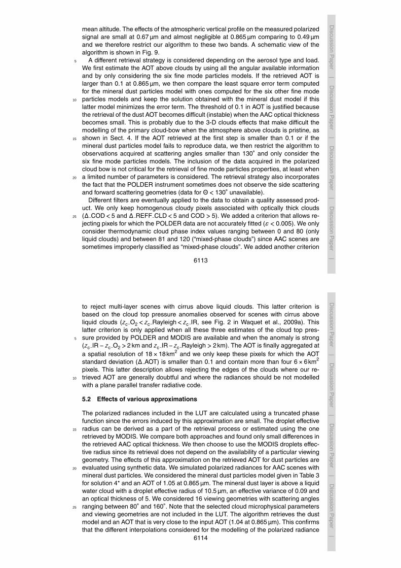
An example of aggregated data is shown in Fig. 6. Two different “branches of scat-tering angle” are usually observed by POLDER when an area of 200×200km2 is con-sidered (e.g. 97◦ <Θ < 177◦ and 157◦ <Θ < 177◦ in Fig. 6a). In the retrieval algorithm,we consider only one “branch of scattering angle” for sake of simplicity. We select thebranch associated with the widest range of scattering angles (e.g. 97◦ <Θ < 177◦ in5

Fig. 6a). Figs. 6a and 6b show that this procedure allows to obtain rather smooth meanpolarized radiances associated with a consistent mean viewing geometry.

3.3.2 Errors’ measurements

The error’s measurements are taken from Fougnie et al. (2007) and are used to fillout the total error covariance matrix. We consider a relative error of calibration of 2 %10

in the three polarized spectral bands. The polarization measurements are acquired byPOLDER using a sequential rotation of polarizers oriented at 0, 60 and −60◦. One ofthe measurements triplets at 0.67 µm was shown to be imperfect by construction, whichtends to increase the noise in the polarized data acquired at this wavelength (see forinstance Fig. 4a). The noise associated with the polarized radiances for cloudy scenes15

is estimated to be 2.5×10−3 at 0.49 µm and 0.865 µm and 5×10−3 at 0.67 µm. Weassume that the different sources of errors are independent and the total covariancematrix is given by the sum of the different error covariance matrices.

3.4 Particles models and a priori information

A combination of two lognormal size distribution functions is assumed for the aerosols.20

A geometric mean radius and a standard deviation are used to describe each lognor-mal function (rg and σ), where rg is the geometric mean radius. The other retrieved

parameters are the column number density of particles (N, in µm−2), for both modes,and the complex refractive index (mr −mi i ) that is assumed to be spectrally invariantand the same in both modes. The effective radius, reff, is related to the lognormal size25

distribution parameters using the formula given in the Appendix A2.

6101

Discussion

Paper

|D

iscussionP

aper|

Discussion

Paper

|D

iscussionP

aper|

For non-spherical particles, we consider spheroid models with various aspect ra-tios to compute the optical properties of the aerosols (Mishchenko and Travis, 1994;Dubovik et al., 2006). We consider a mixture of spherical and non-spherical particles.The ratio of spherical particles over the total number of particles (SF) is included in theretrieval process for AAC scenes with mineral dust particles. The aspect ratios distri-5

bution for the non-spherical particles model is the one derived by Dubovik et al. (2006)from the analysis of the scattering matrix of mineral dust samples (Volten et al., 2001).

The cloud droplets size distribution is assumed to follow a gamma standard law, de-scribed by two parameters, the cloud droplets effective radius, reff cld, and the clouddroplets effective variance, veff cld, as defined in Hansen and Travis (1974). The real re-10

fractive index for cloud droplets, mr cld, is retrieved in each spectral band. The imaginaryrefractive index for cloud droplets is less than 5×10−7 for the POLDER wavelengths(Hale et al., 1973) and it is therefore neglected in the calculations (held constant to 0).Angular polarization measurements are highly sensitive to the real refractive index oflarge spherical particles due to the presence of bows. We make clear that the droplets15

real refractive index is primarily included in the retrieval process to ensure an accuratemodelling of the cloud bows (angular locations and magnitudes). The droplet effectivevariance is also included in the algorithm, since this parameter strongly impacts themagnitude of surnumerary cloud bows. The cloud droplets are modelled as spheresand their optical properties are therefore calculated using the Mie theory.20

In Table 1, we provide the values of the a priori aerosol and cloud parameters (“start-ing point for X”) and the associated uncertainties (Ca). The subscripts f and c respec-tively denote parameters that describe the fine mode and coarse mode aerosols. Thenumber of retrieved parameters included in the OEM can be modified and the a prioriinformation as well. If so, we provide the corresponding information in text.25

6102

Discussion

Paper

|D

iscussionP

aper|

Discussion

Paper

|D

iscussionP

aper|

3.5 Forward model

3.5.1 Transfer radiative code and particles vertical distribution

The polarized radiances are computed using the Successive Order of Scattering code(SOS) that accounts for the effects of multiple scattering under the assumption of theplane parallel atmosphere (Lenoble et al., 2007). The SOS code provides the usual5

three first Stokes parameters and allows including various atmospheric componentsthat are separately described for the optical properties and the vertical profile. Thevertical profile for the molecules is defined using a decreasing exponential law witha scale height of 8 km. The molecular optical thickness and the effects of molecularanisotropy are computed using the formulae given in Hansen and Travis (1974). The10

vertical profile of the aerosol layer is described using a Gaussian distribution function,defined by a standard deviation (0.75) and a mean altitude value, z mean. The clouddroplets particles are assumed well mixed with the molecules between the surface andthe cloud top height. The cloud base height is therefore located at 0 km. The cloud opti-cal thickness is held constant to 5, which ensures that the polarized radiance reflected15

by the cloud layer is saturated. The mean altitude of the aerosol layer and the cloudtop height are adjusted using the lidar data. When those are not available, we use the“apparent O2 cloud pressure” to estimate the cloud top height and assume a meanaltitude z mean of 3.5 km for the AAC height. Then, we apply an empirical correctionon zc O2, defined on the basis of our observations, which accounts for the fact that the20

“apparent O2 cloud pressure” underestimates the cloud top height given by CALIOP.For instance, we used a correction of about 40 % for AAC scenes with mineral dustparticles on the basis of the observations performed on the 4 August 2008 (see Fig. 3bbetween latitudes 19◦ and 23◦).

6103

Discussion

Paper

|D

iscussionP

aper|

Discussion

Paper

|D

iscussionP

aper|

3.5.2 Effects of phase function truncature

The SOS code requires a Legendre polynomial expansion of the phase matrix. The for-ward peak of the phase function (i.e. the P11 element of the phase matrix) is generallysharp for large particles such as cloud particles, which requires to increase the numberof terms in the expansion of the phase matrix. A truncation procedure of the forward5

scattering peak is implemented in the SOS code (Potter, 1970; Nakajima and Tanaka,1998). This procedure allows a faster modelling of the radiances. We however notedthat this procedure introduces small errors in the modelling of the upwelling polarizedradiance under specific circumstances that are encountered in this paper. Errors ap-pear when large spherical particles are considered and when the polarized radiance10

is saturated (optical thickness > 3). Significant errors appear in the primary cloud bowregion. The magnitude of the primary cloud-bow is overestimated by 7.5 % when theprocedure of truncation is invoked. Calculations performed for a truncation applied toscattering angles between 0◦ and 16◦, for a droplet effective radius of 10 µm, a dropleteffective variance of 0.06, cloud optical thickness of 5 and a sun zenith angle of 37◦.15

The reasons for this issue are not fully understood and the solving of this technicalproblem will be attempted in a future effort. In the retrieval algorithm, we use an exact1-D modelling (no truncation) at the end of each step in the iteration to compare the ob-servations to the simulations whereas the intermediate calculations (i.e. the Jacobianmatrix elements) are performed using the approximation of truncature.20

3.5.3 3-D cloud effects

It is well known that the homogeneous 1-D cloud assumption leads to errors in theretrieved cloud parameters from total visible radiance (Marshak and Davis, 2005). Cor-net et al. (2009) show for a cirrus cloud with a Monte-Carlo radiative transfer code thatbiases exist also on polarized radiance. To assess the errors in our 1-D transfer radia-25

tive model, we compute 3-D and 1-D polarized radiance of a stratocumulus cloud witha mean optical thickness of 10 and an uniform effective radius of 10 µm and an effective

6104

Discussion

Paper

|D

iscussionP

aper|

Discussion

Paper

|D

iscussionP

aper|

variance of 0.02. The heterogeneity parameter is 7 for the optical thickness (standarddeviation associated with the mean optical thickness). The initial resolution of the ra-diative transfer simulation is 80×80m2. The radiances are then spatially averaged at10×10km2 to simulate the observation of a sensor like POLDER. The differences be-tween the 1-D and 3-D polarized reflectances in function of the scattering angle are5

presented in Fig. 7 for the three wavelengths used in the algorithm and for different sunangles. For most of the scattering angles, and for the case considered here, which doesnot include microphysical heterogeneity, the differences between the two polarized re-flectances are small and inside the statistical error of the Monte-Carlo simulations (notplotted). Exceptions appears however in the forward direction for large sun angle and10

the cloud bow regions near 140◦. Considering our algorithm, the differences, whichmay impact the most our retrieval, are those in the cloud-bow direction. The 1-D sim-ulations systematically overestimate the ones that account for the 3-D cloud effects byabout 5–8 %, depending on wavelength and geometry (θs, ϕ). Because for computingtime reasons, it is pratically impossible to account for those 3-D effects in our retrieval15

procedure, we incorporated these errors into the total error covariance matrix (CT).

4 Sensitivity study and discussion

4.1 Biomass burning aerosols

The OEM algorithm is flexible and the number of retrieved parameters can be increasedor decreased as needed. We did several tests with varying numbers of retrieved pa-20

rameters in order to provide a sensitivity study. We first investigate the AAC scene withbiomass burning aerosols, referred as box (1) in Fig. 1a. The solutions obtained forvarious retrieval schemes are reported in Table 2. The quantity ω0 denotes the aerosolsingle scattering albedo. The quantity ε is the mean squared difference error termcalculated between measured and simulated polarized radiances (see Appendix A3).25

This quantity gives a simple measure of the difference between measurements and

6105

Discussion

Paper

|D

iscussionP

aper|

Discussion

Paper

|D

iscussionP

aper|

simulations, assuming a diagonal identity matrix for Cx (no weight) and no a prioriknowledge. Note that the quantity ε is consistent with the definition of the error termconsidered in the less sophisticated retrieval method described in Sect. 5. Solution 1includes the retrieval of the parameters of load and size for the fine particles and the mi-crophysical parameters for the clouds particles. We consider spherical particles, which5

is a reasonable assumption for biomass burning aerosols. The value for the sphericalfraction (SF) (spherical fraction of particles) indicated in Table 1 (0.5±0.5) is thereforemodified and held constant to 1. Solution 2 is the same as solution 1 but includes theretrieval of the properties of the coarse mode (load and size parameters). Solutions 1and 2 both assume a weak absorption. Solution 3 is similar as solution 2 with in addition10

the retrieval of the imaginary part of the complex refractive index (i.e. absorption). So-lution 4 is similar as solution 3 but includes the retrieval of the real part of the refractiveindex. The real and imaginary parts of the complex refractive index are assumed to besimilar for both modes. For solution 5, we made assumptions for the coarse mode par-ticles optical thickness (0.015 at 0.865 µm), the coarse mode particles effective radius15

(reff c = 2.55µm) and for the real refractive index (mr = 1.47). Solution 5 is an attemptto reduce the space of solutions by limiting the number of retrieved parameters. Werecall that the aerosol SSA depends on both particles absorption and size distribution.Then, any errors due to the assumptions made about the aerosol properties (e.g. forthe size or the coarse mode AOT) directly affect the retrieval of the aerosol SSA.20

Solution 1 allows to robustly model the POLDER data (not shown) and confirms thatthe polarized measurements are primarily sensitive to the fine mode scattering AOTand its spectral dependence as well as the cloud microphysical properties. The mea-surements are potentially sensitive to the aerosol Single Scattering albedo (SSA) sincethe polarization observed at side scattering angles is related to the scattering AOT25

whereas the effect of attenuation of the aerosol layer on the polarized light reflectedby the cloud depends on the total (extinction) AOT. The algorithm shows some sensi-tivity to the aerosol SSA. We observed that the effect of the absorption on the polar-ized radiances is rather small but not negligible. Solution 4 includes the most degrees

6106

Discussion

Paper

|D

iscussionP

aper|

Discussion

Paper

|D

iscussionP

aper|

of freedom in terms of retrieved aerosol microphysical parameters and retrieves anaerosol model for which the size distribution is dominated by fine mode particles (α ofabout 2.) associated with rather strong absorption properties (mi of 0.017±0.007). Thestandard deviation for each parameter is small, excepted for the coarse mode particleseffective radius, which tends to indicate that the algorithm is sensitive to most of the5

parameters considered in solution 4. The least square error term ε is minimized for thissolution. We however note that the other solutions (1, 2, 3, and 5) allow to accuratelymodel the POLDER data (e.g. see Fig. 8a for solution 5) and shows rather similar lowε values. The retrieved AOTs at 0.865 µm are rather similar for all these solutions butdifferences appear for the aerosol microphysical parameters. For instance, the contri-10

bution of the coarse mode particles to the total AOT is larger for solution 2 than forsolution 4 whereas the absorption is much smaller for solution 2 than for solution 4.

Solution 5 provides an estimate of the aerosol SSA equal to 0.815 (±0.045) at0.865 µm, which is consistent with biomass burning aerosols in South Africa accordingto AERONET sun-photometers observations (Dubovik et al., 2002). The mean aerosol15

SSA is 0.80±0.004 (at 0.87 µm) and the mean imaginary part of the complex refractiveindex is 0.021±0.004, for biomass burning aerosols observed in the centre of SouthAfrica (Zambia). Our estimate also agrees rather well with the one provided by Leahyet al. (2007), who found an aerosol single scattering albedo of 0.85±0.02 (regionalmean and uncertainty at 0.55 µm), on the basis of an updated analysis of remote and20

in situ measurements performed during the Southern African Regional Science Initia-tive 2000 (SAFARI). We also investigated another day in the same region in August2008 for a scene with a retrieved AOT of 0.21 (±0.01) in biomass burning AAC andfound an aerosol SSA of 0.91 (±0.05) at 0.865 µm with solution 5. It is impossible totell if this variability observed from one case to another is due to a real change in the25

aerosol microphysical properties or due to the issue of multiple solutions in our re-trievals. We note that a previous study suggested a higher value for the aerosol SSA(0.91±0.04 at 0.55 µm) for SAFARI (Haywood et al., 2003b) and that some variability

6107

Discussion

Paper

|D

iscussionP

aper|

Discussion

Paper

|D

iscussionP

aper|

in the degree of absorption of the biomass-burning aerosols is expected during the fireseason in South Africa (Eck et al., 2003).

We reported the results obtained for two other “hyper-pixels” in Table 4 that bothcorrespond to scenes with small AAC optical thickness. We used solution 5 to analyzeboth cases. Case (1) in Table 4 corresponds to an AAC scenes encountered for the5

case study on biomass burning aerosols that is referred as box (2) in Fig. 1a. Case (2)corresponds to the data acquired on the 18 August 2008 for clouds observed in pristineconditions between South Africa and Antarctica. The algorithm retrieves a small valueof AOT for case (1) but still retrieves a size distribution dominated by small particles,which suggests a continental origin. The retrieved AOT is very small (0.022±0.003)10

for case (2) and the type of particles then cannot be identified since the Angstromexponent cannot be accurately retrieved anymore (α = 0.88±1.08). Some difficultiesin the modelling of the polarized radiances can be observed for case (1) for largescattering angles (≈ 180◦) that are not clearly understood (see Fig. 8c). We assumethat it could be the result of the scene spatial heterogeneity. In a general way, we15

note that significant errors in the modelling of the polarized radiances appear in thecloud-bow region when the AAC optical thickness is small (see Fig. 8c and d) that areprobably due to 3-D cloud effects. Nevertheless, these two latter results indicate thatthat the AAC optical thickness progressively decreases as we move away from SouthAfrica and that solution 5 remains robust even when the AOT becomes small.20

4.2 Mineral dust particles

We now investigate the AAC scene with mineral dust particles, referred as box (3) inFig. 2a, which was observed on the 25 July 2008. The solutions obtained for variousretrieval schemes are reported in Table 3. Solution 1* includes the retrieval of the fineand coarse mode particles load and size parameters and assumes a constant complex25

refractive index. Solution 2* includes in addition the retrieval of the imaginary part of thecomplex refractive index whereas solution 4 includes both the retrieval of the real andimaginary parts of the complex refractive index. For solution 4*, we made assumptions

6108

Discussion

Paper

|D

iscussionP

aper|

Discussion

Paper

|D

iscussionP

aper|

for the coarse particles size parameter and for the real refractive index. The fractionof spherical particles (SF) is included in the retrieval scheme for all solutions and it isassumed the same in both modes.

The different solutions (1*, 2*, 3* and 4*) allows robust modelling the POLDER ob-servations (e.g. see Fig. 8b for solution 4*). The algorithm retrieves AOT values larger5

than 1 and a large amount of non-spherical particles. The coarse mode effective radiusretrieved for solutions 1*, 2* and 3* is too large and clearly not realistic for mineral dustparticles. The standard deviation values for the coarse mode effective radius are alsovery large, which means that this parameter cannot be accurately retrieved. Again mul-tiple solutions are possible and some assumptions must be considered. For solution10

4*, the algorithm then retrieves a size distribution dominated by non-spherical coarsemode particles that shows much smaller absorption properties than biomass burningaerosols. Mineral dust particles also absorb the solar light due to the presence of ironoxide in their mineral composition (Derimian et al., 2008a). However, dust remainsless absorbing than biomass burning aerosols, except probably for cases where it is15

mixed with carbonaceous material (Derimian et al., 2008b). Note that we should haveretrieved the spectral dependence for the imaginary part of the complex refractive in-dex since mineral dust particles typically show slightly higher absorption properties forshorter visible wavelengths (0.49 µm) than for larger wavelengths (0.67 and 0.865 µm).We however choose to hold constant this parameter with respect with wavelength to20

limit the number of retrieved parameters. This would have to be revised in case shorterwavelength observations would be incorporated.

We reported in Table 4 the results for the AAC scene with mineral dust particlesobserved on the 4 August 2008. The hyper-pixel is referred as box (4) in Fig. 3a andcorresponds to case (3) in Table 4. We used solution 4* to analyze the data. The25

algorithm again retrieves the typical properties assumed for mineral dust particles. Weobserve that the contribution of the fine mode particles to the total AOT is much smaller(lower value of Angstrom exponent) than for the July case. Such variability in the sizedistribution of mineral dust particles is realistic according to Dubovik et al. (2002).

6109

Discussion

Paper

|D

iscussionP

aper|

Discussion

Paper

|D

iscussionP

aper|

4.3 General comments on the refractive index retrieval

We generally retrieve a real refractive index lower than 1.47, when we include this pa-rameter in the retrieval scheme for biomass burning aerosols but also for mineral dustparticles. Dubovik et al. (2002) indicates an effective radius of about 0.13 µm (com-puted for an optical thickness of 0.9 at 0.44 µm) and real refractive index of 1.51, for5

biomass burning aerosols in the centre of South Africa. Our results indicate a largereffective radius (0.17 µm) and a smaller real refractive index (1.45±0.015, see solution4 in Table 3). The retrieved real part of the refractive index is also very low for mineraldust particles (1.41±0.035). We noted that the decrease in the real refractive index inour retrievals is generally associated with an increase in the fine mode effective radius.10

This result suggests the AAC properties could be altered (an aged effect), which islikely to be possible since aerosols mix with wet air masses when they are transportedover long distance in oceanic regions.

Knobelspiesse et al. (2011) found some difficulties in retrieving the real refractiveindex for AAC scenes with anthropogenic aerosols. They analyzed the off diagonal15

elements of the retrieval error covariance matrix and found large correlations betweenthe errors associated with the retrieved particles real refractive index and size. Wesuggest that the retrieval of these two parameters is linked since they both largely affectthe magnitude of the polarized phase function and affect it in an opposite way. Roughly,the P12 elements increase with the particles size increasing and the real refractive20

index decreasing. Polarized radiances measured over cloud-free ocean scenes showhigh sensitivity to the particles real refractive index for scattering angles larger than130◦ (e.g. see Figs. 6 and 12 in Deuze et al., 2000). We assume that some informationabout the aerosol microphysics is lost for AAC scenes by comparison with clear-skyocean scenes, probably because the contribution of the cloud layer dominates the25

signal for scattering angles larger than 130◦.We also noted that the inclusion of the errors due to the 3-D cloud effects in the total

error retrieval covariance matrix leads to the retrieval of weaker absorption properties

6110

Discussion

Paper

|D

iscussionP

aper|

Discussion

Paper

|D

iscussionP

aper|

(smaller values for mi ) and therefore higher values of aerosol SSA. The retrieved valuesfor the imaginary part of the complex refractive index are generally too times higherwhen the 3-D cloud effects are not accounted for.

4.4 Cloud droplets

The retrieved real refractive index values are in good agreement with what we expect for5

cloud droplets made of pure water (Hale et al., 1973). Our algorithm retrieves dropletseffective radii varying between 8 and 12 µm with no peculiar geographical tendency.The retrieved droplets size distribution is much narrower (small values of effective vari-ance) for the clouds observed southerneastern of the South Africa than for the cloudsobserved over the two other oceanic tropical regions located closer to Africa. This is10

good agreement with the results of Breon and Doutriaux-Boucher (2005), who foundthat the droplets effective variance is generally much smaller for the clouds observedin subtropical and high-latitude oceans, than for continental regions and other oceanicregions. The reasons for this tendency cannot be currently established with confidence.We recall that the droplets effective variance was not much studied from space and that15

this parameter depends on the dynamical evolution of clouds (Politovich, 1993) and onthe origin of the air mass (continental or maritime) (Martin et al., 2004).

Finally, we also compared the droplet effective radii retrieved with POLDER withthose retrieved by MODIS. Table 5 show some comparisons performed for variousscenes with aerosols above clouds and for the fields of clouds observed in pristine20

conditions. The droplet effective radius reported for MODIS is a mean value com-puted over the 200km×200km area. Differences are expected between these twoestimates since the polarized measurements are sensitive to droplets located at thetop of the cloud layer whereas the MODIS total radiance measurements are sensitiveto droplets located deeper in the cloud layer (Breon and Doutriaux-Boucher, 2005).25

Another sources of differences are (1) that biases are expected on the MODIS re-trieved droplets effective radius for AAC scenes with absorbing aerosols and (2) thatthe droplets effective variance is held constant in the MODIS algorithm (0.13). Breon

6111

Discussion

Paper

|D

iscussionP

aper|

Discussion

Paper

|D

iscussionP

aper|

and Doutriaux-Boucher (2005) found a systematic MODIS high bias of 2 µm in oceanicregions for droplets effective radii larger than 7 µm. The results obtained for the cloudsobserved in pristine conditions show a rather similar bias. The departures that we ob-served for AAC scenes are smaller than 2 µm, probably because the droplets effectiveradii retrieved by MODIS are underestimated due to the presence of absorbing AAC5

(Haywood et al., 2004).

5 Operational algorithm: the “single-pixel method”

5.1 Description

We use a look-Up-Table (L.U.T) approach to derive the aerosol properties above cloudsusing the observations acquired by POLDER at a fine spatial resolution. With respect10

with the so-called “hyper-pixel” method described in Sect. 3, we reduce the numberof retrieved parameters to the AOT, the Angstrom exponent and the cloud droplets ef-fective radius. The effects of the droplets effective radius and AOT are illustrated inFig. 5. We calculate the polarized radiances using the SOS code for different com-binations of aerosol and cloud particles models. We consider six fine mode aerosols15

models (rgf=0.06, 0.08, 0.1, 0.12, 0.14, 0.16 µm and σf =0.4) with a constant com-

plex refractive index of 1.47–0.01i , which is a mean value for polluted and biomassburning aerosols. We also included the mineral dust particles model described inTable 3 (solution 4*). The elements of the polarized phase function were shown forsimilar particles models in previous studies (e.g. see Figs. 1 and 2 in Waquet et al.,20

2007). The polarized radiances are calculated for various AOTs and viewing geome-tries and interpolation processes are considered. For clouds particles, we consider25 droplets models with effective radius varying between 5 and 26 µm by step of1 µm, with a constant droplets variance of veff cld = 0.06 and a constant real refractiveindex (mr cld(0.490µm) = 1.338,mr cld(0.670µm) = 1.331 and mr cld(0.865µm) = 1.33).25

We assume a cloud top height of 0.75 km and a value of 3.5 km for the aerosol layer

6112

Discussion

Paper

|D

iscussionP

aper|

Discussion

Paper

|D

iscussionP

aper|

mean altitude. The effects of the atmospheric vertical profile on the measured polarizedsignal are small at 0.67 µm and almost negligible at 0.865 µm comparing to 0.49 µmand we therefore restrict our algorithm to these two bands. A schematic view of thealgorithm is shown in Fig. 9.

A different retrieval strategy is considered depending on the aerosol type and load.5

We first estimate the AOT above clouds by using all the angular available informationand by only considering the six fine mode particles models. If the retrieved AOT islarger than 0.1 at 0.865 µm, we then compare the least square error term computedfor the mineral dust particles model with ones computed for the six other fine modeparticles models and keep the solution obtained with the mineral dust model if this10

latter model minimizes the error term. The threshold of 0.1 in AOT is justified becausethe retrieval of the dust AOT becomes difficult (instable) when the AAC optical thicknessbecomes small. This is probably due to the 3-D clouds effects that make difficult themodelling of the primary cloud-bow when the atmosphere above clouds is pristine, asshown in Sect. 4. If the AOT retrieved at the first step is smaller than 0.1 or if the15

mineral dust particles model fails to reproduce data, we then restrict the algorithm toobservations acquired at scattering angles smaller than 130◦ and only consider thesix fine mode particles models. The inclusion of the data acquired in the polarizedcloud bow is not critical for the retrieval of fine mode particles properties, at least whena limited number of parameters is considered. The retrieval strategy also incorporates20

the fact that the POLDER instrument sometimes does not observe the side scatteringand forward scattering geometries (data for Θ < 130◦ unavailable).

Different filters are eventually applied to the data to obtain a quality assessed prod-uct. We only keep homogenous cloudy pixels associated with optically thick clouds(∆ COD<5 and ∆ REFF CLD<5 and COD > 5). We added a criterion that allows re-25

jecting pixels for which the POLDER data are not accurately fitted (ε < 0.005). We onlyconsider thermodynamic cloud phase index values ranging between 0 and 80 (onlyliquid clouds) and between 81 and 120 (“mixed-phase clouds”) since AAC scenes aresometimes improperly classified as “mixed-phase clouds”. We added another criterion

6113

Discussion

Paper

|D

iscussionP

aper|

Discussion

Paper

|D

iscussionP

aper|

to reject multi-layer scenes with cirrus above liquid clouds. This latter criterion isbased on the cloud top pressure anomalies observed for scenes with cirrus aboveliquid clouds (zc O2 <zc Rayleigh<zc IR, see Fig. 2 in Waquet et al., 2009a). Thislatter criterion is only applied when all these three estimates of the cloud top pres-sure provided by POLDER and MODIS are available and when the anomaly is strong5

(zc IR− zc O2 >2 km and zc IR−zc Rayleigh > 2km). The AOT is finally aggregated ata spatial resolution of 18×18km2 and we only keep these pixels for which the AOTstandard deviation (∆ AOT) is smaller than 0.1 and contain more than four 6×6km2

pixels. This latter description allows rejecting the edges of the clouds where our re-trieved AOT are generally doubtful and where the radiances should be not modelled10

with a plane parallel transfer radiative code.

5.2 Effects of various approximations

The polarized radiances included in the LUT are calculated using a truncated phasefunction since the errors induced by this approximation are small. The droplet effectiveradius can be derived as a part of the retrieval process or estimated using the one15

retrieved by MODIS. We compare both approaches and found only small differences inthe retrieved AAC optical thickness. We then choose to use the MODIS droplets effec-tive radius since its retrieval does not depend on the availability of a particular viewinggeometry. The effects of this approximation on the retrieved AOT for dust particles areevaluated using synthetic data. We simulated polarized radiances for AAC scenes with20

mineral dust particles. We considered the mineral dust particles model given in Table 3for solution 4* and an AOT of 1.05 at 0.865 µm. The mineral dust layer is above a liquidwater cloud with a droplet effective radius of 10.5 µm, an effective variance of 0.09 andan optical thickness of 5. We considered 16 viewing geometries with scattering anglesranging between 80◦ and 160◦. Note that the selected cloud microphysical parameters25

and viewing geometries are not included in the LUT. The algorithm retrieves the dustmodel and an AOT that is very close to the input AOT (1.04 at 0.865 µm). This confirmsthat the different interpolations considered for the modelling of the polarized radiance

6114

Discussion

Paper

|D

iscussionP

aper|

Discussion

Paper

|D

iscussionP

aper|

only weakly affect the retrieval of the AOT. We perturbed the retrieval by increasing anddecreasing the droplets effective radius, respectively by 2 µm and found a maximal er-ror of 0.03 in the AOT. We decreased by 14 % the magnitude of the synthetic polarizedradiances in the cloud-bow directions to evaluate the impacts on the AOT due to theuncertainties in modelling the primary cloud-bow magnitude (due to 3-D cloud effects5

and truncation effects). We found that the algorithm then overestimates the true AOTby 12.5 %. The error reaches 14 % if we also perturb the cloud droplet effective radiusby 2 µm at the same time. We also note that the errors slightly increase when a smallvalue of cloud droplet variance is considered in the input simulation (e.g. 0.03 insteadof 0.09). Note that these different sources of errors only weakly affect the retrieval of10

fine mode particles properties, for which we only consider data acquired for scatteringangles smaller than 130◦. Note also that this analysis does not account for potentialerrors due to the assumptions made for the aerosol microphysical properties.

5.3 First results

5.3.1 Case studies15

The spatial variability of the AOT of the dust plume transported above clouds on the25 August 2008 is shown in Fig. 10a, together with the AOT retrieved over cloud-freeocean. This is a combination of AOT retrieved with the operational algorithm for cloud-free scenes (Herman et al., 2005) and with method previously described for cloudyscenes. The AOT map shows that the dust plume is blowing east over the ocean and20

then southeast above low-level clouds. The AAC algorithm retrieves the dust modelincluded in the LUT and the retrieved Angstrom exponent is therefore about 0.4. Fig-ure 10a shows a good qualitative spatial agreement between the AOTs retrieved overcloudy and cloud-free pixels. We however note that the AAC optical thicknesses aresystematically smaller than the ones retrieved over clear-sky ocean pixels. For in-25

stance, the maximal AOT retrieved above clouds and cloud-free ocean are, respectivelyequal to 1.5 and 1.7. Such a difference is not surprising since the AAC optical thickness

6115

Discussion

Paper

|D

iscussionP

aper|

Discussion

Paper

|D

iscussionP

aper|

does not include the aerosols located in the lower atmosphere layer that were detectedover cloud-free scenes by CALIOP. The results obtained for the mineral dust particlesobserved on the 4 August 2008 are reported in Fig. 10b. The same observations canbe made for this second case study. The fact that the algorithm does not retrieved AOTover clouds that are larger than the total column AOT is also a positive sign of the5

retrieval consistency.For the case study on the biomass burning aerosols, we compare the AAC optical

thickness with the fine mode AOT retrieved by POLDER over cloud-free pixels. We as-sume that most of the fine mode particles are located in the elevated biomass burningaerosols layer. Therefore, the fine mode AOT retrieved above cloud-free pixels with the10

ocean algorithm and the AAC optical thickness retrieved with anthropogenic particlesmodels should be rather comparable. Figure 11b shows a general good qualitative spa-tial agreement between the AOTs retrieved over both type of scenes. The largest AACoptical thicknesses (> 0.3) are retrieved over the Gulf of Guinea and are associatedwith small particles (α of ≈ 2.25). In this region, the AAC optical thicknesses are higher15

than the AOTs retrieved for ocean scenes. In this region, the spatial variability of thefine mode AOT retrieved over clear-sky ocean pixels is sometimes questionable. Forinstance, the fine mode AOT abruptly changes from about 0.16 to 0.24 (from blue toyellow in the AOT map shown in Fig. 11a) around the point of coordinates longitude4◦ and latitude −9◦. The change in the fine mode AOT is associated with a change20

on the coarse mode microphysical properties (the fraction of non-spherical particleschanged). Biomass burning aerosols are very likely to be strong absorbing particles.We think that the assumption of non-absorbing particles made in the ocean algorithmmight lead this method to slightly overestimate the coarse mode AOT and then to con-sequently underestimate the scattering fine mode AOT. This hypothesis is supported25

by the results of the sensitivity analysis presented in this work showed that the as-sumption of a weak absorption generally leads to the retrieval of a larger coarse modeAOT (see solutions 2 and 4 in Table 2).

6116

Discussion

Paper

|D

iscussionP

aper|

Discussion

Paper

|D

iscussionP

aper|

5.3.2 Mean results

We reported the AOT retrieved at 0.865 µm above clouds with the previous method forfour different regions of the Earth in Fig. 12. We report average values computed overa period of three months. The investigated time period is from 1 June to 31 August2008. We considered four large grid square areas that mainly include ocean cloudy5

scenes. Two areas are centered on the regions previously introduced in Sect. 3. Weselected two other regions respectively located in the northeastern and southeasternparts of the Pacific Ocean where low-level cloud decks are typically present.

The largest AOTs are retrieved over the tropical North East Atlantic region closeto Sahara. The algorithm detects mineral dust particles. The AOT varies between 0.310

and 0.8 and reaches maximal values near the African coasts and the mean Angstromexponent is about 0.4. The scale color was not stretched to make more visible theaerosols structures observed near California. Other average large AOT values (> 0.2)are retrieved for the tropical southeast Atlantic region near the regions of vegetationfires in South Africa. Figure 13 shows a zoom for the mean Angstrom exponent re-15

trieved above clouds for this region. The algorithm retrieves small particles models. Weobserve a decrease in the Angstrom exponent as we progressively move away fromSouth Africa. The mean Angstrom exponent progressively decreases from 2.4 to 1.7,from the east to the west, which corresponds to an increase of 0.06 µm for the effectiveradius in our aerosol model database.20

Low-level clouds typically cover the region of the Pacific Ocean that boards the SouthAmerica coasts along Peru and Chile. According to our results, this region does notshow significant occurrence of aerosols above clouds. The presence of biomass burn-ing aerosols is expected in South America in August but the Andes Mountain certainlyprevents anthropogenic aerosols to be transported over this part of the Pacific Ocean,25

at least for the considered time period. A significant aerosol above cloud signal (AOTof about 0.1) is observed over the Pacific Ocean near the Californian coasts. Severalvegetation fires occurred in California during the summer 2008 due to an exceptional

6117

Discussion

Paper

|D

iscussionP

aper|

Discussion

Paper

|D

iscussionP

aper|

dry spring and the transport of biomass burning aerosols above clouds is very likely,although regional circulation does not usually transport aerosols westwards. The algo-rithm retrieves a mean small Angstrom exponent (≈ 2.1), which confirms the presenceof fine mode particles.

6 Conclusions5

This study confirms that passive sensors with angular, spectral and polarized capa-bilities have a strong potential for retrieving the Aerosols Above Clouds (AAC) opticaland microphysical properties. We developed two different algorithms to analyze thePOLDER data for AAC scenes. The first one, the so-called the “hyper-pixel” method,allows a simultaneous retrieval of the aerosol and cloud properties and uses POLDER10

data aggregated at a coarse resolution. The method retrieves the mean properties ofthe observed particles under the assumption of spatial homogeneity. The sensitivityanalysis presented in this work showed that polarization measurements provided byPOLDER do not contain enough information to fully constrains all the AAC properties.For aerosols, the method is primarily sensitive to the aerosol optical thickness, size dis-15

tribution, shape and real refractive index. The retrieval of the complex refractive indexhowever remains difficult. Our results suggest that the size and the real refractive indexof fine mode aerosols could be respectively larger and smaller when the particles areobserved above clouds, in oceanic regions, than when these particles are observedover land near the sources. We make clear that this method cannot be used to retrieve20

the aerosol SSA since the method failed to accurately separate the absorption opticalthickness and the coarse mode optical thickness for AAC scenes with biomass burningaerosols.

The aerosols layer attenuates the magnitudes of the primary and surnumerary cloudbows generated by the underlying liquid cloud layer. This effect must be corrected25

(or included in the retrieval process) if an accurate estimate of the cloud dropletsmicrophysical properties has to be achieved for AAC retrievals from polarization

6118

Discussion

Paper

|D

iscussionP

aper|

Discussion

Paper

|D

iscussionP

aper|

measurements. Our results confirm that the droplets size distribution is narrow in highlatitude ocean regions and that the droplets effective radius retrieved from polarizationmeasurements is generally slightly smaller than the one retrieved by passive sensorsthat uses total radiance measurements, such as the MODIS instrument (departuressmaller than 2 µm). We found that the magnitude of the primary cloud bow cannot be5

accurately estimated with a plane parallel transfer radiative code. Using a 3-D radiativetransfer code, we shown that the values are reduced in the cloud-bow. The errors forthe modelling of the polarized radiances vary between 5 and 8 %, for the case done,depending on wavelength and viewing geometry. The use of this method for a globaltreatment could certainly benefit for both the aerosol and cloud studies. This method is10

however currently too time consuming and requires an aggregation of the data that isnot always possible. We plan to use this method for further case studies analysis.

A less sophisticated algorithm was developed to retrieve the AOT and the Angstromexponent for AAC scenes at a fine spatial resolution in a more operational processing.With respect with the algorithm described in Waquet et al. (2009a), we improved the15

accuracy of the modelling, included a realistic mode for mineral dust particles anddeveloped a retrieval strategy that takes advantage of the measurements acquiredin the cloud-bow direction. The method is however limited to observations acquiredfor optically thick clouds (optical thickness > 5) and only considers a finite numberof aerosol models. An interesting result of this study is that polarized measurements20

acquired in the cloud-bow can be used to retrieve the optical thickness of the mineraldust particles residing above liquid clouds. These large non-spherical particles do notmuch polarize light but strongly attenuate the polarized cloud bow generated by thebeneath liquid cloud layer. The spectral attenuation can be used to qualitatively identifythe nature of the particles (coarse or fine mode particles) whereas the magnitude of25

the attenuation is related to the optical thickness of the aerosol layer. We compared theAOTs retrieved above clouds with ones retrieved closely over clear-sky ocean pixels.We found maximal differences of 0.2 in AOT at 0.865 µm that can be explained either bythe assumptions used for the microphysical properties of the aerosols, that are different

6119

Discussion

Paper

|D

iscussionP

aper|

Discussion

Paper

|D

iscussionP

aper|

in the two algorithms, or because the algorithm developed for cloud-free ocean scenesmeasures the aerosol load integrated over the entire atmospheric column whereas theAAC algorithm only retrieves the AOT of the particles residing above the cloud top.

More efforts are needed to better characterize the aerosols above clouds properties.The AOT retrieved with the lidar CALIOP could be considered in future efforts to check5

the coherence of our retrievals made over clouds or to better constrain the retrievalof the aerosol microphysics using innovative synergetic approaches. Other POLDERdata could be also potentially included in the method, such as the total radiance mea-surements. We however point out that the present algorithm, solely based on the useof polarization measurements, has the high advantage, with respect with other passive10

methods, of being independent on the albedo of the cloud layer.When a high loading of strong absorbing aerosols is present above clouds, a rather

strong positive radiative forcing is expected as well as significant biases on the re-trieved cloud properties. The first results obtained with POLDER indicate large meanAOTs above clouds for oceanic regions near the coasts of South Africa and California15

that correspond to biomass burning aerosols whereas even larger mean AOTs aboveclouds are retrieved near the coasts of Senegal (for June–August 2008). More inves-tigations are therefore needed to better describe the spatial and temporal variabilityof the AAC properties. Our next step is to analyze the complete archive of POLDERdata for AAC scenes. This would provide a first global estimate of the properties of the20

aerosols suspended above clouds and so to first estimate the much uncertain aerosoldirect forcing over cloudy skies.

Appendix A

The retrieval error covariance matrix for the optical thickness τ.

Cτ = KτCXKTτ (A1)25

6120

Discussion

Paper

|D

iscussionP

aper|

Discussion

Paper

|D

iscussionP

aper|

where Kτ is the Jacobian matrix for τ. The same formula stands for the aerosol singlescattering albedo (ω0) and effective radius (reff).

The effective radius, reff, for log normal size distribution is defined as:

reff = rg exp(

52σ2

)(A2)

Mean squared error term ε calculated between the measured and calculated polarized5

radiances:

ε =

√√√√√ 1NΘNλ

NΘ∑i=1

Nλ∑j=1

[Lmesi j (Θ)−Lcalc

i j (Θ)]2

(A3)

where Nλ and NΘ are, respectively the number of selected viewing directions and thenumber of channels.

References10

Ackerman, A. S., Toon, O. B., Stevens, D. E., Heymsfeld, A. J., Ramanathan V., andWelton. E. J.: Reduction of tropical cloudiness by soot, Science, 288, 1042–1047,doi:10.1126/science.288.5468.1042, 2000.

Ackermann, J.: The extinction-to-backscatter ratio of tropospheric aerosol: a numerical study, J.Atmos. Ocean. Tech., 15, 1043–1050, 1998.15

Breon, F.-M. and Doutriaux-Boucher, M.: A comparison of cloud droplet radii measured fromspace, IEEE T. Geosci. Remote, 43, 1796–1805, 2005.

Breon, F.-M. and Goloub, P.: Cloud droplet effective radius from spaceborne polarization mea-surements, Geophys. Res. Lett., 25, 1879–1882, 1998.

Breon, F.-M., Tanre, D., and Generoso, S.: Aerosol effect on cloud droplet size monitored from20

satellite, Science, 295, 834–838, 2002.

6121

Discussion

Paper

|D

iscussionP

aper|

Discussion

Paper

|D

iscussionP

aper|

Cattrall, C., Reagan, J., Thome, J. K., and Dubovik, O.: Variability of aerosol and spectral lidarand backscatter and extinction ratios of key aerosol types derived from selected aerosolrobotic network locations, J. Geophys. Res., 110, D10S11, doi:10.1029/2004JD005124,2005.

Chand, D., Wood, R., Anderson, T. L., Satheesh, S. K., and Charlson, R. J.: Satellite-derived5

direct radiative effect of aerosols dependent on cloud cover, Nat. Geosci., 2, 181–184, 2009.Chen, B., Huang, J., Minnis, P., Hu, Y., Yi, Y., Liu, Z., Zhang, D., and Wang, X.: Detection of dust

aerosol by combining CALIPSO active lidar and passive IIR measurements, Atmos. Chem.Phys., 10, 4241–4251, doi:10.5194/acp-10-4241-2010, 2010.

Coddington, O. M., Pilewskie, P., Redemann, J., Platnick, S., Russell, P. B., Schmidt, K. S.,10

Gore, W. J., Livingston, J., Wind G., and Vukicevic, T.: Examining the impact of overlyingaerosols on the retrieval of cloud optical properties from passive remote sensing, J. Geophys.Res., 115, D10211, doi:10.1029/2009JD012829, 2010.

Cornet, C., Labonnote L. C., and Szczap, F.: Three-dimensional Polarized Monte-CarloAtmospheric Radiative Transfer Model (3DMCPOL): 3-D effects on polarized visible15

reflectances of a cirrus cloud, J. Quant. Spectrosc. Rad. Transfer, 111, 174–186,doi:10.1016/j.jqsrt.2009.06.013, 2010.

De Graaf, M., Stammes P., and Aben, E. A. A.: Analysis of reflectance spectra of UV-absorbing aerosol scenes measured by SCIAMACHY, J. Geophys. Res., 112, D02206,doi:10.1029/2006JD007249, 2007.20

Derimian, Y., Karnieli, A., Kaufman, Y. J., Andreae, M. O., Andreae, T. W., Dubovik, O., Maen-haut, W., and Koren, I.: The role of iron and black carbon in aerosol light absorption, Atmos.Chem. Phys., 8, 3623–3637, doi:10.5194/acp-8-3623-2008, 2008a.

Derimian, Y., Leon, J.-F., Dubovik, O., Chiapello, I., Tanre, D., Sinyuk, A., Auriol, F., Podvin, T.,Brogniez, G., and Holben, B. N.: Radiative properties of aerosol mixture observed during25

the dry season 2006 over M’Bour, Senegal (African monsoon multidisciplinary analysis cam-paign), J. Geophys. Res., 113, D00C09, doi:10.1029/2008JD009904, 2008b.

Deuze J.-L., Goloub, P., Herman, M., Marchand, A., Perry, G., Tanre, D., and Susana, S.: Esti-mate of the aerosols properties over the ocean with POLDER, J. Geophys Res, 105, 15329–15346, 2000.30

Dubovik, O., Holben, B. N., Eck, F. T., Smirnov, A., Kaufman, J. Y., King, D. M., Tanre, D., andSlutsker, I.: Variability of absorption and optical properties of key aerosol types observed inworldwide locations, J. Atmos. Sci., 59, 590–608, 2002.

6122

Discussion

Paper

|D

iscussionP

aper|

Discussion

Paper

|D

iscussionP

aper|

Dubovik, O., Sinyuk, A., Lapyonok, T., Holben, B. N., Mishchenko, M., Yang, P., Eck, T. F.,Volten, H., Munoz, O., Veihelmann, B., van der Zande, W. J., Leon, J.-F., Sorokin, M., andSlutsker, I.: Application of spheroid models to account for aerosol particle nonsphericity inremote sensing of desert dust, J. Geophys. Res., 111, D11208, doi:10.1029/2005JD006619,2006.5

Eck, T. F., Holben, B. N., Ward, D. E., Mukelabai, M. M., Dubovik, O., Smirnov, A., Schafer, J. S.,Hsu, N. C., Piketh, S. J., Queface, A., Le Roux, J., Swap, R. J., and Slutsker, I.: Variability ofbiomass burning aerosol optical characteristics in southern Africa during the SAFARI 2000dry season campaign and a comparison of single scattering albedo estimates from radiomet-ric measurements, J. Geophys. Res., 108, 8477–8493, doi:10.1029/2002JD002321, 2003.10

Ferlay, N., Thieuleux, F., Cornet, C., Davis, A. B., Dubuisson, P., Ducos, F., Parol, F., Riedi,J., and Vanbauce, C.: Toward new inferences about cloud structures from multidirec-tional measurements in the oxygen A band: Middle-of-cloud pressure and cloud geo-metrical thickness from POLDER3/PARASOL, J. Appl. Meteorol. Clim, 49, 2492–2507,doi:10.1175/2010JAMC2550.1, 2010.15

Forster, P., Ramaswamy, V., Artaxo, P., Berntsen, T., Betts, R., Fahey, D. W., Haywood, J., Lean,J., Lowe, D. C., Myhre, G., Nganga, J., Prinn, R., Raga, G., Schulz, M., and Van Dorland, R.:Changes in Atmospheric Constituents and in Radiative Forcing, in Climate Change 2007:The Physical Science Basis. Contribution of Working Group I to the Fourth AssessmentReport of the Intergovernmental Panel on Climate Change, edited by: Solomon, S., Qin, D.,20

Manning, M., Chen, Z., Marquis, M., Averyt, K. B., Tignor, M., and Miller, H. L., CambridgeUniversity Press, Cambridge, UK and New York, NY, USA, 129–234, 2007.

Fougnie, B., Bracco, G., Lafrance, B., Ruffel, C., Hagolle, O., and Tinel, C.: PARASOL in-flightcalibration and performance, Appl. Opt., 46, 5435–5451, 2007.

Goloub, P., Deuze J.-L., Herman, M., and Fouquart, Y.: Analysis of the POLDER polarization25

measurements performed over cloud covers, IEEE T. Geosci. Remote, 32, 78–88, 1994.Hale, G. M. and Querry, M. R.: Optical constants of water in the 200-nm to 200-µm wavelength

region, Appl. Opt., 12, 555–563, 1973.Hansen, J. E. and Travis, L. D.: Light scattering in planetary atmospheres, Space Sci. Rev., 16,

527–610, doi:10.1007/BF00168069, 1974.30

Hasekamp, O. P.: Capability of multi-viewing-angle photo-polarimetric measurements for thesimultaneous retrieval of aerosol and cloud properties, Atmos. Meas. Tech., 3, 839–851,doi:10.5194/amt-3-839-2010, 2010.

6123

Discussion

Paper

|D

iscussionP

aper|

Discussion

Paper

|D

iscussionP

aper|

Haywood, J. M. and Boucher, O.: Estimates of the direct and indirect radiative forcing due totropospheric aerosols: a review., Revs. Geophys., 38, 513–543, 2000.

Haywood, J. M., Osborne, S. R., Francis, P., Glew, M., Highwood, E., Formenti, P., and An-dreae, M.: Radiative properties and direct radiative effect of Saharan dust measured bythe C-130 aircraft during SHADE: 1. Solar spectrum, J. Geophys. Res., 108, 8577–8592,5

doi:10.1029/2002JD002687, 2003a.Haywood, J. M., Osborne, S. R., Francis, P. N., Keil, A., Formenti, P., Andreae, O. M., and Kaye,

P. H.: The mean physical and optical properties of regional haze dominated by biomassburning aerosol measured from the C-130 aircraft during SAFARI 2000, J. Geophys. Res.,108, 8473–8486, 2003b.10

Haywood, J. M., Osborne, S. R., and Abel, S. J.: The effect of overlying absorbing aerosol layerson remote sensing retrievals of cloud effective radius and cloud optical depth, Q. J. Roy.Meteorol. Soc., 130, 779–800, 2004.

Herman, M., Deuze, J.-L., Marchand, A., Roger, B., and Lallart, P.: Aerosol remote sensing fromPOLDER/ADEOS over the ocean: improved retrieval using a nonspherical particle model, J.15

Geophys. Res., 110, D10S02, doi:10.1029/2004JD004798, 2005.Hsu, N. C., Herman, J. R., and Chen, S.-C.: Radiative impacts from biomass burning in the

presence of clouds during boreal spring in southeast Asia, Geophys. Res. Lett., 30, 1224–1227, doi:10.1029/2002GL016485, 2003.

Hu, Y., Vaughan, M., Liu, Z., Powell, K., and Rodier., S.: Retrieving optical depths and lidar20

ratios for transparent layers above opaque water clouds from calipso lidar measurements,IEEE Geosci. Remote Sens. Lett., 4, 523–526, 2007.

Johnson, B. T., Shine, K. P., and Forster, P. M.: The semi-direct aerosol effect: impact ofabsorbing aerosols on marine stratocumulus, Q. J. R. Meteorol. Soc., 130, 1407–1422,doi:10.1256/qj.03.61, 2004.25

Kaufman, Y., Tanre, D., and Boucher, O.: A satellite view of aerosols in the climate system,Nature, 419, 215–223, 2002.

Kalashnikova, O. V., Kahn, R., Sokolik, I. N., and Li, W.-H.: Ability of multiangle remote sensingobservations to identify and distinguish mineral dust types: optical models and retrievals ofoptically thick plumes, J. Geophys. Res., 110, D18S14, doi:10.1029/2004JD004550, 2005.30

Keil, A. and Haywood, J. M.: Solar radiative forcing by biomass burning aerosol particles duringSAFARI 2000: A case study based on measured aerosol and cloud properties, J. Geophys.Res., 108, 8467–8476, 2003.

6124

Discussion

Paper

|D

iscussionP

aper|

Discussion

Paper

|D

iscussionP

aper|

Knobelspiesse, K., Cairns, B., Redemann, J., Bergstrom, R. W., and Stohl, A.: Simultaneousretrieval of aerosol and cloud properties during the MILAGRO field campaign, Atmos. Chem.Phys., 11, 6245–6263, doi:10.5194/acp-11-6245-2011, 2011.

Leahy, L. V., Anderson, T. L., Eck, T. F., and Bergstrom, R. W.: A synthesis of single scatteringalbedo of biomass burning aerosol over Southern Africa during SAFARI 2000, Geophys.5

Res. Lett., 34, L12814, 2007.Lenoble, J., Herman, M., Deuze, J. L., Lafrance, B., Santer, R., and Tanre, D.: A successive

order of scattering code for solving the vector equation of transfer in the earths atmospherewith aerosols Journal of Quantitative Spectroscopy and Radiative Transfer, 107, 479–507,doi:10.1016/j.jqsrt.2007.03.010, 2007.10

Martin, G. M., Johnson, D. W., and Spice, A.: The measurement and parameterization of effec-tive radius of droplets in warm stratocumulus clouds, J. Atmos. Sci., 51, 1823–1842, 1994.

Marshak, A. and Davis, A. B.: 3-D Radiative Transfer in Cloudy Atmospheres, Springer, NewYork, p. 686, 2005.

Menzel, W. P., Frey, R. A., Baum, B. A., and Zhang, H.: Cloud-top properties and cloud phase15

algorithm theoretical basis document, version 7, available online at: http://modisatmos.gsfc.nasa.gov/ docs/MOD06CT:MYD06CT ATBD C005.pdf, last access: August 2012, 55 pp.,2006.

Mishchenko, M. I. and Travis, L. D.: T-matrix computations of light scattering by large spheroidalparticles, Opt. Commun., 109, 16–21, 1994.20

Mishchenko, M. I. and Travis, L. D.: Satellite retrieval of aerosol properties over the ocean usingpolarization as well as intensity of reflected sunlight, J. Geophys. Res. 102, 16989–17013,1997.

Mishchenko, M., Cairns, B., Kopp, G., Schueler, C., Fafaul, B., Hansen, J., Hooker, R.,Itchkawich, T., Maring, H., and Travis, L.: Accurate monitoring of terrestrial aerosols and total25

solar irradiance: introducing the Glory mission, B. Am. Meteorol. Soc, 88, 677–691, 2007.Nakajima, T. and Tanaka, M.: Algorithms for radiative intensity calculations in moderately thick

atmospheres using a truncation approximation, J. Quant. Spectrosc. Ra., 40, 51–69, 1988.Parol, F., Buriez, J. C., Vanbauce, C., Riedi, J., Labonnote, L. C., Doutriaux-Boucher, M., Ves-

perini, M., Seze, G., Couvert, P., Viollier, M., and Breon F. M.: Capabilities of multi-angle po-30

larization cloud measurements from satellite: POLDER results, Adv. Space Res., 33, 1080–1088, 2004.

6125

Discussion

Paper

|D

iscussionP

aper|

Discussion

Paper

|D

iscussionP

aper|

Peters, K., Quaas, J., and Bellouin, N.: Effects of absorbing aerosols in cloudy skies: a satellitestudy over the Atlantic Ocean, Atmos. Chem. Phys., 11, 1393–1404, doi:10.5194/acp-11-1393-2011, 2011.

Platnik, S., King, M. D., Ackerman, S. A., Menzel, W. P., Baum, B. A., Riedi, J. C., and Frey, R. A.:The MODIS Cloud Products: algorithms and examples from Terra, IEEE T. Geosci. Remote,5

41, 459–473, 2003.Politovich, M. K.: A study of the broadening of droplet size distributions in cumuli, J. Atmos.

Sci., 50, 2230–2244, 1993.Potter, J.:The delta function approximation in radiative transfer theory, J. Atmos. Sci., 27, 943–

949, 1970.10

Ramanathan, V., Crutzen, P. J., Lelieveld, J., Mitra, A. P., Althausen, D., Anderson, J., Andreae,M. O., Cantrell, W., Cass, G. R., Chung, C. E., Clarke, A. D., Coakley, J. A., Collins, W. D.,Conant, W. C., Dulac, F., Heintzenberg, J., Heymsfield, A. J., Holben, B., Howell, S., Hudson,J., Jayaraman, A., Kiehl, J. T., Krishnamurti, T. N., Lubin, D., McFarquhar, G., Novakov, T.,Ogren, J. A., Podgorny, I. A., Prather, K., Priestley, K., Prospero, J. M., Quinn, P. K., Rajeev,15

K., Rasch, P., Rupert, S., Sadourny, R., Satheesh, S. K., Shaw, G. E., Sheridan, P., andValero, F. P. J.: The Indian Ocean Experiment: An Integrated Assessment of the ClimateForcing and Effects of the Great Indo-Asian haze, J. Geophys. Res., 106, 28371–28393,2001.

Riedi, J., Marchant, B., Platnick, S., Baum, B. A., Thieuleux, F., Oudard, C., Parol, F., Nico-20

las, J.-M., and Dubuisson, P.: Cloud thermodynamic phase inferred from merged POLDERand MODIS data, Atmos. Chem. Phys., 10, 11851–11865, doi:10.5194/acp-10-11851-2010,2010.

Rodgers, C. D.: Inverse methods for atmospheric sounding: theory and practice, World Scien-tific Publishing Co. Ltd, London, UK, p. 238, 2000.25

Rosenfeld, D.: Suppression of rain and snow by urban and industrial air pollution, Science, 287,1793–1796, 2000.

Salomonson, V. V., Barnes, W. L., Maymon, P. W., Montgomery, H. E., and Ostrow, H.: MODIS:advanced facility instrument for studies of the Earth as a system, IEEE T. Geosci. Remote,27, 145–153, 1989.30

Tanre, D., Breon, F.-M., Deuze, J.-L., Herman, M., Goloub, P., Nadal, F., and Marchand, A.:Global observation of anthropogenic aerosols from satellite, Geophys. Res. Lett., 28, 24,4555–4558, 2001.

6126

Discussion

Paper

|D

iscussionP

aper|

Discussion

Paper

|D

iscussionP

aper|

Torres, O., Jethva, H., and Bhartia, P. K.: Retrieval of aerosol optical depth above clouds fromOMI observations: sensitivity analysis and case studies, J. Atmos. Sci., 69, 1037–1053.doi:10.1175/JAS-D-11-0130.1, 2012.

Twomey, S.: The influence of pollution on the shortwave albedo of clouds, J. Atmos. Sci., 34,1149–1152, 1977.5

Vanbauce, C., Cadet, B., and Marchand, R. T.: Comparison of POLDER apparent and correctedoxygen pressure to ARM/MMCR cloud boundary pressures, Geophys. Res. Lett., 30, 1212–1215, doi:10.1029/2002GL016449, 2003.

Vaughan, M., Young, S., Winker, D., Powell, K., Omar, A., Liu, Z., Hu, Y., and Hostetler C.:Fully automated analysis of space-based lidar data: an overview of the CALIPSO retrieval10

algorithms and data products, in: Laser Radar Techniques for Atmospheric Sensing, editedby: Singh, U. N., International Society for Optical Engineering (SPIE Proceedings, Vol. 5575),16–30, doi:10.1117/12.572024, 2004.

Volten, H., Munoz, O., Rol, E., de Haan, J. F., Vassen, W., Hovenier, J. W., Muinonen, K., andNousiainen, T.: Scattering matrices of mineral aerosol particles at 441.6 nm and 632.8 nm, J.15

Geophys. Res., 106, 17375–17401, 2001.Waquet, F., Goloub, P., Deuze, J.-L., Leon, J.-F., Auriol, F., Verwaerde, C., Balois, J.-Y., and

Francois, P.: Aerosol retrieval over land using a multiband polarimeter and comparison withpath radiance method, J. Geophys. Res., 112, D11214, doi:10.1029/2006JD008029, 2007.

Waquet, F., Riedi, J., Labonnote, L. C., Goloub, P., Cairns, B., Deuze, J.-L., and Tanre, D.:20

Aerosol remote sensing over clouds using the A-Train observations, Journal of AtmosphericSciences, 66, 2468–2480, doi:10.1175/2009JAS3026.1, 2009a.

Waquet, F., Cairns, B., Knobelspiesse, K., Chowdhary, J., Travis, L. D., Schmid, B., andMishchenko, M. I.: Polarimetric remote sensing of aerosols over land, J. Geophys. Res.,114, D01206–D01228, doi:10.1029/2008JD010619, 2009b.25

Wilcox, E. M.: Direct and semi-direct radiative forcing of smoke aerosols over clouds, Atmos.Chem. Phys., 12, 139–149, doi:10.5194/acp-12-139-2012, 2012.

Winker, D. M., Hunt, W. H., and Hostetler, C. A.: Status and performance of the CALIOP lidar, in:Laser Radar Techniques for Atmospheric Sensing, edited by: Singh, U. N., International So-ciety for Optical Engineering (SPIE Proceedings, Vol. 5575), 8–15, doi:10.1117/12.571955,30

2004.

6127

Discussion

Paper

|D

iscussionP

aper|

Discussion

Paper

|D

iscussionP

aper|

Table 1. A priori knowledge of the aerosol and cloud parameters and associated uncertain-ties ().

Parameters τ f τ c rg f rg c mr mi Shape reff cld veff cld mr cld(µm) (µm) (SF) (µm) 0.49 µmσ f σ c 0.67 µm

0.865 µm

A priori 5.10−3 10−3 0.15 0.8 1.47 10−3 0.5 10.0 0.06 1.338information (+∞) (+∞) (0.1) (0.1) (0.14) (0.1) (0.5) (10.0) (0.06) (0.01)

0.4 0.6 1.331(0.2) (0.3) (0.01)

1.330(0.01)

6128

Discussion

Paper

|D

iscussionP

aper|

Discussion

Paper

|D

iscussionP

aper|

Table 2. Aerosol and cloud retrieved parameters for various inversion schemes in case ofa biomass burning particles layer located above a liquid cloud and associated uncertaintiesThe cloudy area is shown in Fig. 1a (box 1). The different solutions correspond to the adjuste-ment of a different number of parameters. The parameters that are not adjusted during theretrieval process are indicated in bold. ε is the mean squared error term calculated betweenthe measured and simulated polarized radiances (×103).

τ(λ) α reff f reff c mi ω0(λ) mr Shape reff cld (µm) ε865 nm (µm) (µm) 865 nm (SF) veff cld ×103

–> 490nm –> 490nm mr cld(λ)865 nm

–> 490nm

Solution 1

0.25(0.01) 2.32 0.175 No 0.001 0.992(10−4) 1.47 1 8.3(0.3) 1.2290.46(0.01) (0.20) (0.001) coarse 0.9935(10−4) 0.10(0.01)0.82(0.015) mode 0.9945(10−4) 1.330(0.001)

particles 1.333(0.003)1.344(0.003)

Solution 2

0.29(0.015) 2.0 0.171 1.74 0.001 0.988(10−4) 1.47 1 8.3(0.3) 1.1370.48(0.02) (0.35) (0.0015) (0.12) 0.9902(10−4) 0.09(0.015)0.84(0.02) 0.992(10−4) 1.330(0.002)

1.334(0.003)1.345(0.003)

Solution 3

0.31(0.02) 1.90 0.165 2.77 0.014 0.84(0.035) 1.47 1 8.4(0.3) 1.0510.51(0.02) (0.36) (0.002) (0.43) (.0035) 0.875(0.03) 0.08(0.015)0.87(0.025) 0.90(0.025) 1.331(0.002)

1.334(0.003)1.344(0.003)

Solution 4

0.30(0.025) 1.96 0.171 1.85 0.017 0.835(0.055) 1.45 1 8.3(0.3) 0.9970.50(0.02) (0.42) (0.005) (1.2) (0.007) 0.865(0.045) (0.015) 0.08(0.01)0.88(0.025) 0.895(0.035) 1.330(0.002)

1.333(0.003)1.343(0.003)

Solution 5

0.28(0.01) 2.17 0.165 1.97 0.024 0.815(0.045) 1.47 1 8.5(0.30) 1.0280.49(0.015) (0.23) (0.0025) (0.0065) 0.85(0.035) 0.09(0.015)0.87(0.02) 0.875(0.03) 1.331(0.002)

1.333(0.003)1.344(0.003)

6129

Discussion

Paper

|D

iscussionP

aper|

Discussion

Paper

|D

iscussionP

aper|

Table 3. Aerosol and cloud retrieved parameters and associated uncertainties or min and maxvalues [] obtained for various inversion schemes in case of a dust layer located above liquidclouds. The cloudy area is shown in Fig. 2a. The parameters that are not adjusted during theretrieval process are indicated in bold. ε is the mean square error term calculated between themeasured and simulated polarized radiances.

τ(λ) α reff f reff c mi ω0(λ) mr Shape reff cld (µm) ε865 nm (µm) (µm) 865 nm (SF) veff cld ×103

–> 490nm –> 490nm mr cld(λ)865 nm

–> 490nm

Solution 1*

1.17(0.15) 0.3 0.36 7.53 0.001 0.96(0.017) 1.47 [0; 0.13] 12.2(1.4) 0.8871.26(0.13) (0.9) (0.07) (6.5) 0.95(0.02) 0.09(0.035)1.33(0.12) 0.94(0.025) 1.328(0.003)

1.333(0.005)1.340(0.003)

Solution 2*

1.13(0.12) 0.31 0.40 8.26 [0; 0.001] 0.979(0.007) 1.47 [0; 0.12] 12.1(1.4) 0.8771.23(0.1) (0.75) (0.07) (7.8) 0.976(0.0085) 0.10(0.037)1.29(0.095) 0.970(0.011) 1.329(0.004)

1.333(0.005)1.340(0.003)

Solution 3*

1.08(0.17) 0.4 0.47 [0; 7.6] [0; 0.0045] 0.96(0.07) 1.41 [0.0; 0.3] 12.4(1.6) 0.9001.19(0.15) (1.1) (0.12) 0.95(0.08) (0.035) 0.09(0.039)1.27(0.15) 0.94(0.09) 1.329(0.004)

1.333(0.005)1.340(0.004)

Solution 4*

1.05(0.07) 0.35 0.30 2.55 0.0007 0.978(0.002) 1.47 0.11 12.3(1.46) 0.9501.15(0.065) (0.5) (0.045) (0.000035) 0.981(0.0025) (0.07) 0.11(0.036)1.26(0.075) 0.984(0.003) 1.329(0.003)

1.333(0.005)1.341(0.003)

6130

Discussion

Paper

|D

iscussionP

aper|

Discussion

Paper

|D

iscussionP

aper|

Table 4. Aerosol and cloud retrieved parameters and associated uncertainties or min and maxvalues [] retrieved with solution 5 for various situations and with solution 4* for the case re-lated to a dust layer located above clouds. The parameters that are not adjusted during theretrieval process are indicated in bold. ε is the mean squared error term calculated betweenthe measured and simulated polarized radiances.

τ(λ) α reff f reff c mi ω0 mr Shape reff cld (µm) εat 865 nm (µm) (µm) at 865 nm ratio veff cld ×103

mr cldat 865 nm

Case 1: case study with biomass burning aerosols acquired on 4 August 2008, with few aerosols above clouds (see Fig. 1a, box 2) (solution 5)

0.063 1.80 0.148 1.97 [0; 0.0055] [1; 0.93] 1.47 1 9.21(0.13) 1.584(0.004) (0.48) (0.006) 0.045(0.005)

1.341(0.001)

Case 2: a very clear case with only liquid clouds; far away from continental sources of aerosols, acquired on 18 August 2008 (solution 5)

0.022 0.88 0.19 1.97 [0; 0.013] 0.9 1.47 1 10.67(0.12) 0.958(0.003) (1.08) (0.023) (0.1) 0.0087(0.0015)

1.329(0.001)

Case 3: case study on mineral dust particles above clouds acquired on 4 August 2008 (see Fig. 3a, box 4) (solution 4*)

0.61 0.05 0.19 2.55 0.00120 0.967 1.47 [0; 0.03] 8.54(0.29) 1.268(0.03) (0.33) (0.039) (0.00005) (0.001) 0.046(0.008)

1.328(0.002)

6131

Discussion

Paper

|D

iscussionP

aper|

Discussion

Paper

|D

iscussionP

aper|

Table 5. Comparisons between the droplet effective radii (reff cld) retrieved with MODIS andPOLDER and associated uncertainties for POLDER (±). Scenes with aerosols above clouds(0.06 < τ < 1.05) and a cloudy scene observed in pristine conditions (τ of about 0.02).

Dust Biomass Biomass Clear case25 Jul 2008 4 Aug 2008 4 Aug 2008 18 Aug 2008

τ at 0.865 µm 1.05 (±0.07) 0.28 (±0.01) 0.063 (±0.004) 0.022 (±0.003)MODIS reff cld (µm) 12.1 9 10.3 12.9POLDER reff cld (µm) 12.3 (±1.5) 8.5 (±0.3) 9.21(±0.13) 10.7 (±0.12)

6132

Discussion

Paper

|D

iscussionP

aper|

Discussion

Paper

|D

iscussionP

aper|

30

Figures

Figure 1. A case study on biomass burning aerosols related to the 04th of August 2008 acquired over the tropical southeast part of the Atlantic Ocean. RGB composites of POLDER/PARASOL measurements in total radiance and lidar CALIOP track (black line) (a). Total aerosol optical thickness retrieved by POLDER at 0.865 µm using the operational algorithm developed for ocean cloud-free scenes (b). Vertical distribution of the cloud and aerosol layer structures derived from the CALIOP measurements (VFM products) and different estimations of the cloud top height retrieved using passive remote sensing techniques (crosses), as a function of latitude (c).

Fig. 1. A case study on biomass burning aerosols related to 4 August 2008 acquired over thetropical southeast part of the Atlantic Ocean. RGB composites of POLDER/PARASOL mea-surements in total radiance and lidar CALIOP track (black line) (a). Total aerosol optical thick-ness retrieved by POLDER at 0.865 µm using the operational algorithm developed for oceancloud-free scenes (b). Vertical distribution of the cloud and aerosol layer structures derived fromthe CALIOP measurements (VFM products) and different estimations of the cloud top heightretrieved using passive remote sensing techniques (crosses), as a function of latitude (c).

6133

Discussion

Paper

|D

iscussionP

aper|

Discussion

Paper

|D

iscussionP

aper|

31

Figure 2. Case study on mineral dust particles related to the 25th of July 2008 acquired over the tropical northeast part of the Atlantic Ocean. Same figures type as the ones shown in figure 1. The cloud top heights retrieved with passive methods are not reported here since the cloud observed by POLDER is outside the CALIOP track.

Fig. 2. Case study on mineral dust particles related to the 25 July 2008 acquired over thetropical northeast part of the Atlantic Ocean. Same figures type as the ones shown in Fig. 1.The cloud top heights retrieved with passive methods are not reported here since the cloudobserved by POLDER is outside the CALIOP track.

6134

Discussion

Paper

|D

iscussionP

aper|

Discussion

Paper

|D

iscussionP

aper|

32

Figure 3. Case study on mineral dust particles related to the 4th of 2008 acquired over the tropical northeast part of the Atlantic Ocean. Same figures as in figures 1 and 2. The so-called « Rayleigh cloud top pressure » is not available for this case due to unfavorable geometric conditions.

Fig. 3. Case study on mineral dust particles related to the 4 August 2008 acquired over thetropical northeast part of the Atlantic Ocean. Same figures as in Figs. 1 and 2. The so-called“Rayleigh cloud top pressure” is not available for this case due to unfavorable geometric condi-tions.

6135

Discussion

Paper

|D

iscussionP

aper|

Discussion

Paper

|D

iscussionP

aper|

33

Figure 4. Polarized radiances measured by PARASOL as a function of the scattering angle where only liquid low-clouds are present (a) and where a significant load of biomass burning (b) and mineral dust (c) were detected above the liquid clouds. The red, blue and magenta dots correspond to the wavelengths 0.49, 0.67 and 0.865 µm, respectively.

Figure 5. Polarized radiances simulated at 0.865 µm for liquid clouds as a function of the scattering angle. Three droplets effective radii are considered (reff_cld = 5, 10 and 20 µm). Additional simulations performed with mineral dust particles suspended above liquid clouds for two aerosol optical thicknesses (τ = 1 and 2). The droplets effective radius of the cloud layer located below the aerosol layer is equal to 20 µm and the cloud optical thickness is equal to 5 for all calculations.

Fig. 4. Polarized radiances measured by PARASOL as a function of the scattering angle whereonly liquid low-clouds are present (a) and where a significant load of biomass burning (b) andmineral dust (c) were detected above the liquid clouds. The red, blue and magenta dots corre-spond to the wavelengths 0.49, 0.67 and 0.865 µm, respectively.

6136

Discussion

Paper

|D

iscussionP

aper|

Discussion

Paper

|D

iscussionP

aper|

33

Figure 4. Polarized radiances measured by PARASOL as a function of the scattering angle where only liquid low-clouds are present (a) and where a significant load of biomass burning (b) and mineral dust (c) were detected above the liquid clouds. The red, blue and magenta dots correspond to the wavelengths 0.49, 0.67 and 0.865 µm, respectively.

Figure 5. Polarized radiances simulated at 0.865 µm for liquid clouds as a function of the scattering angle. Three droplets effective radii are considered (reff_cld = 5, 10 and 20 µm). Additional simulations performed with mineral dust particles suspended above liquid clouds for two aerosol optical thicknesses (τ = 1 and 2). The droplets effective radius of the cloud layer located below the aerosol layer is equal to 20 µm and the cloud optical thickness is equal to 5 for all calculations.

Fig. 5. Polarized radiances simulated at 0.865 µm for liquid clouds as a function of the scatteringangle. Three droplets effective radii are considered (reff cld = 5, 10 and 20 µm). Additional sim-ulations performed with mineral dust particles suspended above liquid clouds for two aerosoloptical thicknesses (τ = 1 and 2). The droplets effective radius of the cloud layer located be-low the aerosol layer is equal to 20 µm and the cloud optical thickness is equal to 5 for allcalculations.

6137

Discussion

Paper

|D

iscussionP

aper|

Discussion

Paper

|D

iscussionP

aper|

34

Figure 6. Viewing geometry represented in polar coordinates for each single pixel of 6 km × 6 km (red dots) observed by POLDER within an area of 200 × 200 km2 (the « hyper-pixel ») (a). The mean viewing geometry for the hyper-pixel is the black line. Polarized radiances measured for each single pixel (red dots) and mean polarized radiance for the hyper-pixel (black line) (b).

Figure 7. 1D vs 3D simulations of the polarized radiance for a liquid cloud for 3 wavelengths (a) and 3 different sun angles (b). Dashed lines for 3D calculations and solid lines for 1D calculations. The red, green and blue lines in figure (a) correspond to the wavelengths 0.865, 0.670 and 0.490 µm and a sun zenithal angle of 40°, whereas the blue, black and magenta lines in figure b correspond to sun zenithal angles of 20, 40 and 60° and to the wavelength 0.49 µm. The absolute differences between the 3D and 1D calculations are shown in the upper figures.

Fig. 6. Viewing geometry represented in polar coordinates for each single pixel of 6km×6km(red dots) observed by POLDER within an area of 200×200km2 (the “hyper-pixel”) (a). Themean viewing geometry for the hyper-pixel is the black line. Polarized radiances measured foreach single pixel (red dots) and mean polarized radiance for the hyper-pixel (black line) (b).

6138

Discussion

Paper

|D

iscussionP

aper|

Discussion

Paper

|D

iscussionP

aper|

34

Figure 6. Viewing geometry represented in polar coordinates for each single pixel of 6 km × 6 km (red dots) observed by POLDER within an area of 200 × 200 km2 (the « hyper-pixel ») (a). The mean viewing geometry for the hyper-pixel is the black line. Polarized radiances measured for each single pixel (red dots) and mean polarized radiance for the hyper-pixel (black line) (b).

Figure 7. 1D vs 3D simulations of the polarized radiance for a liquid cloud for 3 wavelengths (a) and 3 different sun angles (b). Dashed lines for 3D calculations and solid lines for 1D calculations. The red, green and blue lines in figure (a) correspond to the wavelengths 0.865, 0.670 and 0.490 µm and a sun zenithal angle of 40°, whereas the blue, black and magenta lines in figure b correspond to sun zenithal angles of 20, 40 and 60° and to the wavelength 0.49 µm. The absolute differences between the 3D and 1D calculations are shown in the upper figures.

Fig. 7. 1-D vs. 3-D simulations of the polarized radiance for a liquid cloud for 3 wavelengths(a) and 3 different sun angles (b). Dashed lines for 3-D calculations and solid lines for 1-Dcalculations. The red, green and blue lines in (a) correspond to the wavelengths 0.865, 0.670and 0.490 µm and a sun zenithal angle of 40◦, whereas the blue, black and magenta lines in(b) correspond to sun zenithal angles of 20, 40 and 60◦ and to the wavelength 0.49 µm. Theabsolute differences between the 3-D and 1-D calculations are shown in the upper figures.

6139

Discussion

Paper

|D

iscussionP

aper|

Discussion

Paper

|D

iscussionP

aper|

35

Figure 8. Simulated and measured polarized radiance (for hyper-pixel data) for various cases : biomass burning aerosols above clouds (a), mineral dust aerosol above clouds (b), with few biomass burning particles above clouds (c) and only liquid clouds far away from the sources of aerosols (d). The red, blue and magenta lines are the simulations performed at 0.49, 0.67 and 0.865 µm whereas the dots are the measurements. The upper figures show the absolute differences between measured and simulated polarized radiances.

Fig. 8. Simulated and measured polarized radiance (for hyper-pixel data) for various cases:biomass burning aerosols above clouds (a), mineral dust aerosol above clouds (b), with fewbiomass burning particles above clouds (c) and only liquid clouds far away from the sourcesof aerosols (d). The red, blue and magenta lines are the simulations performed at 0.49, 0.67and 0.865 µm whereas the dots are the measurements. The upper figures show the absolutedifferences between measured and simulated polarized radiances.

6140

Discussion

Paper

|D

iscussionP

aper|

Discussion

Paper

|D

iscussionP

aper| 36

Figure 9. Schematic view of the algorithm used to retrieve the aerosol properties above clouds from POLDER polarization data acquired at 0.67 and 0.865 µm and MODIS/POLDER combined cloud products.

Fig. 9. Schematic view of the algorithm used to retrieve the aerosol properties above cloudsfrom POLDER polarization data acquired at 0.67 and 0.865 µm and MODIS/POLDER combinedcloud products.

6141

Discussion

Paper

|D

iscussionP

aper|

Discussion

Paper

|D

iscussionP

aper|

37

Figure 10. Total optical thickness retrieved by POLDER at 0.865 µm over both cloud-free ocean scenes and cloudy scenes, for the case studies on mineral dust particles acquired on the 25th of July 2008 (a) and on the 4th of August 2008 (b). The cloudy structures are visible in figure 2-a and 3-a for the 25th of July 2008 and for the 4th of August 2008, respectively. The corresponding total aerosol optical thickness retrieved only for cloud-free scenes is shown in figure 2-b and 3-b, for the 25th of July 2008 and for the 4th of August 2008, respectively.

Figure 11. Fine mode optical thickness of scattering (τf×ωo

f) retrieved by POLDER at 0.865 µm over cloud-free ocean scenes (a) and over both cloud-free and cloudy scenes (b). The cloudy structures are visible in figure 1-a. The corresponding total aerosol optical thickness retrieved only for cloud-free scenes is shown in figure 1-b.

Fig. 10. Total optical thickness retrieved by POLDER at 0.865 µm over both cloud-free oceanscenes and cloudy scenes, for the case studies on mineral dust particles acquired on the 25July 2008 (a) and on the 4 August 2008 (b). The cloudy structures are visible in Figs. 2a and 3afor the 25 July 2008 and for the 4 August 2008, respectively. The corresponding total aerosoloptical thickness retrieved only for cloud-free scenes is shown in Figs. 2b and 3b, for the 25July 2008 and for the 4 August 2008, respectively.

6142

Discussion

Paper

|D

iscussionP

aper|

Discussion

Paper

|D

iscussionP

aper|

37

Figure 10. Total optical thickness retrieved by POLDER at 0.865 µm over both cloud-free ocean scenes and cloudy scenes, for the case studies on mineral dust particles acquired on the 25th of July 2008 (a) and on the 4th of August 2008 (b). The cloudy structures are visible in figure 2-a and 3-a for the 25th of July 2008 and for the 4th of August 2008, respectively. The corresponding total aerosol optical thickness retrieved only for cloud-free scenes is shown in figure 2-b and 3-b, for the 25th of July 2008 and for the 4th of August 2008, respectively.

Figure 11. Fine mode optical thickness of scattering (τf×ωo

f) retrieved by POLDER at 0.865 µm over cloud-free ocean scenes (a) and over both cloud-free and cloudy scenes (b). The cloudy structures are visible in figure 1-a. The corresponding total aerosol optical thickness retrieved only for cloud-free scenes is shown in figure 1-b.

Fig. 11. Fine mode optical thickness of scattering (τf ×ω0f) retrieved by POLDER at 0.865 µm

over cloud-free ocean scenes (a) and over both cloud-free and cloudy scenes (b). The cloudystructures are visible in Fig. 1a. The corresponding total aerosol optical thickness retrieved onlyfor cloud-free scenes is shown in Fig. 1b.

6143

Discussion

Paper

|D

iscussionP

aper|

Discussion

Paper

|D

iscussionP

aper|

38

Figure 12. Aerosol optical thickness at 0.865 µm retrieved above clouds by POLDER for four areas. Mean values computed over 3 months (June, July and August 2008).

Figure 13. Angström exponent retrieved above clouds by POLDER/PARASOL In the South Atlantic ocean near South Africa. Mean values computed over 3 months (June, July and August 2008).

Fig. 12. Aerosol optical thickness at 0.865 µm retrieved above clouds by POLDER for fourareas. Mean values computed over 3 months (June, July and August 2008).

6144

Discussion

Paper

|D

iscussionP

aper|

Discussion

Paper

|D

iscussionP

aper|

38

Figure 12. Aerosol optical thickness at 0.865 µm retrieved above clouds by POLDER for four areas. Mean values computed over 3 months (June, July and August 2008).

Figure 13. Angström exponent retrieved above clouds by POLDER/PARASOL In the South Atlantic ocean near South Africa. Mean values computed over 3 months (June, July and August 2008).

Fig. 13. Angstrom exponent retrieved above clouds by POLDER/PARASOL In the South At-lantic ocean near South Africa. Mean values computed over 3 months (June, July and August2008).

6145