••*'

/

'I

THE LARGE-SCALE STRUCTURE

OF MOLECULAR CLOUDS

proefschrift

ter verkrijging van de graad van Doctorin de Wiskunde en Natuurwetenschappen

aan de Rijksuniversiteit te Leiden,op gezag van de Rector Magnificus Dr. A.A.H. Kassenaar,

hoogleraar in de faculteit der Geneeskunde,volgens besluit van het College van Decanen

te verdedigen op donderdag 17 september 1981te klokke 14.15 uur

door

JAN GERARD AMOS WOUTERLOOT

geboren te Oegstgeest in 1954

Sterrewacht Leiden

Promotor: Prof. Dr. H.J. Habing

Aan mijn ouders

TABLE OF CONTENTS

SUMMARY .

CHAPTER I

page 1

CHAPTER II

CHAPTER III:

THE ANALYSIS OF OH OBSERVATIONS

1. Introduction page 3

2. Molecular clouds: a summary of known, relevant parameters

3. A comparison of CO, H-CO, CH and OH

3.1. CO

3.2. H2CO

3.3. CH

3.4. OH

4. OH excitation

5. The analysis of the observations

5.1. Excitation temperatures, optical depths and column

densities

5.2. Abundances

6. Procedure adopted to analyse the observations

OH OBSERVATIONS OF MOLECULAR COMPLEXES IN ORION AND TAURUS

1. Introduction page 23

2. Observations

3. Orion

4. Taurus

5. Conclusions

OH OBSERVATIONS OF MOLECULAR CLOUDS NEAR MON OB 1 AND MON OB 2

1. Abstract page 31

2. Introduction

3. The observations

4. General information on the Mon OB 1 area

5. OH observations of the Mon OB 1 area

6. Analysis of the observations of the Mon OB 1 area

6.1. Comparison of OH data with data from CO and other

molecules

6.1.1. L 1626

6.1.2. L 1605

6.2. Physical parameters

6.2.1. Analysis using all four lines

6.2.2. General analysis of main line observations.

7. General information on the Mon OB 2 area

8. OH observations of the Mon OB 2 area

9. Analysis

9.1. Comparison with CO

9.2. Physical parameters

10. Conclusions

CHAPTER IV : OH OBSERVATIONS OF THE OPHIUCHUS COMPLEX

1. Abstract

2. Introduction

3. The observations

4. The observational results

5. Analysis

5.1. Analysis of satellite line observations

5.2. Analysis of main line observations

6. The velocity structure

7. Stars and star formation

8. The structure of the upper Scorpius region

9. Conclusions

CHAPTER V : OH OBSERVATIONS OF THE TAURUS COMPLEX

page 61

page 871. Abstract

2. Introduction

3. The observations

4. The observational results

5. Analysis

5.1. Comparison with earlier observations, with CO and

extinction

5.2. Analysis of satellite line observations

5.3. Analysis of main line observations

5.4. Discussion

6. The velocity structure of the Taurus complex

CHAPTER VI

CHAPTER VII:

CHAPTER VIII:

7. Star formation

8. Conclusions

OBSERVATIONS OF SOME LOCAL CLOUDS ALONG THE GALACTIC PLANE

1. Abstract page 135

2. Introduction

3. The observations

4. The observational results

5. The velocity structure

6. The masses of the clouds

7. The relation of the clouds with OB associations

8. Conclusions

MOLECULAR CLOUDS IN THE PERSEUS ARM

1. Abstract page 151

2. Introduction

3. The observations

4. The observational results

4.1. Dwingeloo

4.2. Effelsberg observations of Dwingeloo clouds

4.3. Effelsberg observations of New York (CO) clouds

4.4. Maser source near S 152

5. Analysis of the structure of' the Perseus arm

5.1.. Properties of the clouds

5.2. The structure of the Perseus arm

6. Conclusions

IMPLICATIONS OF THE OH STUDIES FOR THE STRUCTURE OF GIANT

MOLECULAR CLOUDS

1. Abstract

2. The excitation conditions of the OH molecules

3. The morphology of giant molecular clouds

4. Densities and internal velocities

5. Molecular and H I clouds

6. A comparison of OH and CO results

page 183

SAMENVATTING

7. Velocity gradients in cloud complexes

8. Molecular clouds and starformation

9. Models of cloud formation

10. Concluding remarks

STUDIE OVERZICHT

page 201

page 205

SUMMARY

This thesis deals with the large-scale properties of molecular clouds.

Most extensive studies of these clouds are made in 12C0 line at 2.6 mm and

this line being optically thick, the analysis is strongly dependent on the

much less abundant 13C0. In addition there exists some discord about the abun-

dance of CO with respect to KL.

In 1975 and 1976 Baud observed some molecular complexes in OH with the

Dwingeloo telescope. I analysed the results, which are discussed in chapter 2.

The observations showed that if they were to be made with some better sensi-

tivity, OH could be as important as CO to obtain information on such large

clouds in an independent way. Therefore I made' the observations described in

this thesis.

In chapter 1 I discuss the analysis. I arrive at the conclusion that

there is not enough evidence to assume OH is optically thin everywhere and in

the other chapters the column densities are derived by using the ratios of the

main lines. Further I discuss the abundance of OH.

In chapter 3 to 6 I give the results of observations of large clouds in

the local arm: the clouds near Mon OB 1 and Mon OB 2 in chapter 3; the

Ophiuchus complex near Sco OB 2 in chapter 4 and the extended complexes of mo-

lecular clouds in Taurus in chapter 5. In chapter 6 I discuss observations of

local clouds between 1 = 100 and I = 140 near the galactic plane.

In chapter 7 the distribution of molecular clouds and other spiral arm

tracers in the Perseus arm are discussed. One marked result is that clouds

with a high OH column density preferentially have the most negative radial

velocity. This is compared with the properties of H II regionss OB associa-

tions and H I gas and with different existing models. I come to the conclusion

that the observations are best explained by the model of Roberts involving

a spiral arm shock. A second result is that the clouds are not evenly distri-

buted over the arm, but show concentrations with about 3 times more clouds

per unit surface area than in other parts of the arm. The properties of H II

regions and OB associations appear to be different in these areas from else-

where in the arm. The concentrations might be areas where a Parker instability

has induced the formation of a group of large molecular clouds.

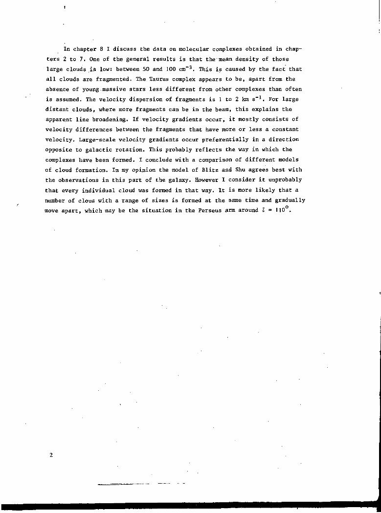
In chapter 8 I discuss the data on molecular complexes obtained in chap-

ters 2 to 7. One of the general results is that the mean density of those

large clouds is low: between 50 and 100 cm"3. This is caused by the fact that

all clouds are fragmented. The Taurus complex appears to be, apart from the

absence of young-massive stars less different from other complexes than often

is assumed. The velocity dispersion of fragments is 1 to 2 km s"1. For large

distant clouds, where more fragments can be in the beam, this explains the

apparent line broadening. If velocity gradients occur, it mostly consists of

velocity differences between the fragments that have more or less a constant

velocity. Large-scale velocity gradients occur preferentially in a direction

opposite to galactic rotation. This probably reflects the way in which the

complexes have been formed. I conclude with a comparison of different models

of cloud formation. In my opinion the model of Blitz and Shu agrees best with

the observations in this part of the galaxy. However I consider it unprobably

that every individual cloud was formed in that way. It is more likely that a

number of clous with a range of sizes is formed at the same time and gradually

move apart, which may be the situation in the Perseus arm around I = 110 .

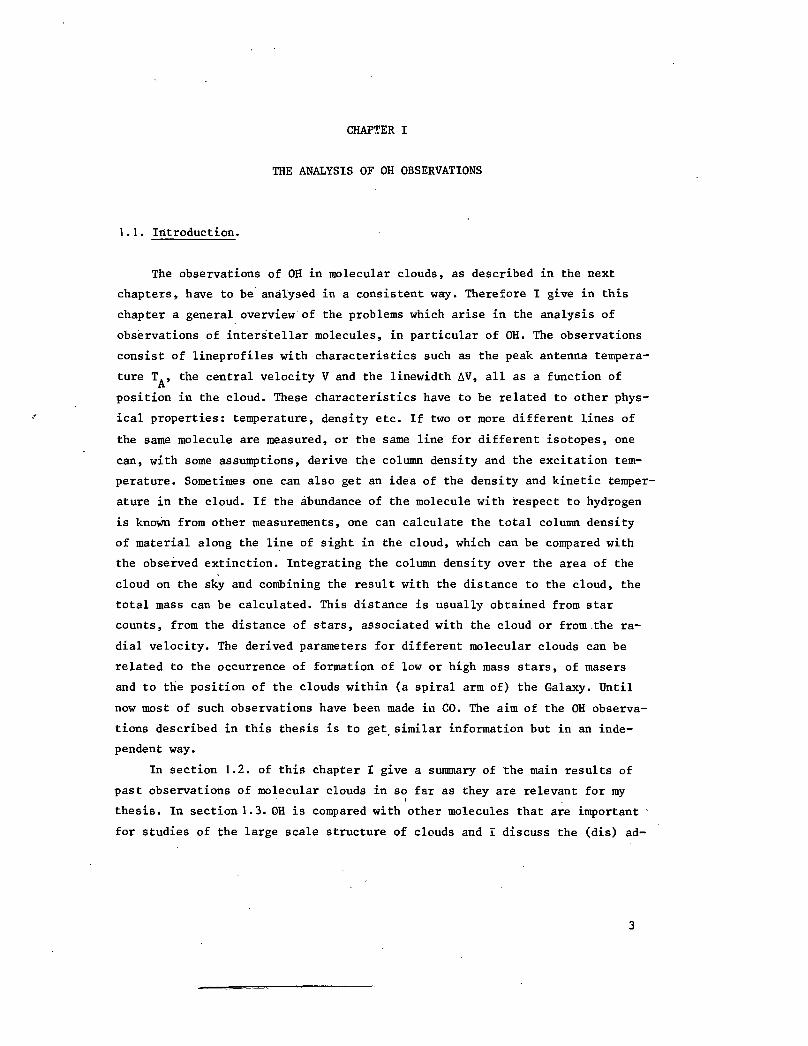
CHAPTER I

THE ANALYSIS OF OH OBSERVATIONS

1.1. Introduction.

The observations of OH in molecular clouds, as described in the next

chapters, have to be analysed in a consistent way. Therefore I give in this

chapter a general overview of the problems which arise in the analysis of

observations of interstellar molecules, in particular of OH. The observations

consist of lineprofiles with characteristics such as the peak antenna tempera-

ture T., the central velocity V and the linewidth AV, all as a function of

position in the cloud. These characteristics have to be related to other phys-

ical properties: temperature, density etc. If two or more different lines of

the same molecule are measured, or the same line for different isotopes, one

can, with some assumptions, derive the column density and the excitation tem-

perature. Sometimes one can also get an idea of the density and kinetic temper-

ature in the cloud. If the abundance of the molecule with respect to hydrogen

is known from other measurements, one can calculate the total column density

of material along the line of sight in the cloud, which can be compared with

the observed extinction. Integrating the column density over the area of the

cloud on the sky and combining the result with the distance to the cloud, the

total mass can be calculated. This distance is usually obtained from star

counts, from the distance of stars, associated with the cloud or from the ra-

dial velocity. The derived parameters for different molecular clouds can be

related to the occurrence of formation of low or high mass stars, of masers

and to the position of the clouds within (a spiral arm of) the Galaxy. Until

now most of such observations have been made in CO. The aim of the OH observa-

tions described in this thesis is to get similar information but in an inde-

pendent way.

In section 1.2. of this chapter I give a summary of the main results of

past observations of molecular clouds in so far as they are relevant for my

thesis. In section 1.3. OH is compared with other molecules that are important '

for studies of the large scale structure of clouds and I discuss the (dis) ad-

ventages of studying each of the molecules. In section 1.4. I summarize our

(limited) knowledge of the excitation mechanisms of the main lines of OH in

molecular clouds and I estimate the expected excitation tpmperatures. In 1.5.

I choose the methodes of analysis of my observations and I summarize this in

1.6.

1.2. Molecular clouds: a summary of known, relevant properties.

Molecules form an important fraction of the mass within the interstellar

medium. This fact became clear mainly as a result of surveys of CO in the

first galactic quadrant (e.g. Burton and Gordon, 1978; Solomon and Sanders,

1980; Cohen et al., 1980). The molecules are concentrated in clouds with wide-

ly varying properties that determine the occurrence of star formation within

the clouds.

There is a large number of parameters and properties of these clouds that

can be obtained from molecular observations. To set the scene for an evaluation

of the observations described in this thesis I will briefly summarize the

present knowledge; I also refer to recent discussions by Evans (1980) and

Turner (1979). One way to analyse the clouds is to look at their properties as

inhabitants of the Galaxy. The clouds have sizes between a few and about hun-

dred pc. Between A and 8 kpc from the galactic center the number of clouds

larger than 10 parsec (sometimes called "giant molecular clouds") is estimated

to be about 4000 (Solomon et al., 1980; Blitz, 1978). The number over the whole

Galaxy will be somewhat higher. In the litterature there is a general agree-

ment about this number and about the mean size of the clouds (25 pc) (Liszt

et al., 1980). However a controversy exists about the distribution of molecu-

lar clouds over the Galaxy. Scoville et al, (1979) concluded from their high

resolution, poorly sampled CO survey of the inner Galaxy that giant molecular

clouds, do not show a significant correlation with the spiral arms, seen in

neutral hydrogen. However a lower resolution CO survey by Cohen et al. (1980)

with a more complete sampling in galactic longitude and latitude shows a

good correlation with spiral structure. Few (1979) observed the same portion

of the galaxy in H„C0 w' th a similar coverage as Solomon et al. in CO. He

concluded cautiously that his results could be conr Lstent with spiral struc-

ture. CO observations of the second galacti; quadrant by Cohen et al. (1980)

showed that there is a contrast in number density of CO clouds of at least a

factor 3 to 5 between the Perseus arm area and the area between the local arm

and the Perseus arm. I obtain the same result in chapter 7 of this thesis.

Cohen's view is supported by the fact that in the solar neighbourhood every

OB association, one of the best indicators of spiral arm structure, is accom-

panied by a large molecular cloud, whereas there appear to be only a few large

molecular clouds without formation of massive stars, although this is observa-

tionally not very firm. I will discuss this point again later in chapter 8.

Finally it is not yet clear to what extent the properties of molecular clouds

in the inner part of the Galaxy are different from the Solar Neighbourhood or

the Perseus arm.

Four cloud properties that are related to each other are the mass, life-

time, formation mechanism and internal structure of the clouds. Solomon et al.

(1980) argue that the mean mass of the clouds is high, about 6 x 105 M_. With

Liszt et al. (1980) these authors are the only ones who published an observed

mass spectrum. This spectrum indicates that an important fraction of the mass

is in clouds with a mass higher than 106 M„. This fraction is not as -large in

the results by Liszt et al. A high mass implies a high mean density, a long

lifetime (longer than 108 years) and the possibility of a relatively slow for-

mation mechanism (coagulation; see Scoville and Hersh, 1979 and Kwan, 1979);

as a consequence the existence is predicted of giant molecular clouds between

the spiral arms. The contrary situation is proposed by Blitz and Shu (1980).

They adopt a five times higher abundance of CO with respect to H» than Solomon

et al. and arrive at a much lower value for the more massive clouds, typically

1 x 105 M_, close to the value of Liszt et al. (1980). One consequence from

Blitz and Shu is that the peak in the molecular hydrogen distribution between

5 and 8 kpc from the galactic center is not as pronounced as in the case of

Solomon et al. Also the mean density within a cloud is then much lower (in the

order of 100 cm"3). To support their views Blitz and Shu add a new indirect

argument: the observations of local clouds show that they have a clumpy struc-

ture. The presence of these clumps indicate a low lifetime (a few 107 years)

because the clumps are bound to coalesce through inelastic collisions. The

lower mass also indicates a shorter lifetime (mass and lifetime are related

through the mean rate of star formation in the Galaxy). Blitz and Shu suggest

that this time is too short to be in agreement with the slow formation through

random coalescence. Some faster way is' required, which can possibly be pro-

vided through Parkers instability within a spiral arm.

The most important internal properties of the clouds consist of the H„

density, temperature, degree of ionisation and the abundances of different

molecules. The H„ density varies from a few times lO-' in areas where 13C0 and

NH_ are.observed, up to 106 cm"3 in the cores of the clouds where for example

the 2 mm lines of H„CO can be detected. The density in the other parts can

only be derived indirectly, from the occurrence of different kinds of mole-

cules. The temperature of most clouds, derived from 12C0 or NH, is about 10 K,

except in regions of active star formation where higher temperatures occur.

The temperature in the outer parts of the low temperature clouds is expected

to be higher than 10 K due to heating by diffuse galactic light. The electron

density is important because for collisional excitation electrons are much

more effective than neutral particles (for OH a factor of 105 is involved).

The most probable value for the fractional ionisation in the cloud cores is

only about 10~8 (Guélin et al. 1977). The value outside the cores is not known,

but presumably it is higher. The abundance of molecules with respect to H„ is

mostly calculated by comparing molecular column densities and column densities

of H2 as derived from extinction measurements using the observed gas-to-dust

ratio in diffuse clouds, N = 2 x I021 A cm"2 (Savage and Mathis, 1979).

Polarization observations suggest that this relation is violated in some

dense molecular clouds where the size of the grains is larger than average

(see e.g. Wu et al., 1980). This effect translates into a larger extinction

per unit mass of interstellar matter and thus a higher molecular abundance

for such clouds.

At present a large number of different molecules is known to exist within

interstellar clouds. A recent list is by Lovas et al. (1979). The molecules

can be divided into a number of groups concerning their abundance at different

densities and the frequencies of their principal lines. Some molecules (e.g.

CH^OCH.., NH.CHO and cyanopolyynes) have only been detected in the cores of a

few clouds. Other, generally simpler molecules are more widely spread. Exam-

ples are NH~ and HCN. Their extent can be traced relatively easily. But be-

cause the transitions are mainly in the mm region, the antenna beam widths are

small and the molecules are only observed in small parts of the cloud. The

transitions are sometimes optically thick in the cloud cores (NH„) and the

observations can be used to estimate temperature and density. But to get in-

sight into the large-scale structure of molecular clouds one needs to consider

with even larger abundances. For this aim the molecules GO, HjCO, CH and OH

are more suitable. They will be discussed in the next section.

1.3. A comparison of CO, H2CO, CH and OH.

1.3.1. CO.

The most widely used lines to map molecular clouds are the 2.6 cm lines

of *2C0 and *3C0. p o r most telescopes this results in a beamsize between 1 and

8 arcminutes; the latter value is for the 1.2 m Columbia telescope in New York.

To map the distribution of CO in nearby clouds with sizes between a few and

more than ten degrees, the small beamsizes result in very long observing times

or in severe undersampling. The exception is the Columbia telescope, with

which telescope the most important CO observations for large-scale investiga-

tions of large clouds have been made (see Blitz, 1980, for a summary of these

observations). Another disadvantage of the line of 12C0 is that it is optically

thick and thus gives information about the kinetic temperature only. To obtain

the CO column density one has to observe also the 13C0 isotope, but then the

line intensities are about a factor 4 lower and accurate observations require

larger integration times. This is the reason why in 13C0 usually one observes

only the cores of the clouds. In the cloud centre 12C0 and 13C0 line intensi-

ties are found to very in proportion and one then assumes that this is also

true for the remainder of the cloud. A puzzle that not yet has been explained

completely satisfactorily is the following: because the 12C0 line is optically

thick, one cannot look very deep into the cloud. Therefore one expects that

the emission does not show much spatial structure. This is not observed. CO

clouds show much structure and resemble observations of lower optical depth

molecules. An explanation for this can be "macro turbulence", a term used for

superposition of individually optically thick fragments with different velo-

cities. Macro turbulence also explains the broad lines (up to 10 km s"1) that

indicate supersonic velocities in molecular clouds (Zuckerman and Evans, 1974).

The three other molecules (OH, CH and H-CO) have lines observable at cm

wavelengths (respectively 18, 9 and 6 cm). Typical antenna beams are conse-

quently larger (3 to 30 arcminutes) so the large-scale structure of clouds

can be obtained more easily. A disadvantage is that the intensities of the

lines are an order of magnitude smaller (typically 0.1 K versus 1 K for CO).

However this is offset by the lower system temperature of the receivers at

cm wavelengths. Compare an OH cloud with T. = 0.2 K, observed with a 30' beam

and a 40 K receiver with 1 km s"1 resolution and a CO cloud of 2 K with an 8'

beam, an 800 K receiver and the same velocity resolution. For a 5cr result the

integration times are 9.9 and 0.6 minutes. If the whole area is mapped in CO

the total observing times required are equal. (However note that this is true

only for the few small CO telescopes available.)

1.3.2. H2CO.

Formaldehyde has transitions at 6 cm, at 2 cm and at mm wavelengths. The

6 cm transition is always seen in absorption, except in two maser sources.

Mapping of clouds is seldomly done; exceptions are the Orion molecular cloud

(Few, 1979) and a southern sky survey (Goss et al., 1980). When only 6 cm

observations are available one needs some assumption for the excitation tempe-

rature (T =1.4 to 2.2 K) to derive column densities. Observations of the

2 cm and of the mm lines are only possible in very small, dense areas of mole-

cular clouds; when available these measurements allow estimates of the local

H„ density.

1.3.3. CH.

The molecular structure of CH is similar to OH with three groundstate

transitions at 9 cm. Absorption measurements have shown that it always is a

very weak maser with excitation temperatures between -20 and -50 K. In most

clouds the CH antenna temperatures are on the average a factor two weaker

than for the OH lines. CH is potentially an important molecule to get addition-

al information about the more diffuse parts of clouds where OH is observed in

the present observations. The CH abundance decreases for densities higher than

about njj = 1000 cm"3 through reactions with 0-atoms. Probably because not

much 9 cm receivers are available at this moment no extensive CH mapping has

been made apart from some limited surveys at Onsala (Rydbeck et al., I976).

However to get observational data on the chemistry of clouds it is important

to observe more clouds in CH.

1.3.4. OH.

The third molecule with ground state transitions at cm wavelengths is OH

(18 cm). The beam sizes of single dish telescopes vary at this wavelength be-

tween 8 and 30 arcminutes which makes OH a very useful molecule to map local

molecular clouds although it cannot be used to observe the smaller scale

structure. After its discovery in 1963 in absorption against Cas A, one first

concentrated at absorption observations (Goss, 1968).

Heiles (1968) was the first to observe thermal emission of OH. Later

(1969) he pointed out a method to calculate the optical depth from the ratio

of the two main line intensities (the meaning of "mainlines" and "satellite

lines1' is explained in section 1.4.). In LTE this ratio varies from 1.8 for

optically thin lines to 1.0 for optically thick ones. Turner and Heiles (1971),

Turner (1973) and Heiles and Gordon (1975) continued to observe in detail a

few selected areas, among others in the Taurus complex (cloud 2) and in

Ophiuchus (cloud 4). Their main conclusion was that the 1665 and 1667 MHz

lines mostly are in LTE, with possibly a few exceptions where a so-called

"mainline anomaly" is present; satellite line anomalies were found to be more

widely spread. Myers (1973 and 1975) mapped parts of some clouds and Crutcher

(1973a) made a survey of OH in dust clouds. The first extensive mapping ob-

servations cf OH clouds are by Sancisi et al. (1974) and by Goss et al. (1976).

They mapped respectively the clouds near the Per 0B2 association and near

NGC 2024. The Per'OB 2 cloud was the first with a more detailed investigation

of the variation of the ratio of the mainlines over a large part of the cloud.

Correlations of OH with H I, H-CO and optical extinction were made for

some clouds in the Taurus area, in Perseus 0B2, in Khavtassi 3 and in L 134

(Turner and Heiles, 1974; Sancisi et al., 1974; Myers, 1975; Mattila et al.,

1979). With the exception of Khavtassi 3 in all clouds the OH antenna temper-

ature appears to be positively correlated with extinction if a low optical

depth for OH is assumed. Usually there is a weak correlation of OH and H2C0

antenna temperatures. No detailed investigation of a correlation between OH

and CO has been made, except for the L 134 cloud (Mattila et al., 1979). Baud

and Wouterloot (this thesis, chapter 2) made a low sensitivity OH survey of

large molecular clouds in Taurus and Orion. This survey confirmed the earlier

result of Sancisi et al. that molecular clouds can be equally well be mapped

in OH as in CO; it was the basis to start the more extended program of OH

observations described in this thesis.

1.4. OH excitation.

The rotational levels in the energy spectrum of OH are relatively widely

spaced. The first excited rotational levels (2ïïi, J = •=- and 2ir^, J = •*•) are

Figure 1.1.

The energy levels of the 2v$, J = -~ ground state of OH

drawn to scale. Transition c •*• b aorresponds to the200 MHz

1 1612 MHz 3 e + a to the 1665 MHz3 d •+ b to the 1667 Misand d •*• a to the 1720 MHz line.

o

at 84 and 126 cm"1 above the 2iT3, J = y ground state. Therefore in cold molec-

ular clouds most OH molecules will be in the ground state. This state is split

up into two levels due to A doubling and each A-doublet level is once again

split due to hyperfine structure (see figure 1.1. which is drawn on scale).

Four transitions are possible: the "main lines" at 1665 MHz (c -*• a) and 1667

MHz (d -> b) and the "satellite lines" at 1612 MHz (c ->- b) and 1720 MHz (d -> a).

In a first approximation the excitation of each of the main lines can be de-

scribed by a two level model (Rogers and Barrett, 1968)

T + TTeTTex,i

where T is the excitation temperature, T the background radiation temper-6X IJ\3

ature and Tv the kinetic temperature. The index i indicates the line numberis.

i = 1 (1612 MHz), i = 2 (1665 MHz), i = 3 (1667 MHz), i = 4 (1720 MHz). T .u,i

is the ratio between collisional de-excitation and spontaneous emission

across the transition. Theoretical arguments suggest (but do not prove) that

I. „ % T. „. and that it is given by the following relation (Guibert et al.,

1978)

0,1 k A. K

Here A. is the spontaneous transition rate and C the collisional de-excitation

rate. Inserting A- = Ao = 7.5 x 10"11 and assuming a value C = 6.7 x- 10~12

cm"3 s"1 for collisions with H, molecules they obtain Tn , = 7 x 10~3 n .T 2,

where n is the density óf hydrogen molecules. The satellite lines are easily

10

influenced by collisional and radiative transitions to other levels (Elitzur,

1978) so that (1.1) holds only for the main lines. Several possible modifica-

tions for equation (1.1) might be considered. Firstly Kaplan and Shapiro

(1979) calculated the transition rates for collisions with H-atoms. If their

result is applied to (1.2), T n . is different for the two main lines. Thisu,i

creates a difference in excitation temperature DT (= T „ - T ,) of a few

times 0.1 K for T = 10 K and n = 1000 cm"3. However, since excitation by H.

molecules is far more important it is questionable whether Kaplan and Shapiro's

result is applicable. Secondly, equation (1.2) has to be modified if the frac-

tional ionisation (n /n) exceeds 10~5, because electron collisions then start

to dominate over collisions by H„ molecules (Guibert et al., 1978). However

the fractional ionisation in the cloud cores is currently thought to be low

(10~7 - 10~8). Thirdly, Gwinn et al. (1973) proposed an excitation mechanism

involving collisions to the excited 2TT3 J = y and 2ITJ_ J = y states of OH. Then

equation (1.1) has to be modified to (Dickey et al., 1981)

where T and T~ are defined as T_ in equation (1.2), but with C referring to

the specific collisional excitation rates of the two excited states. These

rates are known with so little precision that it is of no use to distinguish

the two main lines. If the rates guessed by Turner (1973) are adopted (C. =

1.0 x 10"11 n T.} exp (-120/X) and O, = 1.0 x 10"11 n T_^ exp (-184/T ))Is. K Z K K

then collisional transitions via these excited states become important for

n(H_) > 1000 cm"3 and T > 10 K. However if the cross sections for collisions

with H^ molecules are as small as calculated by Kaplan and Shapiro (1979) for

H atoms (about 10 times smaller) the Gwinn et al. process would be only impor-

tant in dense cloud centers. In practice the choice between equation (1.1)

and (1.3) can be avoided because in all cases of interest T. and T„ are much

smaller than T_ so that equation (1.3) reduces to equation (1«O.

It is possible that some of the infrared transitions towards rotationally

excited states are optically thick. This, together with overlapping lines due

to velocity gradients can cause a difference in the excitation temperature of

the main lines (Bujarrabal and Nguyen-Q-Rieu, 1980). This effect is very sen-

sitive to the line broadening mechanism and to the magnitude of the linewidth

11

of the OH lines.

Guibert et al. (1978) have made a detailed calculation of the excitation

of the satellite lines. They showed that these lines can be more indicative

of the special circumstances in molecular clouds than the main lines. Because

of the many parameters which enter their calculations (density, temperature,

degree of ionisation, grain temperature T , dilution factor W, OH column den-

sity), it is difficult to summarize their results in a few words. Under typi-

cal circumstances in the observed clouds (n = 100 to 5000 cm"3, T_ = 5 to 15 K,

n /n„ + nH = I0~7 to 10"8, I. = 5 to 15 K, H < )0~h, NrtTI = 1014 to 1015 cm"2

e n a2 " "" Unand N „/AV = 3O~2 to 10~3 cm~3 pc km"1 s), a positive value of T . is ex-

un ex,ipected. The predicted values of T , and T _ are somewhat smaller. Since

ex,^ ex,j

the predicted value of T . is approximately equal to T__, the 1612 MHz line

can be seen either in weak emission or in weak absorption. T , is probablylarger than T . and T ,; it may even become inverted. Therefore the 1720

ex,^ ex, .5MHz line is expected to be seen in relatively strong emission.

1.5. The analysis of the observations.

1.5.1. Excitation temperatures, optical depths and column densities.

The measured parameters T. . and AV. of the observed transitions have to

A, 1 1

be related to the following physical parameters: the total OH column density

N_„, the excitation temperature of the observed line T . and the volumeUli 6Xy 1

density n of H*. In general for each measured line there are two equations

TA,i - V ( T e x , i " V O - e ) O-*-)

N0H " Ci Tex,i AVi Ti °- 4 b )

where nB is the beam efficiency (0.76 for the Dwingeloo celescope), F the

filling factor (i.e. the fraction of the beam size filled by the gas), T. the

; optical depth at the line center and C- a constant ( 22.21, 4.30, 2.39 and

' 20.82) x lO14 cm2 K"1 km"1 s for i = 1 to 4).

Since the satellite lines are always very weak, often only the 1665 and

j 1667 MHz lines are measured. I consider this case first. Then there are 2

-I

12

Ifl -

QO 0.1 02 O.I. 0.6 0.8 1.0 2.0 3D 40 Sfl

13 —2Figure 1.2. Lines of constant OH column density (in units of 10 am ) as a

function of R and VT for TA 3 = 0.3 K, F= 1.0, LV = 1.0 hn s'1

and T^n = 3.2 K.BG

sets of 2 equations (1.4) with 5 unknowns: T „, T ,, x , T, and N and 5

quantities that are directly measured: T. „, T _, T , AVO and AV_. In general

F is also unknown, but it is probably equal for the two main lines and in most

cases it i as a first approximation put equal to 1. To derive values for the

5 unknowns we have to make some extra assumption. For that purpose I introduce

the parameter, DT = T „ - T ,. Often DT is assumed to be zero, i.e. T6X y £• 6X y J GX 9 £,

= T , (see the discussion in section 1.3.A.). In that case the ratio6X 9 J

R = T /T is between 1.8 and 1.0. Theoretically (section 1.4) DT may have

values significantly different from zero, although the conditions are probably

not easy to create. If a continuum radio source is situated behind the molec-

ular cloud, the two excitation temperatures, T , and T _ can be derivedex, i. ex, j

from absorption measurements. Such observations show (Dickey et al., 1980)

that small excitation temperature differences (DT < 1 K) do exist. One of the

best known cases is 3C 123 (Nguyen-Q-Rieu et al., 1976), where DT = 1 to 2 K.

Crutcher (1979) argues that main line anomalies are rather wide-spread, but

his observations are too few and not sufficiently accurate to accept his con-

clusions as certain. Actually I have-concluded that main line anomalies are

rather unimportant (see the next chapters). In the rest of my thesis I assume

that DT is 0, although I often will indicate how my conclusions change if this

assumption is not correct. Quite generally, for a given value of N_„ an in-

13

creasing positive value of DT results in a decrease of R and an apparent in-

crease in TO. As an illustration I show in figure 1.2. N_u as a function of DT

and of R. Since R is a measured quantity, one notices the uncertainty in N-,,

by moving horizontally in figure 1.2. and the variation in N _ . The calculationUfi

was made for T. , = 0.3 K (nR = 0.76), a filling factor F = 1.0, a linewidth

AV = 1.0 km s"1 and a background radiation temperature T „ = 3.2 K. Figure 1.2.

shows that at R = 1.5, N.„ changes from 3 * I015 cm"2 (DT = -0.1) via 1-x 1015

Url

cm"2 (DT = 0) to about 2 x lO14 cm"2 (DT = 1.0). It can be concluded that the

influence of DT is largest for small DT. If DT is larger than 5 K, the varia-

tion of Nrt with DT becomes negligible. Diagrams (not shown) have also beenUn

made of T _ and of T O as a function of DT and R. The line of constant N.,T =ex,3 3 OH

1.5 x 1014 cm"2 in figure 1.2. corresponds nearly with a line of constant

T , = 10 K. In this way one can, if a most probable value of T _ in molec-

ular clouds is derived in some way, obtain an upper limit for DT. However be-

cause, as figure 1.2. shows, the major influence of DT on N_ occurs for smallUn

values of DT, this does not diminish the uncertainty in N_„ much. A lowerUn

limit for the column density can be obtainec fromC. AV. Tx 1 e

N = x 1 e x» 1

0 H F " B T e x i -

which is the limit of equation (1.4b) in the case of small optical depths. In

many cases the factor T /(T - T ) is omitted. However observations of OHex ex o\s

in emission and absorption in diffuse clouds in front of extragalactic radio

sources (Dickey et al., 1980) show that this factor can become as high as 3.0

and I will adopt T = 5.5K in the next chapters. Equation (1.5) can also be

used if To > 0 if it is multiplied with a factor

f = ƒ i ' (v) dv / ƒ Q - exp (- T ' (v))3 dv, where T ' (v) has a Gaussian

line profile (see Mattila et al., 1979). The result is then identical with

that of Equation (1.4b).

If observations of all four 18 cm OH lines are made, an essentially bet-

ter method of analysis is available, that appears to have been used first by

Mattila et al. (1979). In this case one has four sets of two equations (1.4).

But there exists an additional ninth equation, the strictly valid sum rule,

0*6)

14

so that in total there are 9 equations with 9 unknowns. F is still unknown,

but I will assume that it is equal for all four lines. The set of nine equa-

tions can be solved in the following way. For a given, most probable value of

F, and for some adopted DT the observations of the main lines give values for

the column density N„TT, for T ' o and thus for T „ = T „ + DT. Then' OH' ex3 2 x 3OH' for T ' o and thus for T „ = T „ + DT.

ex,3 ex,2 ex,3.equation (1.6) still allows a series of combinations (T ., T , ) , each

ex f I cX y *iof which predicts specific values of T, . and T. , via equations (1.4).

Comparing the predicted values T. ., T. , with those actually observed I

find the correct values of T , and T .. Because theoretically and

observationally there is only a limited range for T ., and DT the number€X } -J

of combinations (T ., T ,) which has to be investigated is limited. IneX y 1 eX y H-

this way Mattila et al. (1979) concluded that in the L134 cloud a positivevalue for DT is likely. The method does not give values for T . and T

ex 9 j e

all cases, especially not when T, is small.

1.5.2. Abundance s.

Tex j

in

Once values of N n u, T. and T „ have been obtained in the way describedKJtt J e x y j

in the previous section, they can be combined with other parameters of the

clouds, such as the total (i.e. molecular plus atomic) hydrogen column density

N (derived from the visual extinction A^, Savage and Mathis, 1979) or a

Figure 1.3. Chemical reaction scheme fov the production and destruction of OH.

Important reactions in the outer parts are drawn as dashed lines.

The other ones dominate in the cloud center.

15

mean density obtained either by dividing N by some dimension of the cloud

or from a combination of equations (1.1) and (1.2). Knowledge of N is nec-

essary if one wants to estimate the mass of the cloud. Also the abundance of

OH, the ratio N_ /N , is interesting from various points of view. In analy-Un coc

sing the excitation temperatures and other parameters one has to keep in mind

that these values are an average along the line of sight through the cloud.

Presumably variations of T with depth in the cloud occur.

The OH abundance can be obtained either theoretically or observationally.

Theoretically the abundance can be obtained from chemical equilibrium calcula-

tions. The formation and destruction reactions of OH are drawn schematically

in figure 1.3. The reactions indicated by dashed lines are more important in

the outer parts of the cloud, where UV photons are present. The others domi-

nate in the center of the cloud, where cosmic rays are present. An equilibrium

state will be achieved in times of the order of 10^ year, which depends on

density, temperature, ÜV flux and cosmic ray ionisation flux. For purposes of

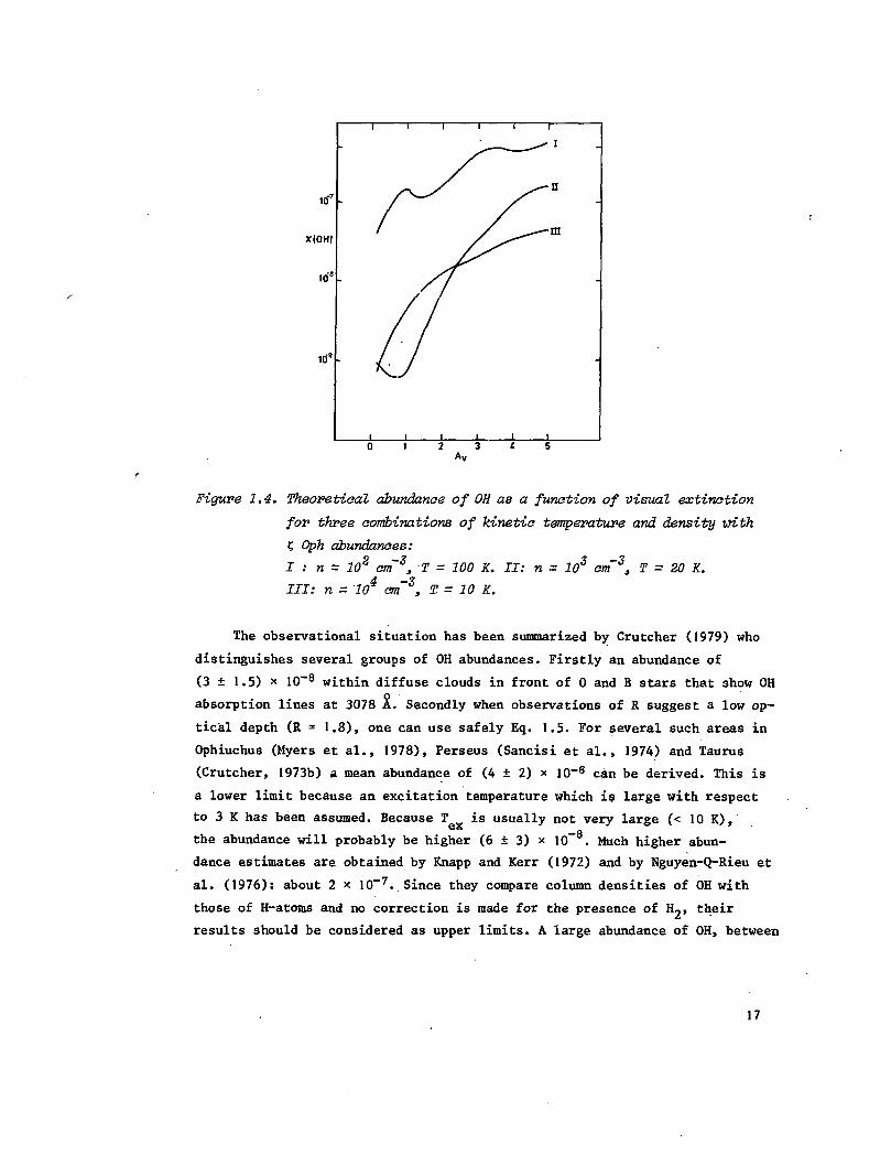
illustration I display some results in figure 1.4. Details of the calculations

are given elsewhere (Tielens and Hagen, 1981). Figure 1.4. shows that the OH

abundance can vary between 10"^ and a few time 10~7, with the higher abundances

at higher values of the extinction. A more realistic cloud model requires a

combination of such calculations because in the cloud center the density will

be higher and the temperature lower. So probably this causes a transition from

curve 1 in the outer part of the cloud to curve 3 in the cloud center. Accord-

ing to these calculations the abundance ranges from 10~8 to 10~7. Calculations

of cloud models with varying temperature and density have been made by de Jong

et al. (1980). They find OH abundances that are a factor 10 smaller than those

in figure 1.4. This is the typical uncertainty in theoretical abundances that

arises because it is dependent on so many parameters. Viala et al. (1979)

arrive at similar values, which can increase if OH formation on grains is in-

cluded. The values in figure 1.4. were obtained for atomic abundances found

for the cloud in front of ? Oph. The OH abundance strongly depends on the

adopted metal abundance because the metal abundance governs the degree of ioni-

sation, which is an important factor in the formation of OH. Another uncertain-

ty is the photodissociation rate of ÖH. Recent calculations by Ms. E. van

Dishoeck (private communication) show it to be a factor 3 higher than those

used for figure 1.4., which is important in the outer parts of the cloud. At

this time theoretical abundances are not yet accurate enough to use in the

derivation of cloud masses.

16

10"7

XIOHI

10»

ie*

I I I

I

" /1I I I

1 > 1

-

1 1 1

2 3Av

Figure 1.4. Theoretical abundance of OH as a function of visual extinction

for three combinations of kinetic temperature and density with

t, Oph abundances:

I : n = 102 cm'3. T = 100 K. II: n = 103 erf3. T = 20 K.

Ill: n = 104 cm'3. T. = 10 K.

The observational situation has been summarized by Crutcher (1979) who

distinguishes several groups of OH abundances. Firstly an abundance of

(3 ± 1.5) x 1O~8 within diffuse clouds in front of 0 and B stars that show OH

absorption lines at 3078 A. Secondly when observations of R suggest a low op-

tical depth (R = 1.8), one can use safely Eq. 1.5. For several such areas in

Ophiuchus (Myers et al., 1978), Perseus (Sancisi et al., 1974) and Taurus

(Crutcher, 1973b) a mean abundance of (4 ± 2) * 10~8 can be derived. This is

a lower limit because an excitation temperature which is large with respect

to 3 K has been assumed. Because T is usually not very large (< 10 K ) ,e X -8

the abundance will probably be higher (6 ± 3) x 10 . Much higher abun-

dance estimates are obtained by Knapp and Kerr (1972) and by Nguyen-Q-Rieu et

al. (1976): about 2 x 10~7. Since they compare column densities of OH with

those of H-atoms and no correction is made for the presence of H„, their

results should be considered as upper limits. A large abundance of OH, between

17

1.5 and 3.5 x ]0~7 is found in an area in Taurus with a large apparent optical

depth T. (Turner and Heiles, 1974). This abundance is consistent with a theo-

retical value at high densities and A (see figure 1.4.). The conclusion holds,

however, if DT < 0.1. Otherwise NQ„ will be smaller (see figure 1.2.), and the

abundance will be the same as in low optical depth areas.

It is obvious that the abundance of OH is quite uncertain. To calculate

the total H column density from the OH observations there are two possibili-

ties, of which I prefer the second. Firstly, as Crutcher (1979) proposed, to

use everywhere an abundance of 4 x IO~8 (or 6 x 10~8 if corrected for a lower

excitation temperature than he used), assuming that main line anomalies are

common in OH clouds, and that the large apparent abundances in the Taurus

clouds are the result of the assumption DT = 0. Secondly, to assume that

DT = 0 (or very small), because several observations, presented in the next

chapters do suggest this, and to accept the theoretically supported fact that

the abundance varies with optical depth. Therefore I will use an abundance of

2 x 10~7 at high optical depths (x- = 2) and 6 x 10~8 at x- = 0. Because a

jump in abundance is improbable I propose the following relation between T-J

and the abundance:

NOH/Ntot " (7 T3 + 6 ) * 10'8 ( K 7 )

for 0 < T- < 2. If T_ > 2, which seldom occurs I shall use a constant abun-

dance of 2 x 10~7. This resembles all theoretical calculations (Viala et al.

1979) where the abundance increases until a certain depth in the cloud and

stays more or less constant thereafter (see also figure 1.4.). Equation (1.7)

can still be used if at some position DT f 0 because in that case x„ = 0

(Crutcher) is a too extreme assumption.

1.6. Procedure adopted to analyse the observations.

In this section I give a summary of the way in which the analysis of the

observations, described in the chapters 3 to 7 will be made. In all clouds

only the two main lines were measured over the whole cloud area. In most clouds

I made observations of the satellite lines at a few positions with high main

line antenna temperatures. So a detailed analysis of the OH properties as

described in section 1.5.1. is for most clouds possible but only, in a few

18

positions. Nevertheless it gives important additional information. In the rest

of the cloud I will make a statistical analysis of the main line properties in

regions where the excitation conditions probably are the same. In this case

there are two possibilities. Firstly R - 1.8, which means T, « 1 so that I

can use eq. (1.5) to obtain N_ . The main uncertainties are the filling factor

and the excitation temperature. Secondly, R < 1.8, which includes two possibi-

lities: a. DT = 0 and T, is substantial, b. DT f 0 and T_ is small. To see if

a. or b. is valid I will use other data such as (i) satellite line measure-

ments in the concerning part of the cloud, (ii) absorption measurements of the

main lines against continuum sources, or (iii) extinction measurements and the

probable relation T./abundance. Then I can obtain N Q H via eq. 1.4.b using the

most probable F. In the case of a high T_ I use eq. (1.1) to obtain a crude

estimate for the density. Then N is calculated from N , using eq. (1.7)

and the total mass of the cloud can be derived by integrating over the cloud

area.

References.

Blitz, L., J980, in: Giant molecular clouds in the galaxy, ed. P.M. Solomon

and M.G. Edmunds (Pergamon Press).

Blitz, L.s Shu, F.H., 1980, Astrophys. J. _238, 148.

Bujarrabal, V., Nguyen-Q-Rieu, 1980, Astron. Astrophys. 9J_, 283.

Burton, W.B., Gordon, M.A., 1978, Astron. Astrophys. 63, 7.

Cohen, R.S., Cong, H., Dame, T.M., Thaddeus, P., 1980, Astrophys. J. 239, L53.

Crutcher, R.M., 1973a, Astrophys. J. 185, 857.

Crutcher, R.M., 1973b, Astrophys. Lett. J4_, 147.

Crutcher, R.M., 1979, Astrophys. J. 234, 881.

De Jong, T., Dalgarno, A., Boland, W., 1980, Astron. Astrophys. 9±, 68.

Dickey, J.M., Croviiier, J., Kazès, I., 1981, Astron. Astrophys. 98_, 271.

Elitzur, M., 1978, Astron. Astrophys. ji2, 305.

Evans II, N.J., 1980, in: Interstellar Molecules, ed. B.H. Andrew, (Reidel) p.l,

Few, R.W., 1979, Month. Not. R.A.S. 2£7, 161.

Goss, W.M., 1968, Astrophys. J., Suppl. J_5> 131>

Goss, W.M., Winnberg, A., Johansson, L.E.B., Fournier, A., 1976, Astron. Astro-

phys . jij6, 1.

19

Goss, W.M., Manchester, R.N., Brooks, J.W., Sinclair, M.W., Manefield, G.A.,

Danziger, I.J., 1980, Month. Not. R.A.S. 2£i» 533*

Guélin, M., Langer, W.D., Snell, R.L., Wootten, H.A., 1977, Astrophys. J.,

217, L165.

Guibert, J., Elitzur, M., Nguyen-Q-Rieu, 1978, Astron. Astrophys. jj6_, 395.

Gwinn, W.D., Turner, B.E., Goss, W.M., Blackman, G., 1973, Astrophys. J. 179,

789.

Heiles, C , 1968, Astrophys. J. _T51̂ 919.

Heiles, C , 1969, Astrophys. J. 257., 123.

Heiles, C , Gordon, M.A., 1975, Astrophys. J. _ljJ9, 361.

Kaplan, H., Shapiro, M., J979, Astrophys. J. 229, L91.

Knapp, G.R., Kerr, F.J., 1972, Astron. J. 7J_, 649.

Kwan, J., 1979, Astrophys. J. 229, 567.

Liszt, H.S., Xiang, D., Burton, W.B., 1980, preprint.

Lovas, F.J., Snyder, L.E., Johnson, D.R., 1979, Astrophys. J. Suppl. ̂ 1_, 45J.

Mattila, K., Winnberg, A., Grasshof f, M., 1979, Astron. Astrophys. 2s., 275.

Mitchell, G.F., Ginsburg, J.L., Kuntz, P.J., 1978, Astrophys. J. Suppl. 38, 39.

Myers, P.C., 1973, Astrophys. J. Suppl. ̂ 6, 83.

Myers, P.C., 1975,. Astrophys. J. 198, 331.

Myers, P.C., Ho, P.T.P., Schneps, M.H., Chin, G., Pankonin, V., Winnberg, A.,

1978, Astrophys. J. J22O, 86^-

Nguyen-Q-Rieu, Winnberg, A., Guibert, J., Lépine, J.R.D., Johansson, L.E.B.,

Goss, W.M., 1976, Astron, Astrophys. 4̂6, 413.

Rogers, A.E.E., Barrett, A.H., 1968, Astrophys. J. J51, 163.

Rydbeck, O.E.H., Kollberg, E., Hjalmarson, A, Sume, A., Ellder, J., Irvine,

W.M., 1976, Astrophys. J. Suppl. 2I1_, 333.

Sansici, R., Goss, W.M., Andersson, C , Johansson, L.E.B., Winnberg, A., 1974,

Astron. Astrophys. J35_, 445.

Savage, B.D., Mathis, J.S., 1979, Ann. Rev. Astron. and Ap. ̂ Z» 73'

Scoville, N.Z.., Hersh., K., 1979, Astrophys. J. _229, 578.

Scoville, N.Z., Solomon, P.M., Sanders, D.B., 1979, in: The large-scale charac-

teristics of the galaxy, ed. W.B. Burton (Reidel) p.277.

Solomon, P.M., Sanders, D.B., 1980, in: Giant Molecular Clouds in the Galaxy,

ed. P.M. Solomon and M.G. Edmunds (Pergamon Press).

Tielens, A.G.G.M., Hagen, W., 1981, in preparation.

Turner, B.E., 1973, Astrophys. J. 186, 357.

20

Turner, B.E., 1979, in: The large-scale characteristics of the Galaxy, ed.

W.B. Burton (Reidel),

Turner, B.E., Heiles, C , 1971, Astrophys. J. 170, 453.

Turner, B.E., Heiles, C , 1974, Astrophys. J. ̂ 94, 525.

Viala, Y.P., Bel, N., Clavel, J., 1979, Astron. Astrophys. 22.t 174.

Wu, C C , Gilra, D.P., Duinen, R.J. van, 1980, Astrophys. J. 241, 173.

Zuckerman, B., Evans II, N.J., 1974, Astrophys. J. 22£,

21

Astron. Astrophys. 90, 297-303 (1980) ASTRONOMYAND

ASTROPHYSICSCHAPTER I I

OH Observations of Molecular Complexes in Orion and Taurus

B. Baud1-2 and J. G. A. Wouterloot'1 Sterrewacht, Postbus 9513, NL-2300 RA Leiden, The Netherlands2 Radio Astronomy Laboratory, University of California, Berkeley, CA 94720, USA

Received November 29, 1979; accepted February 28,1980

Summary. The molecular complexes in Orion and Taurus havebeen mapped in both OH main lines over a large (£20°x20°)area of sky in order to trace out their full extent. The derivedcolumn density and total mass of the complexes are in goodagreement with CO results.

The molecular emission in Orion is embedded in a large HIcomplex, that extends 200 pc below the plane. The Orion A and Bcomplexes lie at the edge of this Hi complex, defining a sharpboundary between gas and dust rich and poor regions. Starformation efficiency in Orion is 5-10%.

The Taurus molecular complex is surrounded by small clouds.Coagulation of these small clouds could belance the present gasdepletion rate due to the low rate of star formation. However,formation of an OB association would destroy the molecularcomplex in 107 yr.

Key words: OH emission - molecular clouds - star formation -Orion - Taurus

I. Introduction

It now appears to be an established fact that OB associations inthe solar neighborhood are associated with giant molecular com-plexes (Kutneretal., 1977; Blitz, 1978; Sargent, 1977,1978; Elme-green and Lada, 1979). CO observations of these complexes showhighly lumpy structures, usually elongated over 60-100 pc, oftenextending over large areas of sky.

The 18 cm OH mainlines are potentially excellent tracers forthese local molecular complexes. The usually large telescope beamof several tens of arc min allows for relatively fast mapping of largeareas of sky, while data at both mainlines can provide informationon the optical depth and yield an independent mass estimate of thecomplexes.

In this paper we present the results of a low S/N OH survey ofthe star-forming regions in Orion and Taurus, covering more than200 square degrees in each case.

Large scale OH emission associated with the well known giantcomplexes was found both in Orion and in Taurus. In the caseofOrion no other molecular complexes were found up to 20° distancefrom the Orion HII region. The survey coverage in Taurus wasnot sufficient to map the full extent of the molecular emission.

Send offprint requests to: J. G. A. Wouterloot

Small isolated clouds were detected near the big complexes.The structure of the OH emission is compared with the large

scale HI and CO emission and the extinction. The efficiency ofstar formation and its velocity through the Orion A molecularcomplex are discussed. In addition the cloud coagulation rate iscompared to the gas depletion rate due to star formation.

II. Observations

The observations were done with the 25 m Dwihgeloo telescope ina total power mode on a rectangular grid of positions in / and b.Separation between grid points was 0:3, corresponding to 2/3 ofthe half-power beam width {HPBW=31'}.. The single channelcooled paramp receiver had a system temperature of 45 K on coldsky. The 1665 MHz and 1667 MHz lines were observed simultan-eously by splitting the 256 channel autocorrelator into equal hal-ves, each with a bandwidth of 1.25 MHz. Velocity coverage ineach line was 225 km s"1 centered on 1^,.= +20 km s"1 forOrion and —60 km s~' for Taurus. With an integration time of5 min per grid point and a spectral resolution of 11.7 kHz (2.1 kms " ' ) a rms sensitivity of 0.05 K. antenna temperature was obtained.The beam efficiency was 0.75.

For each position both spectra were plotted after subtractionof a linear baseline. Any features larger than 5 a, or weaker signals(S2<r) occurring in neighboring positions or in both lines at thesame velocity, were considered real.

in . Orion

1. Results

New OH clouds found in the region around Orion (Fig. 1) arelisted in Table 1. The position refers to the indicated maximumantenna temperature. The corresponding radial velocity is withrespect to l.s.r. Since all emission sources were extended or inrough agreement with optically thin LTE conditions [7^(1667)/7^(1665)» 1.8 — 1.4] we conclude that no new masers were found.

The distribution of the 1667 and 1665 MHz emission andabsorption is shown in Figs. 2a and 2b. Because the 1665 MHzemission of many clouds was below the detection limit we willconcentrate our discussion on the 1667 MHz map. The most out-standing features of the molecular complex morphology are thefollowing.

1. A molecular ridge running at a 45° angle with respect to thegalactic plane from L 1617 via NGC 2071 and NGC 2024 down

23

298

i—IJ

J

L-

-25.0 -

JfYOri

III

1

r~i

Ii

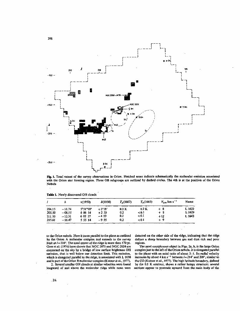
I

Fig. 1. Total extent of the survey observations in Orion. Hatched areas indicate schematically the molecular emission associatedwith the Orion star forming region. Three OB subgroups are outlined by dashed circles. The 4th is at the position of the OrionNebula

T«Me 1. Newly discovered OH clouds

/ a(1950) (5(1950) ^(1667) ^(1665) km s" Name

204.15205.50211.50215.81

-11.74-08.15- 1 2 . 3 1- 1 6 . 4 7

5h51mO3'6 06 146 02 275 55 14

+ 2°18'+2 50- 4 19- 9 55

0.2 K0.20.20.2

0.2 K + 8+ 8+ 12+ 9

L1622L1629L1643

to the Orion nebula. Here it turns parade] to the plane as outlinedby the Orion A molecular complex and extends to the surveylimit at /=216°. The total extent of the ridge is more than 170 pc.Goss et al. (1976) have shown that NGC 2071 and NGC 2024 areconnected on 'the sky by a bridge of low surface brightness OHemission, that is well below our detection limit. This emission,which is elongated parallel to the ridge, is associated with L 1630and is part of the Orion B molecular complex (Kutner et al., 1977).

2. Several smaller OH clouds at similar velocities were foundlongward of and above the molecular ridge while none were

detected on the other side of the ridge, indicating that the ridgedefines a sharp boundary between gas and dust rich and poorregions.

The most conspicuous object in Figs. 2a, b, is the large Orioncomplex just to the left of the Orion nebula. It is elongated parallelto the plane with an axial ratio of about 3:1. Its radial velocityincreases by about 4 km s~' between /=214° and 209°, similar tothe CO (Kutner et al., 1977). The high latitude boundary, definedby the 0.1 K contour, shows a rather lumpy structure: several

sections appear to protrude upward from the main body of the

24

B. Baud and J. G. A. Wouterloot: Molecular Complexes 299

213° 2»" 207° 204° 201° X

Fig. 2a aatf b. Distribution of the peak antennatemperature in Orion at 1667 MHz a and1665 MHzb. Radial velocities with respect tol.s.r. are indicated in km s~'. Emission contoursare continuous; absorption is dashed. Minimumcontour value 0.1 K; contour interval is 0.1 K,( x ) is maser emission. For easy comparisonwith other species the molecular ridge is shownschematically as a shaded line; ( ) showsthe survey extent

complex, pointing towards NGC 2024 and the small clouds justabove at + 6 and + 4 km s~'. The latter may well be physicallyconnected to the Orion A complex by low-level emission similarto that found by Goss et al. (1976) around NGC 2071 and 2024.Around the Orion nebula, the emission is not shown because theline profiles are dominated by strong absorption against the radiocontinuum from the H n region (Fig. 2a) or the maser emission(Fig. 2b).

Due to the low OH optical depth only about half of the otherclouds in the field were detected at 1663 MHz.

2. Discussion

a) The Molecular Ridge

The presence of a sharp boundary between molecular rich andmolecular poor regions in Orion, as defined by the molecular

ridge, is supported by the following evidence: (i) The more sen-sitive OH observations of L 1630 at Orion B by Goss et al. (1976)show that the emission drops off steeply shortward of the emissionmaximum at NGC 2071 and NGC 2024, while low-level emissionappears to extend to several degrees longward of these maxima,(ii) A similar phenomenon is apparent from the CO map by Kutneret al. (1977), reproduced in Fig. 3. The CO emission from theOrion A complex shows a sharp lower boundary, which is coin-cident with the OH boundary. The upper boundary of the COemission has a more irregular shape, analogous to the OHemission. In Orion B the CO emission also shows a sharp edgeshortward of the emission peaks at NGC 2071 and NGC 2024and more extensive low-level emission at larger longitudes, (iii)Both the large scale HI emission (Fig. 4a) and the visual extinction(Fig. 4b) show a distribution analogous to the molecular ridge.Inspection of the high-latitude Hi survey by Heiles and Habing(1974) in Fig. 4a (peak antenna temperature between 4.8 and6.9 km s"') shows strong (7],%40 K) Hi emission that extends

25

.20° -

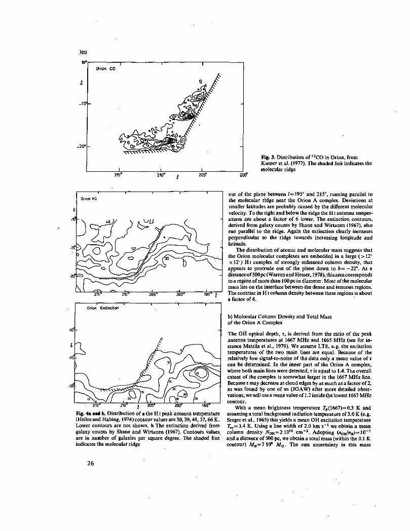
215'

Fig. 3. Distribution of 12CO in Orion, fromKulner et al. (1977). The shaded line indicates themolecular ridge

215" 210" 205° 200" 195

Fig. 4a and b. Distribution of a the HI peak antenna temperature(Heiles and Habing, 1974)contour values are 30,39,48, 57,66 K.Lower contours are not shown, b The extinction derived fromgalaxy counts by Shane and Wirtanen (1967). Contours valuesare in number of galaxies per square degree. The shaded lineindicates the molecular ridge

out of the plane between /=195° and 215°, running parallel tothe molecular ridge near the Orion A complex. Deviations atsmaller latitudes are probably caused by the different molecularvelocity. To the right and below the ridge the HI antenna temper-atures are about a factor of 6 lower. The extinction contours,derived from galaxy counts by Shane and Wirtanen (1967), alsorun parallel to the ridge. Again the extinction clearly increasesperpendicular to the ridge towards increasing longitude andlatitude.

The distribution of atomic and molecular mass suggests thatthe Orion molecular complexes are embedded in a large (> 12°x 12°) Hi complex of strongly enhanced column density, thatappears to protrude out of the plane down to b= -22° . At adistanceof 500 pc (Warren and Hesser, 1978), thisarea correspondsto a region of more than 100 pc in diameter. Most of the molecularmass lies on the interface between the dense and tenuous regions.The contrast in HI column density between these regions is abouta factor of 6.

b) Molecular Column Density and Total Massof the Orion A Complex

The OH optical depth, T, is derived from the ratio of the peakantenna temperatures at 1667 MHz and 1665 MHz (see for in-stance Mattila et al., 1979). We assume LTE, e.g. the excitationtemperatures of the two main lines are equal. Because of therelatively low signal-to-noise of the data only a mean value of Tcan be determined. In the inner part of the Orion A complex,where both main lines were detected, T is equal to 1.4. The overallextent of the complex is somewhat larger in the 1667 MHz line.Because T may decrease at cloud edges by as much as a factor of 2,as was found by one of us (JGAW) after more detailed obser-vations, we will use a mean value of 1.2 inside the lowest 1667 MHzcontour.

With a mean brightness temperature 7"B(1667)=0.3 K andassuming a total background radiation temperature of 3.0 K (e. g.Seeger et al., 1965) this yields a mean OH excitation temperaturer „=3 .4 K. Using a line width of 2.0 km s~' we obtain a meancolumn density AfOH=210 ls cm"2. Adopting (nOH/»H)=10"7

and a distance of 500 pc, we obtain a total mass (within the 0.1 Kcontour) AfH = 7 10* Mo. The rms uncertainty in this mass

26

B. Baud and J. G. A. Wouterlool: Molecular Complexes 301

175° 170°

175° 170"

Fig. 5a and b. Distribution of the peak antenna temperature inTaurus of 1667 MHza and 1665 MHzb. Minimum contour valueis 0.2 K; contour interval is 0.1 K. Frame indicates the surveycoverage

estimate of a factor of 3 is dominated by the uncertainty in T of afactor of 1.5 and in the value of (nOH/nH) of a factor of 2.5 (seeMitchell et al., 1978).

In some clouds (a cloud seen in absorption against 3C123,and the L134 cloud) the excitation temperatures of the two mainlines are not equal (Crutcher, 1979; Mattila et al., 1979), theexcitation temperature of the 1665 MHz line being higher thanthat of the 1667 MHz line. In L134 Mattila et al. obtained a betteragreement between observations and predictions, if T„c (1665)is higher than Tcxc (1667) and if the optical depth is lower than in •the LTE case. If we assume that in Orion TtK (1665)=3.7 K andrexc (1667)=3.6 K the column density is 1 1015 cm"2, and themass of the cloud is half the LTE value. The difference in rexc willbe larger if the cloud fills only part of the beam, which may be thecase in Orion. m

The CO emission from the Orion A complex covers twice thearea of the OH emiss'on; Kutner et al. (1977) derive a total massof 10s M o . Although the CO and the OH mass estimates eachhave considerable uncertainties the agreement between bothvalues is quite good. This indicates that the most probable valuefor the total mass of the Orion A complex, as outlined by the COcontours, lies somewhere between l.Oand 1.5 105 MQ.

The sensitivity of the survey is about 0.12 K antenna temper-ature. For a cloud size equal to the beam size at the distance ofOrion, 4 pc, and assuming t = 1.2 at 1667 MHz, this correspondsto a minimum detectable cloud mass of 1200 MB.

c) Star Formation

There are two stellar indicators of recent star formation in Orion.The Orion OB 1 association, which consists of four subgroupsranging in age from 4 to 9 106 yr (Warren and Hesser, 1978) andthe T Tauri stars (Herbig and Rao, 1972), which are seen mainlyin the direction of the Orion A complex.

Near the la subgroup (Fig. 1), furthest away from the molecularridge, there is no evidence for strong extinction or HI emission,indicating that most of the protostellar gas has disappeared. Themost likely explanation for this lack of gas is that it has beendispersed by stellar winds from the OB stars, expansion of an H IIregion or a supernova near the time of formation of the subgroup.The amount of mass blown away is probably not more than theamount of molecular mass subtended by the much younger Icsubgroup, i.e. 2-4 10* Mo. With an individual subgroup massof about 2000 MQ (Blaauw, 1964) this yields a lower limit of thestar formation efficiency of 5-10%.

Warren and Hesser (1978) have done a detailed photometricstudy of the stars in the Orion OB 1 association. They concludethat the subgroups are at different distances from the Sun,separated by 30-40 pc along the line of sight with la the closestand Ic the furthest. Assuming a similar orientation of the proto-stellar cloud before initiation of star formation and using theages of the subgroups given by Warren and Hesser (1978) we finda velocity of star formation through the protostellar cloud of15-25 km s "•. This is somewhat larger than the projected velocityof star formation of 10-15 km s"1 derived by Thaddeus (1977).It is however not clear whether all subgroups were formed fromthe same cloud. For' instance, Ib may have formed out of theOrion B complex. Hence the above derived value remains un-certain.

The spatial orientation of the Orion A complex is not known.If the major axis lies parallel to the line through the OB subgroupsthe actual size of the complex is 75-100 pc long, about the sameas the projected size of the M17 cloud (Elmegreen and Lada, 1979).With this orientation the velocity which has been explained byKutner et al. (1977) as due to rotation could also be caused by astreaming motion of the molecular gas towards the Ic subgroup.Close to this subgroup the gas is slowed down, possibly througha Shockwave travelling through the gas. The sudden compressionof the gas would then initiate massive star formation that isapparent in the Orion nebula.

IV. Taunts

1. Results

The total extent of the survey region of 170 square degrees (Figs.5a, b) covers the Taurus molecular complex only partially. OH

27

302

emission from several Lynds clouds inside the surveyed regionhas been reported earlier (Turner and Heiles, 1971; Knapp andKerr, 1973). No new maser source was found.

The main feature is the large cloud extending from (l,b)= <!73', -9")to (168°, -16").Atadistanceofll3pc(McCuskey,1941) this corresponds to a linear size of 20 pc. The actual size ismuch larger and extends well outside the surveyed area to /= 160°(Blitz, 1979).

Both this cloud and the cloud at (/,6)=(180°, -7°) are sur-rounded by a number of small clouds at about the same radialvelocity. These may well be embedded in an extensive region oflow OH surface brightness, as in the case of the Orion B complex.This suggestion is supported by the presence of very weak(«0.1 K) 1667 MHz emission at many positions around the largecloud.

The data show no evidence for any systematic velocity gradient.The radial velocity differences between the large clouds and thesmall ones are less than 1.5 km s"1.

2. Discussion

a) Column Density and Cloud Mass

The average OH optical depth of the large cloud is about 1.1. Thiswas recently confirmed by more sensitive observation on someselected positions in the cloud by one of us (JGAW). Using a back-ground temperature of 3.2 K (Heiles, 1969) we find 7"„,. = 3.8 K ifwe assume LTE. With a line width of 1.5 km s~' we deriveiVOH=1.5 1015 cm"2. Turner (1973), using much better SjN andvelocity resolution, found a mean value of 1.8 1015 cm ~2 for sevenpositions in the cloud. The agreement between these values sug-gests that the present data are of sufficient quality to determinethe large scale physical properties of the molecular complex.

If the excitation terdperatures of the two main lines aredifferent, the mean column density is lower. 7*„c (1665)=4.5 andTnc (1667)=4.3 K agrees with the observed antenna temperaturesifArOH = 710 l 4cm"2 .

The total observed mass of the large Taurus cloud inside the0.2 K. contour atl667 MHz is equal to 1.1 10* Afo, with an un-certainty of a factor of 2.S due to the uncertainty in the OHabundance. An independent mass estimate can be obtained fromextinction data by McCuskey (1938). From his extinction maps,which are in good agreement with the OH distribution, we derivea mean visual extinction AY—2™5 inside the 0.2 K contour.Using the relation derived by Jenkins and Savage (1974), Nn

=2.5 1021 Av cm"2, this results in a total mass of 4.6 103 MQ

which is a factor of two smaller than the above value. Consideringthe uncertainty in the OH abundance, this difference between thetwo mass estimates is not significant.

The masses of the cloud, obtained from OH and extinction arein closer agreement if the OH is in non-LTE. However authorswho obtain non-LTE values for the excitation temperatures finda lower abundance (#<,„/#„ = 3-5 10"8, Crutcher, 1979), andthis compensates partially for the lower column density.

The amount of mass in the form of small 1-3 pc clouds in theTaurus region is about 2000 Mo or 20% of the mass of the largecloud. This is an appreciable fraction and it could influence theevolution of the large cloud if coagulation plays a role. Withtypical radial velocities relative to each other of 1 km s"1 and a100% efficiency of the coagulation process, the mass of the largecloud would increase by 20% in about 5 106 yr. Assuming thisprocess could be sustained (which depends on the density of small

clouds outside the surveyed area), this growth rate of about510"* Mo yr"1 for the large cloud can easily balance its presentdepletion rate due to the formation of low-mass stars. A minimumvalue of 10"5 MG yr ~' can be derived from the number of T Tauristars (Herbig and Rao, 1972), assuming an average mass of 1 MQ

for these stars. At least two factors could turn this balance around(i) a much lower efficiency of the coagulation process, say 10% orless; (ii) the formation of an OB association. In the case of Orionthe OB association, with a total stellar mass of about 10* Mo,was formed in the last 107 yr (Blaauw, 1964; Warren and Hesser,1978) corresponding to a lower limit to the gas depletion rate of10"3 Mo yr"1. Such a depletion rate would annihilate the ob-served parts of the large Taurus cloud in less than 107 yr.

b) Comparison with Orion

One of the basic differences between Orion and Taurus is theabsence of an OB association and consequently of activity in thelatter. The observational differences between the Taurus and Orionmolecular complexes are mainly due to the difference in distance:113 pc for Taurus and 500 pc for Orion. As a result the molecularemission in Taurus, which covers a much larger area of sky, hasnot been covered to its full extent. More extensive CO observations(Blitz, 1979) show that the linear scale of the Taurus molecularcomplex is comparable to that in Orion.

Another morphological difference is the relative abundance ofsmall, 1-3 pc clouds scattered around the large Taurus cloud. Thisis not seen in the Orion region; here almost all emission originatesfrom the large molecular complexes. This difference is mostcertainly due to observational selection. Because of the relativeproximity of the Taurus region the minimum detectable cloudsize, corresponding to the beam size, is about 1 pc, with a mass of70 MQ, whereas in the case of Orion these numbers are 4 pc and1200 Mo. Hence at the distance of Orion, nearly all small, 1-3 pcclouds found in Taurus would be underresolved and well belowthe detection limit of the survey. The large extent of the COemission from the Orion A complex may well indicate the presenceof such small clouds.

Because of the limited survey coverage in Taurus it is notpossible to make a detailed comparison between the clouds andthe large scale HI distribution. Preliminary analysis of the HIsurvey by Heiles and Habing (1974) however indicates that theregion is also associated with a large HI complex in which themolecular complex is embedded.

V. Conclusions

A large scale (> 20° x 20°) 18 cm OH survey shows extensive mainline emission from the well-known molecular complexes in theOrion and Taurus regions. No new OH maser sources were found.

The results indicate that the OH molecule is an excellent tracerfor studies of molecular complexes and their surrounding areas.Because of the large beam width it is possible to search for OHemission over large areas of sky in relatively short periods of time.

Although the present data at both main lines are of limitedsignal-to-noise, the mean values for the OH column density andthe total mass of the large molecular complexes are in goodagreement with the values derived from CO observations andlimited but more sensitive OH observations. Mass estimates areuncertain by about a factor ofc3, -which is mainly due to the un-

28

B. Baud and J. G. A. Wouterloot: Molecular Complexes 303

certainty in the OH abundance. The most important specificresults for Orion and Taurus are the following:

1. The Orion molecular clouds are embedded in a large Hicomplex that extends about 200 pc below the plane. The Hicolumn density inside this large complex is 6 times higher thanoutside. Its shape can also be traced out in the large-scale distri-bution of the extinction. The molecular complexes Orion A and Blie along a well-defined ridge separating molecular rich and poorregions. This molecular ridge appears to coincide with the edgeof the H i complex.

2. The Orion A complex has an OH column density of2 10" cm"2, and a derived total mass of 7 10* Mo. This is con-sistent with a value of 10s MQ derived from the CO observations(Kutner et al., 1977), considering that the CO emission coversapproximately twice the surface area.

3. The star formation efficiency in the Orion A complex is5-10%. Assuming that all Orion OBI subgroups were formedfrom the Orion A molecular complex and allowing for differentdistances along the line of sight between the subgroups, starformation has proceeded with an average velocity of 1S-2S km s ~'through the complex.

4. The molecular emission in Taurus has not been mapped toits full extent. The surveyed region contains a section of a largemolecular complex, with a mass of 1.1 10* MG , surrounded by alarge number of smaller (1-3 pc), isolated clouds with a total massof2000A/o.

5. If the small clouds coagula.? onto the large complex thecloud growth rate of 5 10" * Me yr"1 is well balanced by thepresent depletion rate of several 10"5 Me yr~' due to quiescentstar formation. However, the formation of an OB association inTaurus would annihilate the molecular complex in 10' yr.

6. The presence of a large number of small clouds in Taurusas opposed to very few in Orion is due to the difference in linearresolution of the observations. The minimum detectable cloudsize and mass in Taurus is 1 pc and 70 M o . For the more distantOrion region these numbers are 5 pc and 1200 Mo.

Acknowledgements. It is a pleasure to thank the staff of the Nether-lands Foundation for Radio Astronomy (NFRA). Dr H. E. Mat-

thews and R. B. Grool for their assistance in obtaining the dataand Dr. H. J. Habing for some useful discussions. JGAW and BBduring his stay in Leiden were supported by a research fellowshipfrom the Organization for the Advancement of Pure Research(Z. W. O.). The Dwingeloo telescope is operated by the NFRA.

References

Blaauw,A.: 1964, Ann. Rev. Astron. Astrophys. 2, 213Blitz, L.: 1978, Ph. D. Thesis, Columbia University.Blitz, L.: 1979, Proc. Gregynog workshop on giant molecular

clouds, ed. SolomonCrutcher,R.M.: 1979, Astrophys. J. 234, 881Elmegreen,B., Lada.C: 1976, Astron. J. 81,1089Goss, W.M., Winnberg, A., Johansson, L.E.B., Fournier, A.: 1976,

Astron. Aslrophys. 46,1Heiles,C.E.: 1969, Astrophys. J. 157,123Heiles,C.E., Habing.H.J.: 1974, Astron. Astrophys. Suppl. 14, 1Jenkins, E.B., Savage, B.D.: 1974, Astrophys. J. 187, 243Knapp.G.R-, Kerr.F.J.: 1973, Astron. J. 78,453Kutner, MX., Tucker, K.D., Chin, G., Thaddeus, P.: 1977, Astro-

phys. J. 215, 521Mattila,K., Winnberg,A., Grasshoff.M.: 1979, Astron. Astro-

phys. 78,275McCuskey,S.W.: 1941, Astrophys. J. 94, 468Mitchell,G.F., Ginsburg,J.L., Kuntz.P.J.: 1978, Astrophys. J.

Suppl. 38, 39Sargent, A.J.: 1977, Astrophys. J. 218, 736Sargent, A.I.: 1979 (preprint)Seeger.C.L., Westerhout,G., Conway.R.G., Hoekema,T.: 1965,

Bull. Astron. Inst. Neth. 18,11Shane, CD., Wirtanen.C.A.: 1967, Publ. Lick Observ. Vol. XXII,

partiThaddeus, P.: 1977, Proc. IAU Symp. 75, Star formation, ed. de

Jong and Maeder, p. 37Turner, B.E.: 1973, Astrophys. J. 186, 357Turner, B.E., Heiles.C.E.: 1974, Astrophys. J. 194, 525Warren, W.H., Hesser, J.E.: 1978, Astrophys. J. Suppl. 36,497

29

CHAPTER III

OH OBSERVATIONS OF MOLECULAR CLOUDS NEAR MON OB J AND MON OB 2

3.1. Abstract. ,

I used the 25 ra. Dwingeloo Radio Telescope to obtain maps in the ground

state OH lines of clouds near the Mon OB 1 and Mon OB 2 associations. In the

main lines the total extent of the clouds was traced. The satellite lines were

observed at only a few positions. Section 3.2. contains a general introduction

and in section 3.3. the observational method is discussed. In section 3.4. and

3.7. I give some additional information about the two areas. The results of

the OH observations in both areas are given in sections 3.5. and 3.8. The

measurements are analyzed and compared with CO observations in sections 3.6.

and 3.9.

3.2. Introduction.

The galactic plane in Monoceros (199 < I < 209 ) contains two separate

and unrelated areas in which star formation is taking place. The first area,

between I = 199 and 205 is neat the association Mon OB 1 at a distance of

800 pc; the otheri between I = 206° and 209° is at about 1500 pc near Mon OB 2

and its subgroup NGC 2244, the open cluster ionizing the Rosette Nebula. Each

area contains an emission nebula, an 0B association and large dust complexes.

Molecules have been found in both areas. The cloud near Mon OB 2 has been

observed and mapped only in CO by Blitz (1978, see also Blitz and Thaddeus,

1980). Near Mon OB 1 observational interest has beendirected mainly to the

vicinity of the well known Cone Nebula and the open cluster NGC 2264, where

many different molecules have been detected and mapped in a small area (see

Rickard et al., 1977 and Blitz, 1978, for a summary). The only complete mapping

of the dust complex is that by Blitz (1978) in i2C0.

I have made a rather complete survey of main line OH emission in both

areas to derive estimates of the cloud properties, independent of those de-

31

rived from the CO measurements. At some positions I also observed the OH sat-

ellite lines'because they can put important constraints on the physical con-

ditions within the clouds (see chapter 1 of this thesis).

3.3. The Observations.

The main line observation's have been made in January, June and July 1978

with the 25 m Dwingeloo telescope (beamwidth 31 arcminutes). The system temper-

ature was about 40 K. A 256 channel autocorrelator split into two parts, each

with a bandwidth of 312.5 kHz, was used to observe the two main lines (1665

and 1667 MHz) simultaneously. The spectral resolution was 0.45 km s . I ob-

served in the total power mode and subtracted reference spectra taken at the

North Pole before each series of observations. A compromise had to be made

between a good signal to noise ratio and a reasonable total amount of observ-

ing time. I chose integration times of 35 minutes which gave an r.m.s. noise

of about 0.02 K. I covered the two areas (outlined in section 3.5. and 3.8.)

with grids of positions, 0.3 (or 60% of the HPBW) apart in galactic longitude

and latitude.

Satellite line observations have been made in August 1978 at a few posi-

tions with a relatively high 1667 MHz antenna temperature. The'satellite lines

were expected to be of the order of 0.01 K and to get a reasonable integration

time and a low r.m.s. noise level 1 observed these transitions with a velocity

resolution of 1.8 km s . Because the main lines are rather broad (two compo-

nents each with a linewidth of 2 km s ), the somewhat lower resolution is

expected to have little influence on the measured antenna temperatures. If the

satellite lines have linewidths of the order of 2 km s-1 the instrumental

smeering decreases peak antenna temperatures by a factor of about 1.5. The

spectra were obtained through frequency switching. The effective integration

times were intended'to be 10 hours per position for Mon OB 1 and 20 hours per

position for Mon 0B 2. However, due to interference and lack of time the at-

tained integration times are smaller. They are listed in table 3.2 and 3.4.

The lines were measured in the signal and the reference band and the two

spectra were subsequently folded and added. The frequencies were not corrected

for the effect of Earth rotation during the observations. This causes some

smearing of the line profiles but the effect can be ignored here because the

lines are broar. and the velocity resolution was low.

32

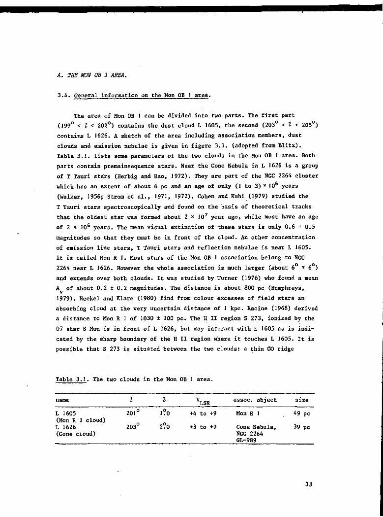
A. THE MON OB 1 AREA.

3.4. General information on the Mon OB 1 area.

The area of Mon OB 1 can be divided into two parts. The first part

(199° < I < 202°) contains the dust cloud L 1605, the second (203° < I < 205°)

contains L 1626. A sketch of the area including association members, dust

clouds and emission nebulae is given in figure 3.1. (adopted from Blitz).

Table 3.1. lists some parameters of the two clouds in the Mon OB 1 area. Both

parts contain premainsequence stars. Near the Cone Nebula in L 1626 is a group

of T Tauri stars (Herbig and Rao, 1972). They are part of the NGC 2264 cluster

which has an extent of about 6 pc and an age of only (1 to 3) * 106 years

(Walker, 1956; Strom et al., 1971, 1972). Cohen and Kuhi (1979) studied the

T Tauri stars spectroscopically and found on the basis of theoretical tracks

that the oldest star was formed about 2 * 107 year ago, while most have an age

of 2 x JO6 years. The mean visual extinction of these stars is only 0.6 ± 0.5

magnitudes so that they must be in front of the cloud. An other concentration

of emission line stars, T Tauri stars and reflection nebulae is near L 1605.

It is called Mon R 1. Most stars of the Mon OB 1 association belong to NGC

2264 near L 1626. However the whole association is much larger (about 6 * 6 )

and extends over both clouds. It was studied by Turner (1976) who found a mean

A of about 0.2 + 0.2 magnitudes. The distance is about 800 pc (Humphreys,

1979). Neckel and Klare (1980) find from colour excesses of field stars an

absorbing cloud at the very uncertain distance of 1 kpc. Racine (1968) derived

a distance to Mon R 1 of 1030 ± 100 pc. The H II region S 273, ionized by the

07 star S Mon is in front of L 1626, but may interact with L 1605 as is indi-

cated by the sharp boundary of the H II region where it touches L 1605. It is

possible that S 273 is situated between the two clouds: a thin CO ridge

Table 3.1. The two clouds in the Mon OB 1 area.

name LSRassoc. object size

L 1605 20F(Mon R 1 cloud)L 1626 203(Cone cloud)

1?

2?

0

0

+4

+3

to

to

+9

+9

Mon R 1

Cone Nebula,NGC 2264GL-989

49

39

pc

pc

33

2.0

0.0

i

2.0

4.0

-

X

X vX X

-xx

X

_

1 1

X

X

(1

\

<—>

^ .

x

/ffX

Monloop

„ * * x

\ \]

— — -

1

X

1

x ii/

/>i

cX- X

X "\

^ N G t

*s

i

z'j

j NGC

^ ; \ *\ v >̂

V l\ j

\ \>

„ / ^/ r/ •••i.

/ • • •

^ X *^ *s

?244iosette Nebuia

Xi

HJ626 ^

N

X

X

X

V

r05 ^Mon R1

XX

X

1 1

II

1

-

>

-

-

_

1

210.0 208.0 206.0 204.0 202.0 200D 1980

Figure S.I. Sketah of the area near the Mon OB 1 and 2 associations. Members

of Mon OB 1 are indiaated by a plus and members of Mon OB 2 by a

cross. Full drawn lines indicate dark clouds,, dashed lines emission

nebulae and dotted lines reflection nebulae. One degree corresponds

with 14 pa at the distance of Mon OB 1 and with 26 pa at the dis-

tance of Mon OB 2.

between the two clouds is partially in front of S 273. This and the almost

equal radial velocities of L J605 and L 1626 indicate that both clouds are at

about the same distance. The nature of a semicircular Ha emission structure

at the high longitude side of L 1626 is uncertain. It has an intensity mini-

mum at the position of L 1626, so it may be partly behind this cloud. Two pos-

sible triggers of recent star formation have been proposed. The first should

be at the center of Mon R 1 which has a semicircular shape (Kutner et al.,

1978), although no trace of any object is visible. The second is possibly an "

H I shell, centered at S 273 with a radius of 25 pc and an expansion velocity

of J5 km s-1. The suggestion is by Blitz (1978), but I find it rather poorly

Substantiated. The position of most recent star formation seems to be the in-

frared source GL-989 (Allen, 1972) near the Cone Nebula, close to an H20 maser

source (Genzel and Downes, 1977) at (I, b = 203.32, 2.06).

34

2.0

0.0

0.0 -

204. 0 202.0 200.0

Figure 3.2. a.

Contour map of peak antenna

temperature at 1667 MHz in the

Mon OB 1 area. Contourvalues

are 0.04, 0.06, 0.08, ... K.

The crosses indicate positions

where the satellite lines have

been observed.

Figure 3.2.b.

The same map , but from 1665

MHz observations.

204.0 202.0 200.0

3.5. OH observations of the Mon OB J area.

The area of the Mon OB 1 association has been observed in the following

way. First the area (198°1 < I < 205?6, -0?7 < b < 3?5) has been covered with

a wide grid of points, 0.42 apart. Then I covered the area around the positions

with positive detections with a narrower 0.3 grid. Contour maps of the peak

antenna temperature, T in the main lines are given in figure 3.2. These T

values result from Hamming weighted spectra with a resolution of 0.6 km s"1.

The highest ! is 0.16K near the Cone Nebula. No OH maser was detected in

this area with an upper limit of about 0.8 Jy.

Contour maps of the antenna temperature integrated over velocity,

I = ƒ T dV are shown in figure 3.3. The integral has been corrected as well

as possible for errors remaining after subtraction of a second order polynomi-

al. The error in I is about 0.05 K km s"1. Because the lines are rather weak,

the linewidth cannot be determined by fitting Gaussians. Instead I obtained

an "effective linewidth" AV = I/T.. At some positions the lines have two or

35

0.0 -

Figure 3.3. a.

Contour map of integrated line

intensity at 166? MHz of the

Man OB 1 area.

Contourvalues are 0.1, 0.2,

0.3, 0.4 K km s~2.

204.0 202.0 200.0

0.0 -

20U.0 202.0 200.0

Figure 3.3.b.

The same map at 1665 MHz.

three clearly recognized components with different velocities. Each of the

components has a linewidth of about 2 km s"1 and the effective linewidth will

be the weighted sum of the linewidths of the different components. For the two

clouds the mean values of AV are not very different: in L 1605 3.6 + 0.5 and

3.2 + 0.2 km s"1 at respectively 1667 and 1665 MHz and in L 1626 3.6 ± 0.3

km s"1 for both transitions. The linewidth does not vary significantly with T..A

Contour maps of the 1667 MHz antenna temperature at fixed velocities be-

tween +3 and +9 km s are shown in figure 3.4. L 1626 has OH emission between

+3 and +9 km s .At the lower velocities the emission is concentrated mainly

in the Cone Nebula region (203.2, +2.0). At velocities between +7 and +9 km s"1

the emission shifts over to higher longitudes (I = 204°). The velocity struc-

ture of this cloud is rather complex; it shows, especially near the Cone Nebula

more than one velocity component. This behaviour is in contrast with L 1605,

which has only one velocity component at each position. However this component-1 -1changes gradually in velocity from +4 km s at high to +8 km s at low

longitudes. This gradient is also visible in the lower resolution (2.6 km s"1)

36

2.0

0.0

2.0

0.0

2.0

0.0

2.0

0.0

3.0 KM/S --

"i 1-5.0 KM/S --

ö ' -

T r

On 14.0 KM/S

O

6.0 KM/S -

7.0 KM/S --

0

9.0 KM/S -

0

I I I 1 L_

8.0 KM/S -

O

204.0 202.0 200.0

204.0 202.0 200.0

Figure 3.4. Contourmaps of the 1667 MHz antenna temperature at constant veloc-

ities of the Mon ÓB 1 area. Contourvalues are 0.04, 0.06, 0.08

... K. Crosses are plaaed at reference positions for convenience

of the reader.

CO. observations by Blitz and can be explained by rotation in a direction op-

posite to galactic rotation. The magnitude of the gradient is 0.13 km s"1 pc"1

corresponding to a rotation period of 4.8 x ]Q7 years. The sense and the size

37

son. o

203.0

202.0

201.0 -

T 1 r

- 4

i i i i

1 1 . 0 9 . 0 7 .0 5 .0 3 .0 1.0fcm/s

204.0

203.0

202.0

201.0-

8=2.0

t i i

1 1 . 0 9 . 0 7 . 0 5 . 0 3 . 0 1 .0km/s

202.0

201.0

I200.0

199.0

B=0.8

Figure 3.5.

l-V diagrams at three latitudes

in the Mon OB 1 area. Contour

values are 0.033 0.05, 0.07,

11.0 9.0 7.0 5.0 3 - ° k m f e1 - 0

of the rotation are the same as that of the large molecular cloud in Orion

(Baud and Wouterloot, 1980, chapter 2) and in the Rosette Nebula cloud (Blitz,

1978). I will come back to this in chapter 8. The velocity structure can also

be determined from the longitude-velocity diagrams in figure 3.5. L 1626 has

three components at velocities +3, +5 and +8 km s"1. In addition to these

components there is, especially at b = 2?3, an indication of a velocity gra-

dient. The direction of this gradient is opposite to the one in L 1605. The

velocity gradient of L 1605 is clearly visible. The diagrams will be discussed

in more detail in the nesTt section.

38

3.6. Analysis of the observations of the Mon OB ] area.

3.6.1. Comparison of OH data with data from CO and other molecules.

3.6.1.1. L 1626.

The contour maps of peak and integrated antenna temperature at 1665 and

1667 MHz (figure 3.2. and 3.3.) show a number of features that I want to dis-

cuss. At 1667 MHz L 1624 appears to consist of two major fragments (see figure

3.2.a.), of which the one at 1 = 203.2 coincides with the extensively studied

cloud near the Cone Nebula L 1626 as a whole has an elongated structure like

many other molecular cloud complexes. At 1665 MHz the highest antenna temper-

ature is found between the two 1667 MHz peaks, probably because of statistical

variations; in the maps of integrated line intensity the remaining 1665 MHz

peak coincides with a 1667 MHz peak. In figure 3.6.a. I show the map of peak12C0 temperature as given by Blitz and in figure 3.6.b. the same map, but now

convolved to the OH beam. The outline of the OH cloud is generally the same as

that of the CO and the positions of maxima agree (in contrast with the situa-

tion near the Rosette Nebula, section 3.9.). In figure 3.6.b. there is no

second CO peak as in OH in figure 3.2.a. due to the convolution. Blitz' 13C0

map, which is rather incomplete, is quite similar to the 12C0 map. Compare now

the OH and CO velocity information. This is not easy because the CO observati-

ons by Blitz have a lower velocity resolution (2.6 km s"1). than the OH data

(0.6 km s"1'). L 1626 shows OH emission between +3 and +9 km s"1 with a maximum

between +5 and +7 km s"1, see figure 3.5. Higher resolution observations, e.g.13C0 (Crutcher et al., 1973) show the same picture. There is some structure in

the velocity distribution of the emission. The l-V diagrams in figure 3.5. at

b = 2.0 show two components. One at +5 km s and a second at +8 km s"1 which

is at a somewhat larger longitude. I do not think that there is a velocity

gradient at b = 2?0. At b = 2?3 there is again emission at +5 km s"1 with a

third component at +3 km s"1. The component at +8 km s"1 shows a shift from

+7 to +9 km s"1 at I = 204°. It is not clear whether this shift continues for

I - 203 • In other words: whether the very weak emission at +7 km s"1 is real

and related to this component or the +5 km s"1 emission is the continuation.

At • Z - 202 the emission is very weak and the velocity is between 5 and 7

km s-i. A similar effect was found by Blitz (1978) in some higher resolution

(angular and velocity) CO observations near the Cone Nebula: emission at +5

to +6 km s"1 at (203.20, +2.11) and at +7 to +8 km s"1 at higher and lower

39

Figure 2.6.a.

Contoumaps of the peak12

CO temperature (from

Blitz, 1978) of the Mon

OB 1 area. Contour values

are 1, 2, ... if.

206.0 2020 2000

Figure 3.6.b.

The same map, but con-

volved to the OH beam.

2040 202D 200.0

longitudes. He attributed this to an ionization effect by the 0 7 star S Mon.

The gas at +7 km s"1 near this star is ionized and the gas at +5 km s"1 re-

presented the backside of a collapsing molecular cloud. Starformation is

occurring in this region as the detection of an IR source and an H20 maser

source showed. Rickard et al. (1977) in H„CO and Lang and Willson (1980) in

NH, and in OH also observed the shift in velocity. Lang and Willson suggest

rotation as an explanation, but they mapped only a small part of the cloud.

On the basis of the present observations this explanation can be rejected. The13C0 data by Crutcher et al. (1978) confirm the OH result that the +7 km s"1

emission at I < 203 is. weak so probably the high 12C0 antenna temperatures in

this area are due to higher kinetic temperatures and lower densities than at

higher longitudes. Summarizing the previous discussion: the L 1626 cloud has

a main component which shifts from +5.5 km s~^ at I = 202 to +9 km s"1 at

I = 204°. Probably through an interaction with NGC 2264 the velocities change

around I = 203° toward +5 km s"1. The hypothesis from Blitz that this emission

is from the backside of a collapsing cloud is probably too simple because high

40

resolution observations show more fragments in this area. The difference in

resolution and in observed area between the OH and other data is too large to

develope a more accurate model.

Apparently star formation occurs in the middle of the cloud and this is

unusual. In Hon OB 2, in Ophiuchus and in Orion, star formation occurs at one

end of an elongated cloud. The sizes of these four complexes are comparable,

50 to 70 pc, with the exception of Ophiuchus, which has a size of about 25 pc.

However, in L 1626 the situation near NGC 2264 is probably a projection effect.

Because the OH and CO column densities are not very high near the Cone Nebula

the line of sight does not coincide with the long axis of an extended complex.

The situation is probably identical to that of the Cep OB 3 clouds, which com-

plex will appear similar to L 1626 when the Cep OB 3 complex is viewed in a

direction perpendicular to the galactic plane (see Sargent, 1977).

3.6.1.2, L 1605.

The four OH maps of this cloud in figure 3.2. and 3.3. agree quite well.

The differences shown, I think are insignificant. The general outline of the

cloud is the same as that of the CO cloud in figure 3.6, but some difference

occurs again in the area of starformation at 1 = 201.5 near the R association.

The CO emission has a clear maximum of about 3 K, but only weak emission is

seen in OH. Kutner et al. (1978) showed that near the R association, which

has the shape of a semi circle, the CO emission has a velocity of 0 km s"1,

whereas the rest of the L 1605 cloud near this position has a velocity of

about +5 km s"1. The shape of Mon R 1 was attributed to the initiation mecha-

nism of the starformation process, 106 years ago, that led to the appearence

of Mon R 1. The maximum in CO near Mon R 1 ia not visible in OH and 13C0, so

the density is probably small in this area. The 1^C0 was only observed in a

small area around 1 = 201.5 and its large-scale distribution is unknown. The

velocity channel maps of the i2C0 in general show the same gradient as the OH

maps, mentioned in section 3.5. At all positions in this cloud only one com-

ponent was detected in OH, except possibly at (200 , 1°) where there is weak

emission at +6 and +9 km s"1.

3.6.2. Physical parameters.

As discussed in chapter 1 of this thesis I follow two lines of analysis

succesively.

41

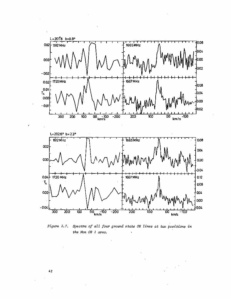
L=201°8 b=0.8°

0.02

0.00

-0.02

002

0.01TA

0.00

-0.01

H—I—I—I—I—h-d—I—I—I—I—[•1720 MHz

I I I I I "1Q.08

-0.04

-0.00

-Q02

I I, I I I I I I I I I I I I I I I I I I1667 MHz

-0.08

-0.04

.-0.00

-0.02

30.0 20D 1Q0 0.0, -10.0 -20.0km/s

20.0 10.0 0.0 , , -10.0km/s

L= 202.6° b=2.3°

0.02

0.00

0.04

0.00

-0.04

- 1612 MHz h 0.08

3Q0 20.0 1Q0 0.0 -10.0 -20.0km/s

20.0 10.0 00 , , -10.0km/s

Figure 3.7. Spectra of all four ground state OH lines at two positions inthe Mon OB 1 area. >

42

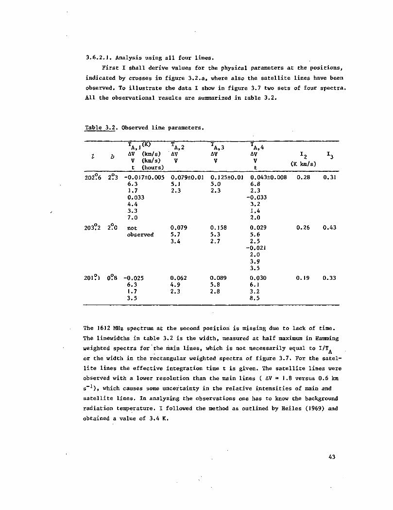
3.6.2.1. Analysis using all four lines.

First I shall derive values for the physical parameters at the positions,

indicated by crosses in figure 3.2.a, where also the satellite lines have been

observed. To illustrate the data I show in figure 3.7 two sets of four spectra.

All the observational results are summarized in table 3.2.

Table 3.2. Observed line parameters.

m /Vfc T ' T T

A , 1 A , 2 A , 3 A , 47 , AV ( k m / s ) AV AV AV I - I ,

V ( k m / s ) V V V , ™ . . ./i_ \ \K km/s)t (hours) t

202?6 2?3 -0.017±0.005 O.O79±O.O1 0.125±0.01 0.043+0.008 0.28 0.316.3 5.1 5.0 6.81.7 2.3 2.3 2.30.033 -0.0334.4 3.23.3 1.47.0 2.0

203?2 2?0 not 0.079 0.158 0.029 0.26 0.43observed 5.7 5.3 5.6

3.4 2.7 2.5-0.0212.03.93.5

201?l 0?8 -0.025 0.062 0.089 0.030 0.19 0.336.3 4.9 5.8 6.11.7 2.3 2.8 3.23.5 8.5

The 1612 MHz spectrum at the second position is missing due to lack of time.

The linewidths in table 3.2 is the width, measured at half maximum in Hamming

weighted spectra for the main lines, which is not necessarily equal to I/TA

or the width in the rectangular weighted spectra of figure 3.7. For the satel-

lite lines the effective integration time t is given. The satellite lines were

observed with a lower resolution than the main lines ( AV = 1.8 versus 0.6 km

s"1), which causes aome uncertainty in the relative intensities of main and

satellite lines.. In analyzing the observations one has to know the background

radiation temperature. I followed the method as outlined by Heiles (1969) and

obtained a value of 3.4 K.

43

At the first position of table 3.2 at 1612 MHz, there appears to be emis-

sion at 6.5 km s"1 and absorption at 3 km s"1 (see figure 3.7). In the 1720

MHz spectrum this seems to be reversed: absorption at 6.5 and emission at 4 km

s"1. Neither satellite line shows emission at 5 km^s"1, where the main lines

are strongest. A measurement error cannot be excluded, but I do not think it

very probable because the 1720 MHz spectrum at the second position 40 arc

minutes away looks very similar. It is remarkable that the main line velocity

is nearly the average of that of the emission and absorption features in the

satellite lines. A possible explanation is that in the two line wings the main

lines excitation temperatures are the same, but that those of the satellite

lines are different. Following the procedure outlined in chapter 1 I first

find the main line parameters (DT = 0 ) : T» = 0.6 ± 0.5, N-„ = (1.6 ± 1)+0 3

x 1015 cm"2, T = 3.7_" , K. Within the allowed optical depth interval I

find for T , > 0.6, T , and T . to be ̂ 3 K and ^ 5 K at the high-velocity

side and *»» 5 K and ^ 3 K at the low-velocity side of the line. For T, < 0.6,

T . and T . can no longer be determined accurately.£X}* GXf 4

There exist other cases where the excitation temperatures of the satel-

lite lines appear to be different at the two velocities on both sides of the

main lines. Crutcher (1977) found such differences ia the clouds in front of

3C 123 and W 40. This is possible if the gas emitting at these velocities has

different excitation conditions. According to the calculations of Guibert et

al. (1978) one will find T , > T , under normal circumstances. Howeverex, 4 ex,l

T , > T /is possible if the grain temperature is higher than normal. This

condition would be present only in a part of the cloud and needs systematic

motion within the cloud. This does only agree with a picture in which the

cloud is heated by the T Tauri stars and OB. stars which are in front of the

cloud if the highest velocities occur at the backside of the cloud. Crutcher

(1977) included the effect of radial velocity differences in his analysis and

obtained the opposite result for the relative magnitudes of the satellite line

excitation temperatures. This once again illustrates our lack of understanding

how OH is excited.

At the seeond position we have probably the same situation. Unfortunately

only the 1720 MHz line was observed. It shows emission at 5.6 km s"1 and ab-

sorption at 2 km s"1. The main line ratio points to a rather small optical

depth, T 3 < 1. The main line observations of Lang and Willson (1979) near this

position indicate a T, smaller than 0.2, but the uncertainty is rather large.

44

The third position shows a 1720 MHz line in emission and perhaps a 1612

MHz line in absorption (figure 3.7). From the main line ratio and assuming

DT = 0, I obtain T , = 1.2 + I, corresponding to a column density NQH =+0 5

(2.6 ± 2.0) x 1015 cm"2 and an excitation temperature T , = 3.6_n', K. If

the satellite line antenna temperatures are corrected for the lower velocity

resolution, many combinations of 1612 and 1720 MHz excitation temperatures are

possible, so I cannot say something more definite. Because the relative uncer-

tainties of the main lines at these 3 positions are large, it was not possible

to determine the eventual occurrence of DT ̂ 0. In the next subsection the

mean parameters of the clouds as a whole will be derived.

3.6.2.2. General analysis of the main line observations.

At positions where T. > 0.05 K the cloud averaged ratio of the peakA, J

antenna temperatures at 1667 and 1665 MHz is 1.45 (L 1626) and 1.36 (L 1605),

corresponding to an optical depth of T . = 1.1 ± 1 and 1.6 ± 1 respectively.

There is definitely a significant optical depth, although at some individual

positions the line ratio indicates T_ = 0. I will use the integrated antenna

temperatures I„ and I» and their ratio R^ = I3/I9 t o s e e whether there is a

difference in optical depth between the cores and the other parts of the

clouds. The advantage of the use of I over T. is that the number of usable

points is larger because the emission is weak and the lines are rather broad.

Table 3.3. Derived parameters for the two clouds in the Mon OB 1 area.

L_

0.

>

L_

0.

0.

>

*3

1605

10-0.

0.20

1626

10-0.

20-0.

0.30

19

19

29

N

15

12

13

13

4

1

1

1

1

1

«I

.67+0.

.73±0.

.77±0.

.26+0.

.52±0.

3

3

3

2

2

0

0

0

2

0

*3

.+1.2•4-0.4+] .0

" -0.2

,+0.9-0.1

•2-1.2„+0.9' -o. 7

T*T3

0.

0.

0.

1.

1.

7

7

1

1

1

Tex,3

3

3

4

3

3

.7

.7

.1

.6

.6

45

In table 3.3 the results are shown for the two clouds. N is the number of

points in the concerning I. interval. The optical depth in L 1605 in general

is low and does not show much variation over the cloud. It agrees within the

error with the value found from the ratio of the peak temperature. The uncer-

tainty in T_ is due to the uncertainty in F-. In the outer parts of L 1626 the

optical depth appears systematically lower than in the more central parts.

Notice that the second row of L 1626 (0.20 < I_ < 0.29) shows a very high

value, T, = 2.2; this has to be ascribed to the statistical uncertainty. The

mean value is about the same as that derived from the peak antenna temperature.

I now shall make an estimate of the mass of the clouds. If there is more

than one component, the integrated temperature gives a better value for the

total column density. Therefore I will use I, together with a mean value of

the optical depth (T* in table 3.3), where I have also considered the results

of the previous subsection and of the T line ratios. I adopt DT = 0 because

there are no indications otherwise. In this way I arrive at a mass of

(5.3 ± 1) x 104 M- for L 1605 and (5.2 ± ]) x JO" M. for L 1626. Not included

in the mass uncertainty is the (large) uncertainty in the OH abundance. The

total mass for the Mon OB 1 complex, (10.5 ± 2) * 10** M_ can be compared with

the value of Blitz, obtained from his CO observations. For CO the relevant

mass is the sum of "observed and halo mass", corrected for channel dilution

and non-LTE effects: (2.1 ± 1) x ]05 M_. This is observed within an area of19

7.2 square degrees. The observed OH cloud has an area of 5.9 square degrees.

The CO mass estimate, corrected to this size is (1.7 ± 0.7) * 105 Mfi, so the

masses from OH and CO just agree within the errors.

The masses, derived from OH and CO are for a filling factor F = 1; in

reality the estimates have to be multiplied by F and this factor is probably

< 1: OH observations by Riegel and Crutcher (1972) showed a peak temperature

of 0.24 K at (203?4, +2?0). Lang and Willsson (1979, 1980) mapped the core of

L 1626 near the Cone Nebula in OH with a 3.4 armin. beam. They found a cloud

fragment 9 arcmin. in size with a peak temperature of 0.87 K. This fragment

is probably embedded in the more extended cloud that I observed. CO observa-

tions by Crutcher et al. (1978) show that more fragments exist. Combining

these result I arrive at an estimate of about F = 0.4 in L 1626. There are in-

dications that fragments with sizes of typically 5 armin. are embedded also in

other parts of this cloud. Minn and Greenberg (1979) mapped two such fragments

in H.CO at about 0?5 distance from the Cone Nebula. It is difficult to detect

these fragments optically because L 1626 is largely behind the H II region

46

S 273. L 1605 was not studied as extensively as L 1626 and F cannot be deter-

mined. A more detailed discussion of the two different mass estimates will be

made after the results of the Mon OB 2 area have been discussed.

The mean density of both OH clouds is, dividing a mean value of N (for

F = 1) by an average width of the clouds, (80 ± 20) H_ molecules per cm3;

about the same value as Blitz found. However locally the density is much higher

if typical dimensions of CO fragments are used. According to the excitation

mechanism, outlined in chapter 1 (equation 1.1), using a mean excitation tem-

perature of OH, about 3.5 to 4 K and a kinetic temperature of about 10 K as

found from 12C0 observations one also finds that the density has to be low. It

would have been interesting to obtain T _ for the probably denser cloud thatex, j

Lang and Willson detected, but their measurements are not accurate enough to

determine optical depths. I do'expect a higher excitation temperature there,

corresponding to a higher density. This perhaps can be independently determined

by other means (e.g. H_C0 observations).

B. THE MON OB 2 AREA.

3.7. General information on the Mon OB 2 area.

The Mon OB 2 association is at a distance of 1500 pc (Humphreys, 1978).

Its 55 members of spectral type B 9 and earlier are found between I = 200 and

210° and b = -4° and +4°. Blitz (1978) discovered a large CO complex connected

with the association. The youngest subgroup of the Mon 0B 2 association is the

cluster NGC 2244 which is situated within the Rosette Nebula. An upper limit

for the age of NGC 2244 is 3 * 106 year. Recently Schneps et al. (1980) deter-

mined a kinematical age from CO measurements of small globules projected at

the Rosette Nebula of about 105year. Velocity gradients along elephant-trunk

globules were interpreted as stretching motions. This age agrees with a dyna-

mical age for the Rosette Nebula. The ages of other subgroups are 1.5 * 107

year and 5 x 106 year (Blitz, 1978). There is no clear indication how the for-

mation of the association developed in time, although most 0 and B stars are

to the north of the CO cloud complex. No young, low-mass stars (T Tauri stars)

are known, but they are expected to be detectable around m = 18 to 20. One

recent site of starformation is probably the IR source GL-961 (Cohen, 1973).

Blitz observed self-reversed CO at this position. There is no H„0 or OH maser

47

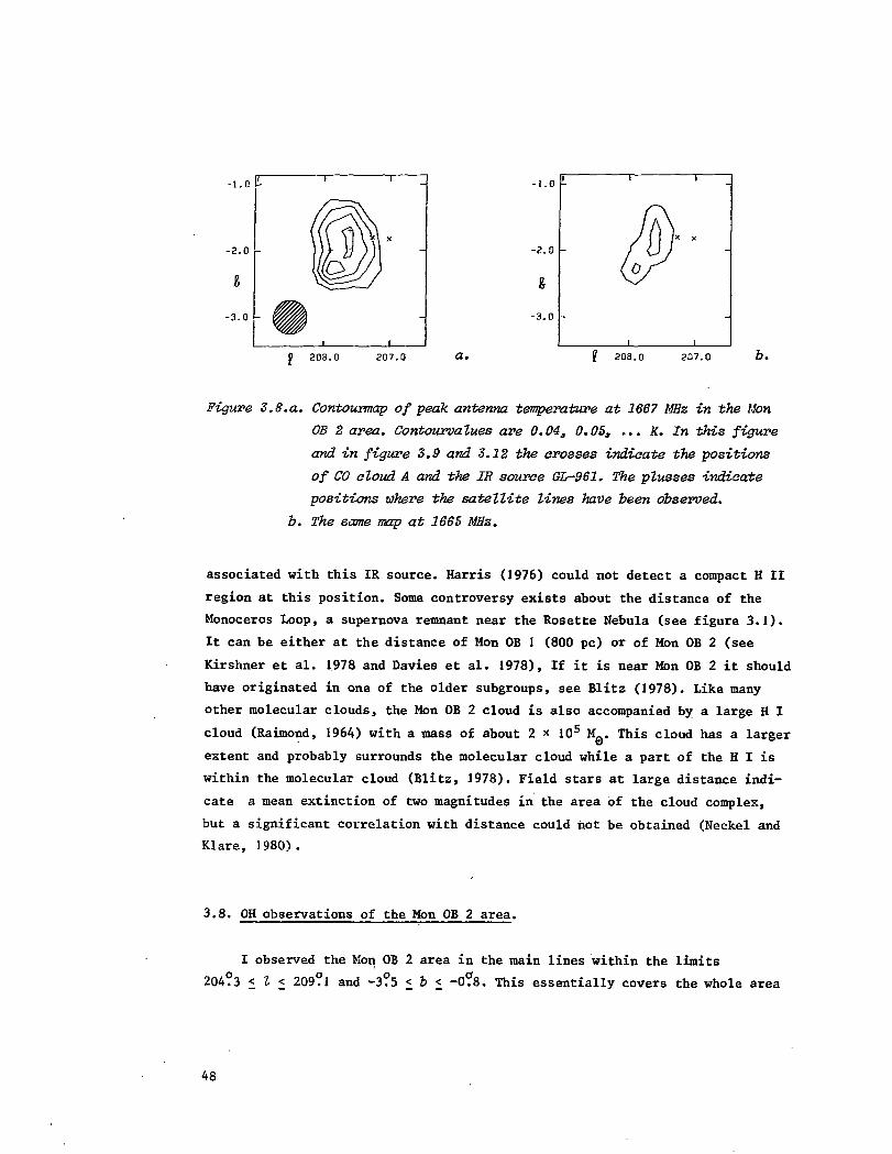
- 1 . 0 V- -1.0

-2.0

f,

-3.0

1 1

A(or

i

) ) • - -

-

208.0 207.0 l 208.0 207.0

Figuve 3.8.a. Contourmap of peak antenna temperature at 1667 MHz in the Mon

OB 2 area. Contourvalues are 0.04, 0.053 ... K. In this figuve

and in figure 3.9 and 3.12 the crosses indicate the positions

of CO cloud A and the IR source GL-961. The plusses indicate

positions where the satellite lines have been observed,

b. The same map at 1665 MHz.

associated with this IR source. Harris (1976) could not detect a compact H II

region at this position. Some controversy exists about the distance of the

Monoceros Loop, a supernova remnant near the Rosette Nebula (see figure 3.1).

It can be either at the distance of Mon OB 1 (800 pc) or of Mon OB 2 (see

Kirshner et al. 1978 and Davies et al. 1978), If it is near Mon OB 2 it should

have originated in one of the older subgroups, see Blitz (1978). Like many

other molecular clouds, the Mon OB 2 cloud is also accompanied by a large H I

cloud (Raimond, 1964) with a mass of about 2 * 105 M_. This cloud has a larger

extent and probably surrounds the molecular cloud while a part of the H I is

within the molecular cloud (Blitz, 1978). Field stars at large distance indi-

cate a mean extinction of two magnitudes in the area of the cloud complex,

but a significant correlation with distance could hot be obtained (Neckel and

Klare, 1980).

3.8. OH observations of the Mon OB 2 area.

I observed the Mon 0B 2 area in the main lines within the limits

204?3 < I < 209?l and -3?5 < b < -0?8. This essentially covers the whole area

48

-1.0 -

208.0 207.0 208.0 207.0

Figure 3.9.a. Contourmap of integrated line intensity at 1667 MHz in the Mon

OB 2 area. Contour values are O.l3 0.2, 0.3 K hn s .

b. The same map at 1665 MHz.

where CO was detected by Blitz (1978). Figures 3.8.a and b show contourmaps

of the peak antenna temperature in the 1667 and 1665 MHz lines (T. ..and T .)

respectively. The spectra have been hamming smoothed to a velocity resolution

of 0.6 km s"1. The highest value of T. , is 0.08 K. Figure 3.8 shows onlyA, i

small variations in T.; very probably larger variations exist, but the smear-

ing by our large beam has washed them out: the beamsize is 13 parsec. Figures

3.9.a and b show contourmaps of the integrated line intensity I = ƒ T dV. They

are not very different from figure 3.8. The linewidth is calculated as before

by dividing I by T. (max). A mean value at positions where I is larger than

0.10 K km s"1 is 4.1 + 0.7 km s"1 for the 1667 MHz line and 4.1 ± 0.5 km s"1

at 1665 MHz. There are no systematic variations of the linewidth over the

cloud.

Figure 3.10 shows contourmaps of the antenna temperature at 1667 MHz at

fixed velocities between +9 and +15 km s"1 with intervals of 1 km s*1. Easily

one distinguishes two separate cloud fragments. One fragment at a velocity

with respect to the local standard of rest.around 11 km s~V and a smaller one

at about 13 km s"1 projected against the first component. The resolution is

too poor to resolve different peaks within one component, e.g. the two peaks

at 11 km s"1 are not necessarily real. Another way to get insight into the

velocity structure of the cloud is by means of longitude-velocity (l-V) and

latitude-velocity (b-V) diagrams at 1667 MHz (figure 3.11). These again show

the two components even more clearly. The (b-V) diagram at I = 207?9 suggests

49

-1.0

-2.0

-3.0

-1.0

-2.0

-3.0

-1.0

-2.0 -

-3.0

9.0 KM/5

\ r

10.0 KM/S

12.0 KM/S

15.0 KM/S

I

13.0 KM/S

I I

11.0 KM/S

I L

14.0 KM/S

I

208.0 207.0 208.0 207.0

208.0 207.0

Figure 3.10. Contour maps of 1667 MHz antenna temperature at constant veloci-

ties in the lion OB 2 area. Contourvalues are 0,05, 0.04, 0.05,

... K. Crosses are placed as reference positions for the conve-

nience of the reader.

a weak velocity gradient within the main component in the sense that the

higher radial velocities occur at the higher latitudes. There is also some in-

dication that the radial velocity is somewhat higher at lower longitudes than

at the higher longitudes. The second component shows a shift from +13 km s"1

at J = 207?6 to +14 km s"1 at I = 207?9. However, the OH clouds do not show

a definite sign of rotation, as the CO clouds do (Blitz, 1978), probably be-

cause a significant part of the CO cloud which was not detected in OH (see

section 3.9.1).

50

-1.0 -

-1.0 -

Figure 3.11. An l-V and a b-V diagram in tlie Mon 0B 2 area. Contourvalues are

0.03, 0.04, 0.05, ... K.

3.9. Analysis.

3.9.1. Comparison with CO.

The dust cloud associated with the Rosette Nebula can only barely be

seen on Palomar Sky Survey prints. Because of the many foreground stars no va-

riation in extinction is visible within the cloud. The only other measurements

of the cloud are the CO map by Blitz and the H I measurements at 21 cm by

Raimond (1964). I will compare here OH and CO. In spite of the lack of detail

in the contourmap in figure 3.8, some conclusions may be drawn from the compa-

rison with the CO maps of Blitz. The part of the OH cloud at the highest galac-

tic longitudes appears to coincide very well with the CO cloud and with the

dust boundaries. Figure 3.12 shows the peak 12C0 temperature convolved to the

-1.0 -Figure 3.12.

Superposition of CO peak temperature,

convolved to the OH beam (contour-

values 1, 2, 3, ... K) and OH peak

antenna temperature (dashed, contour-

values 0.04, 0.05, 0.06, 0.07 K) in

the Mon OB 2 area.

208.0 2070

51

OH beam and superposed on the OH contours from figure 3.8.a. The crosses in

the figures 3.8, 3.9 and 3.12 indicate the positions of respectively CO cloud

A (as it was called by Blitz) and the infrared source GL-961. These correspond

to the most prominent features in the CO map. The rest of the CO emission can

be characterized by an extended cloud, called peak 6 by Blitz, with some small

high temperature regions at the edges. The 13C0 has the highest temperature in

the general area of cloud A and is extended in the direction of peak B. It is

not clear from the discussion by Blitz in which area he observed 13C0. In any

case the OH is only present in the extended low temperature peak B. In view of

the large difference in resolution the CO map of peak B and of the OH cloud

agree quite well in extent and in the position of the maxima. Blitz gives too

few details about the CO properties of peak B for a thorough comparison with

the OH properties. In CO it shows a lower temperature and a larger linewidth

than the rest of the cloud. Due to the lower velocity resolution in CO

(2.6 km s"1) Blitz could not have found the two components which I found in the

OH cloud (section 3.8), but the relatively large CO linewidth suggests that

these components are also present in the CO cloud. The absence of OH in the

cloud A part of the complex is real and asks for an explanation^ The first ex-

planation might be that the OH is not enough excited. The 13C0 antenna temper-

atures indicate that the density is considerable in this whole area, but actual

numbers are not known. Therefore it cannot be excluded that the mean density

in this area is critically smaller than in the rest of the cloud, and that OH

molecules are not enough excited. Such a lower mean density also could explain

the symmetry of the, Rosette Nebula, which has a rather low (electron) density

of around 20 cm~3. A second and third explanation for the absence of OH emis-

sion from cloud A follows from the fact that cloud A is situated relatively

close to the Rosette Nebula, which is seen projected over the outer parts of

cloud A. Because of the logrer density a part of the OH can be directly photo-

destructed by UV photons that escape the Nebula, or as pointed out by J. Black

(private communication), by collisions with C ions. These explanations will

have to be checked quantitatively. Better limits on the OH column density are

required; these can be obtained by observations with a larger telescope.

Required are also density estimates, e.g. through H-CO observations. Finally

a fourth explanation may be the following. The background radiation tempera-

ture was determined to be 3.4 K outside the Rosette Nebula. Continuum obser-

vations at 1400 MHz with a 10' beam.of the Rosette Nebula by Felli and

Churchwell (1972) show that a significant extra amount of continuum emission

52

-1 .0 -

- 3 . 0 -

Figure 3.13.

Contourmap of the Taurus complex asit would appear at the distance ofthe Rosette Nebula. Contour values0.04, 0.05, 0.06, ... K.

208.0 207.0

(a few K) is still present at the positions of cloud A and GL-961. If a signi-

ficant fraction of this emission comes from behind cloud A, the difference

(Tex 3 - TfiG) may be close to zero. This would mean that although OH can be

present, it is not observed. This can be verified by observations of other mo-

lecules.

Due to the large distance of the Rosette Nebula a lot of details are lost

in the OH map. To obtain an impression how many details are lost, compare

figure 3.13 and figure 5.2.a. They show the same object, the Taurus cloud com-

plex; figure 5.2 shows it observed at its real distance, J10 pc, and figure

3.13 at the distance of the Rosette Nebula, 1500 pc. At this absolute resolu-

tion the Rosette and the Taurus clouds look quite similar. Only further ob-

servations of the Rosette cloud with a much higher resolution (e.g. at Arecibo)

can decide whether they have really the same structure. This in spite of the

very different stellar populations. I will discuss this in more detail in

chapter 8.

"*.9.2. Physical parameters.

I will again follow the two lines of analysis, outlined in chapter 1.

Firstly 1 give an analysis of the observations at the positions where also the

satellite lines have been observed and secondly an analysis of the properties

of the whole cloud.

53

L=207.6°

i I i i i i i. ir) i i i i ï i1667 MHz

0.04

Q02

0.00

-Q02

0.06

0.04

0.02

0.00

-0.02

30.0 20JO 10.0km/sQ0 -100 20.0 10.0 0.0

Figure 3.14. Speatra of the fouv OH lines at one position in the Mon OB

2 aloud.

Satellite line observations were made at two positions with a high antenna

temperature at 1667 MHz. Figure 3.14 shows the spectra at one of those positi-

ons. The measured parameters of the lines at the two positions are listed in

table 3.4. The 1720 MHz line is missing at the second position due to lack of

observing time. At the first position the relatively high and equal antenna

temperatures of the satellite lines can only be obtained in the fitting proce-

dure if the optical depth T 3 is significant (> 1). The best solution is one

with DT = 0 K and T 3 = 1.5. If T 3 < 1.5 (and DT > 0.2 K), then the satellite

line predictions become too small (< 0.010 K). A small negative value of DT is

possible, but not necessary to explain the satellite line measurements. The

filling factor has no influence on the accuracy of the fit and I arrive at the

following result (for F= 1):

N0H

= 1.5*''!?, T = 3.5 K for all four lines,

5' 5-2^ X i o 1 5 cm~2' S u c n low, equal, excitation temperatures point to

a low density or to a low kinetic temperature (Guibert et al., 1978). At the

second position I have no 1720 MHz data, and a full solution of all parameters

cannot be found. The main line ratio points to t = 1.5 ± 0.8, T = 3.5 K

54

Table 3.4. Line parameters in the Mon OB 2 cloud.

TA;l ( K ) TA,2 TA,3V (km/s) V VAV (km/s) AV AVt (hours)

A, 4VAVt

(K km/s)

207?6 -1

2O7?9 -2?O

0.016+0.005 0.054±0.01 0.073±O.OJO 0.017+0.005 0.18 0.3810.74.620.0

0.0069.53.01J.5

11.54.4

0.04611.24.5

114.

0.06211.24.5

11.43.67.5

not observed 0.22 0.24

and N_„ = (5.6 ± 3) * 1015 cm"2. The 1612 MHz excitation temperature is betweenUn

3.5 K and 3.1 K and the predicted value of the 1720 MHz antenna temperature is

between 0.010 and 0.050 R.

Now I turn to the second line of analysis using the average properties of

the maj.ii line observations. Figure 3.15 shows a plot of T „ against T. , atA} £• A)j

nine positions in the cloud. Also drawn are lines for T_ = 0 (the lower line)

and T- = °° (DT = 0 is assumed). The r.m.s. noise in a single Hamming weighted

measurement is about 0.0J K. The mean yalue for the line intensity ratio is

1.50 ± 0.13. This corresponds to t. = 1 ± 0.5, which is in agreement with the

satellite line results. The derived T, is the value for the 11 km s"1 cloud

which has the highest antenna temperatures. To see whether there is any differ-

ence in optical depth between the center of the cloud and the outer parts and

0. 1

minia0.0 -

Figure 3.15.

Diagram of the peak antenna temper-

ature at 1665 MHz versus that at 1667

MHz in the Mon OB 2 area.

0.0 0.11667 MHZ TP

55

to incorporate the 13 km s~a cloud I have made a diagram similar to figure

3.15, but for the integrated line intensities. I find that for 0.10 < I < 0.20,

T , = 0.4+n"> and for I, > 0.20, x, = 0.7 _"_. This shows that the optical depth

is constant within the errors. Yet I use these values because I also consider

the earlier evidence of a higher T in the cloud center. I shall use the inte-

grated line intensity data to calculate column density and mass of the cloud.

A lower limit for the cloud mass is 2 x lO* M if T, = 0 and T _ = 10 K.

However for T , = 1, as derived above, the mass is higher: the average column

density in the cloud center is about (2.2 ± 1) x 1015 cm"2, only slightly

lower than the peak value at position (2O7?6, -l?7). The total mass of the

cloud is (2.3 ± 1) x 105 M-, where the errors are determined by the uncertain-ty

ty in optical depth. The mass of 2.3 * 10s H is distributed over two clouds,

with 60% in the +11 km s"1 cloud and 40% in the 13 km s"1 cloud. The mass can

be compared with the CO mass obtained by Blitz. I take only the sum of Blitz's

observed and 'halo1 mass: (2.1 + 0.7) * 105 MQ. The total area of the CO cloud

is 2.5 square degrees and that of the OH cloud is 2.0 square degrees. The

equivalent mass of the CO cloud is then reduced to (1.7 + 0.6) * 105 M a and

the agreement between OH and CO mass is quite good. However one has to keep in

mind that F can be smaller than I.I will return to these masses at the end of

this section. The mass estimate is valid for a filling factor F of 1.0, which

is uncertain (see at the end of the previous section the comparison with the

Taurus complex). However the CO observations with a beam of about 3 par sec do

not show much structure in his peak B. So if the cloud is fragmented it is on

scales less than about 5 pc (Jl arcminutes). The more detailed observations

of the lower density, (probable) higher temperature clouds by Blitz show frag-

ments 0.5 arcminutes in size and separated by about 10 arcminutes, so at least

in these parts of the complex F is < 1, although F < 0.1 is excluded. If this

is also valid for the OH cloud the most probable value is between 0.4 and 1.0.

A value of 2,2 x JO15 cm"2 for the mean column density in the center of

the OH cloud, an abundance of 1.1 * 10~7 (at T_ = 0.7) and a cloud thickness

of 24 pc (the width of the OH cloud at a level of 0.04 K) indicates a mean

density of 130 H_ molecules per cm3. Blitz gives 48-96 cm"3 over the whole

cloud. He obtained this value by dividing the mass by the surface area to the

power 1.5. If I so the same for OH I find 70 ± 30 cm"3. This low mean density

does not exclude the presence of many clumps with a higher density

56

(̂ 1000 cm"3) but I cannot detect these because of my poor angular resolution.

If the absence of OH in cloud A and near the IR source is not caused by the

higher continuum background temperature, an upper limit 3,'or the OH column

density in this area is 4 * 1013 cm"2 (I assumed T , = 10 K and T , = 0).

Then the total column density is < 7 x 1020 cm"2 which indicates a mean densi-

ty < 30 cm"3. The above adopted line of sight dimensions of 40 or 24 pc pro-

bably are upper limits, because observations of more local clouds (e.g. see

chapter 5) indicate that these kind of complexes can be rather flat, which

follows from the absence of many different auperposed velocity components. If

this flatness is considered the mean density in areas where is OH can be sig-

nificantly higher, perhaps up to 500 cm"3.

The kinetic temperature T.. is in most circumstances an upper limit for

the excitation temperature of OH (see chapter 1). One can estimate T R from

the CO observations of Blitz. In peak B he detected a peak antenna temp»-rature

for 12C0 of about 3 K, corresponding with a CO excitation temperature of 6 K.

Observations with better angular and velocity resolution in other parts of the

clouds show an increase in antenna temperature by a factor 3. Although in the

area of peak B this factor may be smaller due to the broader lines, an upper

limit for the CO excitation (and so kinetic) temperature is 12 K. The low mean

density, obtained with the high estimates of the cloud dimensions, together

with a kinetic temperature of 8 to 10 K gives, according to the simple excita-

tion mechanism, outlined in chapter 1 an OH excitation temperature around 4 K.

This agrees with the observational results if F = 0.4 and T_ < 0.5. But if the

cloud dimensions are smaller, the expected excitation temperatures will be

much higher than observed and again a better understanding of main lines ex-

citation of OH is needed.

One of the results of this section and of section 3.6 is the relatively

good agreement between masses derived from OH and from CO observation. Although

such a comparison is possible for only a few of the other clouds described in

this thesis, the difference is usually rather small. However, one has to keep

in mind that the mass, derived from OH is quite often only an upper limit: the

influence of the filling factor F has already been mentioned. The linewidth

can introduce errors because of the possible presence of two components at

different positions within the beam will cause a large apparent linewidth and

a too large mass. This will also happen in parts of the clouds where large

velocity gradients occur. To illustrate the effect of the linear resolution

I calculate the mass of the Taurus complex from the data in figure 3.13. Due

57

to the large absolute beamsize the apparent surface area is increased with

25%. With a mean value of T, = 0.7 for the whole cloud (derived from the ori-

ginal data), I obtain amass of 6.2 x 101* Mfl, which is a factor 4 too high. A

part of this increase will be caused by the fact that the relative increase

for low optical depth parts is larger than the decrease for the other parts of

the clouds. It should be noted that the increase in mass with a factor 4 is

equal to the decrease in peak antenna temperature. It is conceivable that

these effects are also present in the clouds described in this chapter, in

which case the cloud masses are overestimated by a considerable amount. Then

the masses derived from OH will be lower than the masses derived from CO by

Blitz and not higher, as the results by Solomon and Sanders (1980), who used

a smaller CO abundance, suggest. I shall resume this discussion in chapter 8

of this thesis.

3.10. Conclus ions.

In the Mon OB 1 area I mapped in OH two large, loosely connected molecu-

lar clouds each with a size of about 45 pc. Their extent in OH is nearly the

same as that in the CO maps by Blitz. The masses are 5.2 x 101* M for L 1626

and 5.3 x 101* Mfl for L 1605. The mean density of the cloud complex is

80 ± 20 cm"3. There, are some indications that the filling factor is about 0.4,

in which case the mass derived from OH is lower than that from CO. L 1605 has

a velocity gradient, suggestive of rotation with a period of 4.8 * 107 years.

The velocity structure of L 1626 is not as clear; it shows multiple components.

The satellite lines reveal that there are possibly excitation differences be-

tween the two velocity sides of the lines in the center of L 1626. One possi-

ble explanation is that one side of the cloud is locally heated.

A large molecular cloud in the area of Mon OB 2 was also mapped in the

main lines of OH. It shows the same extent in OH as the low temperature part

of the CO cloud, mapped by Blitz. The high temperature part of the CO cloud,

closest to the Rosette Nebula, could not be detected in OH, possibly because

of a lower OH abundance or of weaker OH excitation caused by a lower gas dens-

ity. A lower gas density will also explain why the Rosette Nebula is circular

although it borders on a molecular cloud. The average OH column density is

about 2 x 1015 cm"2. The total mass of the cloud detected in OH is (2.3 ± 1)

x 105 M , divided over two components with different velocities (+11 and

58

+13 km s"1). This mass estimate agrees with a value, independently obtained

from CO observations. The mean density of the cloud is 70 ± 30 H,, molecules

per cm3. This number is subject to all kinds of uncertainties but it suggests

the presence of high density clumps in the complex, embedded in a lower densi-

ty medium, as is the case in Taurus. To check this higher resolution OH obser-

vations are desirable. Such observations also have to be made of the areas of

cloud A and GL-961, to see if the mean density there is really much lower than

in the rest of the cloud. H-CO observations can indicate whether the increase

in continuum background emission plays some role in the decrease in OH antenna

temperature near cloud A.

References.

Allen, D.A., 1972, Astrophys. J. J_72, L 55.

Blitz, L., 1978, thesis. Columbia University.

Blitz, L., Thaddeus, P., 1980, Astrophys. J. 241, 676.

Cohen, ,M., 1973, Astrophys. J. 185, L 75.

Cohen, M., Kuhi, L.V., 1979, Astrophys. J. Supp. 4^, 743.

Crutcher, R.M., 1977, Astrophys. J. 216, 308.

Crutcher, R.M., Hartkopf, W.I., Giguere, P.T., 1978, Astrophys. J. 22^, 839.

Davies, R.D., Elliott, K.H., Goudis, C , Meaburn, J., Tebutt, N.J., Astron.

Astrophys. Supp. J}1_, 271.

Felli, M., Churchwell, E., 1972, Astron. Astrophys. Supp. _5, 369.

Genzel, R., Downes, D., 1977, Astron. Astrophys. Supp. ̂ 0 , 145.

Guibert, J., Elitzur, M., Nguyen-Q-Rieu, 1978, Astron. Astrophys. £6, 395.

Harris, S., 1976, Month. Not. RAS \Tk_, 601.

Herbig, G.H., Rao, N.K., 1972, Astrophys. J. VU_, 401.

Heiles, C , 1969, Astrophys. J. JS?, 123.

Humphreys, R.M., 1979, Astrophys. J. Supp. 38, 309.

Kirshner, R.P., Gull, T.R., Parker, R.A.R., 1978, Astron. Astrophys. Supp. 31,

261.

Kutner, M.L., Tucker, K.D., Dickman, R.L., 1978, Astrophys. J. 232, 724.

Lang, K.R., Willson, R.F., 1979, Astrophys. J. 227, 163.

Lang. K.R., Willson, R.F., 1980, Astrophys. J. 238, 867.

Minn, Y.K., Greenberg, J.M., 1979, preprint.

Neckel, Th., Klare, G., 1980, Astron. Astrophys. Supp. 42, 251.

59

Racine, R., 1968, Astron. J. J73, 2 3 3 .

Raimond, E., 1964, Bull. Astron. Inst. Neth. _lj*> 191.

Rickard, L.J., Palmer, P., Buhl, D., Zuckermann, B., 1977, Astrophys. J. _213_,

654.

Riegel, K.W., Crutcher, R.M., 1972, Astrophys. J. 172, L 107.

Schneps, M.H., Ho, P.T.P., Barrett, A.H., 1980, Astrophys. J. 240, 84.

Solomon, P.M., Sanders, D.B., 1980, in: Giant Molecular Clouds in the Galaxy,

ed. P.M. Solomon and M.G. Edmunds (Pergamon Press).

Strom, K.M., Strom, S.E., Yost, J., J97J, Astrophys. J. 165, 479.

Strom, S.E., Strom, K.M., Brooke, A.L., Bregman, J., Yost, J., 1972, Astrophys.

J. ]JJ_, 267.Turner, D.G., J976, Astrophys. J. 210, 65.

Walker, M.F., 1956, Astrophys. J. Suppl. 2, 365.

60

CHAPTER IV

OH OBSERVATIONS OF THE OPHIUCHUS COMPLEX

4.1. Abstract.

The molecular clouds near the Upper Scorpius association have been mapped

with the Dwingeloo telescope. The main lines were observed over an area of 48

square degrees and at four peak positions I also made satellite line observa-

tions. After a general introduction in section 4.2 I give in sections 4.3 and

4.4 a discussion of the method of observation and of the observational results.

In section 4.5 an analysis is made of the OH observations. The velocity struc-

ture of the cloud complex is discussed in section 4.6 and the relation of the

clouds with present and past starformation is discussed in section 4.7. In

4.8 I discuss the morphology of the whole region.

4.2. Introduction.

The complex of dark clouds near p Ophiuchi is one of the nearest regions

of recent starformation. The dark clouds in this area have been studied and

catalogued by Barnard (1927), Khavtassi (1960) and Lynds (1962). A sketch of

the area is given in figure 4.1.a, adopted from Khavtassi (see also

plate 3, which is from Barnard, 1927). The map by Lynds deviates in areas

where the extinction is light. Cross references of cloud names in figure 4.1.a

are listed in table 4.1. A complete overview of the whole region can also be

seen at plate 5 in the Atlas of the Northern Milky Way (Ross and Calvert,

1934). Some of the dark clouds have a very elongated structure. Often, and

also in this chapter, these features are referred to as "streamers", although

it remains to be proven that they really show or were formed through streaming

motions.

Many studies have been made of the dark clouds and of the objects associ-

ated with the dark clouds. The area is situated at the high latitude end of

Gould's Belt. Bok (1956) concludes from earlier work that the distance of the

61

Figure 4.1.a.

A sketch of the Ophiuchus area

from the atlas of dark clouds

by Khavtassi (1960). The hatched

areas are reflection nebulae* the

dashed lines indicate heavy obscura-

tion. The plusses are stars of the

Upper Scorpius association.

360.0 3S60 3520

Table 4.I. Cross references of the most important clouds in the Ophiuchus

area. Kh = Khavtassi (1960); L = Lynds (1962); B = Barnard (1927).

Kh 519 = L 1672 = B 229

Kh 527 = L 1675

Kh 536 = L 1676

Kh 538 = L 1680 + L 1687

Kh 547 = L 1681 + L 1709

Kh 563 = L 1712 + L 1729 + L 1761 + L 1763 = B 44 + B 238

Kh 567 = L 1739 + L 1740

Kh 569 = L 1717 + L 1719 + L 1752 + L 1757

L 1752 = B 43

Kh 584 = B 46

Kh 585 = B 45 = L 1744 + L 1755 + L 1765

Kh 596 = B 47 + B 51

B 4 6 + B 4 7 + B 5 1 = total of 12 Lynds clouds

Heiles' cloud 4 = L 1681

Streamer 1 = Kh 556 + Kh 567 + Kh 585

Streamer 2 = Kh 563

clouds is about 200 pc. The clouds are related with the Sco 0B 2 or Upper

Scorpius association. This is the youngest subgroup of the Scorpio Centaurus

assocition. Blaauw (1964) summarizes much work on this association. He derived

a distance of about 170 pc to Sco 0B 2. Garmany (1967) arrives at the same

62

result and I shall adopt this value throughout this chapter. The clouds are

often referred to as the p Ophiuchi clouds. This star actually consists of a

group of four stars surrounded by reflection nebulae (spectral types B2 IV,

B2 V, B5 V, B5 V) which are members of the association and is at a projected

distance of 1.2 (or 3.6 pc) from the center of the cloud. The cloud center is

closest (1 pc) to another association member, the B2 V star HD 147389 at

(352.85, 17.03). Cohen and Kuhi (1979) studied the T Tauri stars in this area.

Elias (1978) detected a number of possibly associated IR sources. Vrba (1977)

determined the direction of the magnetic field in the clouds by means of polar-

isation studies.

The radio continuum was studied at two scales. Falgarone et al. (1980)

made some high resolution radio maps of small H II regions near the core of

the molecular cloud, that are excited by some B-stars. Baart et al. (1980)

detected an extended region of radio continuum emission, probably related to

the upper Scorpius association. In a study of a part of Gould's Belt, Strauss

et al. (1978) observed this area in H I, but the dark clouds are at the edge of

the mapped area. Sancisi and Van Woerden (1970) discussed a region of H I emis-

sion with a velocity which is different from that of the other objects in the

same area. Myers et al. (1978) observed the self-absorbed H I in the area of

the dark clouds. The Cos-B satellite detected the Gamma-ray source CG 353 + 16

near the cloud complex (Bignami and Morfill, 1980).

Observations of molecules within the clouds have been made by Turner

(1973) and Encrenas et al. (1975). Myers et al. (1978) observed a variety of

molecules near the center of the cloud. Apart from a few OH observations by

Crutcher (1973) and the H_CO observations along the streamers by Heiles and

Katz (1976) all molecular observations concern a small area of about 0.8

square degrees. Baud made a first effort to study a larger area in an OH pilot

survey with a low sensitivity using the Dwingeloo telescope. Because of the

weakness of the lines, his search had little succes, but made it likely that

a deeper survey would be worthwhile. Subsequently I made the survey described

in this chapter.

4.3. The observations.

The Ophiuchus clouds and the Taurus complex (chapter 5) were observed in

the same way to make a comparison possible. The observations were made with

63

19.0

15.0-

11.0

XXXXXXXX) KXXXXX» < X X XXXXXXXXX? XXXXXXX KXXXXXXX

xxxxxxxxxxxxxxx.x>ix>d

XXXXXXXXxxxxxxXXXXXXXXXxxxxxxxxxxKXXXXXXXXXxxxxxxxxxXXXXXXXXxxxxxx

Figure 4.1.b.

The positions observed in OH

(crosses)3 divided over regions (a

to f) that are discussed separately.

360.0 356.0 ! 352.0

the 25 m radiotelescope in Dwingeloo during 3979 and 1980. The system temper-

ature of the helium cooled receiver was about 38 K. I made observations at a

grid of positions, 18 arcminutes apart, which is 60% of the HFBW. Each posi-

tion was observed during 30 minutes in a total power mode. Reference spectra

were taken at the north pole. The 256 channel autocorrelator was split into

two equal parts, each with a bandwidth of 625 kHz, the first one being used

at 1665 MHz and the second at 1667 MHz. This resulted in a resolution of

0.9 km s"1. The r.m.s. noise in each spectrum was about 0.02 K. The declina-

tion of Ophiuchus is so low that only 8 positions per day could be observed

and a fully sampled, unbiased survey was excluded. I therefore selected the

areas to be observed from Khavtassi's (1960) atlas of dark clouds. The posi-

tions observed are indicated in figure 4.1.b. The total area observed is 48

square degrees. Some of the positions which showed up as peaks in our OH

distribution were subsequently observed in the satellite lines at 1612 and

1720 MHz. These observations were made in the frequency switched mode with an

integration time of 4 hours (r.m.s. noise about 0.01 K).

4.4. The observational results.

The distribution of the peak antenna temperature is shown for the two

main lines in figure 4.2. One can distinguish two main areas of OH emission.

In the first area the p Ophiuchi cloud and the streamers that emerge from it.

In the second area the clouds around (358°, +19°), associated with L 1719,

64

19 .0 -

l -

19.0

'5.0

11.0-

'SJ

360.0 360.0 356.0 f 352.0b.

Figure 4.2.a. Contourmap of the peak antenna temperature at 1667 MHz. Contour-

values are 0.043 0.06, 0.08, 0.10, 0.14, ... X. Crosses indicate

positions where satellite lines have been measured.

b. The same map as 4.2.a, but at 1665 MHz.

LI 752 and L 1770 and embedded in the complex Kh 569. It is probable that the

complex is more extended below the Dwingeloo horizon, e.g. the clouds L 1672

and Kh 531 could not be observed. The most striking feature in the first area

is the strong peak of about 0.28 K at 1667 MHz near the center of the p Oph

cloud. This is by far the highest T in the whole region. In addition there

are a number of less intense peaks of about 0.10 K, all embedded in a back-

ground cloud of 0.05 K or less. At some places I observed this very low inten-

sity cloud incompletely, but judging from the optical appearance of the cloud

at the POSS prints and from incidental observations outside the mapped area,

it is unlikely that the low intensity cloud extends much beyond the limits in-

dicated in figure A.2. Of the two streamers, the upper one (streamer 1, which

is divided into three parts, Kh 585, 567 and 556, see figure 4.1.a) was de-

tected over its full length, whereas the lower one (streamer 2, consisting of

Kh 563 and a more fragmented part of longitudes larger than 358 ) was only

detected at its very beginning and further "downstream" at a few positions

and rather marginally. The second area, containing the Kh 569 complex, is

optically less visible at the POSS prints. This implies more foreground stars

or less extinction. However it showed up in the OH lines over quite a large

area as can be seen in figure 4.2.

65

19.0- 19. D -

15.0 -

11.0- 11.0-

360.0 356.0 t 353.0

a.360.0 356.0

Figure 4.3.a. Contour map of the -integrated line intensity at 1667 MHz. Con-

tourvalues are 0.10, 0.15, 0.20, ... K ten s~ .

b. The same map, but at 166S MHz.

Figure 4.3 shows the antenna temperature, integrated over 7 km s"1 cen-

tered at the velocity with the highest T.. There are a few differences in

these figures when compared with figure 4.2. Some of the low level peaks in

figure 4.3, e.g. those near (357.5, +16 ), which cannot be seen in figure

4.2.a are probably caused by remaining baseline inaccuracies in the spectra.

Streamer 1 is rather weak in figure 4.3.a because the linewidths within this

streamer are somewhat smaller than in the rest of the clouds.

The Ophiuchus complex contains, just like the Taurus clouds, no maser

sources stronger than 0.4 Jy.

4.5. Analysis. s

In this section I shall first analyse the observations at the positions

where all four 18 cm OH lines have been measured. Second I shall analyse the

main line observations in several parts of the total cloud complex.

66

U3S276 b- ia6"

002

0.00

• 1720MHz

1 I 1 I 1 I I I 1 I .1 I I I I I 1 I I I

0.08

OOt

000

012

ooe

OOt

000

Q08

004

000

. 1667 MHz

200 100 00 km/s -100 200 100 00 km/s -10.0

L=3539° b=15.7°

0.02 -

000 •

I I I I I I I I I I I I I I I I I I I II I I I I I I I I I I I I

001

- 000

-008

-004

-D.00

200 100k m , s

200 100 0 0 km/s -1Q0

Figure 4.4. Spectra of the four lines at tuo selected positions.

67

4.5.1. Analysis of satellite line observations.

I have made satellite line observations at four positions in the cloud

complex indicated in fig. 4.2a. The spectra at two positions are shown in

figure 4.4. Table 4.2 gives the observed values of the line parameters. The

uncertainties in the values of T. . are about 0.015 K. In all cases the 1612A,i

MHz line is very weak and the signal to noise ratio is about 1. I estimated the

excess (galactic) background temperature from the maps of Seeger et al. (1965)

and obtained a value of about 0.9 K. Together with the cosmic background I

find T_- = 3.6 K. The first position in table 4.2 is somewhat outside the

center of the cloud. Following the method of analysis outlined in chapter 1,

I find T_ = 1.0 ± 0.6 and DT = 0. The uncertainties in the measurements allow

DT to be positive, but if DT > 0.5 K, the predicted 1720 MHz antenna temper-

ature becomes too small. For DT = 0 the column density NQ = (1.5 ± 1.0) x

1015 cm"2. The largest possible value of DT (0.5 K) reduces this number by a

factor five. The filling factor F, assumed to be 1.0, may be smaller if

T, = 1.6, at the high side of the permitted interval. The limits for DT then

Table 4.2. Values of the observed parameters of the four ground state lines

at selected positions.

1. 352.7 16.6 -0.022 0.097 0.163 0.080 0.167 0.313

2. 353.9 15.7 -0.019 0.106 0.092 0.064 0.178 0.203

TA.lV

AV

-0.0223 . 21.5

-0.0194 . 20 .5

0.021.41.2

-0.0162 .81.0

TA, 2V

AV

0.0973 . 61.7

0.1064.11.5

0.0400 . 82.5

0.0612 .61.8

TA,3V

AV

0.1634.01.8

0.0924 . 31.9

0.0911.41.7

0.0843 . 01.5

TA,4V

AV

0.0803 . 61.7

0.0644 . 21.5

0.0321.01.5

0.0682.51.9

3. 356.3 19.3 0.02 0.040 0.091 0.032 0.126 0.190

4. 358.1 15.4 -0.016 0.061 0.084 0.068 0.073 0.081

68

are the same (DT < 0.5 K) but the associated reduction in N is smaller.Uli

Turner (1973) observed a point at a nearby position which he called

4C (353.05, +16.67); it is at the center of the p Oph cloud. His result was

T. , < 0.01 K, T. _ = 0.45 K, T. = 0.80 K and T, . = 0.2 K. This combina-A,l ' A,2 ' A,3 A,4

tion of satellite line temperatures is only possible if T_ is smaller than

0.8 and with a preference of a value near T , = 0 due to the main line ratio.

If the optical depth or the filling factor become too small (T, < 0.1;

F < 0.5) or if DT > 0.1, then T _ will be larger than 20 K which I consider

improbable. A negative DT of a few times 0.1 K is definitely possible. At this

position the value of T . cannot be determined with certainty. It is larger

than ̂ 8 K or smaller than -5 K. Comparison of Turners results at position 4C

with those at my first position indicates that the excitation conditions in

the center of the P Oph cloud appear to be different from those in the sur-

rounding part of the cloud (see table 4.3). The optical depth in the cloud

center appears to be smaller than at a position outside the center. This will

be discussed later in more detail.

At the second position in table 4.2 I have made two different observati-

ons of the two main lines. In one case T. _ is marginally larger than T. _,

in the other T „ = T . This indicates a rather large optical depth T,.

Requiring also a fit with the satellite lines for DT = 0 I arrive at T_ =

2 ± 1, N n = (3 ± 1) x 1015 cm"2; T = 3.5 K and T = 4.2 K, which are

normal values for other molecular clouds discussed in this thesis. An upper

limit on DT is 1.0 K, in which case a larger interval in T .is possible.

The filling factor remains undetermined.

The third position is in one of the condensations of the Kh 569 complex.

The main lines point toward a low optical depth T». However, if x3 < 0.8 the

1720 MHz line is predicted to be much weaker than observed. The most probable

value is T = 1 + 0.5, which means N = (1.5 ± 0.5) x 1015 cm"2. T and•J Uxl 63£y J

T . are nearly the same as at the second position, 3.5 and 4.0 K. DT has

to be zero or very small because otherwise the 1720 MHz line predictions

become too low. The actual value of the filling factor cannot be found be-

cause it has only little influence on the predicted line strengths. Also

optically it cannot be estimated because of the poor visibility of the Kh 569

complex on the FOSS prints.

The last and fourth position is within the Kh 585 part of streamer 1.

The optical depth is somewhat larger than at the previous position, t. *

1.5 ± 1, which gives N = (2.0 ± 1) x 1015 cm"2. Just as at the third

69

Table 4.3. Derived parameters.

1.

AC*.

2.

3.

4.

0

1

T3

.0±0

,8±0

2±1

l±0

.5±1

.6

.2

.5

Tex, 3

3.9

5.5

3.7

3.8

3.7

N0Hxl0l*

15±10

15

30±10

15+0.5

20+10

ex, I

3.3±0.3

3.6

3.5

3.5

3.3

Tex,4

6±2

>5

4.2

4.0

4.4

DT

<0.5

-0.2

<1.0

0

<0.4

From an observation by Turner (1973).

position a very small T_ is not possible and DT has to be smaller than 0.4 K.

T , and T , are 3.3 and 4.4 K. Because the streamer has optically nearlyex,1 ex,4

the same size as the beam (0.5), the filling factor probably is somewhat

smaller than one, but the actual value cannot be determined. A summary of

the results of this subsection is given in table 4.3.

4.5.2. Analysis of main line observations.

I divide the observed area into 6 regions (indicated in figure 4.1.b)

which will be treated separately.

a. The area around HD 147889.

b. The area around the beginning of streamer 2.

c. The rest of streamer 2.

d. The Kh 585 part of streamer 1.

e. The rest of streamer I.

f. The Kh 569 region.

The main results of the analysis of the observations are displayed in table

4.4. The optical depth was estimated by plotting T. 2 against T. _ for all

positions within one region. The same was done for I» and I_. Because in most

of the regions the lines are weak, I could not derive the optical depth for

individual positions, and only an estimate of the mean value of a whole re-

gion is given. The linewidths were determined by dividing I» by T. and I_

by T. _. The spread in AV within each region is a few times 0.1 km s"1. To

illustrate the effect of the incorporation of the line ratio I mention also

70

Table 4 .4 . Mean OH parameters in d i f ferent pa r t s of the complex.

region I b T_ AV T N„IT . N . n M . M_~_ 3 ex, 3 OH.min OH,max nun max

a

b

c

d

e

f

353°

354°

357°

358°

355°

357°

17°

15?5

14°

15?5

16°

20°

°-8-o'-0

-

i /+2K4-l

o+o

i.2

.6

.5

.3

.5

.5

.5

1.7

1.9

2.0

2.0

1.7

2.1

2.5

4

3

3

3

3

>3

'5-.;

.8

.8

-

.9

.8

.9

. 2.3

0.7

1.0

0.7

0.7

0.8

1.1

15 101*1 260 5300

17

25

-

9.2

26

120

150

150

230

500

2800

2100

6500

column densities and masses which are obtained if I assume that f_ = 0, listed

in table 4.4 as Nrt,T . and M . . However 1 do not consider these to be rea-OH.min mxn

listic numbers. I now discuss the regions in more detail.

Region a. This region contains the most studied part of the cloud complex. A

comparison of the OH map with the map of H I column densities derived from

H I selfabsorption by Myers et al. (1978) learns that OH was detected at po-

sitions where N > 1 x I020 cm"2. In a plot of T _ versus T _ of all posi-

tions in region a the line ratio at the three positions of highest T ap-A, J

peared to be higher than in the rest of this region. This points to a lower

optical depth in the center of the cloud (x. = 0) than outside the center

(T„ - 1). In the latter area the line ratio is constant within the errors.

Earlier observations of OH indicate an optical depth in the very central regi-

on of the p Oph cloud between 0 (Heiles, 1969), 0.16 (Turner, 1973) and 0.4

(Myers et al., 1978). These three values are not very accurate and equal

within the errors. It is easy to calculate a lower limit for the OH column

density by assuming an optically thin line and a high excitation temperature

in the whole ;loud such as Myers et al. did. In the present case this will

not result in difficulties. For this purpose I shall assume an excitation

temperature of 10 X. Then column densities range between 4.5 * 1013 cm"2 in

the outer parts of the cloud and 2.3•* 10*** cm"2 in the center. If the appa-

rent optical depths are taken into account and•incorporated (low in the center

and higher outside the center), a problem arises. The OH column density in

71

the cloud center will be lower than in the outer parts of the cloud. This

seems to be somewhat unlikely; because there are no heavy stars in this area,

photo dissociation cannot be more important in the center than in the rest of

the cloud and I cannot see a reason why the chemistry in this area will be

different from other clouds where this effect is not seen. The only way to ob-

tain a columndensity which is not decreasing toward the center of the cloud is

by assuming in the center of the cloud a slightly negative DT (about -0.2 K)

which means that T. is higher (T_ = 0.8) there than apparently observed, and

which is allowed by the satellite line data (section 4.5.1). This solution is

indicated in table 4.4 where the upper line is for the central positions and

the lower line for the rest of this region. Bujarrabal and Nguyen-Q-Rieu

(1980) showed that this situation (DT < 0) is possible if a cloud collapses

with a velocity between 0.9 and 1.2 km s"1. The necessary infrared radiation

probably is present in this part of the cloud. Myers et al. (1978) showed that

the linewidth of different molecular species decreases toward tue cloud center,

which could be explained by contraction. The (minimum) mass for T. = 0 in

region a is about 260 M_ and the mass for T_ = 0.8 is 5300 ML. The latter va-

lue must be considered as an upper limit due to the filling factor. If the

results of Myers et al. from 13C0 and from extinction are extrapolated to the

extent of the OH cloud in region a, I obtain a mass of about 2600 M_, which

agrees with the OH results if F = 0.5 and T, is high.

Region b. Region b is at a distance of about 1.3 (or 3.9 pc) degrees from the

P Oph cloud center and forms the beginning of streamer 2 (see figure 4.1). It

is not clear whether this streamer is related to the fragments in region a

which are directed towards region b and can be seen in H„CO (Myers et al.,

1978). The question of the origin of the streamers will be discussed in sec-

tion 4.8. Although the lines are weak (T. < 0.10 K), the optical depth in

this area appears to be somewhat larger than in region a. The measured antenna

temperatures are scattered around T_ = 1.4, but the uncertainty is rather

large. This estimate agrees with the estimate at position 2 in subsection

4.5.1. The mass in this region is between 120 and 2800 M_ for resp. T_ = 0.0

and T- = I.4.

Region a. Photographically streamer 2 has a very clumpy structure (see Barnard,

1927), apart from a region of about 2° in length, east of region b, I find

this back in the OH observations. The lines are very weak, also close to the

head of the streamer, near region b. There are only a few scattered positions

(0.1 to 0.7 square degrees in size) with detections of more than 0.04 K. This

72

can only partly be due to the small width of the streamer (0?6). Therefore I

cannot derive conclusions about the optical depth. Because in other regions,

e.g. Taurus, the optical depth mostly is lower in areas where the lines are

weak, I will assume T = 0. In this case the mass is 150 M , divided over 12

clouds between 5 and 45 K&. These values are very uncertain.

Region d. This is the area of streamer 1, called Kh 585, or B 45. In the OH

maps this cloud is stronger than streamer 2 (region c). The optical depth is

somewhat smaller than in region b. The observed linewidth is about 1.7 km s"1,

which is smaller (although not very significantly) than in other parts of this

cloud complex. The mass within this part of the streamer is probably between

150 and 2J00 M 0 for respectively T = 0 and t, = 0.6.

Region e. This is the part of streamer 1, between the end in region d and the

head in region a. Region e contains two dark clouds, Kh 556 and Kh 567. Kh 567

is a relatively small cloud and its OH lines are weaker than in Kh 556. There-

fore I have taken the two together. The optical depth in this region is compa-

rable to that in region b, but a very accurate number cannot be given. The

mean value of T„ is rather high and because the extent of region e is large,

the upper limit of the mass within this region is also high, 6500 Mo. The

lower limit is about 230 Mfl, 60% of which will be within Kh 556. I consider

the value of 6500 Mfl as too high, especially if this area is compared at photo-

graphs with region a and region d.

Region f. This region, that coincides with Kh 569, is probably separate from

the p Oph clouds (see section 4.6). The OH emission can be characterized by a

low optical depth and a large linewidth. Then the molecular mass is about

500 Mfl. (Using the highest value for x~, that is still acceptable, I obtain

6100 M 0 ) . The masses of the individual clouds are between 100 and

2000 M0.

Other, smaller regions beside the regions a to f are a few smaller iso-

lated low temperature clouds, especially L 1782 and 1796 between the regions

d and f and near region a. Their total mass is less than 100 M_ is T» = 0;

individual masses range from 7 to 20 M_.

In three cases in table 4.4 the derived optical depths are quite compa-

rable to the corresponding values in table 4.3. Those in table 4.4 are some-

what (except at position 3, where a larger difference exists) smaller, but

since these represent average values in the region and those in table 4.3

peak values, the difference is explainable. The fact that the average ratios

of the main lines and, at individual positions, the strength of all four lines

73

is explained by DT = 0 K and a significant value of T_ is reassuring and adds

some credibility to our conclusions. The masses in columns 10 and 11 of table

4.4 are lower and upper limits obtained for T_ = 0 and for T~, as derived. In

the lower limit the streamers contain more mass than the main region, whereas

in the other cases it is more equally divided over both parts.

A major problem in the interpretation is the filling factor F. At POSS

prints the whole region is characterized by structures with a width of about

0.5, the same as the size of the beam. If this causes F to be, say 0.5, the

lower limits are unaffected, but the upper limits of N_u per beam area de-

crease with a factor 2. Because the abundances were derived for F = 1, the

effect on the mass is uncertain. The total mass of the Ophiuchus complex

(region a to e) is 1.6 * 101* M , which is close to the mass of Complex A in

Taurus. However I have Indicated that the mass in region e, which would con-

tain an important fraction of the mass, probably is overestimated. I conclude

that the mass of the Ophiuchus complex is somewhat lower than of the complex

in Taurus, but since I have not made such uncertain corrections in other

complexes in this thesis, I shall adopt as the derived mass, (1.6 ± 0.6) x

lO4 MQ. The mass of the Ophiuchus complex is thus comparable with those of

other complexes (see chapter 8), but the differences with respect to the

other complexes (except Taurus, see chapter 5) seems to be. the very fragmented

nature of the Ophiuchus complex. As discussed in chapter 8, it is not at all

certain that this difference is real. Because the streamers are very narrow,

the Ophiuchus complex would have been undetected in OH at the distance of

Mon OB 2 where the Taurus clouds still are detectable (see chapter 3). It is

discussed in chapter 5 that in Taurus the dustlanes are less pronounced in

CO than in OH. It will be interesting to compare future CO measurements with

the present OH measurements.

In the different regions a mean density was derived by dividing the total

column density by the smallest dimension as seen on the sky. The results run

from about n.. =100 cm"3 for the regions c and f, via ny - 450 cm"3 for d

toward nu = 650 cm"3 for the regions a, b and e. The excitation mechanism2

of OH (Guibert et al. 1978 and chapter 1) requires a very low kinetic temper-

ature (lower than 5 K) to explain the derived excitation temperatures of

about 3.8 K if these densities are adopted. Such low kinetic temperatures can

be checked by CO observations. The mean density within the whole complex is

apparently larger than for other complexes at larger distance (see chapter 3)

where it is about 100 cm~3 or lower. This can be caused by not resolved

74

structures within the more distant clouds.

19.

15.0

11.0

0.0 KM/S

H 1-

I I " 1 1 i

1.0 KM/5

19.0

15.0

11.0

19.0

15.0

2.G KH/5

11.0 KH/S

11.0 i i i

3.0 HM/5

5.0 KH/S

I 1 1

360.0 356.0 35^.0 360.0 356.0 352.0

Figure 4.5. Contourmaps of T „ at fixed velocities between 0 and +5 km s

Contourvalues are the same as in figure 4.2.

-1

75

359.0 -

Figure 4.6.

Longitude-velocity diagram along streamer 1 at

1667 MHz. Contoupvalues ave the same as in

figure 4.2.

4.6. The velocity structure.

The velocity structure of the cloud complex can be determined from

figure 4.5, which shows the distribution of the emission in £ and i> at fixed

velocities between 0 and +5 km s"1. The following results can be obtained from

this figure: the emission of the center of the P Ophiuchi cloud is at

+4 km s"1. Streamer 1 has a constant velocity of about +3 km s"1. Some emis-

sion from Rh 567 is at +2 km s"1 and the positions where streamer 2 is detec-

ted are at +4 or +5 km s"1. Kh 569 is visible at +1 to +3 km s"1.

Figure 4.6 shows an l-V diagram along streamer 1 and through the center

of the cloud. This diagram is composed of a number of l-V diagrams put in

series with b between +15?1 near I = 360° and +16?9 near I = 352° and of

different longitude intervals. It shows that over a length of 5° the radial

velocity is constant. Only near the center of the cloud the velocity is

different.

Heiles and Katz (1976) observed H-CO with an 11 arcmin. beam at 37 posi-

tions along the streamers. In H_CO streamer 2 is detected at more positions

than in OH, probably because of their smaller beam. Their results concerning

the velocities are equal to those in figure 4.5: streamer 1 is at +3 km s"1

and streamer 2 is at about 4.5 km s""1, except at 2 positions, where it shows

76

emission at +2 km s"1.

Myers et al. (1978) showed that the molecular cloud in the area around

(353 , +16 ) has the same velocity as the neutral hydrogen which is seen in

selfabsorption. They showed also that there is a velocity gradient from

+5 km s"1 to +3 km s"1 through the center of the cloud about perpendicular to

the direction of the streamers, and that the H I emission is at about the

same velocity as the selfabsorption. The velocities of OH emission in region

a agree with the H I results by Myers et al. Because the OH emission is de-

tected at rather scattered positions it is difficult to determine a large-

scale velocity pattern from these results. Therefore I have extended the H I

data used by Myers et al. by using the Berkeley Survey (Heiles and Habing,

1974). The peak velocity of the H I was found by fitting a parabola through

the profiles where self absorbed parts were omitted. Although the uncertainty

in the resulting H I velocity is due to the asymmetric profiles rather large,

the difference with respect to the molecular velocity is zero within the

errors; this is true also for the velocities of the Kh 569 complex. The H I

velocity shows a gradient from +4 km s"1 near streamer 2 to +1 km s~J between

Kh 567 and Kh 569. At higher latitudes toward Kh 569 the velocities become

higher again. This is one reason why I think that Kh 569 is not directly

related to the other clouds, although the distance is not very different. The

situation may be similar to that of L 1605 and L 1626 near Mon OB 1 (see

chapter 3)• I see at this moment no explanation for the direction and the

size of the velocity gradient in this area. Vrba (1977) calculated the age of

the streamers by relating the difference in velocity of streamer and p Oph

cloud center to the distance between the two. However the result is doubtful

because Vrba used a wrong value for the velocity of p Oph cloud center (2.9

instead of 4.0 km s"1, probably caused by an unrecognized CO selfabsorption).

The observed linewidth within the molecular complex varies between

1.7 km s"1 in the p Oph cloud center and in B 45 to 2.5 km s"1 within the

Kh 569 complex. In the other parts it is about 2.0 km s~*. Because the reso-

lution was 1.1 km s"1, the true linewidths are between 1.3 and 2.2 km s"1.

The small linewidth within B 45 points towards little internal motions.

Myers et al. (1978) explain the smaller linewidth in the p Oph cloud center

to a retarded free fall. I also found a somewhat smaller linewidth in the

central area which agrees reasonably well with Myers1 et al. value at the

same radii.

77

26.0 -

22.0 -

1B.0 -

Hl.O -

10.D U359.0 355.0 351.0 3117.0 343.0

Figure 4.7. The positions of bright (&) and fainter (+) members of the Upper

Soorpi us association and of T TauH stars (x) with respect to the

molecular clouds.

4.7. Stars and starformation.

The Ophiuchus molecular cloud complex is connected with the Sco OB 2 (or

Upper Scorpius) association. This is a subgroup of the Sco Cen association

(Blaauw, 1964). It has a kinematical age of about 5 x 106 year and a photo-

metric age of about (6 ± 2) x ]06 year. The mean radial velocity of the stars

is 5 + 8 km s"1, nearly the same as that of the molecular cloud. In figure

4.7 I show the distribution of members of the association, with respect to

the molecular clouds; I owe the information on the stars to Mr. T. de Zeeuw.

78

The streamers all point away from the direction towards the association. Around

(350?5, +22?4) is the mean position of the origin of the association as it was

traced back from proper motions by Blaauw (1978). Blaauw mentions the possibi-

lity that there have been more than one center of starformation b-̂ c the precise

relation of these centers to the present outline of the clouds in not very

clear because the area which is subtended by the stars at the time of their

closest approach is larger than the area of the clouds. If the mean proper mo-

tion of stars and clouds is equal, the southern center is closest to the cloud

and may be the youngest. However the mean absolute radial velocity difference

between clouds and associations is 5 + 4 km s"1 (see chapter 8). A similar

tangential velocity can easily explain the present mean projected distance of

20 pc between the p Oph cloud center and the position of formation of the asso-

ciation.

Although there is some uncertainty about the relation between the Kh 569

and the p Oph clouds, the presence of a reflection nebula connected to Kh 569

and illuminated by v Sco, a member of Upper Scorpio association indicates that

the distance is practically the same. Optically Kh 569 is not as well visible

as the other clouds although the antenna temperatures are comparable. This

points to a larger number of foreground stars and a larger distance.

The total stellar mass of the Upper Scorpio association is about 2000 M.

(Blaauw, 1964). The ratio of molecular mass to stellar mass is thus about 8.

It be compared with the ratios of other complexes. For the stellar mass I will

use the data of Blaauw (1964) and for the molecular mass the results from

chapters 2 and 3 and those of Blitz (1978). It is probable that the molecular

clouds are surrounded by a halo of neutral hydrogen which may be equally

massive as the clouds (Raimond, 1966; Blitz, 1978). But because this H I mass

is not known for most associations and it is not clear to what distance this

H I has to be counted as related to the associations, I do not allow for it at

this moment. The ratio of gas to stars is between about 1 (Cep OB 3) and 100

(Mon 0B 1) and is typically 20. The result of the Ophiuchus complex, about 8

and even lower if one takes the total mass of the Scorpio-Centaurus associa-

tion is at the low side of the existing range. The different ratios are proba-

bly not caused by incompleteness of stellar data because there is no correla-

tion with distance. Because there is also no correlation of association age

or the occurrence of subgroups within the association the original masses of

the molecular complexes at the time at which starformation started must have

been different. If the efficiency of the starformation process is about 10%,

79

the Ophiuchus complex must have bad originally a mass between 3 x W1 and

7 x 10* M..c

A second kind of young stellar objects are the T Tauri stars (crosses in

figure 4.7). Cohen and Kuhi (1979) calculated the ages of a number of them by

relating their positions in the HR diagram to theoretical evolutionary tracks

towards the main sequence. These ages are probably not very accurate (see

Appenzeller, 1980). Cohen and Kuhi found that T Tauri stars have been formed

in this area during the last few million years. I have calculated the mean

projected distance of the stars from the center of present starformation. This

was done for stars younger and older than 6 x I05 years (see figure 4.8). The

distances are respectively 1.5 + 1.2 pc and 2.8 ±2.2 pc. So the mean distance

and the dispersion is somewhat larger for the group of older stars. This can

be explained if the stars have been formed somewhere in the center of the

cloud and disperse away. Radial velocities and proper motions are not known

for these stars, so it is not certain that they originate all from the same

cloud. The velocity of escape of the cloud is 4 to 5 km s~l. In the Taurus

cloud there is no difference in position for younger and older stars and apart

from some exceptions they seem to be bound to the cloud complex. No T Tauri

stars are found near the streamers or in the Kh 569 complex. Possibiy the

streamers do not produce new stars, because densities are not large enough or

the streamers are too young. However, the present observations indicate that

the mean densities in the streamers are not much different from the mean dens-

ity in the p Oph cloud center. The resolution of the OH observations is too

low to find the density in the core of the streamers.

19.0

£

17.0

15.0

1 I

i i i

i i i

s.

i i i

Figure 4.8.

T Tauri stars younger (+) andolder (x) than 6 x 10 years.

355.0 353.0 351.0

80

Starfonnation is still continuing within the p Oph cloud as is shown by

the IR observations by Elias (1978) and the radio continuum observations by

Falgarone et al. (1980). Elias detected a number of near infrared sources

within the cloud, but outside the positions of maximum extinction at a posi-

tion angle toward the OB association. Some of the infrared sources correspond

to compact H II regions and indicate the positions of young B2 and B3 stars.

4.8. The structure of the Upper Scorpius region.

In this section Ï shall discuss observations of other features that are

related with association and clouds. I shall also discuss the possible evolu-

tion of the molecular clouds toward their present structure. Projected at

the association Is an H I emission feature with a velocity of -12 km s"1

(Sancisi and Van Woerden, 1970). Interstellar absorption lines of Ca seen in

the spectra of some of the stars (Beintema, 1975), and with the same radial

velocity, indicate that the H I feature is situated between the stars and the

Sun. It may be the fronthalf of an expanding shell. The extent of the feature

in latitude direction is unknown; however the lines become broader and weaker

near the edge of the existing map. The observations by Sancisi and Van Voerden

have recently been extended by Olano and Peppel (1981). They detected a second

maximum at (346°, +16°) beside the one at (352°, +22°), found by Sancisi and

Van Woerden. Perhaps the feature extends below b = +13°, but no observations

exist in this area. Vidal-Madjar et al. (1978) argue that the feature is a

very nearby interstellar cloud (distance 0.03 pc), and thus has no relation

with the Upper Scorpius association. I think that the distance is much larger

than 0.03 pc. If the H I feature is the frontside of an expanding shell,

associated with the stars, its age has an upper limit of 10 years if the ex-

pansion velocity (17 km s"1) is constant. If the radius of the shell is esti-

mated as 20 to 40 pc, the age is about I to 2 million years. This number is

somewhat shorter than the age of the association, 5 to 6 x ]06 years, but of

the same order as that of x, Oph, a star that started to run away from the

association 1 x 106 year ago (Blaauw, 1961).

Baart et al. (1980) mapped the radio continuum at 2.3 GHz in the direc-

tion of the association. They found extended emission in a region 8° in size,

which coincides more or less with the center of the association and which has

a very sharp outer edge. It is not certain that all this emission has a

81

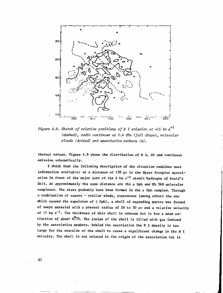
260

220

190

140

100

u j u

X

j >.J —(/

\>

i ; i

I J * U

X

*i/K**\ •

' W • •

vjC3 X

1

g u

Xx

i

1\\r

i

1 !

1 J

-

X

-

_

\

-

3580 35iO 35D0 3i6C 33BD

-1Figure 4.9. Sketch of relative positions of H I emission at -12 tan s~

(dashed), radio continuum at 2.3 GHz {full dvcasn)3 molecular

clouds (dotted) and assoaiation members (x).

thermal nature. Figure 4.9 shows the distribution of H I, OH and continuum

emission schematically.

I think that the following description of the situation combines most

information available: at a distance of 170 pc is the Upper Scorpius associ-

ation in front of the major part of the 4 km s"1 atomic hydrogen of Gould's

Belt. At approximately the same distance are the p Oph and Kh 569 molecular

complexes. The stars probably have been formed in the p Oph complex. Through

a combination of causes - stellar winds, supernovae (among others the one

which caused the expulsion of r, Oph), a shell of expanding matter was formed

of swept material with a present radius of 20 to 30 pc and a relative velocity

of 17 km s"1. The thickness of this shell is unknown but it has a mean ex-

tinction of about 0?75. The inside of the shell is filled with gas ionized

by the association members. Behind the association the H I density is too

large for the rearside of the shell to cause a significant change in the H I

velocity. The shell is not related to the origin of the association but is

82

younger in age. Shells around associations occur more frequently. Examples are

Orion OBI, Cep 0B3 and Mon OBI. They are seen either as a ring of H I or as a

ring of ionized matter. No comparative study has been made of them yet.

The projected length of the streamers is about 18 pc. Because no velocity

gradients are visible along the streamers, we probably look almost perpendicu-

lar to them. I expect the age of the total cloud complex to be at least as

large as that of the OB association and during that time its structure must

have changed. I see three possible ways ("scenario's") of evolution, where

the central question is: how have the streamers been formed, with their struc-

ture that starts right at the center of the p Ophiuchi clouds and extends over

a length of about 18 pc? A first scenario is indicated by Morris et al. (1980)

who observed similar filamentary clouds in CO in Monoceros and Orion. They

proposed that the molecular clouds are moving under the influence of the

galactic gravitational force toward the plane through magnetic flux tubes. In

Ophiuchus this appears to be less plausible: the time scales needed are ̂ 107

years, which is somewhat long. This model can also not explain that the stream-

ers are directed away from the association, the.presence of more than one

streamer and the apparently very coherent structure from the center of the

cloud towards the ends of the streamers. A seaond explanation is that the

origin of the streamers is related to the OB association and the H I shell. In

this scenario the streamers arose from the pressure of the expanding H I shell

which is centered near the association. This feature 2 x 106 yr ago hit the

molecular cloud which was at that time probably closer to the center of the

association and dragged fragments along that were at the outside of this

cloud. The more massive cloud center got a lower velocity and starformation

was initiated in this part of the cloud. The maximum velocity of expansion of

the streamers must have been 9 km s"1. Because there is no velocity gradient

along them, their angle to the lines of sight has to be larger than 80°. The

shell of H I gas appears to have enough kinetic energy to be able to make

this scenario work. A third, somewhat comparable scenario is based on the

models by Woodward (1978), who made calculations of a cloud of 500 M_ which0

was hit by a 21 km s"1 shock front. After 9 million years the cloud shows a

long drawn structure of about 10 pc and a region with high densities at the

front side. However, because the mass of the p Oph clouds is much larger than

500 U , the time scales appear to be too long for this process to explain the

streamers. The structure then must be- a relict of the triggering of the for-

mation of the Upper Scorpio association. This can provide enough time but the

83

model does not explain the presence of more streamers. The last two more vio-

lent mechanisms do not explain the good match of the radial velocity of the

streamers and background neutral hydrogen gas, which probably has a much lar-

ger extent along the line of sight. Although it is uncertain whether it will

work, and more modelling is necessary I think the second scenario is the most

probable to explain the structure of the clouds.

4.9. Conclusions.

I have mapped 48 square degrees (or 425 pc ) of the complex of molecular

clouds near p Oph in the two main lines of OH with a beam of 1.5 pc to deter-

mine the large scale structure of the clouds in this area. This is the first

extensive survey of these molecular clouds. The clouds are very fragmented

and the total amount of mass in the area is about (16 ± 6) * 103 M . Two

separate cloud complexes appear to be involved. One with the P Oph cloud as

its main component, and the other associated with Kh 569. The mass of the

p Oph complex is probably nearly equally divided over the main region and the

two streamers. The Kh 569 complex has a somewhat larger distance than the

rest of the clouds and a mass of about 1000 H.. The mean densities of theB

clouds are in the order of nu = 400 to 700 cm"3. Satellite line observationsn2

show that the main line excitation temperatures are equal except probably in

the center of the p Oph cloud. Along the streamers the radial velocity is

constant but an overall velocity gradient is present perpendicular to the

direction of the streamers. The molecular clouds have the same radial veloci-

ties as the background H I. The process of starformation still is continuing

in the same direction as 5 x 106 years ago. The age of the steamers is proba-

bly less (1 to 2 x 10^ years) and their formation is related to a half shell

of expanding matter around the association.

References.-

Appenzeller, I., 1980, in: Starformation, ed. A. Maeder, L. Martinet (Geneva

Observatory).

Baart, E.E., Jager, G. de, Mountfort., P.I., 1980, Astron. Astrophys. 92_, 156.

84

Barnard, E.E., 1927, in: Photographic Atlas of Selected Regions of the Milky

Way, ed. E.B. Frost, M.R. Calvert (Washington DC: Carnegie Institute of

Washington).

Beintema, D.H., 1975, thesis, Groningen University.

Bignami, G.F., Morfill, G.E., 1980, Astron. Astrophys. 87_, 85.

Blaauw, A., 1961, Bull. Astr. Inst. Neth. J5_, 265.

Blaauw, A., 1964, Ann. Rev. Astron. and Ap. 2, 213.

Blaauw, A., 1978, in: Problems of Physics and Evolution of the Universe

(Academy of Sciences of Armenian SSR, Yerevan).

Blitz, L., 1978, thesis, Columbia University.

Blitz, L., 1980, in: Giant Molecular Clouds in the Galaxy, ed. P.M. Solomon,

M.G. Edmunds (Pergamon Press).

Bok, B.J., 1956, Astron. J. 6j^ 309.

Bujarrabal, V., Nguyen-Q-Rieu, 1980, Astron. Astrophys. 91_, 283.

Cohen, M., Kuhi, L.V., 1979, Astrophys. J. supp. 4£, 743.

Crutcher, R.M., 1973, Astrophys. J. J85_, 857.

Elias, J.H., 1978, Astrophys. J. 224_, 453.

Encrenaz, P.J., Faigarone, E., Lucas, R., 1975, Astron. Astrophys. 44_, 73.

Falgarone, E., Gilmore, W., 1981, Astron. Astrophys. 95, 32.

Garrison, R.F., 1967, Astrophys. J. 147, 1003.

Heiles, C.E., 1969, Astrophys. J. JL57, 123.

Heiles, C.E., Habing, H.J., 1974, Astron. Astrophys. Suppl. _1A.» '•

Heiles, C.E., Katz, G., 1976, Astron. J. 8_1̂, 37.

Khavtassi, J.Sh., 1960, Atlas of Galactic Dark Nebulae, Tiblisi, Abastumani

Astrophys. Obs.

Lynds, B.T., 1962, Astrophys. J. Supp. 7_, 1.

Myers, P.C., Ho, P.T.P., Schneps, M.H., Chin, G., Pankonin, V., Winnberg, A.,

1978, Astrophys. J. 220, 864.

Morris, M., Montani, J., Thaddeus, P., 1980, in: Interstellar Molecules, ed.

B.H. Andrew, p. 197.

Olano, C.H., Poppel, W.G.L., 1981, Astron. Astrophys. 95_, 316.

Ross, F.E., Calvert, M.R., 1934, Atlas of the Northern Milky Way, (the Uni-

versity of Chicago Press).

Sancisi, R., Van Woerden, H., 1970, Astron. Astrophys. 5_, 135.

Seeger, C.L., Westerhout, G., Conway, R.G., Hoekema, T., 1965, Bull. Astr.

Inst. Neth. _18_, 11.

Strauss, F.M., Pöppel, W.G.L., Vieira, E.R., 1979, Astron. Astrophys. 7\_, 319.

Turner, B.E., 1973, Astrophys. J. 186, 357.

85

Vidal-Madjar, A., Laurent, C., Bruston, P., Audouze, J., 1978, Astrophys. J.

223, 589.

Vrba, F.J., 1977, Astron, J. 82, 198.

Woodward, P.R., 1978, Ann. Rev. Astron. and Astrophys. 16, 555.

86

CHAPTER V

OH OBSERVATIONS OF THE TAURUS COMPLEX

5.1. Abstract.

In this chapter I present the results of OH observations of two complexes

of molecular clouds in the Taurus region. 180 Square degrees have been mapped

in the main lines of OH and at some ten positions also the satellite lines

were measured. In section 5.2 I give a general introduction of earlier obser-

vations. In sections 5.3 and 5.A I present the method of observing and the ob-

servational results. In section 5.5 the observations are analysed. First I

compare them with earlier OH and with CO observations and with A , , the

amount of photographic extinction. Second, column densities and masses are

derived. The general velocity structure of the two complexes is discussed in

section 5.6 and in section 5.7 the OH observations are compared with data on

starformation in these areas.

5.2. Introduction.

One of the areas in the Northern hemisphere best known for dark clouds

is situated below the galactic plane in the constellations Taurus, Perseus and

Auriga. This collection of clouds, probable belonging to Gould's Belt will

hereafter be referred to as the Taurus complex. The complex has an extent of

at least 20 in longitude and latitude but probably the clouds are not all at

the same distance. Through photographs the numerous clouds were described and

named by Barnard (1927), Khavtassi (1960) and Lynds (1962). Figure 5.1.a shows

a sketch of the clouds in this area, composed of the results of these authors.

Hatched lines denote heavy obscuration, full drawn lines indicate areas where

the different results agree. Near the dashed lines the extinction is probably

much weaker and differences between the Lynds and Khaytassi maps occur. Best

estimates of the borders of the clouds are drawn in these cases. Also shown

are some emission and reflection nebulae. The area counts many of these

87

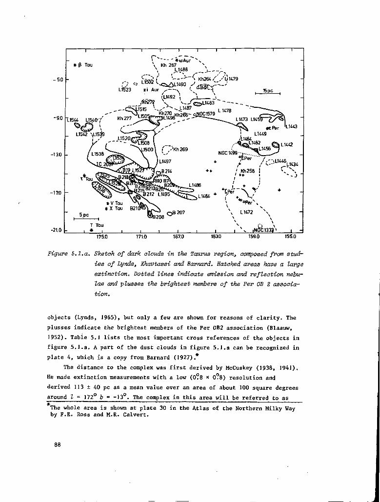
-5 .0

-9.0

-13.0

* ( J Tau \ Kh 267J.J4B8

' xi Aur ̂ >

Kh26t/'/UK79

, 15pc |

175.0 171.0 167.0 163.0 159.0 155.0

Figure 5.1.a. Sketch of dark clouds in the Taurus region^ composed from stud-

ies of Lynds, Khavtassi and Barnard. Hatched areas have a large

extinction. Dotted lines indicate emission and reflection nebu-

lae and plusses the brightest members of the Per OB 2 associa-

tion.

objects (Lynds, 1965), but only a few are shown for reasons of clarity. The

plusses indicate the brightest members of the Per 0B2 association (Blaauw,

J952). Tabie 5.] lists the most important cross references of the objects in

figure 5.J.a. A part of the dust clouds in figure 5.J.a can be recognized in

plate 4, which is a copy from Barnard (1927).*

The distance to the complex was first derived by McCuskey (1938, 1941).

He made extinction measurements with a low (0?8 * 0?8) resolution and

derived 113 ± 40 pc as a mean value over an area of about 100 square degrees

around I = 172° b = -13°. The complex in this area will be referred to as

The whole area is shown at plate 30 in the Atlas of the Northern Milky Wayby F.E. Ross and M.R. Calvert.

88

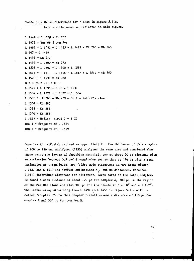
Table 5.1. Cross references for clouds in figure 5.1.a.

Left are the names as indicated in this figure.

L 1449 + L 1459 = Kh 257

L 1472 = Per OB 2 complex

L 1487 = L 1482 + L 1485 + L 1487 = Kh 263 + Kh 265

B 207 = L 1489

L 1495 = Kh 271

L 1497 + L 1500 = Kh 273

L 1508 = L 1507 + L 1508 + L 1514

L 1515 = L 1513 + L J5J5 + L 1517 + L 1539 = Kh 280

L 1520 + L 1539 = Kh 282

B 218 to B 211 = DL 1

L 1529 + L 1535 + B 18 = L 1531

L 1534 = L 1527 + L 1532 + L 1534

L 1535 to B 208 = Kh 279 = DL 2 = Kuther's cloud

L J536 = Kh 285

L 1538 = Kh 286

L 1540 = Kh 288

L 1534 = Heiles' cloud 2 = B 22

TMC 1 = fragment of L 1534

TMC 2 = fragment of L 1529

"complex A". McCuskey derived an upper limit for the thickness of this complex

of 100 to 150 pc. Adolfsson (1955) analysed the same area and concluded that

there exist two layers of absorbing material, one at about 50 pc distance with

an extinction between 0.5 and 4 magnitudes and another at 170 pc with a mean

extinction of 1 magnitude. Bok (1956) made starcounts in two areas within

L 1521 and L 1534 and derived extinctions A , but no distances. Heeschen

(1951) determined distances for different, large parts of the total complex.

He found a mean distance of about 100 pc for complex A, 300 pc in the region

of the Per 0B2 cloud and also 300 pc for the clouds at b = -8° and I < 167°.

The latter area, stretching from L 1492 to L 1456 in figure 5.1.a will be

called "complex B". In this chapter I-shall assume a distance of 110 pc for

complex A arid 300 pc for complex B.

89

Large-scale 2] cm line observations were made by Sancisi and Wesselius

(1970). Assuming a uniform spin temperatures of 125 K they found an anti-cor-

relation between H I and dark clouds. In addition indications of H I selfab-

sorption were found in two areas at two velocities. In one of these areas one

of the first detections of molecules in dark clouds was made by Heiles (1968)

who detected OH in the part of L 1534 that he called "Cloud 2". Cloud 2 has

subsequently been observed by many authors looking for a large variety of

molecules. In general complex A is particularly remarkable for the long chain

molecules (HC..N, HC.,N) which were detected in some of its small, dense clouds

(TMC 1, TMC 2, L 1544, L 1521, Walmsley et al., 1980). Molecular observations

of a large area of the Taurus complex were first made by Sancisi et al. (1974),

who observed the Per OB 2 cloud in OH. Sargent (1979) made CO observations of

the same cloud. Baran (private communication) has observed the whole Taurus

complex from 1 = 155 to Z = 190 in CO with the 1.2 m Columbia telescope, but

the results have not yet been published. Rydbeck et al. (1976) made CH obser-

vations at a number of disconnected positions in the Taurus complex. Crutcher

(1973) and Heiles and Katz (1976) observed OH and H„C0 along the dust lanes

(DL 1 and DL 2).

Massive star formation has occurred only in the cloud, near the Per OB 2

association, which has a photometric age of about 6 x 106 year. The kinematic

age is a factor 4 smaller. The distance of the association (350 pc) is about

the same as that of the clouds. The runaway star XI Per originated in this

association; it probably has a larger distance and excites the H II region

NGC 1499 (the California Nebula). Complex A, at 110 pc has only a few embedded

B stars and a large number of T Tauri stars: starformation has led to less

spectacular results. Cohen and Kuhi (1979) recently estimated the age distri-

bution of these stars. A study of the relation between T Tauri stars and

molecules was made by Lang and Willson (1979) and by Herbig (1977). Jones and

Herbig (1979) determined the proper motions of the T Tauri stars. Elias (1978)

observed in the near infrared a part of the clouds to see if there are embedded

objects associated with the clouds. Van Duinen (private communication) found

a far infrared source near TMC 1. There are a number of Herbig-Haro objects

within the clouds (Herbig, 1974).

A part of complex A was mapped with a low sensitivity in OH by Baud and

Wouterloot (1980; see chapter 2 of this thesis). These observations were not

sensitive enough to draw accurate conclusions about the optical depth and

about eventual line ratio anomalies. Also the velocity resolution was not good

90

-5.0

-9.0

I-13.0

-17.0

-21.0

eXXX XX

xxxxxxxxxxxxxxxxxxxxx

xxxxxxxxxxxxxX' XXXXXXXXXXXXX

xxxxxxxxxxxxxXXXXXXXXXXXXXXXXX X

. xxxxxxxxxxxxxxxxxxx/xxxxxxxxxxxxxxxxxxxxxxxxxxxxxxxxxxxxxxxxxxx

X XXXXXXXXXXXXXXX XX

XXXXXX

-mxxxxxxxxxxxx xX XXXXXXXX XXXXXXXXXX XXXxxxxxxxxxxxxxxxxxxxx

xxxxxxxxxxxxxxxxxxxxxxx xxxxxxxxxxXXXXXXXXXXXXXX XXxxxxxxxxxxxxxxxxxxxxxxxxxxxxxxxxXXXXXXXXXXXXXXXXXXXXXXXXXXXXX

XXXXXXXXXXXXXXxxxxxxxxxxxxx xxxxxxxxxxxxxxxxxxxxxxxxx:xxxxxxxxxxx

xxxxxxxxxxxxxxxxxxxxxxxxx

-W,

<xxxxxx«xxxxxxxxx<xxxxx:

XXXXXXXXX KXXXXXXXXXXXXX

xxxxxxxxxxxxxxxxxxxxx"

xxxxxxxxxxxxxxxxxxxxx

XX XXXXXXXXXXXXXXXXXXXXXXXXXXXxxxxxxxxxxxxxxxxxxxxxxxxxxxxxxxxxXXXXXXXXXXXXXXX

XXXXXXXXXXXXXX

xxxxxxxxxxxxx(XXXXXXXXXXXXXXXXXXXX

xxxxxxxxxxx xxxxxxxxxxxxxxxxxxxxxxxxxxxxxxxxxxxxxxxxKXXXXXXXXXXXXXXXXXXXxxxxxxxxxxxxxxxxxxxxcxxxxxxxxxxxxx

xxxxxxxxxxxxSX XXXXXXXXXXXxxxxxxxxxxxxxx xxxxxxxxxxxs. XXXXXXXXXXXX•vXXXXXXXXXXXsxxxxxxxxxx

XXXXXXXXXXXXXXXXXXXX X XxxxxxxxxxxxxxxxxxxxxxxxxX X X X X X X X X X X X X X X X X X X X X Xxxxxxxxxxxxx xxxxxxxxxxxxxxxxxxxxxxxxxxxxxxxxxxxxxxxXXXXXXXXX XXXXXXXXXXXXXXXXXXXXX XXXXXXXXX

X XXXXXXXXXX XXXXX Xx xxxxX XXXXX

xxxxx; xxxxXXXXX

xxxxxxxxxxxxxxxxxxxxXXX

XXXXXXXXXX XXXXXXXXXXXXXXXXxxxxxxxxxxxxxxxxxxxxxxxxxxxxxxxxxxxxxxxxxxxxxxxxxxxxxxxxxxxxxxxxxxxxxxxxxxxxxxxxxxxxxxxxxxxxxx h"XXXXXXXXXXXXXXXXXXXX XXX

xxxxxxxxxxxxxxxxxxxxx.XXXXXXXXXXXXXXXXXXXXXX

xxxxxxxxxxxxxxxxxxxxXXXXXXXXXXXXXXXXXX XXxxxxxxxxxxxxxxxxxxxxx

XXXXXXXXXXXxxxxxxxxxxXXXXXXXXX

XXXXXXXX

KXXXXXXXXXX«xxxxxxxxxx«xxxxxxxxxxxx

XXXXXXX XXX XXXXXXXXXXXXxxxxxxxxxxxxxxxxxxxxxx

XXX XXXXXXXXXXXXXXXXXXXXXXXX XX

XXXXXXXXXXXXXXXXX

XXX

I

179.0 175.0 171.0 167.0 163.0 159.0 155.0

Figure 5.1.b» The positions observed in OH indicated with a cross with the

outlines of the different regions3 to be discussed in section

5. 4. Complex A consists of region e to I and complex B of region

a to d*

enough to determine the velocity structure of the complex. Therefore I reob-

served in J978 a small part of the complex with better resolution and longer

integration times. This improved the quality of the observations so much that

I decided to observe the whole Taurus complex in OH.

5.3. The observations•

I observed with the Dwingeloo telescope (beam 3J1) simultaneously the two

main lines at positions that formed a 0?3 x 0?3 grid. The resolution was

91

0.9 km s"1 except at a few positions around (J76°, -11°) where it was 0.45

km s"1. The integration time was 30 minutes per position in the total power

mode, which resulted in a r.m.s. noise of about 0.02 K. The total area of the

Taurus complex covers at least 400 square degrees, a too large area to observe

in the time available. Therefore I choose to observe the area of the complex

as detected in CO (Blitz, J980) and to trace the borders of the OH cloud in

the parts where the OH is more extended. To decrease a possible bias against

areas where OH exists but no CO, I observed a number of cross cuts outside the

CO cloud. Also *:he experience in other areas has shown that OH always coexists

with CO. A total of J930 positions was observed in the main lines (see figure

5.1.b) requiring approximately 3500 hours of observation time (reference

measurements included), spread over J979 and 1980. The area of the Per OB 2

cloud had already been observed sufficiently by Sancisi et al. (1974) and was

observed again at only a few positions to check the temperature scale. At 17

positions with a high value of T , the satellite lines were observed to im-A, J

prove the knowledge of the excitation conditions within the clouds. These

observations were made in the frequency switched mode with an integration time

of 4 hours and a resolution of 0.9 km s . The spectra, in which the line

appeared in signal and reference band were subsequently folded and added.

5.4. The observational results.

The observations reveal the presence of a large number of discrete emis-

sion regions with a mean size around two to three parsec, embedded in an ex-

tended area of low level emission. In figure 5.2 I show the peak antenna tem-

perature in the complex at 1667 and 1665 MHz. The typical distance between the

individual "> 0.1 K" peaks is about 3 parsecs. The peaks are generally aligned

along structures with a length of about ten parsecs. Lack of observing time

prevented me to observe some outer parts of the complex where the peak emis-

sion becomes smaller than 0.04 K. I will indicate later in section 5.5.2 where

this happened. There are no unexpected differences between figures 5.2.a and

5.2.b. There is no position where the strength of the 1665 MHz line is excep-

tionally strong, as expected for a maser source. The upper limit for such a

source is about 0.4 Jy. This upper limit can be compared with the strengths

of other maser sources. W3(0H) (25 times farther away) has components between

100 and 200 Jy and the Cep A OH maser (7 times farther away) shows emission

92

-5 .0

-9.0

-13.0

-17.0

- 2 1 . C _L _L179. 175.0 171.0 f 167.0 163.0 159.0 155.0

Figure 5.2.a. Peak antenna temperatures at 166? MHz. Contourvalues are 0.05,

0.09, 0.13, ... K. Positions from table 5.2 are indicated.

between 5 and 20 Jy, both in addition to weaker components. I think it is

fairly certain that the Taurus complex does not contain a maser source. The

results at some individual positions will be shown and discussed in section

5.5.2.

Figure 5.3 shows I, the integrated line intensity at 1667 and 1665 MHz.

A comparison of figure 5.3 and figure 5.2 can give information about variati-

ons in linewidth and about the reality of some cloud components. With the

present resolution (0.9 km s"1) all spectra show only one component at each

position. Higher resolution observations by Turner (1973) indicate that in

some cases the line is split. The velocity structure of the complex will be

discussed in section 5.6. Figure 5.12 shows that most emission in complex A

is concentrated at 6 and 7 km s"1 but that higher and lower velocities are

93

-5.0 -

-9.0

i i i i i

-17.0

-21.0

179.0 175.0 171.0 167.0 163.0 159.0 155.0

Figure 5.2.b. The same as figure 5.2.a at 1665 MHz. •

present especially at the edges. Complex B shows emission between -8 km s~J

and 0 km s"1; the higher velocities occur at the highest longitudes. The com-

plexes overlap around (168°, -7°) and are clearly separated in velocity. This

agrees with the results by Heeschen (1951), who finds absorption in this area

at 115 and at 300 pc distance.

5.5. Analysis.

5.5.1. Comparison with earlier observations, with CO and extinction.

The present observations are an extension of the observations described

in chapter 2. Figure 2.5 can directly be compared with figure 5.2. In both

-5 .0

-9 .0

-13.0

-17.0

-21.0

i i i r

J L179.0 175.0 171.0 $ 167.0 163.0 159.0 155.0

Figure 5.3.a. Integrated line intensity at 1667 MHz. Contourvalues are 0.10,

0.18, 0.26, ... K.

figures the general outline of the main cloud is the same. Due to the better

sensitivity there are differences in parts of the clouds where the emission

is weaker. In the area around (J7J°, -10°) the clouds look less fragmented in

figure 5.2 than in figure 2.5, which was made with the same sampling. In the

old observations the temperatures appear to be almost a factor two higher. A

few new observations at positions in the Per OB 2 cloud which has been ob-

served previously with a comparable telescope at Onsala (Sancisi et al., 1974)

indicate that the new temperature scale is the correct one.

Figure 5.4 shows an enlargement to the same scale as figure 5.2 of a

recent contour map of integrated CO temperatures (Baran, private communicati-

on) . The CO have been observed with the Columbia telescope (beam 7!5) with a

sampling that varied between 7'.5, in areas of strong emission, and ]° in areas

95

-5.0 -

-9.0 -

i I I i i i I i i i i i i

-17.0

-21.0179.0 175.0 171.0 167.0 163.0 159.0 155.0

Figure S.3.b. The same as in figure 5.3.a. at 1665 MHz.

where no CO was detected. The map looks rather different from that in an ear-

lier publication (Blitz, 1980} for reasons unknown to me. CO was observed with

a low velocity resolution of 2.6 km s'1.

The general outlines of the OH and CO clouds are the same: the extent of

the molecular clouds appears to be well defined. This will be discussed in more

detail in section 5.5.4. The CO clouds scattered outside the main complex were

not observed in OH due to lack of time. I made some crosscuts outside the CO

clouds at I = 165?J, at b = -12?1 and at b = -U?7 in addition to a few smaller

ones. No OH was detected in these regions, which indicates that the borders of

the OH cloud really have been found. However, in view of the large CO sampling

distance of i degree in the region around (165° - 12°) I think it is not ex-

cluded that there are still some small clouds in this area.

96

-5.0 -

-170

-21.0175.0 171.0 167.0 163.0 159.0 1550

Figure 5.4. Integrated line intensity of CO (from Baran^ private communicati-

on). Contourvalues are in units of 2 K hn s

There are some differences between OH and CO. In some regions the CO is

more extended than the OH; in particular this occurs at (169°, -17°). Also

the minimum at (+173 , -12 ) is more pronounced in OH than in CO. This reflects

a higher CO abundance, since instrumental effects (beam smearing) will produce

opposite results. There is one region near (174°, -11°) where the OH extent

appears to be larger, and this then can have been caused by the larger OH beam.

In general the CO shows less pronounced peaks than the OH. The structures

have the same angular extent as in OH in spite of the difference in beamsize!

It may be that the structure is "smeared" by the larger CO optical depth. A

remarkable result of the CO observations is that by far most of the T Tauri

stars in the area (see section 5.7) fall within the 6 K km s"1 contours,

whereas the correlation with the 'corresponding' 0.3 K km s"1 contours of OH

97

-3.0 -

-9.0

i i i i i

-13.0 -

-17.0 -

179.0 175.0 171.0 1670 1630

Figure 5.5. Photographic extinction (from McCuskey, 2938). Contourvalues are

0j 0.4, 0.8 ... magnitudes.

is less convincing. This may have been caused by a local heating of the gas by

the T Tauri stars. However the actual CO temperatures are not known, apart

from some incidental observations (e.g. Milman, J975) where temperatures be-

tween 3 and 8 K were found. It will be important to make far infrared searches

in these areas to get more information on the grain temperatures. Other heating

sources are probably responsible for some other significant CO peaks that are

much weaker or absent in OH, e.g. those near (158 , -12 ) and (167 , -3 ).

I will now compare the molecular maps with those of the photographic ex-

tinction, made by McCuskey (1938) through starcounts with an angular resolution

of 0.8 in a part of the observed area. Figure 5.5 shows his extinction values

presented in new galactic coordinates. For clarity only half of the original

contours are drawn. Figure 5.5 shows a good resemblance to figure 5.2 and 5.4.

98

0.02 -

0.00 -

- 004

- 0 00

0.00

- 032

- 0 00

20.0 0 0 km/s - 1 0 0

Figure S.6.a.

L-174 4 b=-13 6

000

• 0.32

-0 .16

-OiOO

200 10-0K m *

200Km/s

Figure 5.6.b.

99

L=175° 3 b= -16°-6

0.02 •

0.00

OJ04

' I ' 1 I i I I • I

0.000.00

20-0 10-0 200 10-0 Km/s •40O

Figtwe 5. 6,a. A few sample spectra of all 4 lines at three positions.

The OH cloud becomes visible between extinction values of 0.2 and 0.8 magni-

tudes, the higher number occurs in areas without dust lane features in the

upper and middle right part of complex A. A more quantitative comparison of

'-he three maps will be made in section 5.6.

5.5.2. Analysis of satellite line observations.

I made observations of the satellite lines at 17 positions in the cloud

complex. These positions are situated at or close to main line peaks and are

indicated in figure 5.2.a. The results of the observations are listed in

table 5.2. Some typical spectra are shown in figure 5.6. The velocity resolu-

tion is the same in all spectra, except in some spectra around (176 , -11 )

where the main line resolution is a factor two better. The observations at .

these J7 positions were analysed in the way discussed in chapter J. The re-

sults are displayed in table 5.3.

I will first make some general comments. The values for T_, T „, Nnu,

T . and T . in table 5.3 are for P = J, DT = 0 and TD. = 3.4 K. In mostex,1 ex,4 BGcases the filling factor has no effect on the predicted values of T. . and

A, i

T. ,. At three positions, indicated.with an asterisk, the fit is slightly

better for a somewhat lower value of F (0.4). Determination of a significant

100

Table 5.2. Observed parameters.

b

T

VAV

TA 2V

AV

TA, 3V

AV

TA,4V

AV h I ,i

157.0

161.5

168.7

169.9

171.1

171.4

1 7 1 . 7

1 7 2 . 6

173.8

174.4

174.6

174 9

- 8.8

- 8.5

-14.Ö

-11.2

-14.5

-16.3

-13.6

-10.5

0.044-7.3

1.5

0.104-3 .2

1.8

-15.4 <0.015

-19.3 <0.015

0.0826.71.3

9.7 -0.0357.21.2

0.0375.81.1

0.0296.01.5

-0.0205.81.1

0.1295.71.1

-0.0467.60.8

-0.0217.01.5

-10.8 -0.0296.91.0

0.105-7.0

2.1

0.122-2.82.0

0.1857.31.3

0.0678.51.0

0.1456.61.2

0.0856.82.0

0.1305.91.5

0.2026.31.4

0.0966.31.8

0.2636.31.5

0.0916.22.5

0.0936.22.0

0.130 0.029-7.1 -5 .81.7 2.5

0.155-2.6

1.7

0.2537.31.5

0.1698.61.1

0.2316.61.2

0.1566.91.7

0.1656.21.7

0.3456.31.3

0.1946.71.3

0.3556.31.7

0.1546.81.0

0.1696.31.2

<0.015

0.1387.71.2

0.0518.31.2

0.260

0.217

0.299

0.066

<0.010 0.247

not 0.163observed

0.0526.81.7

0.0676.41.3

0.0866.21.5

0.1786.51.3

0.0816.33.1

0.0606.91.4

0.214

0.314

0.443

0.163

0.121

0.242

0.216

0.359

0.180

0.305

0.184

0.347

0.484

0.116 0.337

0.609

0.271

0.278

101

Table 5.2 continued.

TAI b V

. AV

1 TA,V

AV

2T

A,3V

AV

TA,4V I,

AV1 h

175.2 -12.3 -0.042 0.170 0.201 0.191 0.264 0.4006.3 6.0 6.0 6.31.7 1.3 1.5 1.4

175.3 -16.6 -0.023 0.101 0.176 0.050 0.153 0.2746.4 6.0 6.0 6.01.4 1.4 1.4 1.7

175.5 -12.6 -0.055 0.182 0.243 0.222 0.273 0.3806.3 6.0 6.3 6.21.4 1.2 1.2 1.4

175.5 -10.2 <0.015 0.071 0.150 0.053 0.133 0.2556.1 6.1 6.31.8 1.5 1.7

176.1 - 9.9 0.041 0.121 0.161 0.061 0.107 0.2633.8 6.9 7.0 6.21.3 0.9 1.2 2.0

upper limit for DT is only possible if the apparent T, is relatively high;

otherwise the predictions are insensitive for DT variations. If F < 1, the

upper limits for DT remain valid. At 7 positions no definite value could be

obtained for T , and T ,; a large temperature interval is possible. Com-ex,l ex,4 ö r

bining table 5.2 and 5.3 one deduces that at positions with a high antenna

temperature (T. , > 0.20 K) in 80% of the cases also a relatively high T,

(£ 1.0) is derived. However, the reverse seems not always true: three positi-

ons with a high T, occur when T. . is low. But since two of these three posi-

tions are in the larger distance complex B, this does not argue against a

correlation between T. . and T». There is no correlation between high T_

values and the CO intensity in figure 5.4: a part of the OH positions with a

high T. fall outside CO maxima. There is a weak indication that high T- values

occur preferentially at positions with a larger extinction. The mean extinc-

tion (derived from figure 5.5) at positions where T, > 1.0 equals A . =

2.1 ± 0.5 magnitudes, and where T. < 1.0 equals A , = 1.6 ± 0.8 magnitudes.

The only position in table 5.2 where I could not make a one component

fit of the observed satellite line antenna temperature is at (174.4, -13.6)

in Heiles cloud 2. The 1612 MHz spectrum in this case shows a peculiarity in

the form of absorption at 7.6 km s"1 and emission at 5.7 km s"1. The mean

102

Table 5.3. Derived OH parameters.

T. T • N..„xlO14 T T , DT3 ex, 3 OH ex, 1 ex,4

157,

161.

168.

169.

171.

171.

171.i

172.

173.

174.

174.

174,

175.

175.

175.

175.

176.

.0

,5

.7

,9

1

4

7

6

8 *

4

6

9

2

3

5*

5

1*

- 8.

- 8.

-15 .

-19.

-14.

- 9.

- 1 1 .

-14.

-16.

- 1 3 .

-10.

-10.

-12 .

-16 .

-12 .

-10 .

- 9.

.8

,5

,4

3

8

7

2

5

3

6

5

8

3

6

6

2

9

1#5-C

3±1

2±1

<0.5

<1.0

K 5 -o0.5±0

<0.3

2.5±1

<1.0

<1.0

3.5±1

<1.0

3

<0.2

3 1

i .5

6

.5

.5

3.7±0.1

3.6

3 .8

>4.0

3.8±0.1

>3.8

3.7

>4.0

>4.3

3.9

>3.7

>3.8

3.7

>3.7

3.7

>4.5

3.7

2.5+10

40±10

30±10

2±1

5±4

20+10

7 5

2.5+1.5

20±10

10±8

6±4

50±10

8±5

3.5

2+1

30±10

3.8

4 . 4

3.4

-

4.5±0.5

3

3.7

-

-

-

-

3 .2

-

3.1

-

3 .5

3 .5

3 .5

4 . 3

-

3.4

-

3 .6

-

-

see text

-

-

4 . 4

-

4 . 5

-

3.7

<0.2

0

0

-

0 .5

-

0

-

-

-

-

0

-

0

-

0

velocity is close to that of the main lines, especially in view of the resolu-

tion. The 1612 MHz structure was also detected with better velocity resolution

by Turner (1973) at his position 2D. Perhaps in this cloud two partly overlap-

ping components are present with different excitation conditions. However the

observations by Turner also show that the mainline and 1720 MHz intensities

are very difficult to separate into two components. Probably the line does not

consist of two components at overlapping velocities, but an excitation differ-

ence exists at the two velocity sides of the satellite lines. The main lines

have the same excitation temperature. A fit is T = 4.3 K, T , = 3.4 K atSX ) J GX f 1

103

V < 6.3 km s'1 and T = 3.1 K, T = 4.6 K a t V > 6.3 km s" 1 . The f i r s t6 X y 1 63C y H

situation, T . > T /is less common in OH clouds. At most of the positions

where an accurate fit could not be made of T , and T ., I obtain Tex,1 ex,4 ex,]

< |T ,|. This also is theoretically the most probable situation in dust

clouds (see Guibert et al, 1978): only if the dust temperature is high, they

predict T . > T .. It will be interesting to see why only the high velocity

side of the lines at position (174.4, -13.6), and also at some neighbouring

positions observed by Turner, show this excitation. Van Duinen (private commu-

nication) detected a far infrared source in this area and one part of the

cloud may have been heated more than the other part. It is possible that the

cloud is contracting with a velocity of about 0.5 km s"1 and heated for some

reason (T Tauri stars?) at the front side of the cloud. However, no significant

temperature enhancement is visible in the CO maps by Baran. The alternative is

that there are two OH clouds with the same main line excitation conditions and

about the same column densities. This situation is suggested by the H_CO ob-

servations by Sume et al. (1975), who found two clouds with different veloci-

ties. Position (174.4, -13.6) is in the region of overlap of the two clouds.

It remains necessary to heat one of the clouds. A similar situation exists at

one position L 1626 (see chapter 3) where the two velocity sides of the cloud

appear to have different excitation conditions in the satellite lines.

5.5.3. Analysis of main line observations.

In this section I shall analyse the main line ratios in different parts

of the cloud complex. In the whole Taurus complex I measured this ratio at

some 1200 positions. This number is too large to allow analysis position by

position. Also the error in each individual measurement is too large to make

an accurate estimate of T„. Therefore I made a statistical analysis of the OH

properties in each of 12 regions whose boundaries are shown in figure 5.1.b.

There is a large number of quantities that one can study.

1. The mean optical depth in different areas.

2. The optical depth within one area as a function of antenna temperature.

3. The linewidth within one area as a function of antenna temperature.

4. The relation between mean T- and A . .

5. The relation with satellite line data.

6. The relation of excitation conditions with the eventual occurrence of star-

formation in the area.

104

7. A comparison with other molecular data.

During the analysis I firstly have made figures in which are plotted a. T. „A,i

versus T, „; b. Io versus Io; c. T. _ versus I_ and d. T. o versus I_. In someA,3 2 3 A,2 2 A,3 3

cases the plotted quantities were averages over up to 4 adjacent positions,

where the results are expected to be similar. Secondly I have calculated, in

intervals of 0.05 K, the mean value of the ratios of the above properties. This

resulted into a total of 48 tables and figures. Here I show only the most im-

portant ones, and I summarize briefly the other results. Table 5.4 gives the

main results of the mean observational properties in the different regions. In

column 4 is the number of positions with T. , > 0.05 K in the area. Column 5

and 6 contain R 3 T. ~/T. „ and RT = I,/Io. Columns 7 and 8 contain the line-A,3 A,2 1 3 2width, derived from IQ/T. _ and I9/T. 0. The uncertainty in linewidth is in all

j A, j *• A, Z.

cases about 0.3 km sT^ .

For all 12 regions, R is almost equal to R although mostly slightly less.

This is also to be expected for lines where the optical depth in the line

center is higher than in the wings. R../R will vary from 1.00 at T. = 0 to 1.13

at T. = 3, but the effect is too small to be recognized quantitatively in table

5.4. Since I have concluded in 5.5.2 that DT - 0, I suggest that the values

of R points in many regions to a substantial optical depth, up to T . = 2 in

region 1. The mean linewidth is nearly equal at 1665 and 1667 MHz. It varies

between 1.9 and 2.9 km s"1. There are no systematic trends in the sense that

the linewidth is higher in areas with a lower or higher T. ,.A, J

I will now discuss the individual regions.

Region a only shows very weak, but definitely real emission. It is located

near the open cluster NGC J342, which has a distance of about. 550 pc (Johnson

et al. 1961), but probably there is no genetic relation betwaen dust clouds

and clusters whose age is (8 ± 3) * 108 years (Gray, 1965). The dust clouds

(listed as L 1434 by Lynds (1962)) consist of a number of small {y 20') frag-

ments which are separated from the other complexes in the surrounding. The

extinction A in front of the cluster is about 0.84, the same value as found

by Heeschen (1951) in that general direction. Heeschen determined a distance

for the cloud of 300 (± 100) pc. The radial velocity of the OH emission, about

0 km s"1, adds no information about the distance and for the present time I

will adopt 300 pc. Because the lines are too weak I cannot determine T,, and

1 assume T~ = 0 and T = 5.5 K. The mean OH column density is then 1.4 x 1011*

cm"2 and the mass is 500 Mg. This is probably an overestimate because the

fragments are smaller than the beam.

105

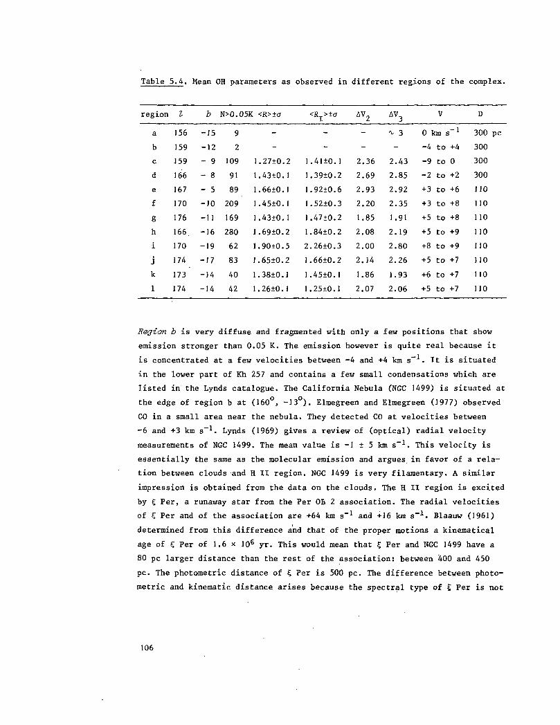
Table 5.4. Mean OH parameters as observed in different regions of the complex

region

a

b

c

d

e

f

g

h

i

j

k

1

I

156

159

J59

166

167

170

176

166.

170

174

173

174

b

-J5

-12

- 9

- 8

- 5

-10

-11

-16

-19

-17

-14

-14

N>0.

9

2

109

91

89

209

169

280

62

83

40

42

05K <R>±CT

-

-

1.27±0.2

1.43±0.1

1.66±0.I

1.45±0.1

1.4310.1

1.6910.2

1.90+0.5

1.6510.2

1.38+0.1

1.26±0.1

<R >±a

-

-

1.41±0.1

1.39+0.2

I.92±0.6

1.52+0.3

1.47+0.2

1.84+0.2

2.26+0.3

1.66+0.2

1.4510.1

1.25+0.1

AV2

-

-

2.36

2.69

2.93

2.20

1.85

2.08

2.00

2.14

1.86

2.07

AV

<v

2.

2.

2.

2.

1.

2.

2.

2.

1.

2.

r

3

3

43

85

92

35

91

19

80

26

93

06

V

0 km

-4

-9

-2

+3

+3

+5

+5

+8

+5

+6

+5

to

to

to

to

to

to

to

to

to

to

to

s"1

+4

0

+2

+6

+8

+8

+9

+9

+7

+7

+7

D

300 pc

300

300

300

110

110

110

110

no110

no110

Region b is very diffuse and fragmented with only a few positions that show

emission stronger than 0.05 K. The emission however is quite real because it

is concentrated at a few velocities between -4 and +4 km s"1. It is situated

in the lower part of Kh 257 and contains a few small condensations which are

listed in the Lynds catalogue. The California Nebula (NGC 1499) is situated at

the edge of region b at (160 , -13 ). Elmegreen and Elmegreen O 977) observed

CO in a snail area near the nebula. They detected CO at velocities between

-6 and +3 km s"1. Lynds (1969) gives a review of (optical) radial velocity

measurements of NGC 1499. The mean value is -1 1 5 km s~1. This velocity is

essentially the same as the molecular emission and argues in favor of a rela-

tion between clouds and H II region. NGC 1499 is very filamentary. A similar

impression is obtained from the data on the clouds. The H II region is excited

by £ Per, a runaway star from the Per OB 2 association. The radial velocities

of £ Per and of the association are +64 km s"1 and +16 km s - i. Blaauw (1961)

determined from this difference and that of the proper motions a kinematical

age of 5 Per of 1.6 x 106 yr. This would mean that £ Per and NGC 1499 have a

80 pc larger distance than the rest of the association: between 400 and 450

pc. The photometric distance of £ Per is 500 pc. The difference between photo-

metric and kinematic distance arises because the spectral type of £ Per is not

106

accurately known, but it can be decreased if one assumes that the star is

slightly evolved (Bohnenstengel and Wendker, 1976). The only uncertainty then

is the distance of the clouds. Heesschen (1951) determined 300 pc for both

region b and c. He does not include an estimate of the uncertainty, but it

might be considerable. Furthermore region b and c are not necessarily at the

same distance because a velocity gradient in region b prallel to the galactic

plane (to be discussed later) is not found back in region b. I conclude that

the following situation probably exists: from the Per OB 2 association at

350 pc distance, the star £ Per was expulsed 1.6 * 106 yr ago with a velocity

of 50 km s"1. The star now has reached a distance of 400 to 450 pc where it

met a very filamentary system of small clouds with an overall size of about

25 pc. ? Per ionized a part of the clouds which is visible as NGC 1499. To

confirm this one has to obtain the distance of the small clouds near NGC 1499

through starcounts. The molecular mass in region b is probably not larger than

a few hundred solar masses.

The CO maps (see figure 5.4 and Blitz, 1980) show relatively strong

CO in regions a and b. The weak OH can be explained by a filling factor

F much smaller than 1 and the strong CO by a higher kinetic temperature

than the other clouds.

Region o and d have to be regarded as one cloud system because of the similar

radial velocities. I have divided it into two parts only to see whether the

conditions vary over the complex. This cloud system consists of a relatively

narrow (1.5) chain of clouds with a number of maxima, about 2.5 apart. At the

highest longitudes (I = 169 ) this region overlaps partly with the clouds in

region e, but the velocity difference of 4 to 5 km s points out that two

separate cloud systems are involved.

The cloud is optically not well defined at the less negative latitudes,

see figure 5.1.a. It contains a few high extinction Lynds clouds. Heeschen

(195]) derived a distance of 300 pc in this region. This number is not very

accurate, but it is the only determination available; a kinematical distance

is not reliable. There are no bright stars associated with this complex. The

star e Per, with a distance of 2J0 pc shows no

expected velocity (Marshall and Hobbs, 1972) and is thus a foreground star.

At the distance of 300 pc the length of the complex (13 degrees) is 70 pc,

similar to the long chains of clouds which Morris (J980) found in Orion and

Monoceros. The complex contains the small nebula NGC 1579. It is brighter

blue light than in red, so probably it is a reflection nebula. The extinction

107

_ L=155.5-163.0

B=-10.9—7.3

0.1

0.0 -

0.0 0.11667 MHZ TP

0.2

Figure 5.7.

Plot of T. „ against T. _ in region

a. Lines of x = 0 and x =

indicated.

are

within the complex is known, only from Heeschen's somewhat inconclusive re-

sults. He finds a mean value of > 2.3 magnitudes.

The mean optical depth in region c is T = 1.9 + 0.5 and in region dT3 "» 1.7 ± 0.6, essentially the same. This is relatively high in view of the

low antenna temperatures in this area, T does not seem to very with T

(see figure 5.7); within the errors the line ratio is constant. I shall assume

one excitation temperature for the whole region, because the accuracy of ob-

servations and theory does not justify to calculate it at every individual

position. The value obtained in the cloud center is T , = 3.64 K. In reality

I do not expect that T and T , are constant over the whole cloud. An inter-

esting object situated behind the clouds is 3C 11J, a radio galaxy with an 18

cm flux density of about 14 Jy, which enabled me to obtain (very local) data

on the excitation temperature (see farther down). The only position where a

more accurate determination of the excitation temperature could be made is in

front of 3C 11J. A previous measurement with the Nancay telescope at this

position at 1667 and 1665 MHz by Dickey et al. (198J) gave an absorption line

around -2 km s"1. At the higher velocity resolution at J667 MHz, line was

found to consist of two separate components at -1 and -2.5 km s"1, with the

same mean excitation temperature of T _ = 4.8 K. I show ray Dwingeloo measure-

ments in figure 5.8. This is a velocity-longitude diagram through 3C 111,

whose position is indicated. Figure 5.8 shows emission and absorption features

at this position at 1667 MHz. The 1665 MHz spectra are similar. Since 3C 111

is definitely behind the cloud, the presence of the both emission and absorp-

tion requires that the cloud has two components with different excitation

temperatures. With the two sets of measurements I can calculate T , and T_ex, ó j

108

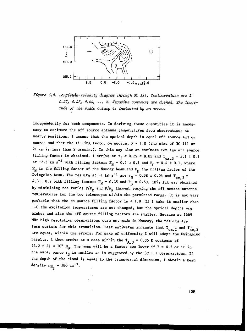
160.D -

2.0 0.0 -2.0 -1.0 Vkm/è

Figure 5.8. Longitude-Velocity diagram through 3C 111. Contourvalues are ±

0.G5, 0.071 0.09, ... K. Negative contours are dashed. The longi-

tude of the radio galaxy is indicated by an arrow.

independently for both components. In deriving these quantities it is neces-

sary to estimate the off source antenna temperatures from observations at

nearby positions. I assume that the optical depth is equal off source and on

source and that the filling factor on source, F = 1.0 (the size of 3C 111 at

21 cm is less than 2 arcmin.). In this way also an estimate for the off source

filling factor is obtained. I arrive at T = 0.29 ± 0.02 and T = 5.1 ± 0.1_i ex,3

at -2.5 km s with filling factors F„ = 0.5 ± 0.1 and Fn = 0.4 ± 0.1, where

FN is the filling factor of the Nancay beam and FD the filling factor of the

Dwingeloo beam. The results at -1 km s"1 are T O = 0.38 ± 0.04 and T3 ex,3

4.3 ± 0.2 with filling factors FH = 0.25 and FD = 0.50. This fit was obtained

by minimizing the ratios F/FD and F/FN through varying the off source antenna

temperatures for the two telescopes within the permitted range. It is not very

probable that the on source filling factor is < 1.0. If I take it smaller than

1.0 the excitation temperatures are not changed, but the optical depths are

higher and also the off source filling factors are smaller. Because at 1665

MHz high resolution observations were not made in Nancay, the results are

less certain for this transition. Best estimates indicate that T „ and Tex,2 ex,3

are equal, within the errors. For sake of uniformity I will adopt the Dwingeloo

results. I then arrive at a mass within the T. = 0.05 K contours of

(4.2 ± 2} x 101* M@. The mass will be a factor two lower if F = 0.5 or if in

the outer parts T 3 is smaller as is suggested by the 3C 111 observations. If

the depth of the cloud is equal to the transversal dimension, I obtain a mean

density n H = 180 cm"3.

109

Region e corresponds with the area of the dust clouds L 1492 and L J488 in

figure 5.1.a. The clouds in this region are not very well defined and 'show

only weak OH emission. Figure 5.1 indicates that the clouds have not been

mapped fully at the lowest longitudes. However Baran (see figure 5.4} detected

no or only very weak CO emission in this area so the most important part has

been observed. Heeschen (1951) assigned a distance of 300 pc to this area but

the velocity in the upper part of region e is quite different from region d

for which he assigned the same distance. Eklöf (1958) found in this area dis-

tances of 115 and 300 pc for two dust clouds with comparable extinctions. I

find these clouds back around (J67 , -7 ) where I detected emission at two

velocities. One cloud is the end of complex B and the other cloud at about

+5 km s~ extends through the rest of region e. This probably is the cloud at

115 pc distance which belongs to complex A, because the velocities are similar

to those in region f. The lines are weak and a determinatie-. • T_ is not well

possible. It is certainly not very high and I will assume T_ although R

is somewhat lower than 1.8. At a distance of 310 pc the total mass of all

clouds in this region is (8 ± 4) * JO2 Mfl.

Region ƒ through 1. This is a very extended area in which the dark clouds pro-

bably form one entity as shown by the radial velocities: for the largest part

the velocity is constant within 1 or 2 km s'1. With the present velocity reso-

lution no splitting of the lines are seen, so no clouds with velocities which

differ more than 1 km s"1 are situated behind each other. Only a mean distance

is known, about 310 pc. Those of individual parts were not determined and the

three dimensional structure is not clear. Part of the complex is characterized

by a structure of long, relatively narrow dust lanes (like the streamers in

the Ophiuchus clouds). In particular these are situated in the lower part of

figure 5.1.a. At lower (less negative) latitudes (region f and g) the optical

structure is more that of a number of scattered clouds, embedded in a common

envelope. This resembles the structure in Orion where also the part farthest

away from the plane is best defined (see chapter 2). The CO map by Baran

(fig. 5.4) also indicates that I mapped this part of complex A fully; only

some smaller clouds visible at distances of more than 2 degrees from complex

A, have not been observed.

Region f. Lynds (1962) lists a number of high extinction clouds within region

f (see figure 5.1.a), which are partly detected in OH (figure 5.2). I find an

average optical depth of T. = 1.0 a 0.4, which does not vary significantly

with T. .. T „is equal to 3.77 K in the cloud center. There is one other

no

determination of T in the area near the quasar 3C 123, which is situated

near the edge of the dust cloud L 1507. It is seen as a minimum at (170.5,

-11?5) in figure 5.2.a. The extinction in front of 3C123 is A = 1.5 to 2.0

magnitudes. Nguyen-Q-Rieu et al. (1976) derived T , = 5.5 ± 0.5 K and

T „ = 6.5 + 0.5 K. Also Crutcher (1977) found that in this cloud the twoex, 2

excitation temperatures are possibly different. Since in section 5.5.2 I have

shown that in the cloud center DT = 0 I will use in first instance this result

for the whole cloud. Then the mass of the clouds in region f is (4.4 ± 2)

x 103 M . Here the mass fraction in the low level emission where 3C 123 is

situated is between 50% and 70%. The total mass changes to 2.8 x 101* M if in

this part the 3C 123 data are adopted. The mass fraction in the small clouds

at the low latitude side of region f which possibly not have been mapped fully

is very small.

Region g is separated from region f by an area of weak emission. Also the CO

and the extinction map justify a separate discussion of this region. It forms

the apparent end of a rather narrow structure starting around (165 , -17 )

that runs over 14° (or 30 pc) to (177°, -10°). The velocity maps show (see

section 5.6) that it is split into a number of different, but probably nearby

features. Optically this region is not very well defined (see figure 5.1.a).

It has one very dense core (L 1544) at (178 , -10 ) where cyanopolyynes have

been detected (Walmsley et al. 1980). However this dust cloud is too small to

resolve with the Dwingeloo telescope. One of the maxima at (175 , -13°) does

not show up in the CO map (figure 5.4), but A , has a maximum at that position

(figure 5.5). In this maximum the optical depth of OH is perhaps slightly

higher than in the rest of the cloud, but the uncertainties are so large that

the distribution of R as a function of T _ also can be caused by a single

value o;. T_ = 1.4 ± 0.5. This means an excitation temperature in the cloud

. center of T = 3.83 K and a mass in region f of (2.1 ± 0.5) x 103 M_. Thisex,3 ° 0

value does not change much if part of the cloud has a higher T_ or if the low

level emission has a lower value of T,. An indication that the latter may be

the case is obtained from absorption measurements against the radio continuum

source 3C 133 (Kazès et al., 1977). Because this is a relatively weak source

I saw in Dwingeloo very weak emission at this position and I obtain in the

same way as before for 3C 111, T = 4.0 ± 0.1 K, T, = 0.65 ± 0.05 andex, j 3

F a 0.5. T , is equal within the errors to T _, however I assign lessex,£ ex,J

weight to these results than to those of 3C 111.

Ill

Reg-ion h is the low longitude part of the earlier mentioned narrow structure.

Compared to the other regions (a - g, i - 1) it is rather large, but since

the conditions appear quite uniform I treated it as one entity. Optically it

consists of a number of narrow dust lanes (see figure 5.1.a), but the OH map

shows that these lanes are more extended; they are embedded in a large area

of low level emission. There is a maximum in T _ > 0.25 K, but in contrast

with the other regions which contain such high values of T , region h doesA, j

not show a high mean optical depth, T~ = 0.3 ± 0.3. The observaions at posi-

tion (171.1, -14.8) indicate (see section 5.5.2) T~ = 1. OH observations have

been made previously by Lang and Willson (1979) in the direction of T Tauri

stars that are seen projected at some of the dust lanes. They detected

emission which is about a factor two stronger than what I observed but this

is because the dust lanes are smaller than the Dwingeloo beam. For my observ-

ations I estimate 0.5 < F < 1. However outside the maxima F may be closer to

1. The line ratios of Lang and Willson generally point to i. = 1, in agree-

ment with my determination in the cloud center. I adopt T„ = 1.0 at the posi-

tions where T. , > 0.2 K and T~ = 0.3 in the other parts of the cloud, I then

arrive at a mass of (3.9 ± 1.5) x 103 M@.

Regions i and j contain another narrow dust lane stretching from (170 , -19 )

to (J75 , -15 ). It has an extension, probably of lower density, which is

seen as a weak emission nebula that extents in the direction of the Pleiades

(see Lynds, 1965). Both objects are probably not directly related because of

the large age of the Pleiades and the different space velocities of the

Pleiades and the T Tauri stars in the Taurus cloud (Jones and Herbig, 1979).

The dust lane is rather fragmented and some parts of it (the Barnard objects

208, 210, 215 and 18 in figure 5.1.a) show up as maxima in the OH. The dust

lanes are not as conspicuous in CO as in OH. This can be a consequence of a

higher optical depth in CO, but also of a higher temperature in the more dif-

fuse parts. I have divided this dust lane in two parts, the regions i and j.

Region i. This is one of the parts of the cloud complex where the extinction

very neatly follows the OH contours. The line ratio R in region i is large,

which points toward a low optical depth and I will assume T_ = 0. The mass

within this region is then (5.5 ± 2) x 102 Mfl.

Region j consists of the second part of the dustlane in region i and another,

parallel dustlane (L 1536). The upper dustlane (L 1529) contains the dense

condensation TMC 2. The number of positions is too small to treat both parts

separately. The line ratio's indicate an optical depth of x_ = 0.4 ± 0.3, also

112

in the cloud center. This means a mass of (1.4 ± 0.6) x 103 M , about one

third of which is in L 1536.

Regions k and I have the highest antenna temperatures in the Taurus complex.

Also the highest extinction in figure 5.5 is in these regions. They contain

the dust clouds L 1521 and L 1534. TMC 1 and Heiles cloud 2 are situated in

L 1534. The clouds are not as narrow in these regions as in the regions h, i

and j. They are the central and best studied regions of the Taurus complex.

However they are less dominant than the p Oph area in the Ophiuchus complex.

Region k. Both regions show a relatively low line ratio, independent of T

(see figure 5.9).A,3

"i i r

L=172.0-173.2

B = -15.«—13.3

1 r

R = 1.0

(0.2

0.1

0.0 -

R=1.8

0.0 0. 1 0.2 0.316S? KHZ TP

Figure 5.9. Plot of T against 2^ g in region k. Lines of x = 0 and x =

ars indicated.

The optical depth is expected to increase with T ^ , because the regions are

bounded by areas with lower T 3 and T^y It is difficult to find the transi-

tion between two such areas, but at least the transition from region h to

region k appears to be fairly sharp. Some high extinction areas in region h

and k have been investigated earlier by turner and Heiles (1974) who correlated

113

OH and H„CO observations with measurements of A^. They found a mean optical

depth of 2 to 3 in region k and in the center of region h. Turner and Heiles

concluded that To is independent of A^. This is also partly the result of my

observations (see the constancy of R in figure 5.9), it will be discussed in

more detail later in this section. I obtain a mean value of x, = 1.5 ± 0.5 in

region k. Then the mass within that part of the cloud is (9.4 + 0.3) x 103 M .

Region I was observed in OH with a beam of 18 arcminutes by Heiles and Gordon

(1975) at a number of positions. Their line profiles showed in

some cases 2 or 3 components with a different velocity. My velocity resolution

is too poor to see this splitting. H„CO observations with a smaller beam by

Sume et al. (1975) showed that there are some fragments within this cloud

with sizes of the order of a few arcminutes. However high resolution OH observ-

ations do not show line intensities above 0.7 K so probably the filling factor

of my beam is not below 0.5. The optical depth in region 1 is 2.2 + 0.6 and

the mass is (1.0 ± 0.2) x 103 Mffl. This value is in agreement with Wilson and

Minn (1977) who found about 103 M. in cloud 2. Because the mass is highly frag-0

mented all my estimates of column densities will be somewhat too high in the

cloud centers, but I expect this not to be the case in the outer parts of the

cloud. The largest error will be the uncertainty of the adopted constant op-

tical depth.

The derived properties are summarized in table 5.5. The total mass of

complex A (regions e to 1) is (1.5 ± 0.5) x 101* MQ and of complex B (essenti-

ally region c and d) is (4 ± 2) x 10** M . Minimum values for the masses are

respectively 9.4 x 103 and 1.1 x JO1* M . The masses are probably in error by

less than a factor 2 due to a filling factor F < 1. The mean density in column

8 of table 5.5 is derived for the average extent of the clouds in the differ-

ent regions. If I estimate the mean densities in the clouds with equation (1.1)

and the derived excitation temperatures, I obtain the same general results as

in table 5.5 provided that the kinetic temperature of the c]cuds is about 5 K.

This result is not very significant because equation (1.1) is a very crude

approximation. The "peak" density in column 7 of table 5.5 is derived from

the column density in the cloud center and the apparent extent of the cloud

core. This number is very uncertain, but it will give an indication of the

variation of mean densities which occur on the scale of a few parsec. There

are not much other determinations of the density in this area. Walmsley et al.

(1980) derive for the clouds where cyanopolyynes have been found a value of

114

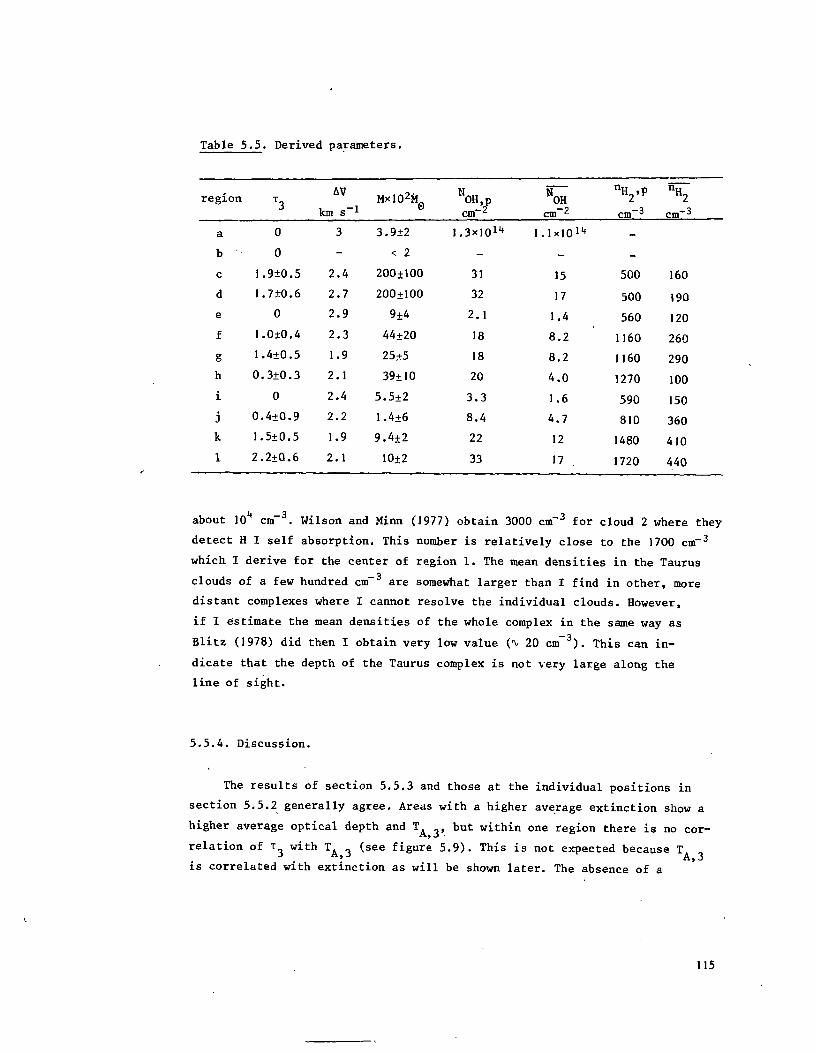
Table 5.5. Derived parameters.

A V MxlO2M NOH

a

b

c

d

e

f

g

h

i

j

k

1

1

1

1

1

0

0

1

2

0

0

.9±0

.7+0

0

.0+0

.4±0

,3±0

0

.4±0

• 5±0

.2+0

.5

.6

.4

.5

.3

.9

.5

.6

3

-

2.4

2.7

2.9

2.3

1.9

2.1

2.4

2.2

1.9

2.1

3.9±2

< 2

200+100

2OO±1OO

9±4

44±20

25+5

39±10

5.5±2

1.4±6

9.4+2

10+2

1.3xli

-

31

32

2.1

18

18

20

3.3

8.4

22

33

500

500

560

1160

1160

1270

590

810

1480

1720

160

190

120

260

290

100

150

360

410

440

r e g i o n T 3 _ MxlOzM@ OH,p "OH 2tan s ' * cm~* cm~2 cm"3

L l x l O 1 4

15

17

1.4

8.2

8.2

4.0

1.6

4.7

12

17

about 101* cm"3. Wilson and Minn (J977) obtain 3000 cm"3 for cloud 2 where they

detect H I self absorption. This number is relatively close to the 1700 cm"3

which I derive for the center of region 1. The mean densities in the Taurus

clouds of a few hundred cm"3 are somewhat larger than I find in other, more

distant complexes where I cannot resolve the individual clouds. However,

if I estimate the mean densities of the whole complex in the same way as

Blitz (1978) did then I obtain very low value (% 20 cm" 3). This can in-

dicate that the depth of the Taurus complex is not very large along the

line of sight.

5.5.4. Discussion.

The results of section 5.5.3 and those at the individual positions in

section 5.5.2 generally agree. Areas with a higher average extinction show a

higher average optical depth and T A ,, but within one region there is no cor-

relation of T with T „ (see figure 5.9). This is not expected because TJ A»-3 A,3

is correlated with extinction as will be shown later. The absence of a

115

UI

X

oz

2.

1.

0.

0

0

0

1

-

x

- i *

1 1

)

X )

J^XJ$

• i

<x

i

X

X>

>

1

X

f X

IX

1

1

M

x̂

1

X

<X

1

1

-

X

X^ ^

0.0 1.0 2.0RPH MHG

3.0

Figure 5.10. Plot of NQE against A ,. The two lines indicate an OH abundance

of 2 x lCT7 (lower! and 4 x 10~7 (upper line).

correlation between T_ and extinction was also found by Turner and Heiles

(1974), who observed a much smaller region. However because Turner and Heiles

derived OH optical depths only at positions with a very limited range in ex-

tinction, their results are not really conclusive. This can also be the cause

of the apparent constant R in the regions k and 1: the mean extinction varies

only with ] magnitude. I think this is a observational problem, which can only

be solved by observing a simple cloud at a number of radially distributed po-

sitions with such an accuracy that, for each position, R can be determined

within 0.05 to 0.1. However this is a program which will need very much observ-

ing time. Turner and Heiles (1974} and Heiles and Gordon (J975) discuss the

relation of OH, H,C0 and A . I --a make a comparison of OH, CO A , and CH overi. v pn

a much larger area. The analy. ••he first three species was made by di-

viding the figures 5.2.a, 5.3.a, 5.4, „.5 and a similar figure of NrtU (calcu-uti

lated with the results in table 5.5) in 0.5 x 0.5 squares and reading off the

values at about 500 positions. These numbers were averaged over ]° x i° areas

and compared with each other. The results are displayed in table 5.6 and figure

5.10. In general there exists a correlation between each of the quantities but

mostly the spread is large. When they are compared one has to bear in mind

that the data are taken over a very extended area with a low resolution. In

some cases the correlations appear to be better for smaller regions, e.g. the

116

Table 5.6. The correlation of two quantities (A and B).

A -

XC0

JcoTA,3

h~N0H

TA,3

B .

"V-h- A .

ph

ph

- A ,ph

- TCH

A -

2.01

1.29

0.17

0.028

(0.05

0.014

x + y B

+ 1.31 A .ph

+ 15.9 I 3

+ 0.051 A .ph

+ 0.107 A ,ph

+ 4.53 A , ) x JO11»ph

+ 0.50 T. 0A,3

r2

0.14

0.44

0.47

0-54

0.58

0.72

CO shows higher temperatures in the area around (168°, -15°), which makes the

general correlation worse. From table 5.6 one can see that the correlations

involving CO are the least good, probably because the lines have a high opti-

cal depth. Because of this reason it is very difficult to reach more accurate

conclusions. The isotope * CO was only measured at a few positions. The corre-

lation of OH and A . appears to be fairly good. This confirms the results of

Turner and Heiles and of Sancisi et al. (J974). Turner and Heiles observed in

two small areas (5 sq. degrees in total) with a high mean extinction and a

high mean T (about 2.5). Sancisi et al. observed the Per 0B 2 complex where

both extinction and T are lower. If antenna temperatures are converted to

brightness temperatures the slope of the T_„ - A , relation appears to beUn pn

different, 0.129 (Turner and Heiles), 0.108 (Sancisi et al.) and 0.067 (my re-

sult). The data in Per 0B 2 and in Complex A were obtained with a similar

telescope, and the extinction data are both from McCuskey (J938) so the differ-

ence may be real. Perhaps this difference can be explained by a higher mean

gas temperature in the Per 0B 2 cloud, as it is found from CO observations.

The data by Turner and Heiles were obtained with a very different beam and a

different velocity resolution, both of which tend to increase the slope if

clumps are present. In figure 5.10 I show the correlation between N„„ and A , .OH . ph

It appears to be nominally better than that between I. and A , (I, is propor-

tional to the column density of OH when T_ = 0 and T „is constant over the

cloud). In figure 5.10 I have drawn lines of different OH abundances, calcu-

lated with A = 0.75 A and N„ (tot) = 2 x ]021 A . I obtain in this way av pn n v '

117

mean abundance of (3 + 1) x 10~ . This is an upper limit for two reasons: A .

is underestimated in areas with a high extinction because of the lower spatial

resolution of the original observations and because of the rather bright mag-

nitude limit (15 ). The mean value of N n o per beam can only be lower and neverUtt

higher because of probable lower filling factor. If this is taken into account

the deviation of the observed abundance is not very much off the adopted rela-

tion (1.7). Also the variation of abundance with T_ that I have assumed appears

compatible with figure 5.JO; positions with a high i. are preferentially lo-

cated in the upper part of figure 5.10. According to table 5.6 there exists

a very straight relation between T , and T . The CH data are from Hjallmar-

son et al. (1975), who observed it at a number of positions in the complexes

A and B. Since CH is optically thin at all positions, one expects that the

T „/T ratio is smaller at positions of higher x, than at positions of

lower T„. This is not the case. The explanation, which I prefer, is that the

CH abundance is smaller in the cloud centers than in the rest of the clouds.

I derive a CH/OH abundance ratio which varies from O.I at small T, to 0.05

at higher T.. This confirms the results of Hjalmersson et al. (1975) whose

absolute numbers are somewhat larger (the average abundance ratio is 0.2).

The alternative explanation is that T_ is small at all positions, which will

mean that the abundance ratio of OH and CO is constant. It will be important

to derive column densities of other molecules (CO, H„CO, CH) at a larger

number of positions in order to get a hint of (variations of) abundance ratios

in these clouds. Such ratios can then be compared with model clouds as a check

on cloud chemistry.

Blitz (1980) has shown that for large molecular clouds there exists a

relation between the cloud surface within a certain CO temperature contour and

that CO temperature: log A a 0.16 T„rt AV. Figure 5.11 indicates that a similar

relation also exists for OH. The slopes are almost equal for three of the com-

plexes. Only for Complex A it is somewhat different. The deviations from a

straight line for the Ophiuchus complex are caused by the p Oph area, where

relatively high antenna temperatures occur in a small area. The lines in

figure 5.11 indicate that the extent of the clouds is well defined although

they can be somewhat larger than I have found (a factor two for complex A).

I' do not think that this extrapolated extent is real: dumpiness will enlarge

the extent of the low level emission and increase the slope. I shall return

to the results in figure 5.11 in chapter 8.

118 .

1000

100

Areapc?

10

x Tau Complex A• Tau Complex Bo Ophiuchus

OB1

0.05 0.10 0.15 0.20 0.25 0.30 0.35

2

'Figure 5.11. Plot of the cloud surface in pc against T. , for four complexes.

5.6. The velocity structure of the Taurus complex^

Figure 5.12 shows the 1667 MHz OH emission at constant, velocities, in

intervals of 1 km s"1 between -8 and +9 km s~^. Because the total cloud com-

plex can be separated into two parts this analysis will be divided similarly.

Firstly I will describe the velocity structure in complex B. Secondly complex

A will be analysed.

119

-3.0

-9.0

-15.0

-21.0

-3.0

-9.0

15.0

21.0

3.0

9.0

15.0

21.0

1

_

-

-

-

-

1-8.0

X

X

-6.0

X

X

1.0

X

X

1KM/S

11

KK/S

KM/S

1

X

X

X

X

11

X

X

X

X

11

X

X

X

X

1 1

I I

X

X

X

11

X

X

X

X

X

X

1 1 1

X —

X —

X ( X

X —

1 1

1

T1

1-7.0

X

X

5.0

X

X

-3.0

X

X

1

1KM/S

KVS

/s

1

X

X

X

X

11

X

X

X

X

11

X

o

X

X '

X

1 1

1

X

X

X

11

X

X

X

1

1

X

X

X

1

1 1

Xb

0

X

1 1

1

_

l x "

X —

-

_

X

-

X —

1 -1

-

X

X —

179.0 173.0 167.0 161.0 155.0 173.0 167.0 161.0 155.0

Figwee 5.12.a.

120

-3.0

-9.0

-15.0

- 2 1 . 0fr"

r r i i i : i i \ i i-2 .0 KM/S

X . X •» X

^r-H—1—I—I—h

i i r-1 .0 KH/S

i i r

0.0 KH/S 1.0 KH/S

tel

m- 9 . 0

- 1 5 . 0

- 2 1 . 0

-3.0

-9.0

-15.0

X «X

i 1 1 F T - H 1 1 1 1 f-

• • < * -

2 . 0 KM/S 3.0 KH/S

X . X

' . 4.J

•Jk —

- 2 1 . 0 I I I I I J L

x * •

J I I L J L179.0 173.0 167.0 161.0 155\0 173.0 167.0 161.0 155.0

Figure 5.12.b.

121

-15.0 -

ri 1 1" ~\ 1 1 h f

- 2 1 . 0

179.0 173.0 1G7.0 161.0 155.0 173.0 167.0 161.0 155.0

F-pgure 5.22.C. 1667 MHz antenna temperatures at velocities between -8 and +9

hn s~l. Contour values are 0.04, 0.06, 0.08, 0.10, 0.125,

0.150, 0.175, 0.20, 0.25, 0.30 and 0.35 K. Some positions are

indicated for reference purposes.

122

170.0

1S6.0

162.0

158.0

~T 1 1 T

-3.0 Vkm/s

Figure 5.13. Longitude-velocity diagram at b = -8.5. Contourvalues are 0.0Z,

0.063 0.09, ... K.

Complex B. There are two indications that complex B is separate. Distance

estimates for this part are around 300 pc whereas the distance of the rest of

the cloud complex is about 110 pc and in the region of overlap with complex A

at (168 , -7 ) there is a clear velocity separation of about 5 km s"1 (see

figure 5.12). Although complex B and the Per 0B 2 clouds (a small part is

visible in figure 5.12 at 6 and 7 tos"1 around (161°, -19°)) are at about the

same distance, their velocity is about JO km s"1 different so at present they

are spatially and kinematically disconnected. The main structure of complex B

can be seen in figure 5.13. This is a longitude velocity diagram at b = -8?5.

It shows a large velocity gradient of 8 km s"1 from about -8 km s"1 at

I = 157 to 0 km s~a at I = 166°. At a distance of 300 pc this corresponds to

a period of 3.4 x 107 yr if the gradient is explained by rotation. The size

of the gradient is the same as in several other cloud complexes (chapter 2, 4),

but the sense of the rotation is unusual, because it is in the same direction

as galactic rotation. In principle such velocity gradients can also be ex-

plained in other ways. Streaming motion is one of these, but I think this is

123

less probable because it means that either the complex is longer than the

projected 70 pc, or the real velocity gradient is very large. Furthermore I

see no direct cause of such streaming motion parallel to the galactic plane.

The rotation is not necessarily really solid body rotation; it might be more

resembling a shearing motion. From figure 5.13 and 5.12 I have the impression

that complex B is built up from a number of individual clouds with sizes of

the order of 5 to 10 pc (1 to 2 ) each of which has a constant velocity. An

indication for this structure is also given at the position of 3C 111 (Z- =

161.8) (indicated by arrows in figure 5.13) where the absorption spectra show

two overlapping cloud fragments. In the major part of the complex the H I vel-

ocities are rather different from those of OH. This is not expected because

most molecular cloud complexes are associated with a large H I cloud. Probably

the H I at the molecular velocity is hard to see because of the huge contri-

bution of atomic hydrogen at positive velocities with a large linewidth. This

hydrogen is more local, and associated with the molecular complex at 110 pc

distance.

The velocities in region b are somewhat less negative than in region c.

Most emission is at about -4 km s . This cloud is very fragmented. The

difference in velocity between the two regions can indicate that they are not

connected. In region b, near NGC 1499, also some emission is present at +4

km s"1. The emission in region a is strongest at 0 km s"1. The weakness of the

emission in the regions a and b prevents further conclusions about the veloci-

ty structure therein.

Complex A. The rest of the Taurus complex shows emission between +4 and

+10 km s"1. The velocity structure appears to be fairly complicated. The most

important result is that complex A as a whole has no large velocity gradients

along the line of sight, contrary to complex B and many other clouds. Most

emission is at +6 and +7 km s"1 in the center of the complex and higher velo-

cities occur at the two opposite sides. At the region of transition between

complex A and the Per OB 2 cloud complex (at £ = 1 6 2 , £ = - 1 7 ) one can see

a velocity jump of 2 km s"1 from +8 to +6 km s~^. Both regions do not overlap

and have a velocity gradient in the opposite direction. So the two complexes

are not connected, which is not unexpected in view of the difference in dis-

tance. Although there is no verall velocity gradient, it is clear that many

of the individual peaks which are visible in figure 5.2.a have different

velocities, with, however a small dispersion of the order of 2 km s"1 around

a mean value of about 6 km s"*. In some cases it is difficult to distinguish

124

between a local velocity gradient and the presence of separate clouds. An

example of a possible velocity gradient is given by the clouds in region g at

b = -10 , where a gradual shift from 6 to 8 km s is visible. However in

figure 5.2.a this continuous ridge can be recognized as a series of different

peaks. I think this difficulty to distinguish is typical: the large scale

structure of a cloud may show a velocity gradient but the individual parts

have a constant velocity within the present resolution. This behaviour is

clearly demonstrated in several of the dust lanes. Consider first dust lane

DL 2 (in the nomenclature of Clark et al., J977), extending in figure 5.1.a

from L 1535 to B 208. Crutcher (1973) observed a few positions within DL 2 and

showed that there is a velocity gradient along this dust lane. However the

optical appearance is that of a series of clumps (see figure 5.1.a). Figure

5.12 shows that each of these fragments has, within the present resolution,

a constant velocity: B 18 at 6.5 km s"1, B 215, B 212 and B 210 at 8 km s"1

and B208 at 8.5 km s"-1. An other clear indications of the constancy of the

radial velocity along a dust lane is that the small lane below DL 2, L 1536

has a constant velocity of 6 km s-i. The dust lane DL 1 is very narrow and

extends from B 217 to B 209 in figure 5.1.a. The OH beam is too large to sepa-

rate this dust lane from the nearby cloud L 1521 in the maps of peak antenna

temperature (figure 5.2). However the position of DL 1 is coinciding with a

maximum in figure 5.3.a at (169.5, -16 ). This indicates that thp linewidth

at this position is larger than around b = -15 . This increase in linewidth

can be caused by an extra cloud component in addition to L 1521 with a veloci-

ty that is only slightly different. A large velocity difference is ruled out

because the lines in this area are not split. The velocity of this component

can be deduced from figure 5.J2, where a feature is present at +6 km s

which coincides exactly with DL 1. Since the emission at the position of DL 1

at +7 km s is equally strong I conclude that DL 1 has a nearly constant

velocity of 6.5 km s"1. Earlier observations of the velocity structure in

these dust lanes were made by Heiles and Katz (J976) who observed with high

resolution a number of positions along the dust lanes DL I and DL 2 in H„CO.

Their general result is the same as that found in the present observations:

the dust lanes show changes of velocity, but these are not smooth. The veloci-

ties in individual condensations within the dust lanes tend to be fairly con-

stant. In addition they found at several positions two velocity components.

The velocity resolution of the OH observations is too small to detect these

components. The velocity structure in other parts of complex A is less clear,

125

e.g. in the relatively isolated region e an increase in velocity is visible

from +4 km s"1 to +6 km s"1 in an irregular way, roughly from the lower right

to the upper left corner.

The OH velocity in most cases generally agrees with that of the H I

(Heiles and Habing, 1974), but if it is looked at in detail, one can see dif-

ferences up to 2.5 km s"1. These differences do not occur very systematically.

This probably means that the clouds are embedded in a large H I cloud with

mean velocity variations of the order of a few km s"1, but those of the denser

parts of this complex can be somewhat larger.

The velocity structure is probably to be explained by the way the Taurus

complex originated. It has been noticed by others that there seems to be an

almost circular overall structure of the Per OB 2 complex, complex B and

complex A. Heiles and Katz (1976) suggested that the three complexes have a

common origin which is perhaps related to the H I shell, found by Sancisi

(1973) near the Per OB 2 cloud. This shell and the circular structure would be

swept up by a supernova remnant somewhere in between the present complexes.

However such a common origin seems to be rather improbable to me in view of

the large differences in distance between e.g. Per OB 2 (300 pc) and complex

A (100 pc), the large mass involved (about 105 M_) and the distribution of

velocities over the three complexes. I think that a discussion of an eventual

relation of these three complexes has to be made within the scope of a discus-

sion of the structure of the local arm, including features like Goult's Belt

and other complexes. For example one thing overlooked in previous models

(e.g. Weaver, J974), where the velovxty distribution of H I along the galac-

tic plane was related to an expanding ring of gas, is that (a part of?) the

gas around V = 150 to I = 180 at +5 to +7 km s"1 is related to the Taurus

complex and not to the part of the expanding ring at a distance of 300 pc.

Of the two individual complexes A and B, the only one of which enough is

known to discuss its formation, is complex A. Complex A probably is a separate

entity with an age of the order of 107 years, see section 5.7. Such complexes

quite possible grow by coalescence of smaller clouds (Scoville and Hersh,

1979; Kwan, 1979). An indication for this is given by the many smaller clouds

in the neighbourhood of the complex in the CO map (figure 5.4). Such small

clouds are not detectable in other complexes because of the larger distances.

Because coalescence is a very slow process, the beginning of the complex

formation was probably triggered by another event. Also the systematics of the

velocity field appear difficult to explain if random coalescence is the

126

important formation mechanism. A spiral arm shock is not very probable in this

case and one of the remaining possibilities again is a supernova explosion.

Recently Batrla et al. (1981) pointed out from the analysis of H I self ab-

sorption observations that the H„/H I ratio in Oloud 2 and in DL 2 is a factor

10 different. A possible explanation is that DL 2 is a factor two older of a

factor three denser than cloud 2. This, together with their different morpho-

logy can be important. The position of the suggested supernova has to have

been behind the present complex A, because the velocities and line profiles

indicate that the complex is not very extended along the line of sight. At the

position of the complex already existed an extended H I cloud which was part

of Gould's Belt (age about 5 x 107 years, Lindblad, 1974). The evolution of

the supernova remnant had some consequences for the gas in its neighbourhood.

It formed filaments by instabilities in the shell. The example of IC 443

(Duin and Van der Laan) shows that the total mass in the form of cold filaments

can be of the order of 1000 NL with mean densities of about 250 cm"3 and that0

the filaments occur at one side of the remnant. Probably such filaments are

now visible as the narrow dustlanes in the Taurus complex. The masses and mean

densities which I obtained are not too high. The dust lanes are probably formed

in the less dense parts of the H I complex. Other clouds like Cloud 2 are

either already existing H I or molecular condensations within the large cloud

or clouds which have been captured later. In the first case the density was

probably increased by the shock of the passing remnant, however for some reason

no massive star formation was triggered, probably because the distance between

supernova and Cloud complex was rather.large. The radial velocity structure

with higher velocities at both ends also can be explained by an expanding SN

shell. The velocity differences of about 2 km s~ over 10-20 pc distance are

relatively small because of the large H I mass and the large distance of the

supernova. Coagulation can play a small role in the growth of the complex

during the next 107 years. The complex is to old to see a remnant of the shell,

but it still has the morphology of a sheet of clouds: it is relatively thin

(about 5 to 10 pc) in comparison with the extent of about 40 pc.

5.7. Star formation.

Contrary to many other dark clouds the Taurus complexes A and B do not

contain young massive 0B stars. Only stars of relatively late type (B5 - A0)

127

- 8 . 0 -

- 1 2 . 0 -

-16 .0 -

-20.0 -

178.0 1714.0 170.0 166.0

Figure 5.14. Peak antenna temperature at 1667 MHz with T Tauri stars of ages

less than 6 x 10 years (X) and more than 6 x 10 years (L).

are found in the vicinity of the clouds (Elias, 1978). The nearest OB associa-

tion is Per OB 3 at (147°, -6°) with a distance of about 170 pc from the sun,

and 80 to 100 pc from complex A. A doubtful association is Cas Tau 0B 1 at a

distance of about 160 pc between I = 120° and I = 200° below the galactic plane

(Petrie, 1958). Both associations aia poorly studied and on this basis I shall

not try to relate them to the molecular complexes. However complex A has many

T Tauri stars, most of which are concentrated in a number of groups that are

scattered over the complex. Figure 5.14 shows the positions of these stars

(Herbig and Rao, 1974) superposed on the clouds. There is only a weak correla-

tion between cloud properties (such as optical depth or column density) and

the individual position of these stars, but each group of the stars is near

an OH maximum. It is remarkable that where the stars are close to the peak

emission, T^ is rather small and where they are farther away from the peak, T,

is large. In the regions k and 1 where x„ is larger than 1, most stars are

about 1 or 2 pc from the molecular peak in figure 5.14, whereas in the regions

h and j also many stars are visible in the center of the OH emission. No

128

T Tauri stars are known to be associated with complex B.

From spectroscopie observations Cohen and Kuhi (1979) have recently given

an estimate of the ages of the T Tauri stars. They showed that the formation

of the stars occurred almost continuously during the last 5 x 106 years. No

T Tauri stars are known to be situated in the older subgroups of for example

the Ori OB 1 association and Cohen and Kuhi derived few ages which exceed

107 yr. This indicates that the T Tauri phase lasts about 107 years and if

their formation starts not too long after the formation of the clouds, the

age of the complex will also be not much larger than 10 years. In figure 5.14

1 have distinguished between stars younger and older than the median age of

6 * 105 year. This does not lead to a significant conclusion: the distance be-

tween OH peak and star is not depending on the age. Neither is there a differ-

ence in mean extinction between two groups; however the dispersion in extinc-

tion is larger for the older stars. I have compared radial velocities of the

stars as measured by Herbig (197.7) and of the cloud for the two age groups.

The mean value of the velocity difference is -0.3 ± 3.4 km s"-1 for the younger

stars and -4 ± J2 km s""1 for the older stars. Although the mean values do not

differ significantly the r.m.s. velocity difference is significantly larger

for the older stars. Additional information became available through the

proper motion study of Jones and Herbig (1979). They find that the stars in

region h and in the regions i + j + k + 1 have approximately equal proper

motions. However the difference between those groups (at 140 pc distance) is

5.5 km s . The velocity dispersion within one group is small, about 1 km s

and not depending on age as the radial velocity apparently does. Jones and

Herbig conclude that the stars are not escaping from the clouds, since the

escape velocity is about 2 to 3 km s"1. The high value of radial velocity

spread for older stars is caused by a few stars which are not bound to the

complex. The others probably are bound. If the transverse motions of the stars

reflect those of the clouds, the velocity differences are much larger than

could be concluded from figure 5.12. The resulting motion is about perpendi-

cular to the dustlanes DL 1 and DL 2. However the stars in DL 2 and in cloud

2 have the same velocity. This motion can lead to a significant separation

within the lifetime of the stars of a few tens of parsecs. Jones and Herbig

detect only very few non T Tauri stars with the same motion. This led to an

age of the starformation process between 2 and 12 x 106 year. They arrive at

a T Tauri star density between 0.5 and 4 pc~3 which is much lower than the

1 to 30 pc~3 which Cohen and Kuhi estimated. Elias (1978) made a near infra-

129

red survey of a part of Complex A. He detected a number of stars associated

with the clouds, but also not as much as Cohen and Kuhi estimated. This can be

a matter of sensitivity because also not all optically known stars were de-

tected. Cohen and Kuhi also estimated the efficiency of star formation. If the

number of stars really is lower this number will be about 1%, which however

is very uncertain. The problem is that one has to compare the mass in the

stars with the cloud mass that is left over and which is probably not directly

related to the stars. Important improvements about this number will be pos-

sible if one knows more accurately the number of stars in the cloud centers

at higher values of the extinction.

, The Taurus complex can be compared with another nearby complex in Ophiu-

chus (see chapter 4). Contrary to Taurus the Ophiuchus area has only one cen-

ter of activity in which low and intermediate mass star formation occurs. The

mass of the Ophiuchus clouds is somewhat lower than of those in Taurus. Both

regions contain narrow dust lanes, but the lanes in Ophiuchus are less pro-

nounced in OH, possibly because in Taurus also matter is present in between

the dust lanes. This is best seen in the map of CO emission and the difference

can be confirmed by making similar CO observations in between the two stream-

ers in Ophiuchus. The Taurus complex has more dust clouds, which are potential

cores of starformation like the p Oph cloud. The massive stars of the Upper

Scorpius association indicate that the clouds have been much more massive in

the past. Contrary to Taurus there is an indication for a relation between the

dust lanes and the areas of massive star formation. Probably the Taurus com-

plex is waiting for a trigger to form also high mass stars and until that

moment it forms only low mass stars.

5.8. Conclusion.

A large area of sky (180 square degrees) have been mapped in the main-

lines of OH. Two complexes, called A and B with sizes of respectively

(30 x 25 pc2) and (70 x 12 pc2) were detected. Their distances are about 110

and 300 pc. Although complex B is at about the same distance as the Per OB 2

complex, a direct relation between the two is not probable because of the

large difference in radial velocity (about 12 km s"1). The two complexes A

and B appear to be very well defined with sometimes sharp outer edges; this •

is less so in the CO maps. Weak CO emission is present in some areas where

130

there is no OH. The OH compares well with A , , at low angular resolution the

OH becomes visible between A , = 0.2 and 0.8 magnitudes. Satellite lines have

been observed at 17 positions. Within a single cloud, their excitation condi-

tions are quite similar. They indicate that at places with a small main line

ratio, DT < 0.2 K. Main line ratio's appear not to depend on antenna tempera-

ture for a single cloud. There is an indication that the mean optical depth

is higher in regions with a large mean extinction. Observations in front of

the radio galaxy 3C 111 have resulted in a more accurate determination of ex-

citation temperatures. The resulting masses of the two complexes are

(4 + 2) x \0k M_ and (1.5 ± 0.5) x \0k M„, which can be a factor two too high

due to a lower filling factor. The mean densities in the clouds are on the

order of a few hundred H_ molecules per cm3. Those in the cloud cores are

about 1000 cm"3. These values are somewhat larger than in other clouds, dis-

cussed in this thesis, probably because of the smaller distance. For the part

of complex A where extinction measurements have been made, the OH column dens-

ity correlates well with extinction and the OH abundance is in agreement with

the abundance of chapter 1. The complex at b = -9 shows a large velocity

gradient from -9 km s"1 to 0 km s"1. It is built up out of smaller clouds,

which may have a constant velocity.The velocity structure in the other part

is more irregular. No clear gradient is present. Higher velocities occur at

two opposite sides of the clouds. Single parts of dust lanes have nearly a

constant velocity. As a whole they can show a gradient. There are different

groups of T Tauri stars in the complex. Their presence is not correlated with

properties of the molecular cloud. The radial velocity difference between

stars and gas is large for some of the older stars, which can indicate that

they are escaping the complex. Proper motion measurements indicate that

transversal velocity differences between two groups of T Tauri stars are lar-

ger than all velocity differences of clouds in the radial direction.

References.

Adolfsson, T., 1955., Arkiv for Astronomi, J_, 495.

Barnard, E.E., 1927, Atlas of Selected Regions of the Milky Way, ed. E.B.

Frost and M. Calvert, Carnegie Institution of Washington, Publications-

No. 247.

Batrla, W., Wilson, T.L., Rahe,.I., 1981, Astron. Astrophys. 96, 202.

131

Baud, B., Wouterloot, J.G.A., 1980, Astron. Astrophys. 5W, 297.

Blaauw, A., 1952, Bull. Astr. Inst. Neth. 21» 405.

Blaauw, A., 1961, Bull. Astr. Inst. Neth. \5_, 265.

Blitz, L., 1980, Giant Molecular Clouds in the Galaxy, ed. P.M. Solomon and

M.G. Edmunds (Pergamon Press), p. 1.

Bohnenstengel, H.D., Wendker, H.J., 1976, Astron. Astrophys. 5_2_, 23.

Bok, B., 1956, Astron. .J. 6j_, 309.

Clark, F.O., Giguere, P.T., Crutcher, R.M., 1977, Astrophys. J. 215, 511.

Cohen, M., Kuhi, L:V., 1979, Astrophys. J. Suppl. h\_, 743.

Crutcher, R.M., 1973, Astrophys. Letters, ̂ 4_, 147.

Dickey, J.M., Crovisier, J., Kazës, I., I9SI, Astron. Astrophys. j)fi>, 271.

Duin, R.M., Van der Laan, H., 1975, Astron. Astrophys. 40_, 111.

Eklöf, O.E., 1958, Upp. Obs. Medd. No. 119.

Elmegreen, D.M., Elmegreen, B.G., 1977, Astrophys. J. 219, 105.

Gray, D.F., 1965, Astron. J. 70^ 362.

Guibert, J., Elitzur, M., Nguyen-Q-Rieu, 1978, Astron. Astrophys. 66_, 395.

Heeschen, D.S., 1951, Astrophys. J. 114, 132.

Heiles, C.E., 1969, istrophys. J. \5]_, 123.

Heiles, C.E., Gordon, M.A., 1975, Astrophys. J. 199, 361.

Heiles, C.E., Habing, H.J., 1974, Astron. Astrophys. Suppl. _14_, 1.

Heiles, C.E., Katz, 1976, Astron. J. 8\_, 37.

Herbig, G.H., 1974, Lick Obs. Bull. No 658.

Herbig, G.H., 1977, Astrophys. J. 2_14_, 747.

Herbig, G.H., Rao, N.K., 1972, Astrophys. J. \Tb, 401.

Hjalmarson, A., Sume, A., Elldér, J., Rydbeck, O.E.H., Moore, E., Huguenin,

R., Sandqvist, A.A., Lindblad, P.O., Lindroos, P., 1975, Research Report

No. 124, Res. Lab. of Electronics and Onsala Space Observatory, Chalmers

University of Technology, Gothenburg.

Johnson, H.L., Hoag, A.A., Iriarte, B., Mitchell, R.I., Hallam, K.L., 1961,

Lowell Obs. Bull. 5_, 133.

Jones, B.F., Herbig, G.H., 1979, Astron. J. 84_, 1872.

Kazês, I., Crovisier, J., Aubry, D., 1977, Astron. Astrophys. 58, 403.

Khavtassi, J.Sh., 1960, Atlas of Galactic Dark Nebulae, Tiblisi, Abastumani

Astrophys. Obs.

Lang, K.R., Willson, R.F., 1979, Astrophys. J. 22_7, 163.

Lindblad, P.O., 1974, Proc. First European Astron. Meeting, 2, 65.

Lynds, B.T., 1962, Astrophys. J. Suppl. T_, 1.

132

Lynds, B.T., 1965, Astrophys. J. Suppl. _[2.. 163.

Lynds, B.T., 1969, Publ. Astron. Soc. Pacific 8^, 496.

Kwan, J., 1979, Astrophys. J. 229, 567.

Marshall, L.A., Hobbs, L.M., 1972, Astrophys. J. 173, 43.

McCuskey, S.W., 1938, Astrophys. J. 88_, 209.

McCuskey, S.W., 1941, Astrophys. J. 94_, 468.

Milman, A.S., Knapp, G.R., Knapp, S.L., Wilson, S.L., 1974, Astron. J. 80_, 101,

Morris, M., 1980, Interstellar Molecules, Ed. B.H. Andrew.

Nguyen-Q.Rieu, Winnberg, A., Guibert, G., Lépine, J.R.D., Johansson, L.E.B.,

Goss, W.M., 1976, Astron. Astrophys. 46_, 413.

Petrie, R.M., 1958, Month. Not. R.A.S. UQ, 80.

Rydbeck, O.E.H., Kollberg, E., Hjalmarson, %.., Sume, A., Elldêr, J., Irvine,

W.N., 1976, Astrophys. J. Suppl. 3_1̂, 333.

Sancisi, R., 1974, Galactic Radio Astronomy, ed. F.J. Kerr and S.C. Simonson

III, p. 115.

Sancisi, R., Wesselius, P.R., 1970, Astron. Astrophys. 7_, 341.

Sancisi, R., Goss, W.M., Andersson, C , Johansson, L.E.B., Winnberg, A., 1974,

Astron. Astrophys. 35_, 445.

Sargent, A.I., 1979, Astrophys. J. 233, 163.

Scoville, N.Z., Hersh, K., 1979, Astrophys. J. 229_, 578.

Sume, A., Downes, D., Wilson, T.L., 1975, Astron. Astrophys. 39_, 435.

Turner, B.E., 1973, Astrophys. J. 186, 357.

Turner, B.E., Heiles, C.E., 1974, Astrophys. J. 194, 525.

Walmsley, C.M., Winnewisser, G., Toe lie, F., 1980, Astron. Astrophys. 8_1̂, 245.

Weaver, H., 1974, Highlights of Astronomy 3_, 423.

Weaver, H., Williams, D.R.W., 1973, Astron. Astrophys. Suppl. £, 1.

Wilson, T.L., Minn, Y.K., 1977, Astron. Astrophys. 54, 933.

133

CHAPTER VI

OBSERVATIONS OF SOME LOCAL CLOUDS ALONG THE GALACTIC

6.1. Abstract.

In this chapter I discuss observations of molecular clouds, between

1 = 100° and I = 140° near the galactic plane. They have a velocity which is

less negative than -20 km s"1, which indicates that they are situated in the

local spiral arm. After an introduction in 6.2, I discuss the method of ob-

servation in 6.3. In section 6.4 I give the observational results and in 6.5

the velocity structure of the clouds is discussed. In 6.6 I derive the cloud

masses and the distribution of mass and size. In section 6.7 I discuss the

relation between clouds and associations that are present in the area.

6.2. Introduction.

The Sun is located at the inner edge of the local arm or Orion arm. This

was concluded from the distribution as a function of distance of associations

and young clusters (e.g. Humphreys, 1979), of H II regions (e.g. Georgelin,

1975) and of interstellar extinction (e.g. Neckel and Klare, 1980). The dis-

tribution of neutral hydrogen in the solar neighbourhood is less clearly're-

lated to spiral structure. Low velocity features are visible everywhere in

the sky. Lindblad (1967) and Lindblad et al. (1973) distinguish different

local components, one of which may constitute an expanding ring with an ex-

centric position of the sun within the ring. This ring is probably associated

with Gould's Belt, a local expanding system of young massive stars. The width

of the Orion arm is about 1.2 kpc and it has a pitch angle of 30°, which is

large in comparison with the 6° to 10° of the other arms. Generally it is con-

cluded that the Orion arm is a spur between two main spiral arms.

Observations of molecular clouds in the local spiral arm have been made

especially of the clouds near associations (e.g. Blitz, 1978) and of a number

of other clouds from the Lynds (1962) catalogue. Statistical surveys have been

135

i j 4;™SI...J ii....-

Figure 6.1. The area observed during the survey of the Perseus arm (full dream

lines) and during the subsequent observations of local clouds

{dotted).

made among others by Dieter (1973) and by Minn and Greenberg (1973) in H-CO

and by Crutcher (1973) in OH. The work by Blitz showed that associations most-

ly are situated near large {y 50 pc) molecular clouds, but the reverse is not

clear: do large clouds exist without associations (except the Taurus complex),

and are their properties different?

The survey of the Perseus arm, described in chapter 7 enabled me to make

also observations of some local clouds. In this part of the Orion arm the

associations Cep OB 2, 3 and 4 and Cas OB 14 are situated. The distance of the

associations is about 800 pc. The Lynds catalogue lists a number of dark

clouds in this area. The extent of these clouds is in most cases different

from that in the Atlas by Khavtassi (1960). This probably indicates that the

distance of these clouds is rather large or' that the mean extinction is small.

This area was observed in CO by Cohen et al. (1980). Apart from these obser-

vations, the only well studied cloud in this region is the one near Cep OB 3

(Sargent, 1977). Specific details concerning the areas will be given when the

results are discussed.

6.3. The observations.

The observations have been made with the Dwingeloo telescope at a grid

of positions 0?3 apart in galactic longitude and latitude. I observed an area

136

along the galactic plane within the longitude interval 100 < 1 < 140 and

the latitude interval of roughly -2° < I < +2° (see figure 6.1). The area of

about 160 square degrees was chosen with the purpose to make a survey of the

Perseus arm (see chapter 7) and not directed to any special local cloud. I

observed at 1667 MHz with a resolution of 0.9 km s"1 and an integration time

of 30 minutes. This resulted in an r.m.s. of about 0.02 K. A part of the

observations was made in the more sensitive 2 bit correlator mode. I used the

total power mode with reference spectra taken at the North Pole. After comple-

tion of the survey, positions with emission at low velocities with respect to

the LSR were remeasured simultaneously in both main lines with the same reso-

lution, integration time and gridpoint separation. If necessary the observed

area was extended to trace the edges of the clouds. The area observed in the

second part of the survey is also indicated in figure 6.1.

6.4. The observational results.

The survey along the Galactic plane resulted in the detection or the

probable detection of 14 small OH-clouds with sizes between 0.4 and 2 and of

an extended complex (size about 5 ) with different velocity components. These

clouds were remeasured to obtain 1665 MHz data. The observations resulted

finally in a sample of 20 clouds, wich are listed in table 6.1. In column 5

is the number of positio-s with a peak antenna temperature larger than 0.05 K.

In three cases this numbei is 0, but I consider the clouds as real because of

more than one > 0.04 K detection at adjacent positions at the same velocity

and because they were also detected in the earlier survey. In addition I de-

tected emission of cloud 11 in Effelsberg in front of a Perseus arm cloud

(no. 22 in table 7.3). Column 7 of table 6.1 denotes the identification of

the clouds in the Lynds catalogue. A plus sign indicates that an anonymous

dust cloud in visible at POSS prints at the position of the OH emission. In

all cases, except two, at least some obscuration is present.

Figure 6.2 shows the peak antenna temperature at 1667 MHz, irrespective

of radial velocity in the interval 118° < I < 130° (the clouds in the other

parts of the surveyed region are too small to make a reasonable map). The

different clouds are well separated and mostly non-overlapping. They all show

only one component, except L 1307 and clouds 18 and 19.

During the survey a new type I OH maser source was discovered in the

137

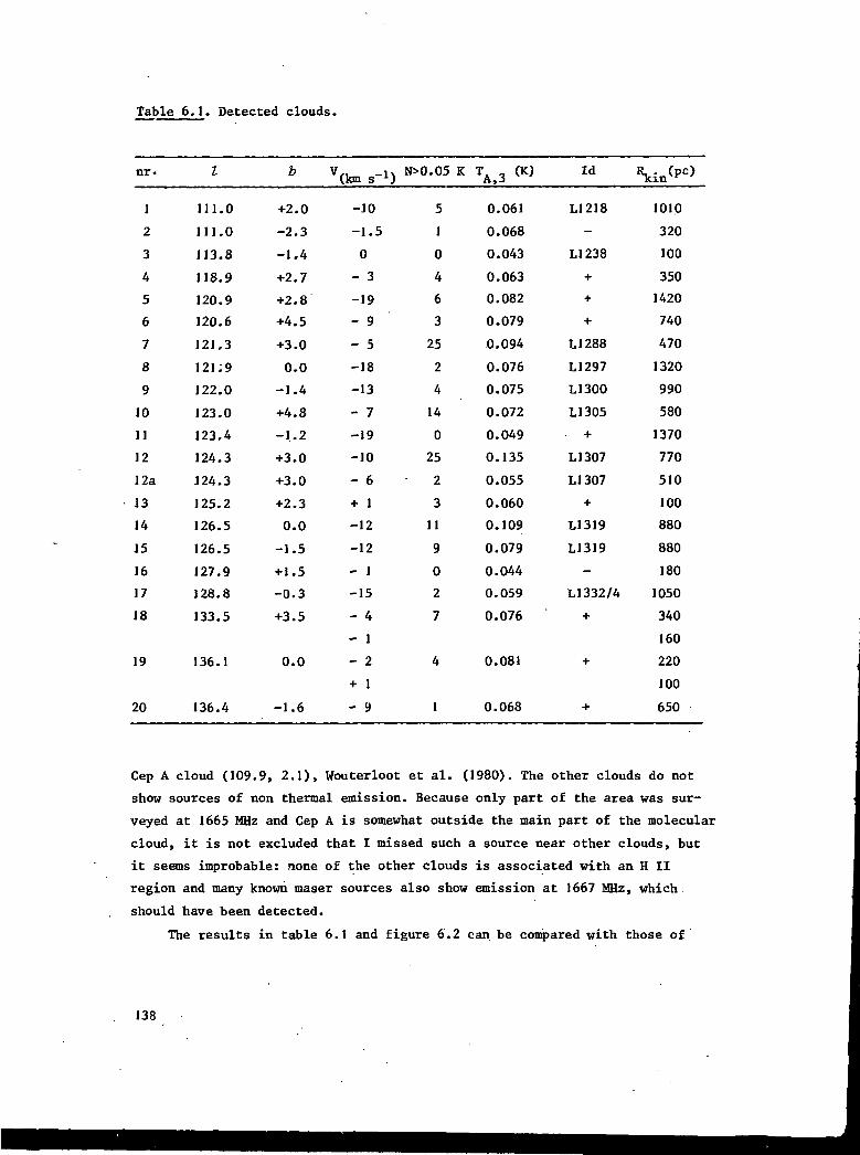
Table 6.1. Detected clouds.

nr-

1

2

3

4

5

6

7

8

9

10

11

12

12a

13

14

15

16

17

18

19

20

l

111.0

111.0

113.8

118.9

120.9

120.6

121.3

121.9

122.0

123.0

123.4

124.3

124.3

125.2

126.5

126.5

127.9

128.8

133.5

136.1

136.4

b

+2.0

-2.3

-1.4+2.7

+2.8

+4.5

+3.0

0.0

-1.4

+4.8

-1..2

+3.0

+3.0

+2.3

0.0

-1.5

+ 1.5

-0.3

+3.5

0.0

-1.6

V(km s-l]

-J0

-1.5

0

- 3

-19

- 9

- 5

-18

-13

- 7

-19

-10

- 6

+ 1

-12

-12

- 1

-15

- 4

- 1

- 2

+ 1

- 9

N>0.05 K

5

1

0

4

6

3

25

2

4

14

0

25

2

3

11

9

0

2

7

4

1

A,3

0.061

0.068

0.043

0.063

0.082

0.079

0.094

0.076

0.075

0.072

0.049

0.135

0.055

0.060

0.109

0.079

0.044

0.059

0.076

0.081

0.068

ld

LI 218

-

LI 238

+

+

+

LI 288

LI 297

L1300

L1305

• +

LI 307

LI 307

+

L1319

L1319

-

LI 332/4

+

+

+

\in (P c )

1010

320

100

350

1420

740

470

1320

990

580

1370

770

510

100

880

880

180

1050

340

160

220

100

650

Cep A cloud (109.9, 2.1), Wouterloot et al. (1980). The other clouds do not

show sources of non thermal emission. Because only part of the area was sur-

veyed at 1665 MHz and Cep A is somewhat outside the main part of the molecular

cloud, it is not excluded that I missed such a source near other clouds, but

it seems improbable: none of the other clouds is associated with an H II

region and many known maser sources also show emission at 1667 MHz, which

should have been detected.

The results in table 6.1 and figure 6.2 can. be compared with those of

138

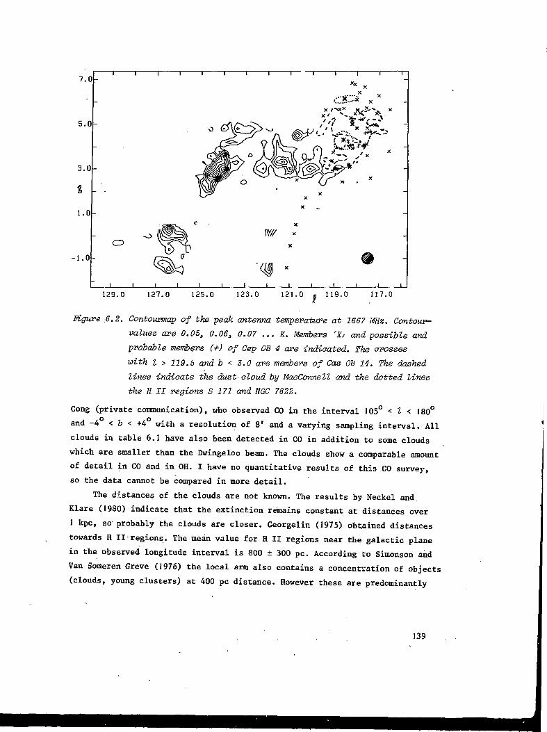
7.0

5.0

3.0

I

1.0

-1.0

J I I I I I [_ _l I I 1_129.0 127.0 125.0 123.0 121.0 n 119.0 117.0

Figure 6.2. Contourmap of the peak antenna temperature at 1667 MHz. Contour-

values are 0.05, 0.06, 0.07 ... K. Members 'XJ and possible and

probable members (+) of Cep OB 4 are indicated. The crosses

with I > 119.S and b < 3.0 are members of Cos OB 14. The dashed

lines indicate the dust cloud by MacConnell and the dotted lines

the H. II regions S 171 and NGC 7822.

Cong (private communication), who observed CO in the interval 105° < I < 180°

and -4 < b < +4 with a resolution of 8' and a varying sampling interval. All

clouds in table 6.1 have also been detected in CO in addition to some clouds

which are smaller than the Dwingeloo beam. The clouds show a comparable amount

of detail in CO and in OH. I have no quantitative results of this CO survey,

so the data cannot be compared in more detail.

The distances of the clouds are not known. The results by Neckel and

Klare (1980) indicate that the extinction remains constant at distances over

1 kpc, so probably the clouds are closer. Georgelin (1975) obtained distances

towards H II regions. The mean value for H II regions near the galactic plane

in the observed longitude interval is 800 ± 300 pc. According to Simonson and

Van Someren Greve (1976) the local arm also contains a concentration of objects

(clouds, young clusters) at 400 pc distance. However these are predominantly

139

at higher longitudes (about +10 ). The radial velocity has been determined for

some H II regions. The mean value is almost equal (within I km s"1) to that

of the OH clouds, but this is not very significant. In the following discus-

sion I shall adopt two distances for each cloud. First a kinematic distance,

using the Schmidt (1965) rotation curve of the Galaxy (listed in column 8 of

table 6.1). There exists some doubt about the continuation of the rotation

curve outside the solar circle (Georgelin, 1975; Blitz, 1979). If it is flat

at larger distances from the galactic center, the Schmidt model gives a lower

limit. However because the peculiar motions of the clouds can be relatively

large, the distances are very uncertain. Second I shall use for all clouds a

distance of 800 pc, the mean distance of the H II regions. If the radial velo-

cities have some relation with the distance, one would expect that larger

(angular size) clouds have on the' average a lower radial velocity. This is not

the case.

Only very little of the H II regions are situated in the surveyed lati-

tude interval. Only one of them is certainly associated with a detected cloud.

This is S 155 near Cep OB 3. Three other H II regions S 135, S 144 and S 154

show no OH emission in their neighbourhood. The relation of S 171 to the mole-

cular clouds will be discussed in section 6.7.

6.5. The velocity structure.

Figure 6.3 shows the emission in the central part of the observed area

it velocities between -3 and -12 km s-i. Some emission occurs at velocities

outside this interval. The velocity structure of most clouds in this figure

is very simple at the present resolution. With the exception of cloud 14, none

of the clouds show velocity gradients. Within this cloud the highest veloci-

ties are at the highest longitudes. The same occurs in cloud 5: the velocity

changes from -20 km s"1 at I = 120° to -J7.5 km s"1 at I = 121°. In general

the clouds do not show emission at different velocities at the same positions.

There are three exceptions: cloud 12, 18 and 19. For the first cloud this

second component may be a continuation of the nearby cloud 7. The components

of clouds 18 and 19 are very weak so it is not possible to draw conclusions

from their distributions.

Figure 6.4 shows a longitude-velocity diagram of the whole area dis-

playing (at each longitude) the peak intensity at intervals of 1 km s"1 in

140

5.0

3.0

1.0

- 1 .0 -

1 1 1 T"

- 3 . 0 KM/S -U .0 KM/S

5 .

3 .

l . C

- 1 . 0

5.0

3.0

1.0

- 1 . 0

5.0

3.0

1.0

-1 .0

5.0

3.0

1.0

-1 .0

-\ 1 1

- 5 . 0 KM/S

H h

-7:0 KH/S' f Sc

A h H — 1 f-

- 9 . 0 KM/S

- 1 1 . 0 KM/5

- 6 . 0 KM/5

-H 1 1 1 h

-8.0 KM/5

H 1 1 1-

-10.0 KM/S

H —t-

-12 .0 KM/S

129.0 125.0 121.0 129.0 125.0 121.0

Figure 6.3. Gontouxmaps of the emission at 1667 MHz at constant velocities-1be'tueen -3 and -12 ten s . Contourvalues are 0.04, 0.0S3 0.06 ..K.

141

136.0

134.0

129.0

127.0

I

125.0

123 .0

121.0

119.0

117.0

113.0

111.0

-i 1 1 1 1 1 1 r

_| I I I L I ! L

O

_J I I 1

J I L_ I I L_5.0 -3.0 -11.0 -19.0

V km/s

Figure 6.4. Longitude-veloaity diagram, of all clouds, ivres-peative of lati-

tude. Contourvalues are. 0.04, 0.05, 0.06, ... K.

142

the observed latitude interval. If one tries to relate this diagram to the

structure of the local arm one has to remember that only a very small part (in

longitude and latitude) of this arm was observed. The strong emission at

I = 110° is due to the Cep A OH maser source. The accompanying Cep OB 3 cloud

is only barely visible. The most striking in figure 6.4 is the apparent velo-

city gradient from -5 to -12 km s"1 between I = 120 and I = 127 . However

this feature consists of clouds at different latitudes. Cohen et al. (1980)

observed this area in CO. In a similar diagram they find an indication of two

parallel strings of clouds, with a velocity difference between 13 and 8 km s"1.

The string at the most negative velocity would represent the local spiral arm

and the other one would correspond with the expanding ring, detected in H I

by Lindblad (1967). In figure 6.4 this is not so very clear, although most OH

clouds have also been detected in CO. The diagram by Cohen et al. also shows

the earlier mentioned velocity gradient, which apparently causes a transit

from the one string into the other. I think the separation in two features is

not very well established, although Liszt et al. (1981) have an indication

for these strings at a much higher longitude. One reason is that a single

local molecular cloud has an elongated structure in this kind of l-V plots

due to the small linewidth. If there are only two clouds in each given longi-

tude interval one soon obtains the impression of two parallel strings. The

structure of these diagrams can easily be explained by a single feature with

a dispersion of 6 km s"1. Clearly this is not the most suitable region of the

galactic plane to draw conclusions about the structure of the local arm, since

both Lindblad's feature A and the expected double sine for galactic rotation

have a minimum velocity in this part of the plane. One has to take account of

a much larger area in longitude and latitude. Important data to separate the

two features can be obtained in the fourth galactic quadrant where Lindblad's

ring is expected at positive velocities and the rest of the local arm at nega-

tive velocities. Further one has to consider distances of related objects

that have been obtained through a not-kinematical method instead of only the

velocity information as often had been done.

6.6. The masses of the clouds.

Since the distances of most clouds are unknown, their masses can only

very roughly be estimated. In this section I shall use two methods. First I

143

adopt a kinematical distance which is a lower limit if the rotation curve is

flat. I assume a distance of J00 pc if the cloud velocities are positive.

Second I assume a distance of 800 pc for all clouds. Because no satellite line

data are available I can only derive optical depths via the analysis of the

average main line ratios.

The main results of the analysis are shown in table 6.2. R and R are the

mean values of respectively T 3 / ^ 2 a n d I3^I2" F o r s o m e c]Louds it was not

possible to estimate these numbers because the lines are too weak. In those

cases I adopt x. = 0 and AV = 2 km s"1. The masses are calculated using all

positions where T. , >.0.05 K except for the clouds where this value is not

reached. For clouds where x. ~ 0 I estimate if possible an upper limit of T«.

The background temperature is 3.85 K in this region and if T, « 0 I adopt

T . = 5.5 K. The mass in column 7 of table 6.2 is calculated by assuming

that the cloud has a distance of 800 pc and the value in column 8 is the mass

at the kinematical distance. The uncertainties in column 7 are due to the un-

certainty in T~. The relative uncertainties in columns 6, 8, JJ and 12 are

the same as those in column 7. N_„ in column 7 is the columndensity in the

cloud center and is derived for F = 1.0. In column 9 and 10 I give the average

width of the clouds for the two distances (the clouds can have an axial ratio

of two). The corresponding mean densities are listed in column 11 and 12.

Most of the clouds in this region«have a small optical depth and even for

those with x. > 0 ij: is probably less than 1.0. The line ratio agrees in two

cases with the results of some high resolution observations with the Effels-

berg telescope. The increase in peak antenna temperature for these observations

relative to the Dwingeloo observations is about a factor two for cloud 12:

T. _ = 0.27 K. T. , is fairly constant at the 5 observed positions with a

spacing of 7.5 arcmin., except at one position where it is 0.1 K higher. This

indicates that the filling factor for the Dwingeloo beam is probably in the

order of 0.5 as is frequently derived for local molecular clouds. The line-

width is about 2.2 km s~l, somewhat less than in Dwingeloo. This can be caused

by small systematic or turbulent motions. The same conclusions result from one

observations of cloud 8 in Effelsberg in front of a more distant cloud. The

obtained mean densities are not different from typical values in other clouds.

They vary between about 80 and a few hundred with the exception of some clouds

where the low distance limit of 100 pc was used. This distance is probably too

low because none of the clouds appears as high opacity object at FOSS prints.

144

Table 6.2. Derived parameters for the clouds in table 6.1.

nr.

1

2

3

4

5

6

7

8

9

10

11

12

12a

13

14

15

16

17

18

19

20

R

2.0 ±0.30

-

-

1.99±0.30

2.59±0.80

1.82±0.20

1.9910.30

1.60±0.10

2.92±f.5O

1.79+0.50*

1.6610.40

-

-

2.3110.60

2.3110.60

-

2.0610.30

2.30+0.50

1.6010.20

-

1

1

2

1

1

3

1

1

1

1

RI

-

-

-

.8210.

.8210.

.37±O.

.82+0.

.55+0.

•05±l.

.3810.

-

.5810.

-

-

.8010.

.80+0.

-

-

-

-

-

40

30

50

40

20

50

25

20

40

40

AVkm s"-1

2.5

2

2

3.1

2.6

2.5

3.1

2.0

2.5

3.2

2

3.1

2

2

3.1

3.1

2

3.2

2.5

2.1

2

0

0

0

0

0.

0

0.

0

0.

0

0

0

0

0

0

0

0.

0

T3

0

0

0

(+0.

(+0.

(+0.

(+0.

6+0.

(+0.,+2-0.

6-o'

(+0.

(+0.

6±0.

7)

4)

1)

7)

3

6)

6

36

7)

7)

.4

N0H_

1.6

1.4

0.9

2.0

2.2

2.1

3.0

10.7

2.0

17.0

1.0

17.2

1.1

1.3

3.5

2.6

0.9

2.0

2.0

11.2

1.4

^8002 xlOOO Ua >

1.7

0.4

0.5

2.6(+8.0)

2.9(+5.0)

1.4(+0.6)

13 (+33)

3.3+1.3

1.8(+5.0)

27115

0.8

38118

0.6

1.3

6.5(+l.3)

4.8(+l.3)

0.3

1.0

3.1

5.1+2.6

0.6

2.7

0.06

0.07

0.5

9.2

1.2

4.5

5.4

2.8

14

2.4

35

0.3

0.03

7.8

5.8

0.01

1.8

0.3

0.2

0.4

r800pc

5.6-

2.8

4.5

9.5

6.7

12.4

13.4

2.5

11.2

2.8

14.0

2.8

2.8

11.2

8.4

2.8

3.4

5.6

5.6

2.8

rkin

7.

0.

2.

16.

6.

7.

22.

3.

8.

4,

13,

1,

0,

12

9

0

4

1

1

2

1

4

0

,5

2

,3

,1

,5

,1

.8

,5

.8

.4

.3

.2

.6

.5

.8

.1

.3

n H 2

cm"3

80

-

90

120

60

80

70

130

190

240

100

190

110

120

80

80

90

160

100

320

130

2 kincm"3

60

-

600

270

30

90

110

80

150

330

60

200

160

870

80

80

400

120

300

1600

160

Ln

With the present data it is possible to make a rough estimate of the

distribution of cloud sizes and masses. Recently Liszt et al. (1981) derived

from 13C0 observations along the galactic plane between Z = 34 and 40 a size

distribution with bin sizes of 7 pc. It showed a peak at about 20 pc and a

mean value of 26 pc. The combination of distance and beamsize caused a rapid

decrease below 15 pc. Above 50 pc the results by Liszt et al. indicate a

steepening. The present observations indicate that the number of small clouds

is still rising below 10 pc with about the same slope as between 20 and 50 pc.

The size distribution does not change much for the two distance estimates. The

beam is 0.9 and 7 pc at 100 and 800 pc distance. This causes the missing of

small clouds. The CO observations by Cong made with 8' beam and a variable

grid indicate the presence of such smaller clouds. However due to the incom-

plete sampling the derivation of a size distribution is difficult. Some statis-

tical work has been done on small diffuse clouds (e.g. Knude, 1978). It shows

an increase down to two parsec. The numbers are not well comparable with those

detected in OH and CO because of the different character of the clouds. The

mass distribution shows for M„__ a slope a = d log N/d log M - ̂ 0.7 between

Ï00 and 3000 M . This number changes to about a = -J.0 for M. . . These are

upper limits of a because at larger distance the number of low mass clouds is

under-estimated. The slope can be compared with values of a = -].4 (Knude,

1978) and a = -1.7 (Liszt et al. 198J). The three numbers can be intrinsically

different because they are obtained in different size intervals, in an other

part of the Galaxy or from a different type of clouds. The values of a are

reasonably close to the value of -1.5 which Kwan (1979) predicts on the basis

of coagulation models, but I do not think that this is significant.

6.7. The relation of the clouds with OB associations.

The studied longitude interval contains four local arm OB associations:

Cep 0B 2, Cep 0B 3, Cep 0B 4 and Cas 0B 14.

Cep 0B 2 is situated between I = 95° and 106°, b = 2° and 8° at a distan-

ce of about 850 pc. It is outside the upper latitude limit of the survey. Near

the galactic plane no extended emission was found. Simonson and Van Someren

Greve (1976) detected H I at a higher latitude which is probably related to

this association.

146

Cep OB 3 at (110°, +3°) was extensively studied by Sargent (1979). She

found a CO cloud with a mass of 5000 M,_, corresponding to cloud 1 in table 6.1.Ö

It is a relatively small cloud which is elongated along the galactic plane

(mean width - 0.4). This probably is the reason why it was only partially de-

tected with the large OH beam. The mass derived from the OH observations,

1700 M- is not very far off from the mass derived from CO. Since the discovery

of the Cep A OH maser source in 1978, this source has been observed several

times in order to check its suspected variability. No meaningful variations

have been found.

The third OB association is Cep OB 4 at (118 , +5 ) near the H II regions

S 171 or W 1 (118?6, +4?3) and NGC 7822 (118?6, +6?2). OH was first detected

in absorption against W 1 by Goss (1968) at velocities of -7.6 and -13.8

km s"1. Winnberg and Lundahl (1970) tried to detect OH in this region, but no

emission was found (upper limit 0.4 K). CO was detected at one position at

-12 km s"1 (Wilson et al., 1974). Some CO observations of a small dark cloud

at the edge of NGC 7822 were made by Elmegreen et al. (1978). An extensive

ctudy of the association has been made by MacConnell (1968). He distinguishes

47 members and 25 probable and possible members. Some of these appear as

emission line stars in the catalogue of Herbig and Rao (1974). The distance to

the association is about 850 pc andMacConnell derived an upper limit for its

age of about 2 x ]06 yr. The radial velocity of the association is not known:

no members appear in the list by Abt and Biggs (J972). Three of the stars

have been observed spectroscopically by Munch (1964). The radial velocity of

one of the stars is -9.4 km s"1. Munch detected CN at a mean velocity of

-8.6 km s"1, which is the same velocity as Dieter (1967) found for the H II

region S 171. These data suggest that a cloud at about -9 km s"1 is associated

with the stars, whereas one at -14 km s"1 is in front of the stars. Similar

evidence has been found by Gragzeck (1980) and Rossano et al. (1980) respect-

ively from 21 cm H I and from recombination line measurements. Their conclu-

sion is that Cep OB 4 is surrounded by a shell, expanding at a velocity of

about 5 km s"1. MacConnell has outlined a dust cloud associated with S 171.

It has an overall size of 3 x 1.5, but contains narrower parts. He derived

from starcounts a distance to this cloud between 800 and 1000 pc and a mean

extinction of 1.4 magnitudes. From colour excesses of stars behind and beside

the cloud he obtained an average value of 2.1 magnitudes for the extinction.

Figure 6.2 shows the positions of Cep OB 4 members, S 171, NGC 7822 and of

MacConnells dust cloud with respect to the molecular clouds. Most of the

147

stars, NGC 7822 and a part of the dust cloud are outside the observed area.

No emission was detected from the dust cloud or near S 171. In other complexes

the mean distance between the centers of the association and of the molecular

cloud can be quite large (up to 60 pc in Mon OB 2 and Ori OB 1). Also the

difference in radial velocity between clouds and association can be large (up

to 10 km s"1). If these numbers (60 pc and 10 km s"1) are adopted, then the

clouds 4, 5, 6 and 7 in table 6.1 might be related to Cep OB 4. However in

most local complexes the difference between the centers of association and

clouds is half or less of the extent of the association (see chapter 8). If

this is applied to Cep OB 4, then none of the clouds 4 to 7 is close enough.

A relation would have been exceptional because the H II region is not connec-

ted to the clouds. It might be possible that an eventually related complex is

at a lower longitude or a higher latitude than the association, where no OH

observations have been made. But since these areas do not contain CO clouds

or no clouds in the Lynds catalogue, I think this is not very probable. An

explanation for the absence of a large cloud complex near Cep OB 4 is that the

formation of the association has consumed the whole complex with the exception

of some small fragments that still are present near the H II regions. But also

a tangential velocity of 10 km s"1 of (one of) the clouds 4 to 7 with respect

to Cep 0B •» could explain the absence of a cloud complex close to this associ-

ation.

One other association in this region is Cas 0B 14 at a distance of 1100

pc (Ruprecht, 1966). This association, at (I20?7, +0?8) has only 8 known

members and is not well studied. The members are indicated in figure 6.2. The

mean radial velocity of three of the stars is -4 ± 10 km s"1. Nearby molecular

clouds are the numbers 5, 7 and 8 in table 6.1. On the basis of the velocities

a relation between the association and cloud 5 or 8 is less probable. For

cloud 7 a relation is possible, but some further study (e.g. of the distance

of the cloud) is necessary to confirm this.

6.8. Conclusions.

An OH survey was made of an area of 160 square near the galactic plane

between I = 100 and I = 140 . Twenty molecular clouds with sizes between 1

and about 25 pc were detected. The masses of the clouds are between 100 and a

148

few times 101* solar masses. The results indicate that the number of small

clouds still rises until below 5 pc. The clouds with a size of 20 to 30 pc

are not related to H II regions or associations and comparable in size with

the Taurus complex. Until the distances are better determined, a comparison

has to be superficial, but it makes it probable that the Galaxy contains more

of such complexes that are not forming massive stars. Because only a small

part of the local spiral arm was observed the radial velocity distribution

gives not much insight into the structure of this arm. The distribution in

two parallel strings of clouds with a different radial velocity as was found

in CO is not confirmed. The H II region S 171 and the Cep OB 4 association

probably are not related to the detected clouds.

References.

Abt, H.A., Biggs, E.S., 1972, Bibliography of stellar radial velocities, Kitt

Peak Nat. Obs.

Blitz, L., 1978, thesis, Columbia University.

Blitz, L., 1978, Astrophys. J. 23J[, L 115.

Cohen, R.S., Cong, H., Dame, T.M., Thaddeus, P., 1980, Astrophys. J. 239, L 53.

Crutcher, R.M., J973, Astrophys. J. 185, 875.

Dieter, N.H., Astrophys. J. 150, 435.

Dieter, N.H., 1973, Astrophys. J. JJJ3, 449.

Elmegreen, B.G., Dickinson, D.E., Lada, C.J., 1978, Astrophys. J. 220, 853.

Georgelin, Y.M., J975, thesis, Universitë de Provence.

Goss, W.M., 1968, Astrophys. J. Supp. J5., 131.

Grayzeck, E.J., 1981, Astron. J. J35, 1631.

Herbig, G.H., Rao, N.H., 1972, Astrophys. J. 174, 401.

Humphreys, R.M., 1980, in: The large scale characteristics of the galaxy, ed.

W.B. Burton, p. 93.

Khavtassi, J., 1960, Atlas of Galactic Dark Nebulae, Tiblisi, Abastumani Astro-

phys . Obs.

Knude, J., 1978, Astron. Astrophys. Supp. 33_, 347,

Kwan, J., 1979, Astrophys. J. 229, 567.

Lindblad, P.O., 1967, Bull. Astr. Inst. Neth. 1J>, 34.

Lindblad, P.O., Grape, K., Sandqvist, Aa., Schober, J., 1973, Astron. Astro-

phys. ̂ 4 , 309.

Liszt, H.S., Burton, W.B., Bania, J.M., 1981, Astrophys, J. 246, 74.

149

Lynds, B.T., J962, Astrophys. J. Supp. T_, 1.

MacConnell, D.J., 1968, Astrophys. J. Supp. J£, 275.

Minn, J.K., Greenberg, J.M., 1973* Astron. Astrophys. 22_, 13.

Münch, G., 1964, Astrophys. J. 140, 107.

Neckel, Th., Klare, G., 1980, Astron. Astrophys. Supp. 42_, 251.

Rossano, G., Angerhofer, P., Grayzeek, E.J., 1980, Astron. J. 85, 716.

Ruprecht, J., 1966, Trans. I.A.U., J2B, 350.

Sargent, A.I., 1979, Astrophys. J. 233, 163.

Schmidt, M., 1965, in Stars and Stellar Systems V, ed. A. Blaauw.

Simonson III,S.C., Van Someren Greve, H.W., 1976, Astron. Astrophys. 49_, 343.

Wilson, W.J., Schwartz, P.R., Epstein, E.E., Johnson, W.A., Etcheveriy, R.D.,

Mori, T.T., Berry, C.G., Dyson, H.B., 1974, Astrophys. J. 191, ̂ 57.

Winnberg, A., Lundahl, L., 1970, Astron. Astrophys. 2> 3 2 1•

Wouterloot, J.G.A., Habing, H.J., Herman, J., 1980, Astron. Astrophys. _8^, Lll.

150

CHAPTER VII

MOLECULAR CLOUDS IN THE PERSEUS ARM

7.1. Abstract.

In this chapter I present OH observations of molecular clouds made to

study the structure of (a part of) the Perseus spiral arm. First I searched

approximately 160 square degrees for OH clouds with the 25 m Dwingeloo tele-

scope. Next the detected OH clouds were studied in more detail with the 100 m

Effelsberg telescope together with ?. number of clouds, missed in Dwingeloo

but detected during a CO survey of the same area by Cong.

After an introduction in section 7.2, the methods of the observations

are described in section 7.3. The results of the OH observations are described

and analysed as far as the individual clouds are concerned in section .7.4.

In section 7.5 I first give a discussion of the properties of the OH clouds

in relation with other spiral arm tracers and then a general picture of the

structure of the Perseus arm.

7.2. Introduction.

Whether there is.a relation between molecular clouds and spiral struc-

ture in our Galaxy is not yet well known. I already mentioned in chapter 1

that poorly sampled surveys in the first galactic quadrant do not reveal an

ordering of CO in spiral arms. In a survey in the first and second quadrant

by Cohen et al. (1980), a coincidence of CO and H I features appeared to be

present. Liszt and Burton (1981) however showed for the second quadrant that

this coincidence can be caused by kinematic effects alone and that a large

density enhancement in the spiral arms is not needed. Due to the large

distances, involved the observations by Cohen et al. in the first quadrant

tell little about the possible distribution of molecular clouds within the

large scale structure of a spiral arm. ,

151

Clear examples of large scale spiral structure can of course be found in

other galaxies. The Hubble type of the Galaxy is between Sb and Sc (Georgelin,

1975) and it has probably four main spiral arms and r~Moe spurs in between. In

galaxies of nearly the same type the thickness of the arms is between 400

(M 101) and 900 pc (H 100). Some galaxies show strings (100 to 300 pc in size)

of many H II regions at regular distances (1 to 2 kpc) in the outer parts (e.g.

M 101). Many galaxies show dust lanes at the inner side of the spiral arms,

but in some galaxies these are partly within an arm. Molecules have been ob-

served in external galaxies (Rickard, 3979), but most observations were made

in the nuclear region. Only in M 31 CO has been detected in the dust lanes of

the outer arms, but the interpretation of these observations is still under

discussion (see e.g. Rickard, 1979; Stark, 1980).

A spiral arm in our Galaxy, suitably located to study its structure, is

the Perseus arm and so many studies of this arm have been made. The advantages

of this choice are the following. The distance of the arm is reasonably small,

the arm is outside the solar circle and a large part of it is viewed under a

very favourable angle. No other (major) arms are seen projected against the

Perseus arm, and most objects in it can be seen individually without super-

positions. The Perseus arm has also some disadvantages: the rotational velo-

city outside the solar circle is not very well known and kinematical distances

are unreliable. The arm is located at a large distance from the galactic cen-

ter where the shock, expected from the density wave theory is weaker than in

the inner arms. This will probably decrease the star or cloud formation rate

and may therefore have arofound effects on the arm as a whole; in other words:

the arm may not be typical for all spiral arms.

The Perseus arm was studied extensively by many authors. I will give here

a short summary.

The neutral hydrogen distribution was discussed among others by Weaver (1974),

Verschuur (1973) and Rohlfs (1974). Generally it is found that the H I kine-

matics does not coincide with that of the optical arm, the H I having more

negative velocities. From an analysis of the H I- gas at higher latitudes

Verschuur concluded that there is probably another minor spiral arm behind the

Perseus arm which he called the a-arm. Absorption and emission studies in the

21 cm line have been made with high angular resolution of several objects

(e.g. NGC 7538, Read, 1980). These measurements allow more detailed discussi-

ons of the gas in front of these objects and of H I clouds associated with

the molecular clouds.

152

H II regions and stellar associations. Georgelin and Georgelin (1976) and

Crampton et al. (1978) discuss the distribution of H II regions. They find a

general distance of about 2.5 to 3 kpc to the arm, but a number of objects are

at 5 to 6 kpc, which possibly indicates the existence of another arm. Some in-

dividual H II regions have been studied by Israel (1976). A radio continuum

survey at 21 cm of this area was recently made by Kallas and Reich (1980).

This survey can be used to obtain statistical information about the properties

of H II regions in different parts of the arm. A similar survey was made by

Price (1981) in the far infrared. Humphreys (1976) studied the velocity dis-

tribution of associations, clusters and H II regions and finds possible stream-

ing motions. The distribution of high luminosity stars in a number of fields

is discussed by Wramdemark (1976, 1981) and Martin (1972). They find a strong

maximum in the numbers of stars at a distance around 3 kpc. Munch (1957) de-

tected interstellar absorption lines in front of the associations with a more

negative radial velocity than the emitting stars. The Perseus arm area con-

tains several supernova remnants. The distance of these objects cannot be

derived very precisely. Braunsfurth et al. (1979) obtained radial velocities

of three of them through their influence on the H I. They agree with the

stellar radial velocities which makes the association quite probable.

Kinematiaal models of the Perseus arm have been made by several authors. I

mention here Burton and Bania (1974), who madr» correlations of H I and optical

spiral arm tracers as a function of different perturbations of the Schmidt

rotation model. Roberts (1972) made a model of the arm involving a Galactic

spiral shock that explained all observational results known at that time.

Molecules have been observed in the vicinity of several H II regions,

e.g. near NGC 7538 (Minn and Greenberg, 1975), S 156 (Hogland and Gordon,

1973) and W3 (Lada et al., 1978) some of which show the presence of an H20 or

OH maser. To study the distribution of molecular clouds in a spiral arm and

their relation with other objects I have carried out the observations de-

scribed in this chapter. I first made a survey of large OH clouds with the

Dwingeloo telescope and I followed this up by making detailed maps of the

detected clouds with the Effelsberg telescope. Also at Effelsberg I obtained

OH data on a number of CO clouds observed in a CO survey by Cong (private

communication).

A schematic overview of all objects within the Perseus arm between I = 100°

and Z = 140 is given in section 7.5, in figure 7.9.

153

7.3. The observations.

The Dwingeloo observations (beamsize 31', beam efficiency 0.76) were made

in 1978 at a grid of positions, 0.3 apart in galactic longitude and latitude.

The area extents from Z = 100° to 139° and is irregular in latitude (on the

average from -1?7 to +2?5, see figure 6.1). It covers 163 square degrees. The

latitude extent was chosen to include as much as possible H II regions which

are situated in the Perseus arm. The observations were made at 1667 MHz with

a resolution of 0.9 km s"1 and an integration time of 30 minutes. This re-

sulted in noise with an r.m.s. value of about 0.02 K. A part of the observa-

tions was made in the more sensitive 2 bit correlator mode. The observations

were made in the total power mode with reference measurements of about two

hours taken at the North Pole every 12 hours. Because molecular clouds are ex-

tended and posses a range in brightness temperature, it is not possible to

make accurate estimates of the completeness of the survey. I estimate that

most, say 90% of the clouds with sizes above 25 pc and a mean brightness

temperature T_ > 0.2 K have been found. This fraction decreases for lower size

and Tn.a

Five clouds were detected in Dwingeloo and in May and June 1979 they were

observed in Effelsberg (beamsize 7l8, beam efficiency 0.70) at a 7.5 grid.

These observations, made with a resolution of 1.1 km s"1 and an integration

time of 30 minutes, were started at the Dwingeloo cloud center and moved out-

ward until the cloud boundaries were reached. I used the frequency switching

mode with the signal appearing in both bands. The two main lilies were observed

simultaneously. A second set of observations at Effelsberg concerned the CO

clouds discovered by Cong with the New York telescope and made available to

me. The same resolution and integration time was.used to observe the centers

of these clouds. At some positions with a high antenna temperature I made

additional observations at Effelsberg with a higher resolution (0.3 or 0.6

km s"1) to see if the line has more components. Some other positions were

observed with a longer integration time to improve the signal to noise ratio.

During a test of the system at 1720 MHz I made an observation with a resolu-

tion of 0.07 km s"1 (integration time 5 minutes) of the NGC 7538 1720 MHz

maser. Left and right circular polarisation were observed simultaneously.

During the observations in Effelsberg the two channels of the receiver system

were saturated unequally. This (slightly time dependent) effect was noted

154

too late and could not be corrected for fully. The remaining uncertainties of

the relative intensities of the two lines are about 5 percent. The corrections

to the absolute intensities could amount to a factor 2.

7.4. The observational results.

7.4.1. Dwingeloo.

The results of the Dwingeloo observations can be split into two parts,

considering the radial velocity of the detected clouds. First I found several

clouds with V > -20 km s"1, which are probably related to the local spiral

arm. They have been discussed in chapter 6. Second I found a few clouds with

V < -45 km s"1 belonging to the Perseus arm. The Dwingeloo beam of 0.5, the

0?3 grid and the sensitivity will only select large molecular clouds with

sizes in both directions of 25 pc or more. Clouds were considered real if they

have peak intensities above 0.08 K and are detected at at least two adjacent

positions. Weaker features or signals appearing at only one position, were

remeasured for confirmation, however without succes. The observed part of the

Perseus arm (163 square degrees or 0.45 kpc2 at 3 kpc distance) appears to

contain 5 large clouds. They are listed in table 7.1. Since all of them have

been mapped at Effelsberg I will not present the Dwingeloo maps of the clouds.

The number of positions with T. _ > 0.06 K in column 4 of table 7.1 indicatesA, o

the size of the cloud. Column- 5 gives the highest antenna temperatures T. ,A, J

measured in Dwingeloo. Note that the values of T. , are all higher than theA, J

peak value of the Rosette cloud (chapter 3), so clouds of that nature will

already have been missed.

Table 7.1. Clouds detected in Dwingeloo.

V

104.8

108.7

110.0

111.5

132.8

b

0.3

0.3

-0.3

0.6

0.9

V

-55.0

-54.2

-51.2

-53.6

-43.0

N

3

4

5

7

3

TA, 3

0.09

0.10

0.13

0.10

0.12

rel.

S

S

W

ob j.

-

-

146

158

3

155

0.50 -

Q25

Figure 7.1.

1667 MHz map of aloud 104.8 + 0.3. Contourvalues are 0.07 and 0.10 K.

105.0 104.5

7.4.2. Effelsberg observations of Dwingeloo clouds.

I will first discuss individually each of the five clouds which have

been mapped with the Effelsberg telescope and next those for which I have only

one detection at a single position. I will not use kinematical distances but

adopt a distance of 3.5 kpc unless more specific information is available. For

the first three clouds I will show only the 1667 MHz maps. Those at 1665 MHz

are similar but the signals are too weak to get a reliable map.

a. Cloud 104.8 + 0.3. This cloud is very isolated and not associated

with any known H II region. The peak antenna temperature in Effelsberg is

0.11 K, comparable to that in Dwingeloo. This indicates that there is not much

variation in brightness temperature over the cloud. At Effelsberg the cloud

has been detected only at a few positions. A rough contour map is shown in

figure 7.1. The radial velocity is approximately constant and equal to

-53.7 km s"1. Also the linewidth does not vary much; its mean value is 2.2

km s"1. The size of the cloud is 22 pc, for a distance of 3.5 kpc. The line

ratio cannot be obtained with sufficient accuracy and I will adopt x, = 0

T = 5.5 K as is found generally in local clouds. In that case I arriveCA) J

at a cloud mass of about 6.9 * 103 M . The cloud is outside the longitude

range, observed in the CO survey by Cong, and no additional information is

available.

b. Cloud 108.3 + 0.3. This is a somewhat larger cloud than the previous

one, but also in this cloud no details are visible. A contourmap is shown in

figure 7.2. There are two regions with a peak temperature of about 0.2 K, a

factor two higher than in Dwingeloo. One of these peaks corresponds with the

position of maximum emission in CO (Cong, private communication). The extent

of this cloud is about 30 pc. The velocity is constant at about -52.8 km s"1

and the linewidth is 2.3 + 0.9 km s"1 for both transitions. The line ratiospoint to a low Xy For 0 the mass is 1.6 x 104 M . It has been detected

156

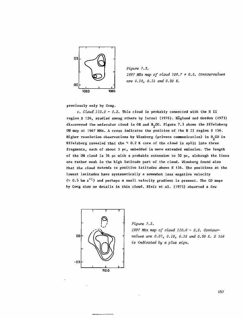
Figure 7.2.

1667 MHz map of aloud 108.7 + 0.3. Contourvalues

are 0.10, 0.15 and 0.20 K.

109.0 1085

previously only by Cong.

c. Cloud 110.0 - 0.3. This cloud is probably connected with the H II

region S 156, studied among others by Israel (1976). Höglund and Gordon (1973)

discovered the molecular cloud in OH and H 2C0. Figure 7.3 shows the Effelsberg

OH map at 1667 MHz. A cross indicates the position of the H II region S 156.

Higher resolution observations by Winnberg (private communication) in H-CO in

Effelsberg revealed that the ̂ 0.2 K core of the cloud is split into three

fragments, each of about 5 pc, embedded in more extended emission. The length

of the OH cloud is 36 pc with a probable extension to 50 pc, although the lines

are rather weak in the high latitude part of the cloud. Winnberg found also

that the cloud extends to positive latitudes above S 156. The positions at the

lowest latitudes have systematically a somewhat less negative velocity

(̂ 0.5 km s"1) and perhaps a small velocity gradient is present. The CO maps

by Cong show no details in this cloud. Blair et al. (1975) observed a few

Figure 7.3.

1667 MHz map of cloud 110.0 - 0.3. Contour-

values are 0.07, 0.10, 0.15 and 0.20 K. S 156

is indicated by a plus sign.

-0.5 -

110.0

157

112.0 111.5 111.0 112.0 111.5 mo

Figure 7.4. 1665 (left) and 1667 IWZ (right) map of aloud 111.5 + 0.6. Contour-

values are 0.073 0.10 and 0.15 K. The position of the maser sourae

is indicated by a plus sign.

positions in CO. They obtained rather high temperatures, from 10 K to 22 K

near S 156. The H II region is at a higher galactic latitude and thus it has

a somewhat unusual (projected) position with respect to the cloud. However,

the H II region may be at the front side of a cloud which is stretched out

along the line of sight. Only a minor part of the cloud is directly behind

S 156 as also che H^CO data pointed out. However this minor part is probably

enough massive to agree with the blister model by Israel. At a distance of 3.5

kpc and if T, = 0, the mass is 4.4 x \Qh M. The H„C0 observations indicatedj is Z

that the cloud probably has a low filling factor, perhaps between 0.3 and

0.5. Höglund and Gordon did not give a mass estimate.

d. Cloud 111.5 + 0.6. The area of the H II region NGC 7538 (or S 158) is

well known for the star formation that goes, on there. I will not give an ex-

tensive review of earlier observations of this region, but refer to Read

(1980) for a recent summary. The molecular cloud associated with NGC 7538 was

discovered in H2CO by Minn and Greenberg (1975). They detected three clouds,

which they called complex I to 3, with different radial velocities, at least

5 km s"1 less negative than that of the H II region. Read (1980) made aper-

ture synthesis observations of H I in absorption in front of S 158 and in

emission outside the H II region. He found that at the position of the mole-

cular cloud the H I is anticorrelated with the H-CO. This he explained by

selfabsorption. Selfabsorption is most clearly seen for the -55 km s"1 cloud

(complex 1 of Minn and Greenberg), but of the -52.5 km s"1 cloud (complex 3),

158

half of the H-CO is outside the H I distribution, which is more extended to-

ward lower latitudes.

The OH map at 1667. and 1665 MHz is shown in figure 7.4. The higher longi-

tude part of the cloud (complex 3) is more extended in OH than the other side

(complex 1). Like the H„CO, the OH complex 3 is at a higher latitude than the

corresponding H I feature. The mean OH velocities, -52.4 and -54.4 agree with

that of the H^CO. Complex 2 could not be detected in OH and its reality is

very uncertain. A clear jump in radial velocity indicates that cloud 111.5

+ 0.6 does not consist of one cloud with a velocity gradient, but of two sepa-

rate clouds as is the case in the Mon OB 1 area (chapter 3). When OH is com-

pared with H_CO one result is that the OH is more extended. An exception is

the area near S 158, where no OH could be detected, because of confusion with

the strong OH maser source at 1 = 111.475, b = 0.85 (indicated with a cross

in figure 7.4). The larger size of the OH cloud is probably not due to the

40% larger OH beam but reflects the difference in OH and H-CO abundance. Minn

and Greenberg found that the lines of the H-CO clouds are very broad (about

5 km s"1). Although the OH linewidths are not as large, they are yet larger

than in the other Perseus arm clouds, the mean value is 3 i 0.5 km s for

the two clouds. I do not find indications for a larger linewidth in the cloud

center as Minn and Greenberg did. Minn and Greenberg explain the increase in

linewidth by cloud contraction. The sizes of the two clouds are respectively

25 and 35 pc. Based on observations of other and more nearby clouds I think

that it is very unlikely that such big clouds are in a state of contraction.

The line ratio T. -,/T. o appears to be rather different for the centers

of the two complexes. In complex 1 they are about 1.0 (high optical depth)

and in the center of complex 3 they are around 2.0 (low optical depth). Also

the H I optical depth is larger than that of complex 3. However because the

line ratios cannot be estimated with sufficient accuracy I will assume T_ = 0

for both complexes. Then the masses are respectively 1.3 x 101* M (complex 1)

and 3.9 * 10 M~ (complex 3), again for a distance of 3.5 kpc. Because of

optical depth effects the mass of complex 1 may have been underestimated and

that of complex 3 somewhat overestimated.

Figure 7.5 shows the left and right circularly polarized spectra made

with high resolution (0.07 km s"1) of the 1720 MHz maser source near NGC 7538

observed at the position by Wynn-Williams et al. (1974). They and Hardebeck

(1971) previously observed the sources with low velocity resolution

(0.7 km s"1). The spectrum by Hardebeck shows that the maser has two components

159

00-

-630 -600 -570 -510kmft

Figure 7.5. Left (left) and right (right) circularly polarized spectra at

1720 MHz of the maser source near NGC 7538.

at -57.2 and -60.J km s"1. The components visible in figure 7.5 are listed in

table 7.2. The line at -59.4 km s"1 is probably unpolarized. It has linewidths

of 0.20 and 0.28 km s"1 with a possible velocity difference of 0.08 km s"1 be-

tween left and right circular polarization, which is not significant. The

other component has more structure, that is at least partly circularly polar-

ized. The left circularly polarized spectrum shows two and perhaps three com-

ponents. The right circularly polarized spectrum probably has two components,

judging from the large linewidth. The intensity scale in figure 7.5 can be

somewhat in error as was mentioned before (section 7.3). Forster et al. (1980)

have discovered an H„C0 maser near S 158. This maser source happens to have

components at almost the same velocities as the 1720 MHz OH maser, but the

positions are not the same. It probably is a chance coincidence. The two

Table 7.2. Line parameters of NGC 7538 1720 MHz maser.

Pol V km/s F Jy LW km/s

L

R

-59.39

-57.77

-57.35

-57.12

-59.31

-57.66

-57.43

19.4

23.6

16.9

24.0

17.2

17.1

21.6

6 .8

8 .3

5 .9

8 .4

6 .0

6 .0

7.6

0.27

0.35

0.30

0.30

0.21

0.30

0.30

160

groups of lines at o, -57.5 km s"1 and -59.5 km s"1 appear to originate from

different positions (Forster, private communication) but the positions of in-

dividual components are not known.

e. Cloud 132.8 + 0.9. The last Perseus arm cloud that I have mapped in OH

is the one near the W3 complex. I will not discuss all existing data about W3;

Goudis (1979) made a review. The cloud was mapped previously in CO by Lada et

al. (1978). OH was first detected in this cloud by Höglund and Andersson

(1974) at their position nr 250. They found an antenna temperature of 0.055 K

with a 29' beam. I started my OH observations at one of the CO positions of

maximum emission. In a part of the observations, usually up to distances of

30 arcmin. from W3 OH, I noticed stray radiation from this maser source through

the sidelobes of the telescope beam. Where this is recognized, the 1665 MHz

line is 10 times stronger than the 1667 MHz line and the emission is at -45

and -41.5 km s"1. At I = 133?23, b = 0?9 I find 1665 MHz emission at -44 km s"1

and near that position also emission at -41 km s , but because the J667 MHz

line is equally strong I assume that the emission is from a real cloud, but

that the 1665 MHz line perhaps has a contribution of sidelove emission of

W3 OH. Therefore I do not trust the line ratios in that area.

Maps of the 1665 and 1667 MHz peak antenna temperatures of the cloud are

shown in figure 7.6. The two maxima at 1667 MHz coincide with peaks in the

high resolution (2.3) CO map by Lada et al. (1978). This confirms that the

peaks are real. Two peaks at lower latitude in the low resolution CO map are

134.0 133.5 133.0 134.0 1335 1330

Figure 7.6. 1665 (Left) and 1667 MHz (right) map of aloud 132.8 + 0.9. Con-

tourvalues are 0.103 0.20, 0.Z03 ... K.

161

not detected in OH, probably because of a lower OH columndensity. These

peaks neither show up very clearly in the high resolution CO map. It is this

region where Hasegawa et al. (1980) find signs of H I self absorption. The

H I could not be analysed for the region where I detected OH due to confusion

with H I absorption by W3. The absence of OH in regions with H I selfabsorption

is uncommon. Other regions with H I selfabsorption do show OH, e.g. cloud 2

(chapter 5) or the P Oph cloud (chapter 4). The selfabsorption interpretation

of the H I is in this case not necessarily unique. In this complex molecular

emission is visible at velocities between -40 and -50 km s"1. If all those

clouds are associated with an H I cloud, this will cause dips in the line

profile that could be mistaken for self absorption.

I have made high velocity resolution (0.3 km s~x) observations at the two

peak positions in the OH cloud: position 1 = (132.975, 0.775), position 2 =

(133.225, 0.9). The spectra are shown in figure 7.7. The lines are well re-

solved with a total width of 2.0 km s"1 at both positions for the 1667 MHz

line. There is a weak indication that the profiles consist of components at

different velocities. However this explanation is rather unlikely because the

velocities of the apparent peaks do not agree for the two transitions. The

antenna temperature at the first position (fig. 7.7, left), 0.62 K, is very

high in view of the low resolution, 5.9 pc, and the area deserves some more

detailed observations. At a comparable resolution in the Mon OB 1 cloud

(chapter 3) I find only a peak antenna temperature of about 0.15 K. In Taurus

(resolution 1 pc), the peak T. _ is 0.35 K. At position 1 the 12C0 temperatureA, J

is not very high, between 10 and 15 K. The OH line ratio at position 1 is

about 2.0 (low OH opacity), thtt at position 2 is about 1.0 (large OH opacity).

Because the spectra were taken in succession the difference in line ratio ap-

pears to be real. (The high resolution observations do not show a component

at -45 km s"1, the velocity of the strongest W3 OH emission.) In the rest of

the cloud the line ratio is systematically higher near position 1 than near

position 2, although an accurate value cannot be determined due to the cali-

bration problems mentioned before.

I calculate the mass in two ways. Firstly I take x_ = 0 everywhere in the

cloud. Secondly I take T^ = 0 near position 1 and T. = 2 near position 2. In

those cases the total mass of the cloud is respectively 4.4 * 101* Mft and

5.6 x 104 Mrt (at 3.5 kpc distance). This is somewhat larger than Lada et al.

derive for this part, which they call "rest of the cloud" (< 3.0 * 101* M_).

However they assume a smaller distance to W3 (2 kpc), which may be more

162

030

020

030

\000

010

1665MHz -J

1A i l lM

1 M l

020 -

-5600 -1600 -4000 -3200

-010 -

-5600 -48.00 - " 0 0 - 3 i 0 °

060

0.40

020

000

1 1

I .

i i

i > i i i

. 1667MHzrt

i i i i i

030 -

-56.00 -48.00 - 4 0 0 0 km/s - 3 2 0 0

-010 -

-5600 -4800 - 4 0 0 0 kmte - 3 2 0 0

Figure 7.7. High vesolution 166S and 1667 MHz speatra at (132.975, 0.775)3

left and (133.225, 0.9), vight.

realistic. So the two results are in agreement. There may be a velocity gra-

dient in the complex, in particular in the cloud near position 1 where the

radial velocity decreases with latitude from about -42 to -44 km s"1.

7.4.3. Effelsberg observations of New York (CO) clouds.

With the J.2 ra telescope at Columbia University, New York, Cong (unpub-

lished) observed in 12C0 the Perseus arm between I = 105° and I = 140°. Cohen

et al. (1980) presented some results of this survey. From a preliminary list

I selected the CO clouds with the highest temperatures and searched for OH

with the Effelsberg telescope at the CO peak position. Of the 61 CO positions

in Congs list I observed 29 and detected 22 in at least one spectral line.

In total I have OH data of 30 clouds in the Perseus arm because cloud

163

Table

no.

1

2

3

4

5

6

7

8

9

10

11

12

13

14

15

16

17

18

19

20

21

22

23

24

25

26

27

28

29

30

7.3.

I

104

105

108

108

109

109

110

111

111

111

111

HI.

111.

112.

113.

114.

115.

117.

118.

120.

120.

123.

132.

133.

133.

133.

134.

136.

137.

138.

.7

.625

.75

.75

.0

.875

.125

.25

.25

.25

.5

.5

.625

.125

.0

.5

,75

.0

.625

,125

625

125

88

28

51

82

15

88

68

52

0

0

-1

0

-0

-1

0

-3

-1

-0

0

1,

-3.

-2.

-0.

-0.

-1.

-2.

-1.

2.

-0.

-0.

0.

0.

1.

0.

0.

1.

1.

1.

b

.3

.375

.0

.25

.25

.25

.0

.125

.5

.625

.75

.25

.5

.5

.75

.5

,625

.25

.375

,125

,375

875

79

49

0

54

81

11

52

65

TA,3

0.11

<0.06

0.11

0.15

0.1J

<0.06

0.19

0.10

<0.08

0.10

0.12

0.14

0.12

<0.05

0.15

0.09

<0.05

.0.09

0.07

0.08

0.08

0.11

0.13

0.12

0.24

0.07

0.18

<0.06

-0.30

-0.18

<0.10

-0.19

AV

2.1

2.1

2.2

3.4

2.8

4.0

1.4

3.3

3.2

1.3

1.3

2.0

4.6

5.9

3.4

4.7

2.0

2.4

2.0

2.6

3.5

2.3

3.9

2.5

1.3

V

-53.7

-51.0

-52.9

-47.6

-52.0

-43.2

-48.8

-53.4

-46.0

-42.3

-33.7

-47.7

-42.9

-40.0

-50.0

-46.7

-57.0

-44.5

-18.7

-42.4

-48.3

-43.0

-50.0

-41.5

-39.1

TA,2

0.06

<0.07

<0.07

0.07

0.09

<0.06

0.08

0.04

<0.06

<0.06

0.09

<0.06

0.10

<0.08

<0.06

0.16

<0.05

<0.08

<0.07

<0.07

<0.06

0.11

0.09

0.08

0.15

<0.06

-

-

-0.26

-0.11

<0.05

-0.09

AV

2.3

2.4

2.7

3.1

3.0

2.6

1.3

1.5

1.1

1.8

1.5

2.2

3.9

2.5

1.3

V

-53.8

-52.7

-46.7

-52.2

-43.2

-53.4

-45.2

-48.9

-57.9

-44.9

-18.4

-42.7

-50.0

-41.6

-39.1

164

104.8 + 0.3 was not observed in CO. The data are shown in table 7.3. I will

discuss individual detections only if necessary, but will concentrate on the

statistical properties.

At some positions more than one component is visible, e.g. position 22

contains also a local cloud discussed in chapter 6. Three clouds (nr. 27, 28

and 39) were detected in absorption against H II regions around W4 and W5. An

exceptional narrow absorption line is seen in front of S 201. The linewidth

probably is 0.6 to 0.7 km s"1 after deconvolution from the velocity resolution.

This is much less than seen at other positions. All line ratios point to ther-

mal emission except at one position, near the H II region S 152 (see section

7.4.4).

The CO data and other important information about the observed positions

are listed in table 7.4. In column 2 is the CO antenna temperature and in co-

lumn 3 the corresponding excitation temperature. Column 4 shows an effective

CO linewidth, obtained by dividing the integrated line intensity by the peak

antenna temperature. In column 6 is the eventually related H II region with

its radial velocity in column 7. Column 8 gives a mean diameter of the cloud,

where the CO antenna temperature is about half its peak value. This is an un-

certain value, but no more data were available. Column 9 shows the velocity

of u ximum H I emission at each position, obtained from the Maryland-Green-

bank survey (Westerhout, 1972), which was made with a 10' beam. For each

cloud I used the Maryland-Greenbank survey to make an H I latitude-velocity

diagram through the cloud center. In general the H I has its maximum intensity

at a single velocity around -50 km s"1. The H I velocity at the position of

the cloud was estimated from this diagram. If at that position the H I showed

more velocity peaks, not caused by selfabsorption, I used the one closest in

velocity to the molecular cloud. This occurred only in a few cases. Column 10

of table 7.4 gives the OH column density Nrt„. In all cases N_.„ has been calcu-

lated by assuming t = 0 because the signal to noise ratio of the 1665 MHz

line was too small to derive a better value. This means that N.„ is a lowerOn

limit. For the five clouds with a complete OH map the values are an average

for all positions where both lines were detected. To estimate the column dens-

ities at positions where I measured OH in absorption I used the continuum

observations of Wendker and Altenhoff (1977) at 11 cm and of Rohlfs et al.

(1977) at 21 cm. The background brightness temperatures are then 6.2, 6.4 and

2.3 K at the positions 27, 28 and 30 respectively. The continuum emission at

the first two positions may have a component in front of the molecular cloud,

165

Table

no.

1

2

3

4

5

6

7

8

9

10

11

12

13

14

15

16

17

18

19

20

21

22

23

24

25

26

27

28

29

30

T

3

5

7.4.

CO

.1

.01.53.04

2

6322216,

3.

I.

2.

1.

3.

4.

2.

2.

2.

1.

2 .

3 .

2 .

3 .

3.

4 .

3.

4 .

3 .

.5

. 0

. 5

.7

.5

.5

.4

.6

.5

.3

.9

.5

.3

.5

.5

.0

,6

5

,4

9

4

29

6

0

9

3

0

T

6

8467

5

965,5,5,4,9.

6.

5.

5.

4.

6.

7.

5.

5.

5.

4 .

6 .

6 .

5 .

7.

6.

7.

7.

7.

6.

ex

. 3

. 3

.6

.2

. 8

.1

.8

.9

.7

.7

.6

.7

.8

.5

.0

.7

.4

.7

.8

1

8

7

5

1

6

4

2

8

3

2

6

2

AV

5

4

(6

4

6

5

(13

9

(6

12

5

13

7

7

4

3

6.

4,

3,

7,

5.

4.

7.

5.

5.

5.

8.

4.

7.

e f f

. 4

. 8

.3 )

. 4

.5

.9

.8 )

.6

. 7 )

. 0

.5

.2

.6

.7

.9

.6

.0

.6

.6

.1

.5

,7

.7

,4

6

,5

2

4

0

vco

-52.0

-51.1-47.3-52.5-47.5

-33.0

-51.8-41.5-34.9-39.4-43.1-47.5-55.4

-46.2-45.2

-37.5

-34.5

-49.4

-39.2

-43.8

-39.1

-50.3

-46 .3

-44.5

-42

-50

- 4 3

-47

-50

-40

-39

- 3 8

H II

S138

S152.S153

S156

S157

S158

S168.S169

S172

SI 75

S177

S201

VH I I

-60.0

-44.3

-51

-46

-59

- 4 4

-50

.7

.6

. 5

.7

-51

-56

-49

-47

- 4 5

- 4 3

-47

- 4 3

- 4 7

- 4 8

-47

-

-39

I

.5

.1

.0

.5

.5

.0

.0

.0

.5

. 5

.5

.0

-49 , -40 .

- 4 6

-39

- 4 8

-40

-49

- 4 5

-41

- 4 4

- 5 4

-52

-51

-52

-50

-41.

-41.

.5

.0

.5

.0

.0

.5

.0

.0

.0

.0

.5

.0

.5

size(degrees)

0

0

0

0

.3

.5

.7

.6

0 . 5

0

0

0

0

0

1.

0.

0.

0.

5 0.

0.

0.

0.

0 .

0 .

0,

0 .

0 .

0 .

0 .

0 .

0 .

0 .

0 .

0 .

. 3

.8

.8

.5

.3

.0

.4

.4

.5

.3

.5

.4

.4

.3

,3

.3

6

4

4

4

4 •

4

3

3 •

3 .

N0H

2.1 x lO1**

<1.1

2.1

2.9

3.1

<1.1

4 .7

3 .7

<1.4

1.2

3 . 5

4 .0

1.4

<0.9

1.7

1.6

<0.9

3.9

3 .7

2 . 4

3 . 3

2 .0

2 . 8

2.1

5 .6

2 . 2

3 . 7

«1.1

9

4

«1.8

3

166

which is supported by an inspection of the red POSS print. There I assumed

that half of the value of T originates behind the cloud. Then I obtained N

via T_ from the line to continuum ratio, an estimated off source T, _ and anj A, j

excitation temperature of 5.5 K as for the other clouds. This gave a lower

limit for N. . The low apparent optical depth, 0.1 to 0.2 can be explained byOn

a filling factor F less than 1. Quite reasonable values of F (about 0.5) will

bring agreement with the observed line ratios.

7.4.4. Maser source near S 152.

Beside normal emission at 1667 MHz (at the CO velocity) I detected also

very narrow 1665 MHz emission at position 3, which is in a cloud near S 152.

The 1665 MHz emission is at a different velocity. I subsequently observed this

feature with a higher resolution (0.15 km s ) and obtained a more accurate

position: a (1950) = 22h 56° 40s, S(1950) = 58° 29' 51". Due to the weakness

of the lines this position is not very accurate, the uncertainty being about

45" in a and 6. This maser source has two components, both 100% circularly

polarized. One LC component of 0.64 Jy is at -43.46 km s"1 with a linewidth of

0.45 km s-1. A RC component of 0.16 Jy is at -48.80 km s"1 and has a linewidth

of 0.2 km s . The LC line probably is a blend of two components: one at

-43.46 km s"1 and a second, half as strong at -42.96 km s"1. The positional

accuracy excludes its coincidence with the compact H II region, observed by

Israel (1977), but it is very nearby. (57"). The radial velocity of the H II

region is about -44 km s"1 (Crampton et al., 1978), very close to that of the

maser source. The maser emission is also present in the spectra by Turner

(1979). Gahm et al. (1980) observed a second OH maser source at a larger dis-

tance from the H II region (9l4) at a velocity of -68 km s"1. This is rather

different from the molecular velocity (-51 km s"1) and that of the HJO maser

which Lo et al. (1975) detected (̂ -52 km s"1). Therefore the relation between

this second OH maser source and the cloud is rather uncertain. No radio con-

tinuum source is known at the position of the H?0 maser. This cloud possibly

is an exceptional one, in which starformation occurs at two positions, 9 to

13 pc apart. It was mapped with a higher resolution in CO by Israel (1980,

preprint), but these observations do not give much additional information for

this discussion.

167

7.5. Analysis of the structure of the iPerseus arm.

7.5.1. Properties of the clouds.

In this section I will first discuss the statistical properties of the

CO clouds which I have observed and compare the OH data with other data. In

7.5.2 I will indicate the consequences of the molecular observations for the

structure of the Perseus arm. The results obtained in the neighbourhood of

W3 will be used only partially because the W3 region is very complex.

I divide the CO clouds observed by me in three groups: group 1, no OH

detected; group 2, only detected at 1667 MHz; group 3, detected at both 1665

and 1667 MHz. Figure 7.8 shows a histogram of the radial velocities of all CO

clouds with I < 130°. The clouds which have been observed are indicated by

the group to which it belongs. The mean velocity of all CO clouds is the same

as that of those observed also in OH, -45.9 ± 7.3 km s"1 and -44.4 ± 6.2 km s"1

respectively. However there is a systematic shift in velocity from OH clouds

in group 1 to those in group 3. This is not a consequence of a different dis-

tribution in longitude. The result is shown again in table 7.5 that contains

various, average parameters for each group.

a 3 3 3 2 3 3 2 1 2

-60.0 -50.0 -40.0 -30.0LSR

Figure 7.8. Histogram of aloud velocities between I = 100 and I = ISO for

CO olouds and OH clouds of groups 1, 2 and 3.

168

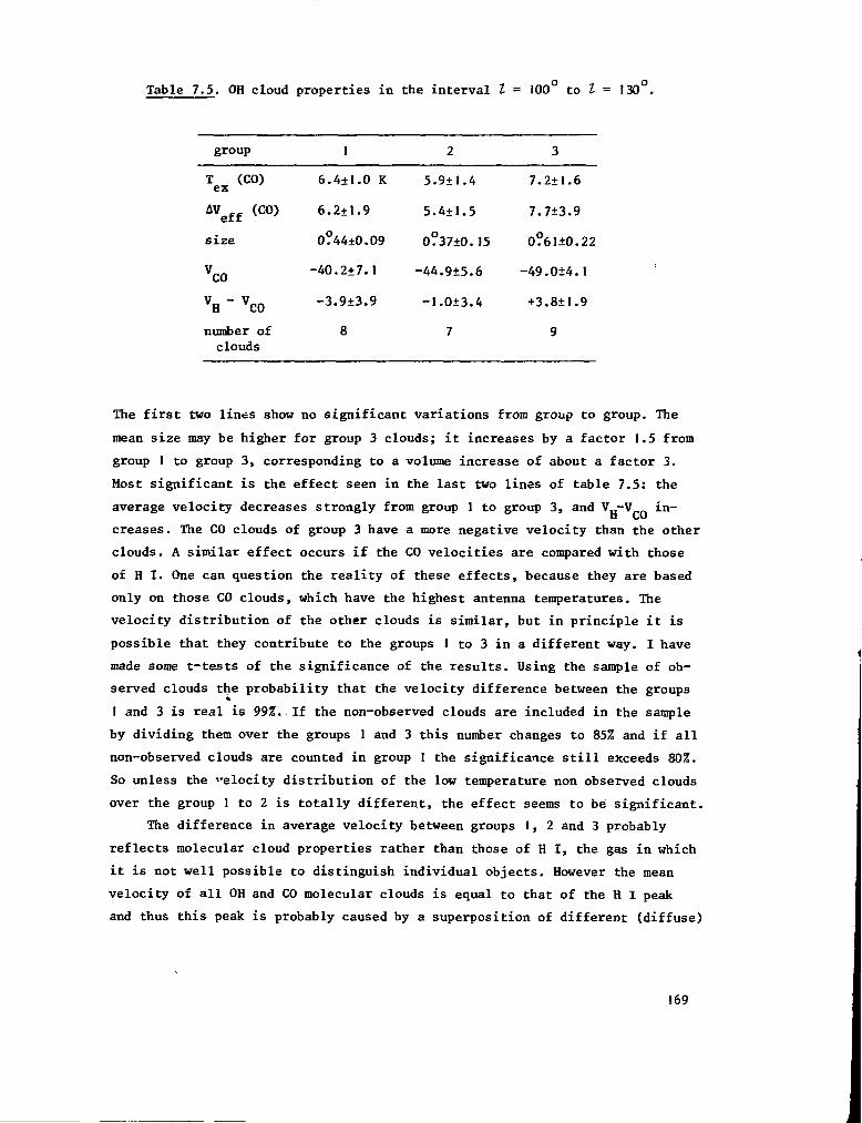
Table 7.5. OH cloud properties in the interval t = 100 to 1 = 130 .

group

T (CO)ex

AVeff (CO)

size

vcoVH " VC0

number ofclouds

6.4±1.0 K

6.2±1.9

0?44±0.09

-40.2±7.1

-3.9±3.9

8

5.

5.

0?

-44

-1

9±1.4

4±1.5

37±0.15

.9+5.6

•0±3.4

7

7.2±1.6

7.7+3.9

0?61+0.22

-49.0i4.l

+3.8±1.9

9

The first two lines show no significant variations from group to group. The

mean size may be higher for group 3 clouds; it increases by a factor 1.5 from

group 1 to group 3, corresponding to a volume increase of about a factor 3.

Most significant is the effect seen in the last two lines of table 7.5: the

average velocity decreases strongly from group 1 to group 3, and V -V_. in-H CO

creases. The CO clouds of group 3 have a more negative velocity than the other

clouds. A similar effect occurs if the CO velocities are compared with those

of H I. One can question the reality of these effects, because they are based

only on those CO clouds, which have the highest antenna temperatures. The

velocity distribution of the other clouds is similar, but in principle it is

possible that they contribute to the groups 1 to 3 in a different way. I have

made some t-tests of the significance of the results. Using the sample of ob-

served clouds the probability that the velocity difference between the groups

1 and 3 is real is 99%. If the non-observed clouds are included in the sample

by dividing them over the groups 1 and 3 this number changes to 85% and if all

non-observed clouds are counted in group 1 the significance still exceeds 80%.

So unless the velocity distribution of the low temperature non observed clouds

over the group 1 to 2 is totally different, the effect seems to be significant.

The difference in average velocity between groups 1, 2 and 3 probably

reflects molecular cloud properties rather than those of H I, the gas in which

it is not well possible to distinguish individual objects. However the mean

velocity of all OH and CO molecular clouds is equal to that of the H I peak

and thus this peak is probably caused by a superposition of different (diffuse)

169

clouds and not by velocity crowding. At the positions of four clouds from

group 3 the 21 cm line profiles show an indication of H I self absorption.

Since at most positions my OH observations are only at the CO peak, a selec-

tion effect could have been introduced, because in some clouds the OH and CO

peak do not agree (e.g. the clouds near the Orion and Rosette Nebulae). How-

ever, this situation appears exceptional and to occur only when the clouds

are associated with strong and large H II regions; such regions are even more

exceptional in the Perseus arm as I will show later.

The most important parameters in which the clouds of groups 1 and 3 are

different are the mass and the mean density. With the present data it is only

possible to make some very crude quantitative estimates of those parameters.

Because group 1 clouds are a factor 1.5 smaller, their volume is on the

average a factor 3 less than those of group 3. The OH column densities in

group 1 and 3 differ by at least a factor 2.5 and thus the masses of the

group I clouds are around 6 times smaller and their mean densities are about

0.5 times those of group 3. This does not exclude the presence of high density

fragments in clouds of each of the groups. Note that these differences will

be much larger if kinematical distances are adopted. I draw cautiously the

conclusion that the kinematic properties of the Perseus arm clouds are corre-

lated with some of their physical properties. Clearly these results have to

be confirmed by OH observations of the rest of the clouds and by 13C0 obser-

vations.

In many cases spiral arms show rolling motions (Harten, 1971; Yuan and

Wallace, 1973). This is concluded from a velocity gradient of the peak H I

velocity in latitude direction over the whole extent of the arms. The mean

velocity of molecular clouds as a function of latitude appears to show a

similar velocity gradient. The mean value obtained from the CO data between

I = 108° and I = 113° is -3.3 ± 1.0 km s"1 deg"1. From 21 cm line observa-

tions, Harten obtained the values -1.8, -2.6 and -3.0 km s"1 deg"1 at

I = 105 , 110 and 115 respectively, in good agreement with my conclusion.

It also follows that the relation between V - V„ and cloud properties isUH n

not affected by the rolling motions. A similar velocity gradient seems also

present in other longitude intervals. An uncertain estimate in the interval

from I = 120° to 128° is -4.3 ± 1.0 km s"1 deg"1, where the H I gradient is

-2 ± 1 km s"1 deg"1. Remarkable is that in this longitude range also the

supergiant stars in the data by Humphreys (1976) show such a latitude gra-

dient (-2.3 km s"1 deg"1), although such a gradient does not exist around

I = 110 . I consider the reality of the gradient for the stars to be doubtful

until more data are available.

To study the relation between the molecular clouds and H II regions I

used radio continuum surveys. Recently Kallas and Reich (1980) made a 21 cm

continuum surve of the galactic plane between Z = 90 and 1 = !62 with a

sensitivity limit of 0.3 Jy for point sources and a resolution of 9*. Of all

the molecular clouds in the Perseus arm between I = 104 and Z- = 130 only 11

(y 25%) are associated with a radio source, 8 of which coincide with an opti-

cal H II region. Of the remaining 3 sources one is very weak and possibly not

real. Five of the clouds are too near to Cas A to obtain information on the

radio continuum associated with the clouds. Because some of the 3 new sources

near the clouds may be non thermal background sources, it is clear that there

are only few unknown larger H II regions associated with the clouds. Of course,

many of the clouds may be associated with compact H II regions which escaped

detections in these radio continuum survey because of their small size. Price

(1981) published maps of extended IR sources along this part of the galactic

plane at 11 and 20 um. He detected several sources but the published data are

not sufficiently detailed to make a useful comparison.

7.5.2. The structure of the Perseus arm.

Figure 7.9 displays the positions of a large number of different objects

located in the Perseus arm between I = 100 and I = 140 . Shown are H II

regions (Georgelin, 1975; Crampton et al., 1978; Humphreys, 1976), molecular

clouds (Cong, private communication), young clusters (Georgelin, 1975;

Humphreys, 1976), individual members of OB associations (Humphreys, 1978) and

supernova remnants (Milne, 1979; Kallas and Reich, 1980; Hughes et al., 1980).

The halfwidth of the distribution in latitude is equal for clouds and H II

regions: about 120 pc. Contrary to the local arm, the relation between 0B

associations and molecular complexes remains unclear in the Perseus arm, be-

cause many clouds and H II regions are seen in projection against each asso-

ciation. Exceptions are Cas OB 6, which is related to the W4 complex and

Per OB 1 which apparently is not related to any other object. Cep 0B 5 and

Cas 0B 8 show no clouds, projected within their boundaries, although the ex-

perience with local associations points out that even this is sometimes not a

good criterium. Blaauw (1962) proposed that two H I complexes at about b =

-12 may be related with Per OB 1. The region of these clouds is outside the

171

6.0

2.0

-20

-6.0

6.0

2.0

-2.0

-6.0 -

I l l

3C58

S183,

W5 Wt W3

\ i

M 1 I I ) I I M \2 00 pc

I 11 1 F \

I I I

^ * • * : • *

i i i i i

IVO 136 132 128 124 120 116 112 108 1 DU 100

Figure 7.9. The distribution of Perseus arm objects. Shown are OB stars

(small +)3 young clusters (large +), E II regions (*), molecular

clouds (L) and supernova remnants (0). In the upper part of this

figure the extent of the associations is indicated, together with

the position of some individual objects.

area, surveyed for OH. If there is a relation, the distance between cloud and

association is much larger (% 350 pc) than typical for those complexes in the

lccal arm, but, of course, the clouds are exceptionally far away from the

galactic plane. For the other associations the number of clouds, which may be

related to them, can be decreased somewhat if one compares the radial veloci-

ties of cloud and association (Humphreys, 1976). However one has to keep in

mind that the difference between the two velocities is sometimes large (e.g.

10 km s"1 for Per OB 2). Therefore I shall give for the other associations

the number of possibly related clouds for velocity differences of 10 and

2 km s"1. Cep OB 1: 6 and 3; Cas OB 2: 7 and 2; Cas OB 5: 5 and 2; Cas OB 4:

2 and 1; Cas OB 7: 4 and 4; Cas OB 1: 1 and 0. On this basis I can give only

some "best candidates". These are for Cep OB 1: cloud 3 and 5 (from table 7.3);

172

for Cas OB 2: cloud 7; for Cas OB 5: cloud 17; for Cas OB 4: cloud 19; for

Cas OB 7: cloud 22 and for Cas OB I: a cloud which was not observed in OH at

(125.0, -0.25). It is remarkable that of these 7 clouds, 4 are related with

an H II region. This further selection was based on size and CO temperature,

but these are not necessarily the best criteria. Many of the local associa-

tions are much smaller than the several hundreds of parsecs which the Perseus

arm associations measure (see table 8.3). Because the distances of most asso-

ciations are almost equal, a more careful study will be necessary to define

the extents of the associations. In figure 7.9 I have included the supernova

remnants (SNR) because they may function as triggers of star formation. There

are 10 SNR's known in the direction of the fragment of the Perseus arm dis-

cussed here. They are equally distributed in longitude but four of them (all

around Z- = 130 ) are outside the boundaries of the associations. However, the

SNR ages are probably to small to show any noticeable effect on the clouds.

The Perseus arm has two major concentrations of young objects around

1 = 110 and near Z = 134 . The surface number density of H II regions and

molecular clouds is a factor 2.5 to 3 larger around I = 1.10 than on the

average in the Perseus arm. Also the W3/W4/W5 area is outstanding against

lower and higher longitudes. The separation between the two concentrations is

about 1500 pc at 3.5 kpc distance. Similar concentrations are observed in

other galaxies at typically the same distance. The properties of H II regions

along the arm can be analysed in some detail using the survey of Kallas and

Reich (1980). I divide the area into two parts: 103° < I < 114° and 114° < I

< 130° that contain almost equal numbers of (visible) H II regions: 16.

In the first part 15 H II regions were detected by Kallas and

Reich compared to 10 in the second part. This indicates that, on average,

the first part has stronger radio emission. (It did not seem meaningful to

obtain a direct average flux density in the two areas because of the high

values of some single regions.) A second result is that in the first part of

the arm 6 H II regions are larger than 30 arcmin. whereas there are only 2

in the second part. In addition the first part also contains point sources.

Optically there are also differences among the M II regions. From the cata-

logue by Sharpless (1959) one can find that the M II regions between I = 108°

and 114 preferentially are listed in the categories "brightest" and "fila-

mentary" whereas in the other part more regions are listed as "faintest" and

"amorphous". One can obtain an indication of the relative ages of the associ-

ations in the Pereus arm by comparing the distributions of the stars over

173

spectral types, as published by Humphreys. As far as the division in O and B

stars is concerned, this does not result into appreciable differences, except

for Cas OB 6, which contains twice as much 0 stars as B stars. A probably more

significant result is that the three stars of earliest spectral type are on

the average later (09 to B2) for associations in between the concentrations

(Cas OB 4, Cas OB 7, Cas OB 1, Cas OB 8 and Cep OB 5) than for those in or

near concentrations (05 to 08). This indicates that the concentrations may be

the younger parts of the arm. In addition to the contrast between a "concen-

tration" (108 < 'I < 114°) and a more conspicuous part of an arm (114 < I

< 130 ), there is also a difference in H II regions between the two concentra-

tions: the one around I = 110° and the one near I = 134°. H II regions near

I = 110° are much smaller. This can be an age effect: the H II regions in the

area around I = 110 might be younger on the average than those in the W3/W4/

W5 area around I = 134 . In both concentrations is star formation going on

as shown by the presence of OH and H.O maser sources. These are not known at

other longitudes. The two maxima at I = 110 and I = 135 are also visible

in the H I distribution, probably because the molecular clouds are surrounded

by large H I clouds. The clouds of the concentration of molecular clouds near

Z- = 110 , are kinematically not different from those in the rest of the

Perseus arm. I do not know whether more such concentrations as the two dis-

cussed here exist farther down or up the Perseus arm because the other parts

have not been studied as well. Around 1 = 155 there is a concentration of

radio sources in the survey of Kallas and Reich where Cong (private communi-

cation) detected some molecular clouds. Probably this concentration is not as

pronounced as the two discussed here. At lower longitudes only a few data

concerning the Perseus arm are available. A group of H II regions at 8 or 9

kpc distance is present at I = 70° in the area of W 58 (Israel, 1976), which

is another area of activity like the W3 area.

The only mechanism to form concentrations of this scale length which has

been suggested sofar, is Parker's instability (Parker, 1966), in which the semi-

equilibrium state of magnetic and gravitational field becomes unstable after

which interstellar matter slides down along the field lines toward the positi-

on of the concentration. A recent discussion of this instability was given by

Mouschovias (1981). The scale length of this effect is expected to be of the

order of 1 kpc. Observationally this mechanism is not yet very well supported.

Observations of the magnetic field direction, near the Perseus arm (optical:

Matthewson and Ford, .1970 and radio: Brouw and Spoelstra, 1976) do not show

174

deviations from the general pattern in the vicinity of the concentrations, but

it is quite possible that both types of observations do not reach sufficiently

far out. The mean relative distance of molecular clouds in the Perseus arm is

around 200 pc if I assume a depth along the line of sight of 1 kpc. Since this

is even less than Blitz's (1978) value for the local spiral arm (500 pc) it

is unlikely that the individual clouds arise from Parkers mechanism (this is

also a conclusion by Mouschovias, 1981).

Several models have been suggested that explain the structure of this

part of the Perseus arm (Rickard, 1968; Roberts, 1972; Verschuur, 1973; Rohlfs,

1974; Burton and Bania, 1974). However, non of these authors incorporated the

properties of the molecular clouds, because these were not yet known. To form

a basis for a discussion of these models I now list relevant facts that have

to be explained and I review which of the models can explain the facts. I

first list results from the present observations. Second I recapitulate im-

portant properties of Perseus arm objects obtained previously by others and

third, for completeness, some additional properties of less importance,

la. The mean velocity of H I is the same as that of all molecular clouds,

lb. The larger and more massive clouds ("group 3") have a more negative radial

velocity than clouds of lower mass ("group 1").

lc. H II regions do not occur preferentially near clouds of group 1 than near

clouds of group 3. Also there are no differences in properties between

those H II regions associated with group 1 and those with group 3.

Id. The absence of molecular clouds between -20 and -40 km indicates that

molecular clouds of the size that has been detected in CO and OH are at

least a factor 5 less abundant in the interarm region than in the arm

(this is a conclusion of Cohen et al. 1980).

le. A weak anti-correlation exists between the positions of molecular clouds

and the projected early type star density in a field around Z = 110

(Wramdemark, 1981).

The interpretation of point Id. is still uncertain. Liszt and Burton (1981)

showed that the kinematics can have as important consequences for the observed

velocity distribution as the density contrast.

Important results from other authors are:

2a. The radial velocity of stars at the near side of the arm are closer or

much closer (I = 120° - 130°) to that of the clouds than the velocity of

the far side stars (Humphreys, 1976). There is an indication that the

earliest type stars have a more negative radial velocity (Martin, 1972).

175

2b. Hie distribution of extinction with distance varies in character from

one region to the other. Characteristics for three different regions are:

a. it is constant, independent of distance, b. it shows a steady increase

with distance, and c. it shows a discontinuity of 0.5 to 1.5 magnitudes at

around 2 to 3 kpc distance (Wramdemark, 1976, 1981; Martin, 1972; Neckel

and Klare, 1980).

2c. The space density of early type stars and H II regions has a maximum at a

distance of 3 kpc with a very sharp decline (Georgelin, 1975; Crampton et

al., 1978; Wramdemark, 1976, 1981).

The third group of arm properties are the following:

3a. The mean velocity of all Perseus arm H II regions is on the average A.3

km s"1 more negative than that of all molecular clouds in the same longi-

tude interval (I = 100 to 120 ). This agrees with the observations by

Israel (1976); it supports the "blister model" for H II regions, but it

also indicates that kinematic distances for B II regions are less reliable.

3b. The apparent internal velocity dispersion of molecular clouds, H II regi-

ons, associations and clusters is the same (about 7 km s"1).

3c. Some stars show optical absorption lines with a more negative velocity

than that of the stars (Munch, 1957). The mean value is -51.4 ± 10.5

km s"1. Perhaps these lines occur in two velocity groups.

3d. The rotation curve probably is flat outside the solar circle (Georgelin,

1975; Blitz, 1979). If this is true the average kinematical distance of

Perseus arm objects would become several kiloparsecs larger than the

average distance of optical spiral arm tracers.

3e. Perhaps a secondary maximum of early type stars and H II regions exists

at 5 to 6 kpc distance. However, the numbers of objects are very scall.

The distances of most of the objects placed in this larger distance arm

by Felli and Harten (198I) are kinematical and hence very uncertain.

3f. Local OB associations sometimes are associated with an expanding gas shell

(see chapter 4) with expanding velocities around 10 km s"1.

I will now discuss the consequences of these results for the structure of the

Perseus arm. Without considering kinematical distances the points la, le, 2b

and 2c indicate that there exists a region where H I, molecular clouds and

early type stars coexist. This region is at a distance of about 2.5 to 3.5

kpc and probably has a depth of about 1 kpc. The mean distance between mole-

cular clouds of the type detected in CO and studied in this chapter is 200 pc

and perhaps a factor two smaller in some specific areas as was discussed in

176

the preceding subsection. This does not rule out the presence of many much

smaller features. In fact these features (down to sizes of 1 pc) are detected

through interferometric H I absorption studies as made by Greisen (1973) and

by Read (1980). The results of the measurements of extinct'on as a function

of distance indicate that outside the clouds, the space inside an arm is not

very different from the space in the interarm area. If I take 0.4 as a typical

cloud size, the fraction of the volume of space inside the arms and filled

with molecular clouds is 1.5 x I0~3. This is a factor two larger than the mean

value for local clouds obtained with the data of chapter 6, 8 * 10~\ In the

Perseus arm this number is a lower limit because of the possible presence of

smaller clouds, but it also may be an upper limit if the line of sight depth

of the arm is larger than the adopted 1000 pc. For the area at 5 to 6 kpc

from the galactic center Liszt and Burton (1981) obtained a volume filling

factor of 7 x 10~3.

The discussion of the velocity structure of the arm can be split into two

parts: first a discussion of the velocity gradient or' the arm in latitude

direction and secondly the internal velocity structure. The gradient of the

velocity in latitude is explained in two ways. One possibility is the effect

of perspective due to warping of the galaxy (Yuan and Hallace, 1974). A second

possibility is mentioned by Harten (1971): the position of the center of the

Shockwave and of the distribution in latitude of the molecular gas is not

the same, so the clouds feel an unequally strong shock. The validity of this

model can be tested be deriving the distribution in latitude of late type

stars in the direction of the Perseus arm, but it will be very difficult to

obtain significant results at such a large distance. The distribution of the

velocities of the molecular clouds and of H I in the direction of the Perseus

arm in my opinion indicates that H I and molecular clouds coexist at the same

distance along the line of sight. The differences in radial velocity indicate

that along the line of sight more than one H I cloud exists, one of which

perhaps is partly molecular and detected during the survey. Any variation of

the cloud velocity with time is also experienced by the H I: in a given volume

of space the clouds and H I do not move with respect to each other.

Different models have been made of the structure of the Perseus arm. I

will discuss a few. (i). Rickard (1968) explained the distribution of stellar

velocities, those of H I and of the interstellar absorption lines (point 3c)

by a super-super nova explosion that has occurred within the arm. I think this

solution is too drastic, (ii). Since this super-super nova explosion appears

177

quite an ad-hoc explanation and other explanations work quite well, I reject

Rickard's hypothesis- Verschuur (1973) postulates, from measurements at higher

latitudes, the existence of another spiral arm, the a-arm, behind the Perseus

arm. The H I gas at b = 0 , usually ascribed to the Perseus arm would belong

to the a-arm, whereas the H I gas around -40 km s"1, detected at b = +5 to

10 , should form the backside of the Perseus arm. The clouds at high negative

velocities, detected by Munch (1957) would be at the frontside of the Perseus

arm, expelled by one big H II region which is formed by all associations and

young clusters in this area. Verschuur's model is not in agreement with the

present observations because of the velocity distribution of molecular clouds

and H I gas and because some clouds are associated with H II regions. (Hi).

Burton and Bania (1974) and Rohlfs (1974) analysed the H I gas and the stars

(Burton and Bania) in connection with deviations from the Schmidt rotation

curve. The perturbations from this curve which Rohlfs obtains indicate the

presence of a shock at 2 kpc distance and of an H I maximum at 4 kpc distance

from the sun, which is behind the stellar arm. Burton and Bania found that a

better correlation between stars and gas results if the rotation curve is

steeper than that of Schmidt. This is in contrast with recent results (Blitz,

1979) which indicate that the curve is flatter outside the solar circle.

The present observations in my opinion agree best with the model by

Roberts (1972), who included the effects of a galactic spiral shock upon the

Schmidt rotation curve. In this model the clouds are formed at a post shock

velocity of -50 to -55 km s"1. When tnese clouds subsequently move through

the spiral arm their velocities become less negative. Ultimately the clouds

form stars between radial velocities of -50 and -35 km s"1. In spectra of

these stars Münch (I957) detected more negative velocity absorption lines

which are caused by clouds in front of the stars. (These lines can be explained

also by an expanding shell around the association; see point 3f). Some addi-

tional calculations have been made by Bash (private communication). Using the

results from Bash and Peters (1976) in this part of the galaxy he found that

there should be a radial velocity difference of 10 to 15 km s"1 between newly

formed clouds and the stars. In this picture the less negative velocity clouds

are older. However the Bash calculations do not explain the presence of clouds

with a different radial velocity in concentrations like the one at I = 110

because those clouds should have originated at different longitudes. According

to the model by Roberts the clouds of group 3, which are more massive and have

the most negative velocity would have been formed most recently and thus they

178

are quite young. The clouds of group 1 are partially older and less massive

because they have formed stars and a smaller (because velocity changes are

more rapid) part can be younger because they are in front of the galactic

shock; ultimately these will form the group 3 clouds. The presence of H II

regions near group 3 indicates that the onset of star formation has to be

fairly rapid after the formation of these clouds because the velocity changes

are of the order of 1 km s"1 per I06 yr.

Instead of developing these somewhat qualitative considerations, further

I propose to wait for more detailed observations: the distribution of cloud

mass with radial velocity is one of the parameters that one would like to

know better. Another thing is the number and the properties of interarm clouds

which should be observable at low radial velocities. One has to study age and

extent of the associations better. The properties of stars with a high and

with a low radial velocity have to be analysed as well as the direction of the

magnetic field at about 3 kpc distance. It is possible to make a comparable

study of a part of the Carina arm between Z = 300 and I = 20 . Because this

arm is somewhat closer and other spiral arms are located behind it, the inter-

pretation will be more complicated than in the case of the Perseus arm.

7.6. Conclusions.

I have made a survey of the Perseus arm molecular clouds. Five large

clouds were detected in Dwingeloo and mapped in Effelsberg. They have masses

of the order of a few times 101* M_. The clouds show little internal velocity

structure. The cloud near W3 shows very strong thermal emission at one posi-

tion. The spectrum of the 1720 MHz OH maser near NGC 7538 shows much struc-

ture. In addition there are many smaller clouds found by Cong in CO. I ob-

served a part of the CO clouds in this arm in OH. A new, -weak type I OH maser

was detected near S 152. There appears to be a correlation between the detec-

tions of OH clouds and radial velocity: clouds with a larger OH column density

(and probably a larger mass) have a more negative radial velocity. A tentative

explanation is presented in terms of the model of the arm by Roberts. The mean

number density of this kind of clouds is probably larger in the Perseys arm

than in the local arm but less than in the "molecular ring" at 5 kpc from the

Galactic Center. The arm-contains concentrations of H II regions and molecu-

lar clouds, which differ in age and cloud density, but not in kinematics from

179

the rest of the arm. The ensemble of clouds show a velocity gradient in lati-

tude direction, similar to the H I.

References.

Bash, F.N., Peters, W.L., 1976, Astrophys. J. 205, 786.

Blaauw, A., 1962, in Interstellar Matter in Galaxies, ed. L. Woltjer, p. 63.

Blair, G.N., Peters, W.L., Vanden Bout, P.A., 1975, Astrophys. J. 200, L 161.

Blitz, L., 1978, thesis, Columbia university.

Blitz, L., 1978, Asti -?phys. J. 231, L 115.

Braunsfurth, E., Reich, W., Rohlfs, K., 1979. Mitt. A.G. 45, 91.

Brouw, W., Spoelstra, T.A.Th., 1976, Astron. Astrophys. Supp. 26_, 129.

Burton, W.B., Bania, T.M., 1974, Astron. Astrophys. ̂ 3, *25>

Cohen, R.S., Cong, H., Dame, T.M., Thaddeus, P., 1980, Astrophys. J. 239, L 53.

Crampton, D., Georgelin, Y.M., Georgelin, J.P., 1978, Astron. Astrophys. 66_, 1.

Felli, M., Harten, R.H., 1981, Astron. Astrophys. 100, 42.

Forster, J.R., Goss, W.M., Wilson, T.L., Downes, D., Dickel, H.R., 1980,

Astron. Astrophys. J34_, L 1.

Gahm, G.F., Lindroos, K.P., Sherwood, W.A., Winnberg, A., 1980, Astron. Astro-

phys. J$3, 263.

Georgelin, Y.M., 1975, thesis, Université" de Provence.

Georgelin, Y.M., Georgelin, Y.P., 1976, Astron. Astrophys. 49_, 57.

Goudis, C , 1979, Astrophys. Space Sci. 6\_, 417.

Greisen, E.W., 1973, Astrophys. J. 184, 379.

Hasegawa, T., Sato, F., Fukui, Y., 1980, Interstellar Molecules, ed. B.H.

Andrew, p. 159.

Hardebeck, E.G., 1971, Astrophys. J. 2Z0, 281.

Harten, R.H., 1971, thesis, University of Maryland.

Höglund, B., Gordon, M.R., 1973, Astrophys. J. 182, 45.

Höglund, B., Andersson, C , 1974, Astron. Astrophys. ̂ 3» 389.

Hughes, V.A., Harten, R., Van den Bergh, S., 1981, Astrophys. J. 246, L 127.

Humphreys, R.M., 1976, Astrophys. J. 206, 114.

Humphreys, R.M., 1978, Astrophys. J. Supp. ̂ 8, 309.

Israel, F.P., 1976, thesis, Leiden University.

Israel, F.P., 1977, Astron. Astrophys. 6^, 377.

Israel, F.P., 1978, Astron. Astrophys. 70, 769.

180

KaHas, E., Reich, W., 1980, Astron. Astrophys. Suppl. 42^ 227.

Lada, C.J., Elmegreen, 8.G., Cong, H.I., Thaddeus, P., 1980, Astrophys. J.

266, L 39.

Liszt, H.S., Burton, W.B., 1981, Astrophys. J. 243, 778.

Lo, K.Y., Burke, B.F., Haschick, A.D., 1975, Astrophys. J. 202, 8.

Martin, N., 1972, Astron. Astrophys. \7_, 253.

Matthewson, D.S.., Ford, V.L., 1970, Mem. Roy. Astron. Soc. _74> 139.

Milne, D.K., 1979, Aust. J. Phys. ̂ 2 , 83.

Minn, Y.K., Greenberg, J.M., 1975, Astrophys. J. J96_, 161.

Mouschovias, T.Ch., 1981, in Fundamental problems on the theory of stellar

evolution, ed. D. Sugimoto, D.Q. Lamb, D.N. Schramm, p. 27.

Munch, G., 1957, Astrophys. J. J73, 259.

Neckel, Th., Klare, G., 1980, Astron. Astrophys. 42^ 251.

Parker, E., 1966, Astrophys. J. 145, 811.

Price, S.D., 1981, Astron. J. 86_, 193.

Read, P.L., 1980, Mon. Not. R.A.S. J92, 11.

Rickard, L.J., 1968, Astrophys. J. _I52, 1019..

Rickard, L.J., 1979, in The large scale characteristics of the Galaxy, ed.

W.B. Burton, p. 413.

Rohlfs, K., 1974, Astron. Astrophys. _35_, 177.

Rohlfs, K., Braunsfurth, E., Hills, D.L., 1977, Astron. Astrophys. Supp. 30,

369.

Roberts, W.W., 1972, Astrophys. J. IT3, 259.

Sharpless, S., 1959, Astrophys. J. Supp. 4, 257.

Stark, A.A., 1980, thesis, Princeton University.

Turner, B.E., 1979, Astron. Astrophys. Supp. 3_7, ••

Verschuur, G.L., 1973, Astron. Astrophys. 24_, 193.

Heaver, H., 1974, Galactic radio astronomy, ed. F.J. Kerr, S.C. Simonson III,

p. 573.

Wendker, H.J., Altenhoff, W.J., 1977, Astron. Astrophys. 54_, 301.

Westerhout, G., 1972. Maryland-Greenbank 21 cm survey, 2nd ed. University of

Maryland.

Wratndemark, S., 1976, Astron. Astrophys. Supp. 26_, 31.

Wramdemark, S., 1981, Astron. Astrophys. Supp. 43, 103.

Wynn-Williams, C.G., Werner, M.W., Wilson, W.J., 1974, Astrophys. J. 187, 41.

Yuan, C , Wallace, L., in Galactic Radio Astronomy, ed. F.J. Kerr, S.C.

Simonson, III, p. 591.

181

CHAPTER VIII

IMPLICATIONS OF THE OH STUDIES FOR THE STRUCTURE OF MOLECULAR CLOUDS

8.1. Introduction.

In this chapter I try to synthesize the results of the observations de-

scribed in the preceding chapters. First in 8.2 I discuss the general results

in connection with OH excitation temperatures and optical depths. Then I dis-

cuss the structure of large molecular clouds: in 8.3 the morphology, in 8.4

the mean densities, the density distribution and the interval velocities. In

8.5 I compare the OH results with H I and in 8.6 with CO observations. In 8.7

I discuss the occurrence of velocity gradients in local clouds and in 8.8 the

compatibility of all my results with different existing models of the formation

of such clouds. I conclude in 8.9 with some suggestions for further research

of OH clouds.

8.2. The excitation conditions of the OH molecules.

In this section I summarize the general results of the OH observations

relating to the derived parameters T, and T .. In table 8.1 in columns 2

and 3, I have collected the average data in the different cloud centers where

in most cases all four OH lines have been observed. The most important result

in table 8.1 is that the excitation temperature increases when the linear

beamsize decreases and that T _ is very low; implicit in the method of ana-

lysis is that T „ becomes smaller if at the same optical depth, T _ isex,J A,j

smaller. To facilitate the discussion I have also listed in columns 7 and 8

the results of the highest resolution OH observations that exist in the differ-

ent areas. I have included the data by Mattila et al. (1979) on L 134 because

this is a single cloud that may be typical for fragments within the complexes.

The highest antenna temperatures vary between 0.8 K and 1.0 K for regions

where the resolution varies between 0.1 .pc and 0.8 pc. Unfortunately the opti-

cal depths could not be determined accurately except for L 134. Averages over

183

Table 8.1. General results on the excitation of OH.

complex

Mon OB 2

L 1605

L 1626

Ophiuchus

Taurus A

L 134

T3

1.5

0.6

1.2

.0.5-2

1-3

1.2

Tex,3

3.5

3.7

3.6

3.9-3.

3.9-3.

5.0

7

7

DT

-

-

-

<0.5

0

-

TA, 3

<0.1

0.1

0.1-0.

0.1-0.

0.2-0.

-

2

3

3

Res.

13

7

7

1.

1.

pc

,5

(0

\

0

0

0

0

3 max

-

-

.70 .

.9

.85

.97

0

0

0

0

Res

.79 pc

.39

.11

.23

O)(2)

(1)

(3)

(1) Lang and Willson (1979)

(2) Myers et al. (3 978)

(3) Mattila et al. (1979)

a large number of positions suggest a value of x, rather similar to the value

obtained in chapter 3 for the NGC 2264 area and in chapter 5 for the Taurus

area. Typical antenna temperatures near, but outside the maxima are 0.3 to

0.4 K. These results indicate that the filling factor for the Dwingeloo obser-

vations is significant say F = 0.5 and for the high-resolution observations

F = 1.0. A determination of T , for the high resolution observations has onlyex, j

been made for L 134 by Mattila et al. They deduce a value of T ., = 5 ± 0.5 K,comparable with values of T . in more diffuse clouds in front of continuum

ex, J

sources (Dickey et al. 1981), where T , is 5 to 6 K, but much higher than

those in table 8.1. It is possible that in the center of the cloud a combina-

tion of a higher density and a lower kinetic temperature gives a somewhat

lower excitation temperature, but the excitation temperatures derived from the

Dwingeloo observations are too low to be explained in this way. This can be re-

solved by assuming that F is smaller than 1.0., which is quite reasonable as

said before. If I take F = 0.5, T will be typically 4 to 4.5 K and forex, J

F = 0.25 it is about 5 K in the Taurus and Ophiuchus clouds. (_ For this reason

the concept of "the excitation temperature" loses some significance when de-

rived from Dwingeloo observations, because it is a mean of excitation tempera-

tures in the fragments and in the less dense common envelope of these frag-

ments.3 If F < 1 the mass of the cloud is smaller than derived for F = 1.

184

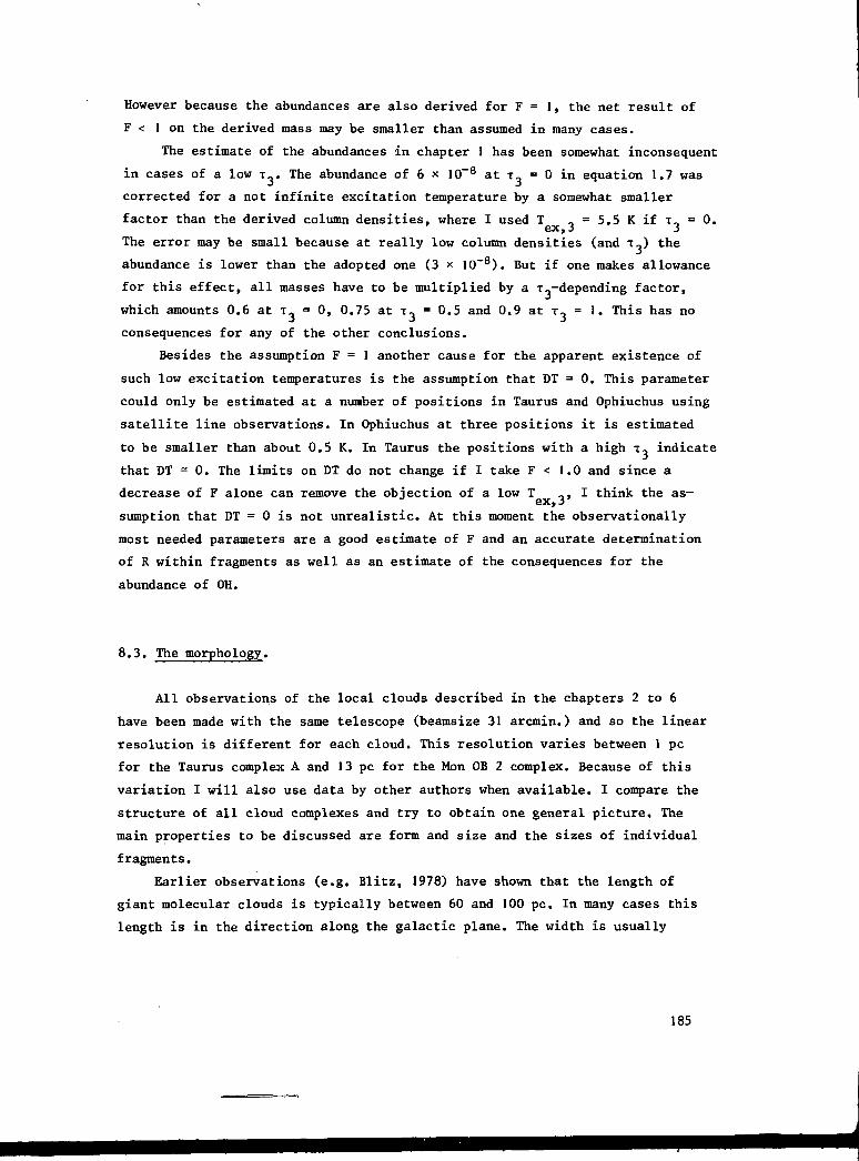
However because the abundances are also derived for F = 1, the net result of

F < 1 on the derived mass may be smaller than assumed in many cases.

The estimate of the abundances in chapter 1 has been somewhat inconsequent

in cases of a low x„. The abundance of 6 x 10~8 at x, = 0 in equation 1.7 was

corrected for a not infinite excitation temperature by a somewhat smaller

factor than the derived column densities, where I used T _ = 5.5 K if T = 0.

The error may be small because at really low column densities (and x_) the

abundance is lower than the adopted one (3 x 10~8). But if one makes allowance

for this effect, all masses have to be multiplied by a x--depending factor,

which amounts 0.6 at x_ = 0, 0.75 at T , = 0.5 and 0.9 at x., = 1. This has no

consequences for any of the other conclusions.

Besides the assumption F = 1 another cause for the apparent existence of

such low excitation temperatures is the assumption that DT = 0. This parameter

could only be estimated at a number of positions in Taurus and Ophiuchus using

satellite line observations. In Ophiuchus at three positions it is estimated

to be smaller than about 0.5 K. In Taurus the positions with a high x~ indicate

that DT - 0. The limits on DT do not change if I take F < 1.0 and since a

decrease of F alone can remove the objection of a low T ,, I think the as-ex, j

sumption that DT = 0 is not unrealistic. At this moment the observationally

most needed parameters are a good estimate of F and an accurate determination

of R within fragments as well as an estimate of the consequences for the

abundance of OH.

8.3. The morphology.

All observations of the local clouds described in the chapters 2 to 6

have been made with the same telescope (beamsize 31 arcmin.) and so the linear

resolution is different for each cloud. This resolution varies between 1 pc

for the Taurus complex A and 13 pc for the Mon OB 2 complex. Because of this

variation I will also use data by other authors when available. I compare the

structure of all cloud complexes and try to obtain one general picture. The

main properties to be discussed are form and size and the sizes of individual

fragments.

Earlier observations (e.g. Blitz, 1978) have shown that the length of

giant molecular clouds is typically between 60 and 100 pc. In many cases this

length is in the direction along the galactic plane. The width is usually

185

between 10 and 20 pc and the complexes are thus rather elongated. The complexes

•show structure at different scales. The largest scale related to the complex

is the H I cloud which surrounds the molecular complex; I discuss the H I ob-

servations further in section 8.6. The largest clouds sometimes consist of two

separate complexes as in the case of Mon OB 1 and Ori OB 1. Within each com-

plex the structure at the largest scale is defined by the distances between

those main peak that show up in low resolution observations. The mean values

of the distances between neighbouring peaks for a number of complexes are

shown in table 8.2 and are typically 10 ± 2 pc, although in the Ophiuchus com-

plex the average is a factor two smaller. The borders of the emission associa-

ted with these peaks are often difficult to define because these areas are

embedded in a cloud of extended emission, but they have sizes between 3 and

10 pc. This 10 pc structure also has been found by Blitz, but because his12C0 observations probably reflect predominantly temperature variations in-

stead of density variations, the interpretation of the CO observations is less

certain. Because the 10 pc structure is also found in OH and in observations

with varying linear resolution (0.6 to 4 pc). I think it is clear that giant

molecular clouds are not uniform, but consist of a few large clumps.

Even smaller scales of cloud structure can be recognized. The 10 pc frag-

ments in Taurus (chapter 5) show clumps of the order of 2 to 3 pc in size.

Blitz found this also in those parts of the Mon ON 1 and 2 complexes where he •

made higher resolution observations. Detailed observations of total complexes

take much observing time and these observations are thus possible for only a

few fragments. It is therefore difficult to obtain an overall picture of such

complexes (except for the Taurus complex). But incidental observations in

other areas (e.g. Minn and Greenberg, 1979) in Mon 0B 1 or in other complexes

(e.g. Few and Booth, 1979) in Ori OB 1, show that it is probable that their

structure is similar to that in Taurus. Small-scale structure is studied quite

well in some selected areas of cloud complexes. A few examples are Cloud 2

(Sume et al., 1975), the area near NGC 2264 (Crutcher et a., 1978), the p Oph

cloud (Myers et al., 1978). These areas show structures of about 1 pc in size.

Interesting is also L 134 (Mattila et al. 1979), which is a single cloud of

about 1 pc. The size spectrum of structure within a molecular cloud has been

measured down to 0.1 - 0.2 pc (high density parts in Ophiuchus, observed in

molecules such as SO and HCN, the carbon chain molecules in Taurus and possibly

H„CO absorption in front of H II regions (Forster et al., 1981). This size of

clouds is mostly studied in the vicinity of H II regions or detected by

186

accident like those in the Taurus clouds. Not much knowledge exists about the

exact spectrum of the size of the fragments in large molecular clouds, and

possible differences between the general complex and areas with star formation:

it is not clear whether all clouds are fragmented down to the level of 0.1 pc.

However at the larger scales all complexes appear to be fragmented and I think

that the differences between the Taurus complex and complexes near OB associa-

tions are not large and only found in relatively small areas where massive

stars form. In the other parts the Taurus complex appears to be rather similar.

The fragments in molecular clouds apparently are organized in two ways.

One can distinguish between clouds without special ordening and dustlanes,

strermers or filaments, where the fragments are aligned along structures with

an axial ratio of about 1 : 10. Examples of the last type of organisation are

the dust lanes in Taurus and Ophiuchus. Schneider and Elmegreen (1979) have

made a catalogue of such objects, which they call 'globular filaments'. They

have lengths between 0.5 and 5 . But even at smaller scales these structures

exist: TMC 1 is elongated as well as some small H„C0 features, seen in absorp-

tion in front of DR 21 (Goss, private communication). At even larger scale

Morris et al. (1980) detected CO in this clouds, about 10 long with an un-

known distance. At distances larger than 200 pc it is not well possible to

detect structures, as found in Taurus and Ophiuchus, within a cloud complex

in a large-scale survey because they are narrow (0.5 to 1.5 pc) and because in

CO these structures can be missed through the presence of lower density enve-

lopes.

Probably the nature of the different filaments is not the same: the cores

of the dustlanes in Taurus are much narrower in Taurus than in Ophiuchus (see

plate 3 and 4). The molecular observations indicate that the lanes in Taurus

are embedded in an extended region of lower density, whereas this is probably

not the case in Ophiuchus. This can be due to a different formation mechanism.

Those in Ophiuchus seem to be related to the association (because of their

orientation), whereas in Taurus no association is present and they have to be

formed in another way. Furthermore it seems to be unlikely that the filamen-

tary structures of very different length scales are produced by the same mecha-

nism.

187

8.4. Densities and internal velocities.

Because of the clumpy structure of large molecular clouds it is not rea-

listic to construct models that assume a uniform density. Also one has to use

a mean density depending on the size of structures one is dealing with. From

the observations in the chapters 3 to 5 densities are derived indirectly and

because of the low angular resolution only rough estimates of the mean density

along the line of sight can be obtained. However the mean values are consistent

with results of others. Typical mean densities and masses at different scales

are 50 to 100 cm"3 and 10s M for the whole complex; in the structures with

sizes 'v 10 pc a few times 102 cm"3 and 101* Mfl; for sizes of 2 to 3 pc: about

103 cm"3 and 10 M ; for sizes of 1 pc: 5 x 103 cm"3 and 102 M and for sizes

of 0.2 pc: 105 cm"3 and 1 M . These numbers are however only mean values,

around which considerable spread is present.

In chapter 5 the similarity of the internal structure of large complexes

was shown in figure 5.11, where the log of the surface area T. is plotted

against the antenna temperature T.. All cloud complexes show a straight line

with approximately the same slope. A similar plot for a simple molecular cloud,

e.g. L 134 (Mattila et al., 1979) yields the same result. Since the IXT curve

of a complex is the sum of the curves of its fragments, this makes it possible

that molecular clouds are built up of many L 134 tupe clouds (perhaps with a

range in size). The similarity 2-T. relations in the outer parts of complexes

was already noted by Blitz (1978). I have made a few simple models to help to

interprete these diagrams. I made estimates of the expected distribution of

the OH antenna temperature for spherically symmetric clouds, a constant exci-—01

tation temperature and a density distribution n_„ <* r . For o = 0 and 1 oneUn

finds analytical predictions for the E-T. relation. The case a = 0 predicts a

curve which is too flat in regions with a low antenna temperature in the outer

parts of the cloud, whereas the case a = 1 appears to fit the observed relation

reasonably well. For a = 2 the expected decrease in column density with radius

is too rapid. These results are only preliminary and should be analysed better.

Because the OH abundance probably changes with density, the slope does not

necessarily reflect that of the total hydrogen distribution n(r). Myers et al.

(1978) studied the center of the p Oph cloud and obtained a relation-1 3+0 2

n(r)«r " ~ ' , which however is rather uncertain because it depends stronglyon the relation of extinction with radius, which is only poorly known. For the

—0 9same region near p Oph, Bok (1956) obtained also n = r * , but with the same

188

uncertainties. If clouds are contracting at free fall timescales an o = 2 is

expected. A lower value of a can correspond to retarded free fall (Myers et al.

1978). (Recently Snell (1981) obtained a value 0=2 for some clouds; I have

had no time to analyse why his conclusion differes.)

Another important parameter of the structure of the clouds is the line-

width, which partly reflects internal motions within the complex. There are in-

dications that the linewidths depend on the scale size. Molecular linewidths

averaged over large fractions of cloud complexes (see e.g. chapter 3) are typ-

ically 3 to 4 km s"1. When observed with a smaller linear beamsize generally

the linewidths are smaller. The 2 to 3 pc clouds have a linewidth of 1.5 to

2.0 km s"1 (chapter 5); at 1 pc it is about 0.6 km s"1 (L 134, cloud 2 in

H_CO), and the smallest cloud fragments show 0.2 km s"1 linewidths. However

there are exceptions: the smallest linewidth in Ophiuchus is about 1 km s"1.

These variations indicate that at least a part of the linewidth is caused by

the presence of different "clouds" or "clumps" within the beam. This indication

can be confirmed by making high velocity resolution OH observations in Taurus

with a large telescope (e.g. Arecibo-resolution 0.11 pc) within one or a few

beamwidths of the Dwingeloo telescope. This type of observations might not be

conclusive for OH because existing variations of the linewidth can be distur-

bed by larger scale motions in the lower density interclump medium, which

contributed to the OH emission. This was probably found for different molecules

in Ophiuchus by Myers et al. (1978) and explained by them as cloud contraction.

I have not found in my observations significant variations of the linewidth

in individual complexes.

8.5. The relation between molecular complexes and H I clouds.

Molecular complexes are often accompanied by large H I clouds. These

clouds are visible either in selfabsorption (cloud 2: Wilson and Minn, 1977;

p Oph: Myers et al., 1978; NGC 7538, Read, 1980 and a survey by Liszt et al.,

1981), or in emission (Mon 0B 1, 2: Raimond, 1966; Orion: Gordon, 1980; Taurus:

Sancisi and Wesselius, 1980; Ophiuchus: Strauss et al., 1979; Sancisi and Van

Woerden, 1970). The correspondence in velocity and in extent of self absorbed

H I and molecules (CO, OH) suggest that they are coexisting. The velocity of

the selfabsorption feature often differs somewhat (a few km s"1) from the mean

emission velocity; probably caused by large-scale motion of the gas within the

189

H I complex. Detailed comparisons between selfabsorbed H I and molecules have

been made in some regions. An example is cloud 2 (Wilson and Minn, 1977),

where one of the results was that toward the center of the cloud the H.CO

columndensity increases more rapidly than that of H I, probably because H I is

converted to H„.

Detailed comparisons of H I emission clouds and molecular clouds are dif-

ficult to malse. Promising are the observations of distant molecular complexes

with aperture synthesis telescopes (Read, 1980): the selfabsorption features

of the clouds near NGC 7538 seem to be surrounded by a halo of H I emission.

The molecular complexes in the solar neighbourhood (Orion, Taurus, Perseus)

appear to be situated within, but at the edges of more extended H I complexes.

Observations of the Taurus complex in H I have been made by Sancisi and

Wesselius (1970). The only definite result obtained is an apparent minimum of

the H I at the position of cloud 2. In principle the Berkeley survey of 21 cm

line radiation (Heiles and Habing, 1974; Weaver and Williams, 1974) contains

an overwhelming amount of data to make more detailed comparisons. A superficial

comparison of OH and H I Z--V diagrams shows that there is no correlation be-

tween OH maxima and H I maxima or minima. A more elaborate study is worthwhile

but will require quite some effort. A problem will be the probable existence

of spin temperature variations in H I from about 100 K at the outside of r'n

clouds to 10 K in the center.

8.6. A comparison of OH and CO results.

In table 8.2 I have listed for some local clouds the mass obtained from

CO (Blitz, 1978; Sargent, 1979; Kutner et al, 1977) and from OH observations

(this thesis). Although each of the numbers has a considerable uncertainty,

there is a good agreement between CO and OH derivations of the total mass. In

chapter 3 I discussed this for the Mon OB 1 and 2 complexes. Because for a

number of reasons the mass derived from OH is an upper limit and the extents

of the OH clouds are not significantly smaller than those of the CO clouds,

these results suggest that the higher CO abundances used by Blitz to derive

masses are a better approximation than those used by Solomon and others. The

major difference between the OH and CO appearance of a cloud are the apparently

smaller contrasts in the CO brightness temperatures (see chapter 5) due to its

higher optical depth, although all cloud fragments are also visible in CO.

Ï90

Table 8.2. Large-scale properties of local complexes.

complex

Cep OB 3

CMa OB 1

Mon OB 1

Mon OB 2

Ophiuchus

Orion A

Per OB 2

Taurus A

Taurus B

length

60 pc

100

90

90

30

65

50

35

70

spacingof fragm.

8.4 pc

9.5

12.1

12.9

5.2

9.7

8.1

9.6

12.1

mole-cule

CO

CO

CO

CO

OH

OH, CO

OH, CO

OH

OH

beam

0.6

2.4

1.8

3.3

1.5

4.4,

2.6,

1.0

2.6

pc

,1-1

,0.7

1

2

1

1

massOH

2xl03

-

. lxlO5

.3xlO5

.6x10"

7X101*

2X101*

.5X101*

4X1014

massCO

5xlO3

lxlO5

2.1xlO5

2.1xlO5

-

lxlO5

4xlO4

-

-

rotationperiod

-

-

-4.8x10" L1605

L1626

-4.5xlO7

-

-4xlO7

-3.8xlO7

-

+3.4xlO7

This is not true in regions with heating sources and through a positive selec-

tion effect these regions are mostly also observed in CO, so in most cases

the higher temperature regions are probably recognized as such. In general the

OH clouds are only a little bit smaller than the CO clouds. Because the meas-

ure ment of a cloud extent depends on beamsize and sensitivity, exact numbers

are not yet meaningful.

8.7. Molecular complexes and young stars.

The relation between associations and nearby complexes was already dis-

cussed in detail by Blitz (1978). However there are a number of points that I

want to add. In table 8.3 I have listed for a number of complexes some proper-

ties of nearby assocations. In column 2 is the number of supergiant stars with

\ol < ~6 in the associations (Humphreys, 1978). In column 3 is the difference

in radial velocity between complex and assocation. In column 4 the largest

extent of the association and in the columns 5 and 6 extent and photometrical

age of different subgroups (Blaauw, 1964; Turner, 1976; Warren and Hesser,

1978; Claria, 1974). The number in column 2 might not be indicative of the

number of members in all cases, because some associations may contain a rela-

tively larger number of B-stars, but such counts are less complete for larger

191

Table 8.3. Properties of local arm associations.

complex :

Cep OB 3

CMa OB 1

Mon OB 1

Mon OB 2

Ophiuchus

Orion A

Per OB 2

6

7

1

17

4

16

4

i Vel. diff.

+ 2 km s"1

+ 12

+ 7

+ 3

- 1

- 2

-10

size

29 pc

80

70

280

150

110

49

sizesubgroups

21 pc

8

80

70

280150

25

60

33

65

35

28

6

49

phot,age

8xlO6

4xlO6

3xlO6

3xlO6

1.5xlO7

5xiO6

<3xlO6

14xlO6

6xio6

9xlO6

6xlO6

3xlO6

lxlO6

6xlO6

distancecloud-ass.

yr 11 pc

20

20

65

20

60

30

distant associations. Remarkable is that 7 out of 11 associations in the Per-

seus arm contain more supergiants than the two richest local associations.

Also the extent of most associations is well below 100 pc, which is much less

than those in the Perseus arm. The absolute radial velocity difference between

complex and association is 5 ± 4 km s"1; it can amount large values of the

order of 10 km s"1. This means that in the time between the formation of dif-

ferent subgroups, the cloud and the association can move apart over distances

of about 50 pc. The cause of the difference in velocity may be in the stellar

winds pushing away the clouds. I have listed in column 7 the projected distance

between complex and association. Apparently there is no relation between this

distance and the velocity difference. In chapter 4 I determined ratios between

the mass of associations and of the related molecular clouds. The total gas

mass may be higher because of the rather poorly known H I clouds associated

with the molecular clouds. But if I take only the molecular mass I find a large

variation in this ratio. This indicates that there is no definite mass at

which the process of massive starformation begins, unless older associations

contained subgroups that already have dispersed and are no longer recognizable.

192

If this is not the case the mass a' which a complex starts forming massive

stars (and assuming equal efficiencies of starformation of about 10%) can vary

between a few times 101* Mfl and a few times 105 M~. Apparently there is no

difference in properties of clouds near assocations and of clouds without asso-

ciations (at the observed scales), although there are only a few local examples

(e.g. Taurus A and B and clouds in the area studied in chapter 6) without

associations. One property of association-less clouds found until now is that

their mass is always below 5 x 101* M . The reverse is not true: also lower

mass clouds are related to associations and their "orinial mass" can be lower

than 5 x \0k M . I do not see a simple "evolution saheme" for large complexes

in their relation with star formation. The only significant differences between

massive clouds with and without massive stars occur locally in the regions

where the stars form: higher CO temperatures and CO selfabsorption, confusion

of the OH cloud emission by maser sources and (see chapter 3) possibly a

change in OH column densities near H II regions. In many cases only these areas

are selected for observations at small scales in other molecules, so the

(lack of) differences in other parts of the clouds has not been analysed. Blitz

(1978) compared the positions of associations and complexes projected at the

galactic plane in order to obtain information of starformation, without ob-

taining a clear correlation with e.g. the direction of spiral arm features.

One of the reasons may be the rotation of the complexes: the rotation period

(if present) is typically 4 x 107 yr. Because the associations have an evolu-

tion time which is a significant fraction of this, one would not expect a

correlation between the position angle of cloud and association and the spiral

shock.

Of the emission line stars in the catalogue by Herbig and Rao, about 40%

is found in regions without massive starformation. The rest of the stars are

situated in the neighbourhood of OB associations and preferentially near the

youngest subgroups. Even in Taurus, where no early type stars are found, the

T Tauri stars are concentrated in a few small regions. This complex, as well

as others contain considerable cloud areas where no T Tauri stars are known

to exist. This could be a selection effect and I have not worked through the

details of the T Tauri star searches, but if this is real then it is probable

that molecular clouds do not contain many invisible T Tauri stars. This needs

further stuéy (e.g. IR searches) to obtain a definite conclusion. However it

is beyond doubt that low mass stars form without high mass stars.

193

8.7. Velocity gradients in cloud complexes.

In this section I will discuss only gradients in complexes at the largest

scales. Of the 10 complexes in table 8.2, 5 show definitely a velocity gra-

dient. In principle such gradients can be caused by a few types of motion. The

first is contraction or expansion along a streamline, the second is rotation

where one theoretically (but not observationally) can distinguish shear or

solid body rotation.

Most complexes are extended in one direction or contain extended compo-

nents . (dustlanes, filaments). Gradients along these structures can be caused

by (accelerated) streaming motion (expansion or contraction). The size of

gradients in large complexes is typically 0.10 to 0.20 km s"1 pc"1, wnich for

moderate projection angles correspond to a kinematical time scale of 3 to

15 x 106 yr. This is of the order of the age of most associations. There is no

correlation between the occurrence of such a gradient and the presence and

position of an association and I see at this moment no good arguments in favor

of this explanation, although at smaller scales it can play a role.

In table 8.2 I have listed the periods of rotation of the complexes if

one assumes that this is the explanation of the velocity gradients and the

rotation axis is perpendicular to the line of sight. The minus sign indicates

that the rotation of the cloud is in opposite direction of galactic rotation.

It is most remarkable that in 4 of the 5 complexes, where a period could be

determined, the rotation is in the same direction and has in all 5 cases about

the same magnitude, (4 ± 1) x 107 yr. The rate of rotation is a factor 10

below the centrifugal limit, so probably the complexes are bound (a more seri-

ous problem in this respect is the question whether clouds are massive enough

to be bound against tidal disruption, see Stark and Blitz, 1978). The rotation

axis is perpendicular to the galactic plane, except in Per OB 2, where it

makes an angle of about 45 with the plane. In those cases in table 8.2 where

no rotation period is given various reasons may have confused the picture.

Some complexes have been observed with a too low velocity resolution. The

Taurus "complex A" shows velocity gradients in individual regions, but not at

the largest scale. The gradients occur in opposite directions at smaller

scales in different parts of the complex. The Ophiuchus complex shows velocity

gradients, but it is less systematic and dominant, and thus more^difficult to

interpret as rotation. If yet rotation is assumed, the period is -3 * 107 yr

and the rotation axis makes a small angle with the galactic plane. The L 1626

194

cloud in the Mon OB 1 complex perhaps shows a gradient in the direction of

galactic rotation. Fleck and Clark (1981) have made a list of the rate of ro-

tation of clouds at different scales. At the large scale discussed here they

do not have much data. At smaller scales within the complexes they do not find

a preferred direction and this agrees with the result in Taurus.

Fleck and Clark made a model in which the rate of rotation of fragments

within the complexes is caused by turbulence within the interstellar medium.

This explanation is probable if the clouds form in the fragmented state as

they are currently observed and not as a more or less uniform cloud that frag-

ments subsequently (although in much later stages of the evolution of a cloud

fragmentation may play a role). The systematic large scale rotation that I

see (table 8.2) can be provided, except for the Taurus B complex, through the

shear of the differential rotation super-posed on the initial turbulence of

the smaller clouds which form the complex. The magnitude of the shear in the

solar neighbourhood is -2A - -30 km s"1 kpc, which is about a factor 4 smaller

than the gradient in rotating clouds, If during the formation angular momentum

is conserved, this means that the linear size of the contraction must; have

been a factor two. Probably this is a lower limit because a part of the frag-

ments must have been accumulated in azimuthal direction and turbulent veloci-

ties of order of 5 km s"1 of the clouds which form the complex can influence

the size of the gradient (some complexes, e.g. Orion A hvae rather massive

fragments where the velocity is fairly constant; this occurs also in the

Taurus B complex). Perhaps it is possible to make numerical simulations of

this process to investigate the effect of turbulence. If the contraction with

a factor 2 to 4 is added to the flatness of many complexes and compared with

the mean density in complexes (between 50 and 100 cm"3) there is good agree-

ment with estimates of the mean intercloud densities. I think this turbulent

model is promising because it decreases the theoretical centrifugal problem

and agrees with the velocity distribution in local molecular complexes. (E.g.

see chapter 5.) The shear determining the rate of rotation of large complexes

is dependent on the distance to the galactic center. At 5 kpc from the center

it is 40% larger than near the sun and at 13 kpc it is 25% smaller, so in

principle one would expect clouds in the molecular ring to rotate faster than

in the Perseus arm. At this moment not enough data are available to make this

kind of comparison. The absence of rotation in other complexes, or the differ-

ent sign in Taurus B is not necessarily a serious problem: if most material

is not collected in radial direction, the shear is less and no or positive

195

rotation is expected (Mestel, 1966).

8.8. Models of cloud formation.

In this section I will summarize general results of the observations and

relate them to some models of the formation of large clouds. I do not discuss

the models in detail because that would require too much space in this context.

Most models concentrate in particular at the molecular ring where the condi-

tions are different from those in the outer part of the Galaxy, where I made

all observations.

Models of the formation and evolution of large molecular clouds have to

take account of the columpiness. Blitz and Shu (1980) give arguments that

dumpiness disappears in a short time (a few times 107 yr), unless there is

a mechanism to maintain dumpiness (as proposed at small scales by Silk and

Norman, 1980). The presence of clumps thus argues against the slow coagulation

models by Scoville and Hersh (1979), Kwan (1979) and Cowie (1980).

Secondly the models have to explain that starformation does not occur

throughout the whole complex. This applies to both massive and T Tauri stars.

There is no evidence that all clouds (or all its fragments) are collapsing,

which is in conflict with Cowie (1980), who assumes that all clouds collapse

at the free fall timescale and form stars with an efficiency of 1% or less.

If Ccvies model is right, stars should be formed randomly within clouds in

the solar neighbourhood, and this is not observed. If after formation of OB

associations, 99% of the gas is recycled in the form of small (molecular)

clouds, one would expect to see many small clouds within the associations.

This is not at all observed in the local arm: the areas of the OB associations

themselves are remarkably empty, except in some associations, where are ex-

panding shells of H I. The mass of these shell is uncertain and their molecu-

lar content is not known. To see where is the matter which remains after the

formation of an assocation it will be important to study these shells' in more

detail.

The largest molecular clouds in the outer parts of the Galaxy in the

northern hemisphere apparently are concentrated in the local arm and the

Perseus arm. The Perseus arm contains considerable substructure (chapter 7)

both in velocity and in space (the clouds are not uniform distributed over

the arm). This arm is best described through models as discussed by Blitz and

196

Shu (1980) or Elmegreen (1979), although tidal forces can hamper the formation

of massive cloud complexes. If a reasonable width of the Perseus arm is assumed,

the mean relative distance of large clouds is much smaller than in the solar neighbour-

hood, at least around I = 110°. This and the broad distribution of cloud sizes

(of which the giant complexes form one extreme wing) makes it unlikely that

each cloud (complex) forms in its own Parker instability: the scale length for

this instability is too long. Instead, it is more probable that this mechanism

causes a general masimum in density in a part of a spiral arm, in which breaks

apart in many complexes and clouds. The formation of the complexes in the lo-

cal arm is more problematic: the mutual distances are larger. The direction

and amount of rotation of a large fraction of the clouds suggest that the

matter has been collected from areas with a size of the order of 200 pc. A

possibility for the formation of these clouds would be that this arm is a

relict of a condensation in the Carina arm, which passed a few times 107 yr

ago. However before being able to answer these questions one has to obtain a

better overall picture of the structure of H I and molecular gas in this arm

and its relation to Gould's Belt. The facts that the local arm contains

(within 500 pc) only a few large (> 30 pc) complexes without associations

and that most associations contain different subgroups can indicate that the

complexes are relatively old (in terms of population I objects). It is there-

fore not surprising that the relation between associations and clouds in the

Perseus arm is less clear cut because most larger fraction complexes (not the

associations) within this arm might be "younger".

I8.9. Concluding remarks.

I have already made suggestions for further study of the different objects

in the preceding chapters and I will not repeat everything here. I will indi-

cate some ways in which, theoretically and observationally the knowledge of

molecular clouds can be improved.

Although the observations in chapter 4 and 5 show that significant opti-

cal depths can occur in OH clouds (the results of chapter 3 are less conclusive

due to the low antenna temperatures), the derived excitation temperatures,

which are generally very low, are not yet very meaningful (see section 8.2).

This can be inrproved in several ways. The first and most important improvement

would be in the estimate of theoretically expected excitation temperatures

197

T , and T , as a function of density, temperature and other variables.ex,z 6X)J

For this purpose one needs to know accurately the transition rates for colli-

sions of OH with H„« At this moment there is much uncertainty in these rates

and almost any set of numbers can be predicted if one plays around with velo-

city gradients and excitation toward higher rotational levels. The collision

rates have to be calculated also for the satellite lines. Thirdly one has to

obtain a good estimate of F within a molecular cloud. This probably can be

done by mapping in OH with high angular and velocity resolution one or a few

beams of the Dwingeloo survey in typical areas in Taurus. Because of a simi-

lar clumpy structure it is not unlikely that about the same F applies in

other complexes except if the complex is only a few beamsizes in diameter.

If this has been done one can obtain with the present data more reliable

column densities. Next as many as possibly positions have to be observed in

other molecules (CO, CH, H„CO) in different parts of the complex to obtain

more accurate abundance ratios, possibly as a function of (column) density.

The large-scale observations probably cannot be improved much in sensitivity

for large areas of the local clouds. It is useful to extend the observations

in some areas: in Taurus to confirm that the extent has been determined well

and to study the small clouds outside the complexes that have been found in

chapter 2; along the galactic plane over somewhat larger areas to be able to

study the molecular content of the local arm in more detail; in Orion to study

the complex with better sensitivity than in chapter 2.

References.

Blaauw, A., 1964: Ann. Rev. Astron. Astrophys. 2_, 213.

Blitz, L., 1978: thesis, Columbia Universitv.

Blitz, L., Shu, F.H., 1980, Astrophys. J.'238, 148.

Bok, B., 1956, Astron. J. 6\_, 309.

Claria, J.J., 1971, Astron. Astrophys. 3£, 229.

Cowie, L.L., 1980, Astrophys. J. 236, 868.

Crutcher, R.H., Hartkopf, V.I., Giguere, P.T., 1978, Astrophys. J. 226, 839.

Elmegreen, B.G., 1979, Astrophys'. J. 231, 372.

Fleck Jr., R.C., Clark, F.O., 1981, Astrophys. J. 245_, 898.

Forster, J.R., Goss, W.M., Dickel, H.R., Habing, H.J., 1981, preprint.

Gordon, C.P., 1980, Astron. j. 75, 914.

198

Heiles, C , Habing, H.J., 1974, Astron. Astrophys. Supp. Ut_, 1.

Herbig, G.H., Rao, N.K., 1972, Astrophys. J. 174, 401.

Humphreys, R.H., 1976, Astrpphys. J. 206_, 114.

Kutner, M.L., Tucker, K.D., Chin, G., Thaddeus, P., 1977, Astrophys. J. 215,

521.

Kwan, J., 1979, Astrophys. J. 229, 567.

Liszt, H.S., Burton, W.B., Bania, T.M., 1981, Astrophys. J. 24£, 74.

Mattila, K., Winnberg, A., Grasshoff, M., 1979, Astron. Astrophys. 78_, 275.

Mestel, L., 1966, Month. Not. R.A.S. Ul_, 307.

Minn, Y.K., Greenberg, J.M., 1979, preprint.

Morris, M., Montani, J., Thaddeus, P., 1980, in Interstellar Molecules, ed.

B.H. Andrew, p. 197.

Myers, P.C., Ho, P.T.P., Schneps, M.H., Chin, G., Pankonin, V., Winnberg, A.,

1978, Astrophys. J. 2213, 864.

Raimond, E., 1966, Buil. Astron. Inst. Neth. JSI_, 191.

Read, P.L., 1980, Month. Nót. RAS \92, 11.

Sancisi, R., Van Woerden, H., 1970, Astron. Astrophys. 5_, 135.

Sancisi, R., Wesselius, P.R., 1970, Astron. Astrophys. 7_, 341.

Schneider, S., Elmegreen, B.G., 1979, Astrophys. J. Supp. 4_1_, 87.

Scóville, N.Z., Hersh, K., 1979, Astrophys. J. 2̂ 9_, 578.

Silk, J., Norman, C , 1980, in Interstellar Molecules, ed. B.H. Andrew, p. 165.

Snell, R.L., 1981, Astrophys. J. Supp. 45_, 121.

Stark, A.A., Blitz, L., 1978, Astrophys. J. 225_, L 15.

Strauss, F.M., Pöppel, W.G.L., Vieira, E.R., 1979, Astron. Astrophys. 7j_, 319.

Sume, A., Downes, D., Wilson, T.L., 1975, Astron. Astrophys. 39_, 435.

Turner, D.G., 1976, Astrophys. J. 210, 65.

Warren, W.H., Hesser, J.E., 1978, Astrophys. J. Supp. 36, 497.

Weaver, H., Williams, D.R.W., 1974, Astron. Astrophys. Supp. YJ_, 1.

Wilson, T.L., Minn, 1977, Astron. Astrophys. 54, 933.

199

SAMENVATTING

Tussen de sterren van ons Melkwegstelsel bevinden zich wolken, die be-

staan uit een mengsel van gas en stof. Deze wolken kunnen, als ze op niet te

grote afstand staan, op fotoos herkend worden doordat ze het licht van de

sterren, die zich achter deze wolken bevinden, verduisteren. De wolken bestaan

voor het grootste deel uit molekulaire waterstof (H„). De meeste wolken be-

vinden zich in een evenwichtstoestand, maar soms wordt dit evenwicht verstoord

en gaan ze samentrekken om sterren te vormen. Er kan een onderscheid worden

gemaakt tussen zware sterren, ongeveer tien keer zo zwaar als de zon en lichte

sterren, ongeveer net zo zwaar als de zon. De jonge, zware sterren (z.g. 0 en

B sterren) bevinden zich vaak in groepen (OB associaties) in de buurt van gro-

te, uitgestrekte donkere wolken (typies 50 pc groot; 1 pc = 3 x ]013 km). De

straling van deze- sterren breekt de KL nabij de sterren af tot H, dat geioni-

seerd wordt. Plaatsen waar dit gebeurt zijn veel spektakulairder zichtbaar

op fotoos dan de donkere wolken en worden H II gebieden genoemd. De jonge,

lichte sterren (of T Tauri sterren) komen ook in groepen voor, de T associa-

ties. Deze vallen soms samen met 0B associaties, maar er zijn ook donkere

wolken waar alleen T associaties bij in de buurt staan.

Een klein deel van het gas in de donkere wolken bestaat uit andere mole-

kulen dan H2, zoals CO, OH, H„CO, NH, en CH-N. Omdat H2 bijna niet waar te

nemen is, worden vooral deze andere molekulen gebruikt om de wolken te bestu-

deren. Ongeveer 10~7 deel van het gas bestaat uit OH molekulen. OH zendt ra-

diostraling uit op 4 frekwenties in de buurt van 1660 MHz (golflengte 18 cm).

In dit proefschrift worden OH waarnemingen beschreven die met de radio tele-

skopen in Dwingeloo en Effelsberg zijn gedaan om de grootschalige struktuur

van deze donkere of molekulaire wolken te bestuderen. Het onderzoek had tot

doel een bijdrage te leveren aan de beantwoording, van o.a. de volgende vragen:

hoe groot zijn de wolken en hoe zwaar; wat is hun snelheid op verschillende

plaatsen; wat is de verdeling van OH over de wolken; waar staan de jonge ster-

ren; hoe vergelijkt de OH met andere soorten molekulen en wat is de verdeling

van molekulaire wolken over het Melkwegstelsel.

In hoofdstuk 1 bespreek ik na een algemene inleiding hoe uit de waarne-

mingen kolomdichtheden van OH (het aantal deeltjes langs de gezichtslijn per

201

vierkante cm) en de massaas van de wolken berekend kunnen worden.

In hoofdstuk 2 worden enkele vroege waarnemingen besproken die de aanzet heb-

ben gegeven tot de verdere waarnemingen in de hoofdstukken 3 tot en met 7.

In hoofdstuk 3 tot en met 6 beschrijf ik waarnemingen van enkele molekulaire

wolken die op niet te grote afstand staan en met de Dwingeloo teïeskoop in

kaart zijn gebracht. Een aantal ervan staat in de buurt van 0B associaties:

Mon OB I, Mon OB 2 (hoofdstuk 3) en Sco OB 2 (hoofdstuk 4). De wolken in

Taurus (hoofdstuk 5) bevatten alleen T Tauri sterren. Is illustratie laat ik

enkele fotoos van deze gebieden zien. Het meest opvallende deel van het Mon

OB 2 gebied is de Rosette nevel, een H II gebied, dat is afgebeeld op foto 1.

Een deel van de donkere wolk is linksonder op de foto te zien: het aantal

sterren pér cm is hier beduidend minder dan op andere plaatsen. Foto 2 laat

de groep jonge sterren NGC 2264 zien die deel uit maakt van Mon OB 1.

Het sentrale deel van de bovenste wolk in figuur 3.2 is zichtbaar op deze

foto. Foto 3 toont een deel (zie ook figuur 4.1.a) van het gebied nabij

p Ophiuchi, een jonge ster in het midden van de foto. Dit gebied wordt

in hoofdstuk 4 besproken. Opvallend zijn de langgerekte strukturen

("streamers") die nog verder naar links doorlopen. Op foto 4 staat een

gedeelte van de donkere wolken in Taurus, waarvan de waarnemingen in

hoofdstuk 5 besproken worden (zie ook figuur 5.1.a). Evenals Ophiuchus

bevinden zich in dit gebied smalle donkere wolken, die ook in OH gede-

tekteerd zijn.

Ik geef hier niet alle resultaten die in de individuele gebieden verkre-

gen werden. Daarvoor verwijs ik naar de konklusies aan het eind van ieder

hoofdstuk. De algemene resultaten van het onderzoek, die ook in hoofdstuk 8

besproken worden, zijn de volgend:

- Molekulaire wolken zijn nu voor het eerst (op een paar uitzonderingen na)

op grote schaal, in een ander molekuul dan CO, in kaart gebracht. Dit is be-

langrijk om de eigenschappen van de wolken eens op een onafhankelijke manier

te bepalen.

- Alle wolken bestaan uit vele fragmenten. Voor nabije wolken, zoals die in

Taurus is dit gedeeltelijk wel te zien op fotoos, maar voor wolken op grotere

afstand niet. Verder lijkt de verdeling van de groottes van de fragmenten in

alle wolken ongeveer hetzelfde te zijn. Door deze fragmentatie is de gemiddel-

de dichtheid van de grote molekulaire wolken tamelijk laag (tussen 50 en 100

deeltjes per cm 3), maar de dichtheid binnen de fragmenten zelf is wel hoog

(1000 cm"3 of meer). Vaak wordt in modellen van wolken aangenomen dat de ge-

202

middelde dichtheid van de hele wolk hoog is (̂ 1000 cm"3)-Verder betekent de

aanwezigheid van fragmenten waarschijnlijk dat een wolkenkompleks jong moet

zijn (ongeveer 107 jaar) in plaats van 108 tot 109 jaar, zoals door anderen

is aangenomen. Dit omdat de fragmenten over tijdschalen langer dan 107 jaar

de neiging zullen hebben om samen te klonteren.

- De fragmenten in de wolk in Taurus bewegen t.o.v. elkaar met een snelheid

van een paar km s"1. Het gevolg hiervan is dat, als zoon wolk op grotere af-

stand wordt waargenomen en er zich meerdere fragmenten in de bundel van de

teleskoop kunnen bevinden, de lijnen breder zijn, wat door de waarnemingen

wordt bevestigd.

- De OH waarnemingen wijzen erop dat er geen groot verschil bestaat tussen

wolken met en zonder associaties, behalve in (relatief kleine) delen waarin

zware sterren worden gevormd. Tot nu toe werden de twee soorten wolken tame-

lijk streng gescheiden gehouden.

- De waarnemingen van de wolken in Taurus en Ophiuchus geven aan dat de in

hoofdstuk 1 aangenomen reduksie metode, waarbij de optiese diepte uit de lijn-

verhouding wordt berekend, de juiste is. Vooral ook omdat voor wolken waarvan

zowel OH als CO is waargenomen de massaschattingen goed overeenkomen.

- De snelheidsgradiënten (indien aanwezig) over de lengte van de wolkenkom-

pleksen, zijn ongeveer even groot en hebben in 4 van de 5 gevallen dezelfde

richting. Dit zou verklaard kunnen worden door de manier waarop deze wolken

ontstaan. Snelheidsgradiënten binnen een kompleks lijken niet glad te verlo-

pen, maar met sprongen: fragmenten hebben binnen de gemeten nauwkeurigheid

overal dezelfde snelheid.

- De wolken blijken niet dezelfde radiële snelheid te hebben als nabije asso-

ciaties. Deze is gemiddeld 5 km s"1 verschillend. Mogelijk treden deze ver-

schillen op doordat de associaties de wolken wegduwen, door b.v. de sterre-

wind.

De waarnemingen in hoofdstuk 2 tot en met 6 betreffen allen wolken met

een vrij kleine afstand, die in de z.g. lokale of Orion arm liggen. Om nu te

weten te komen wat de verdeling van molekulaire wolken in een spiraalarm is

heb ik een survey gedaan van wolken in de Perseus arm. Dit is een spiraal arm

in het Melkwegstelsel die ongeveer 3 kpc verder van het galakties sentrum

ligt dan de Orion arm. Deze waarnemingen worden beschreven in hoofdstuk 7.

Een deel van de Perseus arm werd met de Dwingeloo teleskoop in kaart gebracht.

Omdat deze teleskoop relatief klein is an de afstand tot de Perseus arm tame-

lijk groot, konden alleen de grootste wolken worden gedetecteerd. Om het aan-

203

tal wolken dat in OH bestudeerd kon worden wat groter te maken kreeg ik de

beschikking over resultaten van een soortgelijke survey in CO die gedaan was

in New York. De wolken die in Dwingeloo gevonden waren heb ik verder in OH

in kaart gebracht met de 100 m teleskoop in Effelsberg en een deel van de CO

wolken heb ik op' t 'n enkele positie in OH waargenomen. De belangrijkste re-

sultaten zijn dat de zwaarste wolken de meest negatieve radiele snelheid heb-

ben en dat er gebieden zijn waar meer wolken voorkomen (konsentraties). Deze

resultaten worden verder vergeleken met de eigenschappen van 0B associaties,

H II gebieden en H I gas in de Perseus arm. De waarnemingen lijken goed over-

een te komen met een model, opgesteld door Roberts, waarin de aanwezigheid

van een galaktiese schok een belangrijke rol speelt. De konsentraties zouden

verklaard kunnen worden door een z.g. Parker instabiliteit. In tegenstelling

tot de associaties in de buurt van de zon is het nog niet goed mogelijk om de

associaties in de Perseus arm te relateren aan een bepaalde molekulaire wolk.

204

STUDIE OVERZICHT

Na het behalen van het einddiploma HBS-B aan de Openbare Scholen Gemeenschap

(nu: Berlingh College) te Beverwijk begon ik in 1971 mijn studie aan de Rijks-

universiteit te Leiden. Het kandidaatsexamen sterrekunde en natuurkunde met

bijvak wiskunde behaalde ik op 18 juni 1974. Mijn groot-onderzoek betrof de

studie naar de verdeling van planetaire nevels in de buurt van het galakties

sentrum m.b.v. Westerbork waarnemingen. Op 21 juni 1977 legde ik het dokto-

raaleksamen sterrekunde met bijvak teoretiese natuurkunde af. Hierna begon ik

met het onderzoek dat in dit proefschrift beschreven wordt, eerst als weten-

schappelijk assistent in dienst van de Rijksuniversiteit Leiden en van 1 ja-

nuari 1978 tot en met 31 december 1980 in dienst van Z.W.O. In mei en juni

1979 verrichtte ik waarnemingen met de 100 m teleskoop in Effelsberg. Ik be-

zocht in 1978 de "Young European Radio Astronomers Conference" iii Jodrell

Bank (Engeland), in 1979 een "Workshop on Starformation" in Santa Cruz (U.S.A)

en in 1980 een Advanced Course over Starformation in Saas Fee (Zwitserland).

205

The research reported in this dissertation was supported financially by the

Netherlands Organisation for the Advancement of Pure Research (Z.W.O.).

The Dwingeloo Radio Observatory is operated by the Netherlands Foundation for

Radio Astronomy (S.R.Z.M.) with the support of Z.W.O.

Tekeningen: J.J. Ober

Typewerk: M.H. van Haaster-van Nisius

Fotografie: W.J. Brokaar

Aan allen, die aan de totstandkoming van dit proefschrift hebben meegewerkt,

betuig ik mijn dank.

J

Foto 1. Rosette nevel (NGC 2244) met donkere wolken (linksonder), bestudeerd

in hoofdstuk 3. (Foto Mt. Wilson Observatory).

Sohaal 1 cm = w'.Z.

<3

I

Foto 2. Een deel van de donkere wolken nabij Mon OB 1 (hoofdstuk 3).

Schaal 1 om - z'.6.

>

Plate 3. The central area of the Ophiuchus complex, discussed in chapter 4

(from Barnard, 1927).

The scale is 41.8 cm

Plate 4. A part of complex A in Taurus (from Barnard, 1927)s see chapter 5.

The saale is 47'.6 cm'1.

Stellingen behorende bij het proefschrift

"The large-scale structure of molecular clouds"

1. Alle molekulaire wolken groter dan 1 parsec zijn gefragmenteerd en zijn dit

ook altijd geweest.

2. De aanname van Crutcher dat de 18 cm lijnen van OR in alle gevallen opties

dun zijn, is teoreties en observationeel niet voldoende onderbouwd (R.M.

Crutcher: 1979, Astrophys. J. 234, 881).

3. Het verdient aanbeveling om een analyse zoals van de Perseus arm is gemaakt

in hoofdstuk 7, te herhalen voor de Sagittarius-Carina arm.

4. Op grond van de tegenwoordige waarnemingen kan niet gekonkludeerd worden dat

sterren met een lage massa in alle delen van een wolkenkompleks gevormd worden.

5. Zolang men denkt dat een sterrekundige achter een kijker zit als hij ('s avonds)

werkt is de voorlichting over sterrekunde nog onvoldoende geweest. •

6. Het door de overheid bouwen van atoomschuilkelders kan beschouwd worden als

struisvogelpolitiek.

7. Waar sportvisserij in Nederland geaksepteerd wordt, getuigen protesten tegen

bijvoorbeeld zuideuropese vogelslachtingen vooral van een verschil in smaak.

8. De resente voorstellen om linkshandigheid weer als een te verhelpen afwijking

te beschouwen zijn niet reëel (W.A. Wassenaar, F.P.M. Saan: 1981, Intermediair

30_, 23).

9. Als het opstellen van kernwapens de Vrijheid waarborgt, draagt het ter hand

nemen van stenen bij aan het goed funktioneren van de Demokratie.

Jan Wouterloot. Leiden, 17 september 1981,