EFFICIENT LARGE-SCALE COMPUTER ANDNETWORK MODELS USING OPTIMISTIC PARALLEL

SIMULATION

By

Garrett R. Yaun

A Thesis Submitted to the Graduate

Faculty of Rensselaer Polytechnic Institute

in Partial Fulfillment of the

Requirements for the Degree of

DOCTOR OF PHILOSOPHY

Major Subject: Computer Science

Approved by theExamining Committee:

Dr. Christopher D. Carothers, Thesis Adviser

Dr. Shivkumar Kalyanaraman, Member

Dr. Sibel Adalı, Member

Dr. Boleslaw K. Szymanski, Member

Dr. Biplab Sikdar, Member

Rensselaer Polytechnic InstituteTroy, New York

June 2005

EFFICIENT LARGE-SCALE COMPUTER ANDNETWORK MODELS USING OPTIMISTIC PARALLEL

SIMULATION

By

Garrett R. Yaun

An Abstract of a Thesis Submitted to the Graduate

Faculty of Rensselaer Polytechnic Institute

in Partial Fulfillment of the

Requirements for the Degree of

DOCTOR OF PHILOSOPHY

Major Subject: Computer Science

The original of the complete thesis is on filein the Rensselaer Polytechnic Institute Library

Examining Committee:

Dr. Christopher D. Carothers, Thesis Adviser

Dr. Shivkumar Kalyanaraman, Member

Dr. Sibel Adalı, Member

Dr. Boleslaw K. Szymanski, Member

Rensselaer Polytechnic InstituteTroy, New York

June 2005

c© Copyright 2005

by

Garrett R. Yaun

All Rights Reserved

ii

CONTENTS

LIST OF TABLES . . . . . . . . . . . . . . . . . . . . . . . . . . . . . . . . . vi

LIST OF FIGURES . . . . . . . . . . . . . . . . . . . . . . . . . . . . . . . . viii

AKNOWLEDGEMENTS . . . . . . . . . . . . . . . . . . . . . . . . . . . . . xi

ABSTRACT . . . . . . . . . . . . . . . . . . . . . . . . . . . . . . . . . . . . xii

1. Introduction . . . . . . . . . . . . . . . . . . . . . . . . . . . . . . . . . . . 1

1.1 Motivation . . . . . . . . . . . . . . . . . . . . . . . . . . . . . . . . . 1

1.2 List of Terms . . . . . . . . . . . . . . . . . . . . . . . . . . . . . . . 3

1.3 Scope of the thesis . . . . . . . . . . . . . . . . . . . . . . . . . . . . 4

1.4 Contributions . . . . . . . . . . . . . . . . . . . . . . . . . . . . . . . 5

1.5 Thesis Outline . . . . . . . . . . . . . . . . . . . . . . . . . . . . . . . 6

2. Related Work . . . . . . . . . . . . . . . . . . . . . . . . . . . . . . . . . . 8

2.1 Introduction to Simulation . . . . . . . . . . . . . . . . . . . . . . . . 8

2.2 Parallel Discrete-Event Simulation . . . . . . . . . . . . . . . . . . . . 10

2.2.1 Conservation Synchronization . . . . . . . . . . . . . . . . . . 11

2.2.2 Optimistic Synchronization . . . . . . . . . . . . . . . . . . . 14

2.2.3 Comparison between Optimistic and Conservative Synchro-nization . . . . . . . . . . . . . . . . . . . . . . . . . . . . . . 19

2.3 Reverse Computation . . . . . . . . . . . . . . . . . . . . . . . . . . . 20

2.4 Other Applications of Reverse Computation and Optimistic Execution 25

2.5 Chapter Summary . . . . . . . . . . . . . . . . . . . . . . . . . . . . 28

3. Configurable Application View Storage System: CAVES . . . . . . . . . . 30

3.1 ROSS’ Data Structures . . . . . . . . . . . . . . . . . . . . . . . . . . 30

3.2 CAVES Model . . . . . . . . . . . . . . . . . . . . . . . . . . . . . . . 32

3.2.1 CAVES Model Overview . . . . . . . . . . . . . . . . . . . . . 32

3.2.2 CAVES Server . . . . . . . . . . . . . . . . . . . . . . . . . . . 33

3.2.3 CAVES Hierarchy . . . . . . . . . . . . . . . . . . . . . . . . . 34

3.2.4 CAVES Flow and Statistics . . . . . . . . . . . . . . . . . . . 35

3.2.5 CAVES Implementation . . . . . . . . . . . . . . . . . . . . . 39

iii

3.3 Reverse Computation . . . . . . . . . . . . . . . . . . . . . . . . . . . 41

3.3.1 Methodology for Reverse Computation . . . . . . . . . . . . . 41

3.3.2 CAVES Reverse Code . . . . . . . . . . . . . . . . . . . . . . 42

3.3.3 CAVES: A one to many delete . . . . . . . . . . . . . . . . . . 48

3.3.4 Variable Dependencies . . . . . . . . . . . . . . . . . . . . . . 49

3.4 CAVES Model Performance Study . . . . . . . . . . . . . . . . . . . . 50

3.4.1 CAVES Model parameters . . . . . . . . . . . . . . . . . . . . 50

3.4.2 Performance Metrics and Platforms . . . . . . . . . . . . . . . 51

3.4.3 Overall Speedup Results . . . . . . . . . . . . . . . . . . . . . 52

3.4.4 Experiment Changes . . . . . . . . . . . . . . . . . . . . . . . 53

3.5 Related Work . . . . . . . . . . . . . . . . . . . . . . . . . . . . . . . 54

3.6 Conclusions . . . . . . . . . . . . . . . . . . . . . . . . . . . . . . . . 54

4. TCP Model . . . . . . . . . . . . . . . . . . . . . . . . . . . . . . . . . . . 56

4.1 TCP Model Motivation and Introduction . . . . . . . . . . . . . . . . 56

4.2 TCP Overview . . . . . . . . . . . . . . . . . . . . . . . . . . . . . . 58

4.3 TCP Model Implementation . . . . . . . . . . . . . . . . . . . . . . . 60

4.3.1 TCP Model Data Structures . . . . . . . . . . . . . . . . . . . 61

4.3.2 TCP Model Compressing Router State . . . . . . . . . . . . . 63

4.3.3 TCP Model Reverse Code . . . . . . . . . . . . . . . . . . . . 64

4.3.4 TCP Model Validation . . . . . . . . . . . . . . . . . . . . . . 70

4.4 TCP Model Performance Study . . . . . . . . . . . . . . . . . . . . . 74

4.4.1 Hyper-Threaded Computing Platform . . . . . . . . . . . . . . 74

4.4.2 Quad and Dual Pentium-3 Platform . . . . . . . . . . . . . . . 75

4.4.3 TCP Model’s Configuration . . . . . . . . . . . . . . . . . . . 76

4.4.4 Synthetic Topology Experiments . . . . . . . . . . . . . . . . 76

4.4.5 Hyper-Threaded vs. Multiprocessor System . . . . . . . . . . 80

4.4.6 AT&T Topology . . . . . . . . . . . . . . . . . . . . . . . . . 81

4.4.7 Campus Network . . . . . . . . . . . . . . . . . . . . . . . . . 83

4.5 Related Work . . . . . . . . . . . . . . . . . . . . . . . . . . . . . . . 87

4.6 Conclusions . . . . . . . . . . . . . . . . . . . . . . . . . . . . . . . . 88

iv

5. Reverse Memory Subsystem . . . . . . . . . . . . . . . . . . . . . . . . . . 89

5.1 Introduction . . . . . . . . . . . . . . . . . . . . . . . . . . . . . . . . 89

5.2 Design Decisions . . . . . . . . . . . . . . . . . . . . . . . . . . . . . 90

5.3 Reverse Computing Memory . . . . . . . . . . . . . . . . . . . . . . 92

5.3.1 Internals of the Reverse Memory Subsystem . . . . . . . . . . 92

5.3.2 Reverse Computing Memory Initialization . . . . . . . . . . . 97

5.3.3 Reverse Computing Memory Allocations . . . . . . . . . . . . 97

5.3.4 Reverse Computing Memory De-allocations . . . . . . . . . . 99

5.3.5 Attaching Memory Buffers to Events . . . . . . . . . . . . . . 100

5.4 Memory Buffers for State Saving . . . . . . . . . . . . . . . . . . . . 101

5.5 Performance Study . . . . . . . . . . . . . . . . . . . . . . . . . . . . 102

5.5.1 Benchmark Model . . . . . . . . . . . . . . . . . . . . . . . . 102

5.5.2 Benchmark Model Results . . . . . . . . . . . . . . . . . . . . 105

5.5.3 TCP Results . . . . . . . . . . . . . . . . . . . . . . . . . . . 106

5.5.4 Reduction in CAVES Model Complexity . . . . . . . . . . . . 108

5.6 Conclusions . . . . . . . . . . . . . . . . . . . . . . . . . . . . . . . . 111

6. Sharing Event Data . . . . . . . . . . . . . . . . . . . . . . . . . . . . . . 112

6.1 Introduction . . . . . . . . . . . . . . . . . . . . . . . . . . . . . . . . 112

6.2 Multicast Background . . . . . . . . . . . . . . . . . . . . . . . . . . 113

6.3 Implementation . . . . . . . . . . . . . . . . . . . . . . . . . . . . . . 115

6.3.1 Sequential & Conservative Simulation . . . . . . . . . . . . . . 115

6.3.2 Optimistic Simulation . . . . . . . . . . . . . . . . . . . . . . 116

6.4 Performance Study . . . . . . . . . . . . . . . . . . . . . . . . . . . . 120

6.4.1 Itanium Architecture . . . . . . . . . . . . . . . . . . . . . . . 120

6.4.2 Benchmark Multicast Model . . . . . . . . . . . . . . . . . . . 121

6.4.3 Model Parameters and Results . . . . . . . . . . . . . . . . . . 122

6.5 Related Work . . . . . . . . . . . . . . . . . . . . . . . . . . . . . . . 125

6.6 Conclusions . . . . . . . . . . . . . . . . . . . . . . . . . . . . . . . . 126

7. Summary . . . . . . . . . . . . . . . . . . . . . . . . . . . . . . . . . . . . 127

BIBLIOGRAPHY . . . . . . . . . . . . . . . . . . . . . . . . . . . . . . . . . 129

v

LIST OF TABLES

2.1 Summary of treatment of various statement types. . . . . . . . . . . . . 21

3.1 Summary of treatment of various statement types. . . . . . . . . . . . . 43

4.1 Summary of treatment of various statement types. . . . . . . . . . . . . 65

4.2 Performance results measured in speedup (SU) for N = 4, 8, 16, 32 syn-thetic topology network for low (500 Kb), medium (1.5 Mb) and high(45 Mb) bandwidth scenarios on 1, 2 and 4 instruction streams (IS) ona dual Hyper-Threaded 2.8 GHz Pentium-4 Xeon. Efficiency is the netevents processed (i.e., excludes rolled events) divided by the total num-ber of events. Remote is the percentage of the total events processedsent between LPs mapped to different threads/instruction streams. . . . 78

4.3 Memory requirements for N = 4, 8, 16, 32 synthetic topology networkfor low (500 Kb), medium (1.5 Mb) and high (45 Mb) bandwidth sce-narios on 1, 2 and 4 instruction streams on a dual Hyper-Threaded 2.8GHz Pentium-4 Xeon. Optimistic processing only required 7,000 moreevent buffers (140 bytes each) on average which is less 1 MB. . . . . . . 79

4.4 Performance results measured in speedup (SU) for N = 8 synthetictopology network medium bandwidth on 1, 2 and 4 instruction streams(dual Hyper-Threaded 2.8 GHz Pentium-4 Xeon) vs. 1, 2 and 4 proces-sors (quad, 500 MHz Pentium-III) . . . . . . . . . . . . . . . . . . . . . 80

4.5 Performance results measured in speedup (SU) for AT&T network topol-ogy for medium (96,500 LPs) and large (266,160 LPs) on 1, 2 and 4instruction streams (IS) on the dual-hyper-threaded system. . . . . . . . 83

4.6 Performance results measured for ROSS and PDNS for a ring of 256campus networks. Only one processor was used on each computing node 86

5.1 Reverse Memory Subsystem memory usage and event rate. LPs thenumber of LPs in the model. BSz the size of the memory buffers.St−Sv, the state saving model. Swap the swap with statically allocatedlist model. RMS the Reverse Memory Subsystem . . . . . . . . . . . . 105

5.2 Reverse Memory Subsystem data cache misses. NumLPs the numberof LPs in the model. BufSz the size of the memory buffers. St −Svmisses, the state saving model cache misses. Swap the swap withstatically allocated list model cache misses. RMS the Reverse MemorySubsystem cache misses. . . . . . . . . . . . . . . . . . . . . . . . . . . 106

vi

5.3 Reverse Memory Subsystem speedup. NumLPs the number of LPsin the model. BufSz the size of the memory buffers. 2 − 4Spdup isspeedup for 2 to 4 processors. . . . . . . . . . . . . . . . . . . . . . . . 106

5.4 Memory requirements for N = 4, 8, 16, 32 synthetic topology networkfor low (500 Kb), medium (1.5 Mb) and high (45 Mb) bandwidth sce-narios on 1, 2 and 4 instruction streams on a dual Hyper-Threaded 2.8GHz Pentium-4 Xeon. . . . . . . . . . . . . . . . . . . . . . . . . . . . 107

6.1 Sequential Performance with and without shared data. T is the numberof trees in the multicast graph. L denotes the number of level withineach tree. Estart is the number of initial events each LP schedules at thestart of the simulation. S is the size of the data size in the messages.Mtraditional and Mshared are the required memory for the traditional andshared event data models respectively. ERtraditional and ERshared are theevent rate for the traditional and shared event data models respectively. 122

6.2 Data cache misses per memory reference. T is the number of trees in themulticast graph. L denotes the number of level within each tree. Estart

is the number of initial events each LP schedules at the start of thesimulation. MRshared and MRtraditional are the data cache misses ratesfor the shared event data and traditional models respectively. Finally,% Reduction is the amount the miss rate is reduced by the event sharingscheme. . . . . . . . . . . . . . . . . . . . . . . . . . . . . . . . . . . . . 123

6.3 Parallel results for shared event data. T is the number of trees in themulticast graph. L denotes the number of level within each tree. Estart

is the number of initial events each LP schedules at the start of the sim-ulation. 2-4 PEs is performance measured in speedup (i.e., sequentialexecution divided by parallel execution time) for 2 to 4 processors. . . . 124

vii

LIST OF FIGURES

2.1 Discrete-event simulation event processing loop. . . . . . . . . . . . . . 9

2.2 Causality error. . . . . . . . . . . . . . . . . . . . . . . . . . . . . . . . 11

2.3 Deadlock cause by a waiting cycle. . . . . . . . . . . . . . . . . . . . . . 12

2.4 Straggler event arrives . . . . . . . . . . . . . . . . . . . . . . . . . . . . 14

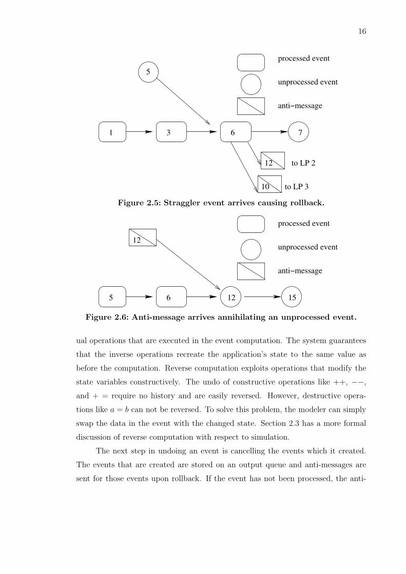
2.5 Straggler event arrives causing rollback. . . . . . . . . . . . . . . . . . . 16

2.6 Anti-message arrives annihilating an unprocessed event. . . . . . . . . . 16

2.7 Anti-message arrives causing secondary rollback. . . . . . . . . . . . . . 17

2.8 Transient message problem. . . . . . . . . . . . . . . . . . . . . . . . . . 18

2.9 Simultaneous message problem. . . . . . . . . . . . . . . . . . . . . . . 18

2.10 LP state to message data swap example. . . . . . . . . . . . . . . . . . 24

3.1 The topology of the model. . . . . . . . . . . . . . . . . . . . . . . . . . 34

3.2 Flow chart for request arrival and neighbors request. . . . . . . . . . . . 35

3.3 Flow chart for neighbor response and database request. . . . . . . . . . 36

3.4 Flow chart for client response. . . . . . . . . . . . . . . . . . . . . . . . 37

3.5 Flow chart for add view. . . . . . . . . . . . . . . . . . . . . . . . . . . 38

3.6 Forward and reverse CAVES request. . . . . . . . . . . . . . . . . . . . 44

3.7 Forward and Reverse CAVES response. . . . . . . . . . . . . . . . . . . 47

3.8 Reverse computation code without considering variable dependencies. . 50

3.9 Reverse computation code using variable dependencies. . . . . . . . . . 50

4.1 Forward and reverse of TCP correct ack . . . . . . . . . . . . . . . . . . 66

4.2 Forward and reverse of TCP updating cwnd . . . . . . . . . . . . . . . 68

4.3 Forward and reverse of TCP handling a duplicate ack . . . . . . . . . . 68

4.4 Forward and reverse of TCP process sequence number . . . . . . . . . . 70

viii

4.5 Comparison of SSFNet’s and ROSS’ TCP models based on sequencenumber for TCP Tahoe retransmission timeout behavior. Top panel isROSS and bottom panel is SSFNet. . . . . . . . . . . . . . . . . . . . . 71

4.6 Comparison of SSFNet and ROSS’ TCP models based on congestionwindow for TCP Tahoe retransmission timeout behavior test. Top panelis ROSS and bottom panel is SSFNet. . . . . . . . . . . . . . . . . . . . 72

4.7 Comparison of SSFNet’s and ROSS’ TCP models based on sequencenumber for TCP Tahoe fast retransmission behavior. Top panel is ROSSand bottom panel is SSFNet. . . . . . . . . . . . . . . . . . . . . . . . . 73

4.8 Comparison of SSFNet’s and ROSS’ TCP models based on congestionwindow for TCP Tahoe fast retransmission behavior test. Top panel isROSS and bottom panel is SSFNet. . . . . . . . . . . . . . . . . . . . . 74

4.9 AT&T Network Topology (AS 7118) from the Rocketfuel data bank forthe continental U.S. . . . . . . . . . . . . . . . . . . . . . . . . . . . . . 81

4.10 Campus Network [59]. . . . . . . . . . . . . . . . . . . . . . . . . . . . . 84

4.11 Ring of 10 Campus Networks [35]. . . . . . . . . . . . . . . . . . . . . . 85

4.12 Packet rate as a function of the number of processors. . . . . . . . . . . 86

5.1 New data structures added to ROSS for the Reverse Memory Subsystem. 93

5.2 Kernel Process Memory Buffers Fossil Collection Function. . . . . . . . 94

5.3 Freeing of an event after annihilation. . . . . . . . . . . . . . . . . . . . 95

5.4 Initialization Functions and Variables for the Reverse Memory Subsys-tem. . . . . . . . . . . . . . . . . . . . . . . . . . . . . . . . . . . . . . 96

5.5 The allocation function for the Reverse Memory Subsystem. . . . . . . 98

5.6 The reverse allocation function for the Reverse Memory Subsystem. . . 98

5.7 The free and reverse free functions for the Reverse Memory Subsystem. 99

5.8 The event memory set function for the Reverse Memory Subsystem. . . 100

5.9 The event memory get function for the Reverse Memory Subsystem. . 101

5.10 The reverse event memory get function for the Reverse Memory Sub-system. . . . . . . . . . . . . . . . . . . . . . . . . . . . . . . . . . . . 101

5.11 CAVES cache data structure. . . . . . . . . . . . . . . . . . . . . . . . . 107

5.12 CAVES removal of a view. . . . . . . . . . . . . . . . . . . . . . . . . . 108

ix

5.13 CAVES reverse computation code for a removal of a view. . . . . . . . . 109

5.14 CAVES allocation of a view. . . . . . . . . . . . . . . . . . . . . . . . . 109

5.15 CAVES reverse computation of a view allocation . . . . . . . . . . . . . 110

6.1 Multicast graphic from Cisco [21]. . . . . . . . . . . . . . . . . . . . . . 114

6.2 Memory Set Routine. This routine is performed when setting a memorybuffer to an event. B is the memory buffer. E is the event. . . . . . . . 117

6.3 Memory free routine. This routine is performed on all event allocations.B is the memory buffer. E is the event. . . . . . . . . . . . . . . . . . . 118

6.4 Additional Memory Required for Increases in Levels. . . . . . . . . . . . 119

6.5 Memory required with respect to shared data segment size. One case is8 multicast trees, 10 levels and 8 start events and the other case is 16trees, 10 levels and 4 start events. . . . . . . . . . . . . . . . . . . . . . 120

6.6 Event Rate with respect to shared data segment size. One case is 8multicast trees, 10 levels and 8 start events and the other case is 16trees, 10 levels and 4 start events . . . . . . . . . . . . . . . . . . . . . 121

x

AKNOWLEDGEMENTS

I would like to thank my adviser and my mentor Christopher Carothers for his

support and guidance that helped me through my graduate studies and along with

his belief and confidence in my abilities. I have an immense amount of gratitude

for the knowledge I gained from his council and guidance. I feel fortunate to have

Chris as my advisor, teacher and friend.

I want to express my gratitude to Shivkumar Kalyanaraman, Sibel Adali,

Boleslaw Szymanski and Biplab Sikdar for serving on my committee and helping

me with my dissertation. In addition Boleslaw Szymanski was kind enough to allow

me the usage of his cluster for performance results.

I would like to thank David Bauer for his help throughout college whether

it was a class project or research. I enjoyed our lengthy discussions where his

enthusiasm helped me spawn many new ideas and insights in both our research and

my life.

I appreciate the faculty and staff in the Computer Science Department at

Rensselaer Polytechnic Institute who offered me a great study and research environ-

ment. I would also like to thank my fellow students for their help in preparing for

the qualifiers and their comments on my rehearsals for my candidacy presentation

and dissertation defense.

A special thanks to my parents for their belief and support of me in whatever

I choose to pursue. I’m grateful for their patience and understanding.

xi

ABSTRACT

Modeling and simulation is a valuable tool in the analysis of large-scale networks

and computer systems. To tackle these complexities, conservative parallel simula-

tion is often employed as an approach to reduce the runtime. Optimistic simulation

has previously been viewed out of the performance envelop for such models. How-

ever, with the advent of a new technique called reverse computation the memory

requirements for benchmark models have been dramatically reduced.

In this thesis, we demonstrate the use of reverse computation for allowing large-

scale simulation models to achieve greater scalability and performance. The models

developed for this thesis consisted of network protocols and distributed computer

system applications.

Within these models, reverse computation was important in achieving per-

formance gains and dispelling views that optimistic techniques operate outside of

the performance envelope. These are the first real-world models to leverage reverse

computation and demonstrate its efficiency. Our TCP model executed at 5.5 mil-

lion packets per second which is 5.14 times greater then PDNS’ packet rate of 1.07

million for the same large-scale network scenario. This experiment was performed

across a distributed cluster of 32 nodes and executed on one processor per node.

Observations made from the creation of these models led to the development of

the reverse memory subsystem and the idea of shared event data. The contribution

of this subsystem is that it allows for easier implementation of models and allows for

the models to use dynamic memory. This subsystem permits for an overall reduction

of memory in simulation models as compared to models that work in statically “pre-

allocated” memory. The idea of shared event data works by decreasing the amount

of duplicate information in the event. Our experiments with shared event data show

significant memory reductions when there is a high degree of redundant data.

These contributions when taken together as a whole enable real-world large-

scale models to be efficiently developed and executed in an optimistic parallel sim-

ulation framework.

xii

CHAPTER 1

Introduction

This chapter focuses on the motivation for the research, illustrates the scope of this

thesis, presents the main contribution, and offers a outline for this thesis.

1.1 Motivation

Large-scale systems are difficult to understand due to their size and complexity.

Analytical models give quick solutions but often are constrained or use assumptions

that may not reflect realistic operating conditions. These simplifications in the

models can cause important results to be overlooked. Simulation, on the other

hand, can lead to new insights that analytical models might have missed.

Currently, the Internet is one such large-scale system and will continue un-

dergoing growth. In [22] it is reported that Internet data traffic is doubling each

year. During 1997, the Internet traffic was between 2,500 and 4,000 TB/month [22].

By year-end 2002, they estimated that the amount of Internet traffic was between

80,000 and 140,000 TB/month. RHK, Inc., a market research and consulting firm,

has estimates that also fall into this range [75, 91].

Pervasive devices such as VOIP capable mobile phones [54], wireless PDAs and

portable consumer electronics (ie. ipod [49], PSP [86]) are likely to increase wired

and wireless network data growth rates. Microsoft has just announced “MSN Video

Downloads, which will provide daily television programming, including video content

from MSNBC.com, Food Network, FOX Sports and IFILM Corp., for download to

Windows Mobile (TM)-based devices such as Portable Media Centers and select

Smartphones and Pocket PCs.” [67] With the introduction of these new multimedia

subscription services the growth rates could increase.

To address bandwidth allocation and congestion problems that arise as net-

work data transfer rates increase, researchers are proposing new overlay networks

1

2

that provide a high quality of service and a near lossless guarantee. However, the

central question raised by these new services is what impact will they have in the

large? To address these and other network engineering research questions, high-

performance simulation tools are required.

The predominate technique for analyzing network behavior is discrete-event

simulation. One such simulator is NS [74] which has flexibility and ease of use, but

is not adequate for simulating large-scale networks. Consider the following example

of a simple network with 512 source nodes connected by a duplex link to 512 sink

nodes with UDP packets traversing the link configured for drop-tail-queueing. NS

will allocate to this network almost 180MB of RAM. This simulation processes

events at a rate of approximately 1,000 per second. For large-scale networks, we

require almost 1,000 to 100,000 times greater performance. These computational

requirements are immense and are unobtainable on a single processor.

One might believe that with faster processors, any sequential simulator’s per-

formance will adequately scale, however the problem evolves with the increasing of

processor performance. For example mobile phones were only capable of sending

pictures or browsing the web, soon they will be creating VOIP traffic and be able to

view streaming video. [54, 67] To address these large-scale network engineering re-

search questions in a scalable, deterministic modeling framework, we believe parallel

and distributed simulation techniques are an enabling technology.

Current research for networking using parallel simulation is largely based on

conservative algorithms. For example, PDNS [94] is a parallel/distributed network

simulator that creates a federation of NS simulators. With conservative algorithms,

the simulation waits until it can guarantee no event will arrive in its simulated

time past prior to processing an event (i.e, is it ”safe” to execute an event). This

approach limits the parallelism that can be leveraged within a model. In addition

conservative simulations are limited based on the topology because simulated time

delays between network elements are used to compute the safe times. Changes

in the topology while challenging for parallel simulation algorithms, are after all

the heart of network engineering research questions. Optimistic simulation does

not explicitly use the network topology as part of its synchronization mechanism

3

and as well it relaxes the need for precise processing of events in strict time stamp

order. Optimistic simulation uses a detection and recover scheme to identify out of

order event processing and corrects these errors with rollbacks. In order to perform

a rollback, the simulation system requires additional memory (i.e. “optimistic”

memory). This mechanism for synchronization automatically uncovers the available

parallelism in a model. These attributes make a good case for using an optimistic

synchronization approach to parallel discrete-event simulation of large-scale, real-

world network and computer systems.

1.2 List of Terms

Throughout this thesis many different terms will be used. The core terms are

reverse computation, entropy, efficiency, event rate, and speedup and are defined as

followed:

• Reverse computation is realized by performing the inverse of the individ-

ual operations that are executed in the forward computation. The system

guarantees that the inverse operations recreate the application’s state to the

same value as before the computation. Reverse computation exploits opera-

tions that modify the state variables constructively. The undo of constructive

operations like ++, −−, and + = require no history and are easily reversed.

However, destructive operations like a = b can not be reversed.

• Entropy in a physical system is the measure of the amount of thermal energy

not available to do work. In a computational system, information in a message

is proportional to the amount of free energy required to reset the message to

zero. The act of resetting the message to zero uses energy and that used energy

is turn into heat (i.e., entropy). For our research here, we refer to entropy as

the amount of information loss within a system or a model that is part of

some sequential or multiprocessor execution. Destructive operations such as

an assignment or a copy lead to a great deal of entropy. However, reverse

computation on constructive operations is entropy free because the previous

value can always be recreated and thus no data lost. We also use entropy with

4

respect to caching. A cache with a higher miss rate is undergoing a higher

amount of entropy due to missed cache entries destroying the previous entries

in the cache. A better performing cache has less entries being replaced and

thus less entropy. Through out this thesis will be looking at ways of minimizing

the amount of entropy within models.

• Efficiency is defined as acting effectively with a minimum amount of expense

or unnecessary effort. We refer to the net events processed (i.e., excludes rolled

events) divided by the total number of events as efficiency because this value

represents the percentage of effective execution that our model performed.

We refer to our models as efficient due to the fact that they minimize memory

usage and execute effectively.

• Event rate is defined to be the total number of events processed less any

rolled back events divided by the execution time.

• Speedup is defined to be the event rate of the parallel case divided by event

rate of the sequential case. Because the total number of events are the same

between sequential and parallel runs of the same model configuration, this

definition is equivalent to using execution time. Speedup shows how effective

our parallel model executed. Event rate and Speedup are important because

they give us a way to compare our model and systems against others.

1.3 Scope of the thesis

The scope of this thesis is the investigation of large-scale optimistic parallel

discrete-event simulations on large-scale computing platforms and developing an

understanding of the fundamental limits of our discrete-event simulation engine in

the domain of large-scale network models and computer systems. In particular, the

study focuses on simulation of protocols and applications across the Internet. The

research can be broken down into three parts. The first part will discuss the design

of the models. The second part reveals the optimizations and methods dealing

with reverse computation. The third will discuss the implementation of additional

functionalities to the simulation system framework.

5

A breakdown of major research questions addressed by this thesis are:

• Model design is critical to the creation of efficient large-scale optimistic par-

allel simulation. What aspects of large-scale network models, as a motivating

example, can be exploited to improve performance without violating the need

for high-fidelity protocol dynamics?

• The models in large-scale optimistic simulations require large amounts of mem-

ory. State saving is a central overhead in event processing. How can we apply

reverse computation efficiently? What operations can be reversed to prevent

state saving?

• New functionalities are needed in the simulation system. What functionalities

can be added to increase ease of use along with minimizing memory usage?

What is the performance cost or benefit of such functionalities? Can these

new functionalities decrease the amount of memory needed?

This thesis will suggest and strive to answer these questions. Each area receives

equal focus and investigation.

1.4 Contributions

There are four major contributions of this thesis. The first contribution (Chap-

ters 3 and 4) is the development of efficient large-scale models in an optimistic

simulation framework. These models, include a transport layer protocol as well

as a database view storage system called CAVES. Our transport layer protocol

model simulates hosts sending and receiving files of given lengths across a realistic

network of routers using TCP which is describe later in Chapter 4. Our CAVES

model simulates a hierarchy of storage servers and databases which fulfill applica-

tions’ queries. Together they push the limits of the simulation engine and achieve

performance levels that were thought to be out of the scope of optimistic simula-

tion [111, 112, 113, 114]. In the design of these models, memory as well as processor

efficiency were the top priorities because they directly correlate with the model’s

execution time [17].

6

The second contribution (Chapters 3 and 4) is in the application of the meth-

ods of reverse computation which were employed in the construction process of

parallel models. The performance study demonstrates that the application of re-

verse computation to optimistic parallel simulation models decreases both space and

time complexity, thus enabling multi-dimensional scalability.

The third contribution (Chapter 5) is a new memory management approach

that is both easy to use as well as reduces model memory consumption. This is

accomplished by adding a reverse memory subsystem to the Rensselaer’s Optimistic

Simulation System (ROSS) API. Previously, all model memory management was

done “by hand”. This reverse memory subsystem decreases memory usage and

increases performance by decreasing the amount of “optimistic” memory required

by models.

The fourth contribution (Chapter 6) is in the development of shared event

data in an optimistic simulation. With this extension to the current framework

there will be a reduction in memory consumption which leads to greater scalability

in multicast network models.

These contributions when taken together as a whole enable real-world large-

scale models to be efficiently developed and executed in an optimistic parallel sim-

ulation framework.

1.5 Thesis Outline

The thesis is structured as follows:

Chapter 2 illustrates the history of simulation research which in turn intro-

duces the background for this thesis. An overview of both conservative and opti-

mistic parallel simulation synchronizations is given. This is followed by an assess-

ment of current research and concludes with applications of reverse computation.

In Chapter 3 presents the design and implementation of a configurable appli-

cation view storage system (CAVES). The CAVES model is comprised of a hierarchy

of view storage servers. The term view refers to the output or result of a query made

on the part of an application that is executing on a client machine. These queries

can be arbitrarily complex and formulated using SQL. The goal of this system is

7

to reduce the turnaround time of queries by exploiting locality both at the local

disk level as well as between clients and servers prior to making the request to the

highest level database server. We show the instrumentation of reverse computation

within the model and an analysis of the experimental data is performed and results

are presented.

Chapter 4 presents our TCP model which is comprised of hosts sending and

receiving files of given lengths across a realistic network of routers. The routers are

equipped with drop tail queues. This TCP model dispels the view that optimistic

simulation techniques operate outside the performance envelop for Internet protocols

and demonstrates that they are able to efficiently simulate large-scale TCP scenarios

for realistic networks.

Chapter 5 begins with a description of the reverse memory subsystem. The

reasons that led to the subsystem design are discussed. This is followed with an

explanation of its use along with example models. In addition there is a discussion

on how this subsystem eases model development. The chapter concludes with a

performance study which illustrates the subsystems benefits.

Chapter 6 explains shared event data. The chapter begins with an example

model which exhibits the properties where this new functionality would be most

useful. This is followed with a discussion of the challenges that arise from imple-

mentation in an optimistic simulation system. The chapter ends with a performance

analysis.

In Chapter 7 summarizes the current work and give conclusions for this re-

search.

CHAPTER 2

Related Work

This chapter illustrates the history of simulation research which in turn introduces

the background for this thesis. An overview of both conservative and optimistic

parallel simulation synchronization is given. This is then followed by a comparison of

the two synchronization techniques. Then the chapter discusses reverse computation

with respect to simulation and concludes with other uses of reverse computation.

2.1 Introduction to Simulation

Simulation is defined as “the imitation of the operation of a real-world process

or system over time.” [7] Computer simulation is a computation that models a

process or system and is beneficial because it is repeatable, controllable, sometimes

faster and less costly than the real system. Simulations allow for the study of com-

plex large-scale models that are intractable to closed-form mathematical methods

or analytic solutions.

The time flow mechanism allows a simulation model’s state to change while

time advances. There are two main classifications of the time flow mechanism,

continuous and discrete. Continuous simulation has the state changing continuously

over time. Some examples of continuous simulations are motion of vehicles and

global climatic models. For discrete simulation, the simulation model views time as

a set of discrete points in which state changes occur. There is a hybrid model which

combines the two time flow mechanisms [60].

Two of the most common types of discrete simulations are time-step and event-

driven. The time-step approach advances simulation time in small constant time

intervals. This approach gives the impression of continuous time and therefore might

be suitable for the simulation of some continuous systems.

Event-driven has time being advanced when “something interesting” occurs.

This “something interesting” is the event and is the key idea behind discrete-event

8

9

while( simulation executing )

{

remove event with the smallest time stamp from event-list

sim_time = time stamp of event

pass event to models event handler

}

Figure 2.1: Discrete-event simulation event processing loop.

simulations [33]. Some examples of discrete-events are airplanes taking off, landing,

and loading.

Discrete-event simulation contains algorithms for event management and an

executable software description of the model being simulated. Here, the model is

decomposed into “atomic” events. Each event has a time stamp of when it is to

occur and the events are stored in an event-list. The smallest event is removed from

the event-list and the simulation or “virtual” time is set to that event’s time stamp.

The event is then processed by the model when it is the smallest unprocessed event

in the system. Figure 2.1 shows the discrete-event processing loop.

The modeler can design a simulation with one of three world-views: event-

oriented, process-oriented, and activity-scanning. With event-oriented, the modeler

constructs event handlers and the event handlers on methods are called for the

specific event. This method is sometimes more difficult to construct models with,

but is the most efficient.

In the Process-oriented world view, the modeler can specify the model as a

collection of processes [33]. However, there is more overhead due to the thread man-

agement. Moreover, network protocols actually behave in an event-driven manner,

such as TCP. Thus, for the research domain here, the event-driven world-view is the

most appropriate.

The activity-scanning world-view is a variation on the time-step flow mecha-

nism. The simulation is a collection of procedures with a predicate associated with

10

each one. When each time-step occurs, the predicates are evaluated and if that

predicate is true the associated procedure is executed [33]. This world view is not

as efficient because of the predicate evaluation process.

2.2 Parallel Discrete-Event Simulation

Parallel discrete-event simulation is a well established field that has been ap-

plied to a diverse set of problems; from networking to air traffic control [109]. With

parallel discrete-event simulations, a single model is divided or distributed onto a

multiple processors. These processors could be tightly coupled in a single system

or distributed across a number of host systems and communicate over a high-speed

network. The end goal is typically the same: reduce the model’s overall execution

time. Time-critical applications and on-the-fly simulations have become realities.

In parallel discrete-event simulation individual physical processes are modeled

by logical processes (LPs). These processes communicate between each other with

time stamped events or messages.

The challenge for parallel discrete-event simulation is making sure events are

processed in correct time stamp order. An event processed at an earlier time could

effect the state of the simulation which is used for the processing of events at later

times. The causality constraint asserts that events are processed in time stamp

order and a causality error occurs when an event is processed out of order. If a

causality error transpires, the accuracy of the simulation will be questioned. The

local causality constraint states that all events within that LP must be processed in

nondecreasing time stamp order. All LPs adhering to the local causality constraint

guarantee the causality constraint for the entire simulation.

The correct local time stamp ordering of the events is difficult in parallel

simulation because there is no notion of a global simulation time clock. An example

of a causality error in a simple parallel simulation of an airport model is shown in

Figure 2.2. Here, two airports are modeled as LPs, each being mapped on a different

processor. The first airport has a plane departing at time 3. The second airport

has a plane loading at time 7. Both processors execute their events concurrently.

The plane departing, creates an arrival event at the second airport at time 6. The

11

0 3 6 7

2

1

airport processed event

unprocessed event

Simulation Time

Figure 2.2: Causality error.

processing of the arrival at time 6 would result in the causality constraint being

violated.

In order to prevent causality errors there is a need for a synchronization method

between processors or computers. There are two categories of synchronization meth-

ods: conservative and optimistic. Conservative synchronization makes sure it is safe

to execute an event. Here, the local causality constraint is strictly enforced. Op-

timistic synchronization, on the other hand, relaxes the local causality constraint.

This allows for causality errors to occur as long as they are later corrected. Rolling

back of events incorrectly processed and other recovery methods must be incorpo-

rated into the optimistic simulation system.

2.2.1 Conservation Synchronization

Conservative synchronization makes sure it is safe to execute an event. The

first conservative algorithm was the Chandy/Misra/Bryant CMB, named after the

creators. The algorithm makes sure it is safe to execute and uses null messages to

avoid deadlock [11, 18].

The CMB algorithm has logical processes connected by directional links. The

LP communicates across these links by sending messages. In the LP there is a

queue for each incoming link. The three assumptions that must hold true for the

12

waiting on 3

15, 10

Aiport 1

waiting on

waiting on1

2

Airport 2

11

8

5

17, 13

Airport 3

25

Figure 2.3: Deadlock cause by a waiting cycle.

Chandy/Misra/Bryant algorithm are:

• Time stamp messages sent over a link must be sent in nondecreasing order.

• The communication network, the link, must guarantee that messages are re-

ceived in the same order they are sent.

• The transfer of messages must be reliable (i.e., no losses).

Based on these constraints it is not possible for a smaller time stamped message

to arrive on an incoming link than previously received. Each link’s queue has a clock

value associated with it. The clock value is the smallest time stamped message on

the queue. If the queue is empty, the clock value is the last time stamped message

processed from that queue. The queue with the smallest clock value is checked. If

there are messages in that queue, the smallest time stamped message is processed.

13

If the queue is empty the LP waits for a message to arrive on that link. The “wait”

property of the algorithm enables a deadlock condition to be possible. Figure 2.3

illustrates a deadlock case.

The CMB algorithm accounts for this possibility of deadlock by having null

messages. A null message is sent after the processing of each message. The null

message has no information needed for the model. They only contain a time stamp

guaranteeing that no message will arrive from the sender LP with a time stamp less

than the sent time stamp. The LP receiving the null message can advance the clock

value based on the null message which in turn allows for safe event processing and

makes time advancement possible. In the null message the lookahead is included in

the time stamp. “Lookahead refers to the ability to predict what will happen, or

more importantly, what will not happen, in the simulated future.” [32] With this

knowledge the lookahead included in the time stamp is the amount of simulation

time that an LP can predict into the simulated future. The lookahead has to be

derived from the model based-on limitations on how quickly physical processes can

interact. It is believed that poor lookahead in a model “results in more frequent

synchronizations, therefore, higher overheads”. [60] In models with zero lookahead

deadlock is still possible.

Demand-driven is an alternative to the null message approach. Demand-driven

has the blocked LP and requests the next time stamp from that link. Once the

response is returned, the LP can continue execution. This method reduces the

message overhead created by the null messages but increases delay because of the

two transmissions.

The CMB algorithm is a deadlock avoidance algorithm. There are other con-

servative algorithms that focus on deadlock detection and recovery. [19, 68] Deadlock

can be overcome by exploiting the knowledge that the smallest time stamped event

in the system can be processed. Deadlock detection algorithms can allow for zero

lookahead cycles in simulations, however, “they tend to be overly conservative” and

parallelism is limited. [60]

The Critical Channel Traversing (CCT) algorithm extends the CMB algorithm

with the addition of policies that determine when an LP should be scheduled to

14

3 6 71

5

unprocessed event

processed event

Figure 2.4: Straggler event arrives

execute events. The CCT algorithm schedules the LPs with the largest number of

events that are ready to execute by identifying critical channels in the model [110].

The most recent conservative synchronization algorithm was Nicol’s composite

synchronization [72]. This scheme utilizes a barrier synchronization approach for

those LPs that are “far apart” in virtual time and Critical Channel Traversing

for LPs that are more closely related in virtual time. This algorithm effectively

divides LPs into these two categories based on an optimal algorithm. The composite

synchronization avoids channel scanning limitations associated CCT while at the

same time reducing the frequency of applying global barriers. Thus, it minimizes

the overheads of both CCT and barrier synchronization mechanisms.

2.2.2 Optimistic Synchronization

Optimistic synchronization allows for execution to happen as fast as possible

(i.e., synchronization or wait-free) assuming there are no causality errors. A wait-

free implementation guarantees that any process can complete any operation in a

finite number of steps, regardless of the execution speeds on the other processes [44].

If an error occurs the simulator provides mechanisms for detecting it and correcting

the error. The first optimistic synchronization algorithm was Time Warp done by

Jefferson [51]. The Time Warp algorithm is composed of two pieces, the local control

mechanism and the global control mechanism.

The local control mechanism acts in each LP and is largely independent from

other LPs. An LP after processing an event, inserts it into a processed event queue.

The processed event queue is used for reprocessing that is caused by a rollback. A

15

rollback happens when a straggler message arrives at the LP. This can be seen in

Figure 2.4. In order to maintain the local causality constraint, changes to the LP’s

state caused by out of order processing must be undone or rolled back. Once the

LP state is corrected the straggler message can be processed and the other events

then can be re-executed, thus maintaining the local causality constraint.

In the undo process there needs to be ways of reversing the state changes

and canceling events that were incorrectly sent. Methods of undoing state changes

include: Copy state saving, infrequent state saving [9, 56, 57], incremental state

saving [10, 41, 95, 100, 108], and reverse computation [15, 16, 80].

Copy state saving, copies all changeable variables in the state before each

event gets processed. When a straggler message arrives, the LP knows the exact

construction of the previous state. This method requires sufficient memory since a

full copy of the LPs state is required.

Infrequent state saving is similar to copy state saving but only copies the

state at intervals. When a straggler message arrives, the LP rolls back to a state

before the straggler. The LP then re-executes all events up to the desired state.

The re-executing of events is called “coasting forward”. [31] During this “coasting

forward” the re-executed events abstain from resending or canceling events since it

is unnecessary. This method reduces the memory required but adds the overhead

of the coasting forward phase.

Incremental state saving only saves the variables that where modified by the

current event. One form keeps a log of which variables were modified. When the

LP rolls back, the simulator is required to browse the log in decreasing time stamp

order to correctly revert the state changes. This form of incremental state saving

can be implemented by the modeler. Other forms try to automate the process. One

such form has been implemented by overloading assignment operators in C++. The

overloading of operators makes the state saving transparent to the user [95]. In

[108] incremental state saving was implemented by automatically editing compiled

executable code. Incremental state saving is useful when few state variables are

modified per event processed.

Finally reverse computation is realized by performing the inverse of the individ-

16

3 6 71

5

12 to LP 2

to LP 310

processed event

unprocessed event

anti−message

Figure 2.5: Straggler event arrives causing rollback.

65 12 15

anti−message

unprocessed event

processed event

12

Figure 2.6: Anti-message arrives annihilating an unprocessed event.

ual operations that are executed in the event computation. The system guarantees

that the inverse operations recreate the application’s state to the same value as

before the computation. Reverse computation exploits operations that modify the

state variables constructively. The undo of constructive operations like ++, −−,

and + = require no history and are easily reversed. However, destructive opera-

tions like a = b can not be reversed. To solve this problem, the modeler can simply

swap the data in the event with the changed state. Section 2.3 has a more formal

discussion of reverse computation with respect to simulation.

The next step in undoing an event is cancelling the events which it created.

The events that are created are stored on an output queue and anti-messages are

sent for those events upon rollback. If the event has not been processed, the anti-

17

13 15

12109 17

anti−message

unprocessed event

processed event10

Figure 2.7: Anti-message arrives causing secondary rollback.

message will annihilate that event. However, if the event has been processed by

the destination processor the anti-message will cause that event to be rolled back.

This is known as a secondary rollback. Figure 2.5 shows LP 1 receiving a straggler

message and sending the appropriate anti-messages. In Figure 2.6, the anti-message

is received before the event is processed and the event is annihilated. However, in

Figure 2.7 the anti-message is received after the event is processed and causes a

secondary rollback.

Another form of cancellation is Lazy Cancellation. This technique avoids

cancelling messages that will be later recreated. Lazy Cancellation only sends anti-

messages when the original message will not be created by event reprocessing [33].

The local control mechanism ensures that events are processed in time stamp

order which maintains the causality constraint. However, the memory required for

keeping processed events and state history is tremendous, if they are never reclaimed.

Thus there is a need for a memory garbage collection. The global control mechanism

takes care of these issues by determining a minimum time stamp for any future

rollback. This minimum time stamp is referred to as Global Virtual Time GVT.

Since GVT is the lowest time that the simulator can rollback to, all processed events

and I/O with a time less than GVT can be reclaimed and committed. The reclaiming

of memory used by processed events and state history is called fossil collection.

GVT requires the minimum time stamp over all unprocessed events or par-

18

B

A

15

2520Controller

Figure 2.8: Transient message problem.

B

A

25 20

15

Controller

Figure 2.9: Simultaneous message problem.

tially. There are two problems in obtaining this value. The first problem comes from

the fact that a message might be in transit while the processors are reporting their

minimum time stamp. This is called the transient message problem and is illustrated

in Figure 2.8. One solution to this problem is to have the receiver acknowledge the

message. Under this scheme, the sender is responsible for reporting the message in

a GVT computation until it receives the acknowledgment. This insures no transient

messages “fall between the cracks”. [33] However, if the receiver already performs

a GVT computation before the message arrives and the sender performs the GVT

computation after it is sent, both processors assume the message is accounted for by

the other. This problem is shown in Figure 2.9 and is referred to as the simultaneous

reporting problem.

Samadi’s algorithm fixes these problems by having the acknowledgment tagged

19

when it is sent between the period of a reported local minimum and a receiving new

GVT value [96]. These acknowledgments identify the ones that might “fall between

the cracks” [33] and now the sender will know to account for them. Mattern’s

GVT algorithm does not require message acknowledgments and uses the distributed

system concept of consistent cuts to calculate GVT [65]. Fujimoto’s GVT algorithm

exploits shared memory and greatly simplifies the GVT algorithm by generating a

cut by setting a global flag [34].

Once GVT is calculated the fossil collection can occur. This typically is done in

a batch mode. All processed events with a time stamp less than GVT are reclaimed

and placed into a free list from which internal events are allocated from.

2.2.3 Comparison between Optimistic and Conservative Synchroniza-

tion

The debate between which synchronization approach is superior has contin-

ued for years. There is no overall winner. Conservative has its advantage over

optimistic and vice-versa. In this subsection those advantages and disadvantages

will be discussed.

Optimistic synchronization can fully exploit parallelism and is only limited by

the actual dependencies. Whereas the conservative approach is limited by potential

dependencies. Optimistic synchronization can be viewed as more difficult to design

and construct models. The modeler has to be concerned with state saving or the

reverse computation code. A solution to this problem is to employ code translation

and generation techniques such as those used by Perumalla [80, 81]. However,

dynamic memory usage has been viewed as being difficult and is often avoided.

With the implementation of the reverse memory subsystem, these problems are

eased.

Conservative models do not have to handle inconsistencies due to lagging roll-

backs and stale state that can occur in optimistic synchronization [73]. However,

they need to design their models with explicit parallelism. With optimistic syn-

chronization parallelism is automatically exploited. Conservative synchronization

in addition has a limited model space due to lack of lookahead [58]. Conservative

20

models with good lookahead have an advantage over optimistic ones because they do

not have to perform rollbacks and they have a smaller memory footprint. However,

conservative synchronization has difficulties in dealing with dynamic topologies.

There is clearly no distinct winner. The best synchronization approach is

mainly model dependent. However, optimistic protocols might have the upper-hand

considering their ability to handle models with little lookaheads. Some of the more

interesting Internet models have small lookaheads such as ad-hoc wireless networks,

networks with low delays and dynamically changing topologies (i.e., link and route

changes) [2, 79, 103].

2.3 Reverse Computation

In optimistic simulation systems [51], the most common technique for realizing

rollback is state saving. In this technique, the original value of the state is saved

before it is modified by the event computation. Upon rollback, the state is restored

by copying back the saved value. An alternative technique for realizing rollback is

reverse computation [15, 16, 80]. In this technique, rollback is realized by performing

the inverse of the individual operations that are executed in the event computation.

The system guarantees that the inverse operations recreate the application’s state

to the same value as before the computation.

The key property that reverse computation exploits is that a majority of the

operations that modify the state variables are “constructive” in nature. That is,

the undo operation for such operations requires no history. Only the most current

values of the variables are required to undo the operation. For example, operators

such as ++, −−, + =, − =, ∗ = and / = belong to this category. Note, that

the ∗ = and / = operators require special treatment in the case of multiplying or

dividing by zero, and overflow/underflow conditions. More complex operations such

as circular shift (swap being a special case), and certain classes of random number

generation also belong here.

Operations of the form a = b, modulo and bitwise computations that result in

the loss of data are termed to be destructive. Typically these operations can only

be restored using conventional state saving techniques. Table 2.1 show the rules

21

Type Description Application Code Bit Requirements

Original Instrumented Reverse Self Child Total

T0 simple choice if()s1;elses2;

if(){s1;b=1;}else{s2;b=0;}

if(b==1){inv(s1);}else{inv(s2);}

1 x1, x2 1 +max(x1, x2)

T1 compoundchoice (n-way)

if()s1;elsif()s2;elsif()s3;else()sn;

if() {s1;b=1;}elsif(){s2;b=2;}elsif(){s3;b=3;}else {sn;b=n;}

if(b==1){inv(s1);}elsif(b==2){inv(s2);}elsif(b==3){inv(s3);}else{inv(sn);}

lg(n) x1, x2,..., xn

lg(n)+max(x1, ...xn)

T2 fixed itera-tions (n)

for(n)s;

for(n)s;

for(n)inv(s);

0 x n ∗ x

T3 variable iter-ations (maxi-mum n)

while()s;

b=0;while(){s;b++;}

for(b)inv(s);

lg(n) x lg(n) +n ∗ x

T4 function call foo(); foo(); inv(foo)(); 0 x xT5 constructive

assignmentv@ =w;

v@ =w;

v =@w;

0 0 0

T6 k-byte de-structiveassignment

v =w;

{b =v; v =w; }

v = b; 8k 0 8k

T7 sequence s1;s2;sn;

s1;s2;sn;

inv(sn);inv(s2);inv(s1);

0 x1+... +xn

x1 + ...+ xn

T8 jump (labellbl as targetof n goto’s)

gotolbl;s1;gotolbl;sn;lbl:s;

b=1;goto lbl;s1;b=n;goto lbl;sn;b=0;label:s;

inv(s);switch(b){case 1:gotolabel1;case n:gotolabeln;}inv(sn);labeln:inv(s1);label1:

lg(n+1)

0 lg(n +1)

T9 Nestings ofT0-T8

Apply the above recursively Apply the above recursively

Table 2.1: Summary of treatment of various statement types.Generation rules and upper bounds on state size requirements for supporting reverse com-putation. s, or s1..sn are any of the statements of types T0..T7. inv(s) is the correspondingreverse code of the statement s. b is the corresponding state saved bits “belonging” tothe given statement. The operator = @ is the inverse operator of a constructive operator@ =, (e.g., + = for − =) [16].

that can be recursively applied to forward computation code that will generate the

reverse code. The significant parts of these rules are their state bit size requirements,

22

and the reuse of the state bits for mutually exclusive code segments. We explain

each of the rules in detail next.

• T0: The if statement can be reversed by keeping track of which branch is

executed in the forward computation. This is done using a single bit variable,

which is set to 1 or 0 depending on whether the predicate evaluated to true

or false in the forward computation. The reverse code can then use the value

of the bit to decide whether to reverse the if part or the else part when trying

to reverse the if statement.

The bodies of the if part and the else part are executed mutually exclusively,

the state bits used for one part can also be used for the other part. Thus, the

state bit size required for the if statement is one plus the larger of the state

bit sizes, x1, of the if part and x2 of the else part, i.e., 1 + max(x1, x2).

• T1: Similar to the simple if statement (T0), an n-way if statement can be

handled using a variable b of size lg(n) bits. The state size of the entire if

statement is lg(n) for b, plus the largest of the state bit sizes, x1 . . . xn, of the

component bodies, i.e., lg(n) + max(x1 . . . xn) (since the component bodies

are all mutually exclusive).

• T2: An n iteration loop, such as a for statement, whose body requires x state

bits for reversibility. Then n instances of the x bits can be used to keep track

of the n instances of the body, giving a total of n ∗ x bit requirement for the

loop statement. The inverse of the body is invoked n times in order to reverse

the loop.

• T3: Consider a loop with variable number of iterations, such as a while state-

ment. This statement can be treated the same as a fixed iteration loop, but

the actual number of iterations executed can be noted at runtime in a variable

b. The state bits for the body can be allocated based on an upper bound n on

the number of iterations. Thus, the total state size added for the statement is

lg(n) + n ∗ x.

23

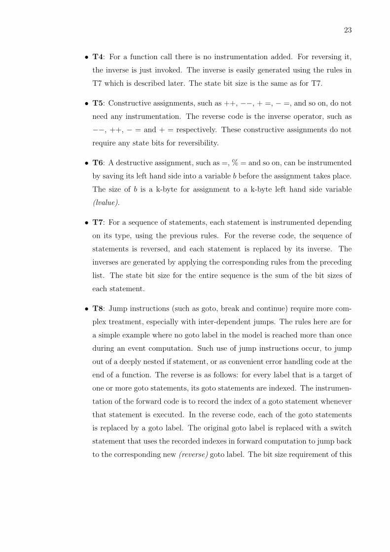
• T4: For a function call there is no instrumentation added. For reversing it,

the inverse is just invoked. The inverse is easily generated using the rules in

T7 which is described later. The state bit size is the same as for T7.

• T5: Constructive assignments, such as ++, −−, + =, − =, and so on, do not

need any instrumentation. The reverse code is the inverse operator, such as

−−, ++, − = and + = respectively. These constructive assignments do not

require any state bits for reversibility.

• T6: A destructive assignment, such as =, % = and so on, can be instrumented

by saving its left hand side into a variable b before the assignment takes place.

The size of b is a k-byte for assignment to a k-byte left hand side variable

(lvalue).

• T7: For a sequence of statements, each statement is instrumented depending

on its type, using the previous rules. For the reverse code, the sequence of

statements is reversed, and each statement is replaced by its inverse. The

inverses are generated by applying the corresponding rules from the preceding

list. The state bit size for the entire sequence is the sum of the bit sizes of

each statement.

• T8: Jump instructions (such as goto, break and continue) require more com-

plex treatment, especially with inter-dependent jumps. The rules here are for

a simple example where no goto label in the model is reached more than once

during an event computation. Such use of jump instructions occur, to jump

out of a deeply nested if statement, or as convenient error handling code at the

end of a function. The reverse is as follows: for every label that is a target of

one or more goto statements, its goto statements are indexed. The instrumen-

tation of the forward code is to record the index of a goto statement whenever

that statement is executed. In the reverse code, each of the goto statements

is replaced by a goto label. The original goto label is replaced with a switch

statement that uses the recorded indexes in forward computation to jump back

to the corresponding new (reverse) goto label. The bit size requirement of this

24

Forward

1. temp = SV->b;

2. SV->b = M->b + 5;

3. M->b = temp;

Reverse

1: temp = M->b;

2. M->ack = SV->b - 5;

3. SV->b = temp;

Figure 2.10: LP state to message data swap example.

scheme is lg(n) where n is the number of goto statements that are the sources

of that single target label.

• T9: Any legal nesting of the previous types of statements can be treated by

recursively applying the generation rules [16].

In Sections 3.3.2 and 4.3.3 shows the application of these rules on pseudo code

for the CAVES and TCP models.

The rules in Table 2.1 merely show the bit requirement upper bounds on

particular programmatic constructs. We can however, break the rules without loss

of correctness or model accuracy and achieve greater efficiency . First lets consider

a simple optimization involving the swap operation. We observe that many of these

destructive operations are a consequence of the arrival of data contained within the

event being processed. For example, a message changes the state of a model. With

conventional state saving, we would have to have an additional variable to save the

old variables value. However, to solve this problem, one can simply swap the data

in the event with the changed state of the logical process (LP). This swap is shown

in Figure 2.10. In that figure and throughout this chapter the state is represented

by the variable SV and the message variable will be M. When the event is rolled

back, the event data and LP data are just re-swapped.

25

The above solution works well as long as there is a one-to-one mapping between

message data and the amount of LP state being modified. However, as we observed

in our CAVES model, this is not always the case. It may come to pass that a message

may cause the deletion or destruction of data that is too large to be swapped into

the message. An example of this and a possible solution is shown in Section 3.3.3.

Kalyan Perumalla and Richard Fujimoto have implemented a reverse C com-

piler called RCC which takes C code and creates reversible code [81]. RCC does

not support swaps and has its other limitations. However, the reverse C compiler

is a good start for easing the generation of reverse code. In order to generate code

which performs close to hand written reverse code, the user code must be riddled

with pragmas. RCC gives the user the ability to define their own reverse functions,

however they must have the same number of parameters as the forward functions

and be of the return type of void. This is not always the correct format for the

reverse functions. For example list operations such as push and pop are inverses.

These functions have different parameters and return types and therefore could not

be used as reverse functions for each other. In addition there is no functional-

ity for handling dynamic memory operations which are often required for models.

An excellent addition to the RCC would be the integration of our reverse memory

subsystem.

2.4 Other Applications of Reverse Computation and Opti-

mistic Execution

There has been a significant amount of other research done in the field of

reverse computation. Such research has been done in debugging applications, data-

base transactions, architectures and error detection and recovery. Each of these

areas differs from our area but provides insight on reverse computation.

There has been much research in debugging applications using reverse com-

putation. The main reason for this is to give the user a more intuitive away of

debugging. The common way of debugging is to put a breakpoint where the error

might have occurred and then reexecute the program until the breakpoint is reached.

If the error happens before the breakpoint the user must reexecute the program again

26

with a higher breakpoint point. If the program is quite lengthy this process could

take a significant amount of time. It has been observed that programmers some-

times spend up to 50% of their time debugging [4]. With reverse computation in

debugging, upon encountering a bug, the user can backtrack in the program with-

out reexecuting it, there by saving time and making the debugging more intuitive.

PROVIDE [69] uses a process history database to store process state changes. This

process history could take a large amount of memory and is often viewed unrealistic

for certain applications. IGOR [30] uses checkpointing and an interpreter to execute

forward till the specific program point is reached. This is similar to the infrequent

state saving used in optimistic simulation which is discussed in [9, 56, 57]. The

interpreters forward execution can be around 100 times slower so the checkpoint

interval is an important parameter. EXDAMS was an interactive debugger that has

a replay facility. It can only replay a programs execution. Changes can not be made

during the course of the playback [6]. Agrawal, DeMillo and Spafford in [3] use

structured backtracking to reduce the memory required. With this method, state

is only saved at the beginning and at the end of the structures. The user can not

reverse compute to the middle of a loop. They must go to the beginning of the loop

and step through it till they arrive at the middle.

Database transaction processing can use reverse computation or compensat-

ing operations when dealing with concurrency control. Two transactions can both

access the same abstract item as long as the transactions’ operations are backwards-

commutable. With the property of being backward-commutable the compensat-

ing operation can be performed and the transaction schedule will appear as if the

aborted transaction never happened. This type of schedule is said to be reducible

and hence recoverable. An example of two operations that are compensating would

be a withdraw and a deposit. For reference, compensating operations are applied

in reverse order to how they first appeared [55]. This is similar to how the inverse

operations are applied in our models.

Reversible computing has also been an interesting area of research. Within this

field of study, reversible logic and energy-efficient computation are investigated. It is

known that when changing from one state to an other state in irreversible computing

27

heat is dissipated. This entropy, “burns up your lap, runs up your electric bill, and

limits your computer’s performance.” [38] Away to overcome this limit is by using

reversible computing, which uncomputes bits rather than overwriting them. Un-

computing allows energy to be recovered and recycled for later use.“Unfortunately,

present-day oscillator technologies do not yet provide high enough quality factors to

allow reversible computing to be practical today for general-purpose digital logic,

given its overheads.” [38]

Pendulum is an implementation of a reversible architecture and was developed

by a group at MIT [105, 106]. R is a reversible programming language developed for

the pendulum architecture. The language R provides the functionalities of reversing

function calls using the rcall method [36]. This language is in its early stages and

does not support destructive operations.

Another reversible language is Janus which was constructed for the DEC

SYSTEM-20. This language provides a similar reverse method named UNCALL.

Janus is considered to be a throw-away piece of code [63].

Reverse computing can also be used to determine errors within computations.

The program executes forward until completion and then executes in the reverse.

If the final state of the reverse execution is different from the start state, an error

occurred and the result is untrustworthy. Reverse computation can also allow re-

covery from malicious attacks. The system can be reversed to a state before the

attack [37].

The idea of optimistic processing for database concurrency control has been

researched [42, 52, 53, 55]. Concurrency control prevents conflicts among transac-

tions such that their serializability can be guaranteed. “A system of concurrent

transactions is said to be serializable or has the property of serial equivalence if

there exists at least one serial schedule of execution leading to the same results for

every transaction and to the same final state of the database.” [42]

The optimistic concurrency control discussed in [53] has three phases. The

first being the read phase were only read operations are performed on the database

and the writes are subject to validation. Writes are performed on local copies of

data. The second phase is the validation phase were conflicts are discovered. Upon

28

discovery of a conflict the transaction is aborted and restarted. With a successful

validation the local copies are made global in the write phase.

With optimistic concurrency control deadlock is not possible. However there is

a chance for starvation, and when a starving process is observed it can be guaranteed

execution by restarting the process without releasing the critical section semaphore.

This is equivalent to write locking the entire database [53].

Due to the storage overheads, optimistic concurrency control restricts itself

to rather short writer transactions [42]. However, for query-dominant transactions

systems optimistic concurrency control appears ideal because the validation is often

trivial and parallelism can be exploited.

Another form of optimistic concurrency control has been proposed using the

Time Warp mechanism [52]. Time Warp is the mechanism which we use in our sim-

ulation system. Within this type of concurrency control, transactions and data are

represented as objects or LPs. Communication is facilitated through message pass-

ing. Each transaction is given a unique time stamp and accesses to the data objects

must be performed in time stamp order. When out of order processing is observed,

a rollback is performed and forward execution continues. Within this method errors

only cause partial reprocessing of transactions instead of entire reprocessing.

Concurrency controls using locks are the more common types of concurrency

control. These types are similar to conservative simulations because they avoid all

possible conflicts, however sacrifice some degree of parallelism.

2.5 Chapter Summary

In this chapter we gave an introduction to different types of simulations. We

focused on parallel discrete-event simulation and discussed the different synchroniza-

tion approaches, conservative and optimistic. Conservative synchronization does not

need handling for causality errors and can be viewed as simpler to develop mod-

els. Conservative is limited by the lookahead that can be exploited from the model

whereas optimistic synchronization uses all possible parallelism. In addition we dis-

cussed reversible computation with respect to simulation. We presented rules for

generating reverse code for models as well as discussing the significance of applying

29

these rules cautiously. We concluded the chapter with a brief summary of other

applications of reverse computation.

CHAPTER 3

Configurable Application View Storage System:

CAVES

The CAVES model is a hierarchy of view storage servers. The term view refers to

the output or result of a query made on the part of an application that is executing

on a client machine. These queries can be arbitrarily complex and formulated using

SQL. The goal of this system is to reduce the turnaround time of queries by exploit-

ing locality both at the local disk level as well as between clients and servers prior

to making the request to the highest level database server. One interesting imple-

mentation problem is how to simulate the caches without using dynamic memory

allocations.

This model has been designed for execution with an optimistic parallel simu-

lation engine. As previously discussed, one of the primary drawbacks of this parallel

synchronization mechanism has been high overheads due to state saving. We ad-

dressed this problem by implementing the models using reverse computation when

possible.

The chapter begins with a discussion of Rensselaer’s Optimistic Simulation

System’s (ROSS’) data structures and then a CAVES model overview is presented

in Section 3.2. It is then followed with the event flow diagrams and a discussion in

Section 3.2.4. The implementation of CAVES atop the ROSS engine is presented in

Section 3.2.5. Then, there is a discussion of the reverse computation code for the

CAVES model in Section 3.3.2. The chapter concludes with a performance study of

the model.

3.1 ROSS’ Data Structures

ROSS’ data structures are organized in a bottom-up hierarchy. Here, the core

data structure is the tw event. Inside every tw event is a pointer to its source and

30

31

destination LP structure, tw lp. Observe, that a pointer and not an index is used.

Thus, during the processing of an event, to access its source LP and destination LP

data only the following accesses are required:

my source lp = event− > src lp;

my destination lp = event− > dest lp;

Additionally, inside every tw lp is a pointer to the owning processor structure,

tw pe. So, to access processor specific data from an event the following operation is

performed:

my owning processor = event− > dest lp− > pe;

This bottom-up approach reduces access overheads and may improve locality

and processor cache performance [12, 13].

ROSS also uses a memory-based approach to throttle execution and safeguard

against over-optimism. Each processor allocates a single free-list of memory buffers.

When a processor’s free-list is empty, the currently processed event is aborted and

a GVT calculation is immediately initiated. Unlike the Georgia Tech Time Warp

(GTW) simulation system [34], ROSS fossil collects buffers from each LP’s processed

event-list after each GVT computation and places those buffers back in the owning

processor’s free-list.

A Kernel Process is a shared data structure among a collection of LPs that

manages the processed event-list for those LPs as a single, continuous list. The net

effect of this approach is that the tw scheduler function executes forward on an

LP by LP basis, but rollbacks and more importantly fossil collects on a KP by KP

basis. Because KPs are much fewer in number than LPs, fossil collection overheads

are dramatically reduced.

The consequence of this design modification is that all rollback and fossil

collection functionality are shifted from LPs to KPs. To effect this change, a new

32

data structure was created, called tw kp. This data structure contains the following

items: (i) identification field, (ii) pointer to the owning processor structure, tw pe,

(iii) head and tail pointers to the shared processed event-list and (iv) KP specific

rollback and event processing statistics.

When an event is processed, it is threaded into the processed event-list for a

shared KP. Because the LPs for any one KP are all mapped to the same processor,

mutual exclusion to a KP’s data can be guaranteed without locks or semaphores.

In addition to decreasing fossil collection overheads, this approach reduces memory

utilization by sharing the above data items across a group of LPs. For a large con-

figuration of LPs (i.e., millions), this reduction in memory can be quite significant.

Experimental analysis suggests a typical KP will service between 16 to 256 LPs,

depending on the number of LPs in the system. Mapping of LPs to KPs is accom-

plished by creating sub-partitions within a collection of LPs that would be mapped

to a particular processor.

While this approach appears to have a number of advantages over either “on-

the-fly” fossil collection [34] or standard LP-based fossil collection, a potential draw-

back with this approach is that “false rollbacks” would degrade performance. A

“false rollback” occurs when an LP or group of LPs is “falsely” rolled back because

another LP that shares the same KP is being rolled back. This phenomenon was

not observed in the PCS model [12].

3.2 CAVES Model

3.2.1 CAVES Model Overview

CAVES is a configurable applications view storage system. This system in

practice is designed to work as a middle-ware system, connecting multiple possibil-

ities of distributed servers to multiple possibilities of distributed clients. The main

purpose of any storage system is to reduce the overall turnaround time between

an application and a data provider. To achieve this, storage systems make use of

the possible locality between different data requests and try to optimize the overall

performance by storing data that is most likely to be re-requested in the near future

in a fast storage medium. In this storage system, we consider the local disk of a

33

storage management system as a fast medium compared to networked and possibly

distant servers that process complex database queries. We use view to refer to the

output of a query in any application.

Examples of applications that involve costly queries include data warehousing

and data mining applications that process complex queries over large data sets,

applications that use spatial aggregations and correlations over complex vector data,

biological databases that process highly complex sequence comparison algorithms,

and large data sets obtained from scientific experiments. In such applications, the

time to process and transmit a single query may be rather high even in the presence

of indices and the size of the output may be very large. The cost of producing

such a data set might be much larger than the cost of writing and reading back the

data set from the local disk. In regular storage replacement algorithms, the goal

of the system is to optimize the total number of hits. This assumes that the cost

of producing each item in the storage is uniform. However, this is not the case for

complex queries that are transmitted over a network which optimizes the overall

savings in time. As a result, the replacement policies for an application may vary

greatly based on its workload.

3.2.2 CAVES Server

A CAVES Server is comprised of a view storage and corresponding statistics.

The view storage is sorted by the priorities of the views. The view with the lowest

priority is at the head of the storage and will be the first to be removed when space

is needed to insert a new view. A view’s priority is calculated by its properties

and other external information, such as network speed and disk speed. The view

priorities are a very important part of the real CAVES system because they affect

which views are stored, which impacts the overall savings that the CAVES system

can offer.

The CAVES server receives requests for views. If the view is in its storage,

the CAVES server will return the view. Otherwise it will request the view from

elsewhere. The CAVES server also receives returns of views. A returned view is

inserted into the storage if the entry criteria is met.

34

... ...

DatabaseDatabase

Middleserver

Middleserver

Middleserver

Middleserver

Client Client Client Client

... ... ...

Client

Figure 3.1: The topology of the model.

3.2.3 CAVES Hierarchy

The CAVES model is constructed from an idea of developing a CAVES Hier-

archy. The hierarchy offers a larger global storage of views than could have been

achieved with a single CAVES Server. The larger global storage allows for increased

time savings for the users of the real system.

The CAVES Hierarchy, as shown in Figure 3.1, is comprised of three types of

servers: client storage, middle storage and database. The client and middle storage

servers are CAVES Servers. The database servers contain data needed to create

views. For views that the database servers cannot create, they have indexes which

point to other database servers that can create the views.

The Hierarchy has all the Database servers connected together and each Data-

base server is connected to a subnet of middle storage servers. The middle storage

servers in the subnet are all connected and each middle storage server has a subnet

of client storage servers. Each client storage server is connected to its neighbors on

the subnet. The connection allows for requests to propagate through the system.

When a client storage server requests a view from its neighbor the request is

propagated through the neighbors on the subnet in a ring pattern. The ring pattern

was chosen because of its small memory requirements. If the neighbors do not have

the view, a request is sent up to the client’s middle storage server. The middle

storage servers act similar to the clients. However, one difference is if its neighbors

35

Neighbor

increment Requests

View in cache?

to NeighborNeighbor Request

View in cache? Increment N Hits

Requesting Neighbor?

no

to Neighbor

increment Hitsreposition view in cache,update view’s priority,

noGOTO Client Response

Update Time

no

yes

yes

yesyes

no

tt

t

t

Request Arrives

Send RequestArrives

Send Request

Respond to orginalRequestor

Client? TimeWithOut

Respond to orginalRequestor

GOTO Neighbor Reponse

Figure 3.2: Flow chart for request arrival and neighbors request.

do not have the view, the middle storage server sends a request to its database server.

The database server will either be able to create the requested view and return it,

or will forward the view request to the correct database. The database architecture

is similar to a peering architecture. The architecture was chosen because it requires

less memory at the lower levels of the hierarchy.

3.2.4 CAVES Flow and Statistics

The client storage server is attached to the client applications and processes

requests from those applications as shown in Figure 3.2. When a request occurs, the

client storage server increments its Requests variable. Then it searches its storage

for the view. If the view is found, the view’s priority and position in the storage

36

GOTO Client Response

GOTO Client Response

Neighbor Response

View inResponse?

no

no

increment Requests

no

increment Hitsyes

Update Time

yes

no

GOTO Increment Misses

yes

yes

t

t

t

Client?

to Middle ServerSend Request

Client?

Send Requestto Database Server

Request Arrives

data set?view in

Send Requestto database withview in data set

TimeWithOut

GOTO Request Arrives

Figure 3.3: Flow chart for neighbor response and database request.

get updated. The storage is sorted from the lowest to the highest priority. When

the priority of the view changes the view needs to be moved to the right location in

the storage. Also the client increments the Hits variable and updates the Time and

TimeWithOut variables. The Time variable is the total time it takes for a request

to get answered with the storage system. The TimeWithOut is the time it would

have taken without the storage system.

If the view is not in the storage, the client sends a request for the view to its

neighbor shown in Figure 3.2. The neighbor searches its storage and if the view

is in its storage, it sends a response back and increments the NclientHits variable.

The NclientHits variable is used to show how many neighbor hits occur during the

37

already?in cacheView

increment already

yes

no

Client Response

update Time, TimeWithOut

GOTO Increment Misses

Figure 3.4: Flow chart for client response.

course of a simulation run. The client that receives the response updates the Time

and TimeWithOut variables (Figure 3.3) and then it frees up room in its storage if

needed. Once there is enough free space the view is inserted (Figure 3.5). When

the client frees up room in its storage it removes views and sends those views to the

middle server storage (Figure 3.5). The middle server checks if the view is in its

storage and if so, it increments the Already variable. If not then the view is inserted

into its storage.

If the neighbor does not have the view, it sends a request to its neighbor. The

request continues to go from neighbor to neighbor until a response gets sent back or

the request propagates back to the original initiator of the request. If the request

gets back to the initiating client, the client then sends a request up to the middle

server.

The middle server receives the request from the client storage server (Fig-

ure 3.2). The middle server increments its Request variable and searches its storage

for the requested view. If it has the view, it will respond to the client and update

38

Viewmeets entry

critia?

Roomin cache?

no

Calculate view’spriority and insertview into cache

Remove view from cache

Send Add viewto Middle Server

Viewin cache increment Adds

increment already

yes

yes

yes

Increment Misses yes

noalready?

t

Client?

Middle ServerAdd view to

Figure 3.5: Flow chart for add view.

the view’s priority and position in the storage. The middle server also updates its

hits variable.

If the middle server does not have the view, it will request the view from

its neighbor. If the neighbor has the view, it will respond and it will update the

NmidHits variables. The middle server that receives the response will then send the

view back to the initiating client. If the neighbor does not have the view, it will

send a request to its neighbor. The requests from neighbor to neighbor will continue

like they did for the client. If the request gets back around to the initiating Middle

Server, it will send a request up to the Database Server.

The database server receives a request from the middle server and updates

39

its Request variable (Figure 3.3). It then searches for the view in its data set. If

the search finds the information needed to create the view, it responds to the client

with the view and updates the Hits variable. If the search fails, the database server

requests the view from the database server with the information needed for the

view. That database server updates its Request variable and its Hits variable. It

then responds to the client with the view.

When the client gets the response it updates the Time and TimeWithOut

variables (Figure 3.4) and inserts the view into the storage if the view is not currently

stored (Figure 3.5).

3.2.5 CAVES Implementation

A natural way to map CAVES would be to make each storage server, clients

and middles, along with each Database server into LPs. All the requests and re-

sponses are mapped to time stamped events that are passed from LP to LP. Having

each storage server realized as a single LP allows caching and storage management

to happen sequentially. This leads to some challenges for the reverse computation

because the computational complexity of these events is high.

Each database server and all the storage servers under it are mapped to a single

KP. This was for performance reasons. With all the neighbor requests from both

the client storage servers and the middle storage servers, the system performance

was much better when all these requests are kept within one KP. We experimented

with mapping KPs to the middle storage servers. The results of this experiment

show that the performance was weak. This was due to the fact that middle storage

servers were sending remote neighbor requests. These requests lead to a greater

number of rollbacks on average.

When the simulation starts, a global pool of views is created. Each view is

given an id, a size, a computational complexity, and a filter factor, based on a

normal distribution. In addition, a neighbor and server table is created. These

tables are used by an LP to calculate where to schedule events. In the storage

server’s initialization, it is allocated with a lookup table for views in the storage

along with RAM and disk storages. Each storage consists of a size available variable

40

and two linked lists. The nodes of the linked lists are storage blocks that contain a

view number, a Hits variable and a priority. There is one storage block for each view

in the storage. A storage block can have a view of any size in it. The sum of the

views sizes in the used storage block link list cannot be larger than the total storage

size. All the allocated storage blocks are put on the free list and are later moved to

the used list upon a view’s entrance into the storage. A database is initialized with

a range of views that it can create.

Upon the client storage servers’ initialization, a given number of view requests

are generated uniformly from the pool of views. These view request events are

scheduled into the future and are processed by the client storage server requests

method. In this method, the view requested is looked up in the table to see if it is in

either storage (RAM or disk). If so then the storage block, which contains the view

number, Hits variable is incremented and the priority is recalculated. The view is

then removed from the used list and reinserted based on its new priority. The used

link list is kept with the lowest priority at the head. If it is a miss, a request is

issued to the client’s neighbor. At the end of this method a new view request would

be self generated and scheduled into the future for the current client LP.

When the response is received, time is increased by the amount of time it took

to receive the response. At each storage server and database that processed the

request, time is incremented. The time will be at least the view size divided by the

network speed plus the view size divided by the disk speed.

Then the view in the response gets put into the storage. There is a write

through policy implemented, so the view gets inserted to both storages. Before the

view is put into the storage, the size available parameter is checked to see if the

view fits. If so, a storage block from the free list is removed and the view number is

set. The priority of the storage block is calculated and the view is inserted into the

storage. If there is not enough room, views are removed from the storage used list

and put on the free list until there is enough free space. Each view that is removed

generates an Add event that is sent to the middle server. A storage block is then

removed from the free list, the view number is set, priority is calculated, and the

view is inserted into the storage.

41

The middle storage server acts just like the client storage server in the way

its storage is configured and managed. However, the middle storage server never

initiates a view request or inserts a neighbor’s response in its storage. The middle

storage only adds views that are sent up from the clients.

Upon receiving a request, the database looks to see if it can create the view

and either sends a response back to the client or redirects the request to the correct

database server. The database server uses the view size, filter factor, and compu-

tational complexity, along with the disk speed and network speed to calculate the

time it will take to compute and transfer the view. A response event is scheduled

for that time into the future to the requesting client.

3.3 Reverse Computation

3.3.1 Methodology for Reverse Computation

As mentioned in Michael Frank’s research in reversible computing [37, 38], one

should try to reduce the amount of entropy or information loss there by reducing

energy loss (heat). This heat, in a virtual sense leads to less performance, assuming

that the increase in entropy free computation does not dramatically increase the

complexity of the system.

In this subsection, we will take this notion of entropy from the hardware view

point and apply it to the modeling design process. One question is, by making

a model entropy-free (reverse computable), or as close as possible, how much ad-

ditional overhead do we introduce? This methodology needs to strike a balance

between the time and space saved due to less state saving and the increased expense

of the additional computation. It has been shown in [16] that a reverse compu-

tation model had fewer L2 cache misses due to the reduction of entropy over its

corresponding state saving model.

The first step in our methodology is to perform a model analysis. In this step

the modeler should identify what functionalities really need to be simulated. The

modeler then decides which data structures are required. The event flow should be

studied and the event structure should be formed.

With the second step, an analysis of entropy minimization should be performed

42

on the functions and data within the model. The designer should analyze the chosen

data structures and functions and observe if any are or could be made entropy free.

Certain functions are perfectly reversible and the inverses can be easily developed.

Next, the costs of state saving parts of the model should be taken into consideration.

If these costs and other issues are too high, the modeler should either go back to

the first step and redesign the implementation or the model might not be suited for

reverse computation. This step could prove to be quite time consuming and often the

modeler is not able to perform such an analysis. For this case the modeler can make

use of our reverse memory subsystem for quicker development. The reverse memory

subsystem also might allow the modeler to gain an idea of the actual requirement

of the model when there are uncertainties.

The third step deals with data compression and reuse. Here, we first look at

the message for any unused space or variables which are not in use. For example in

a networking model once a packet arrives at the destination the destination variable

is no longer needed and thus can be reused. We should then look at values in the

message and in the model, which will be used in the state of the model and can be

recovered. This gives the modeler knowledge of what space in the message can be

used for destructive operations and what state can be recreated.

Finally, iterate through the functions of the model and generate the reverse

code using the rules describe in Section 2.3 and shown in Table 3.1. While generating

the reverse code applied and used the variable dependencies and prefect reversible

functions found in steps two and three. In addition use available space in the message

for destructive operations. This space should have been identified within step three.

The next subsection will show the application of the rules and explain where

the rules were overlooked to minimize entropy.

3.3.2 CAVES Reverse Code

In this subsection we show the application of the rules in Table 3.1 on pseudo

code for the CAVES model. The table is reproduced here for ease of reference.

In the CAVES model, a cache server receives a request. Figure 3.6 shows the

forward and reverse code for this process. The first operation that is performed is

43

Type Description Application Code Bit Requirements

Original Instrumented Reverse Self Child Total

T0 simple choice if()s1;elses2;

if(){s1;b=1;}else{s2;b=0;}

if(b==1){inv(s1);}else{inv(s2);}

1 x1, x2 1 +max(x1, x2)

T1 compoundchoice (n-way)

if()s1;elsif()s2;elsif()s3;else()sn;

if() {s1;b=1;}elsif(){s2;b=2;}elsif(){s3;b=3;}else {sn;b=n;}

if(b==1){inv(s1);}elsif(b==2){inv(s2);}elsif(b==3){inv(s3);}else{inv(sn);}

lg(n) x1, x2,..., xn

lg(n)+max(x1, ...xn)

T2 fixed itera-tions (n)

for(n)s;

for(n)s;

for(n)inv(s);

0 x n ∗ x

T3 variable iter-ations (maxi-mum n)

while()s;

b=0;while(){s;b++;}

for(b)inv(s);

lg(n) x lg(n) +n ∗ x

T4 function call foo(); foo(); inv(foo)(); 0 x xT5 constructive

assignmentv@ =w;

v@ =w;

v =@w;

0 0 0

T6 k-byte de-structiveassignment

v =w;

{b =v; v =w; }

v = b; 8k 0 8k

T7 sequence s1;s2;sn;

s1;s2;sn;

inv(sn);inv(s2);inv(s1);

0 x1+... +xn

x1 + ...+ xn

T8 jump (labellbl as targetof n goto’s)

gotolbl;s1;gotolbl;sn;lbl:s;

b=1;goto lbl;s1;b=n;goto lbl;sn;b=0;label:s;

inv(s);switch(b){case 1:gotolabel1;case n:gotolabeln;}inv(sn);labeln:inv(s1);label1:

lg(n+1)

0 lg(n +1)

T9 Nestings ofT0-T8

Apply the above recursively Apply the above recursively

Table 3.1: Summary of treatment of various statement types.Generation rules and upper bounds on state size requirements for supporting reverse com-putation. s, or s1..sn are any of the statements of types T0..T7. inv(s) is the correspondingreverse code of the statement s. b is the corresponding state saved bits “belonging” tothe given statement. The operator = @ is the inverse operator of a constructive operator@ =, (e.g., + = for − =) [16].

44

Forward:

1. SV->Requests++2. if((CV->c1 = caves_cache_search((int) SV->views[M->View] )) {3. call caves_cache_hits() {4. SV->Hits++;5. View->Hits++6. if((CV->c2 = caves_cache_search((int) (*loc)->state.b.ram))){7. caves_cache_del_any(*loc, cache ,&M->RC);8. (*loc)->priority = caves_policy_calculate_priority(SV, *loc);9. caves_cache_enqueue(*loc, cache);10. }11. else disk cache12. }13. }14. else {15. tw_rand_exponential();16. send neighber request17. }

Reverse:

1. SV->Requests--2. if(CV->c1){3. call caves_cache_hits_rc() {4. SV->Hits--;5. View->Hits--;6. if(CV->c2){7. caves_cache_del_any(*loc, cache ,&M->RC);8. (*loc)->priority = caves_policy_calculate_priority(SV, *loc);9. caves_cache_del_any_rc(*loc, cache);10. }11. else disk cache12. }13. }14. else {15. tw_rand_reverse_unif()16. }

Figure 3.6: Forward and reverse CAVES request.

the request variable is incremented, SV→Request++. This increment is classified as

a constructive assignment, T5. The reverse of this operation is just the decrement,

SV→Request--.

Next in the code is a simple check to see if the requested view is in the

cache, if(CV→c1 = caves cache search((int) SV→view[M→view])). CV is a

bit field and CV→c1 is used to store whether the branch was taken. This is an

45

example of a simple choice, T0. The reverse is to check if the branch was taken by

checking the bit value, if(CV→c1). Then the appropriate reverse code should be

executed.

If the branch was taken, the view is in the cache and caves cache hits()

function is called. A function call is classified as a type T4 and the reversal is

just the calling of the reverse of that function. For this function the reverse is

caves cache hits rc().

Within the caves cache hit() function there is an increment of the LP’s

hits variable, SV→Hits++. Increments can be seen as a constructive assignment,

T5. The reversal of the increment is simply the decrement SV→Hits--.

The following operation in the CAVES request code increments the view’s hit

variable, View→Hits++. Once again an increment is a constructive assignment and

the reversal of this increment is the decrement, View→Hits--.

Next the cache server checks if the view is in the ram cache or in the disk cache,

if((CV→c2 = caves cache search((int) (*loc)→state.b.ram))). The branch

direction is stored in the second location in the bit field, CV→c2. This is an example

of a T0, simple choice. The reverse is to check the bit from the bit field and execute

the appropriate reverse code.

In lines 7 through 9 of the forward code, Figure 3.6 has the view’s priority

changing based on getting hit and it is appropriately repositioned in the cache. In

the reverse we decrement hits so the priority can be reversed to its original value.

This allows for the correct repositioning of the view in the priority queue. The chang-

ing of the priority, (*loc)→priority = caves policy calculate priority(SV,

*loc), is a T6, a destructive assignment. However, state saving is not required since

the correct priority can be reconstructed with the appropriate hits value. This is an

example of variable dependence.

These lines construct a sequence, T7. The reverse of this sequence is the inverse

of line 9, followed by the inverse of lines 8 and 7. Line 9 is caves cache enqueue(*loc,

cache), and its inverse is caves cache del any(*loc, cache ,&M→RC). Line 8’s

inverse is caves cache del any rc(*loc,cache) which simply inserts the view in

its original position. We were unable to use the caves cache enqueue() for the

46

reversing of the caves cache del any() based on the fact that priority ties can

occur. State saving is required to calculate the previous position of the view.

Now if the view is not in the ram the view must be on the disk. The forward

and reverse code is exactly the same as lines 7-9 but the disk cache is used.

If the view was not on either the ram or disk cache, an N REQUEST is sent

to the LP’s neighbor. The tw ran exponential function is called to generate the

time stamp of the N REQUEST. The reverse of this T4 is tw rand reverse unif().

The reversing of sending an event is handled by ROSS, thus no user reverse code is

needed.

In the CAVES model, a cache server receives a response. Figure 3.7 shows

the forward and reverse code of this process. The first operation that is performed

when a response is received is that the misses variable is incremented, SV→misses++.

This increment is classified as a constructive assignment, T5. The reverse of this

operation is just the decrement, SV→misses--.

Next in the code is a simple check to see if the returned view is not in the

cache, if(!CV→c1 = caves cache search((int) SV→view[M→view])). CV is

a bit field and CV→c1 is used to store whether the branch was taken. This is a

example of a simple choice, T0. The reverse is to check if the branch was taken by

checking the bit value, if(CV→c1). This is followed by executing the appropriate

reverse code.

If the branch was taken, the view is not in the cache and caves cache miss()

function is called. A function call is classified as a type T4. The reversal is

just the calling of the reverse of that function. For this function the reverse is

caves cache miss rc().

Next there is a check for if the view will be allowed to enter the cache,

if((CV→c3 = caves policy entry(SV,v num))). The branch direction is stored

in the third location in the bit field, CV→c3. This is an example of a T0, simple

choice. The reverse is to check the bit from the bit field and execute the appropriate

reverse code.

If the view meets the entry criteria it is added to the cache with the caves

cache write() function, T4. The reversal of this function is performed by calling

47

Forward:

1. SV->misses++;2. if(!(CV->c1 = caves_cache_search((int) SV->views[M->View]))) {3. call caves_cache_miss(SV,CV,M,lp,M->View) {4. if((CV->c3 = caves_policy_entry(SV,v_num))){5. call caves_cache_write(lp->id , v_num , SV, CV, &M->RC) {6. if( (CV->c5 = (cache->free < v->sz ))) {7. caves_cache_freeup_ram(SV,lp, v->sz, cache_ram, &SV->Time, RC)8. }9. b = cache_ram->c_free_h;10. M->b = b;11. b = M->view;12. b->priority = caves_policy_calculate_priority();13. caves_cache_enqueue(b,cache);14. }15. }16. }17. }18. else {19. SV->Allready++;20. }

Reverse:

1. SV->misses--;2. if(!(CV->c1)) {3. call caves_cache_miss_rc(SV,CV,M,lp,M->View) {4. if(CV->c3){5. call caves_cache_write(lp->id , v_num , SV, CV, &M->RC) {6. caves_cache_del_any(*loc,SV->cache);7. cache_ram->c_free_h = b;8. b = M->b;9. if( CV->c5) {10. caves_cache_freeup_ram(SV,lp, v->sz, cache_ram, &SV->Time, RC)11. }12. }13. }14. }15. }17. else {18. SV->Allready--;19. }

Figure 3.7: Forward and Reverse CAVES response.

48

caves cache write rc().

Lines 6 through 13 construct a sequence, T7. If needed the code frees up space

for a new view. Then allocates that freed space and inserts the view. The reverse

of this is to remove the inserted view, free the allocated space, and reallocate the

space that was freed if needed.

There is a check to see if free space is needed to fit the view in the cache,

if((CV→c5 = (cache→free < v→sz ))). This is a simple choice, T0. The re-

sult is stored in the fifth location in the bit field, CV→c5. The reverse is to check

the bit from the bit field and execute the appropriate reverse code.

When the view does not fit in the free space of the cache, views have to be

removed until it fits. The caves cache freeup ram() function, a T4, frees up the

needed space. The reversal of this function is performed by calling caves cache

freeup ram rc(). Note, that the methods of reversing this function are discussed

in Section 3.3.3 due to the difficulties in reversing dynamic memory.

A view is then removed from the free list and the new view is then stored in

its location. The new view getting stored causes a destructive assignment, T6. The

view which is removed is then stated saved, M→b = b; The reverse is to use the

state saved information to restore the freed view, b = M→b.

The view is then inserted into the cache, caves cache enqueue(). This is

a function call, T4, that inserts a view into the cache. The reverse of this is

caves cache del any(). Once again, since this is a sequence, the reverse order-

ing of the forward codes inverses is executed.

Now if the view was already in the cache, the SV→allready value is incre-

mented. This is a constructive assignment and therefore can be easily reversed with

the decrement operation.

3.3.3 CAVES: A one to many delete

To enable parallel execution, reversible execution of the model must be sup-

ported. In particular, the freeing of necessary space in the view storage in a reversible

way is a problem that had to be solved. The problem stemmed from the fact that

the system could remove multiple views from the storage to free up enough space

49

for an incoming view that was significantly larger than any stored single view.

Our solution is to utilize a free-list of views. This list structure allows the view

storage to be made reversible for single inserts and multiple deletes. To illustrate

this functionality, consider the following example. Suppose an event is scheduled

which adds view number 8 to the storage. In order to fit this view, 5 other views

(1,2,3,4,5) must be removed from the storage. These 5 storage blocks are put on

the free list (5,4,3,2,1). The head of the free list (5) is removed to put view 8 in.

Prior to modifying the view number of the storage block, the state of that storage

block is stored in the current event (i.e., swapped). We then insert 8 into the

storage. Another event, which adds view 9, comes in and there is enough room in

the storage to fit it. A storage block is removed for the free list (4) and the storage

block’s previous view information is swapped with the event data. View 9 is then

put in the storage block and the storage block is inserted into the storage. The next

event that comes in causes a rollback of the last two events. First we remove view 9

from the storage and set the storage block back to its old state (4) by re-swapping

the data. The storage block is then put back on the free list. We then remove view

8 from the storage and again we set the storage block back to its old state, along

with putting it on the free list (5). Five views were removed from the storage to fit

view 8, these views are then removed from the head of the free list and put on the

head of the storage (1,2,3,4,5).

3.3.4 Variable Dependencies

An optimization that was observed while calculating the priority of a value is

to use variable dependencies to avoid state saving. With such an optimization, the

rules in Table 3.1 are broken but the correctness of the model is preserved. This is

illustrated in Figures 3.8 and 3.9. The modeler can observe that the SV→value

is derived from SV→x. This implies that if SV→x is reversed to its previous state

that SV→value then can be derived back to its original value. This avoids the state

saving required by applying the rules. In order for this to work SV→value must

always be able to be derived by SV→x.

50

Forward

1. SV->x++;

2. SV->RC.value = SV->value;

3. SV->value = x * 5.5;

Reverse

1. SV->value = SV->RC.value;

2. SV->x--;

Figure 3.8: Reverse computation code without considering variable de-pendencies.

Forward

1. SV->x++;

2. SV->value = x * 5.5;

Reverse

1: SV->x--;

2. SV->value = x * 5.5;

Figure 3.9: Reverse computation code using variable dependencies.

3.4 CAVES Model Performance Study

3.4.1 CAVES Model parameters

The CAVES model has the following application parameters with the respec-

tive configuration values used in the experiments described below: (i) number of

global views (400 and 2400), (ii) size of the clients RAM storage (2 MB and 4 MB)

and disk storage (4 MB and 16 MB), (iii) size of the middle server RAM storage

(4 MB and 16 MB) and disk storage (32 MB and 128 MB) (iv) request arrival time

(10 seconds and 40 seconds), (v) mean view size and standard deviation (250 KB,

stddev 100 KB), (vi) mean view computational complexity and standard deviation

(4 with stddev of 2), (vii) mean view filter factor and standard deviation (150 with

stddev of 60), (viii) network speed (100 KB/second), (ix) weights of the priorities

51

factors (permutation of 0.2 and 0.6 for w1, w2 and w3), (x) number of clients per

middle server (4, 8 and 16), (xi) number of middle servers per database (4 and 8),

(xii) number of databases (4 and 8). Each of these parameters are discussed below.

Number of global views is the number of different views that can be requested.

The RAM and disk size parameters determine the amount of available space for

storing the views. The RAM and disk parameters are correlated. When the RAM

size is small the disk size is small. For the rest of the chapter when RAM size is

used it also refers to the disk size also.

The request arrival time is used to set how frequently view requests would

occur at the client. The view size, computational complexity and filter factor pa-

rameter are used to create the global view pool. The filter factor is the ratio of

the amount of data to search through to find the view, over the view’s size. The

computational complexity is the difficulty level of computing the view. All of these

factors go into the amount of time to receive a requested view. These factors along

with the disk speed are used in the calculations of priority.

By changing the weights of priorities, we hope to find the optimum combination

of weights, for a given workload, which would lead to the maximum savings for

CAVES users. This, however, is not in the scope of this thesis.

This set of parameter configurations resulted in 2304 experiments, which was

576 experiments for each processor grouping. The results below focus on the 4

processor results as compared with the single processor results.

3.4.2 Performance Metrics and Platforms

A number of performance metrics are used to compare and contrast the cause

and effect relationships of various model parameters to ROSS performance metrics.

Event rate is defined to be the total number of events processed less any rolled back

events divided by the execution time. Speedup is defined to be the event rate of

the parallel case divided by event rate of the sequential case. Because the total

number of events are the same between sequential and parallel runs of the same

model configuration, this definition is equivalent to using execution time.

Our computing testbed consists of a single quad processor Dell personal com-

52

puter. Each processor is a 500 MHz Pentium III with 512 KB of level-2 cache. The

total amount of available RAM is 1 GB. Four processors are used in every experi-

ment. All memory is accessed via the PCI bus, which runs at 100 MHz. The caches

are kept consistent using a snoopy, bus-based protocol.

The memory subsystem for the PC server is implemented using the Intel

NX450 PCI chipset. This chipset has the potential to deliver up to 800 MB of

data per second. However, early experimentation determined the maximum obtain-

able bandwidth is limited to 300 MB per second. This performance degradation

is attributed to the memory configuration itself. The 1 GB of RAM consists of 4,

256 MB DIMMs. With 4 DIMMs, only one bank of memory is available. Thus,

“address-bit-permuting” (ABP), and bank interleaving techniques are not available.

The net result is that a single 500 MHz Pentium III processor can saturate the

memory bus. This aspect will play an important roll in our performance results.

3.4.3 Overall Speedup Results

Our experimental data, in the aggregate, showed a number of interesting

trends. In particular, many of the runs showed super linear speedup, while oth-

ers showed much weaker speedups. Varying of parameters for the CAVES system

had an interesting effect on the Time warp system and is detailed below. The effect

of the parameters on CAVES performance is beyond the scope of this thesis because

it deals with the complexities of changing storage policies which vary in response to

changes in workload statistics.

Of the 576, four processor runs, 117 resulted in super linear speed up. Nine

had a performance speed up above 5.0. The highest speed up was 5.30. These

super linear speedups are attributed to the system’s high workload and minimum

remote messages combined with four times the level-1 and level-2 cache space. The

simulator’s memory requirements ranged from 23 megabytes to 45 megabytes.

The minimum number of remote messages can be attributed to the fact that

the middle storage servers had larger storages and the global view pool was 400. Of

the 117 runs, 111 had large middle storages and 107 had a view pool of 400. With

the larger middle storage and smaller view pool the 117 averaged about three times

53

more middle storage hits and 1.5 times more client storage hits than the system’s

average. The 117 had 2.6 times less rollbacks and about two times less remote

messages sent than the average.

The memory subsystem of this quad processor machine is limited to only 300

MB/second. Consequently, the uniprocessor runs are executing outside of level 1 /

level 2 cache and exhaust the available memory bandwidth. The four processor cases

have 4 times the available cache allowing more of the simulation’s working dataset

to fit within cache memory, thus greatly increasing the per processor performance

relative to sequential.

The average speedup of the system was 3.56 on four processors and of the 576

runs, 382 had speed ups between 3 and 4. The lowest speedup, however, was 1.57.

There are 77 runs with a speedup under three. This lack of performance is directly

related to the fact that 50 of those runs had a large view pool and 63 had small

middle storages. With the small middle storage and the large view pool the 77 runs

had four times less middle hits and 1.26 times less client hits than the average of

all the runs. The 77 runs had 2 times more rollbacks (25% of events where rolled

back) and 1.61 times more remote events than the average.

3.4.4 Experiment Changes

In order to observe the significance of the model’s parameters; we constructed

an additional series of experiments. The number of processors (PEs) was held to

the constant of four. Without the number of PEs varying, the effects of the other

parameters can be seen. In addition, a wider range of values where added to the

set of experiments. Intermediate view pool sizes of 800 and 1200 where added. The

client ram size had intermediate values of 2750 and 3500 inserted. The mean request

time values were changed to ten, twenty, thirty, and forty. Also the middle server

ram sizes had additional values of 8000 and 12000. The total number of different

experiments was 15360 and each experiment was run 4 time. These wider ranges of

experiments resulted in a model that more accurately predicts event rate based on

the CAVES system input parameters.

The most significant factors were the ram size, the number of secondary roll-

54

backs, the number of clients per middle and the number of LPs in the system. The

other parameters in the model did have an effect but it was not nearly as noticeable.

The client ram and the middle ram size were responsible for a negative cor-

relation to the event rate. As the size went down the event rate went up. This is

explained by the fact that smaller storage leads to smaller event granularity which

allows for more events to be processed in a second.

The number of secondary rollbacks was negatively correlated which meant as

the secondary rollbacks went down the event rate went up. The reason is fewer

secondary rollbacks leads to less reverse computation, which allows for more events

to be processed. Also not as many events had to be reprocessed.

The number of LPs in the system was responsible for another negative corre-

lation. With a large number of LPs the system can be loaded too heavily and can

cause a significant amount of secondary rollbacks.

3.5 Related Work

A number of web-caching architectures and strategies have been proposed,

including Abrams et al. 1996 [1]; Arlitt and Williamson 1997 [5]; Glassman 1994 [40]

; Pitkow and Recker 1994 [83]; Shi, Watson and Chen 1997 [97]; and Wessels 1995

[107]; The fundamental difference between these works and our caching approach

is the complexity of queries. Our view storage system assumes that views are the

results of arbitrarily complex SQL queries and not web-pages. Consequently, it is

generally sufficient to measure the effectiveness of the caching strategy in terms

of hit rate. That measure is insufficient for a view storage systems because views

are typically not of the same size, nor of the same computational complexity and

have varying network transmission times depending on the location of the source

database system.

3.6 Conclusions

Overall for CAVES, we find that our model performs well with an average

speedup of 3.6 on 4 processors over all configurations. Many cases yield super-linear

speedup, which is attributed to a slow memory subsystem on the multiprocessor PC.

55

We find that a number of parameters effect key Time Warp performance metrics.

In particular, when the view storage size decreases the event rate increased.

CHAPTER 4

TCP Model

The TCP network model simulates concurrent file transfers. The goal of the system

is to simulate a large-scale network optimistically. The issues faced by this model

are as follows: First, network simulations had long been viewed out of the scope

of optimistic approaches due to state-saving overheads. Second, it is not easy to

simulate a real-world topology due to its complexities.

This chapter begins with the motivation for the TCP model 4.1. This is then

followed with the TCP model’s implementation in Section 4.3 and a discussion of

the instrumentation of the reverse computation code is shown in Section 4.3.3. The

validation results are in Section 4.3.4. This chapter concludes with a performance

study for the TCP model.

4.1 TCP Model Motivation and Introduction

To address these bandwidth allocation and congestion problems, researchers

are proposing new overlay networks that provide a high quality of service and a

near lossless guarantee. However, the central question raised by these new services

is what impact they will have in the large? To address these and other network

engineering research questions, high-performance simulation tools are required.

The predominate technique used to analyze Internet protocol behavior is packet-

level, discrete-event simulation. Here, networking researchers are interested in ex-

amining the effects routing protocols like OSPF and BGP have on quality service

guarantees and measures [43] as well as other large-scale network operation and

engineering problems. Because the computational requirements of this problem are

immense, network designers require tools that can efficiently model a network with

potentially millions of nodes and data streams. These tools will enable better net-

work configurations and more efficient, accurate management of capacity.

56

57

To date, optimistic techniques, such as Time Warp [51], have been viewed

as operating outside the performance range for Internet protocol models such as

TCP, OSPF and BGP. The reason most often cited is state saving overheads are

too large [84, 85]. These overheads not only impede the performance of the model

but also limit the scale of the model because of increased memory consumption.

Other critiques of optimistic methods are associated with inconsistent states due to

the inherent risk involved in optimistic processing [73].

We demonstrate that optimistic protocols are able to efficiently simulate over

million node TCP scenarios for realistic network topologies. In addition to effi-

cient execution, we observed that Time Warp executes with increased stability as

model size increases and handles short delays in high-bandwidth links exceptionally

well. Last, from the developers point-of-view, the issue of inconsistent states as a

consequence of full optimistic processing was not observed. Special error handling

considerations for the forward code path were not required.

The innovations for achieving this level of scalability are two fold. First, the

undo operation as part of optimistic processing, we employ reverse computation [16].

Here, the event computations are developed in such a way that they can be reversed

as opposed to state saving the computations. This approach has been shown to

have negligible impact on forward execution and to substantially reduce the memory

requirements of the optimistic parallel models [16, 112].

The second innovation is our compact implementation modeling approach.

Here we demonstrate a TCP model compactly implemented atop a parallel discrete-

event platform. The object hierarchy for a TCP connection is kept extremely lean

and compressed into a single contiguous logical process (LP) state vector. Similarly,

the event data is compressed to a minimum for the feature set of the protocol model.

This approach enables a single TCP connection state to only occupy 320 bytes total

(both sender and receiver) and 64 bytes per each packet-event.

The end result of these innovations is that, we are able to simulate million node

network topologies using commercial off-the-shelf multiprocessor systems costing less

than $7,000 USD. On a more costly distributed cluster of 32 nodes, our TCP model

executed at 5.5 million packets per second which is 5.14 times greater than PDNS’

58

packet rate of 1.07 million for the same large-scale network scenario.

Later in this chapter, we describe our TCP model and its implementation on

an optimistic parallel simulation engine called ROSS.

4.2 TCP Overview

The Internet relies on the TCP/IP protocol suite combined with router mecha-

nisms to perform the necessary traffic management functions. TCP provides reliable

transport using an end-to-end window-based control strategy [50]. TCP design is

guided by the “end-to-end” principle which suggests that “functions placed at the

lower levels may be redundant or of little value when compared to the cost of pro-

viding them at the lower level” As a consequence, TCP provides several critical

functions (reliability, congestion control, session/connection management) because

layer four is where these functions can be completely and correctly implemented.

While TCP provides multiplexing/de-multiplexing and error detection using

means similar to UDP (e.g.: port numbers, checksum), one fundamental difference

between them lies is the fact that TCP is connection oriented and reliable. The

connection oriented nature of TCP implies that before a host can start sending data

to another host, it has to first setup a connection using a 3-way reliable handshaking

mechanism.

The functions of reliability and congestion control are coupled in TCP. The

reliability process in TCP works as follows:

When TCP sends the segment, it maintains a timer and waits for the receiver

to send an acknowledgment on the receipt of the packet. If an acknowledgment is

not received at the sender before its timer expires (i.e., a timeout event), the segment

is retransmitted. Another way in which TCP can detect losses during transmission

is through duplicate acknowledgments. Duplicate acknowledgments arise due to the

cumulative acknowledgment mechanism of TCP, wherein if segments are received

out of order, TCP sends an acknowledgment for the next byte of data that it is

expecting. Duplicate acknowledgments refer to those segments that re-acknowledge

a segment for which the sender has already received an earlier acknowledgment.

If the TCP sender receives three duplicate acknowledgments for the same data, it

59

assumes that a packet loss has occurred. In this case the sender now retransmits the

missing segment without waiting for its timer to expire. This mode of loss recovery

is called “fast retransmit”.

TCP’s flow and congestion control mechanisms work as follows: TCP uses a

window that limits the number of packets in flight, (i.e., unacknowledged). TCP’s

congestion control works by modulating this window as a function of the congestion

that it estimates. TCP starts with a window size of one segment. As the source

receives acknowledgments, it increases the window size by one segment per acknowl-

edgment received (“slow start”), until a packet is lost, or the receiver window (flow

control) limit is hit. After this event, it decreases its window by a multiplicative

factor (one half) and uses the variable ss thresh to denote its current estimate of

the network bandwidth-delay product. Beyond ss thresh the window size follows a

linear increase. This procedure of additive increase/multiplicative decrease (AIMD)

allows TCP to operate in an efficient and fair manner [20].

The various types of TCP (TCP Tahoe, Reno, SACK) differ primarily in the

details of the congestion control algorithms, though TCP SACK also proposes an

efficient selective retransmit procedure for reliability. In TCP Tahoe, when a packet

is lost, it is detected through the fast retransmit procedure, but the window is set

to a value of one and TCP initiates slow start after this. TCP Reno attempts to

use the stream of duplicate acknowledgments to infer the correct delivery of future

segments, especially for the case of occasional packet loss. It is designed to offer

1/2 round-trip time (RTT) of quiet time, followed by transmission of new packets

until the acknowledgment for the original lost packet arrives. Unfortunately Reno

often times out when a burst of packets in a window are lost. TCP NewReno fixes

this problem by limiting TCP’s window reduction during a single congestion epoch.

TCP SACK enhances NewReno by adding a selective retransmit procedure where

the source can pinpoint blocks of missing data at receivers and can optimize its

retransmission. All versions of TCP would timeout if the window sizes are small

(e.g.: small files) and the transfer encounters a packet loss. All versions of TCP

implement Jacobson’s RTT estimation algorithm (that sets the timeout to the mean

RTT plus four times the mean deviation of RTT, rounded up to the nearest multiple

60

of the timer-granularity (e.g.: 500 ms)). A comparative simulation analysis of these

versions of TCP was done by Fall and Floyd [28].

4.3 TCP Model Implementation

Our implementation follows the TCP Tahoe specification. Below, are the

specific capabilities of the TCP session on a single host.

• Logs: The system has the ability to log sequence numbers, and congestion

control window information. This information was used in our validation

study. For performance runs, logging was disabled.

• Receiver side: Data is acknowledged when received. If the received packet’s

sequence number is NOT equal-to AND is greater-than the expected sequence

number, it is stored in the receive buffer. Next, an acknowledgment is sent

for the wanted packet (duplicate acknowledgment). When a packet with the

expected sequence number is received, the next appropriate acknowledgment

is sent according to the receive buffer’s contents.

• Sender side: In practice, the sender will be in slow-start until the congestion

window is greater than the slow-start threshold. After that, congestion avoid-

ance is started. If 3 duplicate acknowledgments are observed by the sender,

then fast retransmission is performed (see below). If the acknowledgment se-

quence number is greater than the lowest unacknowledged sequence number,

the sender assumes that a gap was filled and sends the appropriate packet.

• Fast retransmission: When 3 duplicate acknowledgments are observed, fast

retransmission is started. Here, the slow-start threshold is set to half the

minimum congestion window size or the maximum of the receive window. If

this value is less than two times the maximum segment size, the slow start

threshold is reset to that value. The congestion window is set to the maximum

segment size.

• Slow start: In slow start, two packets are sent for every acknowledgment.

Here, the congestion window grows by one maximum segment size with every

61

acknowledgment.

• Congestion avoidance: The window grows by one maximum segment size

every window worth of acknowledgments. Here, one packet per acknowledg-

ment is normally sent and two packets are sent for every congestion window’s

worth of acknowledgments.

• Round trip time (RTT):.The RTT is measured one segment at a time.

When sending a packet and the RTT is not being measured, a new measure

is initiated. When retransmitting, cancel the current RTT measurement if

ongoing. The RTT measurement process is complete upon receiving the first

acknowledgment that covers the RTT packet being measured.

• Round trip timeout (RTO):. We approximate RTO using the Jacobson’s

tick-based algorithm for computing round trip time, which provides more of a

dampened RTO computation by including the deviation it measures [50].

4.3.1 TCP Model Data Structures

In the implementation of the TCP model there are three main data struc-

tures. The message, which is the data packet, is sent from host to host via the

forwarding plane. The routers LP state maintains the queuing information along

with the dropped statistics. Finally the host LP’s data structure keeps track of the

transferring of data.

A message contains the source and destination address. These addresses are

used for forwarding. The message also has the length of the data being transferred

which is used to calculate the transfer times at the routers. The acknowledgment

number is also included for the sender to observe which packets have been received.

The sequence number is another variable which indicates which chunk of data is

being transferred.

Now, in our model the actual data transferred is irrelevant and therefore it

was not modeled. However, in the case that the application was running on top of

TCP, such as the Border Gateway Protocol (BGP) [88, 89], such data is required

62

for the correctness of the simulation. We are currently examining solutions to this

issue.

Now, the router model’s state is kept small by exploiting the fact that most

of the information is read-only and does not change for the static routing scenarios

described in this chapter. Inside each router, only queuing information is kept along

with a dropped count statistics.

There is a global adjacency list which contains link information. This informa-

tion is used by the All-Pairs-Shortest-Path algorithm to generate the set of global

routing tables (one for each router). Each table is initialized during simulation setup

and consists only of the next hop/link number for all routers in the network.

Given the link number, the router can directly lookup of the next hop’s IP

address in its entry of the adjacency list. The adjacency list has an entry for each

router and each entry contains all the adjacencies for that router. Along with the

router neighbor’s address, it contains the speed, buffer size, and link delay for that

neighbor.

The host has the same data structures for both the sender and receiver sides

of the TCP connection. There is also a global adjacency list for the host, however,

there is only one adjacency per host. In our model, a host is not multi-homed and

can only be connected to one router. There is also a read-only global array which

contains the sender or receiver host status, and size of the network transfer (which is

usually a file of infinite size). The maximum segment size and the advertised window

size were also implemented as global variables to cut down on memory requirements.

The receiver contains the“next expected sequence” variable and a buffer for

out of order sequence numbers. On the sender side of a connection the following

variables are used to complete our TCP model implementation: the round trip time-

out (RTO), the measured round trip time (RTT), the sequence number that is being

used to measure the RTT, the next sequence number, the unacknowledged packet

sequence number, the congestion control window (cnwd), the slow-start threshold,

and the duplicate acknowledgment count.

For all experiments reported here, the RTO is initialized to 3 seconds at the

beginning of a transfer, along with the slow start threshold being initialized to

63

65,536. The maximum congestion window size is set to 32 packets, however, this

value is easily modified. The host, in addition to the variables needed for TCP, has

variables for statistic collection. Each host keeps track of the number of packets

sent and received, the number of timeouts that occur and its measurement of the

transfer’s throughput.

4.3.2 TCP Model Compressing Router State

As previously indicated, our router design at this point is assumed to be fixed

and have static routes. By leveraging this assumption, we set out to reduce the

routing table state.

Now, a problem encountered with real Internet topologies, such as the AT&T

network, is that they tend not to have a well defined structure for the purpose

of imposing a space-efficient address mapping scheme. Ideally, one would like to

impose some hierarchical address mapping scheme on the topology for the purposes

of compressing the routing tables. Such a compression will not lead to an incorrect

simulation of the network so long as flow paths remain the same from the real

network to the simulated network.

Our implementation of the routing table just contains the next hop’s link

number. Here, the maximum number of links per routers is 67. Therefore the

routing table could be represented in a byte per entry instead of a full integer size

address. In our simulation we have an entry in the routing table for each router. If

we had to have an entry for each host, the routing tables would be extremely large.

The hosts were addressed in such a way that the router they are connected to can

be inferred and therefore a routing table of only routers is acceptable. In the case

that it cannot be inferred, we could have a global table of hosts and the routers that

they are connected to. This one table is significantly smaller than having a routing

table in each router with every host. We note that some topologies are such that a

routing table is not needed, such as a hypercube. In these topologies, the next hop

can be inferred based on the current router and the destination.

Next, we assume that routers implement a drop-tail queuing policy. Because

of this, routers need not keep a queue of packets to be sent. Instead, the routers

64

schedule packets based on the service rate based on bytes per second and the time

stamp of the last sent packet. Here, sending a packet across a single link is ac-

complished by scheduling a single event in contrast to the scheduling of two events

needed by many other networking simulators [74]. The packet rate is defined as the

number of packets sent across a single link divided by the wall clock time. By han-

dling the router queues in this manner for our system, the event rate of the system

is approximately the packet rate.

As an example of how our queue works, let assume we have a buffer size of

2 packets, a service time of 2.0 time units per packet and 4 packets arrive at the

following times: 1.0, 2.0, 3.0 and 3.0. Clearly, the last packet will be dropped, but

let’s see how we can implement this without queuing them. If we keep track of the

last send time, we see that the packet at 1.0 will be scheduled at 3.0, following 5.0

and 7.0. Thus, when the last packet arrives, the last sent time is 7.0. If we subtract

the arrival time of the last packet, 3.0 from the last sent time of 7.0, this indicates

there are 4.0 time units worth of data to be sent, which divided by the service time,

yields that there are currently 2 packets in the queue. Thus, this packet will be

dropped.

4.3.3 TCP Model Reverse Code

As discussed in Section 3.3.1 one should try to reduce the amount of entropy or

information loss. With entropy free computation, there should be some performance

gains. Within our methodology, we try to reduce information losses. The first step

in our methodology is to perform a model analysis. The second step performs an

analysis on the functions and data within the model with a focus on the minimization

of entropy. The third step deals with data compression and reuse. Finally, we iterate

through the functions of the model and generate the reverse code using the rules.

In this subsection, we show the application of the rules in Table 4.1 on pseudo

code for the TCP model. The table is reproduced here for ease of reference.

The TCP host model upon receiving a correct acknowledgment sends the next

data packets with the appropriate sequence numbers. In Figure 4.1 the forward and

reverse code is shown for this procedure. Lines 1 through 13 can be viewed as a

65

Type Description Application Code Bit Requirements

Original Instrumented Reverse Self Child Total

T0 simple choice if()s1;elses2;

if(){s1;b=1;}else{s2;b=0;}

if(b==1){inv(s1);}else{inv(s2);}

1 x1, x2 1 +max(x1, x2)

T1 compoundchoice (n-way)

if()s1;elsif()s2;elsif()s3;else()sn;

if() {s1;b=1;}elsif(){s2;b=2;}elsif(){s3;b=3;}else {sn;b=n;}

if(b==1){inv(s1);}elsif(b==2){inv(s2);}elsif(b==3){inv(s3);}else{inv(sn);}

lg(n) x1, x2,..., xn

lg(n)+max(x1, ...xn)

T2 fixed itera-tions (n)

for(n)s;

for(n)s;

for(n)inv(s);

0 x n ∗ x

T3 variable iter-ations (maxi-mum n)

while()s;

b=0;while(){s;b++;}

for(b)inv(s);

lg(n) x lg(n) +n ∗ x

T4 function call foo(); foo(); inv(foo)(); 0 x xT5 constructive

assignmentv@ =w;

v@ =w;

v =@w;

0 0 0

T6 k-byte de-structiveassignment

v =w;

{b =v; v =w; }

v = b; 8k 0 8k

T7 sequence s1;s2;sn;

s1;s2;sn;

inv(sn);inv(s2);inv(s1);

0 x1+... +xn

x1 + ...+ xn

T8 jump (labellbl as targetof n goto’s)

gotolbl;s1;gotolbl;sn;lbl:s;

b=1;goto lbl;s1;b=n;goto lbl;sn;b=0;label:s;

inv(s);switch(b){case 1:gotolabel1;case n:gotolabeln;}inv(sn);labeln:inv(s1);label1:

lg(n+1)

0 lg(n +1)

T9 Nestings ofT0-T8

Apply the above recursively Apply the above recursively

Table 4.1: Summary of treatment of various statement types.Generation rules and upper bounds on state size requirements for supporting reverse com-putation. s, or s1..sn are any of the statements of types T0..T7. inv(s) is the correspondingreverse code of the statement s. b is the corresponding state saved bits “belonging” tothe given statement. The operator = @ is the inverse operator of a constructive operator@ =, (e.g., + = for − =) [16].

sequence of operations. The reversal of a sequence is the reverse ordering of the

lines inverses. This can be observed in the figure.

66

Forward:

1 M->RC.dup_count = SV->dup_count;

2 SV->dup_count = 0;

3 ack = SV->unack;

4 SV->unack = M->ack + g_mss;

5 tcp_host_update_cwnd(SV,CV,M,lp);

6 tcp_host_update_rtt(SV,CV,M,lp);

7 while(send seq nums) {

8 M->seq_num++;

9 tcp_util_event()

10 SV->seq_num += g_mss;

11 SV->sent_packets++;

12 }

13 M->ack = ack;

Reverse:

1. while(M->seq_num) {

2. M->seq_num--;

3. SV->seq_num -= g_mss;

4. SV->sent_packets--;

5. }

6. tcp_host_update_rtt_rc(SV,CV,M,lp);

7. tcp_host_update_cwnd_rc(SV,CV,M,lp);

8. ack = SV->unack;

9. SV->unack = M->ack;

10. M->ack = ack - g_mss;

11. SV->dup_count = M->RC.dup_count;

Figure 4.1: Forward and reverse of TCP correct ack

The first operation that is performed is the resetting of the duplicate count

value, SV→dup count = 0. This is a destructive assignment, T6. The dup count

has a max value of 3, which implies that only two bits are required for the state sav-

ing. The reverse of this assignment is the restoring of the previous state, SV→dup count

= M→RC.dup count.

Next in the code is another destructive assignment, SV→unack = M→ack +

g mss. Observe that the destructive assignment is setting the value to a value in

67

the message plus some constant. That means the value in the message could be

derived from the result of the destructive assignment. This enables the message

value, M→ack to be used for state saving. M→ack is used to store the value which

the destructive assignment destroyed. This technique is called a swap.

The following two lines are tcp host update cwnd() and tcp host update

rrt() which are function calls. A function call is classified as a type T4 operation.

The reversal is just the calling of the reverse of that function. For the above functions

reversals are tcp host update rtt rc() and tcp host update cwnd rc(). Note

that if the code is fairly trivial it could just be inlined instead of under going the

cost of a function call.

Next, there is a loop to see if more data can be sent. This is classified as a T3,

variable iterations. M→seq num is used to store the number of iterations that the

while loop performs. The reversal is to iterate the reverse code M→seq num times,

while(M→seq num).

Now the sequence number is incremented by a constant. This is a constructive

assignment, T5 and the reverse is merely the decrement of that constant. The new

packet is sent with tcp util event(). This function just sends an event which the

reversal is taken care of by the simulator, ROSS.

The statistic of the number of packet sent is incremented, SV→sent packets++.

This is a constructive assignment and therefore can be easily reversed, with the

decrement assignment, SV→sent packets--.

In Figure 4.2 the congestion control window is being updated. Here the con-

gestion control window is being destructively assigned because of its type. Its pre-

vious value is state saved and in the reverse the value is restored, SV→cwnd =

SV→RC.cwnd.

In the TCP host model there is handling of duplicate acknowledgments. This

is shown in Figure 4.3. First there is a simple choice, T0 to see if the acknowledgment

is a duplicate. The reverse is to check if the branch was taken by checking the bit

value, if(CV→c3), and then executing the appropriate reverse code.

The following operation that is performed is the incrementing of the duplicate

count variable, SV→dup count++. This increment is classified as a constructive as-

68

Forward:

1. SV->RC.cwnd = SV->cwnd

2. if((SV->cwnd * g_mss ) < SV->ssthresh

&& SV->cwnd * g_mss < TCP_SND_WND)) {

3. SV->cwnd += 1;

4. }

5. else if ( SV->cwnd * g_mss < TCP_SND_WND))) {

6. SV->cwnd += 1/SV->cwnd;

7. }

Reverse:

1. SV->cwnd = SV->RC.cwnd;

Figure 4.2: Forward and reverse of TCP updating cwnd

Forward:

1. else if((CV->c3 = ((SV->unack - g_mss) == M->ack))) {

2. SV->dup_count++;

3. if((CV->c4 = (SV->dup_count == 3))) {

4. M->dest = SV->ssthresh;

5. SV->ssthresh = (min(((int) SV->cwnd + 1),g_recv_wnd)/2)*g_mss;

6. M->RC.cwnd = SV->cwnd;

7. SV->cwnd = 1;

8. tcp_util_event(SEQ);

9. }

10 }

Reverse:

1. else if(CV->c3) {

2. SV->dup_count--;

3. if(CV->c4) {

4. SV->ssthresh = M->dest;

5. SV->cwnd = M->RC.cwnd;

6. }

7. }

Figure 4.3: Forward and reverse of TCP handling a duplicate ack

69

signment, T5. The reverse of this operation is just the decrement, SV→dup count--.

Next there is a check for if the TCP host received its third duplicate acknowl-

edgment, if((CV→c4 = (SV→dup count == 3))). The branch direction is stored

in the forth location in the bit field, CV→c4. This is an example of a T0, simple

choice. The reverse is to check the bit from the bitfield and execute the appropriate

reverse code, if(CV→c4).

The SV→ssthresh is then destructively assigned its new value. Its previous

value is state saved in the destination of the message. Since the message is already

at its destinations that value is no longer needed and the space can be used for

storage. The reverse is to restore the value of ssthresh, SV→sstresh = M→dest.

Finally the congestion control window is updated. This is another destructive

assignment, T6. Its previous value is state saved in M→RC.cwnd and the reversal is

trivial.

Figure 4.4 is the code for the TCP host model’s sequence number handling.

First there is a simple choice, T0 to see if the sequence number is the expected

value. The direction of the branch is stored in CV→c2. Which is later checked in

the reversal to select the appropriate reverse code to execute.

The next operation that is performed is the increment of the received packets

statistic, SV→received packet++. This increment is classified as a constructive as-

signment. The reverse of this operation is the decrement, SV→received packet--.

Now the sequence number is incremented by a constant. This is a construc-

tive assignment, T5 and the reverse is merely the decrement of that constant,

SV→seq num -= g mss.

There is a loop to see what is the sequence number that should be acknowl-

edged. This loop is classified as a variable iteration, T3. M→RC.dup count is used

to save the number of iterations. The reversal is to iterate the reverse code duplicate

count times, while(M→RC.dup count).

The out of order buffer for the next sequence number is constructively assigned

zero. The reverse is to assign it the value of one. The sequence number to be ac-

knowledged is incremented by a constant. The reverse is to decrement the sequence

number by that constant, SV→seq num -= g mss.

70

Forward:

1. if((CV->c2 =(M->seq_num == SV->seq_num))) {2. SV->received_packets++;3. SV->seq_num += g_mss;4. while(SV->out_of_order[(SV->seq_num / (int) g_mss) % g_recv_wnd]){5. M->RC.dup_count++;6. SV->out_of_order[(SV->seq_num / (int) g_mss) % g_recv_wnd] = 0;7. SV->seq_num += g_mss;8. }9. tcp_util_event(ACK);10. }11. else if((CV->c3 = (M->seq_num > SV->seq_num))) {12 SV->out_of_order[(M->seq_num / g_mss) % g_recv_wnd] = 1;13. tcp_util_event(ACK);14. }

Reverse:

1. if(CV->c2) {2. SV->received_packet--;3. SV->seq_num -= g_mss;4. while(SV->dup_count) {5. SV->out_of_order[(SV->seq_num / (int) g_mss) % g_recv_wnd ] = 1;6. SV->seq_num -= g_mss;7. M->RC.dup_count--;8. }9. }9. else if((CV->c3) {10. SV->out_of_order[(M->seq_num / (int) g_mss) % g_recv_wnd] = 0;11. }

Figure 4.4: Forward and reverse of TCP process sequence number

The simple choice of “if the packets sequence number is out of order” is stored

in the third bit field location. For the reversing of the simple choice the bit field is

checked. If the packet was out of order its value in the out of order array is set

to one. The reversal of this is to set that value to zero.

4.3.4 TCP Model Validation

The Scalable Simulation Framework Network models (SSFNet) [99] has a set of

validation tests which shows the basic behavior of TCP. In this subsection we show

71

0 1 2 3 4 5 6 7 8 9

x 105

0

2000

4000

6000

8000

10000

12000

14000

Time (seconds)

Num

ber (

byte

s mod

140

00)

serv_tcpdump_0.out

ACKnoPiggy Packet SEQno

Figure 4.5: Comparison of SSFNet’s and ROSS’ TCP models based onsequence number for TCP Tahoe retransmission timeout be-havior. Top panel is ROSS and bottom panel is SSFNet.

TCP Tahoe’s behavior with respect to congestion avoidance and retransmissions.

The sequence number and congestion window plots are shown in Figures 4.5

and 4.6 respectively. This test is configured with a server and a client TCP session

with a router in between. The bandwidth is 8 Mb/sec from the server to the router

with a 50 ms delay. The link from the client to the router had a bandwidth of 800

kilobits per second with a 300 ms delay and a buffer of 6000 bytes. The server was

transferring a file of 13,000 bytes. In the test, packets 11, 12 and 13 were dropped.

72

0 1 2 3 4 5 6 7 8 9

x 105

0

1

2

3

4

5

6

7x 10

4

Time (seconds)

cwnd

, rwn

d &

ssth

resh

(byte

s)

serv_cwnd_0.out

cwndssthreshrwnd

Figure 4.6: Comparison of SSFNet and ROSS’ TCP models based on con-gestion window for TCP Tahoe retransmission timeout behav-ior test. Top panel is ROSS and bottom panel is SSFNet.

Figure 4.5 shows the sequence number plots for both SSFNet and ROSS’ TCP

models covering the Tahoe retransmission test. Observe that since we did not im-

plement hand shaking the first sequence number and acknowledgment are different,

however, after the handshaking period, both graphs are in alignment with respect

to sequence numbers. The acknowledgments were for the sequence number that

was acknowledged which is the same as the implementation that the NS model

performs. However, SSFNet implements acknowledgments for the next expected

73

0 0.5 1 1.5 2 2.5 3 3.5 4 4.5 5

x 105

0

1

2

3

4

5

6

7

8

9x 10

4

Time (seconds)

Numb

er (b

ytes m

od 90

000)

serv_tcpdump_0.out

ACKnoPiggy Packet SEQno

0.5 1 1.5 2 2.5 3 3.5 4 4.5 50

1

2

3

4

5

6

7

8

9x 10

4

Time (seconds)

Numb

er (b

ytes m

od 90

000)

f1.tcpdump.out

ACKnoPiggy Packet SEQno

Figure 4.7: Comparison of SSFNet’s and ROSS’ TCP models based on se-quence number for TCP Tahoe fast retransmission behavior.Top panel is ROSS and bottom panel is SSFNet.

sequence number.

The advertised window is global; it is known at the time of transfer and there-

fore does not start at zero. Other than that discrepancy, both models are in align-

ment with respect to congestion window behavior, as shown in Figure 4.6.

Next, we consider a more sophisticated validation test. Here, TCP Tahoe’s

behavior with congestion avoidance and fast retransmission is examined. The topol-

ogy was the same except the delay between the server and the router was 5ms and

the delay at the client was 100ms.

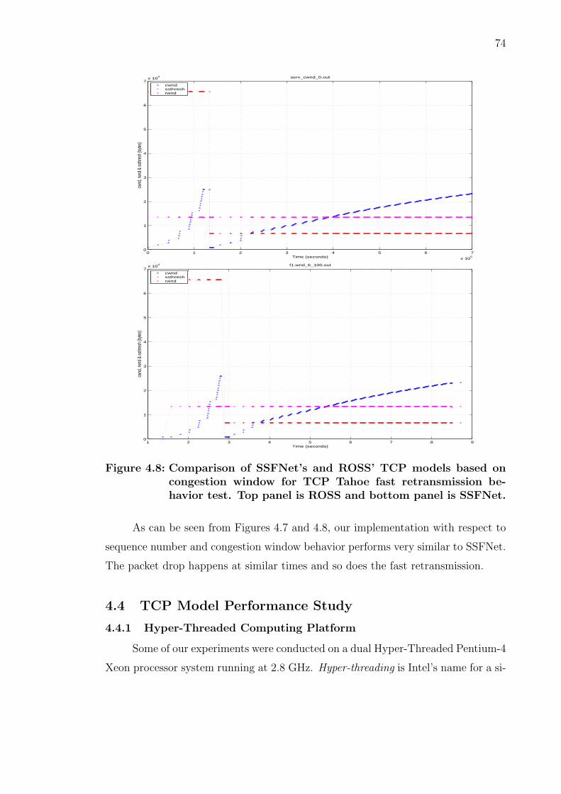
74

0 1 2 3 4 5 6 7

x 105

0

1

2

3

4

5

6

7x 10

4

Time (seconds)

cwnd

, rwn

d & ss

thres

h (by

tes)

serv_cwnd_0.out

cwndssthreshrwnd

1 2 3 4 5 6 7 8 90

1

2

3

4

5

6

7x 10

4

Time (seconds)

cwnd

, rwn

d & ss

thres

h (by

tes)

f1.wnd_6_100.out

cwndssthreshrwnd

Figure 4.8: Comparison of SSFNet’s and ROSS’ TCP models based oncongestion window for TCP Tahoe fast retransmission be-havior test. Top panel is ROSS and bottom panel is SSFNet.

As can be seen from Figures 4.7 and 4.8, our implementation with respect to

sequence number and congestion window behavior performs very similar to SSFNet.

The packet drop happens at similar times and so does the fast retransmission.

4.4 TCP Model Performance Study

4.4.1 Hyper-Threaded Computing Platform

Some of our experiments were conducted on a dual Hyper-Threaded Pentium-4

Xeon processor system running at 2.8 GHz. Hyper-threading is Intel’s name for a si-

75

multaneous multithreaded (SMT) architecture [62]. SMT supports the co-scheduling

of many threads or processes to fill-up unused instruction slots in the pipeline caused

by control or data hazards. Because the system knows that there can be no con-

trol or data hazards between threads, all threads or processes that are ready to

execute can be simultaneously scheduled. In the case of threads that share data,

mutual exclusion is guarded by locks. Consequently, the underlying architecture

need not know about shared variables or how they are used at the program level.

Additionally, because the threads assigned to the same physical processor share the

same cache, there is no additional hardware needed to support a cache-coherency

mechanism.

Intel’s Hyper-Threaded architecture supports two instruction streams per proces-

sor core [47]. From the OS scheduling point-of-view, each physical processor appears

as if there are two distinct processors. Under this mode of operation, an application

must be threaded to take advantage of the additional instruction streams. The dual-

processor configuration behaves as if it was a quad processor system. Because of

multiple instruction streams per processor, we denote instruction stream (IS) count

instead of processor count in our performance study to avoid confusing the issue

between physical processor counts and virtual processors or separate instruction

streams.

The total amount of physical RAM is 6 GB. The operating system is Linux,

version 2.4.18 configured with the 64 GB RAM patch. Here, each process or group

of threads (globally sharing data) is limited to a 32 bit address space, where the

upper 1 GB is reserved for the Linux kernel. Thus, an application is limited to

3 GB for all code and data (both heap and stack space and thread control data

structures).

4.4.2 Quad and Dual Pentium-3 Platform

For the quad processors platform we used the platform mentioned in 3.4.2.

For the dual platform we had a cluster of 40 dual processor machines at .9GHz

connected by 100Mbit Ethernet. Each dual processor machine had 512MB of main

memory and 256 KB of L2 cache.

76

4.4.3 TCP Model’s Configuration

For all experiments for the AT&T and the synthetic topologies, each TCP con-

nection maintains a consistent configuration. The transfer size was infinite, leading

to the transfers running for the duration of the simulation. The maximum segment

size was set to 960 bytes and the total size of all headers was 40 bytes. The packet

size was 1,000 bytes which was consistent with the size used in the SSFnet’s vali-

dation tests. The Initial sequence number was initialized to zero and the slow start

threshold was 65,536.

We did, however, have a window size of 16 for the one million host case which

differed from the default window size of 32. We set the window to 16, hoping to cut

down on the number of packets in the system. Later we found out that changing

the window size did not have an impact due to the limits on the bandwidth in the

system. The congested links force the TCP window to shrink so that the slow-

start threshold became small and the upper bounds on the window size is never

encountered. A similar behavior has been recently noted in [71].

All clients and servers in the AT&T and the synthetic topologies were con-

nected by having the first half of hosts randomly connect to the second half of hosts.

There was a distinct client-server pair for each TCP connection in the simulation.

Because of the random nature of connections, there was a high percentage of “long-

haul” links that resulted in a large number of remote events scheduled between

threads.

4.4.4 Synthetic Topology Experiments

The synthetic topology was fully connected at the top and had 4 levels. A

router at one level had N lower level routers or hosts connected. The number of

nodes was equal to N4 + N3 + N2 + N . N was varied between, 4, 8, 16, and 32.

The nodes were numbered in such a way that the next hop could be calculated on

the fly at each hop.

The bandwidth, delay and buffer size for the synthetic topology is as follows:

• 2.48 Gb/sec, a delay of 30 ms, and 3 MB buffer,

• 620 Mb/sec, a delay between 10 ms to 30 ms, and 750 KB buffer,

77

• 155 Mb/sec, a delay of 5 ms, 10ms and 30ms, and 200 KB buffer,

• 45 Mb/sec, a delay of 5 ms, and 60 KB buffer,

• 1.5 Mb/sec, a delay of 5 ms, and 20 KB buffer,

• 500 Kb per second, a delay of 5 ms, and 15 KB buffer

Here, we considered 3 bandwidth scenarios: (i) high, which has 2.48 Gb/sec

for the top-level router link bandwidths, and each lower level in the network topology

uses the next lower bandwidth shown above yielding a host bandwidth of 45 Mb/sec,

(ii) medium, which starts with 620 Mb/sec and goes down to 1.5 Mb/sec at the

end host, and (iii) low, which starts with 155 Mb/sec and goes down to 500 Kb/sec

at the end host. We note that these bandwidths and link delays are realistic relative

to networks in practice.

Our tests were run on 1, 2 and 4 instructions streams (IS). The synthetic

topology was mapped with each core router and all its children mapped to the same

processor.

Table 4.2 shows the performance results for all synthetic topology scenarios

across varying numbers of available instruction streams on the Hyper-Threaded

system. For all configurations, we report an extremely high degree of efficiency.

The lowest efficiency is 97.4% and to our surprise we observe a large number of

zero rollback cases for 2 and 4 instruction streams resulting in 100% simulator

efficiency. We observe that the amount of available work per instruction stream

retards the rate of forward progress of the simulation, particularly as N grows and

the bandwidth increases. Thus, remote messages arrive ahead of when they need

to be processed resulting in almost perfect simulator efficiency. This result holds

despite an inherently small lookahead which is a consequence of link delay and

relatively large amount of remote schedule work, which ranges from 7% to 15%.

Recall, our link delays range from a small as 5 ms at the low network levels to only

about 30 ms at the top router level.

The observed speedup ranges between 1.2 and 1.6 on the dual-hyper-threaded

processor system. These speedups are very much in line with what one would expect,

particularly given the memory size of the models at hand relative to the small level-2

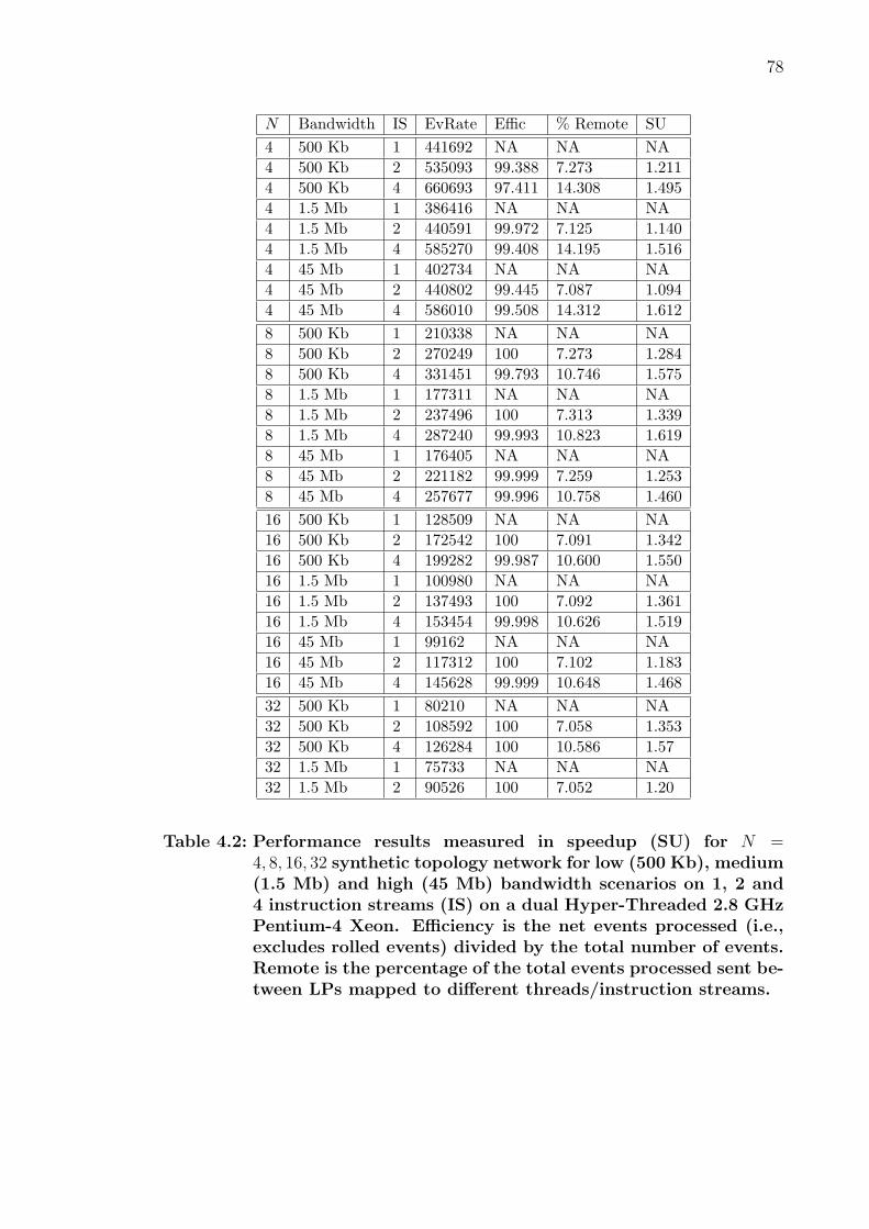
78

N Bandwidth IS EvRate Effic % Remote SU4 500 Kb 1 441692 NA NA NA4 500 Kb 2 535093 99.388 7.273 1.2114 500 Kb 4 660693 97.411 14.308 1.4954 1.5 Mb 1 386416 NA NA NA4 1.5 Mb 2 440591 99.972 7.125 1.1404 1.5 Mb 4 585270 99.408 14.195 1.5164 45 Mb 1 402734 NA NA NA4 45 Mb 2 440802 99.445 7.087 1.0944 45 Mb 4 586010 99.508 14.312 1.6128 500 Kb 1 210338 NA NA NA8 500 Kb 2 270249 100 7.273 1.2848 500 Kb 4 331451 99.793 10.746 1.5758 1.5 Mb 1 177311 NA NA NA8 1.5 Mb 2 237496 100 7.313 1.3398 1.5 Mb 4 287240 99.993 10.823 1.6198 45 Mb 1 176405 NA NA NA8 45 Mb 2 221182 99.999 7.259 1.2538 45 Mb 4 257677 99.996 10.758 1.46016 500 Kb 1 128509 NA NA NA16 500 Kb 2 172542 100 7.091 1.34216 500 Kb 4 199282 99.987 10.600 1.55016 1.5 Mb 1 100980 NA NA NA16 1.5 Mb 2 137493 100 7.092 1.36116 1.5 Mb 4 153454 99.998 10.626 1.51916 45 Mb 1 99162 NA NA NA16 45 Mb 2 117312 100 7.102 1.18316 45 Mb 4 145628 99.999 10.648 1.46832 500 Kb 1 80210 NA NA NA32 500 Kb 2 108592 100 7.058 1.35332 500 Kb 4 126284 100 10.586 1.5732 1.5 Mb 1 75733 NA NA NA32 1.5 Mb 2 90526 100 7.052 1.20

Table 4.2: Performance results measured in speedup (SU) for N =4, 8, 16, 32 synthetic topology network for low (500 Kb), medium(1.5 Mb) and high (45 Mb) bandwidth scenarios on 1, 2 and4 instruction streams (IS) on a dual Hyper-Threaded 2.8 GHzPentium-4 Xeon. Efficiency is the net events processed (i.e.,excludes rolled events) divided by the total number of events.Remote is the percentage of the total events processed sent be-tween LPs mapped to different threads/instruction streams.

79

cache. We note that we were unable to execute the N = 32, 45 Mb bandwidth case.

This aspect and memory overheads are discussed in the paragraphs below.

N Bandwidth Max Ev-list Size Mem Size4 500 Kb 4,792 3 MB4 1.5 Mb 5,376 3 MB4 45 Mb 5,376 3 MB8 500 Kb 45,759 11 MB8 1.5 Mb 85,685 17 MB8 45 Mb 86,016 17 MB16 500 Kb 522,335 102 MB16 1.5 Mb 1,217,929 202 MB16 45 Mb 1,380,021 226 MB32 500 Kb 5,273,847 1,132 MB32 1.5 Mb 6,876,362 1,364 MB

Table 4.3: Memory requirements for N = 4, 8, 16, 32 synthetic topologynetwork for low (500 Kb), medium (1.5 Mb) and high (45 Mb)bandwidth scenarios on 1, 2 and 4 instruction streams on adual Hyper-Threaded 2.8 GHz Pentium-4 Xeon. Optimisticprocessing only required 7,000 more event buffers (140 byteseach) on average which is less 1 MB.

The memory footprint of each model is shown as a function of nodes and

bandwidth in Table 4.3. We report a steady increase in the memory requirements

and the event-list sizes as the bandwidths and the number of nodes in the net-

work increase. The peak memory usage is almost 1.4 GB of RAM for the N = 32,

1.5 Mb bandwidth scenario. The amount of additional memory allocated for opti-

mistic processing is 7,000 event buffers which is less than 1 MB. Thus, for 524,288

TCP connections, this model only consumes 2.6 KB per connection including event

data. By comparison, Nicol [71] reports that NS consumes 93 KB per connection,

SSFNet (Java version) consumes 53 KB, JavaSim consumes 22 KB per connection

and SSFNet (C++ version) consumes 18 KB for the “dumbbell” model which con-

tains only two routers. Our topology is obviously different from the dumbbell model

thereby the memory usages are not directly comparable.

Last, we find that there is an interplay in how the event population is effected

by the network size, topology, bandwidth and buffer space. In examining the mem-

80

ory utilization results, we find that the maximum observed event population differs

by only a moderate amount for the 1.5 Mb versus the 45 Mb case when N = 16

despite a rather significant change in the network buffer capacity. However, we were

unable to execute the 45 Mb scenario when N = 32 because it requires more than

17,000,000 events, which is the maximum we can allocate for that scenario without

exceeding operating system limits. This is because there are many more hosts at

a high bandwidth, resulting in much more of the available buffer capacity to be

occupied with packets waiting for service. This case results in a 2.5 times increase

in the amount of required memory. This suggested, model designers will have to

perform some capacity analysis, since networks memory requirements may explode

after passing some size, bandwidth or buffer capacity threshold, as observed here.

4.4.5 Hyper-Threaded vs. Multiprocessor System

SysConfig EvRate % Effic % Remote SU1 IS, Hyper-Threaded 220098 NA NA NA2 IS, Hyper-Threaded 313167 100 0.05 1.424 IS, Hyper-Threaded 375850 100 0.05 1.711 PE, Pentium-III 101333 NA NA NA2 PE, Pentium-III 183778 100 0.05 1.814 PE, Pentium-III 324434 100 0.05 3.20

Table 4.4: Performance results measured in speedup (SU) for N = 8 syn-thetic topology network medium bandwidth on 1, 2 and 4 in-struction streams (dual Hyper-Threaded 2.8 GHz Pentium-4Xeon) vs. 1, 2 and 4 processors (quad, 500 MHz Pentium-III)

In this series of experiments we compare a standard quad processor system

to our dual, hyper-threaded system in order to better quantify our performance

results relative to past processor technology. The network topology is the same as

previously described with N = 8, thus there are 4,680 LPs in this simulation. We

did however, modify the TCP connections such that they are more locally centered.

So, in total 87% of all TCP connections were within the same kernel process (KP)

which reduced the amount of remote messages.

We observe that the dual processor with hyper-threading out performs the

81

quad processor system without hyper-threading by 16%. The respective speedups

relative to their own sequential performance are 3.2 for the quad processor and 1.7

for the dual hyper-threaded system.

Additionally, we observe 100% simulator efficiency for all parallel runs. We

attribute this phenomenon to the low remote messages and large amount of work

(event population) per unit of simulation time.

4.4.6 AT&T Topology

Figure 4.9: AT&T Network Topology (AS 7118) from the Rocketfuel databank for the continental U.S.

The core US AT&T network topology contains 13,173 router nodes and 38,164

links. What makes Internet topologies like the AT&T network both interesting and

challenging from a modeling prospective is the sparseness and power-law struc-

ture [98] that they exhibit. In the case of AT&T, there are less than 3 links per

router on average. However, at the super core there is a high-degree of connectiv-

ity. Typically, an Internet service provider’s super core will be configured as a fully

connected mesh. Consequently, backbone routers will have up to 67 connections to

other routers, some of which are other backbone or super core routers and other

82

links to region core routers. Once at the region core level, the number of links per

router reduces and thus the connectivity between other region cores is sparse.

In performing a breath-first-search of the AT&T topology, there are eight

distinct levels. At the backbone, there are 414 routers. Each successive level has

the following router count : 4861, 5021, 1117, 118, 58, 6 and 5 nodes. There were

a number of routers not directly reachable from within this network. Those routers

are most likely transit routers going strictly between autonomous systems (AS).

With the transit routers removed, our AT&T network scenario has 11670 routers.

Link weights are derived based on the relative bandwidth of the link in comparison

to other available links. In this configuration, routing is kept static, however, we do

have dynamic routing currently working on a light-weight OSPF model in which we

plan to integrate with our TCP model in the very near future.

The bandwidth, delay, and buffer size for the AT&T topology is as follows:

Level 0 router: 9.92 Gb/sec with a delay randomly selected between 10 ms to 30

ms, and 12.4 MB buffer; Level 1 router: 2.48 Gb/sec, a delay selected randomly

between 10 ms to 30 ms, and 3 MB buffer; Level 2 router: 620 Mb/sec with a delay

selected randomly between 10 ms to 30 ms, and 750 KB buffer; Level 3 router:

155 Mb per second with a delay of 5 ms, and 200 KB buffer; Level 4 router: 45

Mb per second, a delay of 5 ms, and 60 KB buffer; Level 5 router: 1.5 Mb/sec, a

delay of 5 ms, and 20 KB buffer; Level 6 router: 1.5 Mb per second, a delay of 5

ms, and 20 KB buffer; Level 7 router: 500 Kb per second, a delay of 5 ms, and 5

KB buffer; link to all hosts: 70 Kb per second, a delay of 5 ms, and 5 KB buffer.

Hosts are connected in the network at PoP level routers. These routers only

have one link to another higher-level router. In the medium size configuration there

where 10 hosts per PoP level router which totaled 96,500 nodes (hosts plus routers).

In the large configuration there where 30 hosts per PoP totaling 266,160 LPs. In each

configuration, half the hosts establish a TCP session to a randomly selected receiving

host. We observe this configuration is almost pathological for a parallel network

simulation because the amount of remote network traffic will be much greater than

is typical in practice. The amount of remote message traffic is much greater than the

synthetic network topology because of the networks sparse structure. Our goal is to

83

SysConfig EvRate % Effic % Remote SUmedium, 1 IS 138546 NA NA NAmedium, 2 IS 154989 99.947 52.030 1.12medium, 4 IS 174400 99.005 78.205 1.25large, 1 IS 127772 NA NA NAlarge, 2 IS 143417 99.956 51.976 1.12large, 4 IS 165197 99.697 78.008 1.29

Table 4.5: Performance results measured in speedup (SU) for AT&T net-work topology for medium (96,500 LPs) and large (266,160LPs) on 1, 2 and 4 instruction streams (IS) on the dual-hyper-threaded system.

demonstrate simulator efficiency under high-stress workloads for realistic topologies.

We observe over 99% efficiency for the 2 and 4 IS runs as shown in Table 4.5,

yet there is a substantial reduction in the overall obtain speedup. Here, we report

speedups for the 4 IS cases of 1.25 for the medium size network and 1.29 for the

large. We attribute this reduction to enormous amounts of remote messages sent

between instruction streams/processors. The AT&T network topology for a round-

robin mapping results in 50% to almost 80% of all processed events being remotely

scheduled. We hypothesize that the behavior on the part of the model reduces the

memory locality and results in much higher cache miss rates. Consequently, all

instruction streams are spending more time stalled waiting for memory requests to

be satisfied. However, we note that more investigation is required to fully understand

this behavior.

The memory requirements for the AT&T scenario were 269 MB for the medium

size network and 328 MB for the large size network. This yields a per TCP connec-

tion overhead of 2.8 KB and 1.3 KB respectively. The reason for the reduction per

connection is that the amount of network buffer space, which effects the peak event

population, did not change but the number of connections increased.

4.4.7 Campus Network

The campus network has been used to benchmark many network simula-

tors [35, 61, 92, 93, 101] and is an interesting topology for network experimen-

tation [29]. The campus network is shown in Figure 4.10 and is comprised of 4

84

Figure 4.10: Campus Network [59].

servers, 30 routers, and 504 clients for a total of 538 nodes [59]. Limitations in our

TCP model caused us to have 504 servers but our model is still comparable. We

will therefore refer to our campus network model as having 538 nodes for ease of

comparison.

The campus network is comprised of 4 different networks. Network 0 consists

of 3 routers, where node zero is the gateway router for the campus network. Network

1 is composed of 2 routers and the servers. Network 2 is comprised of 7 routers, 7

LAN routers, and 294 clients. Network 3 contains 4 routers, 5 LAN routers, and 210

clients [35]. All routers links have a bandwidth of 2Gb/s and have a propagation

delay of 5ms with the exception of the network 0 to network 1 links, which have a

delay of 1ms. The clients are connected to their LAN routers with links of bandwidth

85

Figure 4.11: Ring of 10 Campus Networks [35].

100Mb/s and 1ms delay.

For our experiments we connected multiple campus networks together at their

gateway routers to form a ring. The links connecting the campus together were

2Gb/s with delays of 200ms. Figure 4.11 shows a ring of 10 of these campuses

connected. The traffic was comprised of clients in one domain connecting to the

server in the next domain in the ring. The server would transfer 500,000 bytes back

to the client application.

We connected 1,008 campus networks together to create a network of the size

542,304. Graph 4.12 shows a super linear speedup on the one processor case per

node but not on the two processor case. This can be attributed to the decrease in

context switching from the two processor per node case. This is a similar result to

86

0

1e+06

2e+06

3e+06

4e+06

5e+06

6e+06

7e+06

8e+06

9e+06

1e+07

4 8 16 18 24 28 36 48 56 72

Pac

ket R

ate

Number of Processors

Distributed ROSS: TCP-Tahoe Model

1 CPU per Node2 CPU per Node

Linear Performance

Figure 4.12: Packet rate as a function of the number of processors.

what was observed in the Network Atomic Operations paper [8]. Our fastest packet

rate of 8.7 million packets per second was observed on 72 processors.

2 nodes 4 nodes 8 nodes 16 nodes 32 nodesROSS 341853 p/s 730720 p/s 1493702 p/s 2817954 p/s 5508404 p/sNS X X X in swap 1069905 p/s

Table 4.6: Performance results measured for ROSS and PDNS for a ringof 256 campus networks. Only one processor was used on eachcomputing node

We tried to run a model of similar size in PDNS on our cluster but the memory

requirements were too high. The largest PDNS model that we could get to run was

137,728 and this was on 32 nodes. We were able to execute this model on two

87

nodes in ROSS and the results and performance numbers can be seen in Table 4.6.

ROSS was able to achieve 5.5 million packets per second whereas PDNS processed

1.07 million packets per second. This shows that our ROSS implementation has

a significantly smaller memory footprint and can achieve 5.14 times speedup over

PDNS.

4.5 Related Work

For networking models much of the current research in parallel simulation

is largely based on conservative algorithms. For example, PDNS [94] is a paral-

lel/distributed network simulator that leverages HLA-like technology to create a

federation of NS [74] simulators. SSFNet [26, 99] and TasKit [110] use Critical

Channel Traversing (CCT) [110] as the primary synchronization mechanism. Dart-

mouth implementation of SSF (DaSSF) employs a hybrid technique called Composite

Synchronization [72].

Recent optimistic simulation systems for network models include TeD [82],

which is a process-oriented framework for constructing high-fidelity telecommuni-

cation system models. Premore and Nicol [85] implemented a TCP model in TeD,

however, no performance results are given. USSF [87] is an optimistic simulation sys-

tem that dramatically reduces model runtime state by LP aggregation, and swapping

LPs out of core. Additionally, USSF proposes to execute simulation unsynchronized

using their NOTIME approach. Based on the results here, a NOTIME synchroniza-

tion could prove beneficial for large-scale TCP models. Unger et. al. simulate a

large-scale ATM network using an optimistic approach [104]. They report speedups

ranging from 2 to 7 on 16 processors and indicate that optimistic outperforms a

conservative protocol on 5 of the 7 tested ATM network scenarios.

Finally, Genesis (The General Network Simulation Integration System), is a

novel approach to scalably and efficiently simulate networks. The Genesis system

divides the networks into domains and simulates each with a separate processor

for a given time interval. Packet-level simulation is done for each domain but syn-

chronizations of the flows are done over the time interval. Upon finishing each

simulation, the domains exchange information about the flows and starts a new it-

88

eration over the same time interval. This continues until all simulations converge,

and then the system moves to a new time interval. This method has been proven

successful in many difficult tasks, such as accurately simulating TCP (Transmission

Control Protocol), which constantly adjusts to network conditions [90, 102].

4.6 Conclusions

The parallel TCP model proved to be extremely efficient with very few roll-

backs observed. Parallel simulator efficiency ranged between 97 to 100% (i.e., zero

rollbacks). The model was implemented to be as memory efficient as possible which

allowed for the million node topology to be executed. We observed model mem-

ory requirements between 1.3 KB to 2.8 KB per TCP connection depending on

the network configuration (size, topology, bandwidth and buffer capacity). Our ex-

periments on the campus network showed excellent performance and super-linear

speedup. We also showed our simulator was 5.14 times faster then PDNS and that

its memory footprint was significantly smaller.

Last, the hyper-threaded system was able to provide a low cost-performance

ratio. What is even more interesting is that these systems blur the lines in terms

of sequential versus parallel processing. Here, to obtain higher rates of performance

from a single processor, one has to resort to executing the model in parallel.

CHAPTER 5

Reverse Memory Subsystem

5.1 Introduction

One of the more difficult problems simulation developers face is designing ef-

ficient models. There are two major domains of efficiency to be concerned with:

memory and computation. The performance of large-scale simulation relies primar-

ily on the memory usage of the system. Traditional state saving solutions have been

shown to be an unacceptable solution, often requiring several times the amount of

sequential memory required. An alternative to state saving is reverse computation.

The tradeoff is that modelers must not only create models of complex problems,

but also their reverse computation as well. One difficulty with constructing an ef-

ficient reversible model is managing memory in both the forward and the reverse

computations. To date, reverse computation lacks a simple mechanism for dynamic

operations over static memory.

While reverse computation has been shown to consistently outperform both

conservative and optimistic (with state saving) methods of simulation, it does not

overcome state saving entirely. Destructive operations must still be state saved in

some form. Floating point operations are typical examples because of the loss of

precision given operations such as divide and multiply. The usual solution is to save

the variable by swapping the destroyed value with a variable in the event. In the

forward execution of an event, the value of the logical process (LP) state variable

is swapped with the event variable. During a rollback, the value of the LP state

variable is restored not by reverse computation, but rather by swapping back the

event variable. Both the state and the event variables are then restored. This is a

form of limited state saving.

Another similar example is memory. LP states are typically more complex

than simple variables; LPs typically contain data structures and user defined objects.

89

90

These objects cannot be reverse computed without a large amount of effort on the

part of the model designer. Further, any solution implemented within the model

would likely take the form of state saving. As a generic example, consider a simple

link list referenced within an LP state. During the execution of an event, an item

in the list must be deleted. Because this event may be rolled back, this list element

cannot simply be freed. Instead, a reference to the element must be saved for

reverse computation. This requires state saving because the list element cannot be

immediately reclaimed.

A reverse memory subsystem is required to address the problem of reverse

computing memory in an efficient way. Our Time Warp system maximizes cache

locality for events, and we apply this same technique in the reverse memory sub-

system. We will show in this thesis that reverse memory is plausible, and enhances

performance greatly. This new subsystem for reverse computing memory completes

the reverse computation solution.

5.2 Design Decisions

Certain assumptions were made in the design of our reverse memory subsys-

tem. The first challenge was how to statically allocate the memory that the model

would use throughout the lifetime of the simulation. For this purpose we chose

to allow the model to configure the amount and size of memory buffers. We con-

strained each memory initialization to be an array of fixed width memory buffers.

This simplifies the reverse memory subsystem greatly because when memory buffers

are needed or reclaimed, they are pulled from a single location. Offering models the

ability to allocate dynamic width memory buffers creates an overly complex memory

subsystem which would introduce fragmentation and would require a replacement

algorithm. Because we want our models to be as efficient as possible, we eliminated

this requirement by constraining the memory buffer sizes to a fixed width. This

is not too tight of a restriction on the model because each pool defines a different

width memory buffer, and the number of pools allocatable is only limited by the

physical memory available. Our intention was not to redesign or build a full memory

management system, but instead to provide the ability to allocate memory on the

91

fly in a simple and efficient manner.

Actual dynamic memory calls within the model can lead to severe performance

penalties and it is a well-accepted best practice to avoid them. Calls to malloc and

free carry a large penalty in a CPU intensive system. The average time to perform

1,000 sequential calls to malloc is ˜7 µs and the cost of the same number of sequential

frees is ˜1-2 µs for a 1KB allocation. One solution is to statically allocate the memory

in the init phase of a simulation, and realize memory operations through this pool

of memory. This pool can be used to fulfill the models’ memory needs, however, the

worst-case memory usage must be assumed. In order to use a statically allocated

memory pool, all of the memory required by the model must be provided in order

for the model to execute.

Models typically use memory in one of two forms: within the LP or model

global state, and within the event buffers themselves. Our CAVES model primarily

uses memory to creates a linked list of views within the LP state. Another example

is a simple router network model. Routers send update messages; these updates can

be variable in size. We could have the message be the size of the maximum update,

but that is an inefficient solution because it assumes a worst-case allocation. We

could have messages of variable sizes. Certain message sizes are not going to be

used as frequently and the modeler would have to estimate the number of messages

needed for each size to perform the static allocation. In addition, there is the

hidden cost of copying the message date to the receiver’s state. Instead, if we store

the updates in a memory buffer, and attach the updates to the events, the receivers

can simply unlink the updates from the event. This eliminates the copy, and allows

for a greater amount of memory reuse. For these types of memory usages it is clear

that a memory subsystem could be helpful. These building blocks can be linked

together and attached to events, and then used in the state of the LPs through a

pointer-based implementation. The pointers can be used in the state in all manners

of data structures, including: lists, trees, hashes and queues.

These building blocks seem to easily fulfill the needs of simple models. The

more difficult needs can still be met. For example, with an Internet routing protocol

model, the routers send dynamic list data structure so that an arbitrary number of

92

hops can appear in the routes. These routes are comprised of lists of integers. If

the building block’s data size was defined as an integer, the overhead of the block’s

other components, would make up the majority of the size. A better but more

difficult way to use the building blocks would be to have the building block’s data

component be the average or median size of the routes. This way the overhead of

the building block’s other components are not the dominating factor. There will

be internal fragmentation of the memory in the building blocks for the routes with

small hop counts or the ones with hop counts larger then the average. This is still

better than having the messages be allocated with the worst case route size.

5.3 Reverse Computing Memory

In the forward execution of an event, if an LP state variable is incremented,

then during a rollback of the same event, the LP state variable should be decre-

mented. This is the definition of reverse computation. When this technique is

applied to memory, the questions which arise are: how do we reverse compute a

memory allocation? Or worse, how do we reverse a memory de-allocation? What

does it mean to undo a free operation?

To further complicate matters, memory may be used in one of two ways.

Memory may be allocated, attached to an event, and the event sent to another

LP. Second, memory may be allocated and maintained within the model state for

accounting purposes. Of course some mix of the two is also possible. The location

and use of the memory buffer within the system determines how it should be handled

during event rollback.

In the following sections we will examine the functions and variables required

for the reverse memory subsystem.

5.3.1 Internals of the Reverse Memory Subsystem

In the design decisions we discussed why we chose a memory buffer building

block. For the rest of the chapter the memory buffer building block will be referred

to as a memory buffer. In this subsection we will discuss the implementation of the

reverse memory subsystem.

93

struct tw_memoryq{

int size;int start_size;// the data size to be allocated for each memory bufferint data_size;int grow;

// head and tail of the memory queuetw_memory *head;tw_memory *tail;

};

struct tw_memory{

// next and prev pointers so the memory buffer can be easily// linked into a listtw_memory *next;tw_memory *prev;

// time at which this event can be collectedtw_stime ts;

// data segment of the memory buffer: application definedvoid *data;

};

struct tw_event{

// added memory buffer pointertw_memory *memory;

};

struct tw_kp{

// added processed memory queuestw_memoryq *queues;

};

struct tw_pe{

// added free memory queuestw_memoryq *free_memq;

};

Figure 5.1: New data structures added to ROSS for the Reverse MemorySubsystem.

94

tw_kp_fossil_memory(){

// Nothing to freeif (queue is NULL)

return;

// There are no memory buffers to freeif (All memory buffers are greater than GVT)

return ;

// All memory buffers can be freed to the PEif (All memory buffers are less than GVT,){

Insert all memory buffers into the PE free queue

return ;}

Find memory buffers that can be freed.

Insert memory buffers into the PE free queue

return ;}

Figure 5.2: Kernel Process Memory Buffers Fossil Collection Function.

The reverse memory subsystem is a list of free memory buffers. The memory

buffer (tw memory) and memory list/queue (tw memoryq) data structures are shown

in Figure 5.1. The memory buffer contains a next and prev pointer for list opera-

tions. The memory buffer also has a data pointer for the user defined data and a

time stamp (ts) for fossil collection.

The user defines how many different sizes of memory buffers they wish to

have, along with how many memory buffers of each size are required. The memory

queue data structure (tw memoryq) has a data size variable which is the data size

of memory buffers that are in the queue. The number of initial memory in the queue

is specified with the start size variable. The user also sets the grow factor grow

which indicates how many memory buffers should be allocated if a shortage occurs.

All the memory buffers are linked onto free lists of the correct type. The user can

easily allocate from each list. The free lists are attached to the processing element

(PE) just like the events are attached in ROSS. The variable for the lists is free memq

95

void tw_event_free(){

// Code for freeing the event...// New code for the memory buffer

// remove all memory buffers from the freed eventm = event->memory;while(m){

event->memory = m->next;free m to the correct PE’s free queuem = event->memory;

}}

Figure 5.3: Freeing of an event after annihilation.

and can be seen in Figure 5.1. The processed memory buffers queues are attached to

the Kernel Process (KP). This is again similar to how the ROSS [12, 13] deals with

the processed event lists. KPs were added in ROSS to aggregate the processed event

lists of a collection of LPs. They dramatically reduce fossil collection overheads thus

this justifies our placement of the processed memory buffer lists. More details on

the ROSS’ data structures can be found in Section 3.1.

The placement of the processed memory buffer list guarantees that the or-

der of the list is fully reversible. The memory buffer fossil collection function

(tw kp fossil memory) is called immediately after the event fossil collection func-

tion. The functions follow the same logic just different data types and the memory

fossil collection function can be seen in Figure 5.2. This function checks if memory

buffers can be freed and frees them to the correct PE’s free memory queue.

Functionality was added to the simulation system to correctly free the memory

buffers upon event cancellation due to rollbacks. As stated in Chapter 2, the time

warp system allows for optimistic execution which can lead to rolling back of events.

One step in undoing an event is cancelling the events which it created. The events

that are created are stored on an output queue and anti-messages are sent for those

events upon rollback. If the event has not been processed the anti-message will

annihilate that event. However, if the event has been processed by the destination

96

g_tw_memory_nqueue; Set the number of different memory buffer

// Allocation the number of elements of// size size_of_data with a grow factor

types tw_memory_init( int number_elements, int size_of_data,int grow_factor){

tw_memoryq *free_q;

for all PEs {free_q = get PE’s queue;// initialize the queuefree_q->start_size = number_elements;free_q->data_size = size_of_data;free_q->grow = grow_factor;

tw_memory_allocate(q);}

}

tw_memory_allocate(tw_memoryq *q){int mem_len, mem_sz;

// calculate the size of a memory buffermem_len = sizeof tw_memory + data_size;

// calculate the size of memory needed for the total number of// memory buffersmem_sz = mem_len * start_size;

allocate mem_sz of memory and link the memory buffers together;

return ;}

Figure 5.4: Initialization Functions and Variables for the Reverse Mem-ory Subsystem.

processor the anti-message will cause that event to be rolled back. This leads to a

difficulty in the passing of memory buffers with events. The event with the memory

buffer attached to it could be in multiple states. There is no way the user could

reverse the passing of the memory buffer due to a lack of mutual exclusion. The only

97

appropriate time to free the memory buffer would be on the freeing of the event after

it is annihilated. Therefore, a memory buffer pointer (memory) was added to the

event shown in Figure 5.1. Upon annihilating an event the simulation system checks

the memory buffer pointer and frees the attached memory buffers to the correct lists.

This takes place in the tw event free function and is shown in Figure 5.3.

5.3.2 Reverse Computing Memory Initialization

In order for the users to access the reverse memory subsystem they need to

be aware of the function calls and the correct way of using them. The list of the

functions and variables for initialization is contained in Figure 5.4.

These function calls must be in the main of the simulation model. The

g tw memory queue should be set before the tw init function call. The function

tw memory init must be called for each of the memory buffer types and should be

called after the tw init but before the call to tw run.

5.3.3 Reverse Computing Memory Allocations

Returning to the linked list example, when an event causes an element to

be allocated and added to the list, the reverse of this operation is to remove the

element from the list and free the memory. However, if the rollback is not too long,

this event will soon be re-executed, and the memory likely re-allocated. Dynamic

memory allocations are too intensive to be used in an optimistic system. Static

memory allocation must be used in order to maintain system performance, but it

may not be possible to ascertain the appropriate amount of memory to allocate.

In addition, statically allocated memory must consider the worst case in order to

ensure model completion.

Our reverse memory subsystem significantly reduces the complexity of simula-

tion models by providing a statically allocated pool of memory for model allocations.

The pool has the ability to grow in the event that it is exhausted, a dynamic mem-

ory allocation which can be amortized across all allocations such that it has no sum

affect on the model. The call for allocating a memory buffer is in Figure 5.5.

The tw memory alloc function returns a tw memory pointer that is simply a

pointer to a memory location, safe to use by the model. The memory buffer pool

98

tw_memory * tw_memory_alloc(tw_lp * lp, tw_fd fd)

{

queue = get PE’s queue ;

if(queue is empty)

tw_memory_allocate(q);

return (remove/pop memory buffer from queue);

}

Figure 5.5: The allocation function for the Reverse Memory Subsystem.

is attached to the LPs tw lp processing element (PE) within ROSS. The tw fd file

descriptor is an index to the correct memory pool to use. Memory pools may be

defined to have different size memory buffers.

During the reverse computation of the event, the call shown in Figure 5.6 is

made to reverse compute the memory allocation. The function expects a pointer to

the memory buffer m that will be reverse allocated, along with the file descriptor fd

for the correct memory pool. This function should not be used when the new allo-

cated memory buffer is sent in an event. The simulation system will automatically

free the buffer in that case.

void tw_memory_alloc_rc(tw_lp * lp, tw_memory * m, tw_fd fd)

{

push memory buffer onto the PE’s free queue;

}

Figure 5.6: The reverse allocation function for the Reverse Memory Sub-system.

Upon reversing the allocation, the memory buffer is simply returned to the

proper pool.

99

5.3.4 Reverse Computing Memory De-allocations

The reverse computing a memory de-allocation is more difficult because an

event which causes a de-allocation may later be rolled back. During a rollback, the

memory buffer which was de-allocated in the forward execution must be restored.

This requires that de-allocated memory be maintained somewhere within the system.

For this purpose a second pool of memory buffers is maintained on the LPs KP.

Within the tw memory free function call the freed memory buffer is inserted into

this queue and the time stamp for the buffer is set. During a rollback, each call

to un-free memory buffers removes the next element in this second pool. Because

causality is enforced at the level of the KP, it is ensured that the memory buffers

will match with the events being rolled back.

The call for freeing memory buffers, and the matching reverse computation

call are shown in Figure 5.7.

void tw_memory_free(tw_lp * lp, tw_memory * m, tw_fd fd)

{

queue = KPs processed memory buffer queue

set time stamp for the m

// Now we need to link this memory buffer into the KP’s

// processed memory queue.

push memory buffer on to the KP’s queue

}

tw_memory *tw_memory_free_rc(tw_lp * lp, tw_fd fd)

{

return (remove/pop memory buffer from the KP’s queue);

}

Figure 5.7: The free and reverse free functions for the Reverse MemorySubsystem.

100

5.3.5 Attaching Memory Buffers to Events

Memory buffers may be allocated and attached to events, which are then sent

to other LPs. This memory buffer must now be considered in the context of the

event, rather than the simple context of the LP. Depending on the state of the

event, the memory buffer must be handled in a special way. Memory buffers can be

attached to events using the routine shown in Figure 5.8. The function expects a

pointer to the event e.

void tw_event_memory_set(tw_event * e, tw_memory * m, tw_fd fd){

if(e has been ABORTED)

{

// frees the memory buffer to the correct PE

tw_memory_alloc_rc( m );

return;

}

attach a memory buffer to the event

return;

}

Figure 5.8: The event memory set function for the Reverse Memory Sub-system.

When this call is made, the memory buffer is placed into a linked list on

the event. However, if the currently allocated event is the abort event (an event

which occurs when event memory has been exhausted), the memory buffer is simply

reclaimed as this event will never be sent or further processed. No reverse function

call is needed to unset a memory buffer. As shown in Figure 5.3 the simulation

system will automatically return the memory buffer to the appropriate pool as the

event is freed.

The call for retrieving memory buffers from a newly received event is shown

in Figure 5.9.

This call returns the memory buffers linked onto the event in reverse order.

But we must also provide a reverse computation call to reverse this process in the

101

tw_memory * tw_event_memory_get(tw_lp * lp)

{

tw_memory *m;

m = event->memory;

if (m)

event->memory = event->memory->next;

return m;

}

Figure 5.9: The event memory get function for the Reverse Memory Sub-system.

event of a rollback because the taking memory buffers off of an event is a destructive

procedure which must be restored. To facilitate this, the call shown in Figure 5.10

is provided.

void tw_event_memory_get_rc(tw_lp * lp, tw_memory * m, tw_fd fd)

{

m->next = event->memory;

event->memory = m;

}

Figure 5.10: The reverse event memory get function for the ReverseMemory Subsystem.

During the forward execution, memory buffers are removed from an event

where the buffers can either be used in the state of the LP or freed using tw memory free.

The reverse computation procedure is to replace the memory buffers on the event.

5.4 Memory Buffers for State Saving

Memory buffers may be allocated for state saving. This can be accomplished

with the above function calls and it will be discussed below.

102

Often the events have extra data in them for state saving. This memory is

often not used all the time which leads to an over allocation of memory in the

system. One example is our TCP model which has 20 bytes for state saving in each

event. Most of the time only 4 bytes are needed. With the use of memory buffers

this over allocation of memory can be reclaimed.

First, the model should no longer use the events for state saving. The TCP

model can use memory buffers. When an event needs to have a memory for state

saving a call to tw memory alloc is executed. The memory buffer is filled in with

the appropriate values and then the model calls the tw memory free on the mem-

ory buffer. This puts the memory buffer on the processed memory list and will be

reclaimed in the fossil collection routine. However, if a rollback occurs the reverse

computation would call tw memory free rc which would return the values of the

destroyed variables. The model can restore these values and then reverse the allo-

cation of the memory buffer with a call to tw rc memory alloc. The benefit of this

technique will be discussed in the performance study.

5.5 Performance Study

For these experiments we ran our tests on the Hyper-Threaded Pentium-4

architecture discussed in Chapter 4’s performance study 4.4.1 and the Pentium-III

architecture discussed in Chapter 3’s 3.4.2.

5.5.1 Benchmark Model

We designed the benchmark model to test all functionalities of the reverse

memory subsystem. The benchmark model mimics phold in its message passing.

Each LP starts off with a linked list of 20 memory buffers and its size is limited to

50 memory buffers. The lists are incorporated into the model to demonstrate how

the reverse memory subsystem can be used in an LP’s state. The LP’s initialization

routine sends messages with up to 3 memory buffers to other LPs. This illustrates

the subsystems capability of passing memory. Upon receiving the message the mem-

ory buffers are added to the LP’s list. This is followed by the LP adding up to 3 or

removing up to 5 memory buffers from its internal list. The LP then creates a new

103

message with up to 3 memory buffers attached to it.

We have created three benchmark models for comparison. The one variant in

each model is how memory is managed. The state saving model makes explicit calls

to malloc and free, the Pre-Allocated model allocates all the memory required for

the model during the initialization phase and uses memory statically, and finally the

reverse computation model which implements the reverse memory subsystem for all

memory management. Each model is identical except for the way in which memory

is managed.

• State Saving: This model variant allows the operating system memory li-

brary to manage memory dynamically throughout the simulation. This model

explicitly calls malloc and free, relying on traditional state saving to support

rollback. This approach would not be chosen in practice because of the high

cost of calling malloc and free. It will also illustrate the memory overheads

of poorly designed state saving models. We created a simple test to measure

the average time to perform 1,000 sequential calls to malloc. The measured

average was ˜7 µs for memory allocations and the cost of the same number of

sequential frees is ˜1-2 µs for a 1KB allocation. For this model there needs to

be 3 memory buffers in every event. There also must be 5 memory buffers in

every event for removed memory.

• Swaps and Pre-allocated Lists: The next approach is to design a model

which allocates a pool of static memory to be used throughout the simulation.

This allocation occurs during the initialization phase of the simulation and so

saves on the cost of calling malloc and free during model execution. However,

this approach requires a worst-case memory allocation in order to support

all possible cases which may arise for a given model. In addition, the model

must implement all of the memory management routines required for memory

allocation/deallocation. The worst case list for this model is initialized with

50 memory buffers. For handling the dynamics in the system there are two

approaches. The first is when a free happens, state save the removed values.

The other approach is, free the memory buffer without state saving the value.

On an allocation, state save the value currently in the freed memory buffer

104

and than use that buffer. For this model let’s perform an analysis. Worst case,

5 memory buffers are removed and no swaps can be performed because the

message values were not installed. In this case 5 memory buffers are required

in the message for state saving. In the allocation case, 6 memory buffers might

be allocated but 3 of the memory buffers can be swapped with the incoming

message values. So the total state saving required is 3 memory buffers. With

this design the free list is used as temporary storage for the removed memory

buffers.

• Reverse Memory Subsystem: The final approach was to use the reverse

memory subsystem. The goal of the subsystem is to statically allocate an

average case amount of memory during the initialization phase, and to provide

highly optimized memory management beyond what is possible within the

model. Because we have access to the internals of the simulator executive,

certain functions can be performed in the reverse memory subsystem which

cannot be handled easily within the model. For example, many operations

within a simulator with speculative execution cannot be committed until after

the GVT time has passed the event time (i.e., I/O operations) because they

cannot be rolled back. The same is true with the reclamation of memory

buffers. The fossil collection routine does not return memory buffers one at

a time to the free memory list. Instead, it “stitches” the subset of memory

buffers from the processed memory queue back into the free memory list. This

detail of memory management is not possible from within the model alone.

Without the reverse memory subsystem, memory buffers attached to events

can only be reclaimed upon event allocation. The reverse memory subsystem

is a highly optimized memory management library with access to all areas

of the simulation executive. The subsystem takes advantage of the fact that

an average case amount of memory may be allocated for the model. If the

simulation causes a worst-case allocation to occur, the simulation executive

may be forced to perform a GVT computation in order to reclaim event and

memory buffers.

105

LPs B Sz St-Sv Swap RMS St-Sv e/s Swap e/s RMS e/s1024 16 5.4 MB 5.1 MB 5.0 MB 306595.31 341213.80 304561.171024 64 14.0 MB 12.1 MB 8.9 MB 201933.67 284425.78 289531.831024 256 47.6 MB 40.0 MB 24.7 MB 138472.08 202924.73 240812.961024 1024 189.4 MB 151.4 MB 87.7 MB 74840.24 102144.14 175813.1816384 16 78.4 MB 73.4 MB 70.7 MB 173536.32 192662.80 178621.8716384 64 204.5 MB 184.4 MB 133.7 MB 136529.00 155620.24 169462.5016384 256 716.4 MB 628.6 MB 385.7 MB 104683.99 121728.00 154630.8116384 1024 2764.3 MB 2405.0 MB 1393.7 MB 67558.10 79469.52 128234.5865536 16 307.9 MB 291.9 MB 280.9 MB 144821.02 156086.62 147415.1765536 64 815.3 MB 735.9 MB 532.9 MB 117703.90 133909.80 143798.67

Table 5.1: Reverse Memory Subsystem memory usage and event rate.LPs the number of LPs in the model. BSz the size of thememory buffers. St − Sv, the state saving model. Swap theswap with statically allocated list model. RMS the ReverseMemory Subsystem

5.5.2 Benchmark Model Results

We ran the experiments on three different sized models and four different sized

memory buffers. The models where comprised of 1024, 16384, and 65536 LPs and

the memory buffers contain either 16, 64, 256, or 1024 bytes. Table 5.1 shows the

memory usage and event rate for the different models. It can be observed that the

model using the reverse memory subsystem had a much smaller memory footprint.

The model using state saving with calls to malloc and free performed the worst.

The reverse memory subsystem, at best, showed a memory savings of 2.17 over the

state saving model. In addition it had a speedup over the state saving model of 2.35

in the 1024 LP and 1024 memory buffer sized case. The interesting result was that

in the smaller memory buffer sized cases, the model with the statically allocated list

performed better than the reverse memory subsystem model. We attribute this to

the fact that the statically allocated list has a better cache performance which is

demonstrated in Table 5.2.

As the memory buffer size increased the performance suffered. This can be

explained by the fact the models had to deal with more data which led to more

cache misses. This can be seen in Table 5.2 which is the profiling results of the

models. It shows the data cache misses for the Pentium 4. This was obtained by

having Oprofile [76] monitor the BSQ CACHE REFERENCE counter with a mask

106

N LPs Buf Sz St-Sv misses Swap misses RMS misses

1024 16 39896 34124 393591024 64 45108 35799 396801024 256 44612 37772 417571024 1024 53906 44706 4449516384 16 42761 35695 4108216384 64 42724 36777 4227916384 256 47574 39488 4336416384 1024 52583 43856 4489165536 16 34953 30854 3525165536 64 35750 32382 36218

Table 5.2: Reverse Memory Subsystem data cache misses. NumLPs thenumber of LPs in the model. BufSz the size of the memorybuffers. St − Svmisses, the state saving model cache misses.Swap the swap with statically allocated list model cache misses.RMS the Reverse Memory Subsystem cache misses.

N LPs Buf Sz 2 Spdup 3 Spdup 4 Spdup

1024 16 1.75 2.39 3.051024 64 1.73 2.36 2.751024 256 1.59 2.00 2.0416384 16 1.63 1.88 1.9916384 64 1.59 2.01 2.0516384 256 1.53 1.84 1.82

Table 5.3: Reverse Memory Subsystem speedup. NumLPs the numberof LPs in the model. BufSz the size of the memory buffers.2− 4Spdup is speedup for 2 to 4 processors.

of 0x100 [24].

The speedup obtained from parallelism is shown in Table 5.3. These results

were performed the quad pentium III’s and our max speedup due to parallelism was

3.05. As model size increased the speedup from parallelism was decreased.

5.5.3 TCP Results

For the performance study we used the synthetic topology which is fully con-

nected at the top and had 4 levels. A router at one level had N lower level routers

or hosts connected. The number of nodes was equal to N4 + N3 + N2 + N . N was

107

N Bandwidth Mem Size Mem Size with buffers4 500 Kb 2.7 MB 2.5 MB4 1.5 Mb 2.8 MB 2.6 MB4 45 Mb 3.5 MB 3.36 MB8 500 Kb 10.8 MB 9.4 MB8 1.5 Mb 17.3 MB 14.9 MB8 45 Mb 17.9 MB 16.3 MB16 500 Kb 101.6 MB 87.8 MB16 1.5 Mb 198.6 MB 165.1 MB16 45 Mb 216.2 MB 179.1 MB32 500 Kb 1,114.3 MB 980.8 MB32 1.5 Mb 1,310.3 MB 1114.3 MB

Table 5.4: Memory requirements for N = 4, 8, 16, 32 synthetic topologynetwork for low (500 Kb), medium (1.5 Mb) and high (45 Mb)bandwidth scenarios on 1, 2 and 4 instruction streams on adual Hyper-Threaded 2.8 GHz Pentium-4 Xeon.

1. DEF(struct, cache) {

2. cache_blk *c_list_h;

3. cache_blk *c_free_h;

4.

5. int free;

6. int used;

7. };

Figure 5.11: CAVES cache data structure.

varied between, 4, 8, 16, and 32. The nodes were numbered in such a way that the

next hop can be calculated on the fly at each hop.

As mentioned above the TCP model had an extra 20 bytes for state saving in

each event. In this test, we removed the state saving from the event and used the

reverse memory subsystem. The result can be viewed in Table 5.4. The performance

between the different models stayed approximately the same while the memory usage

decreased. On average there was a 11.7 percent memory reduction and a best case

reduction of 17.16 percent.

108

Original CAVES:

1. b = cache->c_list_h;

2. temp = b;

3. b = b->next;

4. if(b)

5. b->prev = NULL;

6.

7. if(cache->c_free_h)

8. cache->c_free_h->prev = temp;

9.

10. temp->next = cache_ram->c_free_h;

11. cache->c_free_h = temp;

12. cache->c_list_h = b;

CAVES with the Reverse Memory Subsystem:

1. temp = queue_pop(cache);

2.

3. tw_memory_free(lp,temp, 0);

Figure 5.12: CAVES removal of a view.

5.5.4 Reduction in CAVES Model Complexity

As mentioned before developers often overlook certain optimizations. CAVES

is one such example it has a one to many delete and each LP having a free list. If

the reverse memory subsystem would have been existed, CAVES would have been

implemented with it and the free list would have been move to the KPs. Time

would have not been spent trying to deal with ways of minimizing memory. The

subsystem would have made the design much faster.

In order to support the comparisons being made in this thesis, the CAVES

model was changed to support the reverse memory subsystem. These changes are

discussed below.

With the reverse memory subsystem we also developed a memory queue data

structure which is used in the system for managing the memory buffers. This queue

data structure can be used in models as well and was used in the porting of CAVES

to the reverse memory subsystem.

109

Original CAVES:

1. loc = SV->cache ->c_free_h;

2. SV->cache->c_free_h = loc->next;

3.

4. if ( SV->cache->c_free_h )

5. SV->cache ->c_free_h->prev = NULL;

6.

7. // updates the cache

8. loc->next = SV->cache ->c_list_h;

9. loc->prev = NULL;

10.

11. if(SV->cache ->c_list_h)

12. SV->cache ->c_list_h->prev = loc;

13. SV->cache ->c_list_h = loc;

CAVES with the Reverse Memory Subsystem:

1. loc = tw_memory_free_rc(lp,0);

2. queue_push(&SV->cache, loc);

Figure 5.13: CAVES reverse computation code for a removal of a view.

Original CAVES:

1. b = cache->c_free_h;

2. cache->c_free_h = b->next;

3.

4. if ( cache->c_free_h )

5. cache->c_free_h->prev = NULL;

6.

7. copy_view(M->rc_v, b);

8. init_view(b, M->v);

CAVES with the Reverse Memory Subsystem:

1. b = tw_memory_alloc(tw_getlp(lp),0);

2. init_view(b, M->v);

Figure 5.14: CAVES allocation of a view.

110

Original CAVES:

1. copy_view(b, M->rc_v)

2.

3. if(SV->cache->c_free_h)

4. SV->cache->c_free_h->prev = loc;

5.

6. loc->next = SV->cache->c_free_h;

7. SV->cache->c_free_h = loc;

8. loc->prev=NULL;

CAVES with the Reverse Memory Subsystem:

1. tw_memory_alloc_rc(lp,o_loc,0);

Figure 5.15: CAVES reverse computation of a view allocation

The first thing that can be removed is the data structure for the cache lists

which can be seen in Figure 5.11. This can simply be replaced with a memory queue

for the used cache. Previously the CAVES cache blk were linked together to create

the cache. Now the memory buffers are going to form the link list so the cache blk

next and prev pointers can be removed.

When removing a view from the cache the original CAVES model performed

the code shown in Figure 5.12. The model using the reverse memory subsystem

only needs two lines. Figure 5.13 shows the reverse code for both models.

In an allocation of a cache block, the CAVES original model has to state

save parts of the allocated block. The reverse memory subsystem acts as the log

for state saving and is transparent to the modeler. The freed memory will remain

available until it is fossil collected. Figure 5.14 and 5.15 shows the allocations and

the reversals for the two models.

It can be seen that the code is significantly less complex. One thing to note

is that the memory was not reduced significantly as previously thought. The over

allocation of the cache was fairly small compared to the event population. The main

savings was the reduction of state saving in the event. The state saving was now

moved in to the LP in the form of memory buffers. This was a finding that we were

not expecting. The run-time performance of the two models are comparable, which

111

suggest the overheads introduced by this subsystem are not significant.

5.6 Conclusions

As can be seen the reverse memory subsystem provides better results than

the first passes on model design which indicates that the model design process has

been made simpler. Now modelers do not have to focus on creating their own

memory pool. The simulation system will take care of all the overheads and will

provide close to optimal results. For different types of models it shows that there are

ways to get around the issue of having different sized events. This reverse memory

subsystem gives the tools to allow for quick and more complex models to be created

without much difficulty. The memory reductions and speed up gains over a factor

of 2 from the worst case shows models will be able to be created much better,

faster and without nearly as much experience in an optimistic simulation system.

The subsystem can be used in previous models to gain more optimizations that

modelers might have missed or when too difficult to previously implement. This

is shown in the new CAVES section. Overall this subsystem opens the door and

lowers the development cost for modelers to leverage reverse computation in their

optimistic synchronization models.

CHAPTER 6

Sharing Event Data

6.1 Introduction

One of the more challenging issues in model design is keeping the model size

small. A good way to address this problem is to reduce the amount of duplicate

information. As mentioned in [111], Logical Processes (LPs) that share common

data can have a global data structure which will reduce the total state of the model.

From this, the question of “why must this just be limited to the LPs?” arises. Could

a sharing approach be employed in event data as well? Our experimentation shows

that the answer is yes and one good example is a multicast network model [27]

because of the duplicate nature of the events. However, this approach could be used

in several, more generic model scenarios. In fact, at any point in a model where

an event is to be broadcast to two or more LPs, there can be a significant memory

savings attributed to this approach.

In the multicast protocol, data transmission is minimized by sending messages

through a multicast tree before being broadcast to each subscriber. The goal is to

minimize individual transmissions sent separately to each subscriber. This proto-

col model has duplicate information being sent to each subscriber where there are

branches in the multicast tree. In a simulation with shared memory we have the

ability to have a global view of the system. Typically, a multicast model generates

messages that result in multiple, identical messages being sent to each subscriber

LP in the system. Each LP would then read those messages, update its state, and

possibly generate more events in the system.

Rather than identical events being sent to each subscriber with the same data

attached, we keep a pointer to the data in the event header and send each subscriber

LP this pointer. Each LP is required not to overwrite the data, as it is understood

in the model that this event data is being shared globally throughout the system.

112

113

Our second requirement is that only once each subscriber has received the multicast

event, the attached data can be reclaimed.

This optimization is important because it drastically reduces the most memory

exhaustive component of simulation: the event population. This optimization can

be applied to all types of simulation: sequential, parallel and even distributed.

In this chapter, we will discuss the sequential and parallel implementation of this

approach. Additionally, there are two types of parallel synchronizations. With

sequential and conservative synchronization the implementation of this idea is trivial

because attached data can immediately be reclaimed.

Optimistic simulators pose a greater design and implementation challenge be-

cause processed events are maintained for possible future rollback scenarios. These

scenarios are much more difficult to address because events must have been read by

all receivers prior to reclamation. In fact, there are several cases that are outline in

this chapter where this optimization must be managed properly by the optimistic

simulation executive.

We chose the multicast protocol model as our primary example for this ex-

perimental investigation. We follow with possible implementations of the method

assuming different synchronization mechanisms. There will be a detailed discussion

of the implementation of the method in a discrete event simulation which employs

optimistic synchronization. For the performance results a benchmark multicast-like

model will be used in the evaluation.

6.2 Multicast Background

The multicast protocol is a bandwidth-conserving technology that aims to

reduce packets in a network by transmitting a single stream of data to thousands

of receivers on the network. Many applications take advantage of this protocol,

including: video conferencing, corporate communications, distance learning, and

distribution of just about any type of information.

Multicast has been in use on large scale networks since the introduction of

the Mbone [64] in 1992. Today, Microsoft China has one of the largest multicast

networks, and plans to begin providing multicast television to viewers in 2005 [48].

114

Figure 6.1: Multicast graphic from Cisco [21].

The multicast solution will become widely used on the Internet as a solution to

higher bandwidth costs due to ever increasing numbers of Internet subscribers.

The multicast model works by delivering traffic from a single source to mul-

tiple receivers through the multicast tree. Multicast receivers subscribe to a given

source, and the information is then disseminated through the multicast tree back

to the multicast group of receivers. Internet routers replicate packets at branches

in the multicast tree so that all subscribers will receive the same packet data. This

low-cost solution not only reduces the amount of bandwidth required to transmit

a large stream of data to multiple receivers, it also reduces the number of requests

serviced by the source. The multicast protocol is efficient in its design compared to

other protocols which commonly require the source to send individual copies of the

same information to multiple receivers. When the amount of data being transmitted

is large, it quickly becomes difficult for the source to send multiple copies across a

network, as in the case of MPEG video. A large amount of network resources are

consumed providing an individual stream for each receiver. The multicast protocol

115

can also provide a substantial savings when the data transmitted from the source is

small because there may be thousands of receivers to be serviced. Figure 6.1 demon-

strates how data from a single source is delivered to multiple recipients through a

multicast tree.

Our model of the multicast protocol clearly illustrates the performance impact

of our shared event data optimization. It is easy to see that if we are able to move X

bytes into a shared message and there are 1000 multicast subscribers the savings will

be roughly 1000-fold bytes. Conversely, if X is very large, and there are only a few

receivers, the memory savings will also yield a significant performance improvement

as the large event memory segment would only need to be written into memory

once. Furthermore, as these large packets traverse the network the number of copy

operations is zero.

6.3 Implementation

In order to successfully deploy this new idea in a current simulator executive,

two restrictions must be met. Once the shared event data has been identified, it can

be allocated and written only once, and then dereferenced for each subscriber event

created. The first restriction is that each subscriber may not destroy or modify the

shared event data. The second restriction is that the simulation executive may not

prematurely reclaim the shared event data. Only once each subscriber has received

the event can the shared event data be freed.

6.3.1 Sequential & Conservative Simulation

In a sequential simulation this optimization can easily be implemented entirely

within the model. The modeler can keep a pointer to the shared event data. For

each newly created event that will forward the shared data, the pointer to the shared

data is set. Next, there needs to be a way to free the shared data once the event has

been processed by all subscribers. If the final subscriber is known, the shared event

data can be freed once that subscriber has processed the event. Another approach

is to maintain a counter that indicates the number of sends and receives. When the

last subscriber receives the event and does not forward it to any other subscriber,

116

the counter will be zero and the shared data segment is safe to reclaim. Since the

execution is sequential, only one LP will be accessing the counter at a time and

there is no need for mutual exclusion. Finally, the last subscriber to receive the

event will be the correct one to free it.

With conservative simulation systems such as DaSSF [72], this optimization

can also be implemented by the model. Once again the modeler creates a pointer

in the event message for the shared data segment. Each newly created event that is

going to be forwarding the data can point to the same shared data segment. The

freeing of the data can be done the same way as in the sequential case because in

conservative simulation there are no roll backs and all events executed are processed

in the correct causal order. However, the execution is parallel and so would require

mutual exclusion for the counter if that is the method used to determine the second

restriction.

6.3.2 Optimistic Simulation

Within optimistic simulation there are additional issues to address. In par-

ticular, speculative execution complicates the allocation/deallocation process when

rollbacks occur.

We chose to implement this novel idea within ROSS [12, 13, 14]. ROSS han-

dles causal errors through reverse computation. When a rollback occurs, an event’s

reverse computation event handler is called, which has the inverse effects on the

LP’s state compared to the forward execution of the event. ROSS includes a reverse

memory subsystem which allows for the dynamic allocation of statically allocated

memory. This subsystem was designed to overcome the problem of reverse com-

puting memory operations such as malloc and free during event execution. The

reverse memory subsystem greatly reduces the complexity of many models by al-

lowing them to create memory buffers and either maintain them in their LP state

or to send them as part of the event data. When we discuss reclaiming the shared

event data segments, it is these memory buffers to which we are referring.

Our implementation used a counter within the event header to track subscriber

sends. The easiest implementation of this idea is not to try to reclaim the shared

117

if(e has been ABORTED)

{

if( *b )

{

lock(&((*b)->mem_lck));

if((*b)->counter != 0)

{

unlock(&((*b)->mem_lck));

return;

}

free the memory pointed by event e (i.e., e->memory);

unlock(&((*b)->mem_lck));

*b = NULL;

}

return;

}

lock(&((*b)->mem_lck));

(*b)->counter++;

unlock(&((*b)->mem_lck));

e->memory = *b;

return;

Figure 6.2: Memory Set Routine. This routine is performed when settinga memory buffer to an event. B is the memory buffer. E isthe event.

data when it reaches the end points. The reason is the supposed final end point

might not be the final end point due to the fact that other end points might be rolled

back. In an optimistic solution, the event data segments are reclaimed only once

the possibility of a rollback is eliminated by the passing of the global virtual time

(GVT) [51]. Only those events with a time stamp less than the current GVT value

may be reclaimed by the system [33]. Typically, for caching purposes, those events

are made readily available for the next event creation. This improves the cache

hit rates because we know that the newly reclaimed event is in our cache, and so it

should be the next event to be allocated. On the reallocation of the event the shared

event data can be reclaimed. This method requires additional memory because the

118

if(e->memory)

{

lock(&e->memory->mem_lck);

e->memory->counter--;

if(e->memory->counter == 0 )

{

unlock(&e->memory->mem_lck);

free the memory pointed by event e (i.e., e->memory);

}

else

unlock(&e->memory->mem_lck);

e->memory = NULL;

}

Figure 6.3: Memory free routine. This routine is performed on all eventallocations. B is the memory buffer. E is the event.

shared event data is being reclaimed later in the simulation, but still dramatically

less than the amount of memory needed for a non-shared data approach. Within

the shared data there is a counter and a mutual exclusion lock which the simulation

executive manages. This optimization is entirely transparent to the model.

A second issue is that the execution of an event might not create the desired

new event. For example in ROSS, once all event-memory is allocated, a special

event called the abort event is returned as opposed to returning a null pointer. This

enables regular optimistic processing to continue until the scheduler reaches a point

at which it can correctly and safely re-claim memory. This approach is similar to the

approach taken in the Georgia Tech Time Warp (GTW) [34]. In the “event-send”

routine, if it finds an abort event has been scheduled, it continues processing but

does not send that event. Additionally, when the current event execution completes,

it is rolled back and any events which it created are cancelled.

The steps for the memory set routine are illustrated in Figure 6.2. Here, the

newly allocated memory buffer denoted by b, has its access control counter increased

by one provided the owning event, e, is not the abort buffer. If the abort buffer

is encountered, and the counter is zero, then that shared memory segment is freed.

119

Figure 6.4: Additional Memory Required for Increases in Levels.

Otherwise, this routine returns. Next, Figure 6.3 shows how a shared event segment

is freed. In this routine, the memory segment’s access counter must be zero prior to

the actual release of the memory segment. Please note, critical sections are denoted

by the lock and unlock routines. Both increment and decrement operations of

the access counter variables are “locked”. Additionally, any tests for zero are placed

within the lock since one and only one processor should free a shared memory buffer.

We observe that this interface only affects forward event processing. When a

rollback occurs, the reverse event handling code is not effected and no new function

calls or code modifications are required to support shared event segments.

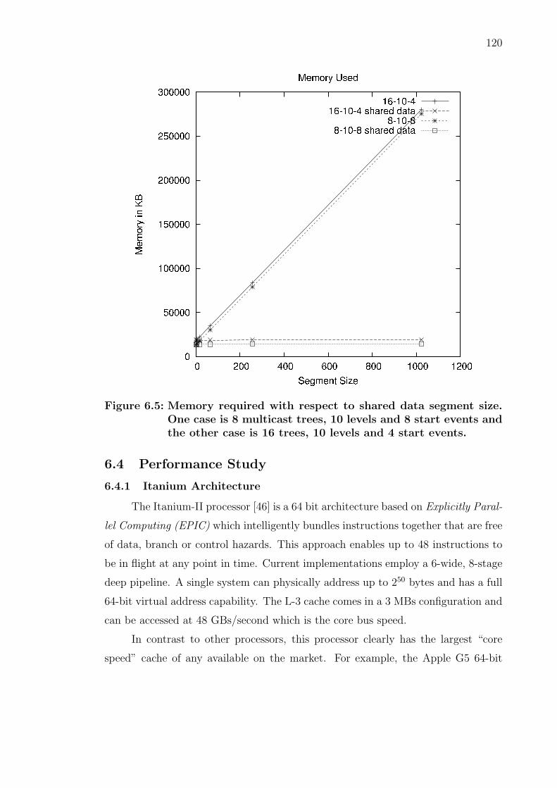
120

Figure 6.5: Memory required with respect to shared data segment size.One case is 8 multicast trees, 10 levels and 8 start events andthe other case is 16 trees, 10 levels and 4 start events.

6.4 Performance Study

6.4.1 Itanium Architecture

The Itanium-II processor [46] is a 64 bit architecture based on Explicitly Paral-

lel Computing (EPIC) which intelligently bundles instructions together that are free

of data, branch or control hazards. This approach enables up to 48 instructions to

be in flight at any point in time. Current implementations employ a 6-wide, 8-stage

deep pipeline. A single system can physically address up to 250 bytes and has a full

64-bit virtual address capability. The L-3 cache comes in a 3 MBs configuration and

can be accessed at 48 GBs/second which is the core bus speed.

In contrast to other processors, this processor clearly has the largest “core

speed” cache of any available on the market. For example, the Apple G5 64-bit

121

Figure 6.6: Event Rate with respect to shared data segment size. Onecase is 8 multicast trees, 10 levels and 8 start events and theother case is 16 trees, 10 levels and 4 start events

processor provides only has 512KB level-2 cache or 14.3% of the available cache

on the Itanium-II processor. However, the core bus speed on this processor is 64

GBs/second.

6.4.2 Benchmark Multicast Model

For the performance study we implemented a benchmark multicast model. We

constructed binary trees to describe the network topology of sources, routers and

subscribers. All of the trees were disjointed. The leaf nodes off the routers were the

subscribers. The source root node was responsible for generating the packets. Once

the packet was received by the left-most subscriber in the tree, the root generates

the next packet.

122

T L Estart S Mtraditional Mshared ERtraditional ERshared

8 10 8 4 14.4 MB 14.8 MB 377986.673 370801.9248 10 8 16 17.4 MB 14.8 MB 350491.922 378053.9708 10 8 64 29.4 MB 14.8 MB 336866.703 377541.4408 10 8 256 77.4 MB 14.9 MB 330823.230 370219.7978 10 8 1024 269.3 MB 15.4 MB 324083.951 367463.72616 10 4 4 19.1 MB 19.4 MB 342921.408 335885.51416 10 4 16 22.1 MB 19.4 MB 322796.458 341562.54316 10 4 64 34.1 MB 19.4 MB 311617.293 342541.11016 10 4 256 82.0 MB 19.6 MB 306166.442 336635.59516 10 4 1024 273.9 MB 20.0 MB 300169.391 333708.05416 15 8 256 4936.3 MB 842.0 MB 137519.194 146734.51016 15 8 1024 17224.1 MB 842.9 MB 57867.255 146681.164

Table 6.1: Sequential Performance with and without shared data. T isthe number of trees in the multicast graph. L denotes thenumber of level within each tree. Estart is the number of initialevents each LP schedules at the start of the simulation. S is thesize of the data size in the messages. Mtraditional and Mshared arethe required memory for the traditional and shared event datamodels respectively. ERtraditional and ERshared are the event ratefor the traditional and shared event data models respectively.

6.4.3 Model Parameters and Results

We experimented with many parameters in the multicast benchmark model.

The most significant model parameters were the number of LPs and the size of the

shared data segments. We varied the number of trees from 2 to 16 and the number

of levels from 5 to 15. A power of two was not chosen because 15 was the largest

number of levels that would still fit into memory. The shared data size ranged from

4 integers to 1024 integers and was modeled using individual memory buffers of the

respective sizes. In addition we varied the number of start events from 2 to 8.

For the first set of experiments we ran ROSS sequentially with and without

a shared data segment in the events. Obviously, as the number of trees and start

events increased the memory increased accordingly. When the number of levels in

the trees grow, an exponential increase in memory usage was experienced. This

can be seen in Figure 6.4 and is explained by the exponential nature of the data

structure.

It can be observed that there was a smaller benefit for the small shared data

123

T L Estart S MRshared MRtraditional % Reduction

8 10 8 4 0.0221 0.0221 0.00 %8 10 8 16 0.0221 0.0211 -4.73 %8 10 8 64 0.0221 0.0231 4.33 %8 10 8 256 0.0224 0.0259 13.51 %8 10 8 1024 0.0224 0.0290 22.75 %16 10 4 4 0.0224 0.0224 0.00 %16 10 4 16 0.0225 0.0213 -5.63 %16 10 4 64 0.0228 0.0234 2.56 %16 10 4 256 0.0228 0.0261 12.64 %16 10 4 1024 0.0229 0.0293 21.84 %

Table 6.2: Data cache misses per memory reference. T is the numberof trees in the multicast graph. L denotes the number oflevel within each tree. Estart is the number of initial eventseach LP schedules at the start of the simulation. MRshared andMRtraditional are the data cache misses rates for the shared eventdata and traditional models respectively. Finally, % Reductionis the amount the miss rate is reduced by the event sharingscheme.

segments. However, in the larger sized data segments the benefits are quite notice-

able. This can be seen in Figures 6.5, 6.6 and Table 6.1. In the larger cases the share

data segments led to significant decreases in memory and increases in performance.

The decrease in memory is explained by the fact that the overhead of the share data

segment is surpassed by the duplicate information. In some cases the shared data

models used 1/20th of the memory required by traditional sequential simulations

(i.e., not sharing event segments). One observed result showed a speedup of 2.5.

This performance is explained by the fact that the traditional model was in swap

and thrashing. For the other data points, the speedup is attributed to a smaller

memory footprint which enables more events to fit in the cache. Another part of

the speedup was the model only had to assign values to pointers instead of copying

data from events.

Table 6.2 is the profiling results of the models. It shows the data cache misses

per memory reference for the shared event data and traditional models. The ratio

was obtained by dividing DCU LINES IN by DATA MEM REFS which are counters

124

T L Estart S 2 PEs 3 PEs 4 PEs

8 10 4 256 1.36 1.95 2.348 10 4 1024 1.35 1.94 2.328 10 8 256 1.49 2.22 2.738 10 8 1024 1.48 2.21 2.748 15 4 256 1.56 2.43 3.218 15 4 1024 1.55 2.43 3.228 15 8 256 1.54 2.41 3.198 15 8 1024 1.54 2.41 3.1916 10 4 256 1.51 2.25 2.8016 10 4 1024 1.51 2.23 2.7916 10 8 256 1.59 2.40 2.9416 10 8 1024 1.59 2.43 2.6416 15 4 256 1.54 2.42 3.2016 15 4 1024 1.53 2.42 3.2016 15 8 256 1.53 2.38 3.0616 15 8 1024 1.54 2.37 3.04

Table 6.3: Parallel results for shared event data. T is the number oftrees in the multicast graph. L denotes the number of levelwithin each tree. Estart is the number of initial events each LPschedules at the start of the simulation. 2-4 PEs is perfor-mance measured in speedup (i.e., sequential execution dividedby parallel execution time) for 2 to 4 processors.

that Oprofile monitored on a Pentium III [23]. The table shows that as the event

data size increases the shared event data model has fewer data cache misses than

the traditional model. These fewer misses can also explain the speedup which is

shown in Table 6.1.

One outlier result was in the 16 integer case, the traditional model had a

better ratio. Certain models are more sensitive than others to how the model fits

into the L2 cache, yielding better performance in some cases. It appears that the 16

integer case was one of these situations. More investigation is needed to determine

the precise effects of caching on performance.

Table 6.3 shows the result of the tests on the 1.5 GHz quad processors Itanium-

IIs. The maximum speedup attain was 3.22 on four processors. The low values of

speedups can be explained by the fact that the system does not have enough work

125

and can be remedied by increasing the number of start events in the system. This

can also be observed in the table.

6.5 Related Work

Much of the research in parallel simulation for shared data was based on

modifying and reading multiple LP’s states. For example sharks world breaks a

model down into sectors and each sector needed to be able to read or modify entities

on its neighbor state [25]. One method would be to use the push method, in which

messages are passed to the correct neighbors with the entities information. The other

way is posed in the space-time memory paper [39]. This concept has shared objects

with a time log attached to them. It allows for an easier model development over

the push method. A distributed method for sharing variables in systems without

physically shared memory was discussed by Mehl and Hammes [66]. The main

difference between our work and these other papers is that our shared memory is

not allowed to be modified. This eliminates the issue of whether the memory is safe

to read.

In the context of shared memory performance optimization, Panesar and Fuji-

moto have two key results. In [77], they present a event buffer management scheme

that reduces memory overheads on a cache-coherent shared memory multiprocessor

(KSR systems). To efficiently avoid over-optimistic execution, as well as ensure that

event memory is equally distributed among all processors, they devised a control

flow technique which treated event memory like a window of network packets and

applied a congestion control approach to throttling Time Warp event processing

rates [78].

Multicast is also used in the High-Level Architecture [33, 45] (also known as

IEEE 1516). This is a general purpose architecture for simulation reuse and interop-

erability. Here, simulators communicate through a publish and subscribe interface.

One of the key challenges is how to correctly disseminate update information. To

address this problem, multicast groups are employed as a means to allow simulators

to subscribe to regions of interest. Each “region” is assigned a multicast group iden-

tifier. This approach enables the efficient dissemination of update information about

126

simulation entities of interest. The key difference here is that our shared-memory

approach reduces memory consumption whereas the HLA’s implementation reduces

network bandwidth, but overall memory consumption remains the same.

Finally, we note that sharing event data has some linkages to multi-resolution

modeling [70]. Here, MRM is primarily concerned with the correct temporal and

spatial aggregation and disaggregation of simulation objects. The key difference

between our approach is that we are only concerned with a spatial aggregation of

event data that would be scheduled to a number of simulation objects at or about the

same point in virtual time. Additionally, we are unaware of any MRM approach for

an optimistic synchronization environment. In particular, how one would rollback

either an aggregation or disaggregation operation is still an open question.

6.6 Conclusions

From the idea of shared data in the LP we transform it into the idea of shared

data in the event. This chapter shows that the idea of shared event data is possible

and shows that there are benefits of 2 to 20 times in memory savings. There are

also speedup gains from this idea due to eliminating the copying for hop to hop. We

report a 22% reduction in the data cache miss rate and in addition we show parallel

speedups of 3.22 on a quad processor system.

CHAPTER 7

Summary

In this thesis we present two large-scale simulation models with reverse computation.

We discussed the benefits from a reverse memory subsystem and shared event data.

The first large-scale model was for a configurable view storage system (CAVES).

This model is suitable for execution on an optimistic simulation engine. Overall, we

find that our model performs well with an average speedup of 3.6 on 4 processors

over all configurations. Many cases yield super-linear speedup, which is attributed

to a slow memory subsystem on the multiprocessor PC. We find that a number

of parameters effect key Time Warp performance metrics. In particular, the view

storage size decreases rollbacks when increased and decreases the total number of

events.

In the second large-scale model, we dispel the view that optimistic simula-

tion techniques operate outside the performance envelop for Internet protocols and

demonstrate that they are able to efficiently simulate large-scale TCP scenarios for

realistic, network topologies using a single hyper-threaded computing system costing

less than $7,000 USD. The model was implemented to be as memory efficient as pos-

sible which allowed for the million node topology to be executed. We observed model

memory requirements between 1.3 KB to 2.8 KB per TCP connection depending on

the network configuration (size, topology, bandwidth and buffer capacity). For our

real-world topology, we use the core AT&T US network. Our optimistic simulator

yields extremely high efficiency and many of our performance runs produce zero roll-

backs. However, the number of remote messages limited the speedup for the AT&T

topologies. Our experiments on the campus network showed excellent performance

and super-linear speedup. We also showed our simulator was 5.14 times faster then

PDNS and that its memory footprint was significantly smaller.

As can be seen the reverse memory subsystem provides better results than the

first passes on model design which indicates that the model design process has been

127

128

made simpler. Now modelers do not have to focus on creating their own memory

pool. The simulation system will take care of all the overheads and will provide close

to optimal results. For different types of models it shows that there are ways to get

around the issue of having different sized events. This reverse memory subsystem

gives the tools to allow for quick and more complex models to be created without

all the difficulties. The memory reductions and speed up gains over a factor of 2

from the worst case shows models will be able to be created much better, faster

and without nearly as much experience in an optimistic simulation system. The

subsystem can be used in previous models to gain more optimizations that modelers

might have missed or when too difficult to previously implement. This is shown in

the new CAVES section. Overall this subsystem opens the door and lowers the

development cost for modelers to leverage reverse computation in their optimistic

synchronization models.

With the addition of this subsystem the modeler will be given the flexibility

to develop more complex models in less time. This subsystem will allow optimistic

parallel simulation to be more common place in the network simulation field.

From the idea of shared data in the LP, we transformed it into the idea of

shared data in the event. Our work shows that the idea of shared event data is

possible and shows that there are benefits of 2 to 20 times in memory savings.

There are also speedup gains from this idea due to eliminating the copying for hop

to hop. We report a 22% reduction in the data cache miss rate and in addition we

show parallel speedups of 3.22 on a quad processor system.

BIBLIOGRAPHY

[1] M. Abrams, C. R. Standridge, G. Abdulla, E. A. Fox and S. Williams.“Removal Policies in Network Caches for World-Wide Web Documents.” InProceedings on Applications, Technologies, Architectures, and Protocols forComputer Communications, 293–305, 1996.

[2] R. Agarwal, C. N. Chuah, S. Bhattacharyya, and C. Diot. “The Impact ofBGP Dynamics on Intra-Domain Traffic.” In Proceedings of SIGMETRICS,2004.

[3] H. Agrawal, R. A. DeMillo, and E. H. Spafford. “An Execution BacktrackingApproach to Program Debugging.” IEEE Software, pages 21-26, 1991.

[4] H. Agrawal, R. A. DeMillo, and E. H. Spafford. “Efficient Debugging withSlicing and Backtracking.” Software Practice & Experience, June 1993, 23(6),pp. 589-616.

[5] M. F. Arlitt, and C. L. Williamson. “Trace-Drive Simulation of DocumentCaching Strategies of Internet Web Servers.” Simulation 68(1): 23-33, 1997.

[6] R. M. Balzer. “EXDAMS: EXtendible Debugging and Monitoring System.” InAFIPS Proceedings, Spring Joint Computer Conference, volume 34, pages567-580, Montvale, New Jersey, 1969. AFIPS Press.

[7] J. Banks, J. S. Carson, II, and B. L. Nelson “Discrete-Event SystemSimulation.”, 2rd Edition. Prentice Hall, Upper Saddle River, New Jersey,1996.

[8] D. Bauer, G. Yaun, C. D. Carothers, M. Yuksel, and S. Kalyanaraman.“Seven-O’Clock: A New Distributed GVT Algorithm Using Network AtomicOperations.” In Proceedings of the Workshop on Parallel and DistributedSimulation (PADS ’05), 2005.

[9] S. Bellenot. “State Skipping Performance with the Time Warp OperatingSystem.” In Proceedings of the Workshop on Parallel and DistributedSimulation (PADS ’92), pages 53-64. January 1992.

[10] D. Bruce. “The treatment of state in optimistic systems.” Proceedings of the9th Workshop of Parallel and Distributed Simulation (PADS’95), 40-49, June1995.

129

130

[11] R. E. Bryant. “Simulation of Packet Communication Architecture ComputerSystems.” Computer Science Laboratory . Massachusetts Institute ofTechnology, 1977.

[12] C. D. Carothers, D. Bauer and S. Pearce. “ROSS: A High-Performance, LowMemory, Modular Time Warp System.” In Proceedings of the 14th Workshopof Parallel on Distributed Simulation (PADS 2000), pages 53-60, May 2000.

[13] C. D. Carothers, D. Bauer, and S. Pearce. “ROSS: A High-Performance, LowMemory, Modular Time Warp System.” Journal of Parallel and DistributedComputing, 2002.

[14] C. D. Carothers, D. Bauer and S. Pearce. “ROSS: Rensselaer’s OptimisticSimulation System User’s Guide.” Technical Report #02-12, Department ofComputer Science, Rensselaer Polytechnic Institute, 2002,http://www.cs.rpi.edu/tr/02-12.pdf

[15] C. D. Carothers, K. S. Perumalla, and R. M.Fujimoto. “Efficient OptimisticParallel Simulations using Reverse Computation.” In Proceedings of the 13th

Workshop on Parallel and Distributed Simulation (PADS’99), 126-135, 1999.

[16] C. D. Carothers, K. S. Perumalla, and R. M. Fujimoto. “Efficient OptimisticParallel Simulations using Reverse Computation.” (journal version). ACMTransactions on Computer Modeling and Simulation (TOMACS), 9(3):224–253, 1999.

[17] C. D. Carothers, K. S. Perumalla, and R. M. Fujimoto. “The Effect ofState-saving in Optimistic Simulation on A Cache-Coherent Non-UniformMemory Access Architecture.” In Proceedings of the 1999 Winter SimulationConference, 1999.

[18] K. M. Chandy and J. Misra. “Distributed Simulation: A Case Study in theDesign and Verification of Distributed Programs.” IEEE Transactions onSoftware Engineering 5 (3): 440-452, 1979.

[19] K. M. Chandy and J. Misra. “Asynchronous distributed simulation via asequence of parallel computations.” Communications of the ACM 24 (4):198-205, April 1981.

[20] D. Chiu and R. Jain. “Analysis of the Increase/Decrease Algorithms forCongestion Avoidance in Computer Networks.” Journal of ComputerNetworks and ISDN, Volume 17, Number 1, pages 1-14, June 1989.

[21] Cisco. “Internet Protocol Multicast.” http:

//www.cisco.com/univercd/cc/td/doc/cisintwk/ito doc/ipmulti.htm

131

[22] K. G. Coffman and A. M. Odlyzko. “Internet Growth: Is there a Moore’s Lawfor Data Traffic?” Handbook of Massive Data Sets, J. Abello, P. M. Pardalos,and M. G. C. Resende, eds., Kluwer, 2002, pp. 47-93

[23] W. Cohen. “Characterization of GCC 2.96 and GCC 3.1 generated code withOprofile.”www.redhat.com/support/wpapers/redhat/OProfile/oprofile.pdf

[24] W. Cohen. “Tuning Programs with Oprofile.”http://people.redhat.com/wcohen/Oprofile.pdf

[25] D. Conklin, J. Cleary, and B. Unger. “The Sharks World: A Study inDistributed Simulation Design.” In Distributed Simulation (1990), SCSSimulation Series, pp. 157-160.

[26] J. Cowie, H. Liu, J. Liu, D. Nicol and A. Ogielski. “Towards RealisticMillion-Node Internet Simulations.” In Proceedings of the 1999 InternationalConference on Parallel and Distributed Processing Techniques andApplications (PDPTA’99), June, 1999.

[27] S. Deering , “Host Extensions for IP Multicasting.” RFC1112,ftp://ftp.rfc-editor.org/in-notes/rfc1112.txt, August 1989.

[28] K. Fall and S. Floyd. “Simulation-based Comparisons of Tahoe, Reno, andSACK TCP.” Computer Communication Review, Volume 26, Number 3,pages 5–21, July 1996.

[29] J. J. Farris, D. M. Nicol. “Evaluation of secure peer-to-peer overlay routingfor survivable scada system.” Proceedings of the 2004 Winter SimulationConference

[30] S. Feldman and C. Brown. “IGOR: A system for program debugging viareversible execution.” A UM SIGPLAN Notices, Workshop on Parallel andDistributed Debugging, 24(1):112-123, January 1989

[31] R. M. Fujimoto. “Optimistic Approaches to Parallel Discrete EventSimulation.” Transactions of the Society for Computer Simulation,7(2):153(191, June 1990)

[32] R. M. Fujimoto. “Parallel Discrete Event Simulation.” Communications ofthe ACM, 33(10):30–53, October 1990.

[33] R. M. Fujimoto. “Parallel and distributed simulation systems.” John Wiley &Sons, New York, 2000.

[34] R. M. Fujimoto and M. Hybinette. “Computing Global Virtual Time inShared-Memory Multiprocessors.” ACM Transactions on Modeling andComputer Simulation, Volume 7, issue 4, pages 425–446, October 1997.

132

[35] R. M. Fujimoto, K. S. Perumalla, A. Park, H. Wu, M. H. Ammar, G. F. Riley.“Large-Scale Network Simulation: How Big? How Fast?” MASCOTS 2003

[36] M. Frank. “The R Programming Language and Compiler.” Memo M8, MITAI Lab, 1997.

[37] M. Frank. “Reversibility for Efficient Computing.” Ph.D. thesis, Dept. ofCISE, University of Florida, 1999.

[38] M. Frank. “Reversible Computing.” Developer 2.0 magazine, Jasubhai DigitalMedia, January 2004.

[39] K. Ghosh and R. M. Fujimoto. “Parallel Discrete Event Simulation UsingSpace-Time Memory.” In 20th International Conference on ParallelProcessing (ICPP), August 1991.

[40] S. Glassman. “A Caching Relay for the World Wide Web.” In Proceedings ofthe First International Conference on the World-Wide Web. 1994.

[41] F. Gomes. “Optimizing Incremental State Saving and Restoration.” Ph.D.thesis, Dept. of Computer Science, University of Calgary, 1996.

[42] T. Haerder. “Observations on Optimistic Concurrency Control Schemes.”Information Systems, 9(2):111-120, 1984.

[43] D. Harrison. “Edge-to-edge Control: A Congestion Control and ServiceDifferentiation Architecture for the Internet.” Ph.D. Dissertation, ComputerScience Department, Rensselaer Polytechnic Institute, May 2002.

[44] M. Herlihy. “Wait-Free Synchronization.” ACM Trans. Program. Lang. Syst.,13(1):124-149, 1991.

[45] HLA Department of Modeling and Simulation Website.https://www.dmso.mil/public/transition/hla/, Last accessed April 13,2005.

[46] Intel. “Intel Itanium-II Reference Manuals.” Available via the web at:http://www.intel.com/design/itanium/documentation.htm

[47] Intel. “Pentium 4 and Xeon Processor Optimization Reference Manual.”http://developer.intel.com/design/pentium4/manuals/248966.htm

[48] IPMSI. “Microsoft to co-operate with World Multicast China.”http://www.ipmulticast.com/ September 2004.

[49] iPod. Apple - iPod http://www.apple.com/ipod/

[50] V. Jacobson. “Congestion Avoidance and Control.” Proceedings of the ACMSIGCOMM, August 1988, pages 314-329.

133

[51] D. R. Jefferson. “Virtual Time.” ACM Transactions on ProgrammingLanguages and Systems, 7(3):404–425, July 1985.

[52] D. R. Jefferson and A. Metro. “The Time Warp Mechanism for DatabaseConcurrency Control.” Proceedings of the IEEE 2nd International Conferenceon Data Engineering, pages 141-150, February 1986.

[53] H. T. Kung and J. T. Robinson. “On Optimistic Methods for ConcurrencyControl.” ACM Transactions on Database Systems, 6(2):213–226, June 1981.

[54] S. Lawson. “Skype Sets It Sights on Cell Phones.”, PC Worldhttp://www.pcworld.com/news/article/0,aid,119652,00.asp

[55] P. M. Lewis, A. Bernstein, and M. Kifer. “Database and TransactionProcessing.” Addison & Wesley, 2002.

[56] Y-B. Lin, and E.D. Lazowska. “Reducing the State Saving Overhead ForTime Warp Parallel Simulation.” Technical Report 90-02-03, Department ofComputer Science and Engineering, University of Washington, 1990.

[57] Y-B. Lin, B. R. Press, W. M. Loucks, and E. D. Lazowska. “Selecting theCheckpoint Interval in Time Warp Simulation.” In Proceedings of theWorkshop on Parallel and Distributed Simulation (PADS ’92), pages 3-10.May 1993.

[58] R.J. Lipton and D. W. Mizell. “Time Warp vs. Chandy-Misra: A worst-casecomparison.” Proceedings of the SCS Multiconference on DistributedSimulation. 22, pages 137-143, 1990.

[59] J. Liu. NMS (Network Modeling and Simulation DARPA Program) baselinemodel. See web site at http://www.crhc.uiuc.edu/∼jasonliu/projects/ssfnet/dmlintro/baseline-dml.html

[60] J. Liu. “Improvements in Conservative Parallel Simulation of Large-scalemodels.” Ph.D. thesis, Dept. of Computer Science, University of Dartmouth,2003.

[61] Y. Liu, B. K. Szymanski. “Distributed Packet-Level Simulation for BGPNetworks under Genesis.” Proc. Summer Computer Simulation Conference,SCS Press, San Diego, CA, July 2004, pp. 271-278.

[62] J. L. Lo, S. J. Eggers, J. S. Emer, H. M. Levy, R. L. Stamm and D. M.Tullsen. “Converting Thread-Level Parallelism to Instruction-LevelParallelism via Simultaneous Multithreading.” ACM Transactions onComputer Systems, 15(3), pages 322-354, August 1997.

[63] C. Lutz and H. Derby. “JANUS: A Time-Reversible Language.”http://www.cise.ufl.edu/∼mpf/rc/janus.html

134

[64] M. R. Macedonia and D. P. Brutzman. “Mbone Provides Audio and VideoAcross the Internet.” IEEE Computer, Volume 27 Issue 4, pages 30–35, April1994

[65] F. Mattern. “Efficient Algorithms for Distributed Snapshots and GlobalVirtual Time Approximation.” Journal of Parallel and DistributedComputing, 18 (4), pages 423-434, August 1993.

[66] H. Mehl, and S. Hammes. “Shared Variables in Distributed Simulation.” InProceedings of the 7th Workshop on Parallel and Distributed Simulation(PADS93), 1993, vol. 23, no. 1, pp 68-76

[67] Microsoft. “Microsoft Launches Online Video Service for WindowsMobile-Based Devices.” http://www.microsoft.com/presspass/press/

2005/mar05/03-30MSNVideoDownloadsPR.asp, March 30, 2005

[68] J. Misra. “Distributed Discrete-Event Simulation.” ACM Computing Surveys,18(1):39–65, March 1986.

[69] T.G. Moher. “PROVIDE: A Process Visualization and DebuggingEnvironment.” IEEE Transactions on Software Engineering, 14(6):849–857,1988.

[70] A. Natrajan, P. F. Reynolds and S. Srinivasan. “MRE: A Flexible Approachto Multi-Resolution Modeling.” In Proceedings of the Eleventh Workshop onParallel and Distributed Simulation, pages 156–163, 1997.

[71] D. Nicol. “Scalability of Network Simulators Revisited.” In Proceedings of the2003 Communication Networks and Distributed Systems Modeling andSimulation Conference (CNDS ’03), January, 2003.

[72] D. Nicol and J. Liu. “Composite Synchronization in Parallel Discrete-EventSimulation.” IEEE Transactions on Parallel and Distributed Systems, Volume13, Number 5, May 2002.

[73] D. Nicol, and X. Liu. “The Dark Side of Risk – What your mother never toldyou about Time Warp.” In Proceedings of the 11th Workshop on Parallel andDistributed Simulation (PADS ’97), pages 188-195, 1997.

[74] NS2: The Network Simulator – Home Page http://www.isi.edu/nsnam/ns/

[75] A. M. Odlyzko. “Internet traffic growth: Sources and Implications.” OpticalTransmission Systems and Equipment for WDM Networking II, B. B. Dingel,W. Weiershausen, A. K. Dutta, and K.-I. Sato, eds., Proc. SPIE, vol. 5247,2003, pp. 1-15.

[76] OProfile - A System Profiler for Linux http://oprofile.sourceforge.net/

135

[77] K. S. Panesar and R. M. Fujimoto. “Buffer Management in Shared-MemoryTime Warp Systems.” In Proceedings of the 9th Workshop on Parallel andDistributed Simulation (PADS ’95), pp. 149–156, June, 1995.

[78] K. S. Panesar and R. M. Fujimoto. “Adaptive Flow Control in Time Warp.”In Proceedings of the 11th Workshop on Parallel and Distributed Simulation(PADS ’97), pp. 108–131, June 1997.

[79] V. Paxson and S. Floyd. “Why we don’t know how to simulate the Internet.”in Winter Simulation Conference, 1997, pp. 1037-1044.

[80] K. Perumalla. “Techniques for Efficient Parallel Simulation and theirApplication to Large-scale Telecommunication Network Models.” Ph.D.Thesis, College of Computing, Georgia Institute of Technology, December1999.

[81] K. Perumalla, R. M. Fujimoto. “Source-code Transformations for EfficientReversibility.” Technical report GIT-CC-99-21, College of Computing,Georgia Tech, September 1999.

[82] K. Perumalla, A. Ogielski, and R. Fujimoto. “TeD — A Language forModeling Telecommunication Networks.” In Proceedings of ACMSIGMETRICS Performance Evaluation Review, Vol. 25, No. 4, March 1998.

[83] J. E. Pitkow and M. M. Recker. “A Simple Yet Robust Caching AlgorithmBased on Dynamic Access Patterns.” In Proceedings of the First InternationalConference on the World-Wide Web, 1994.

[84] A. Poplawski and D. M. Nicol. “Nops: A Conservative Parallel SimulationEngine for TeD.” In Proceedings of the 12th Workshop on Parallel andDistributed Simulation (PADS ’98), volume 23, pages 180–187, May 1998.

[85] B. J. Premore and D. M. Nicol. “Parallel Simulation of TCP/IP Using TeD.”In Proceedings of the 1997 Winter Simulation Conference, pages 437-443,Atlanta, December 1997.

[86] PSP: PlayStation.com - PSP, http://www.us.playstation.com/psp.aspx

[87] D. M. Rao and P. A. Wilsey. “An Ultra-large Scale Simulation Framework.”Journal of Parallel and Distributed Computing 62: 16701693, 2002.

[88] Y. Rekhter and P. Gross. “Application of the Border Gateway Protocol in theInternet.” RFC1772, ftp://ftp.rfc-editor.org/in-notes/rfc1772.txt,March 1995.

[89] Y. Rekhter and T. Li.“A Border Gateway Protocol 4 (BGP-4).” RFC1771,ftp://ftp.rfc-editor.org/in-notes/rfc1771.txt, March 1995.

136

[90] Rensselaer Center for Pervasive Computing and Networking, “NetworkModeling, Simulation, and Management.”http://www.rpi.edu/cpcn/Networking.htm

[91] RHK, Inc.: RHK – Home page http://www.rhk.com/

[92] G. F. Riley. “Large-scale Network Simulations with GTNetS.” In Proceedingsof the 2003 Winter Simulation Conference, pages 676-684, 2003.

[93] G. F. Riley, M. Ammar, R. M. Fujimoto, A. Park, K. Perumalla and D. Xu.“Federated Approach to Distributed Network Simulation.” ACM Transactionson Modeling and Computer Simulation (TOMACS), Vol. 14, No. 2, April2004.

[94] G. F. Riley, R. M. Fujimoto and M. H. Ammar. “A Generic Framework forParallelization of Network Simulations.” In Proceedings of the 7thInternational Symposium on Modeling, Analysis and Simulation of Computerand Telecommunication Systems, pages 128-135, October 1999.

[95] R. Ronngren , M. Liljenstam , R. Ayani , J. Montagnat. “TransparentIncremental State Saving in Time Warp Parallel Discrete Event Simulation.”Proceedings of the tenth workshop on Parallel and distributed simulation,p.70-77, May 22-24, 1996.

[96] B. Samadi. “Distributed Simulation Algorithms and Performance Analysis.”Ph.D. thesis, Department of Computer Science, UCLA, 1985.

[97] Y. Shi, E. Watson, and Y-S. Chen. “Model-driven simulation ofworld-wide-web cache polices.” In Proceedings of the 1997 Winter simulationconference, 1045-1052, 1997.

[98] N. Spring, R. Mahajan, and D. Wetherall. “Measuring ISP Topologies withRocketfuel.” In Proceedings of ACM SIGCOMM, August 2002.

[99] SSFNet. Available online via http://www.ssfnet.org/homePage.html

[accessed March 30, 2005].

[100] J. S. Steinman.“Incremental State-Saving in SPEEDES using C++.” InProceedings of the 1993 Winter Simulation Conference, December 1993, pages687-696.

[101] B. Szymanski, Y. Liu and R. Gupta. “Parallel network simulation underdistributed Genesis.” Proc. 17th Workshop on Parallel and DistributedSimulation, June 2003.

[102] B. Szymanski, A. Saifee, A. Sastry, Y. Liu, and K. Madnani. “Genesis: Asystem for large-scale parallel network simulation.”, in Proceedings ofWorkshop on Parallel and Distributed Simulation (PADS ’02), 2002, pp.89-96.

137

[103] R. Teixeira, A. Shaikh, T. Griffin, and G. M. Voelker. “Network Sensitivityto Hot-Potato Disruptions.” in Proceedings of SIGCOMM, 2004.

[104] B. Unger, Z. Xiao, J. Cleary, J-J Tsai and C. Williamson. “ParallelShared-Memory Simulator Performance for Large ATM Networks.” ACMTransactions on Modeling and Computer Simulation, volume 10, number 4,pages 358-391, October 2000.

[105] C. Vieri. “Pendulum: A Reversible Computer Architecture.” Master’s thesis,MIT Artificial Intelligence Laboratory, 1995.

[106] C. Vieri. “Reversible Computer Engineering and Architecture.” MIT PhDthesis, 1999.

[107] D. Wessels. “Intelligent Caching for World-Wide Web Objects.” Master’sThesis, University of Colorado, 1995.

[108] D. West and K. S. Panesar. “Automatic incremental state saving.” InProceedings of the Tenth Workshop on Parallel and Distributed Simulation,pages 78-85, 1996

[109] F. Wieland. “Practical parallel simulation applied to aviation Modeling.”Proceedings of the fifteenth workshop on Parallel and distributed simulation,p.109-116, May 2001.

[110] Z. Xiao, B. Unger, R. Simmonds and J. Cleary. “Scheduling CriticalChannels in Conservative Parallel Discrete Event Simulation.” In Proceedingof the 13th Workshop on Parallel and Distributed Simulation (PADS’99),pages 20-28, 1999.

[111] G. Yaun, D. Bauer, H. Bhutada, C. D. Carothers, M. Yuksel, and S.Kalyanaraman. “Large-scale network simulation techniques: examples of TCPand OSPF models.” ACM SIGCOMM Computer Communication Review,Volume 33 Issue 3 , July 2003.

[112] G. Yaun, C. D Carothers, S. Adali and D. L. Spooner. “Optimistic ParallelSimulation of a Large-Scale View Storage System.” In Proceedings of 2001Winter Simulation Conference (WSC’01), pages 1363–1371, December 2001.

[113] G. Yaun, C. D. Carothers, S. Adali, and D. L. Spooner. “Optimistic parallelsimulation of a large-scale view storage system.” Future Generation ComputerSystems. 19(4): 479-492, 2003.

[114] G. Yaun, C. D. Carothers, and S.Kalyanaraman. “Large-Scale TCP ModelsUsing Optimistic Parallel Simulation.” PADS’03, 153-162, 2003.