Louisiana State University Louisiana State University

LSU Digital Commons LSU Digital Commons

LSU Historical Dissertations and Theses Graduate School

1994

A New Method for Efficient Parallel Solution of Large Linear A New Method for Efficient Parallel Solution of Large Linear

Systems on a SIMD Processor. Systems on a SIMD Processor.

Okon Hanson Akpan Louisiana State University and Agricultural & Mechanical College

Follow this and additional works at: https://digitalcommons.lsu.edu/gradschool_disstheses

Recommended Citation Recommended Citation Akpan, Okon Hanson, "A New Method for Efficient Parallel Solution of Large Linear Systems on a SIMD Processor." (1994). LSU Historical Dissertations and Theses. 5844. https://digitalcommons.lsu.edu/gradschool_disstheses/5844

This Dissertation is brought to you for free and open access by the Graduate School at LSU Digital Commons. It has been accepted for inclusion in LSU Historical Dissertations and Theses by an authorized administrator of LSU Digital Commons. For more information, please contact gradetd@lsu.edu.

INFORMATION TO USERS

This manuscript has been reproduced from the microfilm master. UMI films the text directly from the original or copy submitted. Thus, some thesis and dissertation copies are in typewriter face, while others may be from any type of computer printer.

The quality of this reproduction is dependent upon the quality of the copy submitted. Broken or indistinct print, colored or poor quality illustrations and photographs, print bleedthrough, substandard margins, and improper alignment can adversely affect reproduction.

In the unlikely event that the author did not send UMI a complete manuscript and there are missing pages, these will be noted. Also, if unauthorized copyright material had to be removed, a note will indicate the deletion.

Oversize materials (e.g., maps, drawings, charts) are reproduced by sectioning the original, beginning at the upper left-hand corner and continuing from left to right in equal sections with small overlaps. Each original is also photographed in one exposure and is included in reduced form at the back of the book.

Photographs included in the original manuscript have been reproduced xerographically in this copy. Higher quality 6" x 9" black and white photographic prints are available for any photographs or illustrations appearing in this copy for an additional charge. Contact UMI directly to order.

A Bell & Howell Information C om pany 300 North Z e e b Road. Ann Arbor. Ml 48106-1346 USA

313/761-4700 800/521-0600

A NEW METHOD FOR EFFICIENT PARALLEL SOLUTION OF LARGE LINEAR SYSTEMS ON A

SIMD PROCESSOR

A Dissertation Submitted to the Graduate Faculty of the

Louisiana State University and Agriculture and Mechanical College

in partial fulfillment of the requirements for the degree of

Doctor of Philosophy

in

The Department of Computer Science

byOkon Hanson Akpan

B.S., Maryville College, 1976 M.S., University of Tennessee, 1980

M.S., University of Southwest Louisiana, 1988 December 1994

OMI Number: 9524423

UMI Microform Edition 9524423 Copyright 1995, by UMI Company. All rights reserved.

This microform edition is protected against unauthorized copying under Title 17, United States Code.

UMI300 North Zeeb Road Ann Arbor, MI 48103

To Jesus, the Christ. .

Acknowledgem ents

I am very grateful to many individuals whose support, comments, and sometimes

complaints provided the needed impetus for the completion of this study. I wish

to thank, in particular, my major adviser, Dr. Bush Jones whose self-less devotion

and indefatigable support provided inspirational guidance throughout this work.

My gratitude also goes to my minor adviser, Dr. El-Amawy who provided valuable

reference materials that helped place this work on the right track from its inception,

and also proferred a helping hand of support throughout its duration. I am very

much grateful to Dr. S. Iyengar who gave the much needed moral and financial

support without which the completion of this study would have been seriously

delayed. For their excellent advise and especially their timely response to the

several and at times irrepressible requests and demands, I thank Drs. SQ Zheng,

D. Kraft and C. Delzell. Their patient support, selfless dedication, and devotion to

details not only energized but also sustained every conceivable effort which made

the successful and timely completion of this study possible. My appreciation goes

to my wife, Victoria whose personal sacrifices which most of the times included

many additional hours of work to eke out the family resources and thus help me

to focus my entire concentration on this study. I am also appreciative of her

effort in helping with the task of editing, typesetting, and, finally, of putting this

dissertation together in a presentable and acceptable volume. My gratitude also

goes to my children, although some were too young to understand what I was

going through (in fact, would not care had they understood), neverthelesss did

contribute in their little ways to maintain sanity and to thus make this work and

its timely completion possible.

Table o f Contents

Dedication................................................................................................................ ii

Acknowledgements ........ iii

List of Tables........................................................................................................... vii

List of Figures................................................................................................. viii

Symbols ................................................. x

A bstrac t..................................................................................................................... xvi

C H A P T E R

1 Exploitation of Parallelism: Literature Survey........................... 11.1 RATIONALE FOR PARALLELISM................. ................... 11.2 HARDWARE PARALLELISM............................................... 4

1.2.1 The Genesis of High-Performance Com puters 41.2.1.1 The Early Com puters..................................... 51.2.1.2 The Role of Technology and Innovative

Design Philosophies......................... 71.2.1.3 A Breed of Modern High-Performance

Machines............................................................ 81.2.1.4 The Advent of Array Processors.................. 101.2.1.5 The Future of High-Performance

Computers.......................................................... 101.2.2 Models of Computations and their

Classifications..................................... 111.2.2.1 Flynn’s Taxonomy.......................................... 121.2.2.1 Other Taxonomies.......................................... 13

1.3 SOFTWARE PARALLELISM................................................ 141.3.1 Desirable Features of a Parallel Algorithm.............. 141.3.2 Definition of a Parallel Algorithm „ 161.3.3 Common Methods for Creating Parallel Algorithms 171.3.4 Parallelism in Numerical Algorithms.......................... 19

1.3.4.1 Matrix/Vector Algorithms............................... 201.3.4.2 Linear Systems.................................................. 21

iv

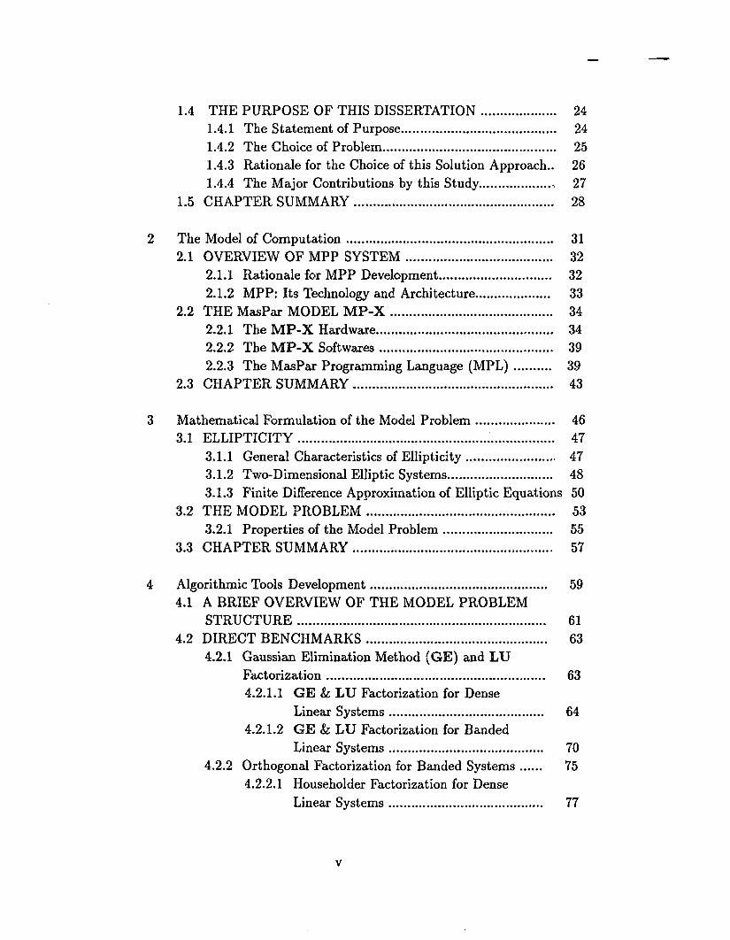
1.4 THE PURPOSE OF THIS DISSERTATION.................... 241.4.1 The Statement of Purpose............................................ 241.4.2 The Choice of Problem.................................................. 251.4.3 Rationale for the Choice of this Solution Approach.. 261.4.4 The Major Contributions by this Study.................... 27

1.5 CHAPTER SUMMARY............................ 28

2 The Model of Com putation............................................................. 312.1 OVERVIEW OF MPP SYSTEM ............................................ 32

2.1.1 Rationale for MPP Development ................. 322.1.2 MPP: Its Technology and Architecture.................... 33

2.2 THE MasPar MODEL M P - X .............................................. 342.2.1 The M P -X Hardware......................................... 342.2.2 The M P -X Softwares................................................... 392.2.3 The MasPar Programming Language (M P L ) 39

2.3 CHAPTER SUMMARY........................................................... 43

3 Mathematical Formulation of the Model P roblem ......................... 463.1 ELLIPTICITY..................................... 47

3.1.1 General Characteristics of Ellipticity........................ 473.1.2 Two-Dimensional Elliptic Systems............................. 483.1.3 Finite Difference Approximation of Elliptic Equations 50

3.2 THE MODEL PROBLEM ........................................................ 533.2.1 Properties of the Model Problem ................................ 55

3.3 CHAPTER SUMMARY...................................... 57

4 Algorithmic Tools Development.................................................... 594.1 A BRIEF OVERVIEW OF THE MODEL PROBLEM

STRUCTURE .......................................................... 614.2 DIRECT BENCHMARKS................................. 63

4.2.1 Gaussian Elimination Method (G E) and LU Factorization................................. .............................. 634.2.1.1 G E & LU Factorization for Dense

Linear System s............................................. 644.2.1.2 G E &: LU Factorization for Banded

Linear System s............................................. 704.2.2 Orthogonal Factorization for Banded System s 75

4.2.2.1 Householder Factorization for DenseLinear System s............... ...... ....................... 77

v

4.2.2.2 Householder Factorization for BandedLinear System s............................................. 79

4.3 ITERATIVE BENCHMARKS.............................................. 804.3.1 Symmetric Over-relaxation Method (SO R ) 81

4.3.1.1 The SO R Method for DenseLinear Systems.............................................. 81

4.3.1.2 The SO R Method for BandedLinear Systems................................................. 85

4.3.2 Conjugate Gradient Method (C G )................................ 874.3.2.1 The CG Method for Dense Linear Systems 89

4.4 THE NEW TECHNIQUE.................................................... 904.4.1 Recursive Doubling for Linear Recursions............... 924.4.2 Cyclic or Odd-Even Reduction ........... 95

4.5 CHAPTER SUMMARY.......................................................... 98

5 Implementations and Experimental R esults.................. 1015.1 DATA STRUCTURES............................................................ 1025.2 THE GRID CONSTRUCTION............................................. 1055.3 THE EXPERIM ENTS.......................................... 108

5.3.1 The System Size Determination and Usage.............. 1085.3.2 Exact Solution.............................................................. 1095.3.3 Experimental Approach.............................................. 110

5.4 EXPERIMENTAL RESULTS................................................ I l l5.4.1 Results and Observations........................................... 1125.4.2 Conclusion.................................................................... 125

Bibliography.................................................................................... 126

V ita .................................................................................................. 136

vi

L ist o f Tables

4.1 Operation Count of SerGE Algorithm ................................................. 67

4.2 Operation Count of SerGET Algorithm ............................................... 72

5.1 Errors of Results when n = 305, N = 93,025 ..................................... 114

5.2 Errors of Results when n = 200, N = 40,000 ..................................... 115

5.3 Errors of Results when n = 100, N = 10,000 ...................................... 116

5.4 Errors of Results when n = 40, N = 1,600 ........................................ 117

vii

L ist o f F igures

2.1 MP-X Hardware Subsystems............................................................. 34

2.2 MP-X Communication Buses............................................................. 37

3.1 Mesh Region to Approximate the Domain of the Model Problem 51

4.1 Gauss Elimination for Dense Linear Systems (SerG E)................. 66

4.2 Parallel GE and LU Factorization for Dense Linear Systems(ParGE)................................................................ 69

4.3 Gauss Elimination for Tridiagonal Systems (SerG ET)................ 71

4.4 Householder Reduction for Dense Linear System s.................. 79

4.5. Serial Jacobi Method for Dense Linear Systems (SerJAC) ............. 83

4.6 Parallel Jacobi Method for Dense Linear Systems (P arJA C ) 83

4.7 Conjugate Gradient Method for Dense Linear Systems (SerCG). 88

4.8 Recursive Doubling Technique for Linear Recursive Problems .. 94

4.9 Cyclic (Odd/Even) Reduction for the New Technique.................. 99

4.10 The New Algorithm Computing a Tridiagonal System at Various Reduction Levels................................................................................... 100

5.1 Structure of Matrix A Resulting from Model Problem, /? = n 104

5.2 The Basic Data Structures and their A llocation.............................. 106

5.3 The Mesh Region and the Mesh Point Coordinates........................ 107

5.4 The Exact Solution of the Model Problem ........................................ 113

viii

5.5 Values of U at the First 400 Grid Pointswhen n = 305, N = 93,025 ................................................................... 114

5.6 Values of U at the First 400 Grid Pointswhen n = 200, N = 40,000 .................................................................. 115

5.7 Values of U at the First 400 Grid Pointswhen n = 100, N = 10,000 .................................................................. 116

5.8 Values of U at the First 200 Grid Pointswhen n = 40, N = 1,600 ..................................................................... 117

5.9 CPU Times of the Algorithms..................... 118

5.10 Megaflop Rates of the Algorithms.................................................... 119

ix

Symbols

In the following symbol lists, the context in which some of the symbols are first

used axe indicated as the equation number the symbols are used. The equation

number in enclosed in parentheses following explanation of the symbols’ meaning.

Many symbols have multiple meanings, and, in that case, we believe the context

of their use will clear any ambiquity.

A rab ic L e tte rs

A Coefficient matrix of a system of linear equations (1.1)

A Coefficient matrix resulting from second order, n-dimensional PDE

Aij Coefficient of a partial differential of a second order, n-dimensionalPDE when the differentiation is taken with respect to vectors

Xj G IRn (3.1)

A , B, C Coefficients of second order, 2-dimensional elliptic equation whendifferentiations are taken with respect to x, y, and xy respectively (3.7)

D Diagonal matrix triangular matrix in A = U TD U (4.6)

di , . . . , d5 Diagonal vectors (5.1)

JF, / Forcing function, the right hand sides of second order, n-dimensionalelliptic equation (3.6, 3.7)

k, h Grid widths in x — and y — coordinate directions

k Right hand side (vector) of linear system of equations

L Lower triangular matrix in A = LU (4.5)

1 Reduction level (4.54)

m, n Number of partitions of mesh region in x — and y — directions

m, N Number of linear equations resulting from approximating of ellipticequation in rectangular domain; N — n2

IN" n —dimensional space (3.1)

p Diagonal matrix triangular matrix in A = U TDU(4.6)

Pi ith permutation matrix

Pi j Product of permutation matrices Pi through Pj

IBP n —dimensional space of real numbers (3.1)

Q Orthogonal matrix A = Q R (4.14)

r Residual vector

u Dependent variable of second order, n-dimensional elliptic equation (3.1)

U An approximated value of u (3.14)

U ,R Upper triangular matrix in A = LU (4.5),and in A = L U (4.14)

w Orthogonal factorization factor (4.15)

x, y , z Solution vectors (4.7,4.8)

Z Matrix such that Z = I — D _1 (4.23)

xi

G reek L e tte rs

a , /? Scalar values in Conjugage gradient algorithm, SerCG()

/3 Semi-bandwidth

ft A bounded domain

r Boundary of domain ft

V Gradient ^ , gf~p

u> Relaxation factor of SOR, SSOR, etc. 1 < < 2

p(A) Spectral radius of A

’E'i, $ 2 Sets of coordinate points in x — and y — directions

S u p ersc rip ts

At Transpose of AlnVerse of A

ith iterate, (/) being iteration level

S ubscrip ts

ajj i j th element of matrix A

v,- ith element of vector v

Pi ith permutation matrix

A bbrev ia tions

a, ja, ia substructures of the “a, ja, ia“ format of data

ACU Arithmetic control unit, a control unit of MPP

ARU Array unit, a parallel component of MPP

blk A sequence of blocks (MPL) of plural variablesseperated in memory by a fixed address increment

CG Conjugate gradient algorithm

DPU Data parallel unit of MPP performs all parallel processing

det(A) Determinant of A ()

FE Front end, a host computer of MPP

ixproc PE’s index in a:—coordinate direction, 0 < ixproc < nxproc — 1

iyproc PE’s index in y—coordinate direction, 0 < iyproc < nyproc — 1

JOR Jacobi over-relaxation method

mat A 2-dimensional array (MPL) of arbitrary size

MPL Maspax programming language, a MULTRIX C based languagefor programming MPP

MPPE Maspax programming environment of MPP

MPP Massively parallel processor of the MasPar corporation,Goodyear Aerospace.

MP-X Versions of MPP where X=1 or 2. That is, MP-X =*• MP-1 or MP-!

(sign) ±

nproc Number of PEs

nxproc Number of PEs in x —direction of PE-array

nyproc Number of PEs in y—direction of PE-array

lnproc nproc in bit representation

lnxproc nxproc in bit representation

lnyproc nyproc in bit representation

ParJAC Parallel implementation of Jacobi iterative method

ParCR Parallel implementation of cyclic reduction technique

ParCG Parallel implementation of Conjugate gradient algorithm

Par GET Parallel implementation of Gaussian elimination technique modifiedfor tridiagonal systems

ParRD Parallel implementation of recursive doubling technique

PE Processing element, a processor of MPP

PMEMSZ Size (usually in KB) of the local PE’ memory.For MP-1 (model 1208B), PM EM SZ=64tf£

plural A storage class which, when used as a part of a type attribute, causesthe datum with the attribute to be allocated on local memories of all processors. In other word, the datum effectively becomes a vector

RISC Reduced instruction set computer. The PE array of MPPis a RISC processor

ROW* A set of indices of a row of matrix A allocated on or brodcast to PE,-

SerJAC Serial implementation of Jacobi iterative method

SerCG Serial implementation of Conjugate gradient algorithm

SerGET Serial implementation of Gaussian elimination technique modifiedfor tridiagonal systems

SOR Symmetric over-relaxation method

SSOR Symmetric over-relaxation method

LSOR Line symmetric over-relaxation method

singular A storage class which which causes the datum to be allocated on ACU,thus making it be an elementary datum such as integer, character, etc.

vex A 1-dimensional array in x — major (vector) orientation

vey A 1-dimensional array in y—major (vector) orientation

xv

Abstract

This dissertation proposes a new technique for efficient parallel solution of very

large linear systems of equations on a SIMD processor. The model problem used

to investigate both the efficiency and applicability of the technique was of a regu­

lar structure with semi-bandwidth /?, and resulted from approximation of a second

order, two-dimensional elliptic equation on a regular domain under the Dirichlet

and periodic boundary conditions. With only slight modifications, chiefly to prop­

erly account for the mathematical effects of varying bandwidths, the technique can

be extended to encompass solution of any regular, banded systems. The compu­

tational model used was the MasPar MP-X (model 1208B), a massively parallel

processor hostnamed hurricane and housed in the Concurrent Computing Labora­

tory of the Physics/Astronomy department, Louisiana State University.

The maximum bandwidth which caused the problem’s size to fit the nyproc x

nxproc machine array exactly, was determined. This as well as smaller sizes were

used in four experiments to evaluate the efficiency of the new technique. Four

benchmark algorithms, two direct — Gauss elimination (GE), Orthogonal factor­

ization — and two iterative — symmetric over-relaxation (SOR) (u> = 2), the

conjugate gradient method (CG) — were used to test the efficiency of the new

approach based upon three evaluation metrics — deviations of results of computa­

tions, measured as average absolute errors, from the exact solution, the cpu times,

and the mega flop rates of executions. All the benchmarks, except the GE, were

implemented in parallel.

In all evaluation categories, the new approach outperformed the benchmarks

and very much so when N p, p being the number of processors and N the

problem size. At the maximum system’s size, the new method was about 2.19 more

accurate, and about 1.7 times faster than the benchmarks. But when the system

size was a lot smaller than the machine’s size, the new approach’s performance

deteriorated precipitously, and, in fact, in this circumstance, its performance was

worse than that of GE, the serial code. Hence, this technique is recommended

for solution of linear systems with regular structures on array processors when the

problem’s size is large in relation to the processor’s size.

xvii

Chapter 1

E xploitation o f Parallelism: Literature Survey

The more extensive a man’s knowledge of what has been done, the greater will be his power of knowing what to do.

Benjamin Disreali.

We live in a World which requires concurrency actions...- K.J. Thuber.

1.1 RATIONALE FOR PARALLELISM

A battery of satellites in outer space are collecting data at the rate of lO10 bits

per second. The data represent information on the earth’s weather, pollution,

agriculture, and natural resources. In order for this information to be used in a

timely fashion, it needs to be processed at a speed of at least 1013 operations per

second.

Back on earth, a team of surgeons wish to view, on a special display, a recon­

structed three-dimensional image of a patient’s body in preparation for surgery.

They need to be able to rotate the image at will, obtain a cross-sectional view of

cm organ, observe it in living detail, and then perform a simulated surgery while

watching its effect, and without touching the patient. A minimum processing speed

of IQ15 operations per second would make this approach feasible.

The preceding two examples are not from science fiction. They are represen­

tative of actual and commonplace scientific applications where tremendously fast

computers are needed to process vast amount of data or to perform a large num­

ber of computations in real-time. Other such applications include aircraft testing,

development of new drugs, oil exploration, modeling fusion, reactors, economic

2

planning, cryptoanalysis, managing large databases, astronomy, biomedical anal­

ysis, real-time speech recognition, robotics, and the solution of large systems of

partial differential equations arising from numerical simulations in disciplines as

diverse as seismology, aerodynamics, and atomic, nuclear, and plasma physics. No

computer exists today that can deliver the processing speeds required by these

applications. Even the so-called supercomputers peak at a few billion operations

per second.

Over the past forty years or so, dramatic increases in computing speeds were

achieved largely due to the use of inherently fast electronic components by the

computer manufacturers. As we went from relays to vacuum tubes to transistors,

and from small to medium to large to very large and presently to ultra large scale

integrations, we witness — often in amazement — the growth in size and range of

the computational problems that could be solved.

Unfortunately, it is evident that this trend will soon come to an end. The

limiting factor is a simple law of physics that gives the speed of light in vacuum.

This speed is 38 meters per second. Now, assume that an electronic device can

perform 1012 operations per second. Then it takes longer for a signal to travel

between two such devices. Why then not put the two devices together? Again,

physics tells us that the reduction of distances between electronic devices reaches

a point beyond which they begin to interact, thus reducing not only speed but also

their reliability.

It appears, therefore, that the only way around this problem is to use paral­

lelism. The idea here is that if several operations can be performed simultaneously,

then the time taken by a computation can be significantly reduced. This is fairly

an intuitive notion, and the one to which we are accustomed in organized society.

There are a number of approaches for achieving parallel computation.

3

This chapter traces the evolution of parallelism in computing systems, and

discusses the highlights of such evolution that directly impact very large scien­

tific computing problems such as the ones mentioned above. Because there has

been mainly a two-prong development in parallelism, namely, along the hard­

ware and the software fronts, the survey focuses specifically on the efforts at the

hardware and software designs which, either singly or in concert, support paral­

lelism in modern computers. §1.2 discusses parallel hardware features of modern

computers emphasing their innovative architectural designs and the influence of

means1 technologies on such designs. The three most popular classification (tax­

onomies) schemes for computers which are based upon the various architectural

aspects of the computers, and the efforts to address the deficiencies of such schemes

to adequately describe and classify some modern parallel computers, are all given

in §1.2. §1.3 treats the software parallelism emphasizing differences between par­

allel and serial algorithms, common methodologies and essential design steps for

creating parallel algorithms, the characteristic features of parallel algorithms, and,

lastly, the parallel algorithms ranging from the previously proposed to the most

recent ones that are available for efficient solution of a broad spectrum of scien­

tific problems. Based upon the information gained from the studies covered in

this literature survey, an effort will be undertaken to design efficient algorithms

for the type of problem that this dissertation sets out to solve in accordance with

the purpose of this study as succinctly explained in §1.4. The chapter summary is

given in §1.5.

1In computer architecture, the word technology refers to the electronic, physicochemical, or mechanical for the entire range of implementation techniques for processors and other components of computers.

4

1.2 HARDW ARE PARALLELISM

1.2.1 The G enesis o f High-Perform ance Com puters

Spurred by the advances in technologies, the past four and a half decades have

seen a plethora of hardware designs which have helped the computer industry to

experience generations of unprecedented growth and development which have been

physically marked by a rapid change of computer building blocks from relays and

vacuum tubes (1940 - 1950s) to the present ultra-scaled integrated circuits (ICs)

[HOCK 88, GOLUB 93, DUNCAN 90, STONE 91].

As a result of these technological advances and improved designs, computer

has undergone a remarkable metamorphosis from the slow uniprocessors of the

1950s to today’s high performance machines which include supercomputers whose

peak performance rates are thousands order of magnitude over those of earlier

computers [HWANG 84, STONE 80, HOCK 88, HAYNES 82]. The requirements

of engineers and scientists for ever more powerful digital computers have been

the main driving force in the development of digital computers. The attain­

ment of high computing speeds has been one of the most, if not the most, chal­

lenging requirement. The computer industry’s response to these challenges has

been tremendous, and the result is the remarkable evolution in computers in just

three short decades (1960s to 1980s) as exemplified by an existence of commercial

and experimental high-performance computing systems produced in these decades

[HELLER 78, GOLUB 93, MIRAN 71, STONE 90, HWANG 89]. The quest for

even more powerful systems for sundry scientific applications such as are mentioned

above continues unabated into the 1990s.

5

1.2.1.1 T h e E a rly C o m p u ters

The early computers were not powerful because they were designed with much

less advanced technology compared to what we have today. The first electronic

computer was ENIAC. It was designed by the Moore School Group of University

of Pensylvania in 1942 to 1946. ENIAC had no memory and it was a stored-

program computer. That is, a program had to be manually loaded through external

pluggable cables. ENIAC, like all other early computers, especially those of the late

1930s through 1940s (e.g., the first electronic computer built in 1939 by Atanosoff

[MACK 87] to solve matrix equations), was very crude and had a very limited

computational capability that is not even a match to that of some of today’s hand

calculators. For example, the computer by Atanosoff could solve matrices of order

up to only 29 whereas some calculators can compute matrices of a lot higher orders

than 29.

Very soon after the ENIAC design was frozen in 1944, von Neumann2 Be­

came associated with the Moore School Group as a consultant, and the design of

EDVAC3, which was already underway, proceeded full steam. The basic design of

EDVAC, as outlined in the very widely publicized momerandum authored by von

Neumann [VON 45], consisted of a memory ” organ” whose ” different parts” could

perform different functions (e.g., holding input data, immediate results, instruc­

tions, tables). Thus with EDVAC was born the stored-program concept with a

homogeneous multifunctional memory.

The later variation of the stored-program concept became the underlying princi­

ple for design of many computers from 1950s until today. The architectural designs

of many familiar systems ranging from the early uniprocessors (e.g., IBM 2900)

2A Hungarian born mathematician (1903 - 1957).3EDVAC was the immediate successor of ENIAC.

6

of the 1950s to the contemporary systems (e.g., IBM System/370, and the 4300

family [SIEWIO 82], the DEC VAX series, namely, VAX 11/750, 11/780, and 8600

[DIGIT 81a, DIGIT 81b, DIGIT 85], and the Intel 8086 [MORSE 78], etc.), are all

based upon this design principle. This principle is known as the von Neumann ar­

chitecture even though von Neumann became associated with the ED VAC design

team only after the design had already begun. A storm of controversy over this mo­

nopolistic claim has been raging since the 1940s mainly because no other members

of the design team, not even Eckert and Mauchly who were the chief architects of

both ENIAC and EDVAC, received any credit4 for the ENIAC design. For detailed

treatment of the stored-program concept, how the concept came to be associated

with only von Neumann, and the controversy that has been ensuing as the result

of that association, see the publications by Wilkes [WILKES 68], Metropolis and

Whorlton [METRO 80], Randell [RAND 75], and Goldstine [GOLD 72] (Part 2).

For the von Neumann architecture, its characteristic features and deficiencies (e.g.,

the notorious bottleneck due to mainly the monolithic memory access), as well as

the modern architectural means5 of overcoming these deficiencies, see the texts by

Stone [STONE 90], and Dasgupta [DASGUP 89b]. Our only concern here is to

emphasize the fact that ENIAC, EDVAC, and other early computers were very

slow, awkward, and with a capability to compute only the most elementary nu­

merical problems the like of which is nothing compared with the type of problems

mentioned in the beginning of this chapter.

4The von Neumann’s 1945 memorandum contained neither references to nor acknowledgement of other members of the EDVAC design team.

5In fact, the existence of a number supercomputers are attributable to overcoming these deficiencies.

7

1.2.1.2 The Role of Technology and Innovative Design Philosophies

The two most obvious factors responsible for the crude and rudimentary nature

of the early computers were that the components of these computers were con­

structed from slow and bulky vacuum tubes and relays as switching devices, and

the fact that the computer design then was at its infancy and, therefore, lacked

the touch of sophistication of today’s design. The needed touch of sophistication

and the influence that touch would have over the computer designs in the fol­

lowing decades, and the culmination of those designs in today’s high-performance

computers, awaited the invention of a better technology.

That invention was a fast solid-state binary switching device known as tran­

sistor. Transistor was invented in 1947 by three American physicisists — John

Bardeen, Walter H. Bratain, and William B. Shockley — at the Bell Telephone

Laboratories. Transistors are the building blocks of integrated circuits (ICs), the

basic components of modern computers. The first discrete transistors were used

in the digital computers about 1959. Since then, there has been dramatic im­

provement in the computational power of digital computers. Such improvement

has been proceeding hand in hand with advances in mostly the silicon-based tech­

nologies evidenced in the reduction of chip’s feature size and IC miniaturization6

which results in significant increases in IC integration levels7. These and similar

technological advances have led to decrease in cost of hardware components (e.g.,

memory) while improving their performance. More than anything else, it is the

improvement in the hardware technology which has been responsible for transform­

ing the slow uniprocessors of the earlier decades to the high-performance machines

of the 1980s to 1990s. For full discussion of computer technologies and relevant

6Examples: Bipolar Transistors (TT1, ECL, I2L) and Field-effect Transistors ( NMOS, PMOS, HMOS, CMOS - CMOS-1, CMOS-2, CMOS-3, CMOS-4), GaAs MESFETs).

7The number of logic gates or components per IC.

8

topics, see chapter 1 of the book by Dasgupta [DASGUP 89a], and the paper by

Hollingsworth [HOLL 93].

1.2.1.3 A Breed of M odem High-Performance M achines

The above transformation has also been accelerated by revolutionary design, which

often occured in tandem with improved technology. The commonnest design tech­

nique has been to incorporate some parallel features into the modern computer.

Since the 1960s, literally hundreds of highly parallel structures have been proposed,

and many have been built and put into operation by the 1970s. The Illiac IV was

operational at NASA’s Ames Research Center in 1972 [BOUK 72] ; the first Texas

Instrument Inc. Advanced Scientific Computer (TI-ASC) was used in Europe in

1972 [GOLUB 93]; the first Control Data Corp. Star-100 was delivered to Lawrence

Livermore National Laboratory in 1974; the first Cray Research Inc. Cray-1 was

put to service at Los Alamos National Laboratory in 1976.

The machines mentioned immediately above not only were the pioneers in inno­

vative designs which have endowed these machines with an unprecedented power,

but were also the fore-runners of even more powerful computing systems yet to

come. Therefore, while their fames were still undimmed, they soon gave way to

other generations of more powerful computers which culminate in today’s super­

computing systems. Thus by 1980’s, a substantial number of high-speed processors

of the 1960s and 1970s either ceased to be operational or played less significant

computing role while, in the same decades, the advance of the processing speeds

and the improvement in the cost/performance ratio — an important design met­

ric — continued unabated. The overall result were the introduction of new and

more radical8 architectural design philosophies such as evidenced in the reduced

8Vis a vis Von Neumann architecture.

9

instruction-set computers (RISC), a widespread commercialization of multipro­

cessing, and the launching of the initial releases of massively parallel processors.

Thus Uliac-IV ceased operation in 1981; TI-ASC is no longer in production since

1980; since 1976, the Star-100 has evolved into the CDC Cyber 203 (no longer

in production) and also into the Cyber 205 which signaled the CDC’s entry in

the supercomputing field; the Cray-1 (pipelined uniprocessor) has evolved into

Cray-IS which has considerably more memory capacity than the original Cray-1,

Cray-XMP/4 (4-processor, 128 MWord supercomputer with peak performance rate

of 840 MFLOPS), Cray-2 (256 Mword, 4-processor reconfigurable supercomputer

with 2 GFLOPS peak performance), Cray-3 (16-processor, 2 GWord supercom­

puter with 16 GFLOPS peak performance rate). Other superperformance com­

puters produced in the 1980s include Eta-10, Fujitsu VP-200, Hitachi S-810, IBM

3090/400/VF, and a hoste of others (see chapter 2 of [HWANG 89], also note the

influence of technologies on the design of these systems). Thus, by 1980s, the high­

speed processors of the 1960s to 1970s have evolved in the supercomputers of the

1980s through 1990s, otherwise, totally new breed of high-performance machines

were born.

Other computers of some historical interest, although their primary purpose

was not for numerical computation, include Goodyear Corporation’s STARAN

[GOODYR 74, GILM 71, RUDOL 72, BATCH 74], and the C.mmp system at

Carnegie-Mellon University [WULF 72]. Also of some historical interest, although

it was not commercialized, is Burroughs Corporation’s Scientific Processor (CSP)

[KUCK 82].

10

1.2.1.4 T h e A dvent o f A rray P rocesso rs

The Illiac IV had only 64 processors. Other computers consisting of a large (or po­

tentially large) number of processors include Denelcor HEP and the International

Computers Ltd. Data Array Processor (ICL DAP), both of which are offered com­

mercially, and a number of one of a kind systems in the various stages of completion

[GOLUB 93, HOCK 65]. These include the Finite Element Machine at NASA’s

Langley Research Center; MIDAS at the Lawrence Berkeley Laboratory; Cosmic

Cube at the California Institude of Technology; TRAC at the University of Texas;

CM* at Carnegie-Mellon University; ZMOB at the University of Maryland; Pringle

at the University of Washington and Purdue university; and the Massively Parallel

Processor (MPP) at NASA’s Goddard Space Flight Center. Only a few (e.g., MPP,

ICL DAP) are designed primarily for numerical computation while the others are

for research purposes.

1.2.1.5 T h e F u tu re of H igh-P erfo rm ance C o m p u te rs

Thus without a doubt, the 1970s to 1980s saw a quantuum leap in computer

designs which embody parallel features for high performance capabilities. The

need for ever faster computers continues into the 1990s. Every new application

seems to push the existing computers to their limit. So far, the computer man­

ufacturers have kept up with the demand admirably well. But will the trend

continue beyond the 1990s? We think it will but that, as previously surmised,

the trend will be tempered somewhat, if not completely checked, in a not-too-

distant future, unless we seek other avenues9 to find other means and techniques

of improving upon the future high-performance computing systems. These means

include new technologies, more radical or exotic designs, and software parallelisms.

9Other than silicon-based technologies.

11

Experts in computer-related traditions — hardware and software designers, tech­

nology inventors, etc. — are upbeat in expectation, otherwise, are near-unanimous

in their agreement concerning the future of high-performance computations (see

Stone et al. [STONE 90, STONE 91, DASGUP 89a, DASGUP 89b, DUNCAN 90,

HENSY 91, HAYNES 82, BATCH 74]). The above listed alternatives as well as

other means for improving the the performance of the future systems must be

aggressively pursued because, as noted in §1.1, the present largely silicon-based

technologies have a number of limitations — the pin-limitation, speed-limitation of

metal interconnection, chip’s feature size limitation, integration limitation, and the

package density limitation — which are not likely to be overcome in the foreseeable

future. Since the insatiable taste of scientists and engineers for high-performance

machines with more and more capabilities is not likely to be slaked with any wait

for the limitations of the present technologies to be overcome, a clarion call is

sounded for immediate pursuit of these other means. Fortunately, according to

the literature, the call has been answered and, as a result, other means and tech­

niques (new technologies, pipelining, cache and parallel memories, RISC ideas,

various topologies of processors in the multi-processor systems, efficient method­

ologies for design of parallel softwares, etc. ) are already involved in the design

of tomorrow’s supercomputers. If this effort continues, and we are hopeful that it

will continue, then we are more than likely to be blessed with future generations of

supercomputers which will be capable of performing mind-boggling computational

feats hardly envisioned today.

1.2.2 M odels o f Com putations and their Classifications

As noted in §1.1.1, the decades of the 1960s through 1990s have witnessed the intro­

duction of a wide variety of new computer architectures for parallel processing that

complement and extend the major approaches to parallel computing developed in

12

the 1960s and 1970s. The recent proliferation of parallel processing technologies

has included new parallel hardware architectures (systolic and hypercube), inter­

connecting technologies (multistage switching topologies). The sheer diversity of

the field poses a substantial obstacle to comprehend what kinds of parallel architec­

tures exist and how their relationship to one another defines an orderly schema. We

examine below the Flynn’s taxonomy which is the early and still the most popular

attem pt at classifying parallel architectures and then give brief summary of the

more recent classification schemes proposed to reddress the inadequacy of Flynn’s

taxonomic scheme in order to unambiguously include all parallel processors, both

the old and the modern, into proper taxa.

1.2.2.1 F lynn’s Taxonomy

Flynn’s taxonomy [FLYNN 66, FLYNN 72] classifies architectures based on the

presence of single or multiple streams of instructions and data into the following

categories:

» SISD (single instruction, single data stream) — defines serial computers with

parallelism in neither data nor instruction stream.

9 SIMD (single instruction, multiple data stream) — involves multiple proces­

sors under the control of one control processor simultaneously executing in

lockstep the same instruction on different data. Thus a SIMD architecture

incorporates parallelism in data stream only.

9 MISD (multiple instruction, single data stream) — involves multiple proces­

sors applying different instructions to a single data stream. MISD exhibits

parallelism only in the instruction stream.

13

• MIMD (multiple instruction, multiple data stream) — has multiple proces­

sors applying different instructions to their respective data streams thus ex­

hibiting parallelism in both the instruction and the data streams.

1.2.2.2 O th e r Taxonom ies

Although the Flynn’s taxonomy provides a useful shorthand for characterizing

computer architectures, it is insufficient for classifying various modern computers.

For example, pipelined vector processors merit inclusion as parallel architectures,

since they exhibit substantial concurrent arithmetic execution and can manipulate

hundreds of vector elements in parallel. However, they can not be regarded as any

of the Flynn’s taxa because of the difficulty to accomodate them into the taxon­

omy as these computers lack processor that execute the same instruction in SIMD

lockstep and fail to possess the autonomy of the MIMD category. Because of the

deficiency of the Flynn’s taxonomy, attempts have been made to extend the Flynn’s

taxonomy to accomodate modern parallel computers. There are other taxonomies

which are distinctively different from the Flynn’s mainly because they are based

upon criteria different from those of the Flynn’s taxonomy. Among the best known

of these taxonomies are those by Handler [HAND], Giloi [GILOI 81, GILOI 83],

Hwang and Briggs [HWANG 84, HWANG 87], and Duncan [DUNCAN 90]. But

these taxonomies generally lack the simplicity inherent in the Flynn’s, and, conse­

quently, they are not as widely used as the Flynn’s. We give below a brief summary

of the distinctive features of these taxonomies here and refer the interested readers

to the works of Mayr [MAYR 69], Hockney [HOCK 87] , Ruse [RUSS 73] , Sokal

and Sneath [SOKAL 63], Dasgupta [DASGUP 89b], and Skillcorn [SKILL 88], for

in-depth treatments of these taxonomic schemes.

1.3 SOFTW ARE PARALLELISM

14

The treatment so far exposes the existence of parallelism at the hardware level as a

direct result of the advances in technologies and the improvement of architectural

designs of the modern computers. One may be tempted to conclude that in or­

der to realize more parallelism and, therefore, achieve greater computational power

from a computer, one has to use faster technologies (circuits) or use more advanced

architectures. As noted in §1.1.1, the improvement in these areas have been im­

mense. However, as also noted in that section and by Dasgupta [DASGUP 89a],

the design of circuits have some limitations which naturally militate against much

additional gains in parallelism realizable from the hardware. Therefore, any signif­

icant additional improvement must be sought elsewhere such as the software arena.

There are a number of efficient parallel algorithms proposed for solution of practi­

cal and experimental scientific problems. These are well documented in the litera­

ture. Among the early excellent surveys on such algorithms are those of Miranker

[MIRAN 71], Traub [TRAUB 74], Voigt [VOIGT 77], and Heller [HELLER 78].

The more recent such surveys include that by Ortega [ORTEGA 85].

1.3.1 D esirable Features o f a Parallel A lgorithm

The challenge posed by software parallelism is to devise algorithms and arrange

computations to match the features of the algorithms to match those of the under­

lying hardware in order to maximize parallelism. As noted by Ortega and Voigt

[ORTEGA 85], some of the best known serial (sequential) algorithms turn out

to be unsatisfactory and need some modifications or even be discarded while, on

the other hand, many older algorithms which had been thought to be less than

optimal on serial machines have had rejuvenation because of their inherent paral­

lel properties. Also, the current researches in parallel computation indicate that

15

we can not directly apply our knowledge of serial computation to parallel com­

putation because efficient sequential algorithms do not necessarily lead to efficient

parallel algorithms. Moreover, there exist several problems perculiar to parallelism

that must be overcome in order to perform efficient parallel computations. Stone

[STONE 73] and Miklosko [MIKLOS 84] cite these problems as being:

1. Efficient serial algorithms are not necessarily efficient for parallel comput­

ers. Moreover, inefficient serial algorithms may lead to efficient parallel al­

gorithms.

2. Data in parallel computers must be arranged in memory for efficient parallel

computation. In some cases, the data must be rearranged during the execu­

tion of the algorithm. The corresponding problem is nonexistent for serial or

sequential computers.

3. The numerical stability, speed of convergence, cost, and the complexity anal­

ysis of serial and parallel algorithms can be different.

4. Serial algorithms can have severe constraints that appear to be inherent, but

most, if not all, can actually be removable.

What all this means is that

1. an efficient parallel algorithm is not a trivial extension of an efficient serial

counterpart, but that it may be necessary to identify and then eliminate the

essential constraints that are perculiar to the serial algorithm in order to

create the parallel algorithm,

2. each of different parallel architectures (SIMD, MIMD, etc. ) requires a change

in the way a programmer formulates the algorithm and develops the under­

lying code. The programmer must establish a sensitivity to the underlying

16

hardware architecture he/she is working with to a degree unprecedented in

serial computers. An efficient and effective parallel algorithm exploits the

strengths of the underlying hardware while de-emphasing its weaknesses,

3. suitable data structures (static and/or dynamic) and appropriate mapping

of the data structures onto a parallel run-time environment, also, the inter-

processor communication, are all indispensable for efficient parallel program­

ming. Because this mapping of data is usually more complicated than solving

the problem itself, there have been some successful efforts in automating the

process. Geuder, et al. [GEUDER 93], Levesque [LEVES 90], for example,

have proposed and designed a software dubbed GRIDS which has been used

by Lohner [LOHNER 93] to provide the user an interface for automatic map­

ping of his/her program structures to parallel run-time components.

1.3.2 D efinition o f a Parallel A lgorithm

At any stage within an algorithm, the parallelism of the algorithm is defined as

the number of arithmetic operations that are independent and, therefore, can be

performed concurrently (simultaneously). On a pipeline computer, the data for

operations are commonly defined as vectors, and a vector operation as a vector

instruction. The parallelism is then the same as the vector length. On array pro­

cessors, the data for each operation are allocated on different processors (commonly

known as processing elements or PEs), and operations on all PEs are performed

at the same time, but with different data, but under the control of the master

control processor. The parallelism is then the number of data elements operated

upon simultaneously. In MIMD computers, the number of processors involved in

asynchronous computation of a given problem is the parallelism.

17

Natural parallelism is present mainly in the algorithms of linear algebra and

in the algorithms for the numerical computation of partial differential equations.

It is also present in algorithms that are based on the iterative computation of

the same operator over different data, e.g. identical computations dependent on

many parameters, method of successive approximations, some iterative methods for

solving systems of linear equations, Monte Carlo methods, numerical integration,

and in complex algorithms which consist of a large number of almost independent

operators, e.g. iterative computation of Dirichlet’s problems by the difference

methods, the finite difference methods.

There are some parameters which are often used for accessing the performance

of parallel algorithms. These include the running time, T, speedup, S, cost or

work, complexity, number of processors, n. The definition of these and other

relevant metrics are given with respect to various underlying parallel hardwares by

Lambiotte [LAMBIO 75], Ortega [ORTEGA 85, ORTEGA 88, GOLUB 93], Heller

[HELLER 78], Leighton [LEIGH 92], Aki [AKI 89], Voigt [VOIGT 77], and Eager

et al. [EAGER 89].

1.3.3 Comm on M ethods for Creating Parallel A lgorithm s

There are a number of procedures for efficient design of serial algorithms, and most

of these naturally carry over to the design of parallel algorithms. Most parallel

algorithm constructions follow one or more of the following approaches:

1. method10Restructuring of a numerically equivalent parallel algorithm from a

given serial algorithm.

2. Divide-and-Conquer which recursively splits a given problem into subprob­

lems that are solved in parallel.

10Also called reordering by some authors.

18

3. Vectorization of the internally serial algorithm in which a given direct serial

algorithm is converted to an iterative method which rapidly converges to the

solution under certain conditions.

4. Asynchronous parallel implementation of a serial, strictly synchronized algo­

rithm.

We note that methods 1 and 2 have also been used to render serial computations

effective; but methods 3 and 4 are new and are only suitable for parallel compu­

tations. Method 1, for example, has been used for enhancement of parallelism of

arithmetic expressions in mathematical formulae by exploiting associative, commu­

tative, and distributive laws of computation [MURA 71, KUCK 77]. Restructuring

is also often applied to reorder the computation domain or the sequence of opera­

tions in order to increase the fraction of the computation that can be executed in

parallel. For example, the order in which mesh points on a grid are numbered can

increase or decrease parallelism when solving elliptic equation. Method 2 is usually

applied to realize parallelism in numerical computation of initial value problems

of, say, ordinary differential equations. The algorithms described by Nievergelt

and Pease [NIEVER 64, PEASE 74] consist of multiple parallel applications of a

numerical method for solving many initial value problems. The divide-and-conquer

method (see the excellent treatment of this topic by Grit and McGraw [GRIT 88]

for MIMD architecture) is widely used for computation on both SIMD and MIMD

computers. A good example of algorithm which lends itself to the application of

divide-and-conquer principle is the inner product computation X) a i «> where the

product a,-6,- can be computed by processor p,. This might involve sending a,+l

and 6,+i to p.- for i odd. The sum operation is now "divided” among p/2 pro­

cessors with pi doing the addtion a,&i + ai+ibi+i for i odd. The idea is repeated

logn times until the sum is "conquered” in processor p,-. Mehod 3, vectorization

19

method, is usually applied to accelerate vector solution of numerical problems and

are particularly effective for executiing on SIMD vector processors. Method 4 is

often used for designing parallel algorithms, and its application is demonstrated

by Miranker and Chazan [MIRAN 71, CHAZAN 69] using the so-called chaotic

or asynchronous implementation of parallel solution of linear system arranged as

x = A x + b.

1.3.4 Parallelism in N um erical A lgorithm s

Enormous research efforts have been expended in exposing and exploiting software

parallelism. Efficient parallel algorithms have been created by reformulating the

existing serial algorithms and by creating new ones for solution of problems from ar­

eas of sciences as diverse as fluid dynamics, transonic flows, reservoir simulations,

structural analyses, mining, and weather prediction, and computer simulations.

There have been remarkable progress in designing software for solving problems

in all facets of scientific applications due to several favorable factors che chief of

which being the advancement in and availability of parallel computing technology

(hardware and software). In the area of computer simulation, for instance, much

has been achieved. Such a success is exemplified by such ambitous attem pt at

developing a very large-scale Numerical Nuclear Plant (NNP) by the Reactor Sim­

ulation and Control Laboratory (RSCL) team at the Argonne National Laboratory

(ANL) [TENT 94]. NNP will simulate the detail response of nuclear plants to a

number of specified transients. Below, we give a brief summary of the parallel

algorithms which are commonly utilized in solving systems resulting from many

scientific applications.

20

1.3.4.1 M atrix/V ector Algorithm s

Since the invention of the first electronic computer by Atanasoff to solve ma­

trix equations of order 29 in 1939, researchers in many scientific and engineering

disciplines have found their problems invariably reduced to solving systems of

simulataneous equations that simulate and predict physical behaviors. Hardly is

there any area of scientific applications in which are matrix and vector manip­

ulations are not involved in one form or the other in developing algorithms for

solutions of the problems. Little wonder, therefore, that a good number of these

algorithms include a variety of data structures for memory allocation of matri­

ces and vectors in order to facilitate processor-processor data routing necessary

for efficient manipulation of matrices and vectors. Such include algorithms for

matrix-matrix multiplication, matrix-vector multiplication, matrix transpose and

inverse, eigenvalues, spectral problems, etc. (see text books with excellent treat­

ments of these and other relevant topics by Aki [AKI 89] and Modi [MODI 88])

Aki and Modi have given these algorithms for computation on different kinds of

parallel architectures of various topologies — MIMD and SIMD (tori, and tree-,

mesh-, shuffle-, cube-, and ring-connected). Leighton [LEIGH 92] has extended

the treatment to include other architectures such as systolic machines. Hockney

and Jesshope [HOCK 88] have given a parallel matrix-matrix multiplication for

execution on mesh-connected SIMD (ECL DAP) architecture and concluded that

the maximum parallelism of O(n) is realizable with outer-product algorithms, that

the outer-product method is, therefore, suitable for array processors, and that the

maximum parallelism is possible if the dimension n x n of the matrices match

the processor array. When such a match is not possible, they have proposed a

combination of techniques with which parallelism as much as n3 results. Heller

[HELLER 78] recommends inner-product matrix-matrix multiplication algorithms

21

for vector computers on the ground that the inner-product is generally included

among the hardware operations of many vector computers, and that the use of

such built-in hardware operations will not only make the algorithm efficient and

robust but will also save the start-up time.

1.3.4.2 Linear System s

Parallel solutions of arbitrary linear systems, expressed in a vector-matrix form as

A x = b, (1.1)

are of very practical importance in all branches of science where they have been

extensively used. Therefore, much research work has been directed to finding so­

lutions of solving linear systems. Linear systems are the most heavily investigated

area as far as parallel computations are concerned, and a good many parallel solu­

tions have been developed. Lambiotte [LAMBIO 75] covers many parallel solution

approaches with respect to the CDC STAR. Ortega [ORTEGA 88] has given a

report of a survey in which an extensive overview of parallel algorithms commonly

used for solving linear systems in many areas of sciences is included, and, in the

text book [ORTEGA 85], he has treated a large number of parallel algorithms for

solution of linear systems on mainly SIMD and vector architectures. Hockney and

Jeshoppe [HOCK 88] have given similar solutions but with respect to only array

processors (ECL DAP). Hockney [HOCK 81] has developed a number of efficient

algorithms for solution of spectral problems resulting from simulation of particles.

Parallel solution for the linear systems include such typical topics as the various

elimination and factorization techniques, Fast Fourier Transforms, FFT, which

are commonly employed in developing serial algorithms, as well as topics such as

cyclic reduction, recursive doubling which are presently used exclusively as paral­

lel solution techniques. Any parallel solution developed for a general dense linear

22

system must, of necessity, be modified before it can used to solve a sparse sparse

systems. The nature and extrent of the modification, of course, depend on the

given sparse system. That is, whether it is banded (e.g., triangular, tridiagonal,

pentadiagonal, etc.) or nonbanded (e.g., sparse systems with nonregular structures

such as a skewed-Hermitian system or those with almost regular structures such

as a Toeplitz system, etc.). For example, cyclic reduction and recursive doubling

methods mentioned above are generally used for developing parallel algorithms

for symmetric positive definite linear systems. For other types of systems, these

methods must be modified or different methods are developed for their solution.

Sun [SUN 93a] has proposed an efficient simple parallel prefix (SPP) algorithm for

solution of almost Toeplitz system on array processor11 and on Cray-2 supercom­

puter, and another algorithm [SUN 93b] , the parallel diagonal dominant (PDD)

algorithm for symmetric and skewed-symmetric Toeplitz tridiagonal systems, the

efficiency of which algorithm was tested on an Intel/860 multiprocessor. Garvey

[GARVEY 93] has proposed a new method for the solution of the eigenvalue prob­

lem for matrices having skewed-symmetric (or skewed-Hermitian) component of

low rank, and shows that it is faster than the established methods of compara­

ble accuracy for the general unsymmetric n x n matrix provided the rank of the

skewed-symmetric component is less than

Most of the techniques for solving linear systems are direct rather than iterative.

Some iterative methods such as Jacobi display some parallelism in that evaluation

of new iterates can be carried out with simultaneous substitutions of the old ones

thus giving a maximum parallelism of O(n). But Jacobi technique is not recom­

mended for parallel computation because of its notoreity for a slow convergence

rate. But the Jacobi method has been a foundation of other iterative techniques

with accetable convergence rates. These include successive over-relaxation (SOR)

“ MasPar MPP.

23

method and its variants such as successive line over-relaxation (SLOR), symmetric

successive over-relaxation (SSOR), the Chebychev SOR and block SOR. Other iter­

ative techniques with good convergence rates are the alternating direction implicit

(ADI), preconditioned conjugate gradient (PCG) methods.

Treatments of utilization of these iterative approaches for parallel solution of

linear systems are given by Ortega [ORTEGA 85], Lambiotte [LAMBIO 75], Bau-

comb [BAUCOM 88]. Lambiotte carries out investigations for parallel solution of

very large linear systems with repeated right hand sides. In particular, he has devel­

oped efficient parallel solution of large linear systems on the CDG 100 (vector pro­

cessor) using both direct and iterative techniques under different storage schemes.

Beacomb has also investigated the parallel solution of similar systems (that is, very

large linear systems arising from self-adjoint elliptic systems) using a MIMD com­

puting model — the Alliant FX/8 multiprocessors. She applied the preconditioned

conjugate gradient method and its several variants such as reduced12 system con­

jugate gradient (RSCG), diagonal-scaled reduced conjugate gradient (DRSCG),

incomplete Choleski reduced system conjugate gradient (ICRSCG). Other inves­

tigators who have devised and used parallel algorithms to solve similar systems

include Hockney [HOCK 65],hockney88) who designs an efficient direct method

which uses a block cyclic reduction and FFT in a rectangular mesh domain to

solve a Poisson equation with periodic and Dirichlet boundary conditions on the

IBM 7090 computer. Swarzttrauber [SWARZ 89], Sweet [SWEET 73], Schumann

and Sweet [SCHUM 76], Buzbee, et al. [BUZBEE 70], have extended the Hockney’s

solution approach in a variety of ways to encompass solution of elliptic equation

with periodic, Dirichlet and Neumann boundary conditions in either regular or

irregular domains. Recently, similar studies on sparse systems have been carried

out by Anderson [ANDER 89], Golub [GOLUB 93], and Sweet [SWEET 93].

12Reductions with red-black, Cuthill-McKee reordering.

24

1.4 THE PU R PO SE OF THIS DISSERTATION

Armed with the knowledge gained from this literature survey of the various studies

of both the hardware and the software parallelism, we now demonstrate how this

knowledge will be exploited in our quest for efficient softwares to solve the kind of

problem that this dissertation sets forth to solve. The description of the problem

and the ways and means of solving it are the major topics of treatment in the

following section.

1.4 .1 T he Statem ent of Purpose

This dissertation has a three-fold purpose which is summarized in the following

steps:

Step 1: Develop an efficient parallel algorithm based upon the cyclic reduction and

recursive doubling techniques to solve large linear system such as given in eq .(l.l).

The model of this problem will be developed in chapter 3. The iteration steps of

the cyclic reduction component of this method will be carried out to the maximum

reduction level of [log2 N~\ — 1, where N is the size of the system. The recursive

doubling step will solve the system resulting from that reduction process using

the LU factorization technique and the removal by parallel means any recursions

which occur during the factorization.

Step 2: Develop parallel algorithms baaed upon the following direct approaches:

• Direct methods — Gauss Elimination (GE), LU and Orthogonal factoriza­

tions,

• Iterative methods — Symmetric Over-relaxation (SOR), Conjugate Gradi-

ent(CG) techniques.

25

Step 3 : Solve the model problem using the parallel algorithm of steps 1 and 2

on an array processor, the MasPas MP-X whose architecture and software specifi­

cations are described in chapter 2, and use the solutions from step 2 methods as

the benchmarks to evaluate the efficiency of step 1 solution. The computational

model for the execution of the above proposed algorithms is MasPar MP-X model

1208B, and its architectural and software features will be treated in chapter 2. The

characteristics of the system to be solved and the relevance of those characteristcs

in developing the mathematical model of the problem will be extensively covered

in chapter 3. The development of the parallel algorithms suggested in Steps 1

and 2 will be covered in detail in chapter 4. Such coverage will, of course include

design of appropriate data structures for efficient data routings and other intra-

and inter-processor communications necessary for the efficient implementation of

the algorithms. Steps 3 treatment will be elaborated in chapter 5. The results of

and the conclusion on the investigations proposed in step 3 will be given in chapter

5. Finally, chapter 6 will propose potential future research work based upon this

study.

1.4.2 The Choice o f Problem

The linear system of equations, such as depicted in eq. (1.1), is the problem chosen

for solution in accordance with the statement of the purpose given above. This

kind of system occurs very frequently and often as a result of some mathematical

modeling of certain problems in every scientific discipline. But in the context

of this study, we will confine the linear systems to those resulting from elliptic

problems in regular domain and with Dirichlet boundary conditions. Moreover,

the linear system is assumed to be very large, highly sparse, and with regular

structures. Examples of such systems include banded linear systems with semi­

bandwidth of, say, /3. The most widely studied members of the family of these

26

problems include tridiagonal, pentadiagonal, and Toeplitz systems. These sure the

type of systems solved by Lambiotte [LAMBIO 75], Baucomb [BAUCOM 88] and

many other investigators on various parallel machines.

1.4.3 R ationale for th e Choice o f th is Solution Approach

Our choice of cyclic reduction methodology for the parallel solution of the linear

system is based upon the following reasons:

1. Cyclic reduction and its variants has been one of the most preferred methods

for solving general linear systems (dense & sparse), and it is particularly

efficient for solving linear systems with certain properties such as sparsity

and regularity of structures, the type serve as the model for this study. Cyclic

reduction, when used in combination with other techniques, has been heavily

applied for solving these types of systems.

2. Although it was originally developed (see brief disscussion below) with no

parallelism in mind, cyclic reduction has considerable inherent parallelism.

3. Cyclic reduction is also known for its superior numerical stability.

Cyclic reduction was originally proposed for the general tridiagonal systems by

G. Golub and developed by R. Hockney for special block tridiagonal systems

[HOCK 65]. In that work, Hockney used the method of cyclic reduction in com­

bination with a Fourier analysis to solve a linear system resulting from a model

of a particle-charge problem on a rectangular mesh region of 48 x 48 on the IBM

7090. This method was known as FACR. Since then, this approach and its sev­

eral variants13 have been successfully and efficiently applied by a number of in­

13Variants, given as FACR(l), are based on reduction to level /.

27

vestigators for the solution of linear systems resulting from elliptic systems (see

[SWEET 73, SWARZ 89, SCHUM 76, HOCK 70, GOLUB 93, SWEET 93]).

The technique of cyclic reduction has been traditionally used in conjunction

with the serial Gauss Elimination (GE) technique for solution of the reduced sys­

tem which results from the iterative reduction process using the cyclic reduction.

Searching through the past and the current literature, no one has proposed any

study nor designed an algorithm which involves the two techniques for solving a

big linear system of equations. Given this parallel feature of the recursive doubling

and our suspicion that this technique may be more efficient in terms of speed than

the serial GE method, we propose a methodology comprising of these two powerful

solution tools to solve the type of linear problems to be modeled for this study, and

to have the problems solved on an array processor. We call this new methodology.

The efficiency of this technique will be tested against the performances of some

of the classical techniques (see above for their listing) for solving linear systems.

Most of the algorithms involved will be implemented in parallel.

1.4.4 T he M ajor Contributions by this Study

Although, as indicated above, the cyclic reduction has been widely applied for par­

allel solution of systems of linear equations, there is no report in the literature on

major studies undertaken to specifically compare the computational merits of the

classical methodologies traditionally applied for solution of large linear systems,

such as to be used for investigation in this study, when such methodologies are used

in conjucntion with cyclic reduction technique to solve the linear systems. More­

over, the large number of studies that involve the application of cyclic reduction

often use one or so of these classical methodologies to develop serial algorithms

used in the final step to solve linear systems resulting from reduction of the origi­

28

nal system with cyclic reduction. The best example to support this observation is

afforded by the work of Temperton [TEMP 80]. Temperton [TEMP 80] designed

some versions of FACR(l) program called PSOLVE which incorporated the serial

Gaussian elimination to solve Poisson equation in rectangular domain. PSOLVE

which was run on both IBM 360/195 (optimal reduction level: 1 = 2), and on

Cray-1 (optimnal reduction level: / = 2 in seal ax mode, / = 2 in vector mode)

turns out to be the fastest parallel program on these machines. The uniqueness

of this dissertation lies in the provision of a unifying treatment incorporating the

cyclic reduction and recursive doubling techniques for the purpose of solving large

sparse linear systems on a SIMD machine, and also in comparing performances of

these direct methods in terms of some of the standard measures of effectiveness of

any algorithm. These measures will be given in chapter 5. Equally important is

the fact that most of the algorithms involved in the development of the parallel

program will be parallel.

1.5 C H A PTER SUM M ARY

This chapter has traced in a somewhat chronological fashion the progress of the

computer which, only a few decades ago was a mere slow uniprocessor with a very

restricted computing capability, to become, through unbroken series of technolog­

ical and architectural advancements, a high-performance supercomputer of today.

Technology has been the major contributor to these advancements. But in the

light of the fact of many limitations inherent in the technology and the unlikeli­

hood of these limitations to be overcome in the foreseeable future, this chapter

has also echoed the concern and the sentiment of many an expert over reliance

of technology alone on the computer design. Other factors must be considered in

such a design before any significant improvement in the computational capability

29

of computer can be possible. Fortunately, these factors have already become a

commonplace fixture of the modern computer design. The most notable of these

factors are a) innovative design philosophies exemplified by CISC, RISC philoso­

phies, b) improved architectures mostly through embodiment of parallel features

(e.g., pipelining, multiplicity of CPS’s functions, etc.) into computer’s subsystems.

The advancements have resulted in many breeds of high-performance computers

the proper classification of which has defied the simple taxonomy afforded by the

Flynn’s schema. This problem has necessitated both the formulation of other

taxonomies and the improvement of the Flynn’s to include these multi-faceted

computers.

In order to realize the computational potential of a modern high-performance

computer to the fullest, any program which runs on the computer must be designed

to exploit the parallel features of the underlying hardware of the computer. That

means that the program itself must have parallel features which can be easily

mapped to those of the hardware. Many research efforts have been expended on

both the hardware and software designs to make such an exploitation possible.

The chapter concluded by summarizing the objective of this dissertation, stating

the problem (large, sparse and, linear) and the type of machine ( a SIMD) to solve

the problem. The proposed solution is to be constructed according to the steps

suggested in the experience gained in design of parallel programs as reported in

the literature.

The literature survey given in this chapter has demonstrated the progress that

has been made and continues to be made in both the hardware and software

fronts. The literature is very rich in records of such progress. Among the excel­

lent books covering topics on the computer technologies, architecture, and harware

design are those by Dasgupta [DASGUP 89a, DASGUP 89b], Hwang [HWANG 84,

30

HWANG 87, HWANG 89], and Stone [STONE 80, STONE 90, STONE 91]. Among

the articles which dwell on the same topics are those by Bell [BELL 85], Bouknight

[BOUK 72], Dongara [DONGA 86], Duncan [DUNCAN 90]. In the area of par­

allel softwares and the parallel algorithm design methodologies, there are a num­

ber of excellent text books among which are those by Leighton [LEIGH 92], Aki

[AKI 89], Boisvert [BOIS 72], Hockney [HOCK 81, HOCK 87, HOCK 88] Sweet

[SWEET 93], Golub [GOLUB 93], and Dongara [DONGA 86]. Among the best ar­

ticles treating the various topics in the arena of parallel software designs are those

by Geuder [GEUDER 93], Daddy [DADDY 92], Hockney [HOCK 65, HOCK 81],

Fox [FOX 86], Gusev [GUSEV 91], [[GU§EV 92a], [GUSEV 92b]], and

Voigt [VOIGT 77].

Chapter 2

The M odel o f C om putation

The life so short, the craft so long to learn.Hippocrates.

A chain is only as strong as its weakest link.Proverb.

As indicated in §1.4, the computational model chosen for all experiments in this study

is the MasPar Model 1208B (MP-1)14, one of the members in the family of the MasPar

SIMD processors. The 1208B, with its 8192 processing elements (PEs), is actually

one half the size of MP-1. This chapter attempts to expose the pertinent features

of this array processor in sufficient depth and breath as will be necessary to speed

up our understanding of this machine. Such an understanding will not only lead

to our greater appreciation of its computational capabilities but will also guide and

facilitate our effort in mapping the parallel features of any algorithm that is intended

for execution on the machine to those of the machine’s underlying hardware. Such is

a desirable parallel software design approach that was suggested in §1.2.

The 1208B is a model of massively parallel processor (MPP). The newer version

of MP-1 is MP-2. Because, as indicated in the opening statement, we are going to

use the 1208B, an MP-1, for all our study, our treatment is focused on MP-1 and

MP-2. Because MP-1 and MP-2 are basically the same — the difference between the

two processors is in the number of PEs of which MP-2 has more — the following

treatment applies for both processors. Any distinction in their description will be

indicated where such a distinction is necessary or deemed expedient for our speedy

understanding of these massively-parallel processors. In addition, the description of

14Housed in the Concurrent Computing Laboratory (CCL) of the Physics/ Astronomy Department, Louisiana State University, Baton Rouge Campus.

32

the MasPar MP-1 and MP-2 (or simply MP-X) will dwell mainly upon those hard­

ware/software features of the MasPar the mastery of whose working characteristics

is indispensable for efficient programming of the system.

In §3.1, we give a very brief description of M PP’s hardware. We then broaden

the hardware description, in §2.2, to encompass those of the MP-X stressing the

conformity of their hardware design to those of the MPP. Also, in §2.2, the software

components of the MP-X will be described in sufficient detail as to be useful for our

immediate application for program development. The chapter summary is given in

§2.3.

2.1 OVERVIEW OF M PP SYSTEM

2.1.1 R ationale for M PP Developm ent

The MPP is a large-scale single-instruction, multiple-data stream (SIMD) proces­

sor developed by Goodyear Aerospace Corporation under contract to NASA’s God­

dard Space Flight Center [BATCH 82, GILM 83]. Its delivery to NASA-Goddard in

May 1983 culminated four and one-half years of design and development effort by

Goodyear Aerospace, the achievement which was preceded by an eight-year NASA

program aimed at developing high-speed image processing systems [SCHAE 77]. The

rationale for the MPP design derived from the data processing requirements associ­

ated with NASA’s satellite programs, and the consequent need for a processor with

high-speed data processing capability. Such a requirement was the major objective

of NASA’s NEEDS program which was launched in 1977. The NEEDS Program was

aimed at having a processor with capacity of processing data at the rate of as high as

lO10 per second. Computers at that time were capable of peak performance of about

108 operations per second, and it was very doubtful that any serial processors could

ever achieve the processing rates that ultimately would be required. For satellite

33

data processing, it was agreed that a parallel processor (i.e., SIMD) was particularly

appropriate since the algorithms employed in image processing are well suited to par­

allel processing. So, the government’s "Request for Proposals” was issued in January,

1978. Of the four contractors which responded to the solicitation, Goodyear won

the contract to build an MPP with the data processing requirements. With a total

development cost of the then $6.7 millions, the MPP was delivered to Goddard on

May 2, 1983.

2.1.2 M PP: Its Technology and A rchitecture

The MPP uses a custom-designed HGMOS VLSI multi-processor IC chip as the basic

building block to form the array of bit serial PEs. Each custom IC contains 8 PEs

configured in a (logical) 2-by-4 sub-array. The principal MPP printed board type

contains 192 PEs in a 16-by-12 array using 24 VLSI chips. Eleven such boards make

up an array slice of 16-by-132 PEs. The custom IC was fabricated in an HCMOS

technology using 5-micron design rules. The design was implemented using 8000

transistors and required a chip size of 235-by-131 mils.

The basic hardware components of MPP are the array unit (ARU) which processes

arrays of data, the arithmetic control unit (ACU) that control the operations of ARU,

the staging memory that buffers and permutes data, and the front end computers

that control the flow of data. The ARU contains a 128 x 128 array of bit-serial PEs,

each having 1024 bits of local memory. Two-by-four sub-arrays of PEs are packaged

in a custom VLSI HCOS chip. The staging memory is a large multi-dimensional

access memory. Its primary purpose is to perform a "corner-turning” operation that

converts data stored in conventional format to the bit-plane format required for the

ARU processing. The ARU is responsible for all parallel computation. Most of non­

parallel processing is carried out in the front end.

2.2 THE M asPar MODEL M P-X

34

2.2.1 The M P-X Hardware

The MP-X is one of the models of the MPP. It is a massively parallel processor (MPP)

which also is a fine-grained machine with a data parallel processing unit. Massively

parallel means that the machine has at least 1,000 processors or processing elements;

data parallel means that the parallel data processors are acting in unison on a single

instruction at a time but on different data; fine grained means that these processors

are much smaller and simpler than general purpose central processing units (CPS) of

conventional computers. Figure 2.1 below shows the block diagram of the hardware

elements of MP-X. These are the front end, the data parallel unit, and the input/out

subsystems.

FRONT END. ,

MemoryProcessor Running

A UNIX OS

Parallel

Unit(DPU)

Data

Standard I/Qs-Keyboard-Display-Ethernet-Disk-etc.

Figure 2.1 MP-X Hardware Subsystems

35

The Front End (FE) subsystem is the processor that runs the ULTRIX15 on graphics

workstations with windowing capability using the standard I/O devices. The work­

station provides the user with the keyboard and display, a network environment, a

multi-user operating system, a file system, a programming environment, and an access

to the DPU.

On the MP-1, hardware arithmetic occurs on 4-bit data. Instructions that operate

on 8, 16, 32, and 64-bit integers and on 32 and 64-bit IEEE floating-point numbers

are implemented in microcode. All operations occur on data in registers; only load

and store instructions reference memory. Peak performance of a full 16K MP-1 is

550 Mflops (1208B: 325 Mflpos) on IEEE 64-bit floating-point data. The MP-2 uses

32-bit hardware integer arithmetic with microcode for higher precision and floating­

point operations. Peak performance goes up to nearly 2,000 Mflops in the MP-2.

The Data Parallel Unit (DPU) subsystem is that part of the MasPar MPP that

performs all the parallel processing. DPU contains the following subsystems:

1) The Array Control Unit (ACU) which is a 32-bit, custom integer RISC MasPar

subsystem that stores the program, instruction fetching and decoding logic, and is

used for scalars, loop counters, etc. It includes its own private memory.

2) The PE Array , a two-dimensional mesh of processors. Each PE may communicate

directly with 8 nearest neighbors. The PE in the array is a RISC processor with 64K

bytes of local memory. All PEs execute the same instruction broadcast by the ACU.

The machine clock rate is 12.5 MHZ. The PE at the edges of the mesh are connected

by wrap-around channels to those at the opposite edge, thus malting the array a

two-dimensional torus16. The two directions in the PE array are referred to as x

and y axes of the machine. The machine’s dimensions are referred to as nxproc and

1BThe DEC’8 implementation of the UNIX operating system.16Other connections - cylindrical, spiral,etc - are also possible.

36

nyproc and the number of PEs as nproc = nyproc x nxproc. Thus, every PE has

an x coordinate ixproc and a y coordinate iyproc, and also a serial number iproc

= ixproc + nxproc X iyproc.

The set of all PE memories is called parallel memory or PMEM. It is the main data

memory of the machine. Ordinarily, PMEM addresses are included in the instruction,

so that all PEs address the same element of their memory. By a memory layer we

mean the set of locations at one PMEM address, but across the whole array pf PEs.

Each PE includes 16 64-bit registers. PEs communicate with each other through

various communication primitives which must be explicitly invoked in the case of

MPL. Most of the communication Primitives which support various ACU-PE, PE-PE,

and FE-ACU communications are shown in Figure 2.2. The ACU-PE communication

is automatically supported when a program runs on ACU as opposed to FE. That

is, any program written in MPFortran17, or MPL — the two high level MasPar

languages — automatically support ACU-PE communication. Certain commands,

especially those involving slow operations (e.g., I/O calls) are automatically routed

to be executed on ACU even if the module containing them are intended for execution

on PE array.

There is a constant communication between the ACU and PE during an execution

of a parallel programs (i.e., the one written using the high level languages mentioned

before). After all it is the ACU which decodes instructions and broadcasts them

to the PE array for execution (see Flynn’s taxonomy in §1.2.2(A), and SIMD pro­

cessor arrays in §1.2.2(B)(B.l)). Such a program can effect explicitly the ACU-PE

communication with functions such as connectedQ, rfetchQ, rsendQ, xfetchQ, and

xsend().

17FORTRAN 90 - a variant of FORTRAN 77 with parallel features.

37

The PE-PE communication is effected by a variety of means the most used of

which being the nearest-neighbor and the router primitives.

DPUi------------------------------------------ 1■ i

ACU-PEBus

System Bus

Global Router

Array Control Unit

(ACU)

Front End

PE Array

Figure 2.2 MP-X Communication Buses

Nearest neighbor communications among the PEs are commonly effected with

XNET construct. This construct enables a PE to communicate with other PEs

at some specified distance in any of the eight directions: north (xnetN),north-east

(xnetNE), north-west (xnetNW), south (xnetS), south-east (xnetSE), south-west (xnetSW),

west (xnetW), and east (xnetE). An access which permits copy and pipe is also possi­

ble. Copy and pipe communications are differentiated with the letter ”c” and ”p” in

the xnet primitives. Thus for a PE to undergo a near neighbor communication with

intention of copying from the neighbor’s local memory, the xnet primitives xnetcN,

xnetcNE, xnetcNW, xnetcS, xnetcSE, xnetcSW, xnetcW and xnetcE are used. Comu-

nication in arbitrary patterns is often carried out through a hardware global router.

38

This is commonly effected with the router constructs. These communications are

expressed in the instruction set as synchronous, register-to-register operations. This

allows interprocessor communication with essentially zero latency and very high band­

width — 200 Gbits per second for nearest neighbor communication, for example.

A program running on the front end machine can communicate with those run­

ning on the ACU using any of the FE-ACU communication primitives which are either

the blocking or nonblocking. Among these are the functions callRequest(), copyIn(),

copyQutQ, blockIn(), blockOutQ, checkReply(), awaitReply(), etc.

T h e F ron t In p u t / O u tp u t (I/O) subsystem offer a wide range of I/O performance

ranging from standard workstation speeds to a 230 Megabyte/second 64-bit channel

(MPIOC), and then up to a maximum of 1.5 gigabytes/second with special user-

designed hardware. The MP-X high-speed I/O subsystem utilizes the same innova­

tive technology that provides global communications within the PE array. It performs

massively-parallel I/O with performance that scales the configuration size. It provides

support for high-performance disk arrays with multiple gigabytes of storage. It is de­

signed to support frame-buffer graphics systems, and such external interfaces as FDDI

and HPPI. The subsystem’s open interface specification allows customer access to the

MP-X’s high-performance I/O for interfacing of custom I/O devices that operate at

up to 1.5 gigabytes/second.

Presently, the 1208B18 at Louisiana State University provides a high-resolution by

means of interfacing frame-buffer through MPIOC at the rate of up to 115 Mbytes/second.

This permits a high resolution animation to be performed at rates approaching normal

video rates — 30 frames/second.

18Hostnamed Hurricane.

39

2.2.2 The M P-X Softwares

The MP-X softwares fall into two main categories: languages and programming en­

vironment. MP-X provides a very rich programming environment called the MasPar

Programming Environment or MPPE. No further mention of MPPE will be made in

the rest of this discussion. So, we refer any intersted reader to the MasPar MPPE

User Guide [MPPE] for detailed treatment of this topic.

Presently, the two languages supported by MP-X are the MasPar Programming

Language or MPL, and the MasPar FORTRAN. MPL is the MasPar’s level program­

ming language which provides access to the DPU. Two versions of MPL are the ANSI

C-based, the new version of MPL, and the K&K C-based which is the older version

of MPL. MasPar’s FORTRAN is the MasPar implementation of FORTRAN 90. It

is, therefore, based upon FORTRAN 77 with FORTRAN 90 array extensions and

intrinsic data set. As algorithms in this study will be written mostly in MPL, we

devote the remaining of this section to discussing the features of MPL which will be

beneficial for implementing algorithms to be developed for this study.

2.2.3 The M asPar Program m ing Language (M PL)

In MPL, one must use explicit statements in order to effect a ACE-PE communication.

If one’s program runs on the front end, such program must make explicit calls to DPU

for parallel execution. It is highly advisable that only the parts of program which

exhibit parallel characterists be committed to DPU for execution while the rest of

the parts should run on FE19.

V ariab les in MPL, variables have a storage class, either singular or plural. Singular

variables are the traditional C variables of any type. On the other hand, if a variable,

19FE routine is contained in a file with extension .c (C’s), .f (FORTRAN’S), etc., while DPU routine must be in a file with .m as extension.

40

say, x is declared via plural double, then there instance of x on every PE, so that x

is implicitly an array. The operation x * = 2 causes every PE to multiply its x by

2. This is the only way to express parallelism in MPL. That is, to involve many PEs

(preferably, all the nproc PEs for maximum parallelism) as possible usually carried

out with use of plural variables.

The integer constants nxproc, nyproc, and nproc (which define the machine size)

are predefined in MPL, as are plural integer constants iyproc, ixproc, and iproc

(which define PE’s coordinates). Other useful predefined integer constants for bit-wise

operations, are Inproc, Inxproc, and lnyproc, which are the number of bits to represent

nproc, ixproc and iyproc respectively. Equations immediately below demonstrate the

way these variables are usually employed expediently in a typical DPU program:

int nO, n l, n2;

nO = n Inproc; / * nO <— n -f- nproc * /

n2 = n — (nO Inproc; / * n *— n mod nproc * /

n l = n <C Inproc; / * n l <— n x nproc * / .

D a ta S tru c tu re s in MPL require special allocation on PE memories. Since matrix

and vector data structures may involve more than nproc elements, several memory

locations on each PE, organized as plural array, are required for their storage. The

MP1 programmer must code the loops over these arrays required to implement simple

matrix and vector operations such as the addition of two vectors. This process is

called virtualization, and it is required to create a programming model in which there

is one virtual processor per matrix or vector element.

41

To simplify the coding of matrix and vector operations, MasPar provides a library

(the MPLABB library) of simple operations on matrices and vectors of arbitrary

sizes. The virtualization looping is hidden within the software layer. The types of

data objects supported are:

• vex which is a one-dimensional array with x-major orientation. That is, the ith

element of a vex resides on PE (imodnproc). In a vex u, the x coordinate of

the PE holding u(i) varies most rapidly as i increases. If the vector length is

greater than nproc, then multiple memory layers are used for its storage. If its

length is n, then nb = (n •f nproc — 1) -h nproc layers axe declared as (plural

double u[nb]), and element i is stored in memory layer i -j- nproc.

• vey is a one-dimensional array with y-major orientation. That is, its ith element

is on the PE with coordinates nproc = (i modnyproc) and ixproc — (i-~nyproc).

In a vey u, the y coordinate of the PE holding u(i) varies most rapidly as i

increases.

• mat is a two-dimensional array of arbitrary shape. In an ny x nx mat A,

element A(i , j ) is stored on PE having coordinates ixproc = j mod nxproc and

iyproc = imod nyproc. The mapping to PEs are referred to in the literature as

the cyclic or torus wrap mapping, and in the MasPar’s jargon as the cut and

stack mapping. In this mapping, the matrix is viewed as a matrix of blocks

each of which is nyproc x nxproc. The number of blocks in the y direction is

nby = \(ny -j- nyproc)] and in the x direction is nbx — f(nx -j- nxproc)). The

blocks are then stored in memeory as plural array a in x-major orientation.

Thus, the data declaration for such a mat would be plural double a[nby * nbx],

and the scalar element A( i , j ) resides in the block at coordinates yblks = i -r

nyproc and xblk = j -r- nxproc, which is contained in the plural array element

a[(yblk * nbx) -f xblk].

42

• blk is a sequence of nblks plural variables seperated in memory by a fixed address

increment. Thus,

{plural double a[10], 6[10];

p-blkadd( 5, a, 1, b + 1,2);

}

is equivalent to

{plural double a[10], 6[10];

int i;

for(i = 0 ; i < 5; i++) b[i + 2 * i] + * a[i];

}

That is, the data in all PEs and at memeory locations a, a + 1 , . . . , <z + 4 are

added to the data at memory locations 6 + 1 ,6 + 3 , . . . , 6 + 9.

The typical MPLABB routines are:

— p_veynrm2 computes the Euclidean norm of a vector stored as a vey.

— p_mattovey moves data from a column of a mat into a vey.

— p_matfromvey which broadcasts data from a vey into several consecutive

columns of a mat.

— p_matsumtovey sums the rows of a mat, placing the sums into a vey.

— p_blkaxpy adds a scalar multiple of a sequence of memory layers to a second

sequence of memory layers.

43

2.3 C H A PTER SUM M ARY

The MPP system has demonstrated the feasibility of the concept of massive paral­

lelism. The enormous processing power of the MPP provides support envisioned by

NASA in the 1970s for an ultra-high speed processing of satellite imagery. The speed

and flexibility of the MPP system — in particular, the data-reformatting capability

— supports its effective application to a wide variety of computational problems. The

M PP’s system software suite provides an extensive and powerful set of capabilities to

support convenient development and execution of application software.

The MPP is a SIMD architecture that was designed by Goodyear Aerospace in

the 1970’s, and was delivered to NASA in 1983. NASA needed a processor with

sufficient computational punch as to be capable of performance close to the rate at

which satellite data could be processed and transmitted to a wide variety of earth-

bound users. Such performance rate is measured in terms of billions of operations

per second. As no processor of the 1970s were capable of such rate of operations,

the NASA folk agreed that a processor with parallelism capability, and a SIMD in

particular, could meet such a performance requirement. Hence, a call for the design

of the MPP.

MPP cosists of mainly four hardware subcomponents — the array unit or ARU,

the array control unit or ACU, a unique staging memory, and the front end computers.

The functionalities of these subsystems are briefly described in §2.1. The MP-X has

all these basic hardware components, although they may be differently dubbed. In the

MP-X’s jargon, M PP’s ARU is called DPU while the names of the other subsystems

are retained. Also, these four hardware subsystems serve the same functions in MP-X

as in the MPP.

44

Because this study applies a model of MPP called MasPar 1208B, which, with

only 128 x 64 PEs, is one half the size of MPP, we devote most of this chapter to

describing both the hardware and the software features of MP-1 together with those

of its newer cousin, the MP-2. In this report, the MP-1 and MP-2 are collectively

called MP-X. Presently, MP-X can be programmed with two high-level programming

languages — MasPar FORTRAN which is FORTRAN 90 (FORTRAN 77 with par­

allel features) and MasPar programming language or MPL. MPL is lower level than

MasPar FORTRAN, therefore, a detailed knowledge of the innards of MP-X’s hard­

ware is required for efficient programming with MPL than with MasPar FORTRAN.

Most of the programming in this study axe carried out using MPL.

MPL has two data classes — the singular and the plural types. In writing a

program in MPL, it is important that the programmer uses data of correct class. A

singular variable has one instance on ACU’s memory while a plural variable has nproc

instances. That is, an instance on the same location in all PE memories. The "same

location in all PE memories” constitutes a layer. MPL has important data structures

— vex, vey, matand blk. To simplify coding with these data structures, MPL has a

very rich collection of implicit functions. Without giving the syntax of any particular

function, this chapter (see §2.2) has provided the meanings and examples of usage of

a few typical of these functions.

We conclude this summary by referring the interested reader to the following

MasPar publications from which most of the discussion in this chapter is obtained:

1. [MPPSYS] for for MP-X’s system overview — hardware and software.

2. [MPML] for detailed meaning, usage syntax, and a complete listing of the functions

mentioned above.

3. [MPPE] for MasPar’s environment.

4. [MPPPLS] for the MasPar Programming Language or MPL. This publication not

45

only give a detailed treatment of MPL, it also contains very good examples on usage

of the pertinent structures of the language for writing efficient parallel programs to

execute on PDU.

5. [MPCMDS] for the MasPar’s commands.

Chapter 3

M athem atical Formulation o f th e M odel Problem

The laws of mathematics and logic are true simply by virtue of our conceptual scheme.

W.V. Quinn.

Every man takes the limits of his own field of vision for the limits of the world.

Schopenhauer.

The main focus of this dissertation is to utilize the the established mathematical

and algorithmic tools to develop an efficient novice parallel algorithm for solving

linear system of equations such as resulting from discretization of elliptic equa­

tions or from any mathematical models provided the system of equations exhibits

certain properties. Exposition and discussion of these properties are the thrust of

this chapter. We are particularly interested in second order elliptic equations since

most of the scientific and engineering systems and the concommitant researches

are overwhelmingly concentrated on application of second order partial differential

equations (PDEs). This is particularly so in such areas as wave propagation, heat

conduction, elasticity, vibrations, boundary layer theories, etc. Works and research

activities involving higher order (rarely exceeding fourth order) are also carried out,

but their theoretical developments and practical applications are neither as prolific

nor are as well established as those involving second order PDEs. In this study,

therefore, we are interested in second order elliptic equations as the basis for the

model system specification for our study.

In §2.1, the general characterization of ellipticity is given within the scope of

this study, in order to keep this study focused on its objective and not to clutter

46

47

it with correct but unnecessary pedagogical detail. The generalized treatment of

elliptic systems given in §2.1 is tailored to the treatment of more specific systems,

namely the two-dimensional elliptic problems, in §2.2. We believe that such focused

treatment will be just adequate to furnish solid framework from which any specific

elliptic systems of interest, such as to be used in this study, can be developed. In §3.2,

the model system to be used for all investigations in this study is developed from the

mathematical tools generated in §3.1. The properties of the model system will also

be discussed as the knowledge of such properties can greatly simplify a formulation

of the solution strategy for the system. Also given in §3.2 is the justification for

our choice of the approximation technique needed to develop the model problem.

Finally, §3.3 gives the summary of this chapter.

3.1 ELLIPTICITY

3.1.1 General Characteristics o f E llipticity

Let Cl C JR." be a bounded, simply connected domain whose boundary is T = SCI.

Let also u = u(x) be some function of n-dimensional vector x € Cl. Then the second

order, n-dimensional PDE

« n f)2UE E A j ( x ) — r— = f (x ,« ,V u ) (3.1)«= 1 j = 1 U X , U X j

in which Vu = grad{u) = . . . , is an n-dimentional, second order elliptic

equation if the matrix A given as

.4(x) = ||A j(x )|| (3.2)

is either positive definite or negative definite identically, Vx € Cl. In eq. (3.1), we

assume that the term

«■=i j = i

48

thus implying that at least one of the derivatives is present. Other pertinent prop­

erties of the above elliptic equation are summarized below:

1. If, as in eq. (3.1), the elliptic equation is linear in the highest derivative (which

here is second order), then the equation is said to be semi-linear.

2. If the coefficients aij depend also on u and Vu, or the forcing function / (x , it, Vit)

is nonlinear, then the equation is quasi-linear.

3. If the coefficients atJ- and or the function / depend only on x or Vu, then the

equation is said to be linear.

4. Because in eq. (3.1) elliptic equations are inherently symmet­

ric.

3.1.2 Tw o-D im ensional E lliptic System s

If in eq.(3.1), one sets n = 2, and x = xi, y = x?, A! = A u , B ' = A i 2 (also

B' = A 2 1 , by the virtue of the system’s symmetry), C' — A 2 2 , then a then eq.(3.1)

becomes

d / .. ._r . Qu. d__________ __. .u ) ^ )

d du d+ = H x , y , u ^ u )- (3-3)

Letting all the coefficients and the forcing function T in eq.(3.3) to be functions of

only x a n d y , and setting the coefficient d to zero, and, finally, setting a — A', b =

2B', c = C', eq. (3.3) takes on the more familiar form:

d . . n9u. d . .. .9 u . d . . .d u . , . . „ .— (a(x,y)— ) + _ ( 6 ( l , y ) _ ) + _ ( < ( * , , , ) _ ) + M x < y ) = , ( * , „ ) (3 .4)

where the term du(x,y) comes from the forcing function /(x , y, u, Vu) of eq. (3.3).

For eq. (3.4), the domain 0 is a two-dimensional space which, together with its

49

boundary T, is given as

n c m .2,

and r = Sil. (3-5)

Because / and the coeffients of eq. (3.4) depend only on x and y, the equation

becomes a two-dimensional, second order PDE which is ELLIPTIC equation if the

condition expressed in eq. (3.2) holds. The condition holds if, in eq. (3.4),

1. c ^ 0,

2. (sign)a = (sign)c, and

3. 4ac > b2.

Important class of systems whose modeling and solution strategies involve elliptic

equation includes steady-state problems. Examples of such include steady-state heat

and diffusion problems. Other practical problems (beside elliptic systems, that is),

which deservedly have been for decades the subject of intensive scientific inquiry

and and sundry applications, can be derived from eq. (3.4). The most known and

widely applied of these are:

1. PA R A B O L IC problems if 4ac = b2 among which are the unsteady-state

problems such as transient heat and diffusion problems.

2. H Y P E R B O L IC problems if 4ac < b2 included among which are the wave

equations,the transport phenomena problems (e.g., diffusion of matter, neu­

tron diffusion, and radiation transfer), wave mechanics, gas dynamics, super­

sonic flows.

50

3.1.3 F in ite D ifference Approxim ation o f E lliptic Equa­tions

The commonest method of solving of elliptic equation such as given in eq. (3.4) is a

numerical approximation in which both the differential operators and the problem

domain axe replaced by some mathematical approximations, the most widely used

of which are the finite difference, finite element, or the method of lines [RICE 83,

BIRK 83]. In this study, we will adopt the finite (central) difference method to solve

eq. (3.4) in a rectangular domain (a i ,6j) x (aa, b2) with Dirichlet boundary condi­

tions. W ith only a slight modification, the method extends naturally to rectangular

domains with periodic boundary conditions. The finite difference approximation

takes three steps outlined below:

• S tep 1 : Let 0 be a rectangular domain defined as (2 = (ai, b\) x (02,62), and

let T = 6(2 be its boundary. Let the interval intervals ai < x < a2, h < y < 62

that define (2 in x and y directions be subdivided into into n and m equal parts

respectively so that h = S2-°i and k = ^ 6l . Then the rectangulax domain

(2 is approximated and covered with h x k meshes as shown in Figure 3.1

below. Thus,

(2 = {((a! + ih), (hi + jfc))| 1 < i < n, 1 < j < m},

T = {((ai + ih), hi), ((ai + ih), h?), (ai,(bi + jk )), (a2, (b i+ jk ) )

|0 < * < n,0 < j < m ).

The boundary conditions are given on the four sides of the rectangular mesh

region as follow. Let \&i, and be the sets of coordinate positions in the x

and y directions respectively. That is,

\&i = {a! + ih | 0 < i < n},

^ 2 = {61 + j h \ 0 < j < m). (3.6)

51

(al,b2)

f

(al.bl)

U1

...

(a2,b2)

h

Figure 3.1: Mesh Region to Approximate the Domain of the Model Problem

52

Finally, let U(x,y) « u(xy), V(x,y) € f i u r .

Then the boundary conditions on the 4 boundaries of fi may be defined as:

U(x,y) = gi(x,y), x e V = bu

U ( x , y ) = 92{x, y) , x e # 1 , y = 62,

U{x,y ) = y3(a:,y), a; € ^ 2, y = a x,

= 9 *(x,y), x € \P2, y = a2, (3.7)

where the functions gi, §2 , y3, , #4 are the 4 boundary functions and which

are assumed to be continuous on the respective boundaries.

• S tep 2: Replace the differential operators in eq. (3.4) with the following dif­

ference operators:

^ ( a(I,J/) £ w ^ ( a(* + ^»»MW(X+ *>»)“ “(*»»)) (3-8)

-« (* - ^»y){«(*iy) - u (* ~ M )} )

^ ^ 2 (6( *. y + y + fc) - u(®, y)}

k-&(*>y - 2 ){u(®, y) - u(x, y - fc)}) (3.9)

Using the above approximations for differential operators in eq. (3.4), we ob­

tain

U(i,j ) = a[((ax + h(i + i ) ) , (6X -j- jk)]{U((a\ -f h(l + i)), (6X + jk))

—U((ai + ih), (bi + jk))} - a[(ax + h(i - | ) ) , (6X + jk)]

{U({a1 + ih),(b1+ jk ) ) - U{{ax + h(i - 1)),(&X + j&))}

^ Gl + ih^ ^ + k^ + + ih)> (bi + H 1 + J)))

-U((a i + ih), (b\ + jk ) ) } - 6[(<zx + ih),(bi + k(j - ^))]

{U((ax + ih), (bi + jk)) - U((ax + ih), (hx + k(j - 1)))}

53

+h2c[(<n + ih),{bx + jk)]U((ax + *A), (6X + j k ))

= h2f ( (a x + ih), (bi + jk)), (3.10)

V((ai + ih),(bx + jk ) ) € ft, (1 < i < n,andl < j < m).

• S tep 3: Derive a system of linear equations by applying eq. (3.10) to each

mesh point ((ax + ih), (bi +jk)) , where ((a: + i/i), (bi + jk)) € ft, also, by using

the boundary conditions specified in eq. (3.7). This will result in a system

A x = k (3.11)

of linear equations where A is an N x M (N = n2, and M = m2).

The original second order 2-dimensionai elliptic equation given in eq.(3.4) has been

successfully reduced to its approximated form in eq.(3.10) by the finite difference

technique. Through a set of assumptions, we will see very shortly bow eq.(3.1Q) is

further simplified into a less cumbersome form to yield our model problem.

3.2 THE MODEL PROBLEM

We make the following assumptions concerning eq.(3.10) in order to get the model

problem:

A ssum ption 1: The model problem is a self-adjoint, second order elliptic equation.

This means that, in deriving the model system, we start with eq. (3.4) which we

have already showed to be second order, 2-dimensional elliptic equation. Self-adjoint

means that all derivatives in eq.(3.4) must be in the form §f:(A(x) J^-), and, there­

fore, the second term (which is not of that form) must be dropped from eq. (3.4).

Also, since the particular elliptic equation to be used are the Poisson or Laplace

equations, the last term on the right hand side of eq. (3.4) must be dropped too.

54

The resulting equation, after changing the coefficient c which remains in eq. (3.4)

to 6, a re ,V (x ,y )e f l C IN2,

Q d duPoissonEquation : C(u) = = /(^ S /) (3-12)

5 5x4 5 5LaplaceEquation : C{u) = — ( a ( x ,y ) ^ ) + Q^(Kx ^y ) -^ ) = (3.13)

A ssum ption 2: The model problem is defined and approximated on a rectagular

domain 12 = (ai, bi) x (a2, b2) where ai = bi = 0, and a2 = b2 = 1.

A ssum ption 3: The model problem is a boundary-value problem with Dirichlet

boundary conditions such that the boundaries functions in eq.(3.7 are gi = g2 =

53 = 04 = 0. That is the model problem has zero boundary conditions on all the

four boundaries.

A ssum ption 4: The grids have same width. That is, h = k.

In this work, we will be using k as the grid width.

Applying the above assumption 1 on eqs.(3.12), and (3.13), the equations be­

come

<*■> = (3-14)

£ W _ _ a ^ ) _ a ^ ) _ 0i (315)

with the Dirichlet boundary conditions which, by assumption 3, are

u ( i j ) = 0, where (i , j ) e ' $ i { J t y 2. (3.16)

Applying assumptions 1, 2, and 4 and replacing u of eq.(3.15) with its approximated

form U of eq.(3.10), eq.(3.15) becomes

4Uij - Ui+lj - f/.-i, j - Ui J+1 - U i j - 1 = k2f ( i , j ) , (3.17)

where k2f ( i , j ) = 0 in the case Laplace equation. When eq.(3.17) is written for all

the grid points in the defined rectangular domain, an TV x N (N = n2) system of

55

linear equations given in eq.(3.11) results. This system has a set of very interesting

properties soon to be given in §3.2.1 below. The solution of the linear system

(eq.(3.11)) can be simplified by exploiting such properties in the formulation of the

solution technique.

Eqs.(3.14) and (3.15) and their approximated form given in eq.(3.17) together

with the 4 assumptions given above constitute the model problem for this study. The

approximation (eq.(3.17)) will be used to generate the linear system of equations

(eq.(3.11) that is to be solved using the techniques mentioned in chapter 1. The

model problem is, therefore, a second order, two-dimentional elliptic equation with

Dirichlet boundary condition on a square domain (0,1) x (0,1) where the problem

is approximated using a central finite difference approximation technique.

3.2.1 Properties of th e M odel Problem

There is a more practical and much quicker way of obtaining eq.(3.17). This is

through the use of a 5-star stencil of the finite difference approximation. By using

the five-point (or five-star) stencil of the finite difference directly on each grid point,

we obtain an approximated Finite Element20solution U (i , j ), for u ,j V(i, j ) G T U fi

thus obtaining eq. (3.17). Numbering the unknowns in the natural row-by-row or­

dering [BAUCOM 88, ORTEGA 85, GOLUB 93], we get the N x N (N = n2)

block tridiagonal system of linear equation given in eq.(3.11) where

f T - I \ T - I

A =- /

- I T

x = u, and b holds the values resulting from the boundary conditions and the

20This solution can also be obtained using the Raleigh-Ritz-Galerkin approximations with linear right-triangular elements.

56

values of h2fij as well. The matrix T is an n x n matrix given as

T =

( 4 - 1 \- 1 4 -1

-1- 1 4

and I is the identity matrix. The error associated with the above approximation

is 0 ( n 2). A slightly different linear system results from using a nine-point21 finite

difference operator to approximate the differential operator:

—8Uij + Ui-i j_i + U{-it j+i + Ui j - i + Ui + l j — 1

+ Ui+i j + Ui+i i+ i + Ui j+x = k2

The corresponding matrix is again an N x N block tridiagonal system given in

eq. 3.11) but in which the matrix A is given as

A =

( B - C \ - C B - C

- C - C B

where B and C are given as

B =

r"H100 ( 1 1- 1 8 - 1 1 1 1

. . . O II • • •- 1 1ooi-H1 I 1 1 /

The error associated with the finite difference nine-point discretization is 0 (n 6).

The system of linear equations depicted in eq. (3.11) has a number of properties

some of which have already been pointed out. It is these properties that we hope to

21It can also be derived using Raleigh-Ritz-Galerkin with a basis of tensor products of piece-wise linear functions.

57

exploit in devising the novice parallel algorithm for solving the linear systems. We

summarize hereunder some of these most pertinent properties:

(a). A is symmetric positive definite. Symmetric means that A T = A,

and positive definite means that Vz ^ 0, zTAz > 0.

The reasons for these properties of A have already been given in §2.1.

(b). A (resulting from either five- or nine-point discretization) is banded with

semibandwidth of /? = 1, which implies that A is tridiagonal.

Certain consequences are immediately evidenced from the above properties:

1. Being definite positive (property (a)), the system is guaranteed to have only

nonzero eigenvalues, and, consequently, to be nonsigular (has unique solution).

2. Because the system is tridiagonal (property (b)), it is highly sparse with at

most five nonzero values for any row of A. This means that most of elements

of A are zeros. In fact, applying the five-point finite difference approximation

to the model problem on a mesh n x n = 128 x 128 leads to about 16,000

equations each with at most five variables as has been already pointed out.

The complete matrix (A) has 256 million entries, with about 80,000 (~ 0.03%)

being nonzero [HOCK 81]. Any algorithm for solving the system of eq. (3.11)

must be capable of storing only the nonzero elements and also to avoid creating

further nonzeros during its execution.

3.3 C H A PTER SUM M ARY

In this chapter, we have explicated the properties of elliptic systems and demon­

strated the relevance of the properties to the specification of the model problem to

be used in this study. We have also shown how these properties, namely symmetric

58

and positive definite, carry over to be the most significant attributes of the model

problem — the Poisson or Laplace problem in a rectangular domain with either

the Dirichlet or periodic boundary condition — defined from the elliptic system.

It is these properties that must be exploited by any algorithm that must solve the

problem in an efficient manner.

A number of classical discretization approaches for approximating the resulting

model problem were also discussed. The methods include the finite difference, the

finite element methods and the method of line. Both the five- and nine-point finite

difference discretization were applied to approximate the model problem in a rect­

angular mesh region of unit dimension (0,1) x (0,1) with the meshwidth of k in

both directions, and also having the boundary conditions specified on the four sides

of the mesh.

As the result of discretization, a system of equations A x = k results. This

system has a number of properties such as sparsity and symmetric positive definite­

ness. The former property poses the challenge of having a suitable data structures

that will not only hold the nonzero elements but will also prevent nonzero elements

which did not exist before from being created, during of execution; the later prop­

erty guarantees the existence and uniqueness of solution of the model problem. The

methods proposed in chapter 1 will be used in solving the resulting linear system of

equation on an array processor with p processing elements, and it is assumed that

such a system will be very large, that is, N p (N , the size of the system).

Chapter 4

A lgorithm ic Tools Developm ent

“Where shall I begin, please, your majesty ? “ he asked.“Begin at the beginning," the king said, gravely,“and go on till you come to the end: then stop."

Lewis Carrol (Alice in Wonderland).

And let ours also learn to maintain good works for necessary uses, that they be not unfruitful.

The Holy Bible (KJV), Titus 3:14.

The intent of this chapter is to develop a background for the design of a new

algorithm for efficient solution of the model system which was developed in chapter

3, and also to designate and describe some benchmark algorithms that will be used

for the purpose of measuring the efficiency of the algorithm. The design of the new

algorithm for parallel solution of the model problem on an array processor, here

the MP-X, and the measure of its efficiency, are the main thrust of this dissertation

as it was pointed out in §1.4. This efficiency measure will be carried out with some

benchmarks that will be developed from the classical techniques which have been

traditionally applied for the solution of linear systems of equations. As it was noted

in chapter 1 (see §1.3), these classical methods are predominantly either direct or

iterative, and, while they are also typically serial in nature, a good majority of them

exhibit intrinsic parallel features. It is these parallel features that will be exploited,

as much as such exploitation is feasible, to design efficient parallel benchmarks.

Effort at parallelizing the benchmarks will be abandoned if the resulting parallel

algorithms are found to be less efficient than their serial equivalents.

The model problem to be solved using the new algorithm was developed in

chapter 3 by utilizing the finite difference or finite element approximation of el­

liptic equation in a regular domain. As we witnessed, the very nature of the

59

60

mathematical formulations essential for derivation of the problem imparts to it

the ubiquitous property of sparcity and banded-ness among the several important

properties peculiar to this and similar systems (see §3.4.3 for a listing of such prop­

erties). These properties will also be exploited to the fullest in the design of both

the new algorithm and the benchmarks. Also, every design will be in accordance

with the recommended steps of parallel algorithm design set forth and suggested

in §1.2 .

The algorithms developed in this chapter are specifically intended for solution

of our model problem, which, as might be recalled, is symmetric positive definite,

and banded with semibandwidth of (3 — n. With slight modifications, mainly to

account for the mathematical effect of the bandwidth, /?, the algorithms can be

easily generalized to solve any symmetric-banded systems. All algorithmic devel­

opments will follow these two steps:

(a) A review of computational steps that are incorporated in a given algorithm

when such algorithm is intended for solution of general dense linear systems. These

steps will be used without much elaboration since they are found in any good text­

books for numerical methods and analysis. For detailed treatment of these and

other methodologies traditionally used for solving general linear systems, we re­

fer the interested reader to but one of such books — the excellent text by W.H.

Press22 [PRESS 86] which serves as single-volume source that treats most of the

methodologies for linear system solution used in this study, and, also, that casts

those methodologies in actual subprogram forms ready for immediate inclusion in

any user-written programs

(b). Design of an equivalent but a parallel algorithm, if possible, along the treat-

22Numerical Recipes which come in several versions each of which based on a major program­ming languague - FORTRAN, C, Pascal, etc.

61

merits suggestive in those steps, so that the resulting parallel algorithm can effi­

ciently solve the model problem. Efficiency here is measured in terms of the storage

requirement, data routings, inter-processor communication, and the overall time

for computing the problem. The design of any parallel algorithm will follow the

general guidelines given in §1.2 .

A brief overview of the salient features of the model problem, especially such

as are of immediate relevance to algorithmic development, is made in §4.1. Sec­

tion §4.2 treats the development of some benchmark algorithms based upon direct

methods for solving linear systems — dense and sparse. These developments will

follow the guidelines above listed guidelines. As much as possible, the parallel

implementations of these algorithms will be used as the benchmarks. When they

cannot be easily parallelized or if an attem pt at parallelizing them will result in

codes so complicated as to render the resulting codes4 execution less efficient than

that of their serial ancestors, then only the serial codes will be used. Any diffi­

culties arising in realizing efficient parallel implementation of the benchmarks will

be duly explained in the context of their treatment. In §4.3, the treatment of §4.2

will be repeated but for designing parallel codes based on iterative methods. The

detailed development of the new methodology for solution of banded linear systems

will be given in §4.4.

4.1 A BRIEF OVERVIEW OF THE MODEL PROBLEM STRUCTURE

The model system that was developed in chapter 3, can be presented in in matrix-

vector form of:

A x = k, (4.1)

62

where A is tin N x N matrix, x and k N x 1 vectors. If there are m right hand

sides (this case b may be viewed as N x (m + 1) matrix), we assume that the

procedures to be described hereunder may be safely repeated, where necessary, for

each of them. However, if m is large, say O (N ), then only some of the procedures

described may be appropriate.

The system being also block-tridiagonal, it be equally represent in block-tridiagonal

form as:

( h Ct&2 b 2 0

0

0c2

0

a .N - i b j v - i c n - i 0 bjv

\ ( X i ^( k l \

x 2 k 2

X3 k 3

XjV-2=

k jV -2X t f - i k n —i

/ I X N I V /

(4.2)

Note that the above system is N x N where N = n 2, that each element (i.e., a, b,

c, or 0) of matrix A is a n x k tridiagonal block matrix, that the elements of vec­

tors x and n are all n —dimensional block vectors, and, finally, that the system of

eq.(4.2) is itself tridiagonal, and, as such, has 0 = 1. Because the system resulted

from discretization of elliptic equation over a rectangular region, eq.(4.2) has the

perculiar form of:

( h i I I b 2 0

0

0I

I0

byv-iI

o N

01

\

( X 1 1f k i \

x 2 k 2

x 3 k 3

X - N - 2=

k / ^ - 2

X i V - 1 k w - i

J V / ^ k j v j

(4.3)

where x and k are n-dimensional vectors, l a n x n identity matrix, and b a n x n

block-tridiagonal matrix having the form:

63

( - 4 11 - 40

0

01

0

01 - 4 1 0 1 - 4

(4.4)

We will be using the presentation of eq.(4.2) to demonstrate the theoretical devel­

opment of all the algorithms needed while the block presentation of eq.(4.3) will

be used in actual implementation.

4.2 DIRECT BENCH M ARK S

The direct methods chosen as benchmarks are the G aussian E lim in a tio n method,

the LU, and the Householder factorizations. These are treated in the following sub­

sections.

4.2.1 Gaussian Elim ination M ethod (GE) and LU Factor­ization

Both the GE and the LU factorization depend upon decomposition of the matrix

A of eq.(4.1) according to formulation:

A = LU (4.5)

where U and L are respectively the upper and lower triangular matrices of A, and

the factorization is possible if A is nonsingular. Equivalently, A can be factored

using formulation

A = U t D U (4.6)

where A and U are as defined above and D a positive diagonal matrix.

64

Once the factorization has been carried out to obtain U and L, the solution

vector x is obtained, with the following operations

Ly = k, U x — y, (4.7)

which are called the forward and back substitutions respectively. In case of the

factorization given in eq. (4.6), the equivalent computation for solution vector x is

U Ty = k, Dz = y , U x = z (4.8)

There are three basic steps incorporated in the above solutions:

(a) F ac to riza tion S tep. This step proceeds in accordance with eq. (4.2) above.

That is, the factorization of A results in an upper and a lower triangular matrices

U and L respectively, with L obtained using L = P i L j .. .P nL„, where P j is the

permutation matrix which interchanges the ith and jth row (i < j ) of A on which

it operates, and L,- is the unit lower triangular elementary matrix which, at the ith

step of reduction, performs the usual row operations to zero out the ith column.

(b) Forw ard S u b stitu tio n S tep . The forward substitution gives Ly = x using

the procedure P 1L iP 2L2 . . . P „y = k.

(c) Back S u b stitu tio n Step. This step yields U y = x.

4.2.1.1 G E & LU F acto riza tion for D ense L inear S ystem s

(1 ). Serial G E (LU) for D ense System s

We digress to give a discussion of the above factorization steps when the system

depicted in eq.(4.1) is a dense linear system. The discussion is intended as a review

of the above steps for the general linear systems as we believe such a review will

help in the development of the equivalent solution technique for the solution of the

model problem which is block-tridiagonal system of linear equations.

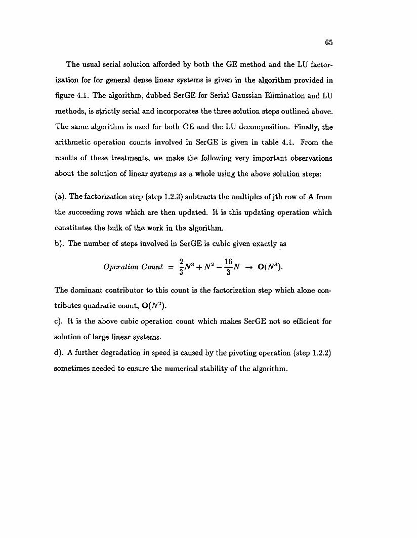
65

The usual serial solution afforded by both the GE method and the LU factor­

ization for for general dense linear systems is given in the algorithm provided in

figure 4.1. The algorithm, dubbed SerGE for Serial Gaussian Elimination and LU

methods, is strictly serial and incorporates the three solution steps outlined above.

The same algorithm is used for both GE and the LU decomposition. Finally, the

arithmetic operation counts involved in SerGE is given in table 4.1. From the

results of these treatments, we make the following very important observations

about the solution of linear systems as a whole using the above solution steps:

(a). The factorization step (step 1.2.3) subtracts the multiples of jth row of A from

the succeeding rows which are then updated. It is this updating operation which

constitutes the bulk of the work in the algorithm.

b). The number of steps involved in SerGE is cubic given exactly as

Operation Count = ^-N3 + N 2 — -^-N —> 0 ( N 3).o o

The dominant contributor to this count is the factorization step which alone con­

tributes quadratic count, 0 ( N 2).

c). It is the above cubic operation count which makes SerGE not so efficient for

solution of large linear systems.

d). A further degradation in speed is caused by the pivoting operation (step 1.2.2)

sometimes needed to ensure the numerical stability of the algorithm.

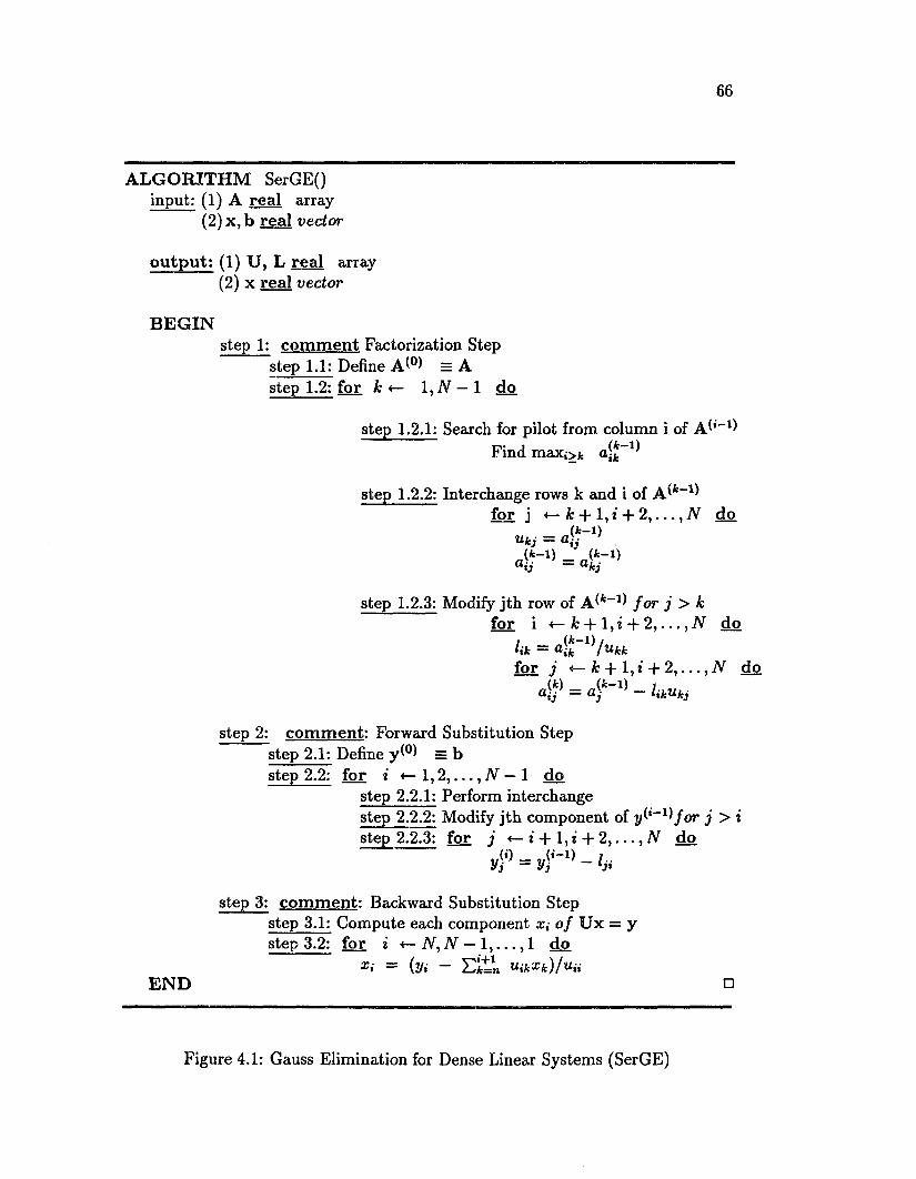
66

A L G O R IT H M SerGE() input: (1) A real array

(2) x, b real vector

o u tp u t: (1) U , L real array (2) x real vector

BEG INstep 1: com m ent Factorization Step

step 1.1: Define A^0 = A step 1.2: for k <— 1 ,N — 1 do

step 1.2.1: Search for pilot from column i of A*'-1) Find maxj>fc a-£-1^

step 1.2.2: Interchange rows k and i of A ^ -1)for j +— k + l , t + 2 , . . . , N do

( t - i )

®ij kj

step 1.2.3: Modify jth row of A ^ -1 fo r j > kfor i <— k + l , i + 2 , . . . , N do

l ik = a!fe_1)/«fcfcfor j <— k + 1, i + 2 , . . . , N do

a«i) = ajfc_1) ~ ^ U k j

step 2: com m ent: Forward Substitution Stepstep 2.1: Define y(°) = b step 2 .2 : for i +— 1, 2 , 1 do

step 2.2.1: Perform interchangestep 2.2.2: Modify jth component of y ^ ' ^ f o r j > istep 2.2.3: for j *— i + l , i -f 2 , . . . , N do

V] Vj

step 3: com m en t: Backward Substitution Stepstep 3.1: Compute each component r t- o f U x = y step 3.2: for i «— N, N — 1, . . . , 1 do

Xi = (yi ~ E li1* u ikx h) / u nE N D □

Figure 4.1: Gauss Elimination for Dense Linear Systems (SerGE)

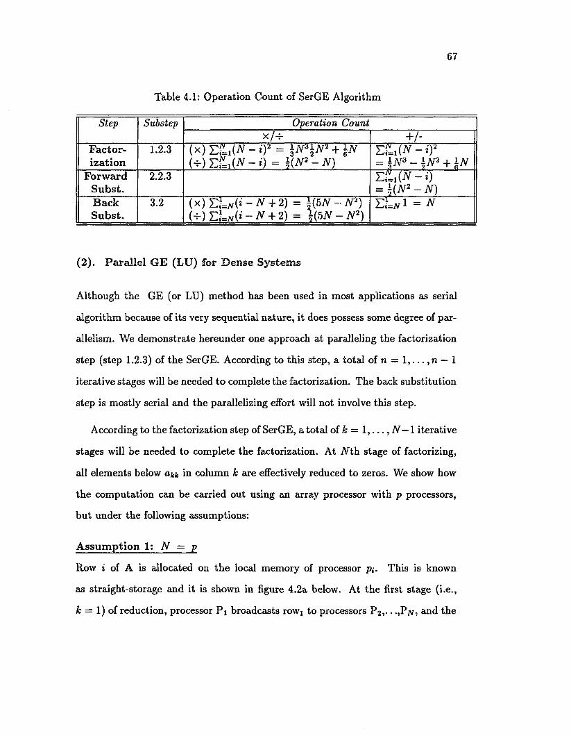
67

Table 4.1: Operation Count of SerGE Algorithm

Step Substep Operation Countx / + + /•

F acto r­ization

1.2.3 (x )E f= ,(A f - i ) i = p V a p P + lAT W E * , ( J » - i ) = i ( N 2 - N ) = 1N 3 - 1N 2 + 1N

Forw ardS ubst.

2.2.3 E L ( N - i) = U N 2 - N)

BackS ubst.

3.2 ( x ) Z U ( i - N + 2) = « 5 N - N 2) M -JV + 2) = « 5 N - N 2)

Z L w 1 = N

(2). P ara lle l G E (LU) for D ense S ystem s

Although the GE (or LU) method has been used in most applications as serial

algorithm because of its very sequential nature, it does possess some degree of par­

allelism. We demonstrate hereunder one approach at paralleling the factorization

step (step 1.2.3) of the SerGE. According to this step, a total of n = 1 , . . . ,n — 1

iterative stages will be needed to complete the factorization. The back substitution

step is mostly serial and the parallelizing effort will not involve this step.

According to the factorization step of SerGE, a total of k = 1 , . . . , N —l iterative

stages will be needed to complete the factorization. At Nt h stage of factorizing,

all elements below a** in column k are effectively reduced to zeros. We show how

the computation can be carried out using an array processor with p processors,

but under the following assumptions:

A ssum ption 1 : N = p

Row i of A is allocated on the local memory of processor p,. This is known

as straight-storage and it is shown in figure 4.2a below. At the first stage (i.e.,

k = 1) of reduction, processor P i broadcasts rowi to processors P2, . . .,Pw, and the

68

computation (see step 1.2.3)

Ul ~ Ctjj = fljj j — 2 , . . . , N (4.9)

axe carried out by processors P 2,. • • >Pn in parallel. At stage k = 1, the process is

repeated during which processor P2 broadcasts row2 to processors P3, . . .,Pn, and

these processors compute

/i2 = Os'2/ a22i aij = a»j l«2a2j) j = 3, . . . , N. (4.10)

This process of reduction process is repeated another n — 2 times to complete

factorization of A into L and U. In actual implementation, L and U overwrite the

original matrix A.

Although this process is easy to implement on any array processor, it, however,

has 2 major drawbacks:

1). There is a considerable data communication at each stage.

2). The number of active processors decrease by one at a completion of each stage.

The problem of existence of idle processors is known as load balance problem, and

it is a serious drawback that, with judicious design of data structures, should be

minimized if not altogether eliminated.

A ssum ption 2 : JV > p

Load balance difficulty may be mitigated by making judicious storage of A. Sup­

pose p> n. Then the storage of the rows of A can be interleaved among the

processors. Assuming that n = kp, rows 1, p + 1, p + 2 ,... are stored on

processor 1, rows 2, p + 2, 2p + 2 , . . . on processor 2, and so on. Again, row 1

will be sent from processor Pi to the other processors and then the computation

of eq.(4.9) and eq.(4.10) will be done in blocks of k sets of operations in each

processor. As before, processors will become idle as the computation proceeds,

but this storage greatly alleviates the problem of processors becoming idle. This

69

A L G O R IT H M ParGE()B E G IN

step 1 : b ro ad cast (row 1) s te p 2 ;

for k <— 1, N — 1 dos tep 2 .1 : i f k $ EOW jj th e n

receive (row k)

2 .2 : forall rows (i > k ) and (ke ROW *) do Uk = 0-ik/o.kk for j *— k + 1, N do

= h i Qik&k}| f (t = k) and (iy£ iV)th en

b roadcast (row 1)EN D

Figure 4.2: Parallel GE and LU Factorization for Dense Linear Systems (ParGE)

type of storage is known as wrapped-interleaved storage [ORTEGA 88]. We now

give an algorithm based upon the wrapped-interleaved storage scheme. We call

the algorithm ParGE for Parallel Gauss Elimination (and LU) method. In this

algorithm, ROW,- is a set of indices of rows of A allocated to a processor P,-.

Thus, for processor P 1} R 0 W i= { l,p + l,2 p + l,.. .,(k-l)p+l}, and for processor P3,

ROW3={3,p+3,2p+3,.. .,(k-l)p+3}, and so on. In the ParGE algorithm, the com­

putation of multipliers are begun while some part of the pivot row is received. For

example, the computation of multipliers hi begin as soon as an is received rather

than waiting for the entire pivot row to be received. This way, the communication

delay is minimized, and the overall load-balance improved.

70

4 .2 .1. 2 G E & LU F acto riza tion for B anded L inear S ystem s

1 . Serial G E (LU) for B anded L inear System s The serial Gauss Elimina­

tion method (SerGE) given above for general dense linear systems is very inefficient

for the solution of large sparse systems because of a potentially large number of

zeros in such systems. The algorithm SerGE handles the matrix A and vector k in

entirety, that is, all the elements of A and of vectors are processed according to the

iterative steps of the algorithm. Since for our model problem A is highly sparse,

SerGE would be very ill-suited indeed for the solution of such a system since a very

large number of zero elements would be processed. Hence, to use SerGE to solve

our model problem, an extensive modification must be in order, and , moreover,

appropriate data structures capable of holding the nonzero elements of A and k

are needed.

Below, we give a modified version of SerGE suitable for solution of block-

tridiagonal linear systems depicted in eq.(4.2). We call the algorithm SerGET

for Serial Gauss Elimination for Tridiagonal linear systems. Although SerGET is

the Gaussian Elimination algorithm for block-tridiagonal systems, the same algo­

rithm is used for LU factorization for tridiagonal systems, with slight modifications

mainly aimed at retaining the resulting matrices U and L. The major distinctive

feature of SerGET algorithm is a set of data structures used to hold mostly the

nonzero elements of matrix A.

In the forward elimination step (step 1), three auxiliary vectors u, /, y are

precomputed at every iteration step. These auxiliaries are functions of A only. In

table 4.2, we give the operation count of the SerGET algorithm. The total number

of iterative steps needed by the algorithm is lOn. The four loops of SerGET in

steps 1.2, 1.4, 1.6, and 2.2 are all sequential recurrences that must be evaluated

one term at a time. This, together with the fact that the vector elements are

71

A L G O R IT H M SerGET() in p u t: (1) a rea l array

(2) k real vector o u tp u t: (1) k real array com m ent: k is overwritten with solution x

(2) a real vector com m ent: holds L & U Locals: (1) u real vector

(2 ) 1 rea l vector(3) y real vector

B E G INste p 1 : com m ent Forw ard E lim ination S tep

s tep 1 .1 : ui <— ki s te p 1 .2 : for i *— 2 , N — 1 do

Ui «- ki - (a,Ci_i/m - i)

s te p 1.3: li *— a2/&i s tep 1.4: fo r i *— 2, N do

U <- a»/«,-i

s tep 1.5: yi *— k\ s tep 1 .6 : fo r i *— 2, N do

yi ki - hyi-i

s tep 2 : com m ent Back E lim ination S teps te p 2 .1 : x„ ♦- yn/u n s te p 2 .2 : for i *— n — 1,1 do

♦- (Vi ~ Xi+iCi/uiE N D

Figure 4.3: Gauss Elimination for Tridiagonal Systems (SerGET)

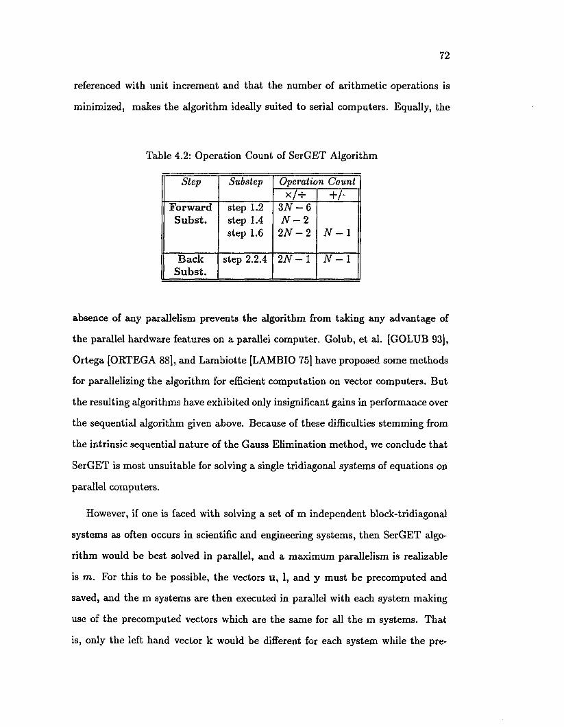
72

referenced with unit increment and that the number of arithmetic operations is

minimized, makes the algorithm ideally suited to serial computers. Equally, the

Table 4.2: Operation Count of SerGET Algorithm

Step Substep Operation CountX/-S- + /•

Forw ardS ubst.

step 1.2 step 1.4 step 1.6

31V — 6 N - 2

2 N - 2 N - 1

BackS ubst.

step 2.2.4 2 N - 1 IV - 1

absence of any parallelism prevents the algorithm from taking any advantage of

the parallel hardware features on a parallel computer. Golub, et al. [GOLUB 93],

Ortega [ORTEGA 88], and Lambiotte [LAMBIO 75] have proposed some methods

for parallelizing the algorithm for efficient computation on vector computers. But

the resulting algorithms have exhibited only insignificant gains in performance over

the sequential algorithm given above. Because of these difficulties stemming from

the intrinsic sequential nature of the Gauss Elimination method, we conclude that

SerGET is most unsuitable for solving a single tridiagonal systems of equations on

parallel computers.

However, if one is faced with solving a set of m independent block-tridiagonal

systems as often occurs in scientific and engineering systems, then SerGET algo­

rithm would be best solved in parallel, and a maximum parallelism is realizable

is m. For this to be possible, the vectors u, 1, and y must be precomputed and

saved, and the m systems are then executed in parallel with each system making

use of the precomputed vectors which are the same for all the m systems. That

is, only the left hand vector k would be different for each system while the pre-

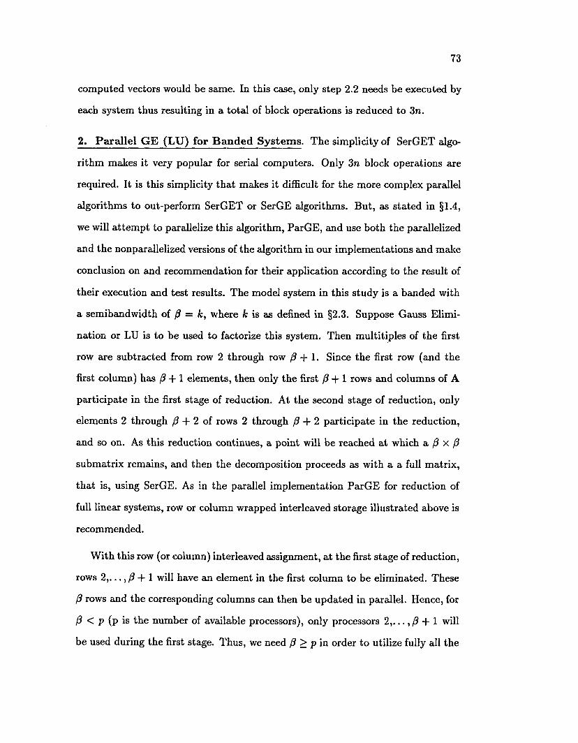
73

computed vectors would be same. In this case, only step 2.2 needs be executed by

each system thus resulting in a total of block operations is reduced to 3n.

2. P ara lle l G E (LU) for B anded S ystem s. The simplicity of SerGET algo­

rithm makes it very popular for serial computers. Only 3n block operations are

required. It is this simplicity that makes it difficult for the more complex parallel

algorithms to out-perform SerGET or SerGE algorithms. But, as stated in §1.4,

we will attem pt to parallelize this algorithm, ParGE, and use both the parallelized

and the nonparallelized versions of the algorithm in our implementations and make

conclusion on and recommendation for their application according to the result of

their execution and test results. The model system in this study is a banded with

a semibandwidth of /? = fc, where & is as defined in §2.3. Suppose Gauss Elimi­

nation or LU is to be used to factorize this system. Then multitiples of the first

row are subtracted from row 2 through row /? + 1. Since the first row (and the

first column) has (3 + 1 elements, then only the first (3 + 1 rows and columns of A

participate in the first stage of reduction. At the second stage of reduction, only

elements 2 through (3 -j- 2 of rows 2 through (3 + 2 participate in the reduction,

and so on. As this reduction continues, a point will be reached at which a (3 x (3

submatrix remains, and then the decomposition proceeds as with a a full matrix,

that is, using SerGE. As in the parallel implementation ParGE for reduction of

full linear systems, row or column wrapped interleaved storage illustrated above is

recommended.

With this row (or column) interleaved assignment, at the first stage of reduction,

rows 2 ,. . . , f3 + \ will have an element in the first column to be eliminated. These

f3 rows and the corresponding columns can then be updated in parallel. Hence, for

(3 < p (p is the number of available processors), only processors 2 ,...,/? + 1 will

be used during the first stage. Thus, we need (3 > p in order to utilize fully all the

74

processors. We conclude this discussion with a few words of caution: The method

of parallelizing LU reduction is

a) recommended for a banded systems with large /?, especially those with 0 > p

b) completely inadequate if the system has 0 = 1 , that is, a tridiagonal system. In

this case the final submatrix, being ( 3 x / ? = l x l , would contain a single element,

c) more prone to load-imbalance even if 0 > p.

Because the parallel solution of banded system whose 0 = 1 is trivial, we will

not try to parallelize the GE or LU methods when our system is cast in block

tridiagonal form. That is, we will endeavor to parallelize only the original model

system with 0 = k.

3. R e la tin g G E & LU IN T h e S erG E T A lg o rith m . Before leaving SerGET

algorithm for the moment, we want to emphasize the fact that the auxiliary vectors

u and 1 are the coefficients in the triangular decomposition of A into the product

of a triangular matrix L and an upper triangular matrix U:

A x = LU,

where

L =

and where

( 1 0 I2 1 0

0 \

In - 1 1 0 0 0 lN 1 )

(4.11)

75

U =

ui Ci 00 «2 C2

0

0

0 0In - i c n - i

UN /

(4.12)

The reader may have noted that in the above LU factorization, we have used the

Croute’s approach among the three most populax factorization methods character­

ized with the following properties:

Croute : la = 1

Doolittle : ua = 1

Choleski :

Vi, 1 < * < N.

4.2.2 Orthogonal Factorization for Banded System s

An alternative to the LU decomposition is the factorization

A P = Q R (4.13)

Here A is any mXn matrix, not just square matrix or, as in the case of Choleski

factorization scheme a symmetric positive definite matrix, P is an nXn permu­

tation matrix,Q an mXm orthogonal matrix, and R an mXn upper triangular

matrix. There axe a number of approaches to obtaining the factorization indicated

in eq. (4.2.2). These usually differ in the way the permutation matrix P is derived

and on the nature of the system. Two commonest such factorization approaches

are the Householder and the Givens factorization schemes.

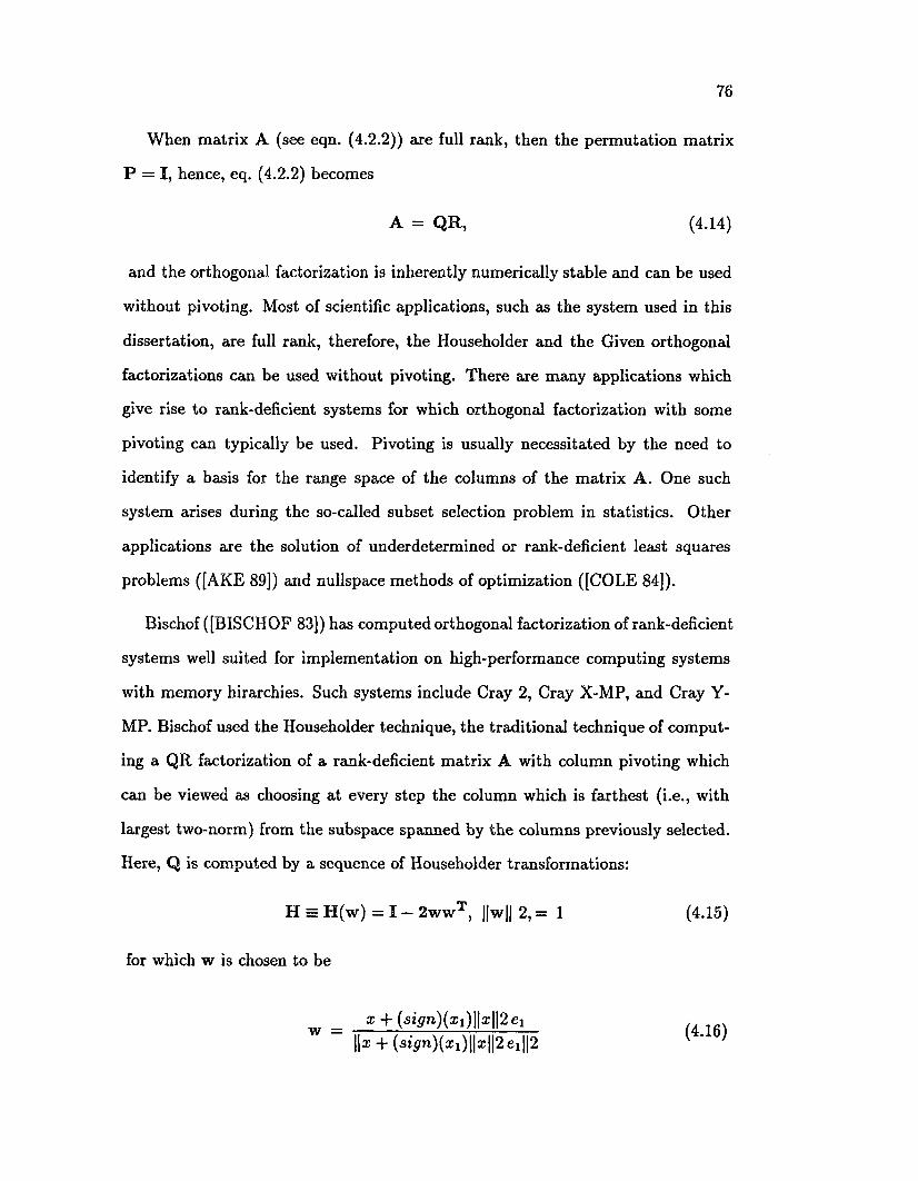
76

When matrix A (see eqn. (4.2.2)) are full rank, then the permutation matrix

P = I, hence, eq. (4.2.2) becomes

A = Q R, (4.14)

and the orthogonal factorization is inherently numerically stable and can be used

without pivoting. Most of scientific applications, such as the system used in this

dissertation, are full rank, therefore, the Householder and the Given orthogonal

factorizations can be used without pivoting. There are many applications which

give rise to rank-deficient systems for which orthogonal factorization with some

pivoting can typically be used. Pivoting is usually necessitated by the need to

identify a basis for the range space of the columns of the matrix A. One such

system arises during the so-called subset selection problem in statistics. Other

applications are the solution of underdetermined or rank-deficient least squares

problems ([AKE 89]) and nullspace methods of optimization ([COLE 84]).

Bischof ([BISCHOF 83]) has computed orthogonal factorization of rank-deficient

systems well suited for implementation on high-performance computing systems

with memory hirarchies. Such systems include Cray 2, Cray X-MP, and Cray Y-

MP. Bischof used the Householder technique, the traditional technique of comput­

ing a QR factorization of a rank-deficient matrix A with column pivoting which

can be viewed as choosing at every step the column which is farthest (i.e., with

largest two-norm) from the subspace spanned by the columns previously selected.

Here, Q is computed by a sequence of Householder transformations:

H = H (w ) = I — 2wwT, ||w|| 2, = 1 (4.15)

for which w is chosen to be

||x + (sipn)(x1)||a:||2 ex||2

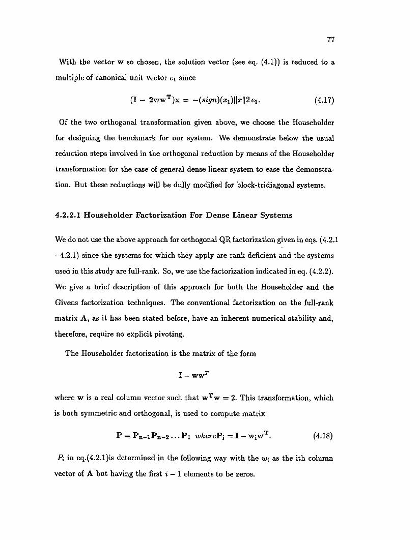
77

With the vector w so chosen, the solution vector (see eq. (4.1)) is reduced to a

multiple of canonical unit vector ex since

(I — 2 w w t ) x = -{sign)(xi)\\x\\2ei. (4-17)

Of the two orthogonal transformation given above, we choose the Householder

for designing the benchmark for our system. We demonstrate below the usual

reduction steps involved in the orthogonal reduction by means of the Householder

transformation for the case of general dense linear system to ease the demonstra­

tion. But these reductions will be dully modified for block-tridiagonal systems.

4.2.2.1 Householder Factorization For D ense Linear System s

We do not use the above approach for orthogonal QR factorization given in eqs. (4.2.1

- 4.2.1) since the systems for which they apply are rank-deficient and the systems

used in this study are full-rank. So, we use the factorization indicated in eq. (4.2.2).

We give a brief description of this approach for both the Householder and the

Givens factorization techniques. The conventional factorization on the full-rank

matrix A, as it has been stated before, have an inherent numerical stability and,

therefore, require no explicit pivoting.

The Householder factorization is the matrix of the form

I — wwr

where w is a real column vector such that w Tw = 2. This transformation, which

is both symmetric and orthogonal, is used to compute matrix

P = P n - lP n - 2 • • • P i wherePi = I — wjw1 . (4-18)

Pi in eq.(4.2.1)is determined in the following way with the u;; as the ith column

vector of A but having the first i — 1 elements to be zeros.

78

Let aj be the ith column vector of A. Also, let

uT = (an - s, a2h. . . , ani), wj = /zu, (4.19)

where

u T = 7 = (s2 - a,-,s)_1, fi = 7 2 , (4.20)

and the sign of s is chosen to be opposite that of a,-,- for numerical stability. Then

WiTwi = n2((an - s f + £ 4 ) = fi(s2 - a{is) = -i=2 ^

so that

T v ( a u - 3)a n — WjW: aj = a „ 1------------- = 3

Mrp CL 2 i IX

aji — WjWi ai = a j i — = 0 j = * + 1 ,i + 2 , . . . , N

which shows that the subdiagonal elements on column i of A have been reduced

to zeros. At the ith step of this reduction, P,- is determined to be P,- = I — w i w j .

The Householder algorithm computes the matrices P,- for i = 1 ,2 ,. . . n — 1 using

the column vectors wj as defined above. The Pj so determined are used to compute

matrix P according to eq.(4.2.1). With P , R and Q of eq.(4.2.2) axe determined

with

PA = P n -lP n -2 • • • P i A = R (4.21)

and Q = P -1 (4.22)

where R is upper triangular, and the matrices P,- are all orthogonal so that P =

P „ _ i . . . P i and P _1 are also orthogonal matrics. The bulk of the work in carrying

out the Householder reduction to triangulax form is updating the nonzero columns

of A at each stage. The Householder transformation for linear dense systems is

given in Figure 4.4.

79

A L G O R IT H M HouseHolderQ in p u t: a real array o u tp u t: a real array Local: (1) u real vector

(2) s real vector(3) a real vector(4) 7 rea l vector

B E G INstep 1.: for k «— 1,1V — 1 do

step 1 .1 : sjb < sgn(ctkk) (£JL* afk)* , 7* = (s* - a****)"1s tep 1 ,2 : 11 ♦ (0 , . . . , 0 , ctkk ~~~ ? &nk)s tep 1.3: afefc *— s*s tep 1.4: for j <— k + l , N do

s tep 1.4.1: atj <— (7*u£)aj s tep 1.4.2: a,- aj — alpha^-u^

E N D □

Figure 4.4: Householder Reduction for Dense Linear Systems

4.2 .2 .2 H ouseholder F acto riza tion For B anded L inear S ystem s

We consider the Orthogonal reduction of a banded linear system having a semiband­

width of /?. The reduction, like in the case of LU reduction, also expands the band-

widths above the main diagonal. When the Householder transformation I — ww T

is applied to matrix A in order to zero elements of the first column below the main

diagonal, then w is of the form wT — ( * , . . . , o, . . . , 0) in which the first ft + 1

elements are, in general, nonzero. Then the new ith column of A is a; — w Tajw,

where a; is the ith column of A. The first Householder transformation introduces,

in general, nonzero elements outside the original band. No further nonzero ele­

ments are introduced since, on the first transformation, w Taj = 0 for i > 2ft + 1.

On the second Householder transformation, nonzeros will be introduced into 2ft+ 2

column, starting in the second element. At each subsequent transformation, nonze-

80

ros will be introduced in one more column so that at the end of the triangular

reduction, the upper triangular matrix will have a bandwidth of 2/3 + 1.

4.3 ITERATIVE BENCH M ARK S

Iterative methods are commonly used to solve large, sparse systems of linear equa­

tion for three major reasons:

1. Iterative methods require a minimum of storage, usually on the same order

as the number of nonzero entries of the matrix A (see eq.(4.1)), whereas a

direct methods (e.g., Gauss Elimination) usually cause fill-in of A as their

computation with A proceeds, and, therefore, the advantages of sparcity of

A are usually partly lost.

2. Generally, iterative methods lend themselves to easy parallelizing than do

direct methods. We learned this during the parallelizing attempts of some

direct methods in §4.1. Many iterative methods (e.g., Jacobi) have inherent

parallel features which are usually obvious and easy to exploit, although such

exploitation could be limited by less-than-satisfactory convergence rates.

3. Iterative methods reduce the amount of actual computation needed to solve

linear system of equations. This is especially true for our model problem if

cast in three dimensions.

Iterative methods, however, have some disadvantages over direct methods.

1. Iterative methods require initial guess of the solution vector x (see eq.(4.1)).

Direct methods, on the other hand, at least theoretically, do not involve

iteration and, therefore, do not require initial guesses of solution.

81

2. The rate of convergence of iterative methods are dependent on the quality

of the initial guess of the solution vector, whereas, direct methods, because

they do not require initial guesses of solution, theoretically should give exact

solution. Of course, this is seldom the case chiefly because of limitations

imposed by round-off, and other computation-related errors.

3. The convergence rates of iterative methods are generally poorer (e.g., Jacobi)

than those of direct methods, and these rates are almost always improved

with some mathematical means (e.g., relaxation techniques), and by refor-

mating the methods accordingly.

In this section, we intend to develop some parallel algorithms based on some

iterative methods and then use such algorithms as benchmarks for testing the new

algorithm for parallel solution of the model problem. The iterative approaches

that are used are the symmetric over-relaxation method or SOR, and the conjugate

gradient method. We will follow the approach of algorithmic development adopted

in §4.1 — a brief overview of the essential steps embodied in the formulation of the

chosen method when applied for solving dense linear systems, and then parallelizing

the method mainly along those steps for the solution of the model problem on a

parallel processor.

4.3.1 Sym m etric Over-relaxation M ethod (SOR)

4.3.1.1 T h e SO R M eth o d For D ense L inear S ystem s

Assume that the linear system depicted in eq.(4.1) is dense, that an IV x N matrix

A is nonsingular, and that x and k are n-dimensional vectors. Let D be diagonal

matrix of A, and Z = I — D -1 A. Then eq.(4.1) can be rewritten as

D _1A x = D -1k

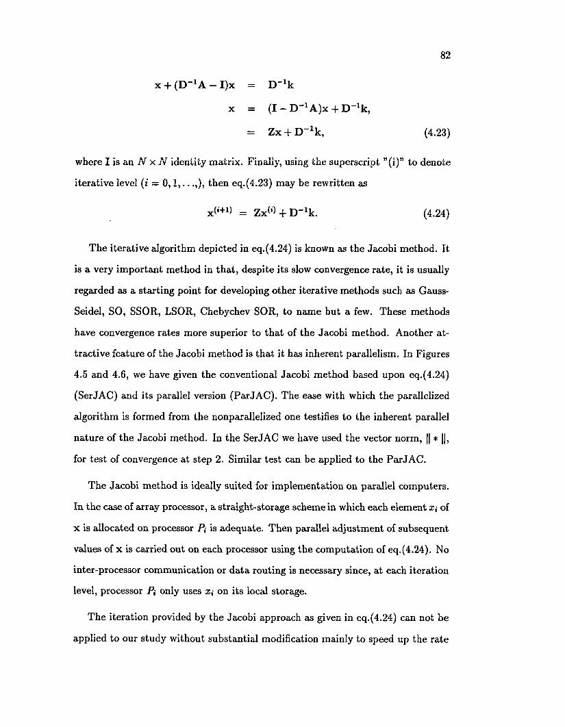
82

x + ( D '1 A - I)x = D _1k

x = (I — D _1 A )x + D -1k,

= Zx -f D -1k, (4.23)

where I is an N x N identity matrix. Finally, using the superscript ”(i)” to denote

iterative level (i = 0 ,1 ,...,) , then eq.(4.23) may be rewritten as

x<*'+1) = Zx(,) + D _1k. (4.24)

The iterative algorithm depicted in eq.(4.24) is known as the Jacobi method. It

is a very important method in that, despite its slow convergence rate, it is usually

regarded as a starting point for developing other iterative methods such as Gauss-

Seidel, SO, SSOR, LSOR, Chebychev SOR, to name but a few. These methods

have convergence rates more superior to that of the Jacobi method. Another a t­

tractive feature of the Jacobi method is that it has inherent parallelism. In Figures

4.5 and 4.6, we have given the conventional Jacobi method based upon eq.(4.24)

(SerJAC) and its parallel version (ParJAC). The ease with which the parallelized

algorithm is formed from the nonparallelized one testifies to the inherent parallel

nature of the Jacobi method. In the SerJAC we have used the vector norm, || * ||,

for test of convergence at step 2. Similar test can be applied to the ParJAC.

The Jacobi method is ideally suited for implementation on parallel computers.

In the case of array processor, a straight-storage scheme in which each element x,- of

x is allocated on processor P, is adequate. Then parallel adjustment of subsequent

values of x is carried out on each processor using the computation of eq.(4.24). No

inter-processor communication or data routing is necessary since, at each iteration

level, processor P; only uses x,- on its local storage.

The iteration provided by the Jacobi approach as given in eq.(4.24) can not be

applied to our study without substantial modification mainly to speed up the rate

83

A L G O R IT H M SerJACQ in p u t: (1) A rea l array

(2) x ,k real vector(3) e real scalar

com m ent: e used to stop iter.

o u tp u t: x real vectorcom m ent: x is Guessed: x =(xq° \ x i ° \ . . . , x ^ j )

B E G INstep 1: Precompute matrices the D &c Zs te p 2: for i <— 1. fo rever n do

xW = . Z x ^ + D ^ kIf ||x* - X * - 1 (I < £ th e n

r e tu rn fx ^ )E N D □

Figure 4.5: Serial Jacobi Method for Dense Linear Systems (SerJAC)

A L G O R IT H M ParJACQ B E G IN

step 1: Precompute matrices the D & Z s tep 2: Allocate x = (x0, . . . , xn_j) such that x,- is on local

memory of processor Pi s tep 3: forall (Pi) do

xW = Z x ^ + D ^ k E N D □

Figure 4.6: Parallel Jacobi Method for Dense Linear Systems (ParJAC)

84

of convergence. Unfortunately, as we will see shortly, speeding up convergence rate

comes with a severe price — the loss of obvious parallelism in the original Jacobi

method.

The fact that Jacobi method, or any method for that matter, can be efficiently

implemented on parallel computers does not necessarily mean that it is a good

method to use because one must also consider the number of iterations that are

required to obtain a satisfactory convergence. The Jacobi method, becuse of its

slow convergence rate, must be modified so that it cam achieve a better rate of

convergence.

The modification is usually achieved by combining the Jacobi method with

the Gauss-Seidel approach. The gauss Seidel method performs iteration as given

in eqs.(4.23, 4.24) above but with one important difference: in the computation

of xb+1) from x^), computer values for x^,+1) are substituted for values in x ^

as soon as they are available during the course of computation. In other words,

the computation of x^,+1) commences as soon as x ^ becomes available at the

same iteration level, whereas in Jacobi or JOR, iteration at a level commences

after cessation of iterations at previous level. The Gauss-Seidel method involves

computing x^‘+1\ and immediately setting x ^ *— x(,+1).

The combination of the Gauss-Seidel method and overrelaxation method is

called succesive overrelaxation method or SOR. Experience and theoretical results

show that SOR, most of the times, converges faster than Jacobi and JOR methods.

SOR amounts to using the computation:

x<’+1> = + (1 — wL)_1wDk (4.25)

where D is the diagonal matrix of A, Z as defined before (see eq.(4.24)), U , L are

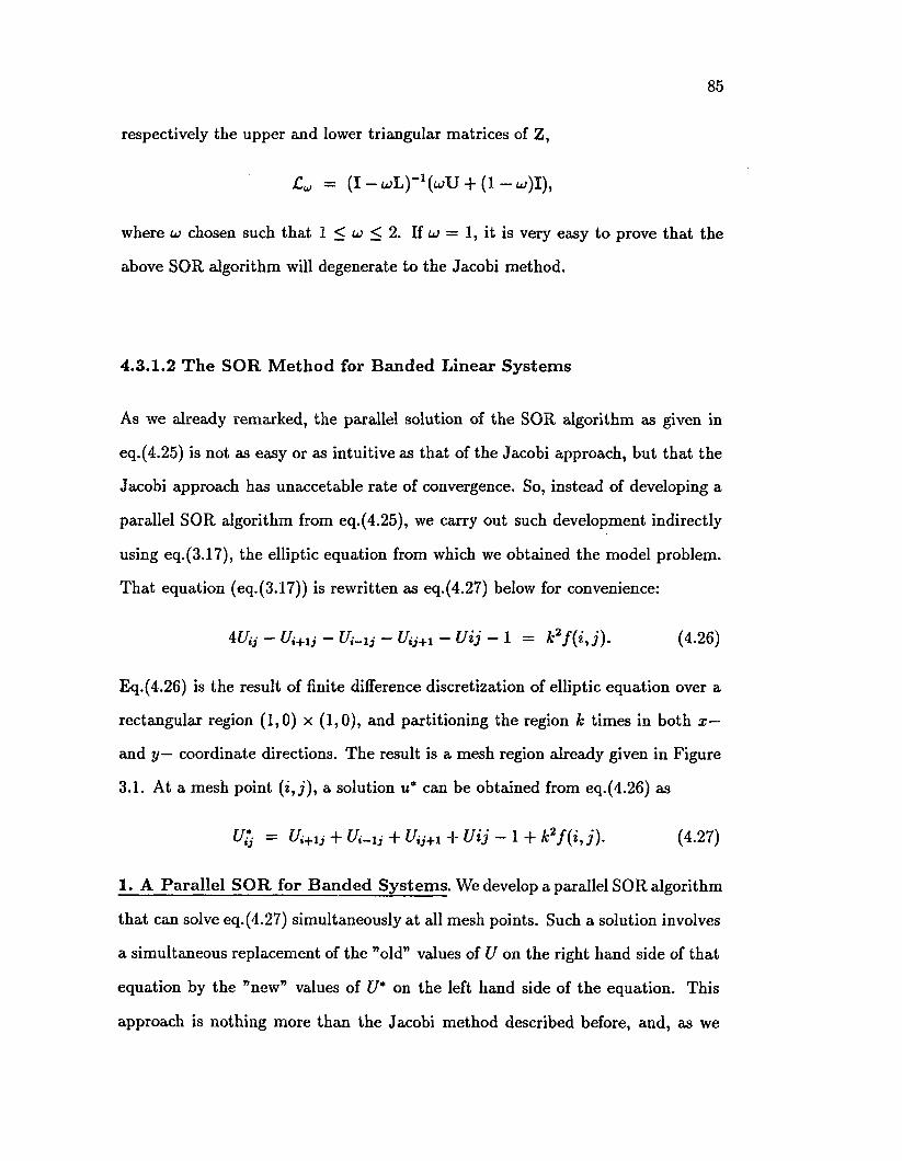
85

respectively the upper and lower triangular matrices of Z,

Cu = ( I - u ^ - V U + t l - a ; ) ! ) ,

where u chosen such that 1 < u < 2. If uj = 1, it is very easy to prove that the

above SOR algorithm will degenerate to the Jacobi method.

4.3.1.2 The SOR M ethod for Banded Linear System s

As we already remarked, the parallel solution of the SOR algorithm as given in

eq.(4.25) is not as easy or as intuitive as that of the Jacobi approach, but that the

Jacobi approach has unaccetable rate of convergence. So, instead of developing a

parallel SOR algorithm from eq.(4.25), we carry out such development indirectly

using eq.(3.17), the elliptic equation from which we obtained the model problem.

That equation (eq.(3.17)) is rewritten as eq.(4.27) below for convenience:

4Uij - Ui+lj - - Uij+1 - Uij - 1 = k2f ( i , j ) . (4.26)

Eq.(4.26) is the result of finite difference discretization of elliptic equation over a

rectangular region (1,0) x (1,0), and partitioning the region k times in both x —

and y — coordinate directions. The result is a mesh region already given in Figure

3.1. At a mesh point a solution u* can be obtained from eq.(4.26) as

U*j = Ui+ij + Ui-ij + Uij+i -f- Uij — 1 + k2f ( i , j ) . (4.27)

1. A P ara lle l SO R for B anded S ystem s. We develop a parallel SOR algorithm

that can solve eq.(4.27) simultaneously at all mesh points. Such a solution involves

a simultaneous replacement of the ”old” values of U on the right hand side of that

equation by the ”new” values of U* on the left hand side of the equation. This

approach is nothing more than the Jacobi method described before, and, as we

86

observed then, such a simultaneous replacement is ideally suited for implementa­

tion on parallel computers. Simultaneous adjustment means that eq.(4.27) can be

evaluated at all mesh points in parallel with the maximum parallelism of n2. In

Typical scientific and engineering applications, N = 32 to 256, so that parallelism

varies from about 1000 to about 64,000. This leads to satisfactorily long vectors

for efficient implementation on pipelined computers. On the other hand, for ar­

ray processor such as MasPar MP-X, the mesh can probably be chosen to fit the

machine size or multiples of it. Since each mesh point needs values of U from at

most 4 neighbors, a nearest-neighbor communication, the obvious communication

primitive to use for inter-processor communication and data routings are the Xnet

or Xnetc available in MPL of the MP-X.

Because of the slow convergence rate, the above Jacobi algorithm for simulta­

neous adjustment of u at all mesh points will not be used. Instead we use the

SOR method, which, by direct algebraic manipulation of the SOR equation given

in eq.(4.24), gives in the present case the following solution which is equivalent to

eq.(4.27):

U%*° = + (1 - u>)U?Jd, (4.28)

where, as before, a; is a constant relaxation factor used improve the convergence

rate and chosen such that 1 < u < 2. The SOR equation given in eq.(4.28) de­

generates to the Jacobi equation of eq.(4.27) when u> = 1. For our model problem,

the best convergence rate is obtained with

w = Ub = t .' V i2 ' 2^ ’ (4,29)1 + (1 - p2)2

where A = u>b — 1, and p is the convergence factor corresponding to the Jacobi

iteration. Therefore, p — cos(ir/N) for the model problem.

The results of direct application of eq.(4.28) for simultaneous adjustment of u at

mesh points as found in this study is less than satisfactory, in terms of convergence

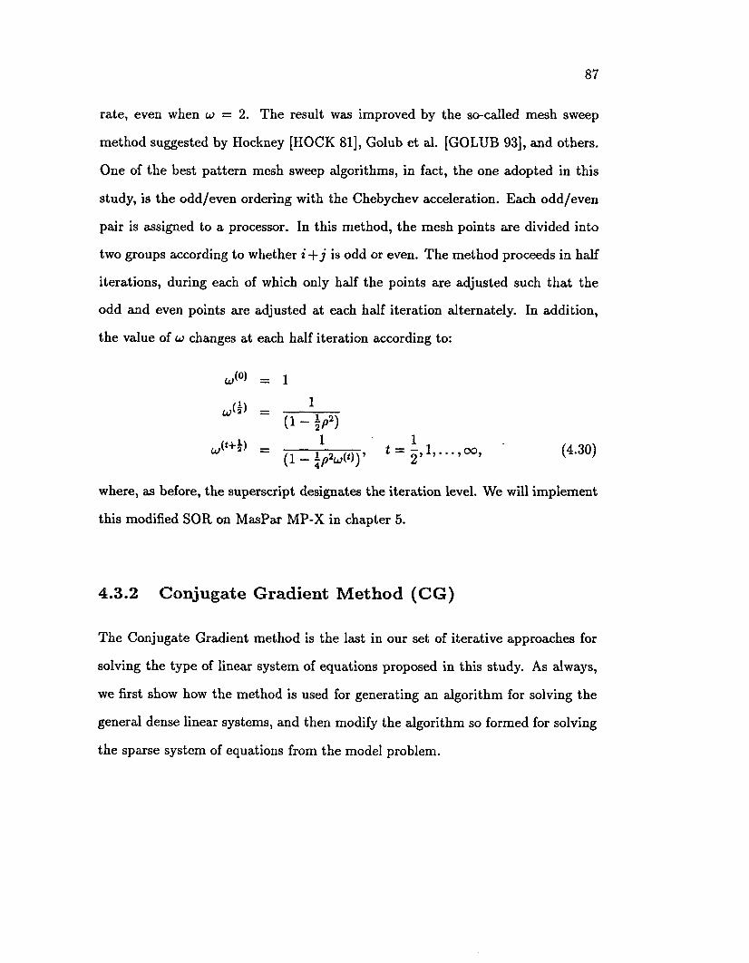
87

rate, even when u = 2. The result was improved by the so-called mesh sweep

method suggested by Hockney [HOCK 81], Golub et al. [GOLUB 93], and others.

One of the best pattern mesh sweep algorithms, in fact, the one adopted in this

study, is the odd/even ordering with the Chebychev acceleration. Each odd/even

pair is assigned to a processor. In this method, the mesh points are divided into

two groups according to whether i + j is odd or even. The method proceeds in half

iterations, during each of which only half the points are adjusted such that the

odd and even points axe adjusted at each half iteration alternately. In addition,

the value of u> changes at each half iteration according to:

u /° > =

=

W(t+a) =

where, as before, the superscript designates the iteration level. We will implement

this modified SOR on MasPar MP-X in chapter 5.

4.3.2 Conjugate Gradient M ethod (CG)

The Conjugate Gradient method is the last in our set of iterative approaches for

solving the type of linear system of equations proposed in this study. As always,

we first show how the method is used for generating an algorithm for solving the

general dense linear systems, and then modify the algorithm so formed for solving

the sparse system of equations from the model problem.

(1 - \P2)

(i -

(4.30)

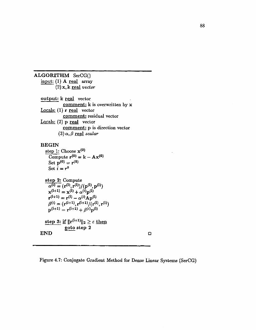
88

A L G O R IT H M SerCG() input: (1) A real array

(2) x, k real vector

output: k real vectorcom m ent: k is overwritten by x

Locals: (1) r real vectorcom m ent: residual vector

Locals: (2) p real vectorcom m ent: p is direction vector

(3) a , 13 real scalar

B E G IN step 1: Choose x^0^

Compute r^0) = k — Ax^°)Set p(°) = r<°>Set i — r°

s te p 2: Compute aW = ( r ^ , r^ )/(pW , pW) x (i+1) = xW + a Wp(i) r (i+i) _ r (i) _ aWApW 0(0 _ (r (i+i)^ r (l+i)/(r (*), r (l)) p(i+i) = P(i+i) + ^(i)p(l) ’

step 3: if ||r(,+ 1 ) | |2 > £ then goto step 2

E N D □

Figure 4.7: Conjugate Gradient Method for Dense Linear Systems (SerCG)

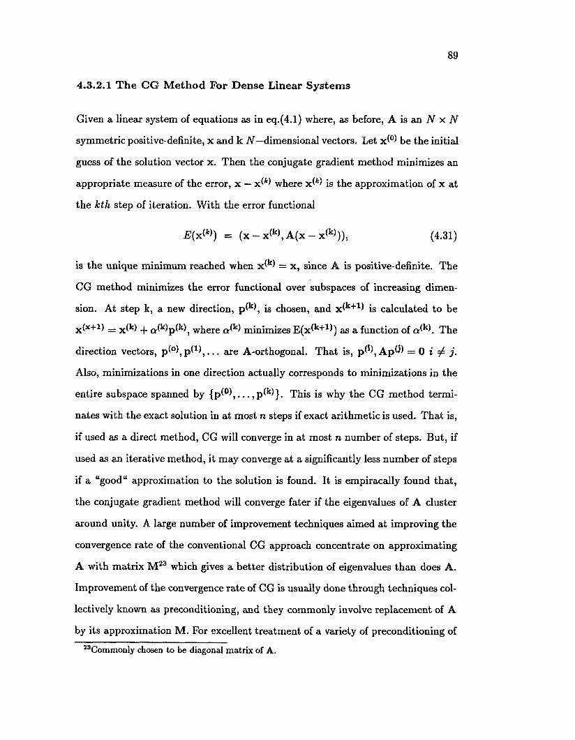
89

4.3.2.1 The CG M ethod For D ense Linear System s

Given a linear system of equations as in eq.(4.1) where, as before, A is an N x N

symmetric positive-definite, x and k A —dimensional vectors. Let x ^ be the initial

guess of the solution vector x. Then the conjugate gradient method minimizes an

appropriate measure of the error, x — x ^ where x ^ is the approximation of x at

the kth step of iteration. With the error functional

E (x& ) = ( x -x < kU ( x - x ( k>)), (4.31)

is the unique minimum reached when x ^ = x, since A is positive-definite. The

CG method minimizes the error functional over subspaces of increasing dimen­

sion. At step k, a new direction, p(k\ is chosen, and x (k+1l is calculated to be

X(x+1) = x (k) -f a(k)p(k), where minimizes E(x^k+1l) as a function of or^l. The

direction vectors, p(°), p i1) , . . . are A-orthogonal. That is, p(*\ Ap(j) = 0 i ^ j.

Also, minimizations in one direction actually corresponds to minimizations in the

entire subspace spanned by { p (° \ . . . , p ^ } . This is why the CG method termi­

nates with the exact solution in at most n steps if exact arithmetic is used. That is,

if used as a direct method, CG will converge in at most n number of steps. But, if

used as an iterative method, it may converge at a significantly less number of steps

if a “good“ approximation to the solution is found. It is empiracally found that,

the conjugate gradient method will converge fater if the eigenvalues of A cluster

around unity. A large number of improvement techniques aimed at improving the

convergence rate of the conventional CG approach concentrate on approximating

A with matrix M 23 which gives a better distribution of eigenvalues than does A.

Improvement of the convergence rate of CG is usually done through techniques col­

lectively known as preconditioning, and they commonly involve replacement of A

by its approximation M. For excellent treatment of a variety of preconditioning of

23Commonly chosen to be diagonal matrix of A.

90

CG, see the work of Baucom [BAUCOM 88]. Figure 4.7 is an algorithm, SerCG,

for solving a dense linear system based upon the above described formulations.

Note that the function (x ,y ) is inner product. That is, (x ,y ) = x Ty. Also, note

that r is residual. Note also that we have used the vector norm for the convergence

test at step 3 following the suggestion by Ortega [ORTEGA 88]. Vector norm has

the advantage of requiring virtually no extra work since (r^+1,r^i+1 ) (of step 3)

will be needed at step 2 of the next iteration level if convergence has not already

occured.

The above conjugate gradient algorithm for dense linear systems is easily extended

to solve in parallel banded systems such as used in this study. On an array proces­

sor such as MP-X, components of vectors such as x ,p ,r are assigned to individual

processors and the vector operations performend on these processors. The multi­

plication of Ap(') follows the treatment of Section 4.2.

4.4 THE NEW TECHNIQUE

We dedicate this section for development of the new algorithm that we believe

is efficient enough to satisfactorily execute the model problem. At the core of

this algorithm design are two powerful direct methods — cyclic reduction and

recursive doubling techniques. There is nothing new about the use of either of the

two methods but their use in combination to construct an algorithm for efficient

solution linear systems is the uniqueness of their application. Cyclic reduction

was developed by Hockney who also was the first to use it to solve tridiagonal

equations on the IBM 7090, a serial processor [HOCK 65]. This method was

chosen in lieu of the Gaussian Elimination technique because it deals with periodic

boundary conditions in a neater fashion than does the elimitation method. For

example, cyclic reduction eliminates computing of auxiliary data structures (see

91

§4.1.1 A) necessitated by the elimination technique. Since its first application by

Hockney, this method, either in its original form or in one or more of its many

modified vesions, has been extensively used by a large number of investigators

to solve various sparse systems ([SWEET 73, SWEET 74, TEMP 80, SWARZ 89,

GOLUB 93]).

Recursive doubling method, proposed by Stone [STONE 73] is a very efficient

technique for parallelizing recursive sequential algorithms. In §4.1.1A, we demon­

strated the difficulties that accompany any attem pt to parallelize the GE and the

LU factorization methods, and stated that these methods are very efficient to use

on serial processors because of their inherent serial nature, and that any advantage

that comes as a result of use of parallelized forms are miniscule, and, as a result,

these methods, are more often than not, used in their serial forms. One major

difficulty in parallelizing these codes is the fact of existence of recurrences in their

mathematical forms given in steps 1.2, 1.6 and 2.2 which are respectively the the

forward elimination and the back substitution of the SerGET algorithm in figure

4.4. For convenience, we rewrite these equations below:

ui = ki

Ui = ki - (a,c,_i/u,_i), 2 < i < N — 1 (4.32)

I2 = a2/fci

/,• = fli/u,--!, 2 < i < N (4.33)

2/i = fci

Vi = h - U v i- i , 2 < i < N (4.34)

= 2In / un

x i = (2li •c i + l c i ) / l t * (4.35)

The forward elimination step is represented by eqs.(4.32, 4.33, and 4.34), while

92

eq.(4.35) determines the back substitution step. Obviously, there are recursions

in eqs.(4.32, 4.33, 4.34) of the forward elimination step, and in eq.(4.35) of the

back elimination step. Eq.(4.32) is said to be nonlinear-recursive because of the

occurence of the nonlinearity, t t ^ , while eqs.(4.33, 4.34, and 4.35) are said to be

linear-recursive.

The presence of any type of recursion in an equation renders an algorithm that

simulates the execution of that equation to be strictly serial for a very obvious rea­

son. Consider a general linear-recursive equation in which x ,a ,d aren-dimensional

vectors:

Xi = di

Xi = a,*,-! + di, 2 < i < N (4.36)

The value of the solution vector x at i = 1 is simply the value of d\ . But the vlaue

of Xj (2 < j < N) depends on the value of Xj- \ , the value computed in the previous

step. Thus, for Xj to be evaluated, Xj-i must first be computed. This algorithm

is strictly serial, simple and elegant and can most be efficiently carried out on a

serial machine. Parallelizing it often results in more complicated and, possibly, less

efficient code. Recursive doubling method affords a very neat introduction into a

recursion.

In this section, both the recursive doubling algorithm and the cyclic reduc­

tion technique are given. Then these are followed by a discussion of how these

approaches are combined to solve our model problem.

4.4.1 Recursive D oubling for Linear Recursions

We now demonstrate the principal steps in the development of recursive doubling

algorithm using the linear recursion provided in eq.(4.36). The idea of recursive

93

doubling is to rewrite that equation in terms of X2,• instead of xt- so that successive

iterations can compute xi, x2, x4, . . . thus using only The computation of x2,•(* =

1 ,2 ,...) depends on that of x,-, and it has the complexity that is double that of the

computation of x,-. Hence, the name recursive doubling. A repeated substitution

for y,_i in this equation, the following set of equations results:

xi = di

*2 — aid\ + d%

* 3 = <*3 0 2 ^ 1 + 0 3 ^ 2 + d^

x < = T , d> r i <4-37)3— 1 *=j+1

Eq.(4.37) shows an explicit dependency of x upon the coefficients of vectors d and a.

The goal is to derive a recurrence in which X2; is a function of x,-. This is done in the

following way: Let the sum of kj to &j_j+1 be represented as X f k j , k j - \ , . . . , ki+1,

Let the sum of kj to be defined as y;(&j, &j_i, • • •, &j_ 1+1) , and the function

Ai(j) be defined as

3Ai(j) = J [ ak fo r j > i

k= j-i+ l3

= T [ ak fo r j < i. (4.38)fc=i

and the function A ( j ) as

AC?) = Y l dk fo r j > ik = j- i+1

= \ [ d k fo r j < i. (4.39)k=i

then eq.(4.37) can be rewritten as:

= XiU) + Xi( j - l)Ai(j) + DjU). (4.40)

94

A L G O R IT H M ParRD() input: a ,d real vector o u tp u t: x real vector

com m ent: a is overwritten by x local: A ,D real vector

B E G IN s te p 1: In itia liza tio n S tep

forall (1 < i < N ) do A, ( l < j < N )Di < - i , (1 < j < N )

s tep 2: com m ent: Solution of 4.40 for i *— l,iV/2, s tep i do

s tep 2.1: forall (1 < i < N / 2) do X j « - X j + X i _1 (1 < j < N )

s tep 2.2: forall (1 < i < N/2) do Aj +- A j . A j - i (1 < j < N )

s tep 2.3: forall (1 < i < N/2) do D j 4-Dj.Dj-x (1 < j < N )

E N D □

Figure 4.8: Recursive Doubling Technique for Linear-Recursive Problems

The recursive doubling computation of Ai( j) is provided by the formula:

A2i(j) = Ai(j)Ai(j - 1) fo r i , j > 1. (4.41)

D2i(j) = - 1) fo r i , j > 1. (4.42)

Eqs.(4.40, and 4.41,4.44) are executed together to provide the recursive doubling

solution of eq.(4.36). The parallel solution of these equations are provided by the

algorithm ParRD below. The toted operation count of recursive doubling algorithm

is O log2 n. The above recursive doubling solution applies to any linear-recursive

problems. Because forward elimination and back substitution steps of the LU fac­

95

torization given in eq.(4.34) and eq.(4.35) respectively, are linear-recursive we can

rewrite eqs.(4.40 and 4.41) for recursive doubling computations of these equations.

For eq.(4.34), for example, eqs.(4.40 and 4.41) become

Y*V) = YiU) + W - 1)M,U), (4.43)

Mu(j) - - 1) f o r i , j > 1, (4.44)

where

Mi(j) = I J ( ~ m k) fo r j > i fc=j-«+1

i= n ( - « * ) f ° r * < **k=1

Eqs.(4.44, and 4.44) can be computed using ParRD algorithm given in figure 4.11.

4.4.2 Cyclic or Odd-Even R eduction

The cyclic (odd-even) reduction is used most often on block tridiagonal equations,

such as eq.(4.2), resulting from finite difference approximation of elliptic equation.

Example of such system is the model problem used in this study. This technique

also has applicability to tridiagonal systems, although the fact that it is more com­

plex than the GE or LU factorization makes it an unlikely candidate for a general

tridiagonal system on a serial computer. However, cyclic reduction technique is

a lot more convenient for solving periodic boundary condition problems than are

most other solution techniques including the GE and LU reduction methods.

When first used by Hockney / citehockney65 to solve tridiagonal system arising

from the finite difference discretization of Poisson equation on a rectangular do­

main, the number of mesh points, therefore, the number of equations was assumed

96

to be a power of two. Further modification aimed at generalizing the technique for

solving systems arising from irregular domains, for example, makes these restric­

tions unnecessary. But in this work, for simplicity, we will assume that the number

of equations is a power of two. We summarize the assumptions in the following

equations in which n has the usual meaning and q an integer:

A ssum ption 1: N = n — 1.

A ssum ption 2 : n = N q — 1. That is, the size of the system is odd.

The cyclic reduction technique starts by eliminating certain of the coefficients in

a tridiagonal system by elementary row operations so that the modified equations

contain references to only one half of the original (modified, of course) variables.

Under a renumbering of the remaining unknowns, the new system is again tridiag­

onal, but only half as large. We demonstrate this technique using the tridiagonal

system depicted in eq.(4.2). Writing three adjacent equation (from eq.(4.2)), we

have for * = 2 , 4 , . . . , n — 2 ,

O j—j X j _ 2 + 6 , _ i a : e_ i + = f c , _ i

aiXi-i -f biXi + CiXi+i = i (4.45)

ai+1Xi + bi+1x i+1 + Ci+iXi+ 2 = ki+i, (4.46)

where xq = xa = 0. If the first of these equations is multiplied by a,- = —

and the last equations by 7 = —c,/6,+i, and the three equations added, we obtain

+ bj^Xi -I- cj^Xi+2 = k f '\ (4.47)

where

(1)a) ' = anH-i,

( i )C) = liCi+u

= k + otiCi-i + 7 ,a,+i, (4.48)

k i 1'* = + a t i k i - i + 7

97

Eqs.(4.47, and 4.48) relate every second variable and, when written for i = 2 ,4 , . . . , n —

2, a tridiagonal set of equations similar to eq.(4.45) results but with different co­

efficients a^1), &W, c ^ . The system has been roughtly halved. This process can

be repeated recursively until, after log2 n — 1 levels of reduction, only one central

equation remains. This remaining equation is

4/2*0 + 4 /2 4 /2 + 4 /2 = 4 /2 > (4-49)

where the superscript r = log2 n — 1 indicates the level of reduction. Since xq =

X& = 0, the solution for the central equation is obtained as

The remaining unknowns can be found by fill in process. Since x0, x ^ / 2 and x&,

then the unknowns midway between these can be found from the equations at level

i— 1 using

Xi = ( 4 r_1) “ 4 r_1)a;;-n/4 - 4 r-1)®.+n/4) / 4 -1\ (4.51)

for i = n f 4 and 3n/4.

For the above procedure to compute on an array processor, the computational

model for this study, we first the necessary modifications to the procedure (given

above), then give the algorithm for the parallel execution of the modified procedure,

finally, we give an example of the execution using a small tridiagonal system.

S u m m ary of M odifications

1. The system size = n — 1, where n = nv, q > 1.

2. At any level /, the vector v,- (i being the index of processor P,, is computed

in parallel, where = (a,, c,-, &,).

98

3. If size does not satisfy (1), add dummy equations as needed for the condition

to be satisfied. The added equation should be according to formulation:

JO _ c(0 _ k [D = o 'i1 ‘ [ fo r i < 0, i > N + 1, (4.52)

or p!° = (0,1,0,0).

4. The maximum level of computation is log N — 1.

5. The filling in process given above (see eq.(4.51)) is not necessary. The solu­

tion vector x is to be computed in parallel using computation

Xi = k ^ / b \ q) (4.53)

The parallel algorithm of figure 13 above is based upon the procedure described

above. We call the algorithm ParCR In the ParCR algorithm given above, execu­

tion in steps 1 and 2 always goes all the way to the maximum number of levels, h — 1

after which the solution vector (actually, each component of the vector is evaluated

by a respectiveprocessor) in parallel in step 3. But many studies have shown that

execution of cyclic reduction algorithm to this number of levels may not give the

most efficient computation of the given linear system. That is, the most efficient

computation, for a given system, may at some level lmax (1 < lmax < log n). In this

study, we will use ParCR at various levels of execution and, with a given system,

determine lmax. The procedural steps involved in the use of the new algorithm is

summarized in the algorithm of Figure 4.10.

4.5 C H A PTER SUM M ARY

In this chapter, an algorithm based upon the cyclic reduction and recursive dou­

bling direct methods is developed to solve the model problem developed in chapter

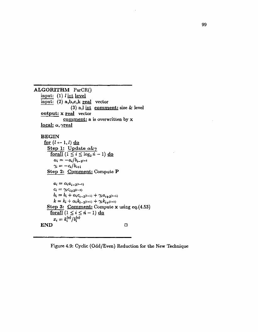
A L G O R IT H M ParCR() input: (1) I int level input: (2) a ,b ,c ,k real vector

(3) n,l int com m ent: size & level o u tp u t: x real vector

com m ent: a is overwritten by x local: a, ore a l

B E G IN for (/ <— 1 ,1) do

S tep 1: U p d a te ah~f forall (1 < i < log2 n — 1) do

oti = —a j /b ,- _ 2i - i

7« = - C i / k + i S tep 2: C om m ent: Compute P

Oj =c,- = 7,C,+2(l-1)6,- = bi -f- Q!jC^_2(l—l) -|- 7«®»+2(,—

k = ki + aik{_2(i-1) + Jiki+o-i)S tep 3: C om m ent: Compute x using eq.(4.53)

forall (1 < i < n — 1) do Xi = k ^ / b \ 9

E N D □

Figure 4.9: Cyclic (Odd/Even) Reduction for the New Technique

100

A L G O R IT H M New()B E G IN

S tep 1: Set / = 1. com m ent; level <— 1 S tep 2: Invoke P arC R . com m ent;

S tep 2.1; Solve resulting system using P arR DS tep 2.2; Substitute the results into original systemS tep 2.3; Repeat step 2 & 3 until final solution x is obtained

S tep 3 If / ^ log2 n — 1 then(a) Set I <— / + 1(b) goto step 2

E N D □

Figure 4.10; The New Algorithm Computing a Tridiagonal System at VariousReduction Levels

2. Five benchmarks algorithms, Gauss Elimination, LU and Orthogonal reduction,

Conjugate Gradient, and Symmetric Over-relaxation methods, are used to execute

the same model problem and their execution times compared to that of the new

algorithm. All but one of these benchmarks are parallelized. Gauss Elimination

algorithm is used in its serial form of its simplicity and elegance.

Chapter 5

Im plem entations and Experim ental R esults

The last thing one knows in constructing a work is.Blaise Pascal.

Concepts without percepts are empty. Percepts without concepts are blind.

Immanuel Kant.

The purpose of this chapter is two-fold: to give the implementation of the new

algorithm and its benchmarks on the MasPar MP-X (model 1208B), the com­

putational model whose architecture and hardware/software features immediately

relevant for our study were presented in chapter 2, and also to present the results

of this implementation and conclusion thereof. The implementation was carried

out in a series of experiments each of which involving the execution of the devel­

oped algorithms with different set of parameters. Data structures, such as deemed

appropriate to facilitate the implementation and to enhance an efficient inter-

processor communication and data routings needed, were developed and used in

all the experiments. The definition and implementation of the data structures are

treated in §5.1. The construction of the grid of the rectangular domain wherein

the model problem is approximated is treated in §5.2. The description of the ex­

periments and the determination of the parametric data used for conducting them

axe given in §5.3. The efficiency of the new algorithm execution was compared

to those of the benchmarks using three evaluation measures. One measure was

deviation of results of the algorithms — the new algorithm and the benchmarks —

from the exact solution. The exact solution was determined at the specific mesh

points of the domain where the the problem was approximated. The deviation

was measured in terms of average absolute error. The second evaluation measure

101

102

was the total cpu time required for each computation. The last measure was the

number of non-trivial floating point operations involved in each execution deter­

mined in terms of the mega flop (Mflops) rates of the computations concerned.

The implication of these results is duly discussed and the conclusion reached as

to whether the design and implementation of the new methodology was worth the

effort and, if so, to identify the computational situations that merit its application.

The results and the conclusion based upon the results are given in §5.4.

5.1 DATA STRUCTURES

There are various methods for storing sparse matrices in order to take advantage of

their structures. Several of these methods are only applicable for matrices of a par­

ticular form. For the matrices arising from the model problem used in this study,

two of such data structures were mentioned in §4.1. These are the straight and

row(column) interleaved storages which were used for demonstrating how nonzero

entries of matrix A could be handled in order to facilitate inter-processor commu­

nication and data routings called for in some computation situations, while, at the

same time, preventing the occurence of such common problems as fill-in and load-

imbalance. No particular parallel computer was envisaged in such discussions. In

this section, we give a more efficient data structuring that was used for the MasPar

MP-X programming.

Another commonly used data structure for sparse systems is the so-called di­

agonal storage. This storage scheme, when properly designed to take advantage of

the underlying hardware features of the particular parallel system, can be used for

efficient programming of any parallel processors — array, vector, or multiproces­

sors. One such modification might aim at making the storage scheme to be able

to handle a more general form of sparse systems. One common way to do that

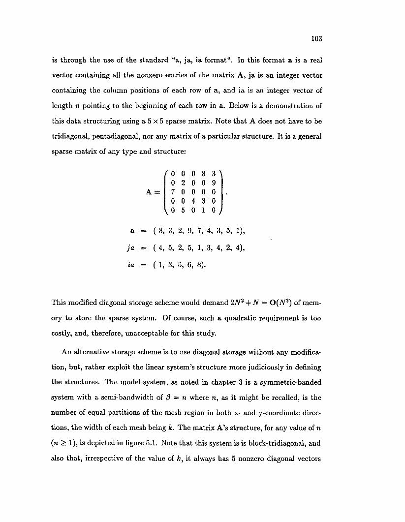
103

is through the use of the standard “a, ja, ia format". In this format a is a real

vector containing all the nonzero entries of the matrix A, ja is an integer vector

containing the column positions of each row of a, and ia is an integer vector of

length n pointing to the beginning of each row in a. Below is a demonstration of

this data structuring using a 5 x 5 sparse matrix. Note that A does not have to be

tridiagonal, pentadiagonal, nor any matrix of a particular structure. It is a general

sparse matrix of any type and structure:

( 0 0 0 8 3 \0 2 0 0 9

A — 7 0 0 0 00 0 4 3 0

l o 5 0 1 o )

a = (B, 3, 2, 9, 7, 4, 3,

ja = (4 , 5, 2, 5, 1, 3, 4,

ia = (1> 3, 5, 6, 8).

This modified diagonal storage scheme would demand 2N 2 + N = Q ( N 2) of mem­

ory to store the sparse system. Of course, such a quadratic requirement is too

costly, and, therefore, unacceptable for this study.

An alternative storage scheme is to use diagonal storage without any modifica­

tion, but, rather exploit the linear system’s structure more judiciously in defining

the structures. The model system, as noted in chapter 3 is a symmetric-banded

system with a semi-bandwidth of /? = n where n, as it might be recalled, is the

number of equal partitions of the mesh region in both x- and y-coordinate direc­

tions, the width of each mesh being k. The matrix A ’s structure, for any value of n

(n > 1), is depicted in figure 5.1. Note that this system is is block-tridiagonal, and

also that, irrespective of the value of &, it always has 5 nonzero diagonal vectors

104

1

Figure 5.1: Structure of Matrix A Resulting from Model Problem, /? = n

denoted in this report as d l, d2, d3, d4, and d5, where the main diagonal vector

is d3 and the nth subdiagonal vector dl. The rest of the vectors are indexed in

order as shown in figure 5.2.

In this study, these 5 diagonal vectors were defined and used as vexes (see chapter

2 for the meaning of a vex). As an example, for n — 3, the matrix A and the 5

vexes are:

/ - 4 1 1 0 \1 - 4 0 11 0 - 4 1

V 0 1 1 - 4 /

d l = ( 0, o, 1, 1)

d 2 = ( 0, 1, 0, 1)

d3 = ( - 4 , --4,

d4 = ( 10, 1, o)

d5 = ( 1 ,1 , 0, 0).

105

For general n, the pattern of storage for the 5 vexes is given below:

d l = (0 , 0, . . . , 0, 1, 1)<— n —►

d2 = (0 , 1, 1, 0, 1, 1 ,.. .)+— n —+

d3 = ( - 4 , - 4 , - 4 ) (5.1)— N —►

d4 = ( 1, 1, 0, 1, 1, 1, 0, . . . )

d5 = ( 1, 1, 1, 0, 0)<— n —►

The MPL code fragment that was used for defining the 5 vexes for a general value

of n is given in figure 5.2. Note that the matrix A is never stored explicitly. The

vexes are used for all computations involving A.

5.2 THE GRID CO NSTRUCTIO N

The rectangular domain (0,1) x (0,1) on which the model problem was approxi­

mated according to the approach discussed in chapter 3, was partitioned n times in

both the x — and y —coordinate directions and with the mesh width of k = , 7 , . , a («+!)’that is, n mesh lines in each direction. The resulting system was of dimension

N x N, where N = n2. Once n was determined, the grid coordinates were com­

puted using the MPL fragment in Figure 5.3 on page 107.

106

/* The following are the input parameters to this MPL code fragment: * /(a) N The system’s dimension(b) k The mesh width */(c) n The no. of partitions of mesh */

#include mpLh /* Must include this header file */{

plural double *dl,*d2,*d3,*d4,*d5; /* declares vexes*/ int nb, i; /* No. of memory layers , loop-counter */ double val /* temp, value */

nb = (n-l'Clnproc)-f-l /* nb determined based on value of n */d l = getstord(nb) d2 = getstord(nb) d3 = getstord(nb) d4 = getstord(nb) d5 = getstord(nb)

f* dynamic allocation of vex d l */ /* dynamic allocation of vex d2 * j I* dynamic allocation of vex d3 */ /* dynamic allocation of vex d4 * / /* dynamic allocation of vex d5 */

val=(double)-4; /* val = -4 */ p_vexcon(n, &val, (13, 0); /* dZ = (—4, —4 , . . . , —4) */p_vexcopy(n-n, d3, n, d5,0); /* d5 j= d3 */p_vexcopy(n-l, d3, 0, d2,l); /* d2 d3 */p_vexcopy(n-l, d3, 1, d4,l); /* d4 j = d3 */

val = (double) 0 /* val j= = 0 */for(i=0; ijn; i+=n){

p_vexput(&val, d2, i); /* introduces zero into d2 */p_vexput(&val, d4, i+n-1); /* introduces zero into d4 */

}

Figure 5.2: The Basic Data Structures and their Allocation

107

/* The following are the input parameters to this MPL code fragment: * / (a) n The system’s dimension (a) h The mesh width */

#include mpl.h /* Must include this header file */ # include ’’pmml.h”

{plural double *dl,*d2,*d3,*d4,*d5; /* declares vexes*/ plural double *x,*y; /* x &; y coords. * / double val /* temp, value */

nb = (n-l'C lnproc)+l /* nb determined based on value of n * / x = getstord(nb); /* dynamic allocation of vex x */ y = getstord(nb); /* dynamic allocation of vex y */

val=(double) 1; /* val = 1 * / p_vexcon(N, &val, d3, 0); /* d3 i= (1 ,... ,1) */p_vexinx(N, x, 0); /* u = (0 ,1 , . . . ,n — 1) * /p_vexcopy(N, x, 0, y,0); /* v j= u * /p_vexcopy(N, d3, 0, d2,l); /* ^2 j= d3 */p_vexcopy(N, d3, 1, d4,l); /* d4 j= d3 */p_vexfix(N, y, 0); /* fixes v in all layers */

val = (double) n /* val j== 0 * / p_vexaxpy(N, &k , y, 0, x, 0); /* x j= y*k */p_vexadd(N, d3, 0, x,0); /* x j= x+d3 */p.vexcal(N, &h, x, 0); /* x j= x*h */

}

Figure 5.3: The Mesh Region and the Mesh Point Coordinates

108

5.3 THE EXPERIM ENTS

5.3.1 The System Size D eterm ination and Usage

In chapter 2, we identified the computational model, namely, the MasPar MP-X,

for the solution of the model problem. We also discussed those hardware and

software features of this parallel processor, and, in particular, stated the fact that

the MasPar 1208B is actually half the size of the MPP, and that

® MasPar 1208B has 213 = 8192 processing elements or PEs in a 128 x 64

machine array,

• each PE has a local (nonshaxable) memory of size (PMEMSZ is MPL’s jar­

gon) of 216 = 65536 bytes.

In order to realize the maximum potential (in terms of parallelism) of this machine,

any program that executes on it should involve all the 8192 PEs. That is, for any

program to execute efficiently and with maximum parallelism, the program’s size

should be made to fit the machine size as closely as possible. In this study, we

determined the maximum n value that caused the model problem to fit exactly

the nyprocxnxproc processor array of the 1208B. That value was determined to

be 305 x 305 = 93025 using the following simple arithmetic calculation intermixed

with the MPL notation:

n = (int)sqrt((availm em <C lnproc)/(11.0*sizeof(double)));

(availm em = lOOOBytes.)

n = [(1000 x 2*3) -T- 88.0] 2 , (since ”double” type has size of 8 bytes.)

= 305, =*• JV = n2 = 3052 = 93025.

Thus, 305 is the maximum n value that caused the model problem to fit exactly

the machine size of 128 x 64 processors. That meant that the maximum number

109

of memory layers or blocks to accomodate the vexes was

n2 — 1 Inxproc = [93,000 -r- 128J = 726,

and the maximum number of layers for the veys was

n2 — 1 >• Inyproc = [93,000 -f- 64j = 1453.

5.3.2 Exact Solution

The mathematical model used in this study was the elliptic equation — Poisson’s

- that is given in eq.(3.15) whose independent variable u was approximated as U

with a 5-star stencil of the central finite difference approximation technique to give

eq.(3.20). The approximation of the Poisson’s equation was carried out on a square

domain (0,1) x (0,1) by first partitioning the domain in both coordinate directions

into n meshes of the same mesh width of k, and then applying the 5-star stencil

on each grid point ( i , j ) to produce eq.(3.20). Eqs.(3.15) and (3.20) are rewritten

out below as eqs.(5.2) and (5.3) respectively, for convenience:

_ f ( x y ) (52)

^Uij — Ui+i j — Ui-i j — Ui J+1 — U i j — l = k2f ( i j ) . (5.3)

The forcing function f ( x , y ) of the Poisson’s equation, eq.(5.2), can be any func­

tion, but, in this study, it was chosen to satisfy the Dirichlet boundary condi­

tions as specified in chapter 3. We solved eq.(5.3) in 2 ways. The first way was

generating the linear system of equations by expanding eq.(5.3) for grid point

(*>i)? V (i,j) € r i j n , where li is the square domain and T its boundary. In

other words, eq.(5.3) was written for the entire domain and its boundaries pro­

vided both the approximated function u(i, j) and the forcing function f ( i , j ) were

continuous in T U ^ . The choice of the function was such that both the

110

Dirichlet boundary conditions and the condition of continuity were satisfied. Once

eq.(5.3) was written for all the grid points, the linear system given in eq.(3.14) was

generated. The linear system was then solved by the methods discussed in chapter

4, in keeping with the objective of this study as given in chapter 1.

Another method of solving eq.(5.3) was by direct evaluation of U(i ,j) for each

grid point ( i , j ) by making use of the point’s position in the mesh (i.e., utilizing

its indices “i“ and “j “) and the fact of the the occurence of the constant coefficient

“-4“ for each point. Because the values of U at the 4 neighboring grid points must

be considered in computing the value of U for a given point this computation

was carried out in serial using the MPL fragment given in Figure 5.4. The results

of this computation were the exact solution of U at all the grid points. As we will

explain shortly, the exact solution was used in determining the average absolute

errors associated with the determining the solution of the linear system by the

algorithms developed in chapter 4.

5.3.3 Experim ental Approach

An investigation of the efficiency and the applicability of the new method in solving

the model problem was conducted by executing both the new algorithm and its

benchmarks, and then comparing all the results of the executions using the three

evaluation metrics mentioned in the introduction of this chapter. A total of 4

experiments were conducted each involving one of the system incremental size

(N ) of 1600,10000,40000, and 93025, that is, at the n values of 40,100,200, and

305 respectively. In the case of the new algorithm, only the maximum level of

reduction, that is, \log(Ny\ — 1, of the cyclic reduction (ParCR() of Figure 4.13)

was used.

I l l

The results of the various executions were compared with those of the exact

solution which were computed per grid point using the MPL fragment provided in

Figure 5.4. The benchmark results were compaxed to those of the new approach

using the three evaluation metrics — average absolute error, cpu times, and mega

flop rates.

The preprocessing step which used the LU factorization to reduce matrix A

into L and U before using the parallel recursive doubling (ParRD() of Figure 4.12)

was not included in the determination of the evaluation metrics. That is, only the

linear recursion of eq.(4.36) was determined using the recursive doubling algorithm,

ParRDQ (Figure 4.12), and the operations involved in that determination were

considered in the evaluation measure, while the nonlinear recursion of eq.(4.33)

was not solved by the recursive doubling technique but was computed serially as

a preprocessing step, and, as such, its computations were not considered in the

evaluation measure determination.

All the data structures used were represented as the MasPar MPL data struc­

tures which are vex, vey and mat. Also, to ensure efficiency of computation, the

MasPar MPLABB routines were used as much as possible.

5.4 EXPERIM ENTAL RESULTS

Given in Figures 5.5 - 5.8 are the results obtained by executing the model problem

at the system sizes of 1600, 10000,40000 and 93025 respectively. Tables 5.1 - 5.4

give the comparison of the results in terms of average absolute errors with respect

to the exact solution. The exact solution was determined by computing the values

of the dependent variable U at all the grid points. Figures 5.9 and 5.10 give the

cpu times and the mega flop rates of the respective execution. In all the figures

and tables of the results, the keys "Exact Soln” , "New”, "SOR”, ”GE” , ”CG” , and

112

”Ortho” stand for the computational result of exact, Symmetric-Overrelaxation,

Gauss Elimination, Conjugate Gradient, and Orthogonal methods respectively.

The orthogonal reduction used was the Householder factorization as explained in

chapter 4. The LU reduction was not used as a benchmark since, as explained in

§4.1, it is equivalent to the GE method, but, as stated above, the LU reduction

was involved in the preprocessing step of the recursive doubling algorithm. Of the

benchmarks, only the GE method was used as a serial code for the reason already

given in §4.1 — serial usage is simple and elegant and the benefits that accrue from

the parallel implementation of GE axe miniscule, hence, in many applications of

GE given in the literature, serial implementation of GE is are the rule. The rest

of the benchmarks, however, were implemented in parallel in accordance with the

steps of their respective pseudocoded algorithms given in chapter 4.

5.4.1 R esults and Observations

Below are some of the most obvious observations that can be made from the results:

O bservation 1: The results shown in Figures 5.5 - 5.9, even by visual inspection,

seem reasonable approximations of the values of U at the indicated grid points as

they appear to satisfy the Dirichlet boundary conditions which were specified to be

zero at the four sides of the rectangular domain. That is, u(x,y) = 0, V(x,y) £ T,

where, as may be recalled from chapter 3, T was the set of the boundary points

of the domain. Since the values of U, according to the boundary conditions, were

zero at the boundaries, one would expect the results, at least, to tend to this value

at the boundaries. An examination of Figures 5.5 - 5.8 indicates that such is the

case. Note that n was the width of the domain in the two coordinate directions.

Hence, at an integral multiples of n, the values of U clustered about zero.

113

/* The following axe the input parameters to this MPL code fragment: * /(a) dl,d3 The vexes determined in code of fig.5.2 * /(b) N The size of the system * /

(c) n The no. of partitions of mesh */

(d) x , y /* x k y vexes. */

# include mpl.h /* Must include this header file */{

plural double *dl, *d3, *x, *y; /* declares d3 vex*/ plural double *u; /* declares exact u vex */ int nb, i; /* No. of memory layers , loop-counter */ double val /* temp, value */

nb = (N-l'Clnproc)-f 1 /* nb determined based on value of n * / d3 = getstord(nb); /* dynamic allocation of vex d l * / ujexact = getstord(nb); /* dynamic allocation of vex exact u * /

val=(double) 1; /* val = 1 */p_vexcon(n, &val, u_exact, 0); /* ujexact = ( 1 ,1 , . . . , 1) */p_vexsub(N, y, 0, u_exact,0); /* u_exact j= 1-y */ p_vexmul(N, y, 0, u_exact,0); /* u_exact j= y(l-y) * / p_vexcon(N, &val, d l, 0); /* d l = (1 ,1 , .. . , 1) */p_vexsub(N, x, 0, dl,0); /* d l j= 1-x */p_vexmul(N, x, 0, u_exact,0); /* u.exact j= x * / p_vexmul(N, d l, 0, ujexact,0); /* u_exact * /

}

Figure 5.4: The Exact Solution of the Model Problem

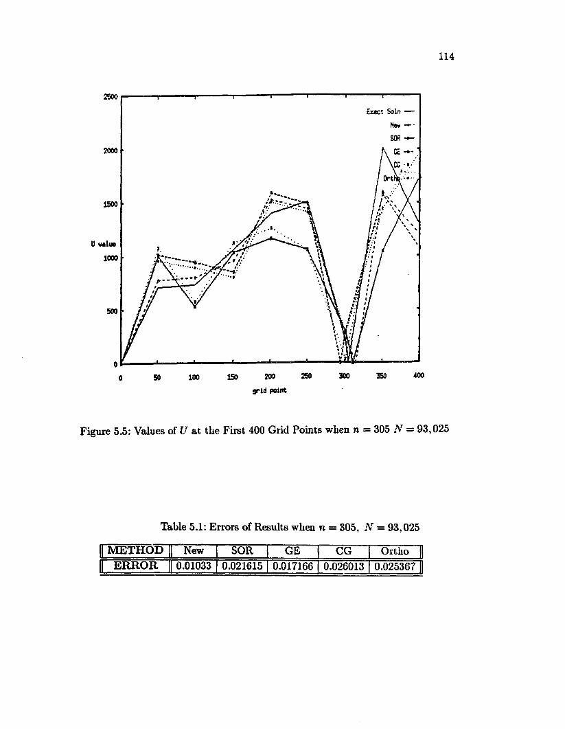
114

2500

2000

Ortl

\V

1500

1000

500

400250 350200ISO50 1000grid point

Figure 5.5: Values of U a t the First 400 Grid Points when n = 305 N = 93,025

Table 5.1: Errors of Results when n = 305, N = 93,025

M E T H O D New SOR GE CG OrthoE R R O R 0.01033 0.021615 0.017166 0.026013 0.025367

115

2500

2000

1500

500

250 900 400150 200 350100500grid point

Figure 5.6: Values of U a t the First 400 Grid Points when n = 200, Ar = 40,000

Table 5.2: Errors of Results when n = 200, N — 40,000

M E T H O D New SOR GE CG OrthoE R R O R 0.016102 0.021992 0.030503 0.034183 0.029903

2500

2000

1500

U value

1000

500

00 SO 100 150 200 250 300 350 400

grid point

Figure 5.7: Values of U at the First 400 Grid Points when n = 100, Ar = 10,000

Table 5.3: Errors of Results when n — 100, N = 10,000

M E T H O D New SOR GE CG OrthoE R R O R 0.024933 0.025965 0.031008 0.035128 0.026581

Exact Soln —-

HawX

117

1600Exact So In - —

1400

1200

800

U value

600

400

200

160 200ISO14080GO20 409*1(1 point

Figure 5.8: Values of U at the First 200 Grid Points when n = 40, N = 1,600

Table 5.4: Errors of Results when n = 40, N = 1,600

M E T H O D New SOR GE CG OrthoE R R O R 0.025323 0.027955 0.038929 0.039192 0.027404

118

Now •*SOR -►

cpu tine

0 10000 20000 30000 40000 50000 60090 70000 80000 90000 100000

size N

Figure 5.9: CPU Times of the Algorithms

119

/GE - - CG •*-

Ortho

19000 20000 30000 40000 50000 60000 70000 BOOOO 90000 10000C0

liza N

Figure 5.10: Megaflop Rates of the Algorithms

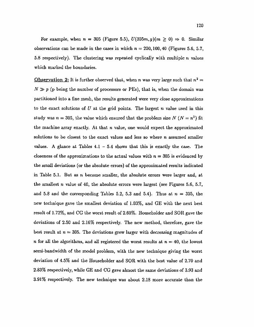
120

For example, when n = 305 (Figure 5.5), U(305m,y)(m > 0) 0. Similar

observations can be made in the cases in which n = 200,100,40 (Figures 5.6, 5.7,

5.8 respectively). The clustering was repeated cyclically with multiple n values

which marked the boundaries.

O bservation 2: It is further observed that, when n was very large such that ra2 =

iV » p (p being the number of processors or PEs), that is, when the domain was

partitioned into a fine mesh, the results generated were very close approximations

to the exact solutions of U at the grid points. The largest n value used in this

study was n = 305, the value which ensured that the problem size N (N = n2) fit

the machine array exactly. At that n value, one would expect the approximated

solutions to be closest to the exact values and less so where n assumed smaller

values. A glance at Tables 4.1 - 5.4 shows that this is exactly the case. The

closeness of the approximations to the actual values with n = 305 is evidenced by

the small deviations (or the absolute errors) of the approximated results indicated

in Table 5.1. But as n became smaller, the absolute errors were larger and, at

the smallest n value of 40, the absolute errors were largest (see Figures 5.6, 5.7,

and 5.8 and the corresponding Tables 5.2, 5.3 and 5.4). Thus at n = 305, the

new technique gave the smallest deviation of 1.03%, and GE with the next best

result of 1.72%, and CG the worst result of 2.60%. Householder and SOR gave the

deviations of 2.50 and 2.16% respectively. The new method, therefore, gave the

best result at n = 305. The deviations grew larger with decreasing magnitudes of

n for all the algorithms, and all registered the worst results at n = 40, the lowest

semi-bandwidth of the model problem, with the new technique giving the worst

deviation of 4.5% and the Householder and SOR with the best value of 2.70 and

2.83% respectively, while GE and CG gave almost the same deviations of 3.93 and

3.91% respectively. The new technique was about 2.18 more accurate than the

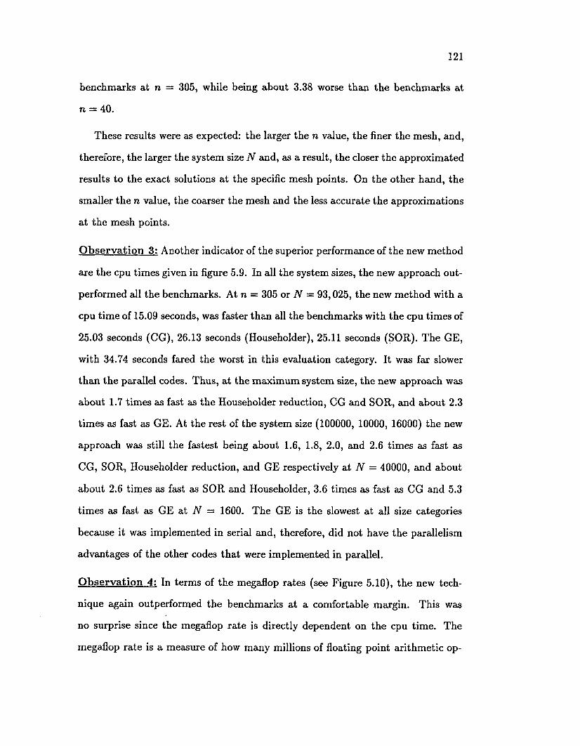
121

benchmarks at n = 305, while being about 3.38 worse than the benchmarks at

n = 40.

These results were as expected: the larger the n value, the finer the mesh, and,

therefore, the larger the system size N and, as a result, the closer the approximated

results to the exact solutions at the specific mesh points. On the other hand, the

smaller the n value, the coarser the mesh and the less accurate the approximations

at the mesh points.

O bservation 3: Another indicator of the superior performance of the new method

are the cpu times given in figure 5.9. In all the system sizes, the new approach out­

performed all the benchmarks. At n = 305 or N = 93,025, the new method with a

cpu time of 15.09 seconds, was faster than all the benchmarks with the cpu times of

25.03 seconds (CG), 26.13 seconds (Householder), 25.11 seconds (SOR). The GE,

with 34.74 seconds fared the worst in this evaluation category. It was far slower

than the parallel codes. Thus, at the maximum system size, the new approach was

about 1.7 times as fast as the Householder reduction, CG and SOR, and about 2.3

times as fast as GE. At the rest of the system size (100000, 10000, 16000) the new

approach was still the fastest being about 1.6, 1.8, 2.0, and 2.6 times as fast as

CG, SOR, Householder reduction, and GE respectively at N = 40000, and about

about 2.6 times as fast as SOR and Householder, 3.6 times as fast as CG and 5.3

times as fast as GE at N = 1600. The GE is the slowest at all size categories

because it was implemented in serial and, therefore, did not have the parallelism

advantages of the other codes that were implemented in parallel.

O bservation 4: In terms of the megaflop rates (see Figure 5.10), the new tech­

nique again outperformed the benchmarks at a comfortable margin. This was

no surprise since the megaflop rate is directly dependent on the cpu time. The

megaflop rate is a measure of how many millions of floating point arithmetic op­

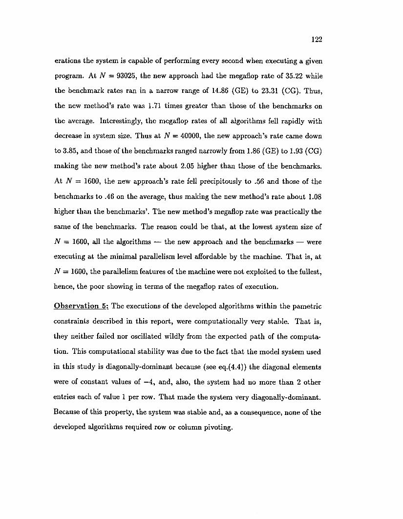
122

erations the system is capable of performing every second when executing a given

program. At N = 93025, the new approach had the megaflop rate of 35.22 while

the benchmark rates ran in a narrow range of 14.86 (GE) to 23.31 (CG). Thus,

the new method’s rate was 1.71 times greater than those of the benchmarks on

the average. Interestingly, the megaflop rates of all algorithms fell rapidly with

decrease in system size. Thus at N = 40000, the new approach’s rate came down

to 3.85, and those of the benchmarks ranged narrowly from 1.86 (GE) to 1.93 (CG)

making the new method’s rate about 2.05 higher than those of the benchmarks.

At N = 1600, the new approach’s rate fell precipitously to .56 and those of the

benchmarks to .46 on the average, thus making the new method’s rate about 1.08

higher than the benchmarks’. The new method’s megaflop rate was practically the

same of the benchmarks. The reason could be that, at the lowest system size of

N = 1600, all the algorithms — the new approach and the benchmarks — were

executing at the minimal parallelism level affordable by the machine. That is, at

N = 1600, the parallelism features of the machine were not exploited to the fullest,

hence, the poor showing in terms of the megaflop rates of execution.

O bservation 5: The executions of the developed algorithms within the pametric

constraints described in this report, were computationally very stable. That is,

they neither failed nor oscillated wildly from the expected path of the computa­

tion. This computational stability was due to the fact that the model system used

in this study is diagonally-dominant because (see eq.(4.4)) the diagonal elements

were of constant values of —4, and, also, the system had no more than 2 other

entries each of value 1 per row. That made the system very diagonally-dominant.

Because of this property, the system was stable and, as a consequence, none of the

developed algorithms required row or column pivoting.

123

From the above observations, it is obvious that the new technique faxed better

than all the benchmarks when N >• 8,192, as was the case when N = 93025,10000,

and 10000, but did not do as well in all the three evaluation measures when

N < 1600. The superior computational capability of the new technique which

manifested in the the above results was due to a number of factors some of which

were hinted in the discussion above. We summarize the most salient of these factors

below:

1. The new technique was designed by combining two powerful algorithmic tools

— cyclic reduction and recursive doubling — to execute the model problem.

The Cyclic reduction method, although it was not designed originally for

parallel computing, has considerable inherent parallelism. When used with

such auxiliary algorithms as the Gaussian elimination, the Choleski decom­

position or other factorization techniques, the cyclic reduction can be a very

effective tool for solving linear systems of equations, not just the type of sys­

tem modeled for this study. The maximum benefits of the cyclic reduction are

realizable when the algorithm is well designed even if the auxiliaxies are im­

plemented serially as is usually the case. Some of these auxiliary algorithms

involve recursions which, without the benefit of such other techniques as re­

cursive doubling to solve them in parallel, must be solved sequentially. When

recursions are computed in parallel by the auxiliary, the use of the auxiliary

with the cyclic reduction technique can potentially be very effective parallel

algorithm. The combination of the cyclic reduction and recursive doubling

technique to design a new algorithm is what this study set out to achieve.

In this study, the auxiliary algorithm was the LU factorization method the

linear recursions of which was handled in parallel by the recursive doubling

method.

124

From the indicated results and observations, we conclude that the new algo­

rithm, is a very computationally effective tool for solving the model problem

when the size of the system solved is very large or when the system size fits

the machine array.

2. MasPar 1208B, just like any parallel processor, performs at the peak of its

computational capability when all the processing elements are involved in

computing, which, in the context of our experiments, means having the sys­

tem size to be a lot larger than the 8,192 processing elements. Under this

cicumstance, one would expect the highest system’s performance in terms

of the cpu times, the mega flop rates. According to the above observations,

such was the case with the sizes 63025,40000, and 10000 since these were

significantly greater than 8192, the total number of PEs of MasPar model

1208B. There was a clear degradation in performance of the new algorithm

when the size of 1600 was used. The explanation is that, with high N value,

there was a better utilization of the machine as many PEs became involved

in the computation. That is, the load-imbalance problem, though it existed

in all levels of computation of the algorithms proposed in this study, did not

have a very damaging effect on the performance at the three high N values

as it it did when the size was 1,600 or lower (results for N, 1,600 are not

shown).

3. Both the recursive doubling and the cyclic reduction techniques which form

the core of the new algorithmic technique utilized O \og2(N) operations while

each of the benchmarks required significant more operational steps, for ex­

ample, the exhobitant 0 ( N 3) operations by the GE (see §4.1.1A).

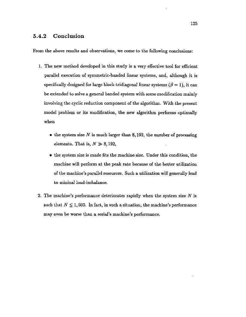
125

5.4.2 Conclusion

From the above results and observations, we come to the following conclusions:

1. The new method developed in this study is a very effective tool for efficient

parallel execution of symmetric-banded linear systems, and, although it is

specifically designed for large block-tridiagonal linear systems (/? = 1), it can

be extended to solve a general banded system with some modification mainly

involving the cyclic reduction component of the algorithm. With the present

model problem or its modification, the new algorithm performs optimally

when

• the system size N is much larger than 8,192, the number of processing

elements. That is, N 8,192,

• the system size is made fits the machine size. Under this condition, the

machine will perform at the peak rate because of the better utilization

of the machine’s parallel resources. Such a utilization will generally lead

to mininal load-imbalance.

2. The machine’s performance deteriorates rapidly when the system size N is

such that N < 1,600. In fact, in such a situation, the machine’s performance

may even be worse than a serial’s machine’s performance.

Bibliography

[AKE 89]

[AKI 89]

[ALMASI 89]

[AMES 77]

[ANDER 89]

[BATCH 74]

[BATCH 82]

[BAUCOM 88]

[BELL 85]

[BELYT 84]

[BELYT 87]

Ake, B., D ifference M eth o d s — Solu tions of E qua tions in R 11, Handbook of Numerical Analysis, Elsevier Pub., 1989.

Aki, S.G., T h e D esign and A nalysis o f P ara lle l Algo­r ith m s, Prentice-Hall, Inc. , New Jersey.

Almasi, G.S., et al., H ighly P ara lle l C o m pu ting , Benjamin- Cumming, Redwood City, CA.

Ames, W.F., N um erical M eth o d s for P a r tia l D ifferential E qua tions, Academic Press, Inc., New York, (1977).

Anderson, E., and Y. Saad, Solving Large T riangu lar Sys­tem s on P ara lle l C o m p u ters,In t’l. Jour. High Speed Comp, , pp. 73-96.

Batcher, K., STA R A N P ara lle l P ro cesso r S ystem H an d ­book , AFIPS Conf. , AFIPS Proc. 43, NCC, (1974), pp. 405- 410..

Batcher, K., M P P : A S u p ersy stem for sa te llite Im age P rocessing , 1982 Nat. Comp. Conf. (AFIPS), 51.

Baucomb, C. L., R educed S ystem s and th e P reco n d i­tio n ed C on jugate G rad ien t M e th o d on a M u ltip ro ces­sor, M.S. Thesis, Dept, of Comp. Sci. , Univ. of Illinois at Urbana-Champaign, (1988).

Bell, C. G., M ultis: A N ew C lass o f M u ltip ro cesso r C om ­p u te rs ,Science, 228, (1985), pp. 462-467.

Belytschko, M. , et al., H ourglass C ontro l in L inear and N on linear P ro g ram s, Comp. Meth. in Appl. Mech. and Eng., 43, (1984), pp. 251-276.

Belytschko, M., and N.Gilbertsen, C o n cu rren t an d V ector­ized M ixed T im e, E xp lic it N on linear S tru c tu ra l D y­nam ics A lgorithm , In Parallel Computations and Their Im­pact on Mechanics ed., ASME, New York, pp. 280-291.

126

127

[BELYT 89]

[BIRK 83]

[BISCHOF 83]

[BOIS 72]

[BOUK 72]

[BURN 88]

[BUZBEE 70]

[CHAZAN 69]

[COLE 84]

[DADDY 92]

[DASGUP 89a]

[DASGUP 89b]

[DIGIT 81a]

[DIGIT 81b]

Belytschko, M., et al. , P ara lle l P rocesso rs and N on linear S tru c tu ra l D ynam ics A lgorithm s Softw are, Semiannual Progress Report, (DEc. 1988-May 1989).

Birkhoff, G., and R.E. Lynch, N um erica l S o lu tion of E llip ­tic P rob lem s, SIAM Pub. , (1983).

Bischof, C.H., A B lock Q R F acto riza tion A lgo rithm U sing R e s tric ted P ivo ting , Journ. of Supercomp, (1989), pp.248- 257.

Boisvert, R.F., and R.A. Sweet, Sources and D evelopm ent o f M ath em a tica l Softw are, In W. Cowell ed. , Prentice-Hall, Inc. Englewood Cliffs, New Jersey, (1982).

Bouknight, H. , et al., T h e Illiac IV S ystem , Proc. IEEE, 60, (1972), pp. 369-379., Reading, Ma.

Bouknight, D.S., F in ite E lem en t A nalysis: F rom C on­cep ts to A pplications, Addison-Wesley, New Jersey, (1988).

Buzbee, B .L ., et al., On D irec t M eth o d s for Solving Pois­son’s E qua tion , SIAM Jour. Num. Anal., 7, pp. 627-656.

Chazan, D., and W. Miranker C hao tic R elaxa tion , Linear Algebra & its Applications, 2, (1969), pp. 199-222.

Coleman, T.F., Large Sparse N um erical O p tim iza tion , Lecture Notes in Computer Science, 165, Springer-Verlag, New York, (1984).

Daddy, W.L., M echanism s for C o n cu rren t C om puting , Int’l, Conf. on the 5th Gen. Syst., pp. 154-156.

Dasgupta, S., C o m p u te r A rch itec tu re : A M o d ern Syn­thesis, Vol. 1, John Wiley &; Sons, Inc.

Dasgupta, S., C o m p u te r A rch itec tu re : A M o d ern Syn­thesis,Vol. 2, John Wiley & Sons Inc.

T h e VAX A rch itec tu re H andbook , Digital Equipment Cor­poration, Maynard, MASS.

T h e VAX A rch itec tu re H andbook , Digital Equipment Cor­poration, Maynard, MASS.

128

[DIGIT 85]

[DONGA 86]

[DUNCAN 90]

[EAGER 89]

[FLYNN 66]

[FLYNN 72]

[FOX 86]

[GARVEY 93]

[GEUDER 93]

[GILM 71]

[GILOI 81]

[GILM 83]

T he VAX 8600 P rocessor, Digital Technical Jour. , Digital Equipment Corporation, Hudson, MASS.

Dongara, J .J., A Survey of H igh -P erfo rm ance C o m p u t­ers, Digest of papers: IEEE Com. Soc. COMCON, (Spring 1986), pp. 8-11.

Duncan, R., A Survey of P aralle l C o m p u te r A rch itec­tu re s , 23, No.2, (Feb. 1990), pp. 5-16.

Eager, D.L., et a l . , S peedup V ersus Efficiency in P aralle l System s, IEEE Trans, on Comp., C-38, No. 3, (1989), pp. 408-423.

Flynn, M., V ery H igh Speed C o m puting S ystem s, Proc. IEEE, 54, pp. 1901-1909.

Flynn, M ., Som e C o m p u te r O rganizations and T h e ir Dif­ferences, IEEE Trans. Comp. C-21, (1972), pp. 948-960.

Fox, G., Q uestions and U nexpected A nsw ers in C oncur­ren t C om p u ta tio n , Tech. Rep. No. CP-288, CAL Tech. Con- curr. Comp. Prog., CALTECH, Jet Propulsion Labs, Pasadena, Cal.

Garvey, S.D., A n Efficient M eth o d for Solving th e E igen­value P ro b lem for M atrices H aving A Skew -Sym m etric (or Skew -H erm itian) C om ponen t of Low R ank , Int’l Jour, for Num. Meth. in Eng., 36, (1993), pp. 4151-4163.

Geuder, U. , et al., G R ID S U ser’s G uide, Computer Science Report, (April 1993), Comp. Sci. Dept., Univ. of Stuttgart, Germany.

Gilmore, P., N um erical Solu tion of P a r tia l D ifferential E qua tions by A ssociation P rocessing , Proc. FJCL, AFIPS Press, Montvale, New Jersey, (1971), pp. 411-418.

Giloi, W.K., A C om plete Taxonom y of C o m p u te r A r­ch itec tu re B ased on th e A bso lu te D a ta T ype View, In Blaauw & Handler ed., (1981), pp. 19-38.

Gilmore, P., T he M assively P aralle l P ro cesso r (M P P ): A Large Scale SIM D P rocessor, Proc. of SPIE, 431, (Aug. 1983).

129

[GILOI 83]

[GLAD 79]

[GOLUB 93]

[GOODMN 81]

[GOLD 72]

[FOX 86]

[GOODYR 74]

[GRIT 88]

[GUSEV 91]

[GUSEV 92a]

[GUSEV 92b]

Giloi, W.K., Towards a Taxonom y of C o m p u te r A rchi­te c tu re B ased on th e M achine D a ta T y p e V iew , Proc. of the 10th Annual Int’l. Symp. on Comp. Arch., IEEE. Comp. Soc. Press, New York, (1983), pp. 6-15.

Gladwell, J., and R. Wait, A Survey of N um erica l M e th ­ods for P a r tia l D ifferential E quations, Oxford Univ. Press, (1979).

Golub, G. and J.M. Ortega, Scientific C om puting : A n In ­tro d u c tio n W ith P ara lle l C om pu ting , Academic Press, Inc. , Boston and New York.

Goodman, J.R., and C.H Sequin, H y p e rtree : A M u ltip ro ­cessor In te rco n n ec tio n Topology, IEEE Trans. Comp., C- 303, No. 12, (Dec. 1981), pp. 923-933.

Goldstine, H.H., T h e C o m p u te r from Pascal to von N eu­m ann, Princeton University Press, Princeton, New Jersey, (1972).

Goodman, J.R., and C.H. Sequin, H y p e rtre e : A M u ltip ro ­cessor In te rconnection .

A pplication of STA R A N to Fast F ourier T ransform s , Report GER 16109, (May 1972).

Grit, D.H., and J.R. McGraw, P ro g ram m in g D ivide- and C onquer for a M IM D M echine, Softw. Prac. and Exper., 15, No. 1, (1988), pp. 41-53.

Gu{eev, M., and D.J. Evans, Som e N o n lin ear T ransfo rm a­tio n of M a tr ix V ector M u ltip lica tio n A lgo rithm , Tech. Rep., 635, Loughborough Univ. of Tech., PARC, Dept, of Comp. Stud., (Oct. 1991).

Gu{eev, M., and D.J. Evans, A Fast Sym bolic D esign and D ouble P ipe lines, Tech. Rep., 665, Loughborough Univ. of Tech., PARC, Dept, of Comp. Stud., (Jan. 1992).

Gu{eev, M., and D.J. Evans, Speed ing up th e Systolic D e­sign in th e B id irectional L inear A rrays, Tech. Rep., T02, Loughborough Univ. of Tech., PARC, Dept, of Comp. Stud., (April 1992).

130

[HAND]

[HAYNES 82]

[HELLER 78]

[HEUB 82]

[HENSY 91]

[HOCK 65]

[HOCK 70]

[HOCK 81]

[HOCK 87]

[HOCK 88]

[HOLL 93]

[HWANG 84]

[HWANG 87]

Handler, W., T h e Im p a c t o f C lassification Schem es on C o m p u te r A rch itec tu re” , Proc. of the 1977 Int’l Conf. on Par. Proc., (1977), pp. 7-15.

Haynes, L. et al., A Survey of H igh ly P ara lle l , Computer, 15, No. 1, (Jan. 1982), pp. 9-24.

Heller, D., A Survey of P ara lle l A lgo rithm s in N um erical L inear A lgebra, SIAM Rev. 20, (Oct. 1978), pp. 740-777.

Heuber, K.H., and E.A. Thornton, T h e F in ite E lem en t M eth o d fo r E ngineers, John Wiley & Sons, Inc. (1982).

Hennessy, J.L., and N.P. Jouppi, C o m p u te r Technology and A rch itec tu re : A n Evolving In te ra c tio n , C o m p u te r and A rtificial In te lligence, McGraw-Hill Bk. Co., New York.

Hockney, R.W., A Fast D irec t S olu tion of P o isson’s E qua­tio n U sing F ourier A nalysis, J. ACM,12, (march 1965), pp. 95-113.

Hockney, R.W., T h e P o ten tia l C alcu la tion an d Som e A p­plications, Meth. Comp. Phys., 9, pp.135-211.

Hockney, R.W., and J.W. Eastwood, C o m p u te r S im ulation U sing P aritic les , McGraw-Hill Pub. Co., Inc., New York,(1981).

Hockney, R.W., C lassification and E va lua tion of P ara lle l C o m p u te r System s, In Springer-Verlag Notes in Comp. Sci., No. 295, (1987), pp. 13-25.

Hockney, R. and C.Jesshope, P ara lle l C o m p u ters, Adam- Hilger, Bristol and Philadelphia.

Hollingsworth, R., A dvanced S em iconducto r Technology, Comm. ACM, 36, No. 2, (Feb. 1993), pp. 83-105.

Hwang, K., and F.A. Briggs, C o m p u te r A rch itec tu re and P ara lle l P rocessing , McGraw-Hill Pub. Co., New York.

Hwang, K., and J. Ghosh, H y p ern e t: A C om m unication- Efficient A rch itec tu re for C o n stru c tin g M assively P a r­allel C o m p u ters , IEEE Trans. Comp., (Dec. 1987).

131

[HWANG 89]

[KUCK 77]

[KUCK 82]

[LAMBIO 75]

[LEIGH 92]

[LEVES 90]

[LOHNER 93]

[MACK 87]

[MAYR 69]

[MPPE]

[MPPSYS]

[MPPPLS]

[MPML]

Hwang, K., and F. Degroot, P ara lle l P rocessing for S u p er­co m p u ters and A rtificial In te lligence , McGraw-Hill Pub. Co., New York.

Kuck, D.J., P ara lle l P rocessing of O rd in a ry P rog ram s, Advances in Computers, 15, Academic Press, New York, (1977), pp. 119-179.

Kuck, D.J., and R. Stokes, T h e B urroughs Scietific P ro ­cessor (B S P ), IEEE Trans. Comp. , C-31, pp. 363-376.

Lambiotte, J., T h e S olu tion of L inear S ystem s of E q u a­tions on a V ector C o m p u ter, Ph.D Diss., Univ. Virginia, Charlottesville.

Leighton, F. T., In tro d u c tio n to P ara lle l A lgo rithm s and A rch itec tu res : A rrays, T rees, H y p e rtree s Morgan Kauff- mann, (1992).

Levesque, J.M., A P ara lle l P ro g ram m in g E nv ironm ent, IEEE Par. Prog., (1990), pp. 291-294.

LOhner, R.I., Som e Useful R en u m b erin g S tra teg ies for U n s tru c tu re d G R ID S, Int’l. Jour, for Num. Meth. in Eng., 36, (June 1993), pp. 3259-3270.

Mackintosh, A. R., and W. Miranker T he F irs t E lec tron ic C o m p u ter, Physics Today, (March 1987), pp. 25-32.

Mayr, E., P rinc ip les of S y stem atic Zoology, McGraw-Hill Pub. Co., New York.

M asP ar P ro g ram m in g E n v iro n m en t (M P P E ), Softwr. version 2.2, Document Part No. 9305-0000, Rev.A6, (Dec., 1991).

M asP ar S ystem O verview , Document Part No. 9300-0100, Rev.A4, (Dec., 1991).

M asP ar P ro g ram m in g Language (A N SI C om patib le M P L ), Softwr. ver.2.2, Document Part No. 9302-0001, Rev.Al, (Dec., 1991).

M asP ar M asP ar M ath e m a tics L ib rary (M P M L ), Softwr. ver.2.2, Document Part No. 9302-0400, Rev.A3, (Dec., 1991).

132

[MPCMDS]

[METRO 80]

[MIKLOS 84]

[MIRAN 71]

[MODI 88]

[MORSE 78]

[MURA 71]

[NIEVER 64]

[ORTEGA 85]

[ORTEGA 88]

[ORTIZ 89]

[ORTIZ 86]

[PEASE 74]

M asP ar M asP ar C om m ands R eference M anual, Softwr. ver.2.2, Document Part No. 9302-0300, Rev.A7, (Dec., 1991).

Metropolis, N., and J. Worlton, A Trilogy on E rro rs in th e H is to ry of C om puting , Annals Hist, oc Comp., 2, No. 1, pp. 49-59.

Miklosko, J., and V.E. Kotov, A lgorithm s, Softw are & H ardw are o f P ara lle l C o m p u ters, Springer-Verlag, (1984), New York.

Miranker, W., A Survey of P ara lle lism in N um erical A nal­ysis, SIAM Rev., 13, (1971), pp. 524-547.

Modi, J. J., P ara lle l A lgo rithm s and M a trix C o m p u ta ­tions, Clarendon Press, Oxford, UK, (1988).

Morse, S. P. , et al., In te l M icroprocessors: 8008 to 8086, Intel Corporation, Aloha, OR, Reprinted in Siewiorek, Bell, and Newell (1982), pp. 615-642.

Muraoka, Y., P ara lle lism E xposu re and E x p lo ita tio n in P rog ram s, Tech. Report No. 71-424, Comp. Sci. Dept., Univ. of Illinois, (1971).

Nievergelt, J., P ara lle l M eth o d s for in teg ra tin g O rd in ary D ifferential E quations, Comm. ACM, 7, (1964), pp. 737-743.

Ortega, J.M., and G. Voigt, Solu tion of P a r tia l D ifferential E qua tions on V ector and P ara lle l C o m p u ters , A Survey, SIAM Rev., 27, No. 2, (June 1985), pp. 149-290.

Ortega, J.M., In tro d u c tio n to P ara lle l and V ector Solu­tio n of L inear System s, Plennum Press, New York.

Ortiz, M., C o n cu rren t A lgorithm s for T ransien t N onlin ­ea r F in ite E lem en t A nalysis, Tech. Report, Div. of Eng. Brown Univ. Rhode Island.

Ortiz, M., and B. Nour-Omid, U nconditional S tab le Con­c u rren t P ro ced u res for T ransien t F in ite E lem en t A nal­ysis, Comp. Meth. Appl. Mech., 58, pp. 151-174.

Pease, M.C., , T h e C (2 ,m ) A lgo rithm for M a tr ix Inver­sion, Tech. Rep., Stanford Res. Inst., Menlo Pork, CA, (1974).

133

[RAND 75]

[RICE 83]

[ROSS 74]

[RUDOL 72]

[RUSS 73]

[SCHAE 77]

[SCHW 83]

[SCHUM 76]

[SIEWIO 82]

[SKILL 88]

[SOKAL 63]

[STONE 73]

[STONE 80]

[STONE 90]

Randell, B., O rigins o f D igital C o m p u ters, Springer-Verlag, New York, (1975).

Rice, J.R., N u m erical M ethods, Softw are, and A nalysis, In IML Reference ed., McGraw-Hill Pub. Co., (1983).

Ross, H.H., Biological S ystem atics, Addison-Wesley, Read­ing, MA.

Rudolph, J., A p ro d u c tio n Im p lem en ta tio n of an A ssocia­tiv e A rray P ro cesso r - STA R A N , Proc. Fall Joint Comp. Conf., AFIPS Press, Montvale, NJ, (1972), pp. 229-241..

Ruse, M., T h e Philosophy of Biology, Hutchinson Univ. Lib., London.

Schaefer, D.H. and J.P. Strong, T se C om pu ters, Proc. of the IEEE, 65, No. 1, (Jan. 1977).

Schwartz, J., A Taxonom y Table o f P ara lle l C o m p u ters, B ased on 55 D esigns, Courant Inst., NYU, New York, (Nov. 1983).

Schumann, U., and R.A. Sweet, A D irec t M eth o d for th e Solution of Poisson’s E qu a tio n w ith N eu m an n B ound­ary C onditions on a S taggered G rid o f A rb itra ry Size, Jour. Comp. Phys., 20, pp. 171-182.

Siewiorek, D.P., et al. , C o m p u te r S tru c tu re s : P rinc ip les and E xam ples, MacGraw-Hill Pub. Co. , New York, (1982).

Skillcorn, D.B., Taxonom y for C o m p u te r A rch itec tu res , Computer, 21, No. 21, (Nov. 1987), pp. 46-57..

Flynn, M.R., and P.H.A. Sneath, P rin c ip les of N um erical Taxonom y, Freeman, San Francisco.

Stone, H.S., P ro b lem s of P ara lle l C o m p u ta tio n s , (Com­plexity and Parallel Numerical Algorithms ed. ), edited by J.F. Traub, Aca. Press, New York & London, pp. 1-16.

Stone, H.S., P ara lle l C o m p u ters (Stone ed. ), In Stone ed. , SRA, (1980).

Stone, H.S., H igh-P erfo rm ance C o m p u te r A rch itec tu re , Addison-Wesley, Reading, Ma.

134

[STONE 91]

[SUN 93a]

[SUN 93b]

[SWARZ 74]

[SWARZ 89]

[SWEET 73]

[SWEET 74]

[SWEET 93]

[TEMP 80]

[TENT 94]

[TRAUB 74]

[WILSON 71]

[WILSON 72]

Stone, H.S., and J. Cocke, C o m p u te r A rch itec tu re in th e 1990s, Computer, 24 , No.9, (Sept. 1991), pp. 30-38.

Sun, Xian-He, and J. D. Joslin, A Sim ple P ara lle l P refix A l­g o rith m for C om pact F in ite-D ifference Schem es, ICASE Rep. No. 93-16, NASA Langley Research Center, Hampton, VA.

Sun, Xian-He, O n P ara lle l D iagonal D o m in an t A lgorithm , 1993 Int’l Conf. on Par. Alg., pp. 111-10 - 111-17.

Swarztrauber, P. N., A D irec t M eth o d for th e D iscre te So­lu tio n of S eperab le E llip tic E qua tions, SIAM Jour. Num. Anal. , 11, pp. 1136-1150.

Swarztrauber, P. N., and R.A. Sweet, V ector and P ara lle l M eth o d s for th e D irec t Solution of P o isson’s E qua tion , Journ. Comp. Appl. Math. , 27, pp. 241-263.

Sweet, R. A., D irec t M ethods for th e Solu tion of Pois­son’s E qu a tio n on a S taggered G rid , Jour. Comp. Phys., 12, (1973), pp. 422-428.

Sweet, R. A., Cyclic R ed u c tio n A lgorithm , SIAM Jour. Num. Anal., 11, (1974), pp. 506-520.

Sweet, J.R., T h e D esign and analysis of P ara lle l A lgo­rith m s, Oxford Univ. Press, Oxford & New York (1993).

Sweet, J.R., O n th e FA C R (l) A lgo rithm for th e D iscre te Poisson E quation , Jour. Comp. Phys., 34, pp. 314-329.

Tentner, A.M., et al., On A dvances in P ara lle l C o m pu ting for R eac to r A nalysis and Safety, Comm. ACM, 37, No.4, (April 1994), pp.55-63.

Traub, J., C om plex ity o f Sequentia l and P ara lle l N u m er­ical A lgorithm s, Aca. Press, New York.

Wilson, E.L., SA P — A G eneral S tru c tu ra l A nalysis P ro ­gram , SESM Report 70-20, Det. of Civil Eng., Univ. of CAL, Berkeley.

Wilson, E.L., and J. Penzieu, E va lua tion of O rthogonal D am ping M atrices , Int’l Jour, for Num. Math, in Eng., 4, No. 1, (1972).

135

[VICH 82]

[VON 45]

[LAMB 75]

[VOIGT 77]

[WILKES 68]

[PRESS 86]

[WULF 72]

Vichnevetsky, R., C o m p u te r M eth o d s for P a r tia l D iffer­en tia l E q ua tions, 1: E llip tic E qua tions and th e F in ite E lem en t M eth o d , (1981), and 2: In itia l V alue P rob lem s,(1982), Prentice-Hall, Inc., Englewood Cliffs, New Jersey.

von Neumann, J., T h e D raft of a R e p o rt on EDVAC, Mem­orandum, reprinted in Randell (1975), pp. 355-364.

Lambiotte, J., and R. Voigt T h e Solu tion of T ridiagonal L inear system s on th e C D C STAR-100 C o m p u te r, ACM Trans. Math. Softw., 1, pp. 308-329.

Voigt, R., T h e Influence of V ector C o m p u te r A rch itec­tu re on N um erica l A lgorithm s(K uch ed. ), pp. 229-244.

Wilkes, M.V., C o m p u ters T h en and Now, 1967 Turing Lec­ture, Jour. ACM, 15, No. 1, pp. 1-7.

Press, W.H., et al., N um erical R ecipe: T h e A rt o f Scien­tific C om putings, Cambridge Univ. Press, (1986).

Wulf, W. , and C. Bell, C. m m p — A M u ltip ro cesso r , Proc. AFIPS Press, Reston, VA, (1972), pp. 765-777..

V ita

Okon Hanson Akpan was born in Uyo, Nigeria on May 31, 1952. He attended

Lutheran High School, Obot Idim where he graduated with West African School

Certificate in December, 1968. After this, he attended Hope Waddel Training

Institude, Calabar where he studied Pre-medicine. He Obtained his HSC diploma

in pre-medical studies from the University of Cambridge, England in December,

1970. From January, 1971 to December, 1973, Okon taught mainly the physical

subjects in Itam Secondary School, Nigeria.

Okon came to the U.S.A in January, 1974 to attend Maryville College, Tennesse

from where He graduated with a B.A degree in Mathematics in December, 1976

following a successful completion of the studies in that discipline. In January of

the following year, he began his Chemical Engineering training in the University

of Tennessee, Knoxville and received the M.S. degree in Chemical Engineering in

June, 1980.

Having taught in the MechanicaL Engineering Department, Southern Univer­

sity, Baton Rouge from January, 1981 to May 1985, Okon attended the University

of Southwestern Louisiana, Lafeyette from August, 1985 to May, 1988 to study

for an advanced degree in Computer Science. He graduated with an M.S. degree

in Computer Science in May, 1988. He then taught for the Computer Science

Department at Xavier University, New Orleans from August, 1988 to May, 1991.

Following this, Okon pursued his doctoral studies in Computer Science in the

Louisiana State University, Baton Rouge, and graduated with a Ph.D degree in

December, 1994.

Okon, now a naturalized U.S.A. citizen, is married to former Miss Victoria

Ekpe Okon of Uyo, Nigeria. He has three daughters: Ituen, Itoro, and Mayen who

are fourteen, ten and four years of age respectively.

136

DOCTORAL EXAMINATION AND DISSERTATION REPORT

C a n d id a te : Okon Hanson Akpan

M a jo r F i e l d : Computer Science

T i t l e o f D i s s e r t a t i o n : A New Method for Efficient Parallel Solution of LargeLinear Systems on a SIMD Processor

A p p roved :

M a j o g /P r o f e s s o r an d C hairm an

Iradu& te S c h o o lD ean

EXAMINING COMMITTEE:

D a te o f E x a m in a t io n :

September 12, 1994