PSPASES: Building a High Performance Scalable ParallelDirect Solver for Sparse Linear Systems �Mahesh Joshi George Karypis Vipin KumarDepartment of Computer ScienceUniversity of MinnesotaMinneapolis, MN 55455Anshul Gupta Fred GustavsonMathematical Sciences DepartmentIBM T.J.Watson Research CenterYorktown Heights, NY 10598AbstractMany problems in engineering and scienti�c domains require solving large sparse systemsof linear equations, as a computationally intensive step towards the �nal solution. It has longbeen a challenge to develop e�cient parallel formulations of sparse direct solvers due to severaldi�erent complex steps involved in the process. In this paper, we describe PSPASES, one ofthe �rst e�cient, portable, and robust scalable parallel solvers for sparse symmetric positivede�nite linear systems that we have developed. We discuss the algorithmic and implementationissues involved in its development; and present performance and scalability results on Cray T3Eand SGI Origin 2000. PSPASES could solve the largest sparse system (1 million equations)ever solved by a direct method, with the highest performance (51 GFLOPS for Choleskyfactorization) ever reported.1 IntroductionSolving large sparse systems of linear equations is at the heart of many engineering and scienti�ccomputing applications. There are two methods to solve these systems - direct and iterative. Directmethods are preferred for many applications because of various properties of the method and thenature of the application. A wide class of sparse linear systems arising in practice have a symmetricpositive de�nite (SPD) coe�cient matrix. The problem is to compute the solution to the systemAx = b; where A is a sparse and SPD matrix. Such a system is commonly solved using Choleskyfactorization. A direct method of solution consists of four consecutive phases viz. ordering, symbolicfactorization, numerical factorization and solution of triangular systems. During the ordering phase,a permutation matrix P is computed so that the matrix PAP T will incur a minimal �ll during thefactorization phase. During the symbolic factorization phase, the non-zero structure of the triangularCholesky factor L is determined. The symbolic factorization phase exists in order to increase theperformance of the numerical factorization phase. The necessary operations to compute the valuesin L that satisfy PAP T = LLT , are performed during the phase of numerical factorization. Finally,the solution to Ax = b is computed by solving two triangular systems viz. Ly = b0 followed by�This work was supported by NSF CCR-9423082, by Army Research O�ce contract DA/DAAG55-98-1-0441, by Army High Performance Computing Research Center cooperative agreement number DAAH04-95-2-0003/contract number DAAH04-95-C-0008, by the IBM Partnership Award, and by the IBM SURequipment grant. Access to computing facilities was provided by AHPCRC, Minnesota SupercomputerInstitute. Related papers are available via WWW at URL: http://www.cs.umn.edu/~kumar.1

2LTx0 = y, where b0 = Pb and x0 = Px. Solving the former system is called forward eliminationand the latter process of solution is called backward substitution. The �nal solution, x, is obtainedusing x = P Tx0.In this paper, we describe one of the �rst scalable and high performance parallel direct solversfor sparse linear systems involving SPD matrices. At the heart of this solver is a highly parallelalgorithm based on multifrontal Cholesky factorization we recently developed [1]. This algorithm isable to achieve high computational rates (of over 50 GFLOPS on a 256 processor Cray T3E) and itsuccessfully parallelizes the most computationally expensive phase of the sparse solver. Fill reducingordering is obtained using a parallel formulation of the multilevel nested dissection algorithm [5] thathas been found to be e�ective in producing orderings that are suited for parallel factorization. Forsymbolic factorization and solution of triangular systems, we have developed parallel algorithmsthat utilize the same data distribution as used by the numerical factorization algorithm. Bothalgorithms are able to e�ectively parallelize the corresponding phases. In particular, our parallelforward elimination and parallel backward substitution algorithms are scalable and achieve highcomputational rates [3].We have integrated all these algorithms into a software library, PSPASES ( Parallel SPArseSymmetric dirEct Solver). It uses the MPI library for communication, making it portable to a widerange of parallel computers. Furthermore, high computational rates are achieved using serial BLASroutines to perform the computations at each processor. Various easy-to-use functional interfaces,and internal memory management are among other features of PSPASES.In the following, �rst we brie y describe the parallel algorithms for each of the phases, andtheir theoretical scalability behavior. Then, we describe the functional interfaces and features ofthe PSPASES library. Finally, we demonstrate its performance and scalability for a wide range ofmatrices on Cray T3E and SGI Origin 2000 machines.2 AlgorithmsPSPASES implements scalable parallel algorithms in each of the phases. In essence, the algorithmsare driven by the elimination tree structure of A [9]. The ordering phase computes an ordering withthe aims of reducing the �ll-ins and generating a balanced elimination tree. Symbolic factorizationphase traverses the elimination tree in a bottom-up fashion to compute the non-zero structure ofL. Numerical factorization phase is based on a highly parallel multifrontal algorithm. This phasedetermines the internal data distribution of A and L matrices. The triangular solve phase also usesmultifrontal algorithms. Following subsections give more details of each of the phases.2.1 Parallel OrderingWe use our multilevel nested dissection based algorithm for computing �ll-reducing ordering.The matrix A is converted to its equivalent graph, such that each row i is mapped to a vertex i ofthe graph and each nonzero aij(i 6= j) is mapped to an edge between vertices i and j. A parallel graphpartitioning algorithm [5] is used to compute a high quality p-way partition, where p is the number ofprocessors. The graph is then redistributed according to this partition. This pre-partitioning phasehelps to achieve high performance for computing the ordering, which is done by computing the log plevels of the elimination tree concurrently. At each level, multilevel paradigm is used to partitionthe vertices of the graph. The set of nodes lying at the partition boundary forms a separator.Separators at all levels are stored. When the graph is separated into p parts, it is redistributedamong the processors such that each processor receives a single subgraph, which it orders using themultiple minimum degree (MMD) algorithm. Finally, a global numbering is imposed on all nodessuch that nodes in each separator and each subgraph are numbered consecutively, respecting theMMD ordering.Details of the multilevel paradigm can be found in [5]. Brie y, it involves gradual coarsening ofa graph to a few hundred vertices, then partitioning this smaller graph, and �nally, projecting thepartitions back to the original graph by gradually re�ning them. Since the �ner graph has moredegrees of freedom, such re�nements improve the quality of the partition.When a matrix is reordered according to the ordering generated by above algorithm, it has a

3(a) (b)

����������������

�������������������

������

���������

���������

���������

���������

���������

���������

���������

���������

���������

����������������������

������������

������������

������

������������

������������

������������������ ���

���������

������������

������������

���������

���������

0

0

0

C DBA

FE

GE

G

F

DC

AB

Fig. 1. Ordering a system for 4 processors. (a) Structure of a reordered matrix, (b) Separator treecorresponding to it.format similar to that shown in Figure 1(a). The separator tree corresponding to the reorderedgraph has a structure of the form shown in Figure 1(b).2.2 Parallel Numerical FactorizationWe will �rst describe the parallel numerical factorization phase, because algorithm used here decidesthe data distribution of L, and hence drives the symbolic factorization algorithm. We use our highlyscalable algorithm [1] that is based on the multifrontal algorithm [8].Given a sparse matrix and the associated elimination tree, the multifrontal algorithm can berecursively formulated as follows. Consider an N�N matrix A. The algorithm performs a postordertraversal of the elimination tree associated with A. There is a frontal matrix F k and an updatematrix Uk associated with any node k. The row and column indices of F k correspond to the indicesof row and column k of L, the lower triangular Cholesky factor, in increasing order. In the beginning,F k is initialized to an (s+ 1)� (s+ 1) matrix, where s+ 1 is the number of non-zeros in the lowertriangular part of column k of A. The �rst row and column of this initial F k is simply the uppertriangular part of row k and the lower triangular part of column k of A. The remainder of F k isinitialized to all zeros.After the algorithm has traversed all the subtrees rooted at a node k, it ends up with a(t+1)� (t+1) frontal matrix F k, where t is the number of non-zeros in the strictly lower triangularpart of column k in L. The row and column indices of the �nal assembled F k correspond to t + 1(possibly) noncontiguous indices of row and column k of L in increasing order. If k is a leaf in theelimination tree of A, then the �nal F k is the same as the initial F k. Otherwise, the �nal F k foreliminating node k is obtained by merging the initial F k with the update matrices obtained fromall the subtrees rooted at k via an extend-add operation. The extend-add is an associative andcommutative operator on two update matrices such the index set of the result is the union of theindex sets of the original update matrices. Each entry in the original update matrices is mappedonto some location in the accumulated matrix. If entries from both matrices overlap on a location,they are added. Empty entries are assigned a value of zero. After F k has been assembled, a singlestep of the standard dense Cholesky factorization is performed with node k as the pivot. At theend of the elimination step, the column with index k is removed from F k and forms the column kof L. The remaining t� t matrix is called the update matrix Uk and is passed on to the parent ofk in the elimination tree.A collection of consecutive nodes in the elimination tree, each with only one child, is called asupernode. Nodes in each supernode are collapsed together to form a supernodal elimination tree,which corresponds to the separator tree [Figure 1(b)] in the top log p levels.The serial multifrontal algorithm can be extended to operate on this supernodal tree byextending the single node operations performed while forming and factoring the frontal matrix.The frontal matrix corresponding to a supernode with l nodes is obtained by merging the frontalmatrices of the individual nodes, and the �rst l columns of this frontal matrix are factored duringthe factorization of this supernode.In our parallel formulation of the multifrontal algorithm, we assume that the supernodal tree

40

1

2

3

4

5

6

7

8

9

10

11

12

13

14

15

17

18

16

0 1 2 3 4 5 6 7 8 9 10 11 12 13 14 15 16 17 18

X

X

X

X

X

X

X

X

X

X

X

X

X

X

X

X

X

X

X

X X

X X

X X X

X X X

X X X

X X X X X X

X XX X

X X X X X X

XXXX

X X X

X X X

X X X

X X X

X X X

X X X X X X

XX X X

XXXX X X

X X X X

X X XX X X

X

X

4P 5P 6P 7P3P2P

10111516

9111617

4

65

18

358

18

1267

0

78

25555 5

55

55 5

4444 4

44

44 4

3333 3

33

33 3

2222 2

22

22 2

1111

111

11 1

1 2 6 7 3 5 8 18 4 5 6 18 9 11 16 17 10 11 15 16

0000 0

00

00 0

0 2 7 8

13141518

12141718

7777 7

77

77 7

66666666 6

66

66 6

12 14 17 18 13 14 15 18

2 3P 4 5P 6 7P0 1P

0 1

2 3P 6 7

4 5P

15161718

75 4

64

75 5 4

7

15 16 17 18

678

18

02 3

10 000 01

6 7 8 18

5678

18

0P 1P

2 30 1 4 5 6 7

675

401

23

(b)

(a)

LEVEL 0

8

7

6

2

3 4 9 12 13

16

17

15

18

5 11

02

13P

14

1010

676

666 6

66

6

7777 7

7

715161718

14

14 15 16 17 18

01818

4 576

LEVEL 3

LEVEL 2

LEVEL 1

00 0

100 00

01

2678

2 6 7 8

3222

22

2

3333 3

33

25 6 7 8 18

0213 7

564

Extend-add communication

555

55

11 15 16 17

5

4

11151617 5 4 5

Fig. 2. (a). An example symmetric sparse matrix. The non-zeros of A are shown with symbol\�" in the upper triangular part and non-zeros of L are shown in the lower triangular part with �ll-insdenoted by the symbol \�". (b). The process of parallel multifrontal factorization using 8 processors. Ateach supernode, the factored frontal matrix, consisting of columns of L (thick columns) and update matrix(remaining columns), is shown.

5

66666

15161718

14

14

67

026

7575

4

46 7

5

15161718

15 16 17

L

1617

16

46

1516

15

75

8 08

A17

177

A

6 7

2P1P 3P 4P 5P 6P 7P0P

12141718

66666666

12

10111516

5555

10

9111617

4444

9

4

65

18

33334

358

18

22223

1267

11111

0

78

20000

0

78

21267

358

18

4

65

18

9111617

10111516

12141718

13141518

777713

13141518

777713

A L

01818

4 5P

0 2 4 6

4 52 30 1 6 7

LEVEL 0

8

7

6

2

3 4 9 12 13

16

17

15

18

5 11 14

1010

33333

5678

185

00

00

2678

2

2

2

700

33333

5678

185

555

11

511151617

1116

55

11

78

317

01818

LLL L

AA

A

A A A A

6 7

66666

15161718

14

14

P2 3P

02

13P

4 576

0 1

2 3P

4 5P

0 1P

LEVEL 3

LEVEL 2

LEVEL 1

0

0000

11111

22223

33334

4444

9

5555

10

66666666

12

A A A A A A AL L L L LL L

along processor rowsallgather with union operator

exchange L indices and splitif needed

A L

02 3

10 00 01

678

186 7 8

L

0

02 6

4

A

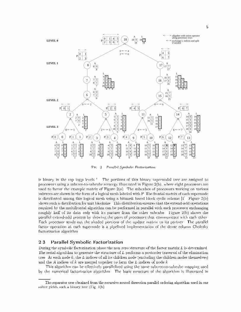
Fig. 3. Parallel Symbolic Factorizationis binary in the top log p levels 1. The portions of this binary supernodal tree are assigned toprocessors using a subtree-to-subcube strategy illustrated in Figure 2(b), where eight processors areused to factor the example matrix of Figure 2(a). The subcubes of processors working on varioussubtrees are shown in the form of a logical mesh labeled with P. The frontal matrix of each supernodeis distributed among this logical mesh using a bitmask based block-cyclic scheme [1]. Figure 2(b)shows such a distribution for unit blocksize. This distribution ensures that the extend-add operationsrequired by the multifrontal algorithm can be performed in parallel with each processor exchangingroughly half of its data only with its partner from the other subcube. Figure 2(b) shows theparallel extend-add process by showing the pairs of processors that communicate with each other.Each processor sends out the shaded portions of the update matrix to its partner. The parallelfactor operation at each supernode is a pipelined implementation of the dense column Choleskyfactorization algorithm.2.3 Parallel Symbolic FactorizationDuring the symbolic factorization phase the non-zero structure of the factor matrix L is determined.The serial algorithm to generate the structure of L performs a postorder traversal of the eliminationtree. At each node k, the L indices of all its children node (excluding the children nodes themselves)and the A indices of k are merged together to form the L indices of node k.This algorithm can be e�ectively parallelized using the same subtree-to-subcube mapping usedby the numerical factorization algorithm. The basic structure of the algorithm is illustrated in1The separator tree obtained from the recursive nested dissection parallel ordering algorithm used in oursolver yields such a binary tree (Fig. 1(b).

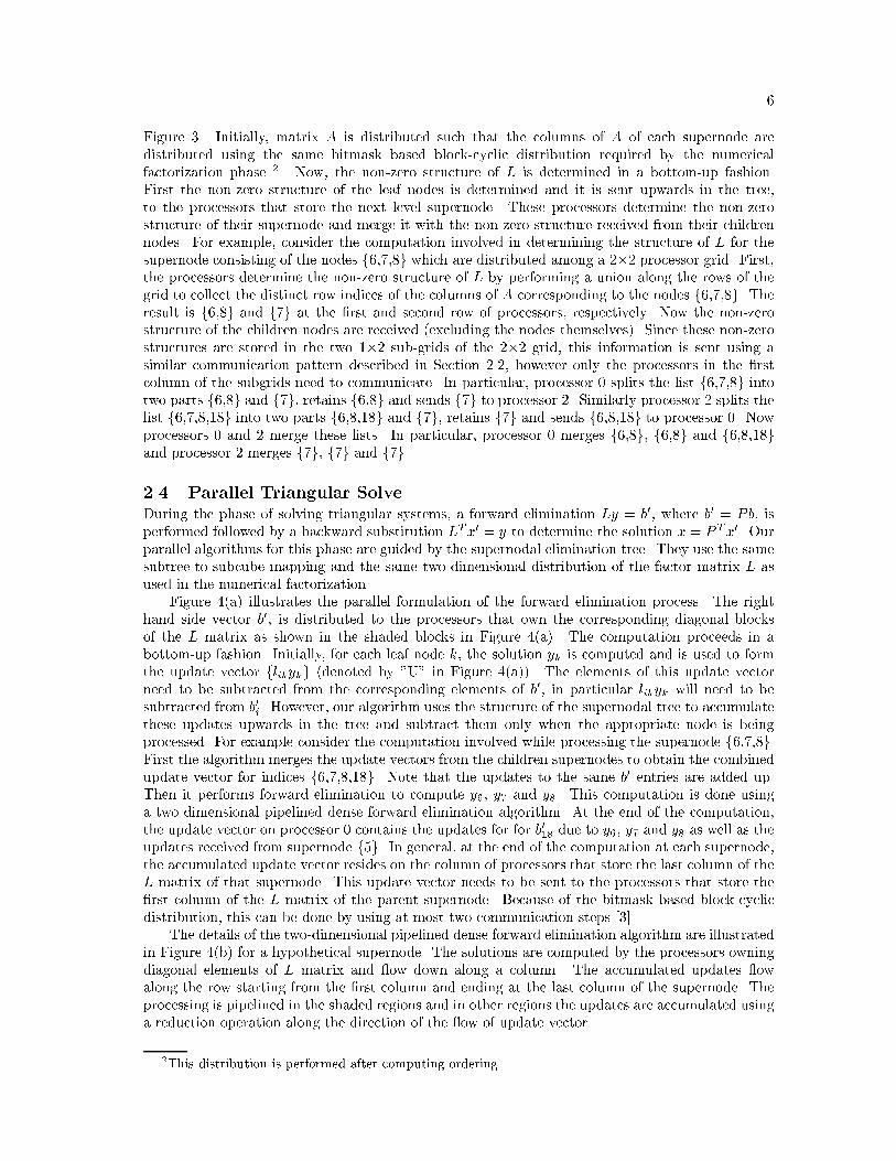
6Figure 3. Initially, matrix A is distributed such that the columns of A of each supernode aredistributed using the same bitmask based block-cyclic distribution required by the numericalfactorization phase 2. Now, the non-zero structure of L is determined in a bottom-up fashion.First the non-zero structure of the leaf nodes is determined and it is sent upwards in the tree,to the processors that store the next level supernode. These processors determine the non-zerostructure of their supernode and merge it with the non-zero structure received from their childrennodes. For example, consider the computation involved in determining the structure of L for thesupernode consisting of the nodes f6,7,8g which are distributed among a 2�2 processor grid. First,the processors determine the non-zero structure of L by performing a union along the rows of thegrid to collect the distinct row indices of the columns of A corresponding to the nodes f6,7,8g. Theresult is f6,8g and f7g at the �rst and second row of processors, respectively. Now the non-zerostructure of the children nodes are received (excluding the nodes themselves). Since these non-zerostructures are stored in the two 1�2 sub-grids of the 2�2 grid, this information is sent using asimilar communication pattern described in Section 2.2, however only the processors in the �rstcolumn of the subgrids need to communicate. In particular, processor 0 splits the list f6,7,8g intotwo parts f6,8g and f7g, retains f6,8g and sends f7g to processor 2. Similarly processor 2 splits thelist f6,7,8,18g into two parts f6,8,18g and f7g, retains f7g and sends f6,8,18g to processor 0. Nowprocessors 0 and 2 merge these lists. In particular, processor 0 merges f6,8g, f6,8g and f6,8,18gand processor 2 merges f7g, f7g and f7g.2.4 Parallel Triangular SolveDuring the phase of solving triangular systems, a forward elimination Ly = b0, where b0 = Pb, isperformed followed by a backward substitution LTx0 = y to determine the solution x = P Tx0. Ourparallel algorithms for this phase are guided by the supernodal elimination tree. They use the samesubtree-to-subcube mapping and the same two-dimensional distribution of the factor matrix L asused in the numerical factorization.Figure 4(a) illustrates the parallel formulation of the forward elimination process. The righthand side vector b0, is distributed to the processors that own the corresponding diagonal blocksof the L matrix as shown in the shaded blocks in Figure 4(a). The computation proceeds in abottom-up fashion. Initially, for each leaf node k, the solution yk is computed and is used to formthe update vector flikykg (denoted by "U" in Figure 4(a)). The elements of this update vectorneed to be subtracted from the corresponding elements of b0, in particular likyk will need to besubtracted from b0i. However, our algorithm uses the structure of the supernodal tree to accumulatethese updates upwards in the tree and subtract them only when the appropriate node is beingprocessed. For example consider the computation involved while processing the supernode f6,7,8g.First the algorithm merges the update vectors from the children supernodes to obtain the combinedupdate vector for indices f6,7,8,18g. Note that the updates to the same b0 entries are added up.Then it performs forward elimination to compute y6, y7 and y8. This computation is done usinga two dimensional pipelined dense forward elimination algorithm. At the end of the computation,the update vector on processor 0 contains the updates for for b018 due to y6, y7 and y8 as well as theupdates received from supernode f5g. In general, at the end of the computation at each supernode,the accumulated update vector resides on the column of processors that store the last column of theL matrix of that supernode. This update vector needs to be sent to the processors that store the�rst column of the L matrix of the parent supernode. Because of the bitmask based block-cyclicdistribution, this can be done by using at most two communication steps [3].The details of the two-dimensional pipelined dense forward elimination algorithm are illustratedin Figure 4(b) for a hypothetical supernode. The solutions are computed by the processors owningdiagonal elements of L matrix and ow down along a column. The accumulated updates owalong the row starting from the �rst column and ending at the last column of the supernode. Theprocessing is pipelined in the shaded regions and in other regions the updates are accumulated usinga reduction operation along the direction of the ow of update vector.2This distribution is performed after computing ordering.

7

0

00

20

76

2

L

855

11

511151617

L

4

65

18

3

5

334

101115

35555

10

12141718

66666666

12

358

16

22223

1267 18

11111

0

78

20000

13141518

777713

9111617

4444

9

01818

L

33

33

5678

185

L

1

1

3

3

1

U

pipelined processing

all-to-one gather operation

22

0

3

576

73

8

7

6

2

3 4 9 12 13

16

17

15

18

5 11 14

1010

L L LLLL L L

02 3

10 00 01

678

186 7 8

L

575

4

46 7

5

15161718

15 16 17

L

0

00

678

3333

678

18

555

151617

111

222

333

444

555

666

777

000

267

58

1865

18

111617

111516

141718

78

2 141518

0

U UU

U U U U U U UU

U U

018 518

0 1 3 4 5 6

0 35

0

2

0

2

0

2

0

2

0 1

3

1

3

1

3

1

3

0

2

0

2

0

2

0 1

3

1

3

1

3

(b)

2

7

7

7 2

32 54 6701

update flow

solutionflow

(a)

0

and the computed solution for index kprocessor p is assigned to the right-hand side:

kpk

L

L : Columns of Lower Triangular Cholesky Factor

U : Update vector accumulated upwards in the tree05

6666

15161718

UL

6666

15161718

14

14

6

Fig. 4. Parallel Triangular Solve. (a). Entire process of parallel forward elimination for the examplematrix. (b). Processing within a hypothetical supernodal matrix for forward elimination.The algorithm for parallel backward substitution is similar, except for two di�erences. First, thecomputation proceeds from the top supernode of the tree down to the leaf. Second, the computedsolution that gets communicated across the levels of the supernodal tree instead of accumulatedupdates and this is achieved with at most one communication per processor. Refer to [3] for details.2.5 Parallel Runtime and Scalability AnalysisAnalyzing a general sparse solver is a di�cult problem. We present the analysis for two wide classesof sparse systems arising out of two-dimensional and three-dimensional constant node-degree graphs.We refer to these problems as 2-D and 3-D problems, respectively.Let a problem of dimension N be solved using p processors. De�ne l as a level in the supernodaltree with l = 0 for the topmost level. Thus, the number of processors assigned to a level l supernodeis p=2l. With a nested dissection based ordering scheme, it has been shown that the average size ofa frontal matrix at level l is �(N=22l) for 2-D problems, and �(N4=3=24l) for 3-D problems. Also,the number of nodes in a level-l supernode is on an average �(pN=2l) and �((N=2l)2=3) for 2-D and3-D problems, respectively. The number of non-zeros in L is N logN for 2-D problems, and N4=3for 3-D problems. Using this information, the parallel algorithms presented earlier in this sectionhave been analyzed for their parallel runtime. For details, refer to [2, 3].Table 1 shows the serial runtime complexity, parallel overhead, and isoe�ciency functions [7]for all four phases. It can be seen that all the phases are scalable to varying degrees. Since theoverall time complexity is dominated by the numerical factorization phase, the isoe�ciency functionof the entire parallel solver is determined by the numerical factorization phase, and it is O(p1:5) forboth 2-D and 3-D problems. As discussed in [7], the isoe�ciency function of the dense Choleskyfactorization algorithm is also O(p1:5). Thus our sparse direct solver is as scalable as the densefactorization algorithm.

82-D constant node-degree graph 3-D constant node-degree graphPhase Ts To IsoE� Ts To IsoE�Order O(N logN) O(p2 log p) O(p2 log p) O(N logN) O(p2 log p) O(p2 log p)SymFact O(N logN) O(pNp log p) O(p log p) O(N4=3) O(N2=3pp) O(p)NumFact O(N3=2) O(Npp) O(ppp) O(N2) O(N4=3pp) O(ppp)TriSolve O(N logN) O(pNp) O(p2= log p) O(N4=3) O(N2=3p) O(p2)Table 1Complexity Analysis of various phases of our parallel solver for N-vertex constant node-degree graphs.Notations: Ts = Serial Runtime Complexity, To = Parallel Overhead = pTp � Ts, where Tp is the ParallelRuntime. IsoE� is the isoe�ciency function indicating the rate at which the problem size should increasewith the number of processors to achieve same e�ciency.3 Library Implementation and Experimental ResultsWe have implemented all the parallel algorithms presented in previous section, and integrated theminto a library called PSPASES [4]. This library uses MPI call interface for communication, andBLAS interface for computation within a processor. This makes PSPASES portable to a widerange of parallel computers. Furthermore, using BLAS, it is able to achieve high computationalperformance especially on the platforms with vendor-tuned BLAS libraries.We have incorporated some more features into PSPASES to make it easy-to-use. The libraryprovides simple functional interfaces, and allows user to call its functions from both C and Fortran90 programs. It uses the concept of a communicator which relieves the user from managing thememory required by various internal data structures. The communicator also allows to solve multiplesystems with same sparsity structure, or same system for multiple sets of right hand side matrix,B. PSPASES also provides the user with useful statistical information such as the load imbalanceof the supernodal elimination tree, number of �ll-ins (both of which can be used to judge thequality of ordering), operation count for factor operation, and estimation of memory for internaldata structures.We have tested PSPASES on a wide range of parallel machines, for a wide range of sparsematrices. Tables 3 and 4 give experimental results obtained on a 32-processor SGI Origin 2000 anda 256-processor Cray T3E-1200, respectively. We used native versions of both the MPI and BLASlibraries. The notations used in presenting the results are described in Table 2. We give numbersfor the numerical factorization and triangular solve phases only. The parallel ordering algorithm weuse is incorporated into a separate library called ParMetis [6], and PSPASES library functions justcall the ParMetis library functions. ParMetis performance numbers are reported elsewhere [6]. Thesymbolic factorization took relatively very small time, and hence, we do not report those numbershere.It should be noted that the blocksize of distributing supernodal matrices and the load balanceof the supernodal tree played important roles in determining the performance of the solver. Also,since most of today's parallel computers have better communication performance for larger databeing communicated, blocksize optimal for numerical factorization need not be optimal for triangularsolve phase, which has relatively small data communication per computational block. For the resultspresented, blocks of 1024 or 4096 double precision numbers worked best for numerical factorizationphase.It can be seen from Tables 3 and 4, that numerical factorization phase demonstrates highperformance and scalability for all the matrices. Triangular solve phase also yields a very highperformance, but for larger number of processors it tends to show an unscalable behavior. Wepro�led various parts of the code to see where the unscalability was appearing and found that itwas in the part where b and x0 are being permuted in parallel (b0 = Pb and x = P Tx0). Analyzingit further showed that bad performance of all-to-all operations of underlying MPI library for largechunks of data being exchanged among large number of processors caused such a behavior. Thebasic algorithms for both forward elimination and backward substitution performed scalably.

9N : Dimension of A.NNZ LowerA : Number of non-zeros in Lower triangular part of A (including diagonal).np : Number of Processors.NNZ L : Number of non-zeros in L.Imbal : Computational Load Imbalance due to supernodal tree structure.FAC OPC : Operation count for Numerical Factor phase.Ntime : Numerical Factor Time (in seconds).Nperf : Numerical Factor Performance (in MFLOPS).Ttime : Redistribution of b and x + Triangular Solve Time for nrhs = 1.Table 2Notations used in the presented resultsThe highest performance of 51 GFLOPS was obtained for numerical factorization for the 1-million equation system CUBE100, on 256 processors of Cray T3E-1200. To our knowledge, thisis the largest sparse system ever solved by a direct solution method, with the highest performanceever reported.We have made PSPASES library and more experimental results available via WWW at URL:http://www.cs.umn.edu/~mjoshi/pspases.References[1] Anshul Gupta, George Karypis and Vipin Kumar, Highly Scalable Parallel Algorithms for SparseMatrix Factorization, IEEE Transactions on Parallel and Distributed Systems, vol. 8, no. 5, pp. 502-520, 1997.[2] Anshul Gupta, Analysis and Design of Scalable Parallel Algorithms for Scienti�c Computing, Ph.D.Thesis, Department of Computer Science, University of Minnesota, Minneapolis, 1995.[3] Mahesh Joshi, Anshul Gupta, George Karypis and Vipin Kumar, A High Performance Two Dimen-sional Scalable Parallel Algorithm for Solving Sparse Triangular Systems, Proc. of 4th Int. Conf. onHigh Performance Computing (HiPC'97), Bangalore, India, 1997.[4] Mahesh Joshi, George Karypis, Vipin Kumar, Anshul Gupta, and Fred Gustavson, PSPASES: ScalableParallel Direct Solver Library for Sparse Symmetric Positive De�nite Linear Systems (Version 1.0),User's Manual, Available via http://www.cs.umn.edu/~mjoshi/pspases.[5] George Karypis and Vipin Kumar, Parallel Algorithm for Multilevel Graph Partitioning and SparseMatrix Ordering, Journal of Parallel and Distributed Computing, vol. 48, pp. 71-95, 1998.[6] George Karypis, Kirk Schlogel, and Vipin Kumar ParMetis: Parallel Graph Partitioning and SparseMatrix Ordering Library, (Version 1.0), User's Manual, Available via http://www.cs.umn.edu/~metis.[7] Vipin Kumar, Ananth Grama, Anshul Gupta and George Karypis, Introduction to Parallel Computing:Design and Analysis of Algorithms Benjamin/Cummings, Redwood City, CA, 1994.[8] Joseph W. H. Liu, The Multifrontal Method for Sparse Matrix Solution: Theory and Practice, SIAMReview, vol. 34, no.1, pp. 82-109, March 1992.[9] Joseph W. H. Liu, The Role of Elimination Trees in Sparse Factorization, SIAM Journal of MatrixAnalysis and Applications, vol. 11, pp. 134-172, 1990.

10np NNZ L Imbal FAC OPC Ntime Nperf Ttimematrix : MDUAL2, N: 988605, NNZ LowerA: 2.9357E+064 1.77e+8 1.29 3.20e+11 685.420 466.56 8.8998 1.90e+8 1.66 3.98e+11 490.000 811.57 5.15116 1.96e+8 1.32 4.09e+11 256.588 1592.17 3.21732 1.92e+8 1.43 3.63e+11 140.110 2590.74 2.399matrix : AORTA, N: 577771, NNZ LowerA: 1.7067E+064 7.64e+7 1.48 7.95e+10 163.648 485.87 4.4758 7.79e+7 1.74 8.47e+10 92.727 913.89 2.56616 8.20e+7 2.59 9.46e+10 79.850 1185.14 1.63332 8.49e+7 2.46 1.02e+11 52.877 1936.23 1.314matrix : CUBE65, N: 274625, NNZ LowerA: 1.0858E+064 1.33e+8 1.11 4.04e+11 737.626 547.68 4.8788 1.32e+8 1.15 4.04e+11 485.296 832.73 2.55016 1.36e+8 1.27 4.19e+11 306.904 1363.67 1.42332 1.40e+8 1.27 4.27e+11 137.730 3100.99 1.379matrix : S3DKQ4M2, N: 90449, NNZ LowerA: 2.4600E+062 1.90e+7 1.05 8.87e+09 22.418 395.49 0.9464 1.92e+7 1.10 8.72e+09 12.351 705.93 0.5708 2.17e+7 1.44 1.29e+10 12.249 1051.67 0.58316 2.18e+7 1.43 1.25e+10 7.357 1702.44 0.61332 2.29e+7 1.58 1.36e+10 6.404 2124.37 0.596matrix : COPTER2, N: 55476, NNZ LowerA: 4.0771E+052 9.88e+6 1.01 5.84e+09 14.433 404.61 0.6244 1.02e+7 1.08 6.47e+09 9.102 710.73 0.4388 1.06e+7 1.50 6.85e+09 6.960 984.09 0.39716 1.11e+7 1.39 7.38e+09 4.616 1599.81 0.38032 1.19e+7 1.39 8.29e+09 4.121 2011.69 0.422matrix : BCSSTK18, N: 11948, NNZ LowerA: 8.0500E+042 6.18e+5 1.35 1.01e+08 0.672 149.58 0.0844 6.54e+5 1.88 1.17e+08 0.496 234.91 0.0518 6.71e+5 1.47 1.21e+08 0.272 444.55 0.03416 8.10e+5 2.30 1.82e+08 0.302 602.09 0.03432 7.56e+5 1.95 1.45e+08 0.270 537.83 0.051Table 3Performance for factorization and solve phases on SGI Origin 2000

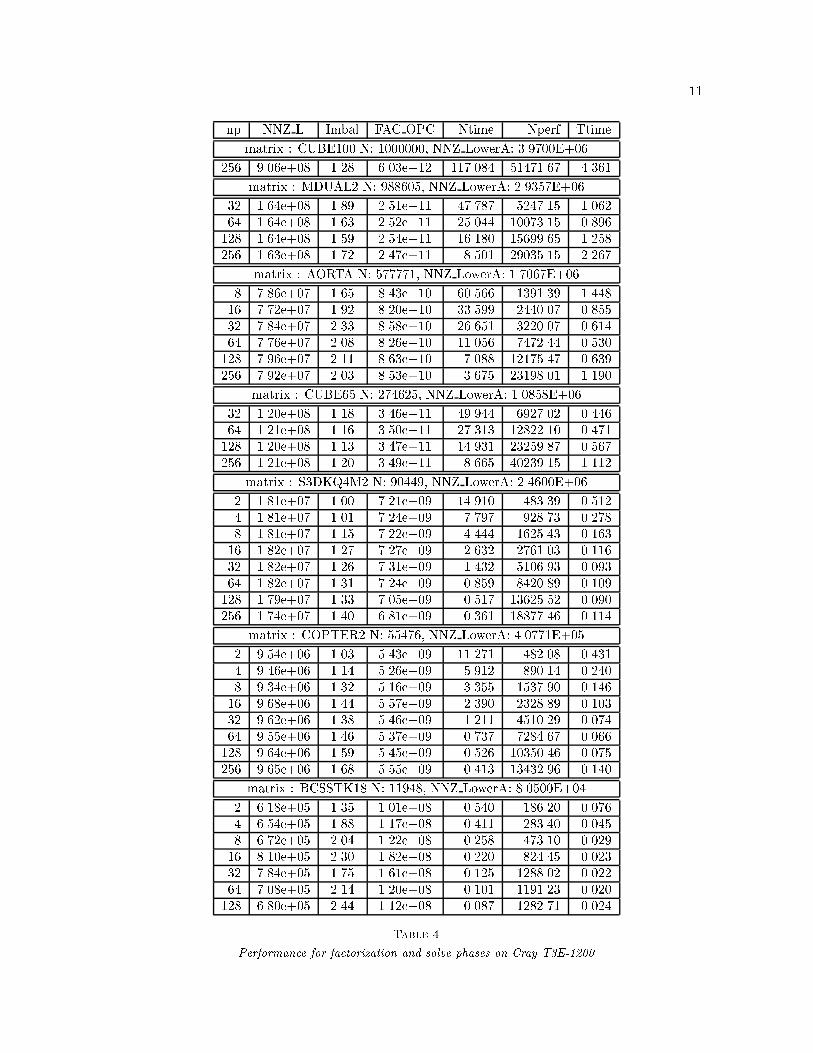
11np NNZ L Imbal FAC OPC Ntime Nperf Ttimematrix : CUBE100 N: 1000000, NNZ LowerA: 3.9700E+06256 9.06e+08 1.28 6.03e+12 117.084 51471.67 4.361matrix : MDUAL2 N: 988605, NNZ LowerA: 2.9357E+0632 1.64e+08 1.89 2.51e+11 47.787 5247.15 1.06264 1.64e+08 1.63 2.52e+11 25.044 10073.15 0.896128 1.64e+08 1.59 2.54e+11 16.180 15699.65 1.258256 1.63e+08 1.72 2.47e+11 8.501 29035.15 2.267matrix : AORTA N: 577771, NNZ LowerA: 1.7067E+068 7.86e+07 1.65 8.43e+10 60.566 1391.39 1.44816 7.72e+07 1.92 8.20e+10 33.599 2440.07 0.85532 7.84e+07 2.33 8.58e+10 26.651 3220.07 0.61464 7.76e+07 2.08 8.26e+10 11.056 7472.44 0.530128 7.96e+07 2.11 8.63e+10 7.088 12175.47 0.639256 7.92e+07 2.03 8.53e+10 3.675 23198.01 1.190matrix : CUBE65 N: 274625, NNZ LowerA: 1.0858E+0632 1.20e+08 1.18 3.46e+11 49.944 6927.02 0.44664 1.21e+08 1.16 3.50e+11 27.313 12822.10 0.471128 1.20e+08 1.13 3.47e+11 14.931 23259.87 0.567256 1.21e+08 1.20 3.49e+11 8.665 40239.15 1.112matrix : S3DKQ4M2 N: 90449, NNZ LowerA: 2.4600E+062 1.81e+07 1.00 7.21e+09 14.910 483.39 0.5124 1.81e+07 1.01 7.24e+09 7.797 928.73 0.2788 1.81e+07 1.15 7.22e+09 4.444 1625.43 0.16316 1.82e+07 1.27 7.27e+09 2.632 2761.03 0.11632 1.82e+07 1.26 7.31e+09 1.432 5106.93 0.09364 1.82e+07 1.31 7.24e+09 0.859 8420.89 0.109128 1.79e+07 1.33 7.05e+09 0.517 13625.52 0.090256 1.74e+07 1.40 6.81e+09 0.361 18877.46 0.114matrix : COPTER2 N: 55476, NNZ LowerA: 4.0771E+052 9.54e+06 1.03 5.43e+09 11.271 482.08 0.4314 9.46e+06 1.14 5.26e+09 5.912 890.14 0.2408 9.34e+06 1.32 5.16e+09 3.355 1537.90 0.14616 9.68e+06 1.44 5.57e+09 2.390 2328.89 0.10332 9.62e+06 1.38 5.46e+09 1.211 4510.29 0.07464 9.55e+06 1.46 5.37e+09 0.737 7284.67 0.066128 9.64e+06 1.59 5.45e+09 0.526 10350.46 0.075256 9.65e+06 1.68 5.55e+09 0.413 13432.96 0.140matrix : BCSSTK18 N: 11948, NNZ LowerA: 8.0500E+042 6.18e+05 1.35 1.01e+08 0.540 186.20 0.0764 6.54e+05 1.88 1.17e+08 0.411 283.40 0.0458 6.72e+05 2.04 1.22e+08 0.258 473.10 0.02916 8.10e+05 2.30 1.82e+08 0.220 824.45 0.02332 7.84e+05 1.75 1.61e+08 0.125 1288.02 0.02264 7.08e+05 2.14 1.20e+08 0.101 1191.23 0.020128 6.80e+05 2.44 1.12e+08 0.087 1282.71 0.024Table 4Performance for factorization and solve phases on Cray T3E-1200