ON THE GLOBAL SOLUTION OF LINEAR PROGRAMS WITH LINEARCOMPLEMENTARITY CONSTRAINTS∗

JING HU, JOHN E. MITCHELL, JONG-SHI PANG, KRISTIN P. BENNETT, AND GAUTAM KUNAPULI

Abstract. This paper presents a parameter-free integer-programming based algorithm for the global resolution of a linear programwith linear complementarity constraints (LPCC). The cornerstone of the algorithm is a minimax integer program formulation thatcharacterizes and provides certificates for the three outcomes—infeasibility, unboundedness, or solvability—of an LPCC. An extremepoint/ray generation scheme in the spirit of Benders decomposition is developed, from which valid inequalities in the form of satisfiabilityconstraints are obtained. The feasibility problem of these inequalities and the carefully guided linear programming relaxations of theLPCC are the workhorse of the algorithm, which also employs a specialized procedure for the sparsification of the satifiability cuts. Weestablish the finite termination of the algorithm and report computational results using the algorithm for solving randomly generatedLPCCs of reasonable sizes. The results establish that the algorithm can handle infeasible, unbounded, and solvable LPCCs effectively.

1. Introduction. Forming a subclass of the class of mathematical programs with equilibrium/complementarityconstraints (MPECs/MPCCs) [37, 39, 12], linear programs with linear complementarity constraints (LPCCs) aredisjunctive linear optimization problems that contain a set of complementarity conditions. In turn, a large sub-class of LPCCs are bilevel linear/quadratic programs [11] that provide a broad modeling framework for parameteridentification in convex quadratic programming; an example of such an application was proposed recently for thecross validation of a host of machine learning problems [6, 33, 32]. While there have been significant recent ad-vances on nonlinear programming (NLP) based computational methods for solving MPECs and the closely relatedMPCCs, [1, 2, 3, 8, 15, 16, 19, 20, 29, 30, 25, 35, 36, 44, 45], much of which have nevertheless focused on obtain-ing stationary solutions [13, 14, 37, 39, 38, 40, 44, 50, 49, 48], the global solution of an LPCC remains elusive.Particularly impressive among these advances is the suite of NLP solvers publicly available on the neos systemat http://www-neos.mcs.anl.gov/neos/solvers/index.html; many of them, such as filter and knitro, arecapable of producing a solution of some sort to an LPCC very efficiently. Yet, they are incapable of ascertainingthe quality of the computed solution. This is the major deficiency of these numerical solvers. Continuing our forayinto the subject of computing global solutions of LPCCs, which begins with the recent article [42] that pertains toa special problem arising from the optimization of the value-at-risk, the present paper proposes a parameter-freeinteger-programming based cutting-plane algorithm for globally resolving a general LPCC.

As a disjunctive linear optimization problem, the global solution of an LPCC has been the subject of sustained,but not particularly focused investigation since the early work of Ibaraki [26, 27] and Jeroslow [28], who pioneeredsome cutting-plane methods for solving a “complementary program”, which is a historical and not widely usedname for an LPCC. Over the years, various integer programming based methods [4, 5, 21] and global optimizationbased methods [17, 18, 46, 47] have been developed that are applicable to an LPCC. In this paper, we present a newcutting-plane method that will successfully resolve a general LPCC in finite time; i.e., the method will terminatewith one of the following three mutually exclusive conclusions: the LPCC is infeasible, the LPCC is feasible but hasan unbounded objective, or the LPCC attains a finite optimal solution. We also leverage the advances of the NLPsolvers and use two of them to benchmark our algorithm. In addition, we propose a simple linear programmingbased pre-processor whose effectiveness will be demonstrated via computational results.

The proposed method begins with an equivalent formulation of an LPCC as a 0-1 integer program (IP) involvinga conceptually very large parameter, whose existence is not guaranteed unless a certain boundedness condition holds.Via dualization of the linear programming relaxation of the IP, we obtain a minimax 0-1 integer program, whichyields a certificate for the three states of the LPCC, without any a priori boundedness assumption. The original0-1 IP with the conceptual parameter provides the formulation for the application of Benders decomposition [34],which we show can be implemented without involving the parameter in any way. Thus, the resulting algorithm isreminiscent of the well-known Phase I implementation of the “big-M” method for solving linear programs, whereinthe big-M formulation is only conceptual whose practical solution does not require the knowledge of the scalar M.

The implementation of our parameter-free algorithm is accomplished by solving integer subprograms definedsolely by satisfiability constraints [7, 31]; in turn, each such constraint corresponds to a “piece” of the LPCC.Using this interpretation, the overall algorithm can be considered as solving the LPCC by searching on its (finitely

∗This work was supported in part by the Office of Naval Research under grant no. N00014-06-1-0014. The work of Mitchell wassupported by the National Science Foundation under grant DMS-0317323. All authors, except Pang, are affiliated with the Departmentof Mathematical Sciences, Rensselaer Polytechnic Institute, Troy, New York 12180-1590, U.S.A. Their email addresses are: huj, mitchj,bennek, kunapg@rpi.edu, respectively. Pang was affiliated with the same department when the original manuscript was written; he ispresently affiliated with the Department of Industrial and Enterprise Systems Engineering, University of Illinois at Urbana-Champaign,Urbana, Illinois 61801, U.S.A. Pang’s email address is: jspang@uiuc.edu.

1

many) linear programming pieces, with the search guided by solving the satisfiability IPs. The implementation ofthe algorithm is aided by valid upper bounds on the LPCC optimal objective value that are being updated as thealgorithm progresses, which also serve to provide the desired certificates at the termination of the algorithm.

Hooker [22, 23] and Hooker and Ottosson [24] have presented a general Benders decomposition framework forinteger programming problems, where the subproblems and the master problem may be solved by various tech-niques, for example constraint programming. The constraints returned by the subproblems may well be satisfiabilityconstraints similar to those we derive from solving a linear programming subproblem, leading to a satisfiabilitymaster problem. Hooker develops a broad framework for integrating different solution methodologies, with thesolution approaches driven by the types of constraints. Different decomposition methods are available dependingon the particular mix of types of constraints. Codato and Fischetti [9] have specialized Hooker’s approach tosolve integer programs arising from linear programs with conditional constraints of the kind “if then”, of whichthe complementarity condition is a special case. Such constraints are modeled with the introduction of integervariables together with a big-M coefficients. The cited article presents computational results for feasible boundedproblems where only the binary variables associated with the big-M coefficients appear in the objective function.In our problem (2.3), the objective function is a linear function of the continuous variables; the objective functioncould be regarded as a nonlinear function of the binary variables (see ϕ(z) defined in (2.9)). Our algorithmicapproach can successfully characterize infeasible and unbounded LPCC problems as well as solve problems withfinite optimal value. Hooker [23] states that “the success of a Benders method often rests on finding strong Benderscuts that rule out as many infeasible solutions as possible”. The sparsification methodology we present in Section 4is an approach to generate strong Benders cuts.

The organization of the rest of the paper is as follows. Section 2 presents the formal statement of the LPCC,summarizes the three states of the LPCC, and introduces the new minmax IP formulation. Section 3 reformulatesthe minmax IP formulation in terms of the extreme points and rays of the key polyhedron Ξ (see (2.6)) andestablished the theoretical foundation for the cutting-plane algorithm to be presented in Section 5. The keysteps of the algorithm, which involve solving linear programs (LPs) to sparsify the satisfiability constraints, areexplained in Section 4. The sixth and last section reports the computational results and completes the paper withsome concluding remarks.

2. Preliminary Discussion. Let c ∈ <n, d ∈ <m, f ∈ <k, q ∈ <m, A ∈ <k×n, B ∈ <k×m, M ∈ <m×m, andN ∈ <m×n be given. Consider the linear program with linear complementarity constraints (LPCC) [41] of finding(x, y) ∈ <n ×<m in order to

minimize(x,y)

cTx+ dT y

subject to Ax+By ≥ f

and 0 ≤ y ⊥ q +Nx+My ≥ 0,

(2.1)

where a ⊥ b means that the two vectors are orthogonal; i.e., aT b = 0. It is well-known that the LPCC is equivalentto the minimization of a large number of linear programs, each defined on one piece of the feasible region of theLPCC. That is, for each subset α of {1, · · · ,m} with complement α, we may consider the LP(α):

minimize(x,y)

cTx+ dT y

subject to Ax+By ≥ f

( q +Nx+My )α ≥ 0 = yα

and ( q +Nx+My )α = 0 ≤ yα.

(2.2)

The following facts are consequences of the disjunctive property of the complementarity condition:(a) the LPCC (2.1) is infeasible if and only if the LP(α) is infeasible for all α ⊆ {1, · · · ,m};(b) the LPCC (2.1) is feasible and has an unbounded objective if and only if the LP(α) is feasible and has an

unbounded objective for some α ⊆ {1, · · · ,m};(c) the LPCC (2.1) is feasible and attains a finite optimal objective value if and only if (i) a subset α of {1, · · · ,m}

exists such that the LP(α) is feasible, and (b) every such feasible LP(α) has a finite optimal objectivevalue; in this case, the optimal objective value of the LPCC (2.1), denoted LPCCmin, is the minimum ofthe optimal objective values of all such feasible LPs.

The first step in our development of an IP-based algorithm for solving the LPCC (2.1) without any a prioriassumption is to derive results parallel to the above three facts in terms of some parameter-free integer problems.

2

For this purpose, we recall the standard approach of solving (2.1) as an IP containing a large parameter. Thisapproach is based on the following “equivalent” IP formulation of (2.1) wherein the complementarity constraint isreformulated in terms of the binary vector z ∈ {0, 1}m via a conceptually very large scalar θ > 0:

minimize(x,y,z)

cTx+ dT y

subject to Ax+By ≥ f

θ z ≥ q +Nx+My ≥ 0

θ( 1− z ) ≥ y ≥ 0

and z ∈ { 0, 1 }m,

(2.3)

where 1 is the m-vector of all ones. In the standard approach, we first derive a valid value on θ by solving LPs toobtain bounds on all the variables and constraints of (2.1). We then solve the fixed IP (2.3) using the so-obtainedθ by, for example, the Benders approach. There are two drawbacks of such an approach: one is the limitationof the approach to problems with bounded feasible regions; the other drawback is the nontrivial computation toderive the required bounds even if they are known to exist implicitly. In contrast, our new approach removes sucha theoretical restriction and eliminates the front-end computation of bounds. The price of the new approach isthat it solves a (finite) family of IPs of a special type, each defined solely by constraints of the satisfiability type.The following discussion sets the stage for the approach. [A referee suggests that “another drawback of attackingthe integer program (2.3) is the probably (very) weak LP relaxations (which will affect the convergence of branchand cut methods as well as approaches based on Benders decomposition)”.]

For a given binary vector z and a positive scalar θ, we associate with (2.3) the linear program below, which wedenote LP(θ; z):

minimize(x,y)

cTx+ dT y

subject to Ax+By ≥ f (λ )

Nx+My ≥ −q (u− )

−Nx−My ≥ q − θ z (u+ )

−y ≥ −θ ( 1− z ) ( v )

and y ≥ 0,

(2.4)

where the dual variables of the respective constraints are given in the parentheses. The dual of (2.4), which wedenote DLP(θ, z), is:

maximize(λ,u±,v)

fTλ+ qT (u+ − u− )− θ[zTu+ + ( 1− z )T v

]subject to ATλ−NT (u+ − u− ) = c

BTλ−MT (u+ − u− )− v ≤ d

and (λ, u±, v ) ≥ 0.

(2.5)

Let Ξ ⊆ <k+3m be the feasible region of the DLP(θ, z); i.e.,

Ξ ≡

{(λ, u±, v ) ≥ 0 : ATλ−NT (u+ − u− ) = c

BTλ−MT (u+ − u− )− v ≤ d

}. (2.6)

Note that Ξ is a fixed polyhedron independent of the pair (θ, z); Ξ has at least one extreme point if it is nonempty.Let LPmin(θ; z) and d(θ; z) denote the optimal objective value of (2.4) and (2.5), respectively. Throughout, we adoptthe standard convention that the optimal objective value of an infeasible maximization (minimization) problemis defined to be −∞ (∞, respectively). We summarize some basic relations between the above programs in thefollowing result.

Proposition 2.1. The following three statements hold.3

(a) Any feasible solution (x0, y0) of (2.1) induces a pair (θ0, z0), where θ0 > 0 and z0 ∈ {0, 1}m, such that the

tuple (x0, y0, z0) is feasible to (2.3) for all θ ≥ θ0; such a z0 has the property that

( q +Nx0 +My0 )i > 0 ⇒ z0i = 1

( y0 )i > 0 ⇒ z0i = 0.

(2.7)

(b) Conversely, if (x0, y0, z0) is feasible to (2.3) for some θ ≥ 0, then (x0, y0) is feasible to (2.1).(c) If (x0, y0) is an optimal solution to (2.1), then it is optimal to the LP(θ, z0) for all pairs (θ, z0) such that θ ≥ θ0

and z0 satisfies (2.7); moreover, for each θ > θ0, any optimal solution (λ, u±, v) of the DLP(θ, z0) satisfies(z0)T u+ + ( 1− z0 )T v = 0.

Proof. Only (c) requires a proof. Suppose (x0, y0) is optimal to (2.1). Let (θ, z0) such that θ ≥ θ0 and z0 ∈ {0, 1}msatisfies (2.7). Then (x0, y0) is feasible to the LP(θ, z0); hence

cTx0 + dT y0 ≥ LPmin(θ, z0). (2.8)

But the reverse inequality must hold because of (b) and the optimality of (x0, y0) to (2.1). Consequently, equalityholds in (2.8). For θ > θ0, if i is such that z0

i > 0, then

( q +Nx0 +My0 ) ≤ θ0 z0i < θ z0

i ,

and complementary slackness implies (u+)i = 0. Similarly, we can show that z0i = 0 ⇒ vi = 0. Hence (c) follows.

�

2.1. The parameter-free dual programs. Property (c) of Proposition 2.1 suggests that the inequalityconstraint zTu+ + (1 − z)T v ≤ 0, or equivalently, the equality constraint zTu+ + (1 − z)T v = 0 (because allvariables are nonnegative and z ∈ {0, 1}m), should have an important role to play in an IP approach to the LPCC.This motivates us to define two value functions on the binary vectors. Specifically, for any z ∈ {0, 1}m, define

< ∪ {±∞} 3 ϕ(z) ≡ maximum(λ,u±,v)

fTλ+ qT (u+ − u− )

subject to ATλ−NT (u+ − u− ) = c

BTλ−MT (u+ − u− )− v ≤ d

(λ, u±, v ) ≥ 0

and zTu+ + (1− z)T v ≤ 0

(2.9)

and its homogenization:

{ 0,∞} 3 ϕ0(z) ≡ maximum(λ,u±,v)

fTλ+ qT (u+ − u− )

subject to ATλ−NT (u+ − u− ) = 0

BTλ−MT (u+ − u− )− v ≤ 0

(λ, u±, v ) ≥ 0

and zTu+ + ( 1− z )T v ≤ 0.

(2.10)

Clearly, (2.10) is always feasible and ϕ0(z) takes on the values 0 or ∞ only. Unlike (2.10) which is independent ofthe pair (c, d), (2.9) depends on (c, d) and is not guaranteed to be feasible; thus ϕ(z) ∈ < ∪ {±∞}. For any pair(c, d) for which (2.9) is feasible, we have

ϕ(z) < ∞ ⇔ ϕ0(z) = 0.

To this equivalence we add the following proposition that describes a one-to-one correspondence between (2.10)and the feasible pieces of the LPCC. The support of a vector z, denoted supp(z) is the index set of the nonzerocomponents of z.

Proposition 2.2. For any z ∈ {0, 1}m, ϕ0(z) = 0 if and only if the LP(α) is feasible, where α ≡ supp(z).4

Proof. The dual of (2.10) is

minimize(x,y)

0Tx+ 0T y

subject to Ax+By ≥ f

θ z ≥ q +Nx+My ≥ 0

and θ ( 1− z ) ≥ y ≥ 0.

(2.11)

By LP duality, it follows that if ϕ0(z) = 0, then (2.11) is feasible for any θ > 0; conversely, if (2.11) is feasiblefor some θ > 0, then ϕ0(z) = 0. In turn, (2.11) is feasible for some θ > 0 if and only if the LP(α) is feasible forα ≡ supp(z). �

For subsequent purposes, it would be useful to record the following equivalence between the extreme points/raysof the feasible region of (2.9) and those of the feasible set Ξ.

Proposition 2.3. For any z ∈ [0, 1]m, a feasible solution (λp, u±,p, vp) of (2.9) is an extreme point in thisregion if and only if it is extreme in Ξ; a feasible ray (λr, u±,r, vr) of (2.9) is extreme in this region if and only ifit is extreme in Ξ.Proof. We prove only the first assertion; that for the second is similar. The sufficiency holds because the feasibleregion of (2.9) is a subset of Ξ. To prove the converse, suppose that (λp, u±,p, vp) is an extreme solution of (2.9).Then this triple must be an element of Ξ. If it lies on the line segment of two other feasible solutions of Ξ, thenthe latter two solutions must satisfy the additional constraint zTu+ + (1 − z)T v ≤ 0. Therefore, (λp, u±,p, vp) isalso extreme in Ξ. �

2.2. The set Z and a minimax formulation. We now define the key set of binary vectors:

Z ≡ { z ∈ { 0, 1 }m : ϕ0(z) = 0 } ,

which, by Proposition 2.2, is the feasibility descriptor of the feasible region of the LPCC (2.1). Note that Z is afinite set. We also define the minimax integer program:

minimizez∈Z

ϕ(z) ≡

maximum(λ,u±,v)

fTλ+ qT (u+ − u− )

subject to ATλ−NT (u+ − u− ) = c

BTλ−MT (u+ − u− )− v ≤ d

(λ, u±, v ) ≥ 0

and zTu+ + (1− z)T v ≤ 0.

(2.12)

Since Z is a finite set, and since ϕ(z) ∈ < ∪ {−∞} for z ∈ Z, it follows that argminz∈Z

ϕ(z) 6= ∅ if and only if Z 6= ∅.

The following result rephrases the three basic facts connecting the LPCC (2.1) and its LP pieces in terms of theIP (2.12).

Theorem 2.4. The following three statements hold:(a) the LPCC (2.1) is infeasible if and only if min

z∈Zϕ(z) =∞ (i.e., Z = ∅);

(b) the LPCC (2.1) is feasible and has an unbounded objective value if and only if minz∈Z

ϕ(z) = −∞ (i.e., z ∈ Zexists such that ϕ(z) = −∞);

(c) the LPCC (2.1) attains a finite optimal objective value if and only if −∞ < minz∈Z

ϕ(z) <∞.

In all cases, LPCCmin = minz∈Z

ϕ(z); moreover, for any z ∈ {0, 1}m for which ϕ(z) > −∞, LPCCmin ≤ ϕ(z).

Proof. Statement (a) is an immediate consequence of Proposition 2.2. Statement (b) is equivalent to saying thatthe LPCC (2.1) is feasible and has an unbounded objective if and only if z ∈ {0, 1}m exists such that ϕ0(z) = 0and ϕ(z) = −∞. Suppose that the LPCC (2.1) is feasible and unbounded. Then an index set α ⊆ {1, · · · ,m}exists such that the LP(α) is feasible and unbounded. Letting z ∈ {0, 1}m be such that supp(z) = α and α be the

5

complement of α in {1, · · · ,m}, we have ϕ0(z) = 0. Moreover, the dual of the (unbounded) LP(α) is

maximize(λ,uα,u

−α )

fTλ+ ( qα )Tuα − ( qα )Tu−α

subject to ATλ− (Nα• )Tuα + (Nα• )Tu−α = c

(B•α )Tλ− (Mαα )Tuα + (Mαα )Tu−α ≤ dα

and (λ, u−α ) ≥ 0,

(2.13)

which is equivalent to the problem (2.9) corresponding to the binary vector z defined here. (Note, the • in thesubscripts is the standard notation in linear programming, denoting rows/columns of matrices.) Therefore, since(2.13) is infeasible, it follows that ϕ(z) = −∞ by convention. Conversely, suppose that z ∈ {0, 1}m exists suchthat ϕ0(z) = 0 and ϕ(z) = −∞. Let α ≡ supp(z) and α ≡ complement of α in {1, · · · ,m}. It then follows that(2.11), and thus the LP(α), is feasible. Moreover, since ϕ(z) = −∞, it follows that (2.13), being equivalent to(2.9), is infeasible; thus the LP(α) is unbounded. Statement (c) follows readily from (a) and (b). The equalitybetween LPCCmin and min

z∈Zϕ(z) is due to the fact that the maximizing LP defining ϕ(z) is essentially the dual of

the piece LP(α). To prove the last assertion of the theorem, let z ∈ {0, 1}m be such that ϕ(z) > −∞. Withoutloss of generality, we may assume that ϕ(z) < ∞. Thus the LP (2.9) attains a finite maximum; hence ϕ0(z) = 0.Therefore z ∈ Z and the bound LPCCmin ≤ ϕ(z) holds readily. �

3. The Benders Approach. In essence, our strategy for solving the LPCC (2.1) is to apply a Bendersapproach to the minimax IP (2.12). For this purpose, we let

{ (λp,i, u±,p,i, vp,i

) }Ki=1

and{ (

λr,j , u±,r,j , vr,j) }L

j=1

be the finite set of extreme points and extreme rays of the polyhedron Ξ. Note that K ≥ 1 if and only if Ξ 6= ∅.(These extreme points and rays will be generated as needed. For the discussion in this section, we take them asavailable.) In what follows, we derive a restatement of Theorem 2.4 in terms of these extreme points and rays.

The IP (2.12) can be written as:

minimizez∈Z

maximum( ρp, ρr )≥0

K∑i=1

ρpi[fTλp,i + qT (u+,p,i − u−,p,i)

]+

L∑j=1

ρrj[fTλr,j + qT (u+,r,j − u−,r,j)

]

subject toK∑i=1

ρpi[zTu+,p,i + (1− z)T vp,i

]+

L∑j=1

ρrj[zTu+,r,j + (1− z)T vr,j

]≤ 0

andK∑i=1

ρpi = 1,

(3.1)

which is the master IP. It turns out that the set Z can be completely described in terms of certain ray cuts, whosedefinition requires the index set:

L ≡{j ∈ { 1, · · · , L } : fTλr,j + qT (u+,r,j − u−,r,j) > 0

}.

The following proposition shows that the set Z can be described in terms of satisfiability inequalities using theextreme rays in L.

Proposition 3.1. Z =

z ∈ {0, 1}m :∑

`:u+,r,j` >0

z` +∑

`:vr,j` >0

( 1− z` ) ≥ 1, ∀ j ∈ L

.

Proof. Since a tuple (λ, u±, v) is feasible to (2.10) if and only if it is a nonnegative combination of the extremerays of (2.9), which are necessarily extreme rays of Ξ by Proposition 2.3, it follows that a tuple (λ, u±, v) is feasibleto (2.10) if and only if there exist nonnegative coefficients {ρrj}Lj=1 such that

(λ, u±, v ) =L∑j=1

ρrj (λr,j , u±,r,j , vr,j )

6

andL∑j=1

ρrj[zTu+,r,j + (1− z)T vr,j

]≤ 0. Therefore, ϕ0(z) is equal to

maximizeρr≥0

L∑j=1

ρrj[fTλr,j + qT (u+,r,j − u−,r,j )

]

subject toL∑j=1

ρrj[zTu+,r,j + (1− z)T vr,j

]≤ 0

and the latter maximization problem has a finite optimal solution if and only if

fTλr,j + qT (u+,r,j − u−,r,j ) > 0 =⇒ zTu+,r,j + (1− z)T vr,j > 0

⇐⇒∑

`:u+,r,j` >0

z` +∑

`:vr,j` >0

( 1− z` ) ≥ 1.

Therefore, the equality between Z and the right-hand set is immediate. �

An immediate corollary of Proposition 3.1 is that it provides a certificate of infeasibility for the LPCC.Corollary 3.2. If R ⊆ L exists such that z ∈ {0, 1}m :

∑`:u+,r,j

` >0

z` +∑

`:vr,j` >0

( 1− z` ) ≥ 1, ∀ j ∈ R

= ∅,

then the LPCC (2.1) is infeasible.Proof. The assumption implies that Z = ∅. Thus the infeasibility of the LPCC follows from Theorem 2.4(a). �

In view of Proposition 3.1, (3.1) is equivalent to:

minimizez∈Z

maximumρp≥0

K∑i=1

ρpi[fTλp,i + qT (u+,p,i − u−,p,i)

]

subject toK∑i=1

ρpi[zTu+,p,i + (1− z)T vp,i

]≤ 0

andK∑i=1

ρpi = 1,

. (3.2)

Note that the LPCCmin is equal to the minimum objective value of (3.2). Similar to the inequality:∑`:u+,r,j

` >0

z` +∑

`:vr,j` >0

( 1− z` ) ≥ 1,

which we call a ray cut (because it is induced by an extreme ray), we will make use of a point cut:∑`:u+,p,i

` >0

z` +∑

`:vp,i` >0

( 1− z` ) ≥ 1,

that is induced by an extreme point (λp,i, u±,p,i, vp,i) of Ξ chosen from the following collection:

K ≡{i ∈ { 1, · · · ,K } : fTλp,i + qT (u+,p,i − u−,p,i ) = ϕ(z) for some z ∈ Z

}.

Note that K 6= ∅ ⇒ Z 6= ∅, which in turn implies that the LPCC (2.1) is feasible. Moreover,

mini∈K

[fTλp,i + qT (u+,p,i − u−,p,i )

]≥ LPCCmin.

7

For a given pair of subsets P ×R ⊆ K × L, let

Z(P,R) ≡

z ∈ { 0, 1 }m :

∑`:u+,r,j

` >0

z` +∑

`:vr,j` >0

( 1− z` ) ≥ 1, ∀ j ∈ R

∑`:u+,p,i

` >0

z` +∑

`:vp,i` >0

( 1− z` ) ≥ 1, ∀ i ∈ P

.

We have the following result.Proposition 3.3. If there exists P ×R ⊆ K × L such that

mini∈P

[fTλp,i + qT (u+,p,i − u−,p,i )

]> LPCCmin,

then argminz∈Z

ϕ(z) ⊆ Z(P,R).

Proof. Let z ∈ Z be a minimizer of ϕ(z) on Z. (The proposition is clearly valid if no such minimizer exists.) Ifz 6∈ Z(P,R), then there exists i ∈ P such that∑

`:u+,p,i` >0

z` +∑

`:vp,i` >0

( 1− z` ) = 0.

Hence, (λp,i, u±,p,i, vp,i) is feasible to the LP (2.9) corresponding to ϕ(z); thus

LPCCmin = ϕ(z) ≥ fTλp,i + qT (u+,p,i − u−,p,i) > LPCCmin,

which is a contradiction. �

Analogous to Corollary 3.2, we have the following corollary of Proposition 3.3.Corollary 3.4. If there exists P ×R ⊆ K × L with P 6= ∅ such that Z(P,R) = ∅, then

LPCCmin = mini∈P

[fTλp,i + qT (u+,p,i − u−,p,i )

]∈ (−∞,∞ ). (3.3)

Proof. Indeed, if the claimed equality does not hold, then argminz∈Z

ϕ(z) = ∅. But this implies Z = ∅, which

contradicts the assumption that P 6= ∅. �

Combining Corollaries 3.2 and 3.4, we obtain the desired restatement of Theorem 2.4 in terms of the extremepoints and rays of Ξ.

Theorem 3.5. The following three statements hold:(a) the LPCC (2.1) is infeasible if and only if a subset R ⊆ L exists such that Z(∅,R) = ∅;(b) the LPCC (2.1) is feasible and has an unbounded objective if and only if Z(K,L) 6= ∅;(c) the LPCC (2.1) attains a finite optimal objective value if and only if a pair P ×R ⊆ K×L exists with P 6= ∅

such that Z(P,R) = ∅.Proof. Statement (a) follows from Corollary 3.2 by noting that a subset R ⊆ L exists such that Z(∅,R) = ∅ ifand only if Z = Z(∅,L) = ∅. To prove (b), suppose first Z(K,L) 6= ∅. Let z ∈ Z(K,L). Then z ∈ Z. We claimthat ϕ(z) = −∞; i.e., the LP (2.9) corresponding to z is infeasible. Assume otherwise, then since ϕ0(z) = 0, itfollows that ϕ(z) is finite. Hence there exists an extreme point (λp,i, u±,p,i, vp,i) of the LP (2.9) corresponding toz such that fTλp,i + qT (u+,p,i − u−,p,i) = ϕ(z); thus the index i ∈ K, which implies∑

`:u+,p,i` >0

z` +∑

`:vp,i` >0

( 1− z` ) ≥ 1,

because z ∈ Z(K,L). But this contradicts the feasibility of (λp,i, u±,p,i, vp,i) to the LP (2.9) corresponding to z.Therefore, the LPCC (2.1) is feasible and has an unbounded objective value; thus, the “if” statement in (b) holds.Conversely, suppose LPCCmin = −∞. By Theorem 2.4, it follows that z ∈ Z exists such that ϕ(z) = −∞; i.e., theLP (2.9) corresponding to z is infeasible. In turn, this means that

z Tu+,p,i + ( 1− z )T vp,i > 08

for all i = 1, · · · ,K; or equivalently, ∑`:u+,p,i

` >0

z` +∑

`:vp,i` >0

( 1− z` ) ≥ 1,

for all i = 1, · · · ,K. Consequently, z ∈ Z(K,L). Hence, statement (b) holds. Finally, the “if” statement in (c)follows from Corollary 3.4. Conversely, if the LPCC (2.1) has a finite optimal solution, then by (b), it follows thatZ(K,L) = ∅. Since the LPCC (2.1) is feasible, K 6= ∅ by (a), establishing the “only if” statement in (c). �

Theorem 3.5 constitutes the theoretical basis for the algorithm to be presented in Section 5 for resolving theLPCC. Through the successive generation of extreme points and rays of Ξ, the algorithm searches for a pair ofsubsets P×R such that Z(P,R) = ∅. If such a pair can be successfully identified, then the LPCC is either infeasible(P = ∅) or attains a finite optimal solution (P 6= ∅). If no such pair is found, then the LPCC is unbounded. In thealgorithm, the last case is identified with a binary vector z ∈ Z with ϕ(z) = −∞, i.e., the LP (2.9) is infeasible.Based on the value function ϕ(z) and the point/ray cuts, the algorithm will be shown to terminate in finite time.

4. Simple Cuts and Sparsification. In this section, we explain several key steps in the main algorithm tobe presented in the next section. The first idea is a version of the well-known Gomory cut in integer programmingspecialized to the LPCC and which has previously been employed for bilevel LPs; see [5]; the second idea aims at“sparsifying” the ray/point cuts to facilitate the computation of elements of the working sets Z(P,R). Specifically,a satisfiability constraint:∑

i∈I ′zi +

∑j∈J ′

( 1− zj ) ≥ 1 is sparser than∑i∈I

zi +∑j∈J

( 1− zj ) ≥ 1

if I ′ ⊆ I and J ′ ⊆ J . In general, a satisfiability inequality cuts off certain LP pieces of the LPCC; the sparser theinequality is the more pieces it cuts off. Thus, it is desirable to sparsify a cut as much as possible. Nevertheless,sparsification requires the solution of linear subprograms; thus one needs to balance the work required with thebenefit of the process.

4.1. Simple cuts. The following discussion is a minor variant of that presented in [5] for bilevel LPs. Considerthe LP relaxation of the LPCC (2.1):

minimize(x,y,w)

cTx+ dT y

subject to Ax+By ≥ f

and 0 ≤ y, w ≡ q +Nx+My ≥ 0,

(4.1)

where the orthogonal condition yTw = 0 is dropped. Assume that by solving this LP, an optimal solution isobtained that fails the latter orthogonality condition, say yiwi > 0 in this solution. Thus, yi and wi must be basicvariables in a basic optimal solution of the LP; in such a solution, wi and yi can be expressed in terms of thenonbasic variables, which we denote by the generic variables sj , as follows: for some constants aj and bj ,

wi = wi0 −∑

sj :nonbasicaj sj and yi = yi0 −

∑sj :nonbasic

bj sj

where wi0 and yi0 are the current values of the variables wi and yi, respectively, with min(wi0, yi0) > 0. It is notdifficult to show that the following inequality must be satisfied by all feasible solutions of the LPCC (2.1)∑

sj : nonbasicmax(aj ,bj)>0

max(ajwi0

,bjyi0

)sj ≥ 1 (4.2)

Note that if aj ≤ 0 for all nonbasic j, then wi > 0 = yi for every feasible solution of the LPCC (2.1). A similarremark can be made if bj ≤ 0 for all nonbasic j.

Following the terminology in [5], we call the inequality (4.2) a simple cut. Multiple such cuts can be addedto the constraint Ax + By ≥ f , resulting in a modified inequality Ax + By ≥ f . We can generate and add evenmore simple cuts by repeating the above step. This strategy turns out to be a very effective pre-processor for the

9

algorithm to be described in the next section. At the end of this pre-processor, we obtain an optimal solution(x, y, w) of (4.1) that remains infeasible to the LPCC (otherwise, this solution would be optimal for the LPCC);the optimal objective value cT x + dT y provides a valid lower bound for LPCCmin. (Note: if (4.1) is unbounded,then the pre-processor does not produce any cuts or a finite lower bound.)

LPCC feasibility recovery. Occurring in many applications of the LPCC, the special case B = 0 deservesa bit more discussion. First note that in this case, the modified matrix B is not necessarily zero. Nevertheless,the solution (x, y, w) obtained from the simple-cut pre-processor can be used to produce a feasible solution to theLPCC (2.1) by simply solving the linear complementarity problem (LCP): 0 ≤ y ⊥ q + Nx + My ≥ 0 (assumingthat the matrix M has favorable properties so that this step is effective). Letting y ′ be a solution to the latterLCP, the objective value cT x+dT y ′ yields a valid upper bound to LPCCmin. This recovery procedure of an LPCCfeasible solution can be extended to the case where B 6= 0. (Incidentally, this class of LPCCs is generally “moredifficult” than the class where B = 0, where the difficulty is determined by our empirical experience from thecomputational tests.) Indeed, from any feasible solution (x, y, w) to the LP relaxation of the LPCC (2.1) but notto the LPCC itself, we could attempt to recover a feasible solution to the LPCC along with an element in Z byeither solving the LP(α), where α ≡ {i : yi ≤ wi}, or by solving ϕ(z), where zα = 1 and zα = 0. A feasible solutionto this LP piece yields a feasible solution to the LPCC and a finite upper bound. In general, there is no guaranteethat this procedure will always be successful; nevertheless, it is very effective when it works.

4.2. Cut management. A key step in our algorithm involves the selection of elements in the sets Z(P,R)for various index pairs (P,R). Generally speaking, this involves solving integer subprograms. Recognizing thatthe constraints in each Z(P,R) are of the satisfiability type, we could in principle employ special algorithms forimplementing this step (see [7, 31] and the references therein for some such algorithms). To facilitate such selection,we have developed a special heuristic that utilizes a valid upper bound of LPCCmin to sparsify the terms in theray/point cuts in a working set. In what follows, we describe how the algorithm manages these cuts.

There are three pools of cuts, labeled Zwork–the working pool, Zwait–the wait pool, and Zcand–the candidatepool. Inequalities in Zwork are valid sparsifications of those in Z(P,R) corresponding to a current pair (P,R).Thus, the set of binary vectors satisfying the inequalities in Zwork, which we denote Zwork, is a subset of Z(P,R).Inequalities in Zcand are candidates for sparsification; the sparsification procedure described below always endswith this set empty. The decision of whether or not to sparsify a valid inequality is made according to a currentLPCC upper bound and a small scalar δ > 0. In essence, the sparsification is an effective way to facilitate thesearch for a feasible element in Zwork. At one extreme, a sparsest inequality with only one term in it automaticallyfixes one complementarity; e.g., z1 ≥ 1 fixes w1 = 0; at another extreme, it is computationally more difficult tofind feasible points satisfying many dense inequalities.

We sparsify an inequality ∑i∈I

zi +∑j∈J

( 1− zj ) ≥ 1 (4.3)

in the following way. Let I = I1 ∪ I2 be a partition of I into two disjoint subsets I1 and I2; similarly, letJ = J1 ∪ J2. We split (4.3), which we call the parent, into two sub-inequalities:∑

i∈I1

zi +∑j∈J1

( 1− zj ) ≥ 1 and∑i∈I2

zi +∑j∈J2

( 1− zj ) ≥ 1; (4.4)

and test both to see if they are valid for the LPCC. To test the left-hand inequality, we consider the LP relaxation(4.1) of the LPCC (2.1) with the additional constraints wi = (q +Nx+My)i = 0 for i ∈ I1 and yi = 0 for i ∈ J1,which we call a relaxed LP with restriction. If this LP has an objective value greater than the current LPCCub,then we have successfully sparsified the inequality (4.3) into the sparser inequality:∑

i∈I1

zi +∑j∈J1

( 1− zj ) ≥ 1, (4.5)

which must be valid for the LPCC. (In this situation, any dual solution to the relaxed LP with restriction is feasiblein the dual LP (2.9) for any binary vector z that violates (4.5). Hence, the value ϕ(z) of the LPCC on this piecemust be at least LPCCub, implying that such a piece cannot contain an optimal solution of the LPCC.) Otherwise,using the feasible solution to the relaxed LP, we employ the LPCC feasibility recovery procedure to compute anLPCC feasible solution along with a binary z ∈ Z. If successful, one of two cases happen: if ϕ(z) ≥ LPCCub, then

10

a new cut can be generated; otherwise, we have reduced the LPCC upper bound. Either case, we obtain positiveprogress in the algorithm. If no LPCC feasible solution is recovered, then we save the cut (4.5) in the wait poolZwait for later consideration. In essence, cuts in the wait pool are not yet proven to be valid for the LPCC; theywill be revisited when there is a reduction in LPCCub. Note that every inequality in Zwait has an LP optimalobjective value associated with it that is less than the current LPCC upper bound.

In our experiment, we randomly divide the sets I and J roughly into two equal halves each and adopt astrategy that attempts to sparsify the root inequality (4.3) as much as possible via a random branching rule. Thefollowing illustrates one such division:

z1 + z3 + z4 + (1− z2) + (1− z6) ≥ 1↙ ↘

z1 + z3 + (1− z2) ≥ 1 z4 + (1− z6) ≥ 1.

We use a small scalar δ > 0 to help decide on the subsequent branching. In essence, we only branch if the inequalityappears strong. Solving LPs, the procedure below sparsifies a given valid inequality for the LPCC, called the rootof the procedure.

Sparsification procedure. Let (4.3) be the root inequality to be sparsified, LPCCub be the current LPCCupper bound, and δ > 0 be a given scalar. Branch (4.3) into two sub-inequalities (4.4), both of which we putin the set Zcand.

Main step. If Zcand is empty, terminate. Otherwise pick a candidate inequality in Zcand, say the left one in(4.4) with the corresponding pair of index sets (I1,J1). Solve the LP relaxation (4.1) of the LPCC (2.1) withthe additional constraints wi = (q +Nx+My)i = 0 for i ∈ I1 and yi = 0 for i ∈ J1, obtaining an LP optimalobjective value, say LPrlx ∈ < ∪ {±∞}. We have the following three cases.

• If LPrlx ∈ [ LPCCub,LPCCub +δ ], move the candidate inequality from Zcand into Zwork and remove its parent;return to the main step.

• If LPrlx < LPCCub, apply the LPCC feasibility recovery procedure to the feasible solution at termination ofthe current relaxed LP with restriction. If the procedure is successful, return to the main step with either anew cut or a reduced LPCCub. Otherwise, move the incumbent candidate inequality from Zcand into Zwait ;return to the main step.

• If δ + LPCCub < LPrlx, move the candidate inequality from Zcand into Zwork and remove its parent; furtherbranch the candidate inequality into two sub-inequalities, both of which we put into the candidate pool Zcand;return to the main step.

During the procedure, the set Zcand may grow from the initial size of 2 inequalities when the root of theprocedure is first split. Nevertheless, by solving finitely many LPs, this set will eventually shrink to empty; whenthat happens, either we have successfully sparsified the root inequality and placed multiple sparser cuts into Zwork,or some sparser cuts are added to the pool Zwait, waiting to be proven valid for the LPCC in subsequent iterations.Note that associated with each inequality in Zwait is the value LPrlx.

5. The IP Algorithm. We are now ready to present the parameter-free IP-based algorithm for resolvingan arbitrary LPCC (2.1). Subsequently, we will establish that the algorithm will successfully terminate in a finitenumber of iterations with a definitive resolution of the LPCC in one of its three states. Referring to a returnto Step 1, each iteration consists of solving one feasibility IP of the satisfiability kind, a couple LPs to computeϕ(z) and possibly ϕ0(z) corresponding to a binary vector z obtained from the IP, and multiple LPs within thesparsification procedure associated with an induced point/ray cut.

11

The algorithm

Step 0. (Preprocessing and initialization) Generate multiple simple cuts to tighten the complementarity con-straints. If any of the LPs encountered in this step is infeasible, then so is the LPCC (2.1). In general, letLPCClb (−∞ allowed) and LPCCub (∞ allowed) be valid lower and upper bounds of LPCCmin, respectively.Let δ > 0 be a small scalar. [A finite optimal solution to a relaxed LP provides a finite lower bound, and afeasible solution to the LPCC, which could be obtained by the LPCC feasibility recovery procedure, provides afinite upper bound.] Set P = R = ∅ and Zwork = Zwait = ∅. (Thus, Zwork = {0, 1}m.)

Step 1. (Solving a satisfiability IP) Determine a vector z ∈ Zwork. If this set is empty, go to Step 2. Otherwisego to Step 3.

Step 2. (Termination: infeasibility or finite solvability) If P = ∅, we have obtained a certificate of infeasibilityfor the LPCC (2.1); stop. If P 6= ∅, we have obtained a certificate of global optimality for the LPCC (2.1) withLPCCmin given by (3.3); stop.

Step 3. (Solving dual LP) Compute ϕ( z ) by solving the LP (2.9). If ϕ(z) ∈ (−∞,∞), go to Step 4a. Ifϕ(z) =∞, proceed to Step 4b. If ϕ(z) = −∞, proceed to Step 4c.

Step 4a. (Adding an extreme point) Let (λp,i, u±,p,i, vp,i) ∈ K be an optimal extreme point of Ξ. There are 3cases.

• If ϕ(z) ∈ [ LPCCub, LPCCub + δ], let P ← P ∪ {i} and add the corresponding point cut to Zwork; return toStep 1.

• If ϕ(z) > LPCCub +δ, let P ← P∪{i} and add the corresponding point cut to Zwork. Apply the sparsificationprocedure to the new point cut, obtaining an updated Zwork and Zwait, and possibly a reduced LPCCub. If theLPCC upper bound is reduced during the sparsification procedure, go to Step 5 to activate some of the cuts inthe wait pool; otherwise, return to Step 1.

• If ϕ(z) < LPCCub, let LPCCub ← ϕ(z) and go to Step 5.

Step 4b. (Adding an extreme ray) Let (λr,j , u±,r,j , vr,j) ∈ L be an extreme ray of Ξ. Set R ←− R ∪ {j} andadd the corresponding ray cut to Zwork. Apply the sparsification procedure to the new ray cut, obtaining anupdated Zwork and Zwait, and possibly a reduced LPCCub. If the LPCC upper bound is reduced during thesparsification procedure, go to Step 5 to activate some of the cuts in the wait pool; otherwise, return to Step 1.

Step 4c. (Determining LPCC unboundedness) Solve the LP (2.10) to determine ϕ0(z). If ϕ0(z) = 0, then thevector z and its support provide a certificate of unboundedness for the LPCC (2.1). Stop. If ϕ0(z) =∞, go toStep 4b.

Step 5. (LPCCub is reduced) Move all inequalities in Zwait with values LPrlx greater than (the just reduced)LPCCub into Zwork. Apply the sparsification procedure to each newly moved inequality with LPrlx > LPCCub+δ. Re-apply this step to the cuts in Zwait each time the LPCC upper bound is reduced from the sparsificationprocedure. Return to Step 1 when no more cuts in Zwait are eligible for sparsification.

We have the following finiteness result.

Theorem 5.1. The algorithm terminates in a finite number of iterations.

Proof. The finiteness is due to several observations: (a) the set of m-dimensional binary vectors is finite, (b) eachiteration of the algorithm generates a new binary vector that is distinct from all those previously generated, and(c) there are only finitely many cuts, sparsified or not. In turn, (a) and (c) are obvious; and (b) follows from theoperation of the algorithm: whenever ϕ(z) ≥ LPCCub, the new point cut or ray cut will cut off all binary vectorsgenerated so far, including z; if ϕ(z) < LPCCub, then z cannot be one of previously generated binary vectorsbecause its ϕ-value is smaller than those of the other vectors. �

12

5.1. A numerical example. We use the following simple example to illustrate the algorithm:

minimize(x,y)

x1 + 2 y1 − y3

subject to x1 + x2 ≥ 5

x1, x2 ≥ 0

0 ≤ y1 ⊥ x1 − y3 + 1 ≥ 0

0 ≤ y2 ⊥ x2 + y1 + y2 ≥ 0

0 ≤ y3 ⊥ x1 + x2 − y2 + 2 ≥ 0.

(5.1)

Note that the LCP in the variable y is not derived from a convex quadratic program; in fact the matrix

M ≡

0 0 −11 1 00 −1 0

has all principal minors nonnegative but the LCPs defined by this matrix may have zero or unbounded solutions.

Initialization: Set the upper bound as infinity: LPCCub = ∞. Set the working set Zwork and the waiting setZwait both equal to empty.

Iteration 1: Since Zwork = {0, 1}3, we can pick an arbitrary binary vector z. We choose z = (0, 0, 0) and solvethe dual LP (2.9):

maximize(λ,u±,v)

5λ + u+1 + 2u+

3 − u−1 − 2u−3

subject to λ − u+1 + u−1 − u+

3 + u−3 ≤ 1

λ − u+2 + u−2 − u+

3 + u−3 ≤ 0

−u+2 + u−2 − v1 ≤ 2

−u+2 + u−2 + u+

3 − u−3 − v2 ≤ 0

u+1 − u−1 − v3 ≤ −1

v1 + v2 + v3 ≤ 0

(λ, u±, v ) ≥ 0,

(5.2)

which is unbounded, yielding an extreme ray with u+ = (0, 10/7, 10/7) and v = (0, 0, 0) and a corresponding raycut: z2 + z3 ≥ 1. (Briefly, this cut is valid since z2 = z3 = 0 implies both x2 + y1 + y2 = 0 and x1 +x2− y2 + 2 = 0,which can’t both hold for nonnegative x and y.) Add this cut to Zwork and initiate the sparsification procedure.This inequality z2 + z3 ≥ 1 can be branched into: z2 ≥ 1 or z3 ≥ 1. To test if z2 ≥ 1 is a valid cut, we form thefollowing relaxed LP of (5.1) by restricting x2 + y1 + y2 = 0:

minimize(x,y)

x1 + 2 y1 − y3

subject to x1 + x2 ≥ 5

x1 − y3 + 1 ≥ 0

x2 + y1 + y2 = 0

x1 + x2 − y2 + 2 ≥ 0

x, y ≥ 0.

(5.3)

An optimal solution of the LP (5.3) is (x1, x2, y1, y2, y3) = (5, 0, 0, 0, 6) with the optimal objective value LPrlx = −1.This is not a feasible solution of the LPCC (5.1) because the third complementarity is violated. The inequalityz2 ≥ 1 is therefore placed in the waiting set Zwait. We then use (x1, x2) = (5, 0) to recover an LPCC feasiblesolution by solving the LCP in the variable y. This yields y = (0, 0, 0) and w = (6, 0, 7), and hence a corresponding

13

vector z = (1, 0, 1). Using this z in (2.9), we get another dual problem:

maximize(λ,u±,v)

5λ + u+1 + 2u+

3 − u−1 − 2u−3

subject to λ − u+1 + u−1 − u+

3 + u−3 ≤ 1

λ − u+2 + u−2 − u+

3 + u−3 ≤ 0

−u+2 + u−2 − v1 ≤ 2

−u+2 + u−2 + u+

3 − u−3 − v2 ≤ 0

u+1 − u−1 − v3 ≤ −1

u+1 + v2 + u+

3 ≤ 0

(λ, u±, v ) ≥ 0,

(5.4)

which has an optimal value 5 that is smaller than the current upper bound LPCCub. So we update the upperbound as LPCCub = 5. Note that this update occurs during the sparsification step. A corresponding optimalsolution to (5.4) is u+ = (0, 1, 0) and v = (0, 0, 1). Hence we can add the point cut: z2 + (1− z3) ≥ 1 to Zwork.

When we next proceed to the other branch: z3 ≥ 1, we have a relaxed LP:

minimize(x,y)

x1 + 2 y1 − y3

subject to x1 + x2 ≥ 5

x1 − y3 + 1 ≥ 0

x2 + y1 + y2 ≥ 0

x1 + x2 − y2 + 2 = 0

x, y ≥ 0

(5.5)

Solving (5.5) gives an optimal value LPrlx = −1, which is smaller than LPCCub, and a violated complementaritywith w2 = 12 and y2 = 7. Adding z3 ≥ 1 to Zwait, we apply the LPCC feasibility recovering procedure to x = (0, 5),and get a new LPCC feasible piece with z = (1, 1, 1). Substituting z into (2.9), we get another LP:

maximize(λ,u±,v)

5λ + u+1 + 2u+

3 − u−1 − 2u−3

subject to λ − u+1 + u−1 − u+

3 + u−3 ≤ 1

λ − u+2 + u−2 − u+

3 + u−3 ≤ 0

−u+2 + u−2 − v1 ≤ 2

−u+2 + u−2 + u+

3 − u−3 − v2 ≤ 0

u+1 − u−1 − v3 ≤ −1

u+1 + u+

2 + u+3 ≤ 0

(λ, u±, v ) ≥ 0

(5.6)

which has an optimal objective value 0. So a better upper bound is found; thus LPCCub = 0. A point cut: 1−z3 ≥ 1is derived from an optimal solution of (5.6). This cut obviously implies the previous cut: z2 + (1 − z3) ≥ 1. Inorder to reduce the work load of the IP solver, we can delete z2 + (1 − z3) ≥ 1 from Zwork and add in 1 − z3 ≥ 1instead. So far, we have the updated upper bound: LPCCub = 0 and the working set Zwork defined by the twoinequalities:

z2 + z3 ≥ 1 and 1− z3 ≥ 1. (5.7)

This completes iteration 1. During this one iteration, we have solved 5 LPs, the LPCCub has improved twice, andwe have obtained 2 valid cuts.

Iteration 2: Solving a satisfiability IP yields a z = (0, 1, 0) ∈ Zwork. Indeed, any element in Zwork, which isdefined by the two inequalities in (5.7), must have z2 = 1 and z3 = 0; thus it remains to determine z1. As it turns

14

out, z1 is irrelevant. To see this, we substitute z = (0, 1, 0) into (2.9), obtaining

maximize(λ,u±,v)

5λ + u+1 + 2u+

3 − u−1 − 2u−3

subject to λ − u+1 + u−1 − u+

3 + u−3 ≤ 1

λ − u+2 + u−2 − u+

3 + u−3 ≤ 0

−u+2 + u−2 − v1 ≤ 2

−u+2 + u−2 + u+

3 − u−3 − v2 ≤ 0

u+1 − u−1 − v3 ≤ −1

u+2 + v1 + v3 ≤ 0

(λ, u±, v ) ≥ 0.

(5.8)

The LP (5.8) is unbounded and has an extreme ray where u+ = (0, 0, 10/7) and v = (0, 10/7, 0). So we can add avalid ray cut: (1− z2) + z3 ≥ 1 to Zwork.

Termination: The updated working set Zwork consists of 3 inequalities:z2 + z3 ≥ 1

1 − z3 ≥ 1

(1− z2) + z3 ≥ 1

,

which can be seen to be inconsistent. Hence we get a certificate of termination. Since there is one point cut inZwork, the LPCC (5.1) has an optimal objective value 0, which happens on the piece z = (1, 1, 1). (This terminationcan be expected from the fact that z2 = 1 and z3 = 0 for elements in the set Zwork prior to the last ray cut; thesevalues of z imply that y2 = w3 = 0, which are not consistent with the nonnegativity of x. This inconsistency isdetected by the algorithm through the generation of a ray cut that leaves Zwork empty.) �

6. Computational Results. To test the effectiveness of the algorithm, we have implemented and comparedit with benchmark algorithms from neos, which for the purpose here were chosen to be the filter solver and theknitro solver. As expected, these two solvers consistently produce high-quality LPCC feasible solutions. For thetest problems we used, both often found solutions that turned out to be globally optimal, as was proved by ouralgorithm. (The details can be seen in Table 1, 2 and 3). We coded our algorithm in Matlab and used Cplex 9.1to solve the LPs and the satisfiability IPs. The experiments were run on a Dell desktop computer with 1.40GHzPentium 4 processor and 1.00GB of RAM.

Our goal in this computational study is threefold: (A) to test the practical ability of the algorithm to provide acertificate of global optimality for LPCCs with finite optimal solutions; (B) to determine the quality of the solutionsobtained using the simple-cut pre-processor; and (C) to demonstrate that the algorithm is capable of detectinginfeasibility and unboundedness for LPCCs of these kinds. All problems are randomly generated. One at a time,a total of bm/3c simple cuts are generated in the pre-processing step for each problem. To test (A) and (B), theproblems are generated to have optimal solutions; for (C), the problems are generated to be either infeasible orhave unbounded objective values. The algorithm does not make use of such information in any way; instead, itis up to the algorithm to verify the prescribed problem status. In all the experiments, optimality of the LPCC isdeclared if the difference between the lower and upper bound is less than or equal to 1e-6; this tolerance is alsoemployed to determine the LPCC feasibility of the relaxed LP solutions. The parameter δ for the sparsificationstep is selected to be 0.2.

All problems have the nonnegativity constraint x ≥ 0. The computational results for the problems withfinite optima are reported in Figures 1, 2, and 3 and Tables 1, 2, and 3. Each figure contains one set of tenrandomly generated problems with the same characteristics. Figures 1, 2, and 3 correspond to problems with[n,m, k] = [100, 100, 90], [300, 300, 200] and [50, 50, 55], respectively. These sizes and the data density are dictatedby the limitations of matlab that is the environment where our experiments were performed. All data are randomlygenerated with uniform distributions. The objectives vectors c and d are generated from the intervals [0 1] and[1 3], respectively. For Figures 1 and 2, the matrix B = 0, and the matrix M is generated with up to 2,000 nonzeroentries and of the form:

M ≡

[D1 ET

−E D2

], (6.1)

15

where D1 and D2 are positive diagonal matrices of random order and with elements chosen from [0 2], and E isarbitrary with elements in [-1 1]. The vector q is randomly generated with elements in the interval [-20 -10]. Notethat M is positive definite, albeit not symmetric. This property of M and the choice of B = 0 ensure LPCCfeasibility, and thus optimality (because c and d are nonnegative and the variables are nonnegative). For Figure 3,B 6= 0 and the matrix M has no special structure but has only 10% density. The rest of the data A, f , q, andN are generated to ensure LPCC feasibility, and thus optimality. Details of the data generation and the resultingdata can be found on the webpage http://www.rpi.edu/~mitchj/generators/lpcc/.

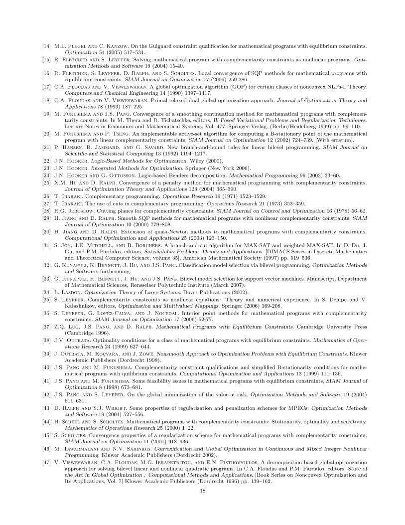
Figures 1, 2 and 3 detail the progress of the runs, showing in particular how LPCCub decreases with the numberof iterations. The vertical axis refers to the LPCC objective values and the horizontal axis labels the number ofiterations as defined in the opening paragraph of Section 5. The top value on the vertical axis is the LPCC objectivevalue obtained at termination of the pre-processor with the LPCC feasibility recovery step. The bottom value isverifiably LPECmin. The vertical axis is scaled differently in each run with respect to the difference between thetop and the bottom values. As comparison, the objective values obtained from filter (marked by the red square)and knitro (marked by the blue diamond) are also shown on the vertical axis; if the difference between the filterand knitro values in a run is within 1e-3, we only mark the knitro result (the exact values from these two solverscan be found in Tables 1, 2 and 3). The upper limit of the horizontal axis indicates the number of IPs needed tobe solved in each run. Note that in some runs, a globally optimal solution might have been obtained in an earlieriteration without certification, and the algorithm needs more subsequent iterations to verify its global optimality.For example, in the fourth run of the right-hand column in Figure 1, a globally optimal solution is first obtainedat iteration 2, but the certificate is established only after 23 more iterations. Other details about the figures aresummarized in the remarks below the figures.

Corresponding to the problems in Figures 1, 2 and 3 respectively, Tables 1, 2 and 3 report more details aboutthe runs, which are indexed by counting first row-wise and then column-wise in the figures (for example, the fourthrun in Table 1 is the second row on the right column in Figure 1). In addition to the objective values obtained inour algorithm and from the neos solvers, these tables also report the numbers of IPs and LPs (excluding the bm/3crelaxed LPs solved in the pre-processor), solved in the solution process. These numbers, which are independentof the computational platform and machine, provide a good indicator of the efforts required by the algorithm inprocessing the LPCCs. We did not report computational times for two reasons: (i) the matlab results are computerdependent and the runs involve interfaces between matlab and cplex, and (ii) our runs are experimental and ourcoding is at an amateur level.

The computational results for the infeasible and unbounded LPCCs are reported in Table 4, which contains 3sub-tables (a), (b), and (c). The first two sub-tables (a) and (b) pertain to feasible but unbounded LPCCs. Forthe unbounded problems, we set B = 0, q is arbitrary, and we generate A with a nonnegative column, M givenby (6.1) and f such that {x ≥ 0 : Ax ≥ f} is feasible. Problems in (a) and (b) have the same parameters exceptfor the objective vector c and d and matrix A. For the problems in (a), we simply maximize one single x-variablewhose A column is nonnegative. For the problems in (b), the objective vectors c and d are both negative; and thematrix A is the same as it is in group (a) except that a small number 0.005 is added to its nonnegative column(see the discussion in the first conclusion below for why this is done). The third sub-table (c) pertains to a classof infeasible LPCCs generated as follows: q, N , and M are all positive so that the only solution to the LCP:0 ≤ y ⊥ q +Nx+My ≥ 0 for x ≥ 0 is y = 0; Ax+ By ≥ f is feasible for some (x, y) ≥ 0 with y 6= 0 but Ax ≥ fhas no solution in x ≥ 0.

To illustrate the effectiveness of the sparsification step, we generated some LPCCs with n = m = k = 25 andthe same characteristics as the problems in Figure 3. Table 5 reports the numbers of LPs and IPs that are neededto be solved in both runs with or without this step.

The main conclusions from the experiments are summarized below.

• The algorithm successfully terminates with the correct status of all the LPCCs reported. In fact, we have testedmany more problems than those reported and obtained similar success. There are, nevertheless, a few instanceswhere the LPCC are apparently unbounded but the algorithm fails to terminate after 6,000 iterations withoutthe definitive conclusion, even though the LPCC objective is noticeably tending to −∞. We cannot explain theseexceptional cases which we suspect are due to round-off errors in the computations. This suspicion led us to addthe small 0.005 in the unbounded set of runs reported above; with this small adjustment, the algorithm successfullyterminated with the desired certificate of unboundedness.

• For the special LPCCs with B = 0, the results from the two neos algorithms, filter and knitro, are provedto be suboptimal in 2 out of the 20 runs (the first and fourth runs on the left column in Figure 1). In the other 18

16

runs, our algorithm is able to obtain an optimal solution with little computational effort (within 5 iterations), butrequires significant additional computations to produce the desired certificate of global optimality. For the generalLPCCs with B 6= 0, the objective values obtained from filter and knitro are suboptimal in 6 out of 10 runs.In the other 4 runs, only 5 iterations are needed to derive either a globally optimal solution or an LPCC feasiblesolution whose objective value is within 3% of the optimal value. These results confirm that the verification of globaloptimality is generally much more demanding than the computation of the solution without proof of optimality.

• Except for one problem (problem 7 in Table 3), the solutions obtained by the simple-cut pre-processor for allLPCCs with finite optima are within 5% of the globally optimal solutions. In fact, some of the solutions obtainedfrom the pre-processing are immediately verified to be optimal. This suggests that very high-quality LPCC feasiblesolutions can be produced efficiently by solving a reasonable number of LPs.

• The sparsification procedure is quite effective; so is the LPCC feasibility recovery step. Indeed without the latter,there is a significant percentage of problems where the algorithm fails to make progress after 3,000 iterations. Withthis step installed, all problems are resolved satisfactorily.

• While the numbers of IPs solved are quite reasonable in most cases, there are several runs where the numbersof relaxed LPs solved are unusually large, especially when the problem size increases. This suggests that strongercuts are needed for both general LPCCs and for specialized problems arising from large-scale applications. Theimplementation of a dedicated solver for satisfiability problems, such as those described in [7, 31], could considerablyimprove the overall solution times of the LPCC algorithm. These refinements of the algorithm are presently beinginvestigated.

Concluding remarks. In this paper, we have presented a parameter-free IP based algorithm for the globalresolution of an LPCC and reported computational results with the application of the algorithm for solving a setof randomly generated LPCCs of moderate sizes. Continued research on refining the algorithm and applying it torealistic classes of LPCCs, such as the bilevel machine learning problems described in [6, 32, 33] and other appliedproblems, is currently underway.

Acknowledgements. The authors are grateful to 2 referees for their constructive comments that have significantlyimprove the presentation of the paper. In particular, one of them alerted the authors to the reference [9] thatdiscusses Benders techniques for conditional linear constraints without requiring the big-M.

REFERENCES

[1] M. Anitescu. On using the elastic mode in nonlinear programming approaches to mathematical programs with complementarityconstraints. SIAM Journal on Optimization 15 (2005) 1203–1236.

[2] M. Anitescu. Global convergence of an elastic mode approach for a class of mathematical programs with complementarityconstraints. SIAM Journal on Optimization 16 (2005) 120–145.

[3] M. Anitescu, P. Tseng, and S.J. Wright. Elastic-mode algorithms for mathematical programs with equilibrium constraints:Global convergence and stationarity properties. Mathematical Programming 110 (2007) 337–371.

[4] C. Audet, P. Hansen, B. Jammard, and G. Savard. Links between linear bilevel and mixed 0–1 programming problems.Journal of Optimization Theory and Applications 93 (1997) 273–300.

[5] C. Audet, G. Savard, and W. Zghal. New branch-and-cut algorithm for bilevel linear programming, Journal of OptimizationTheory and Applications 134 (2007) 353–370.

[6] K. Bennett, X. Ji, J. Hu, G. Kunapuli, and J.S. Pang. Model selection via bilevel programming, Proceedings of the Interna-tional Joint Conference on Neural Networks (IJCNN’06) Vancouver, B.C. Canada, July 16–21, 2006 pp.

[7] B. Borchers and J. Furman. A two-phase exact algorithm for MAX-SAT and weighted MAX-SAT Problems. Journal ofCombinatorial Optimization 2 (1998) 299–306.

[8] L. Chen and D. Goldfarb. An active-set method for mathematical programs with linear complementarity constraints.Manuscript, Department of Industrial Engineering and Operations Research, Columbia University (January 2007).

[9] G. Codato and M. Fischetti. Combinatorial Benders’ Cuts for mixed-integer linear programming. Operations Research 54(2006) 758–766.

[10] R.W. Cottle, J.S. Pang, and R.E. Stone. The Linear Complementarity Problem, Academic Press, Boston (1992)

[11] S. Dempe. Foundations of bilevel programming. Kluwer Academic Publishers (Dordrecht, The Netherlands 2002).

[12] S. Dempe. Annotated bibliography on bilevel programming and mathematical programs with equilibrium constraints. Optimiza-tion 52 (2003) 333–359.

[13] S. Dempe, V.V. Kalashnikov, and N. Kalashnykova. Optimality conditions for bilevel programming problems. In S. Dempeand N. Kalashnykova, editors, Optimization with Multivalued Mappings: Theory, Applications and Algorithms. Springer-Verlag New York Inc. (New York 2006) pp. 11–36.

17

[14] M.L. Flegel and C. Kanzow. On the Guignard constraint qualification for mathematical programs with equilibrium constraints.Optimization 54 (2005) 517–534.

[15] R. Fletcher and S. Leyffer. Solving mathematical program with complementarity constraints as nonlinear programs. Opti-mization Methods and Software 19 (2004) 15-40.

[16] R. Fletcher, S. Leyffer, D. Ralph, and S. Scholtes. Local convergence of SQP methods for mathematical programs withequilibrium constraints. SIAM Journal on Optimization 17 (2006) 259-286.

[17] C.A. Floudas and V. Visweswaran. A global optimization algorithm (GOP) for certain classes of nonconvex NLPs-I. Theory.Computers and Chemical Engineering 14 (1990) 1397–1417.

[18] C.A. Floudas and V. Visweswaran. Primal-relaxed dual global optimization approach. Journal of Optimization Theory andApplications 78 (1993) 187–225.

[19] M. Fukushima and J.S. Pang. Convergence of a smoothing continuation method for mathematical programs with complemen-tarity constraints. In M. Thera and R. Tichatschke, editors, Ill-Posed Variational Problems and Regularization Techniques.Lecture Notes in Economics and Mathematical Systems, Vol. 477, Springer-Verlag, (Berlin/Heidelberg 1999) pp. 99–110.

[20] M. Fukushima and P. Tseng. An implementable active-set algorithm for computing a B-stationary point of the mathematicalprogram with linear complementarity constraints. SIAM Journal on Optimization 12 (2002) 724–739. [With erratum].

[21] P. Hansen, B. Jammard, and G. Savard. New branch-and-bound rules for linear bilevel programming. SIAM Journal onScientific and Statistical Computing 13 (1992) 1194–1217.

[22] J.N. Hooker. Logic-Based Methods for Optimization. Wiley (2000).

[23] J.N. Hooker. Integrated Methods for Optimization. Springer (New York 2006).

[24] J.N. Hooker and G. Ottosson. Logic-based Benders decomposition. Mathematical Programming 96 (2003) 33–60.

[25] X.M. Hu and D. Ralph. Convergence of a penalty method for mathematical programming with complementarity constraints.Journal of Optimization Theory and Applications 123 (2004) 365–390.

[26] T. Ibaraki. Complementary programming. Operations Research 19 (1971) 1523–1529.

[27] T. Ibaraki. The use of cuts in complementary programming. Operations Research 21 (1973) 353–359.

[28] R.G. Jeroslow. Cutting planes for complementarity constraints. SIAM Journal on Control and Optimization 16 (1978) 56–62.

[29] H. Jiang and D. Ralph. Smooth SQP methods for mathematical programs with nonlinear complementarity constraints. SIAMJournal of Optimization 10 (2000) 779–808.

[30] H. Jiang and D. Ralph. Extension of quasi-Newton methods to mathematical programs with complementarity constraints.Computational Optimization and Applications 25 (2003) 123–150.

[31] S. Joy, J.E. Mitchell, and B. Borchers. A branch-and-cut algorithm for MAX-SAT and weighted MAX-SAT. In D. Du, J.Gu, and P.M. Pardalos, editors, Satisfiability Problem: Theory and Applications. [DIMACS Series in Discrete Mathematicsand Theoretical Computer Science, volume 35], American Mathematical Society (1997) pp. 519–536.

[32] G. Kunapuli, K. Bennett, J. Hu, and J.S. Pang. Classification model selection via bilevel programming, Optimization Methodsand Software, forthcoming.

[33] G. Kunapuli, K. Bennett, J. Hu, and J.S. Pang. Bilevel model selection for support vector machines. Manuscript, Departmentof Mathematical Sciences, Rensselaer Polytechnic Institute (March 2007).

[34] L. Lasdon. Optimization Theory of Large Systems. Dover Publications (2002).

[35] S. Leyffer. Complementarity constraints as nonlinear equations: Theory and numerical experience. In S. Dempe and V.Kalashnikov, editors, Optimization and Multivalued Mappings. Springer (2006) 169-208.

[36] S. Leyffer, G. Lopez-Calva, and J. Nocedal. Interior point methods for mathematical programs with complementarityconstraints. SIAM Journal on Optimization 17 (2006) 52-77.

[37] Z.Q. Luo, J.S. Pang, and D. Ralph. Mathematical Programs with Equilibrium Constraints. Cambridge University Press(Cambridge 1996).

[38] J.V. Outrata. Optimality conditions for a class of mathematical programs with equilibrium constraints. Mathematics of Oper-ations Research 24 (1999) 627–644.

[39] J. Outrata, M. Kocvara, and J. Zowe. Nonsmooth Approach to Optimization Problems with Equilibrium Constraints. KluwerAcademic Publishers (Dordrecht 1998).

[40] J.S. Pang and M. Fukushima. Complementarity constraint qualifications and simplified B-stationarity conditions for mathe-matical programs with quilibrium constraints, Computational Optimization and Applications 13 (1999) 111–136.

[41] J.S. Pang and M. Fukushima. Some feasibility issues in mathematical programs with equilibrium constraints, SIAM Journal ofOptimization 8 (1998) 673–681.

[42] J.S. Pang and S. Leyffer. On the global minimization of the value-at-risk, Optimization Methods and Software 19 (2004)611–631.

[43] D. Ralph and S.J. Wright. Some properties of regularization and penalization schemes for MPECs. Optimization Methodsand Software 19 (2004) 527–556.

[44] H. Scheel and S. Scholtes. Mathematical programs with complementarity constraints: Stationarity, optimality and sensitivity.Mathematics of Operations Research 25 (2000) 1–22.

[45] S. Scholtes. Convergence properties of a regularization scheme for mathematical programs with complementarity constraints.SIAM Journal on Optimization 11 (2001) 918–936.

[46] M. Tawarmalani and N.V. Sahinidis. Convexification and Global Optimization in Continuous and Mixed Integer NonlinearProgramming. Kluwer Academic Publishers (Dordrecht 2002).

[47] V. Visweswaran, C.A. Floudas, M.G. Ierapetritou, and E.N. Pistikopoulos. A decomposition based global optimizationapproach for solving bilevel linear and nonlinear quadratic programs. In C.A. Floudas and P.M. Pardalos, editors. State ofthe Art in Global Optimization : Computational Methods and Applications. [Book Series on Nonconvex Optimization andIts Applications, Vol. 7] Kluwer Academic Publishers (Dordrecht 1996) pp. 139–162.

18

[48] J.J. Ye. Optimality conditions for optimization problems with complementarity constraints. SIAM Journal on Optimization 9(1999) 374–387.

[49] J.J. Ye. Constraint qualifications and necessary optimality conditions for optimization problems with variational inequalityconstraints. SIAM Journal on Optimization 10 (2000) 943–962.

[50] J.J. Ye. Necessary and sufficient optimality conditions for mathematical programs with equilibrium constraints. Journal ofMathematical Analysis and Applications 30 (2005) 350–369.

19

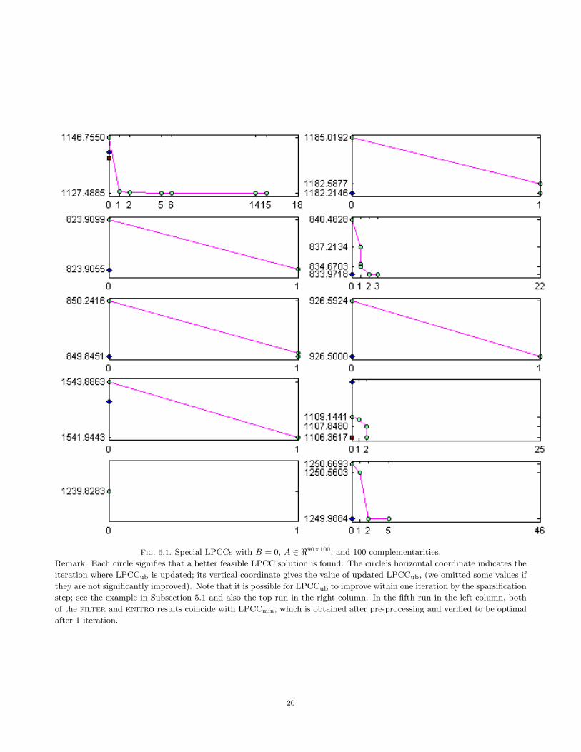
Fig. 6.1. Special LPCCs with B = 0, A ∈ <90×100, and 100 complementarities.

Remark: Each circle signifies that a better feasible LPCC solution is found. The circle’s horizontal coordinate indicates the

iteration where LPCCub is updated; its vertical coordinate gives the value of updated LPCCub, (we omitted some values if

they are not significantly improved). Note that it is possible for LPCCub to improve within one iteration by the sparsification

step; see the example in Subsection 5.1 and also the top run in the right column. In the fifth run in the left column, both

of the filter and knitro results coincide with LPCCmin, which is obtained after pre-processing and verified to be optimal

after 1 iteration.

20

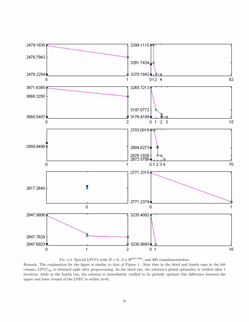
Fig. 6.2. Special LPCCs with B = 0, A ∈ <200×300, and 300 complementarities.

Remark: The explanation for the figure is similar to that of Figure 1. Note that in the third and fourth runs in the left

column, LPCCub is obtained right after preprocessing. In the third run, the solution’s global optimality is verified after 1

iteration; while in the fourth run, the solution is immediately verified to be globally optimal (the difference between the

upper and lower bound of the LPEC is within 1e-6).

21

Fig. 6.3. General LPECs with B 6= 0, A ∈ <55×50, and 50 complementarities.

22

LPCClb LPCCub

Prob relaxed LP preprocess preprocess LPCCmin filter knitro LPs IPs

1 1094.6041+12.2255 1106.8297 1146.7550−19.2665 1127.4885 1140.5614 5 1141.6696 52 396 18

2 1172.1830+4.5063 1176.6893 1185.0192−2.8046 1182.2146 1182.2145 5 1182.2147 47 57 1

3 820.2584+3.6328 823.8912 823.9099−0.0044 823.9055 823.9055 10 823.9058 55 14 1

4 796.9560+17.0192 813.9752 840.4828−6.5110 833.9718 833.9717 6 833.9718 41 611 22

5 841.1786+7.8336 849.0122 850.2416−0.3965 849.8451 849.8451 5 849.8452 44 66 1

6 924.7529+1.3500 926.1028 926.5924−0.0923 926.5000 926.5000 5 926.5000 56 21 1

7 1536.1748+5.2715 1541.4464 1543.8863−1.9419 1541.9443 1543.1950 6 1543.1951 55 35 1

8 1076.8760+13.3395 1090.2155 1109.1441−2.7824 1106.3617 1106.3616 5 1113.8938 70 363 25

9 1232.7912+6.9243 1239.7156 1239.8283 1239.8283 1239.8284 7 1239.8285 62 10 1

10 1217.1191+12.1543 1229.2734 1250.6693−0.6808 1249.9884 1249.9884 8 1249.9886 67 832 46Table 6.1

Special LPECs with B = 0, A ∈ <90×100, and 100 complementarities.

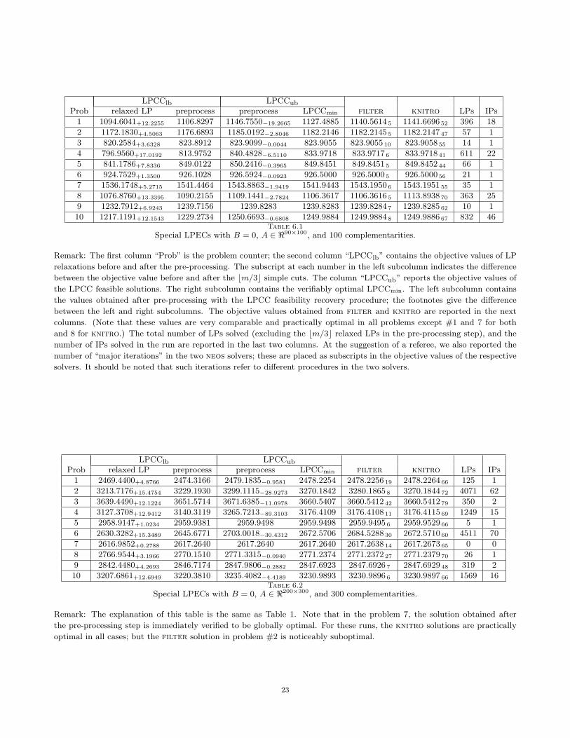
Remark: The first column “Prob” is the problem counter; the second column “LPCClb” contains the objective values of LP

relaxations before and after the pre-processing. The subscript at each number in the left subcolumn indicates the difference

between the objective value before and after the bm/3c simple cuts. The column “LPCCub” reports the objective values of

the LPCC feasible solutions. The right subcolumn contains the verifiably optimal LPCCmin. The left subcolumn contains

the values obtained after pre-processing with the LPCC feasibility recovery procedure; the footnotes give the difference

between the left and right subcolumns. The objective values obtained from filter and knitro are reported in the next

columns. (Note that these values are very comparable and practically optimal in all problems except #1 and 7 for both

and 8 for knitro.) The total number of LPs solved (excluding the bm/3c relaxed LPs in the pre-processing step), and the

number of IPs solved in the run are reported in the last two columns. At the suggestion of a referee, we also reported the

number of “major iterations” in the two neos solvers; these are placed as subscripts in the objective values of the respective

solvers. It should be noted that such iterations refer to different procedures in the two solvers.

LPCClb LPCCub

Prob relaxed LP preprocess preprocess LPCCmin filter knitro LPs IPs

1 2469.4400+4.8766 2474.3166 2479.1835−0.9581 2478.2254 2478.2256 19 2478.2264 66 125 1

2 3213.7176+15.4754 3229.1930 3299.1115−28.9273 3270.1842 3280.1865 8 3270.1844 72 4071 62

3 3639.4490+12.1224 3651.5714 3671.6385−11.0978 3660.5407 3660.5412 42 3660.5412 79 350 2

4 3127.3708+12.9412 3140.3119 3265.7213−89.3103 3176.4109 3176.4108 11 3176.4115 69 1249 15

5 2958.9147+1.0234 2959.9381 2959.9498 2959.9498 2959.9495 6 2959.9529 66 5 1

6 2630.3282+15.3489 2645.6771 2703.0018−30.4312 2672.5706 2684.5288 30 2672.5710 60 4511 70

7 2616.9852+0.2788 2617.2640 2617.2640 2617.2640 2617.2638 14 2617.2673 65 0 0

8 2766.9544+3.1966 2770.1510 2771.3315−0.0940 2771.2374 2771.2372 27 2771.2379 70 26 1

9 2842.4480+4.2693 2846.7174 2847.9806−0.2882 2847.6923 2847.6926 7 2847.6929 48 319 2

10 3207.6861+12.6949 3220.3810 3235.4082−4.4189 3230.9893 3230.9896 6 3230.9897 66 1569 16Table 6.2

Special LPECs with B = 0, A ∈ <200×300, and 300 complementarities.

Remark: The explanation of this table is the same as Table 1. Note that in the problem 7, the solution obtained after

the pre-processing step is immediately verified to be globally optimal. For these runs, the knitro solutions are practically

optimal in all cases; but the filter solution in problem #2 is noticeably suboptimal.

23

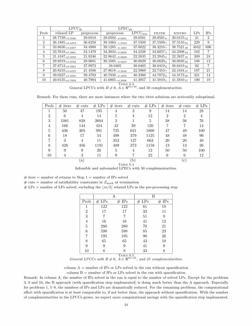
LPCClb LPECub

Prob relaxed LP preprocess preprocess LPCCmin filter knitro LPs IPs

1 28.7739+0.2580 29.0318 29.0502−0.0001 29.0501 29.0501 8 30.0155 32 21 2

2 36.1885+0.6373 36.8258 39.1063−1.5554 37.5509 37.5509 7 37.5510 25 229 9

3 33.8630+0.6357 34.4988 39.1285−2.1263 37.0022 38.3216 7 38.7521 28 4842 696

4 33.7618+0.3861 34.1479 34.3034−0.0806 34.2228 34.6057 5 34.2398 54 102 7

5 21.4187+0.5059 21.9246 22.9642−0.6806 22.2835 22.2945 5 22.2837 35 209 24

6 29.8919+0.0762 29.9681 30.1085−0.0255 30.0829 30.0829 6 30.0830 26 108 13

7 37.6712+0.3261 37.9972 38.0405 38.0405 38.0419 6 38.0419 29 92 7

8 20.8210+0.6375 21.4586 27.9618−5.5649 22.3969 22.7453 7 22.4164 37 187 21

9 39.0227+0.4565 39.4792 40.7839−0.4459 40.3380 44.7872 8 44.3173 26 321 14

10 40.0135+0.7859 40.7994 41.6865−0.2908 41.3957 41.5810 5 41.5810 37 190 19Table 6.3

General LPCCs with B 6= 0, A ∈ <55×50, and 50 complementarities.

Remark: For these runs, there are more instances where the two neos solutions are noticeably suboptimal.

Prob # iters # cuts # LPs # iters # cuts # LPs # iters # cuts # LPs1 50 47 195 4 3 9 14 14 282 6 4 14 5 4 12 2 2 43 1081 828 2604 2 1 5 38 38 764 166 144 424 42 39 120 7 7 145 436 305 991 735 621 1860 47 49 1006 18 17 54 498 379 1125 48 48 967 3 4 11 352 127 663 20 20 408 426 356 1191 489 373 1158 13 13 269 9 9 26 5 4 12 50 50 10010 4 3 11 9 7 22 6 6 12

(a) (b) (c)Table 6.4

Infeasible and unbounded LPECs with 50 complementarities.

# iters = number of returns to Step 1 = number of IPs solved

# cuts = number of satisfiability constraints in Zwork at termination

# LPs = number of LPs solved, excluding the bm/3c relaxed LPs in the pre-processing step

A BProb # LPs # IPs # LPs # IPs

1 122 122 61 182 17 17 33 113 7 7 51 94 16 16 41 125 280 280 70 216 598 598 85 237 195 195 90 268 65 65 43 109 9 9 41 910 8 8 33 8

Table 6.5General LPCCs with B 6= 0, A ∈ <25×25, and 25 complementarities.

column A = number of IPs or LPs solved in the run without sparsification

column B = number of IPs or LPs solved in the run with sparsification

Remark: In column A, the number of IPs solved in the run is equal to the number of solved LPs. Except for the problems

3, 9 and 10, the B approach (with sparsification step implemented) is doing much better than the A approach. Especially

for problems 1, 5–8, the numbers of IPs and LPs are dramatically reduced. For the remaining problems, the computational

effort with sparsification is at least comparable to, if not better than, the approach without sparsification. With the number

of complementarities in the LPCCs grows, we expect more computational savings with the sparsification step implemented.

24