Smooth methods of multipliers for complementarity problems

Digital Object Identifier (DOI) 10.1007/s101079900076

Math. Program., Ser. A 86: 65–90 (1999) Springer-Verlag 1999

Jonathan Eckstein·Michael C. Ferris

Smooth methods of multipliers for complementarityproblems

Received February 21, 1997 / Revised version received December 11, 1998Published online May 12, 1999

Abstract. This paper describes several methods for solving nonlinear complementarity problems. A generalduality framework for pairs of monotone operators is developed and then applied to the monotone comple-mentarity problem, obtaining primal, dual, and primal-dual formulations. We derive Bregman-function-basedgeneralized proximal algorithms for each of these formulations, generating three classes of complementarityalgorithms. The primal class is well-known. The dual class is new and constitutes a general collection ofmethods of multipliers, or augmented Lagrangian methods, for complementarity problems. In a special case,it corresponds to a class of variational inequality algorithms proposed by Gabay. By appropriate choice ofBregman function, the augmented Lagrangian subproblem in these methods can be made continuously dif-ferentiable. The primal-dual class of methods is entirely new and combines the best theoretical features ofthe primal and dual methods. Some preliminary computation shows that this class of algorithms is effectiveat solving many of the standard complementarity test problems.

Key words. complementarity problems – smoothing – proximal algorithms – augmented Lagrangians

1. Introduction

This paper concerns the solution of thenonlinear complementarity problem(NCP). Letl ∈ [−∞,∞)n andu ∈ (−∞,∞]n, with l ≤ u. Suppose{x ∈ <n | l ≤ x ≤ u} ⊆D ⊆ <n, and letF : D → <n be continuous. Then, the NCP is to find somex ∈ <n

satisfying the conditions

l ≤ x ≤ u mid(l, x− F(x),u) = x, (1)

where mid(a,b, c) denotes the componentwise median of the vectorsa, b, andc. Thisproblem is a special case of the standardvariational inequalityproblem: givenF anda setC ⊆ <n, find somex such that

x ∈ C⟨F(x), y− x

⟩ ≥ 0 ∀ y ∈ C . (2)

If we takeC = {x ∈ <n | l ≤ x ≤ u}, then (2) is identical to (1).The special case ofl = 0 andu = ∞ reduces (1) to

x ≥ 0 max(x− F(x),0) = x,

J. Eckstein: Faculty of Management and RUTCOR, Rutgers University, 640 Bartholomew Road, Piscataway,NJ 08854, e-mail:[email protected] .The research was partially supported by a Rutgers University Faculty of Management Research ResourcesFellowship.

M.C. Ferris: University of Wisconsin, Computer Sciences Department, 1210 West Dayton Street, Madison,WI 53706, e-mail:[email protected] .The research was partially supported by National Science Foundation Grant CCR-9619765.

66 Jonathan Eckstein, Michael C. Ferris

or equivalently

x ≥ 0 F(x) ≥ 0⟨x, F(x)

⟩ = 0. (3)

If the mappingF is affine, then (3) is the classicallinear complementarity problem, orLCP.

In the theoretical portion of this paper, we will restrict our attention to themonotonecase in whichF satisfies⟨

F(x)− F(y), x− y⟩ ≥ 0 ∀ x, y ∈ <n. (4)

This assumption will allow us to model (1) as the problem of finding a root of the sumof two monotone operators (seee.g.[3]), as will be explained in Section 2. To find sucha root, we then apply generalized proximal algorithms based on Bregman functions [6,7,9,12,17,18,33].

A number of recent papers [5,6,8] have stressed the ability of proximal terms arisingfrom appropriately-formulated Bregman functions to act like barrier functions, givingrise to “interior point” proximal methods for variational inequality problems. Suchmethods are derived by applying Bregman proximal methods to a primal formulationof (1) or (2).

In contrast, we emphasize dual and primal-dual formulations. Applying Bregmanproximal methods to such formulations yields augmented-Lagrangian-like algorithms,or “methods of multipliers.” In the dual case, we obtain a class of methods generaliz-ing [21, “ALG1”]. By careful choice of Bregman function, we generate methods whichinvolve solving (provided thatF is differentiable) a once-differentiable system of equa-tions at each iteration, as opposed to a nonsmooth system, as in [21]. Therefore, we canuse a standard algorithm such as Newton’s method to solve these subproblems. A similarphenomenon has already been pointed out for smooth convex programming problemsin [24]. That paper notes that one of the augmented Lagrangian methods proposedin [17] yields a twice-differentiable augmented Lagrangian, as opposed to the classicalonce-differentiable augmented Lagrangian for inequality constraints (e.g.[30]).

In producing sequences of subproblems consisting of differentiable nonlinear equa-tions, our algorithms bear some resemblance to recently proposed smoothing methodsfor the LCP and NCP [10,11,22]. However, such methods are akin to pure penaltymethods in constrained optimization — they have a penalty parameter that must bedriven to infinity to obtain convergence. By contrast, our algorithms are generalizedversions of augmented Lagrangian methods: there is a Lagrange multiplier adjustmentat the end of each iteration, and we obtain convergence even if the penalty parameterdoes not approach infinity.

In the course of our derivation, Section 2 develops a simple duality frameworkfor pairs of set-valued operators. The framework resembles [1], but allows the twomappings in the pair to operate on different spaces. A similar duality structure for pairsof monotone operators appears in [20]. The main distinction of our approach, as opposedto [1,20], is to introduce a primal-dual, “saddle-point” formulation, in addition to thestandard primal and dual formulations. Towards the end of Section 2, we show how toapply the duality framework to variational inequalities and complementarity problems,refining the framework for variational inequalities that appears in [21,27].

Smooth methods of multipliers for complementarity problems 67

Section 3 combines the duality framework of Section 2 with Bregman functionproximal algorithms and shows how to produce new, smooth methods of multipliersfor (1). The primal-dual formulation yields a newproximalmethod of multipliers for (1),along the lines of the proximal method of multipliers for convex programming (e.g.[30]).This primal-dual method combines the best theoretical features of primal methods inthe spirit of [5,6,8] with the best features of the new dual method. Some preliminarycomputational results on the MCPLIB [14] suite of test problems are given in Section 4.These results show that proximal method of multipliers is effective even when theunderlying problem is not monotone.

2. A simple duality framework for pairs of monotone operators

In this paper, anoperatorT on a real Hilbert spaceX is a subset ofX × Y, whereY isalso a Hilbert space. We callY therange spaceof T; typically, but not always, we willhaveX = Y.

For every suchT ⊆ X×Y andx ∈ X, T(x).= {y ∈ Y | (x, y) ∈ T } defines a point-

to-set mapping fromX to Y; in fact, we make no distinction between this point-to-setmapping and its graphT. Thus, the statementsy ∈ T(x) and(x, y) ∈ T are completelyequivalent. Theinverseof any operatorT is T−1 = {(y, x) ∈ Y× X | (x, y) ∈ T },which will always exist. Trivially,(T−1)−1 = T. We define

domT.= {x | T(x) 6= ∅} = {x ∈ X | ∃ y ∈ Y : (x, y) ∈ T } ,

and similarly imT.= dom(T−1) = {y ∈ Y | ∃ x ∈ X : (x, y) ∈ T }. When T(x) is

a singleton set{y} for all x, that is,T is the graph of some function domT → Y,we say thatT is single-valued, and we may write, in a slight abuse of notation,T(x) = yinstead ofT(x) = {y}.

Given two operatorsT andU on X with the same range spaceY, their sumT +Uis defined via(T + U)(x) = T(x)+ U(x) = {t + u | t ∈ T(x),u ∈ U(x)}. If T is anyoperator onX andU an operator onZ, we define theirdirect productT ⊗U on X× Zvia (T ⊗U)(x, z) = T(x)×U(z).

An operatorT on X is said to bemonotoneif its range space isX and⟨x− x′, y− y′

⟩ ≥ 0 ∀ (x, y), (x′, y′) ∈ T. (5)

Note that (5) is a natural generalization of (4): if one takesX = <n andT to be thegraph of the functionF, (5) reduces to (4). Note also that monotonicity ofT andT−1

are equivalent, and that it is straightforward to show that if two operatorsT andU areboth monotone, then so isT +U.

A monotone operatorT is maximalif no strict superset ofT is monotone, that is,

(x, y) ∈ X × X,⟨x− x′, y− y′

⟩ ≥ 0 ∀ (x′, y′) ∈ T ⇒ (x, y) ∈ T.

Maximality of an operator and maximality of its inverse are equivalent.The fundamental problem customarily associated with a monotone operatorT is

that of finding azeroor root, that is, somex ∈ X such that 0∈ T(x) (seee.g.[3,31]).


2.1. The duality framework

Suppose we are given an operatorA on a Hilbert spaceX, an operatorB on a HilbertspaceY, and a linear mappingM : X→ Y. We will denote such a triple byP(A, B,M).For the development in Section 3, we will require only the special caseX = Y = <n andM = I , but we consider the generalP(A, B,M) in order to make connections to [16,20] and other previous work.

We associate withP(A, B,M) a primal formulationof finding x ∈ X such that

0 ∈ A(x)+ M>B(Mx), (6)

or equivalently 0∈ TP(x).= [A+ M>BM

](x), whereM> denotes the adjoint ofM.

Similarly, we associate with eachP(A, B,M) a dual formulationof finding y ∈ Ysuch that

0 ∈ −MA−1(−M>y)+ B−1(y), (7)

or equivalently 0∈ TD(y).= [−MA−1(−M>)+ B−1

](y). Note that (7) is the primal

formulation ofP(B−1, A−1,−M>), and that twice applying the transformation

P(A, B,M) 7→ P(B−1, A−1,−M>)

produces the original tripleP(A, B,M); that is, the dual ofP(B−1, A−1,−M>) is theoriginal primal formulation (6). The duality scheme of [1] is similar, with the restrictionsX = Y andM = I .

We also associate withP(A, B,M) a primal-dual formulation, which is to find(x, y) ∈ X× Y such that

0 ∈ A(x)+ M>y 0 ∈ −Mx+ B−1(y), (8)

or equivalently 0∈ TPD(x, y).= K [A, B,M](x, y), whereK [A, B,M] is defined by

K [A, B,M](

xy

)=(

A(x)× B−1(y))+[

0 M>

−M 0

](xy

). (9)

In the special case of convex optimization, we can takeA = ∂ f , the subdifferentialmap of some closed proper convex functionf : X→ (−∞,+∞], andB = ∂g for someclosed proper convexg : Y→ (−∞,+∞]. Then the primal formulation is equivalentto the optimization problem

minx∈X

f(x)+ g(Mx). (10)

Similarly, the dual formulation is equivalent to

miny∈Y

f ∗(−M>y)+ g∗(y), (11)

where “∗” denotes the convex conjugacy operation [28, Section 12]. Furthermore, thesubdifferential of the generalized LagrangianL : X × Y→ [−∞,+∞] defined by

L(x, y) = f(x)+ 〈y,Mx〉 − g∗(y)


is preciselyK [A, B,M] = K [∂ f , ∂g,M]. Therefore, the primal-dual formulation isequivalent to finding a saddle point ofL, that is, to the problem

minx∈X

maxy∈Y

f(x)+ y>Mx − g∗(y). (12)

The standard convex programming duality relations between (10), (11), and (12) maybe viewed as a consequence of the higher-level, more abstract duality embodied in thefollowing elementary proposition, whose proof is omitted.

Proposition 1. The following statements are equivalent:

(i) (x, y) solves the primal-dual formulation (8).(ii) x ∈ X, y ∈ Y, (x,−M>y) ∈ A, (Mx, y) ∈ B.

Furthermore,x solves the primal formulation (6) if and only if there existsy ∈ Y suchthat (i)-(ii) hold, andy solves the dual formulation (7) if and only if there existsx ∈ Xsuch that (i)-(ii) hold.

Note that for general choices ofA, B, and M, this duality framework is slightlyweaker than, for example, linear programming, in thatx being a primal solution andybeing a dual solution arenot sufficient for(x, y) to be an solution of the primal-dual(“saddle point”) formulation, even ifA andB are maximal monotone. For an exampleof this phenomenon, consider the caseX = Y = <2, M = I , A(x1, x2) = {(−x2, x1)},andB(x1, x2) = {(x2,−x1)}.

We now turn to the issue of solving (6), (7) or (8), under the assumption thatA andBare maximal monotone.

Consider first the primal formulation (6). Given thatB is monotone, it is straight-forward to show thatM>BM is also monotone. The monotonicity ofA then gives themonotonicity ofTP = A+ M>BM. Therefore, the primal formulation is a problem oflocating a root of the monotone operatorTP on X. The convergence analyses of root-finding methods for monotone operators typically require that the operator be not onlymonotone, but also maximal. WhileTP will typically be maximal if A andB are, suchmaximality cannot be guaranteed without imposing additional regularity conditions.Some typical sufficient conditions forTPto be maximal are thatAandBbe maximal, thatMM> be an isomorphism ofY, thus guaranteeing maximality ofM>BM (see [21, Propo-sition 4.1] or [20, Proposition 3.2]), and a condition such as domA ∩ int dom(BM) 6= ∅,in order to ensure maximality of the sumTP = A+ M>BM [29]. This last conditioncan be weakened somewhat ifX is finite-dimensional.

The analysis of the dual formulation is similar. The formulation involves locating theroot of the operatorTD = −MA−1(−M>)+B−1 onY, which is necessarily monotone bythe monotonicity ofA andB, but is not guaranteed to be maximal solely by maximalityof A andB. One must impose similar conditions to the primal case, such asM>M beingan isomorphism ofX, and dom(A−1(−M>)) ∩ int im B 6= ∅.

The primal-dual formulation also involves finding the root of a monotone operator:we establish in Proposition 2 below that the operatorTPD = K [A, B,M] on X × Y(with the canonical inner product induced byX andY) is monotone ifA and B are.The proposition also shows that the primal-dual is in some sense the “best behaved” ofour three formulations, in the sense thatK [A, B,M] is maximal wheneverA andB areboth maximal.


Proposition 2. If A and B are monotone operators on the Hilbert spacesX and Y,respectively, andM is any linear mapX→ Y, then the operatorK [A, B,M] on X×Ydefined by (9) is monotone. Furthermore, ifA and B are both maximal,K [A, B,M] ismaximal.

Proof. Set

T1 = A⊗ B−1 T2(x, y) =[

0 M>

−M 0

](xy

).

Note thatT1 andT2 are both monotone, andK [A, B,M] = T1 + T2. If A and B aremaximal,T1 is also maximal. The linear mapT2 is also maximal [26], and maximalityof T1+ T2 then follows from [29, Theorem 1(a)].

We remark that it is also straightforward (but more lengthy) to prove Proposition 2from first principles, without invoking the deep analytical machinery of [26,29].

In summary, given a linearM and monotoneA andB, we can formulate the sameproblem in three essentially equivalent ways: finding a root of the primal monotoneoperatorTP = A+ M>BM on X, finding a root of the dual monotone operatorTD =−MA−1(−M>) + B−1 on Y, or finding a root of the primal-dual monotone operatorTPD = K [A, B,M] on X×Y. Of these operators,TPD is the only oneguaranteedto bemaximal, given the maximality ofA andB.

2.2. Dual and primal-dual formulations of variational inequalityand complementarity problems

We now return to the variational inequality problem (2), whereF : D→<n satisfies themonotonicity condition (4),D ⊇ C, andC is a closed convex set. Define the operatorNC ⊆ C×<n ⊆ <n ×<n via

NC(x) ={{

d ∈ <n∣∣ ⟨d, y− x

⟩ ≤ 0 ∀ y ∈ C}, x ∈ C

∅, x 6∈ C.(13)

It is well-known thatNC is maximal monotone on<n. Furthermore, the variationalinequality (2) is equivalent to the problem

0 ∈ F(x)+ NC(x). (14)

We take (14) as our primal formulation in the duality framework of (6), (7), and (8).Consequently, we letA = F, B = NC, X = Y = <n, andM = I , whenceTP = F+NC.We then haveTD = −F−1(−I )+ NC

−1, and the problem dual to (14) is thus

0 ∈ −F−1(−y)+ NC−1(y), (15)

where “−1” denotes the operator-theoretic inverse.F−1 andNC−1 may both be general

set-valued operators on<n, in the sense of Section 2. Although the notation is different,this dual problem is essentially the same dual proposed in [21,27]. The formulation (15)may appear somewhat awkward, but we will not have to work with it directly ina computational setting. It will, however, prove very useful in deriving algorithms.


It is a simple consequence of Proposition 1 thatysolves (15) if and only ify= −F(x)for some solutionx of (14), or equivalently of the variational inequality (2).

The primal-dual formulation, in this setting, is to find a zero of the operatorTPD =K [F, NC, I ] defined via

TPD(x, y) =(

F(x)× NC−1(y)

)+(

y−x

).

Equivalently,x andy solve the system

F(x) = −y NC−1(y) 3 x, (16)

that is,x solves the variational inequality (2), andy = −F(x).We now investigate the structure ofNC andNC

−1 in the case of the NCP (1), whereC = {x ∈ <n | l ≤ x ≤ u}. In this case,NC is the direct product ofn simple operatorson< of the form

Ni =[ ( {l i } × (−∞,0)

) ∪ ([l i ,ui ] × {0}) ∪ ( {ui } × (0,+∞)

)] ∩ <2,

as depicted on the left side of Figure 1. It then follows thatNC−1 is the direct product

of then operators

Ni−1 =

[ ((−∞,0)× {l i }

) ∪ ( {0} × [l i ,ui ]) ∪ ((0,+∞)× {ui }

)] ∩ <2, (17)

as depicted on the right side of Figure 1.

li ui

li

ui

Fig. 1. The operatorNi on< (left), and its inverseNi−1 (right)

Since maximality is needed to prove convergence of the solution methods we proposein Section 3, we now address the question of maximality ofF, TP = F + NC, TD =−F−1(−I )+ NC

−1, andTPD= K [F, NC, I ].Proposition 3. Let F be a continuous monotone function on<n with open domainD ⊃ C = {x ∈ <n | l ≤ x ≤ u}. ThenTP = F + NC is maximal monotone.


Proof. Let F be some maximal extension ofF into a monotone operator [32, Proposi-tion 12.6]. Then we have domF ⊇ D ⊃ C = domNC 6= ∅, and therefore ri domF ∩ri domNC 6= ∅, where “ri” denotes relative interior [28, Section 6]. From [29] we havethat F + NC must be maximal. Now, the openness ofD and the analysis of [26, The-orem 4] imply thatF agrees in value withF on D ⊃ C = domNC = domTP, so itfollows thatF + NC = TP.

Proposition 4. SupposeF is a continuous monotone function on<n that is maximalas a monotone operator (some sufficient conditions areim(I + F) = <n or that F hasmaximal open domain). Supposeri im F contains some pointy ∈ <n with the propertythat

yi = 0 ∀ i : l i = −∞, ui = +∞yi < 0 ∀ i : l i = −∞, ui < +∞yi > 0 ∀ i : l i > −∞, ui = +∞ .

(18)

ThenTD = −F−1(−I )+ NC−1 is maximal, whereC = {x ∈ <n | l ≤ x ≤ u}.

Proof. Given thatF constitutes a maximal monotone operator, it is straightforward toshow that−F−1(−I ) is also maximal. Now, dom(−F−1(−I )) = −im F. By appealingto (17), it is clear that the conditions (18) ony are equivalent to−y ∈ ri dom(NC

−1).Therefore, we have ri dom(−F−1(−I )) ∩ ri dom(NC

−1) 6= ∅. The maximality ofNC

and [29] then imply the maximality ofTD = −F−1(−I )+ NC−1.

Note that if l > −∞ andu < +∞, the conditions (18) are void, and Proposition 4requires only maximality ofF. Finally, we address the maximality ofTPD with the fol-lowing proposition, which follows immediately from Proposition 2 and the maximalityof F andNC.

Proposition 5. SupposeF is a monotone function on<n that is maximal as a monotoneoperator. Then, for any closed convex setC ⊇ <n, the operatorTPD = K [F, NC, I ] ismaximal.

3. Bregman proximal algorithms for complementarity problems

For the remainder of this paper, we letC = {x ∈ <n | l ≤ x ≤ u }. We now havethree formulations of the monotone complementarity problem (1): finding a root of theprimal monotone operatorTP = F + NC, finding a root of the dual monotone operatorTD = −F−1(−I ) + NC

−1, and finding a root of the primal-dual monotone operatorTPD = K [F, NC, I ]. We can attempt to solve (1) by applying any method for finding theroot of a monotone operator to eitherTP, TD, or TPD. In this paper, we employ only theBregman-function-based proximal algorithm of [18], and study the algorithms for (1)that result when it is applied toTP, TD, andTPD.

We now describe the algorithm of [18] for solving the inclusion 0∈ T(x), whereTis a maximal monotone operator on<n. Earlier treatments of closely related algorithmsmay be found in [6,7,9,12,17,23,33]


The algorithm in [18] requires two auxiliary constructs, a functionh and a setS.Given two pointsx, y ∈ <n and a functionh differentiable aty, we define

Dh(x, y).= h(x)− h(y)− ⟨∇h(y), x− y

⟩. (19)

We then say thath is aBregman function with zoneS if the following conditions hold:

B1. S⊆ <n is a convex open set.

B2. h : <n→<∪ {+∞} is finite and continuous onS.B3. h is strictly convex onS.B4. h is continuously differentiable onS.B5. Given anyx ∈ Sand scalarα, theright partial level set

L(x, α).= {y | Dh(x, y) ≤ α }

is bounded.B6. If {yk} ⊂ Sis a convergent sequence with limity∞, thenDh(y∞, yk)→ 0.

B7. If {vk} ⊂ S, {wk} ⊂ Sare sequences such thatwk→ w∞ and{vk} isbounded, and furthermoreDh(v

k, wk)→ 0, then one hasvk→ w∞.

Examples of pairs(h, S) meeting these conditions may be found in [9,13,17,33], andmany references therein. In particular, [13] gives some general sufficient conditions for(h, S) to satisfy B1-B7. We now state the main result of [18].

Proposition 6. Let T be a maximal monotone operator on<n, and leth be a Bregmanfunction with zoneS, whereS∩ ri domT 6= ∅. Let anyoneof the following assumptionsA1-A3 hold:

A1. S⊇ domT.A2. T = ∂ f , the subdifferential mapping of some closed proper convex

function f : <n→ <∪ {+∞}.A3. T has the following two properties (see,e.g.[6–8]):

(i) If {(xk, yk)} ⊂ T, {xk} ⊂ S, and{xk} is convergent, then{yk}has a limit point;

(ii) T is paramonotone[4,8], that is, (x, y), (x′, y′) ∈ T and⟨x− x′, y− y′

⟩ = 0

collectively imply that(x, y′) ∈ T.

Suppose the sequences{zk}∞k=0 ⊂ Sand{ek}∞k=0 ⊂ <n conform to the recursion

T(zk+1)+ 1

ck

(∇h(zk+1)−∇h

(zk)) 3 ek, (20)

where{ck}∞k=0 is a sequence of positive scalars bounded away from zero. Further supposethat

∞∑k=0

ck∥∥ek∥∥ <∞ (21)


and

∞∑k=1

ck⟨ek, zk⟩ exists and is finite. (22)

Then ifT.= T + NS has any roots,{zk} converges to somez∞ with T(z∞) 3 0.

Proof. By minor reformulation of [18, Theorem 1].

Similar forms for the error sequence can be found for example in [25]. Note that thecondition (22) is implied by the more easily-verified condition

∞∑k=0

ck∥∥ek∥∥ ∥∥zk

∥∥ <∞. (23)

Furthermore, whenS or domT is bounded,{zk} is necessarily bounded, and (21)implies (23) and (22).

One question not addressed in Proposition 6 is whether sequences{zk}∞k=0 ⊂ Sand{ek}∞k=1 ⊂ <n conforming to (20) are guaranteed to exist. The following propositiongives sufficient conditions for the purposes of this paper.

Proposition 7. LetT be a maximal monotone operator on<n, let{ck}∞k=0 be a sequenceof positive scalars, and leth be a Bregman function with zoneS ⊇ domT. Then ifim∇h = <n, sequences{zk}∞k=0 ⊂ S and {ek}∞k=0 ⊂ <n jointly conforming to (20)exist.

Proof. Setek = 0 for all k, and consult case (i) of [17, Theorem 4].

We now consider applying Proposition 6 with eitherT = TP, T = TD, orT = TPD. Eachchoice will yield a different algorithm for solving the complementarity problem (1).

3.1. Primal application to complementarity

The most straightforward application of Proposition 6 to the complementarity prob-lem (1) is to setT = TP = F + NC. SubstitutingT = F + NC andzk = xk into thefundamental recursion (20) and rearranging, we obtain the recursion:[

F(xk+1)+ 1

ck

(∇h(xk+1)−∇h

(xk))]+ NC

(xk+1) 3 ek. (24)

In other words,xk+1 is an‖ek‖-accurate approximate solution of the complementarityproblem

l ≤ x ≤ u mid(l, x− Fk(x),u

)= x,

whereFk(x) = F(x)+ ck−1(∇h(x)−∇h(xk)). For general choices ofh, there appears

to be little point to such a procedure: to solve a single nonlinear complementarityproblem, we must now (approximately) solve an infinite sequence of similar nonlinear


complementarity problems. However, the situation is more promising in the special casethatl < u, the zoneSof h is intC, and‖∇h(x)‖ → ∞ asx approaches anyx ∈ bdC. Inthis case, we must havexk+1 ∈ int C for all k ≥ 0. SinceNC(x) = {0} for all x ∈ int C,we can drop theNC(xk+1) term from the recursion (24), reducing it to the equation

F(xk+1)+ 1

ck

(∇h(xk+1)−∇h

(xk)) = ek. (25)

So, each iteration must solveF(x) + c−1k ∇h(x) = c−1

k ∇h(xk) for x within accu-racy‖ek‖. If F is differentiable, thenF + ck

−1∇h is differentiable on intC. Thus, wecan solve a nonlinear complementarity problem by approximately solving a sequenceof differentiable nonlinear systems of equations. Since∇h approaches infinity on theboundary ofC, it acts as a barrier function that simplifies the subproblems by removingboundary effects. This phenomenon has already been noted in numerous prior works,including [5,8].

However, settingS= int C also has drawbacks. First, in attempting to apply Propo-sition 6,S= int C rules out invoking Assumption A1, forcing one to appeal to Assump-tions A2 or A3, each of which places restrictions on the maximal monotone operatorT.In applying Proposition 6 to the primal formulation, these restrictions onT imply re-strictions on the monotone functionF. The following result summarizes what we cansay about the convergence of method (25) for complementarity problems:

Theorem 1. Suppose the complementarity problem (1) has some solution, and also thatl < u, F is monotone and continuous on some open setD ⊃ C = {x ∈ <n | l ≤ x ≤ u},and F satisfies at least one of the following restrictions:

P1. F(x) = ∇ f(x) for all x ∈ C, where f is convex and continuouslydifferentiable onC.

P2. For all x, x′ ∈ C,⟨x− x′, F(x)− F(x′)

⟩ = 0 impliesF(x) = F(x′).

Let h be a Bregman function with zoneS = int C, with limw→w ‖∇h(w)‖ = ∞ forany w ∈ bdS = bdC. Suppose the sequences{xk}∞k=0 ⊂ S, {ek}∞k=0 ⊂ <n, and{ck}∞k=0 ⊂ [c,∞) ⊂ (0,∞) satisfy the recursion (25) and that

∑∞k=0 ck‖ek‖ < ∞,

while∑∞

k=0 ck〈ek, xk〉 exists and is finite. Then{xk} converges to a solution of theNCP (1).

Proof. (25) is equivalent to the fundamental recursion (20) of Proposition 6 withT = TP = F + NC and zk = xk. The conditions on{ek} are identical to the errorconditions (21) and (22) of Proposition 6. The condition thatF be continuous onD en-sures thatTP will be maximal, via Proposition 3. Therefore, we may invoke Proposition 6if we can show at least one of its alternative Assumptions A1-A3 hold.

Now consider Assumption P1. In this case, we haveTP = ∇ f + NC = ∇ f +∂δ( · |C) = ∂( f + δ( · |C)), where the last equality follows from [28, Theorem 23.8]and domf ⊇ C = domδ( · |C) 6= ∅. Therefore, Assumption A2 of Proposition 6 issatisfied.

Alternatively, assume that P2 holds. SinceF is continuous onD ⊃ C = S andNC(x) = {0} for all x ∈ S = int C, Assumption A3(i) holds forT = F + NC.P2 implies that A3(ii) holds forT = F. It is also easily confirmed that A3(ii) holds for


T = NC. Finally, it is straightforward to show that paramonotonicity is preserved underthe addition of operators, so A3(ii) also holds forT = F + NC.

We may therefore invoke Proposition 6 and conclude that{xk} must converge toa root ofTP+ NS= TP+ NC = TP, that is, a solution of (1).

This result represents a minor advance in the theory of primal complementaritymethods, in that most prior results have required exact computation of each iteration,that is,ek ≡ 0, the exception being [7]. The approximation condition (25) is much morepractical to check than the corresponding condition in [7].

We cannot apply Proposition 7 to show existence of{xk} in this setting, becauseS 6⊇ domT. However, suitable existence results may be found in [5–8].

Note that in the casel > −∞ andu < +∞, the condition on∑∞

k=0 ck〈ek, xk〉 is animmediate consequence of

∑∞k=0 ck‖ek‖ <∞, and becomes redundant. It only comes

into play when there is a possibility of{xk} being unbounded.While the restriction thatF be continuous onD ⊃ C seems reasonable, the alter-

native Hypotheses P1 and P2 impose extra restrictions onF. Furthermore, while it isnot necessary to driveck to infinity to obtain convergence, as in a true barrier method,the procedure does inherit some numerical difficulties typical of barrier algorithms. Thenonlinear system to be approximately solved in (25) becomes progressively more ill-conditioned asxapproaches bdC, where the solution is likely to lie. This ill-conditioningconstrains the numerical methods that may be used. Furthermore, the function on theleft-hand side of (25) is not defined forx outside intC; to apply a standard numericalprocedure such as Newton’s method, one needs to install appropriate safeguards to avoidstepping to or evaluating points outside intC.

3.2. Dual application to complementarity

In situations where the above drawbacks of the primal method are significant, wesuggest dual or primal-dual algorithms, as described below. In these approaches, theBregman function acts through the duality framework to provide a smooth, augmented-Lagrangian-like penalty function, rather than the barrier function one obtains froma primal approach. We first consider a purely dual approach, applying Proposition 6 toT = TD.

The fundamental Bregman proximal recursion (20) forT = TD and iterateszk = yk

takes the form

−F−1(yk+1)+ NC−1(yk+1)+ 1

ck

(∇h(yk+1)−∇h

(yk)) 3 ek. (26)

Since the domain ofTD will in general be unknown, we will choose the Bregman-function/zone pair(h, S) so thatS = <n. This choice ensures thatT = T + NS =TD + N<n = TD, and thus that the recursion will locate roots ofTD.

In general, it will not be possible to express the inverse operatorF−1 in a mannerconvenient for computation, so we cannot work directly with the formula (26). Instead,we “dualize” the recursion using Proposition 1. For simplicity, temporarily assume that


ek ≡ 0, so that (26) becomes

−F−1(yk+1)+ NC−1(yk+1)+ 1

ck

(∇h(yk+1)− ∇h

(yk)) 3 0 (27)

We now take (27) to be the primal problem in the framework of Section 2.1, settingX = Y = <n andM = I . We takeA = Ak andB = Bk, whereAk andBk are definedby

Ak(y) = −F−1(−y) (28)

Bk(y) = NC−1(y)+ 1

ck

(∇h(y)−∇h

(yk)) . (29)

Note that if F constitutes a maximal monotone operator,A = Ak will be maximal,and NC

−1 is maximal by the maximality ofNC. ∇h is maximal monotone since it isthe subgradient map of the functionh, continuous on<n. The operations of subtract-ing the constant∇h(yk) and scaling by 1/ck preserve this maximality. Finally, sincedom∇h = <n, we also have maximality ofB = Bk from [29].

Invoking Proposition 1, the problem dual to (27), or equivalentlyAk(y)+Bk(y) 3 0,is of the form−Ak

−1(−x)+ Bk−1(x) 3 0, where we are interchanging the notational

roles of “x” and “y”. It is immediate that−Ak−1(−x) = −[−F−1(−I )]−1(−x) =

−(−F(−(−x))) = F(x), so−Ak−1(−I ) = F.

We now considerBk−1. We know thatNC

−1 has the separable structureNC−1 =

N1−1⊗. . .⊗Nn

−1, whereNi−1 is given by (17). Further assume thath has the separable

structureh(y) =∑ni=1 hi (yi ), whence (as an operator)∇h = ∇h1⊗. . .⊗∇hn. Assume

temporarily thatl > −∞ andu < +∞. ThenBk = Bk1 ⊗ . . .⊗ Bkn, where eachBkiis an operator on< given by

Bki (γ) =

{l i + 1

ck

(∇hi (γ)−∇hi

(yk

i

))}γ < 0[

l i + 1

ck

(∇hi (0)−∇hi

(yk

i

)),ui + 1

ck

(∇hi (0)−∇hi

(yk

i

))]γ = 0{

ui + 1

ck

(∇hi (γ)− ∇hi

(yk

i

))}γ > 0.

SinceBk−1 = Bk1

−1⊗ . . .⊗Bkn−1, it suffices to invertBki , k = 1, . . . ,n. For eachBki ,

we haveBki = B−ki ∪ B0ki ∪ B+ki , where

B−ki ={(γ, l i + 1

ck

(∇hi (γ)−∇hi

(yk

i

))) ∣∣∣∣ γ < 0}

B0ki = {0} ×

[l i + 1

ck

(∇hi (0)−∇hi

(yk

i

)),ui + 1

ck

(∇hi (0)−∇hi

(yk

i

))]B+ki =

{(γ,ui + 1

ck

(∇hi (γ)−∇hi

(yk

i

))) ∣∣∣∣ γ > 0}.


It follows directly from the definition of the operator-theoretic inverse thatBki−1 =

(B−ki )−1 ∪ (B0

ki )−1 ∪ (B+ki )

−1. Now,

(B−ki

)−1 ={(

l i + 1

ck

(∇hi (γ)−∇hi

(yk

i

)), γ

) ∣∣∣∣ γ < 0}

={(ξ, (∇hi )

−1(∇hi

(yk

i

)+ ck (ξ − l i )))∣∣∣ (∇hi )

−1(∇hi

(yk

i

)+ ck (ξ − l i ))< 0

}={(ξ, (∇hi )

−1(∇hi

(yk

i

)+ ck (ξ − l i ))) ∣∣∣ ξ < l i + 1

ck

(∇hi (0)− ∇hi

(yk

i

))},

where the first equality is obtained by solving forγ in terms ofξ in

ξ = l i + 1

ck

(∇hi (γ)−∇hi

(yk

i

)),

and the second by solving(∇hi )−1(∇hi

(yk

i

)+ ck (ξ − l i )) < 0 for ξ.Similarly, we obtain(B+ki

)−1 ={(ξ, (∇hi )

−1(∇hi

(yk

i

)+ ck (ξ − ui ))) ∣∣∣∣ ξ > ui + 1

ck

(∇hi (0)−∇hi

(yk

i

))}.

(B0ki)−1 is simply the function that yields 0 on the interval

8ki.=[l i + 1

ck

(∇hi (0)−∇hi

(yk

i

)),ui + 1

ck

(∇hi (0)− ∇hi

(yk

i

))]. (30)

Combining these three results and using the monotonicity of∇h and(∇h)−1, we obtain

Bki−1(ξ) =

(∇hi )

−1(∇hi(yk

i

)+ ck (ξ − l i ))ξ < l i + 1

ck

(∇hi (0)−∇hi

(yk

i

))(∇hi )

−1(∇hi(yk

i

)+ ck (ξ − ui ))ξ > ui + 1

ck

(∇hi (0)−∇hi

(yk

i

))0 otherwise

= (∇hi )−1(

mid(∇hi

(yk

i

)+ ck (ξ − l i ),∇hi (0),∇hi(yk

i

)+ ck (ξ − ui ))).

Note that this operator is single-valued, so we have dropped extraneous braces.We have not considered the possibility thatl i = −∞ and/orui = +∞. In these

cases,B−ki and/orB+ki , respectively, are absent from the calculations. In all cases, however,it may be seen that the above relationship continues to hold.

Combining our results fori = 1, . . . ,n, we obtain thatBk−1 = Pk, wherePk :

<n→ <n is given by

Pk(x) = (∇h)−1(

mid(∇h(yk)+ ck(x− l),∇h(0),∇h(yk)+ ck(x− u)

)). (31)


The dual problem−Ak−1(−x)+ Bk

−1(x) 3 0 of the exact recursion formula (27)then simplifies to the equation

F(x)+ Pk(x) = 0. (32)

Let xk+1 be a solution to this equation. Invoking part (ii) of Proposition 1, the solutionyk+1 of the original recursion (27) is simply given by

yk+1 = Pk(xk+1). (33)

Now, solving (32) forx is a considerably more familiar and tractable computationthan its dual, the inclusion (27). We now address a number of issues relating to thiscomputation: first, we would likeF + Pk to be differentiable, so that we can employstandard smooth numerical methods; second, we would like to solve (32) approximately,rather than exactly. We address differentiability ofF + Pk first.

For a start, it seems reasonable to require thatF be differentiable. Therefore, thequestion reduces to that of the differentiability ofPk. Let us further suppose that(∇h)−1

is everywhere differentiable. In this case, non-differentiabilities inPk can only occur at“breakpoints” satisfying any of the equations

∇hi(yk

i

) + ck (xi − l i ) = ∇hi (0) i = 1, . . . ,n∇hi

(yk

i

) + ck (xi − ui ) = ∇hi (0) i = 1, . . . ,n

that is, atx ∈ <n that have componentsxi at the endpoints of any of the intervals8ki ,i = 1, . . . ,n. Now, Pk(x) is constant asxi moves within any of these intervals, all othercoordinates being constant, that is,[∇Pk(x)]i = 0 for xi ∈ int8ki . Thus, to havePkbe continuously differentiable, it must have zero derivative asxi approaches8ki fromeither above or below. Appealing to (31), this requirement is equivalent to the conditionthat (∇hi )

−1 must have zero derivative at∇hi (0) for all i . Compactly, but somewhatopaquely, we require

∇((∇h)−1

)(∇h(0)) = 0. (34)

To clarify this condition, we invoke the standard chain-rule based formula for thegradient of an inverse function, which in this case gives

∇((∇hi )

−1)(xi ) = 1

∇2h((∇hi )−1(xi ))

for all i . Therefore, we can restate the requirements that(∇h)−1 be differentiable andthat (34) hold as

∇2hi (yi ) > 0 ∀ yi 6= 0 i = 1, . . . ,n

limyi→0∇2hi (yi ) = +∞ i = 1, . . . ,n .

(35)

One possible choice of a Bregman function meeting these conditions [17, Example 2] is

h(y) = 1

q

n∑i=1

|yi |q , 1< q< 2. (36)


In this case,∇hi (yi ) = (sgnyi )|yi |q−1, and∇2hi (yi ) = (q− 1)|yi |q−2 has the desiredproperties. We then obtain

Pk(x) = mid((

yk)〈q−1〉 + ck(x− l),0,(yk)〈q−1〉 + ck(x− u)

)⟨ 1q−1

⟩,

wherew〈p〉 .= ((sgnw1)|w1|p . . . (sgnwn)|wn|p). The caseq = 3/2 leads to anexpression resembling the convex programming cubic augmented Lagrangian discussedin [24].

+=

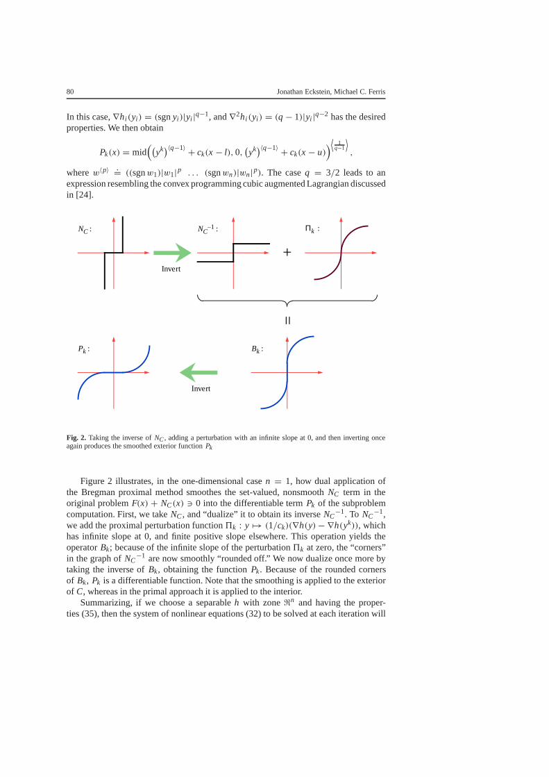
Πk :NC–1 :NC

:

Bk :Pk

:

Invert

Invert

Fig. 2. Taking the inverse ofNC, adding a perturbation with an infinite slope at 0, and then inverting onceagain produces the smoothed exterior functionPk

Figure 2 illustrates, in the one-dimensional casen = 1, how dual application ofthe Bregman proximal method smoothes the set-valued, nonsmoothNC term in theoriginal problemF(x) + NC(x) 3 0 into the differentiable termPk of the subproblemcomputation. First, we takeNC, and “dualize” it to obtain its inverseNC

−1. To NC−1,

we add the proximal perturbation function5k : y 7→ (1/ck)(∇h(y)− ∇h(yk)), whichhas infinite slope at 0, and finite positive slope elsewhere. This operation yields theoperatorBk; because of the infinite slope of the perturbation5k at zero, the “corners”in the graph ofNC

−1 are now smoothly “rounded off.” We now dualize once more bytaking the inverse ofBk, obtaining the functionPk. Because of the rounded cornersof Bk, Pk is a differentiable function. Note that the smoothing is applied to the exteriorof C, whereas in the primal approach it is applied to the interior.

Summarizing, if we choose a separableh with zone<n and having the proper-ties (35), then the system of nonlinear equations (32) to be solved at each iteration will


be differentiable. Note that the domain of definition of this system will be the sameasF’s, sincePk is finite and defined everywhere. Therefore, unlike the primal method,there is no need for stepsize guards, except for those required forF.

To make our dual procedure practical, we need only allow for approximate solutionof (32). In the following two theorems, we summarize the above development, incor-porating analysis of approximate forms of the iteration; however, the approximationcriteria take a somewhat strange form due to the subtleties of working in the dual. Welet dist(x,Y)

.= inf y∈Y ‖x− y‖.Theorem 2. Let F, l , andu describe a monotone NCP of the form (1), conforming to thehypothesis of Proposition 4, and possessing some solution. Fori = 1, . . . ,n, let hi bea Bregman function with zone<, and let{ck}∞k=0 ⊂ (0,∞) be bounded away from zero.

Suppose that the sequences{yk}∞k=0,{xk[1]}∞k=1

, {xk[2]}∞k=1⊂ <n and {δk}∞k=0 ⊂ [0,∞)

meet the conditions

∞∑k=0

ckδk max(1,∥∥yk

∥∥) <∞ (37)∥∥xk+1[1] − xk+1

[2]

∥∥ ≤ δk ∀ k ≥ 0 (38)

− F(xk+1

[1]

) = yk+1 = Pk(xk+1

[2]

) ∀ k ≥ 0, (39)

wherePk is defined as in (31). Thenyk → y∗ = −F(x∗), wherex∗ is some solutionto (1). All limit pointsx∞ of {xk

[1]} and {xk[2]} are also solutions of (1), withF(x∞) =

−y∗ = F(x∗). If im∇hi = < for all i , then such sequences are guaranteed to exist.

Proof. Invoking Proposition 4,TD = −F(−I ) + NC−1 is maximal monotone. Also

h(x).=∑n

i=0 hi (xi ) is a Bregman function with zone<n. We claim that{yk} confirmsto the recursion (26), where{ek}∞k=0 ⊂ <n is such that‖ek‖ ≤ δk for all k ≥ 0. Therecursion can be rewrittenAk(yk+1) + Bk(yk+1) 3 ek, whereAk and Bk are definedby (28)-(29). From (39), we have(xk+1

[1] ,−yk+1) ∈ F and(xk+1[2] , yk+1) ∈ Pk, which

yield (yk+1,−xk+1[1] ) ∈ Ak and(yk+1, xk+1

[2] ) ∈ Bk, courtesy of (28) andPk = Bk−1, as

established above. Settingek .= xk+1[1] − xk+1

[2] for all k ≥ 1, whence‖ek‖ ≤ δk by (38),

we haveAk(yk+1)+ Bk(yk+1) 3 ek, and the claim is established.Appealing to (37), (21) must hold with our choice of{ek}, and also (23). All the

hypotheses of Proposition 6 are thus satisfied, and so{yk} converges to a root ofTD + N<n = TD. The final statement follows from Proposition 7, even if we were torequireδk ≡ 0, so it only remains to show that all limit points of{xk

[1]} and{xk[2]} are

primal solutions.From (37) and{ck} being bounded away from zero,δk→ 0 andek→ 0. Therefore,

{xk[1]} and{xk

[2]} have the same limit points. Letx∞ be such that

xk[1], x

k[2] →k∈K

x∞

for some infinite setK ⊆ {0,1,2, . . . }. SinceF is continuous andyk = −F(xk[1]) for

all k ≥ 1, taking limits overk ∈ K yields y∗ = −F(x∞). From yk+1 = Pk(xk+1[2] ), we


also havexk+1[2] ∈ Bk(yk+1), and hence(

xk[2] +

1

ck

(∇h(yk)− ∇h

(yk+1)) , yk+1

)∈ NC

for all k ≥ 0. NC, being maximal monotone, is a closed set in<n×<n, while∇h mustbe continuous aty∗, and{ck} is bounded away from zero. So, taking limits overk ∈ Kyields(x∞, y∗) ∈ NC. Proposition 1 then gives thatx∞ must solve the primal problemF(x)+ NC(x) 3 0.

Theorem 3. In Theorem 2, sufficient conditions assuring (38)-(39) are

F(xk+1)+ Pk

(xk+1) = 0 (40)

yk+1 = Pk(xk+1) (41)

or

dist(

xk+1, F−1(− Pk(xk+1))) ≤ δk (42)

yk+1 = Pk(xk+1) (43)

or

dist(

xk+1, Bk(− F

(xk+1))) ≤ δk (44)

yk+1 = −F(xk+1), (45)

whereBk andPk are defined as in (29) and (31), respectively. If one of these alternativesholds at eachk ≥ 0, all limit points of{xk} solve the complementarity problem (1). IfF is continuously differentiable,∇2hi (yi ) exists and is positive for allyi 6= 0, whilelimyi→0∇2hi (yi ) = +∞, then the functionF + Pk on the left-hand side of (40) iscontinuously differentiable.

Proof. First consider the exact iteration (40)-(41). Then we can setxk+1[1] = xk+1

[2] = xk+1,and (38)-(39) will hold for anyδk ≥ 0. The continuous differentiability ofF+Pk followsfrom the discussion above.

Now consider (42)-(43). In this case, we letxk+1[2] = xk+1. SinceF and henceF−1

constitute maximal monotone operators, the setF−1(y) must be closed and convexfor every y ∈ <n (seee.g. [3]). Thus, (42) guarantees the existence of somexk+1

[1] ∈F−1(−Pk(xk+1)) such that‖xk+1

[1] − xk+1[2] ‖ ≤ δk. Thus, (38)-(39) can be satisfied.

The analysis of (44)-(45) is similar, except that we havexk+1[1] = xk+1, and (44)

guarantees the existence ofxk+1[2] .

Since eitherxk = xk[1] or xk = xk

[2] for everyk, the assertion about limit points of

{xk} follows from the limit point properties of{xk[1]} and{xk

[2]}


(40)-(41) constitute a generalized method of multipliers iteration for the comple-mentarity problem (1), and by appropriate choice ofh, the subproblem functionF+ Pk

of (40) can be made differentiable, ifF is differentiable. Of course, such an exact pro-cedure may not be practical. (44)-(45) is implementable in the general case and is likelyto be the most useful inexact version of (40)-(41). However, in special cases whereF−1

may be easily computed, (42)-(43) might also find application. To attempt to meet eitherset of approximate conditions, one would apply a standard iterative numerical methodto (40) until (42) or (44) holds.

The dual method set forth in Theorems 2 and 3 has several advantages over theprimal method of Section 3.1. Most crucially, the supplementary requirements P1 orP2 imposed onF in Theorem 1 may be dropped in place of the far weaker hypothesesof Proposition 4. Furthermore, the stepsize limit and ill-conditioning issues associatedwith the primal subproblemF(xk+1)+ ck

−1(∇h(xk+1)− ∇h(xk)) ≈ 0 do not arise inthe dual subproblemF(xk+1)+ Pk(xk+1) ≈ 0.

On the other hand, the dual method also has some disadvantages. First, the Jacobianof the primal subproblem takes the form∇F+ck

−1∇2h, and can be forced to be positivedefinite by requiring that∇2h be everywhere positive definite. The Jacobian∇F+∇Pkof the dual subproblem, however, is only guaranteed to be positivesemidefinite, unlessone requires∇F to be positive definite. Second, the primal method has the simple,residual-based approximation rule (32), whereas the dual method requires formulassuch as (42) or (44). Depending on the problem, these conditions might be difficult toverify. Finally, the dual method’s theory does not guarantee convergence of the primaliterates{xk}, {xk

[1]}, or {xk[2]}, but only makes assertions about limit points.

3.3. Primal-dual application to complementarity

The primal-dual method obtained by applying Proposition 6 toT = TPD= K [F, NC, I ]combines and improves upon the best theoretical features of the primal and dual methods.We now consider the basic recursion (20), as applied toT = TPD. First, we needa Bregman functionh on<n ×<n, which we construct via

h(x, y) = h(x)+n∑

i=1

hi (yi ), (46)

where thehi are as in the dual method, andh is a Bregman function with zoneS⊇ dom F.We partition the error vectorek of (20), which in this case lies in<n×<n, into subvectorsek

[1],ek[2] ∈ <n. Then the fundamental recursion (20), with iterateszk = (xk, yk),

Bregman functionh, and operatorTPD, takes the form

F(xk+1)+ yk+1 + 1

ck

(∇h(xk+1)−∇h

(xk)) = ek

[1] (47)

−xk+1 + NC−1(yk+1)+ 1

ck

(∇h(yk+1)−∇h

(yk)) 3 ek

[2], (48)

whereh(x) = ∑ni=1 hi (xi ), as before. If we setek

[2] ≡ 0, then (48) is equivalent to

Bk(yk+1) 3 xk+1, whereBk is defined as in (29) for the dual method. Using the prior


definition of Pk, this condition is in turn equivalent toyk+1 = Pk(xk+1), with Pk asin (31). Substituting this simple formula into (47), we obtain

F(xk+1)+ Pk

(xk+1)+ 1

ck

(∇h(xk+1)−∇h

(xk)) = ek

[1] .

At this point, application of Proposition 6 is straightforward.

Theorem 4. Let F be a continuous monotone function that is maximal when consideredas a monotone operator, with maximal open domainD⊆ <n. Suppose(F, l,u)describesa complementarity problem of the form (1), and that this problem has some solution.Let h be a Bregman function with (open) zoneS⊇ D, and let thehi , i = 1, . . . ,n beBregman functions with zone<. Let{ck}∞k=0 ⊂ (0,∞) be a sequence of positive scalarsbounded away from zero, and suppose that the sequences{xk}∞k=0 ⊂ S, {yk}∞k=0 ⊂ <n,and{dk}∞k=0 ⊂ <n conform to the recursion formulae

F(xk+1)+ 1

ck

(∇h(xk+1)−∇h

(xk))+ Pk

(xk+1) = dk (49)

yk+1 = Pk(xk+1) (50)

for all k ≥ 0, wherePk is defined by (31). Suppose also that∑∞

k=0 ck‖dk‖ <∞, while∑∞k=0 ck〈dk, xk〉 exists and is finite. Then{xk} converges to a solutionx∗ of the the

complementarity problem (1), andyk→−F(x∗). If im hi = < for all i andim h = <n,such sequences are guaranteed to exist. IfF is continuously differentiable and∇2hi (yi )

exists and is positive for allyi 6= 0, while limyi→0∇2hi (yi ) = +∞, then the functionF + ck

−1∇h + Pk in the equation system (49) is continuously differentiable. If, inaddition,∇2h is everywhere positive definite, then the Jacobian∇F+ ck

−1∇2h+∇Pk

of this function is everywhere positive definite.

Proof. Proposition 5 asserts thatTPD is maximal monotone. Letek = (dk,0) ∈ <n×<n

for all k ≥ 1. Then, similarly to the above discussion, (49)-(50)are equivalent to the Breg-man proximal recursion (20) with iterateszk = (xk, yk) and the Bregman functionh,which has zoneS× <n. Now,

∑∞k=0 ck‖dk‖ <∞ is equivalent to

∑∞k=0 ck‖ek‖ <∞,

and〈dk, xk〉 = 〈ek, (xk, yk)〉 = 〈ek, zk〉, so∑∞

k=1 ck〈ek, zk〉 exists and is finite.We can then apply Proposition 6 to give that{zk} = {(xk, yk)} converges to a root

z∗ = (x∗, y∗) ofTPD+ N

S×<n = TPD.

So,x∗ solves (1) andy∗ = −F(x∗) by the analysis of Section 2.2. The claim of existencefollows directly from Proposition 7. The remaining statements follow from argumentslike those of Section 3.2.

Note that the primal-dual method given as (49)-(50) requires neither the primalmethod’s restrictions P1 or P2 of Theorem 1, nor the dual method’s regularity conditionsof Proposition 4. The stepsize limit and ill-conditioning issues of the primal approachare also absent, because we choose the primal-space Bregman functionh to have


zone containing the domain ofF, as opposed to having zone intC. At the same time,the approximation criterion of (49) is based on simple measurement of a residual,as in the primal method. The Jacobian∇F + ck

−1∇2h + ∇Pk of the primal-dualsubproblem functionF+ck

−1∇h+ Pk combines the desirable existence/continuity andpositive definiteness features of the primal and dual methods. Unlike the dual method,convergence of the primal iterates{xk} is fully guaranteed.

Thus, the iteration (49)-(50) has all the theoretical advantages of the primal anddual approaches, and the disadvantages of neither. The three methods bear much thesame relationship as the proximal minimization algorithms, methods of multipliers,and proximal methods of multipliers presented for convex optimization in [30] (for thespecial caseh(x) = (1/2)‖x‖2) and later in [17] (for generalh). We therefore refer tothe dual method as a “method of multipliers,” and the primal-dual method as a “proximalmethod of multipliers.”

4. Computational results on the MCPLIB test suite

We conclude with some preliminary computational results for the proximal method ofmultipliers. We coded a version of the algorithm (49)-(50) in MATLAB, and used it tosolve the problems in the MCPLIB collection [14], exploiting the interface developedin [19]. We note that most of the problems in the collection do not satisfy the mono-tonicity condition (5) postulated in our theory. In fact, only the problemscycle andoptcont31 are definitely known to be monotone. However, for the method to bepractical, we believe it must robustly solve a large number of the problems from thisstandard test suite.

In our initial implementation, we set‖dk‖ < 10−6 for all k, that is, we solved (49)essentially exactly at all iterations. With later work, we intend to refine this approach,starting from a larger tolerance and gradually decreasing it. We choseh as in (36) withq = 3/2, and seth(x) = (1/2)x>Dx, D being a diagonal matrix determined via

Dii = 1.0

max(0.1∥∥∇Fii (x0)

∥∥,10.0) .

This choice corresponds to standard problem scaling mechanisms that have provensuccessful in [10,15]. In the interest of further improving scaling, we also define thefunction Pk slightly differently from (31). Instead, we usePk(x) = P(x, yk; ck) where

P(x, y; c) .= (∇h)−1

mid

∇h(y)+ cD−1(x− l)∇h(0)

∇h(y)+ cD−1(x− u)

, (51)

D being the diagonal matrix defined above. This change corresponds to a simple rescal-ing of the overall Bregman functionh of (46).

By way of illustration, consider the special case of minimization over the nonnegativeorthant, where we haveF = ∇ f for some differentiable convex functionf , l = 0, and


u = +∞. Then the version of (49)-(50) we implemented would correspond to thefollowing cubic augmented Lagrangian method, with a quadratic proximal term:

xk+1 = arg minx∈<n

{f(x)+ 1

2ck

(x− xk

)>D(x− xk

)+ 13

n∑j=1

max

{[√yk

j + ckx jD j j

]3,0

}}yk+1

j = max

(√yk

j +ckxk+1

jD j j

,0

)2

.

The initial valuesx0 of the primal variables are specified in the MCPLIB testsuite [14]. For the initial multipliers, we used the formula

y0 ={

P(x0,−F

(x0) ; c0

),

∥∥P(x0,−F

(x0) ; c0

) ∥∥ ≥ 10−6

−F(x0), otherwise,

whereP is defined by (51).The major work involved in each step of the algorithm is in solving the system of

nonlinear equations (49), for which we use a simple backtracking variant of Newton’smethod. We start by computing a “pure” Newton step for (49), withdk replaced by zero.If this step does not yield a reduction in the residual of (49), we repeatedly halve thestep size until a reduction is obtained, or the step is less than 1/1000th of its originalmagnitude. In the former case, we then attempt another Newton step, repeating theprocess until the residual of (49) falls below 10−6. We then update the multiplier vectorvia (50), and check the global residualrk

.= ‖F(xk)+ yk‖. If rk < 10−6, we successfullyterminate. Otherwise, ifk < 100, we loop, incrementk, and execute another “outer”iteration. Ifk ≥ 100 we quit and declare failure.

When the Newton line search fails, that is, a reduction of the step by a factor of1/1024 fails to yield any improvement in the residual of (49), we update the proximalstepsize parameterck. In fact, we separately maintain a primalck (“pck”) and a dualck(“dck”), corresponding to the usage ofck in the equations (49) and (31)/(51), respectively.Allowing for additional rescaling ofh, the convergence theory above stipulates that pckand dck be held in a fixed ratio to one another throughout the algorithm. In practice, weallow a limited number of independent adjustments of these two parameters. Assumingmonotonicity of F, our convergence theory applies after the last such independentadjustment.

We start by setting pc0 = max{10, ‖x0‖} and dc0 = 10. Upon failure of theline search, pck is reduced by a factor of 10 and dck is set to 1. After successfulsolution of (49) to the tolerance of 10−6, both pck and dck are multiplied by 1.05;this adjustment is consistent with our theory and also with standard techniques foraccelerating convergence of proximal methods. We then calculateyk+1, and if∥∥xk+1 − xk

∥∥ > 100∥∥yk+1 − yk

∥∥,dck is doubled, whereas if

100∥∥xk+1 − xk

∥∥ < ∥∥yk+1 − yk∥∥,

then dck = ‖yk‖.


Table 1.Primal-dual smooth multiplier method applied to MCPLIB problems (part 1)

Problem Newton Updates Updates Primal(Starting Point) Iterations Steps of pck of dck Residual

bertsekas (1) 15 40 0 0 5.4× 10−7

bertsekas (2) 15 47 0 0 6.3× 10−7

bertsekas (3) 6 59 0 0 1.2× 10−8

billups (1) 47 350 3 21 4.9× 10−7

choi (1) 5 8 0 1 9.3× 10−7

colvdual (1) 9 29 1 1 7.2× 10−8

colvdual (2) 7 36 0 0 2.4× 10−7

colvnlp (1) 9 28 1 1 7.4× 10−8

colvnlp (2) 7 25 0 0 2.3× 10−7

cycle (1) 4 11 0 0 8.3× 10−7

ehl_kost (1) 4 15 0 0 5.5× 10−7

ehl_kost (2) 4 15 0 0 5.5× 10−7

ehl_kost (3) 4 15 0 0 5.5× 10−7

explcp (1) 6 21 0 0 5.6× 10−7

freebert (1) 15 39 0 0 4.0× 10−7

freebert (2) 9 24 0 0 8.4× 10−7

freebert (3) 15 39 0 0 3.7× 10−7

freebert (4) 15 40 0 0 5.4× 10−7

freebert (5) 9 24 0 0 8.4× 10−7

freebert (6) 15 40 0 0 5.0× 10−7

gafni (1) 9 23 0 0 2.7× 10−7

gafni (2) 9 26 0 0 3.0× 10−7

gafni (3) 9 28 0 0 3.3× 10−7

hanskoop (1) 5 30 0 0 1.4× 10−7

hanskoop (2) 11 108 1 1 8.0× 10−7

hanskoop (3) 5 17 0 0 1.1× 10−7

hanskoop (4) 5 26 0 0 1.4× 10−7

hanskoop (5) 11 78 1 1 7.0× 10−7

hydroc06 (1) 5 9 0 0 5.8× 10−7

hydroc20 (1) failed

josephy (1) 13 105 2 2 6.3× 10−7

josephy (2) 8 90 1 1 5.6× 10−8

josephy (3) 7 138 1 1 8.7× 10−7

josephy (4) 5 14 0 0 8.9× 10−9

josephy (5) 4 10 0 0 4.4× 10−7

josephy (6) 8 166 1 1 1.9× 10−7

kojshin (1) 56 248 3 3 5.3× 10−7

kojshin (2) 9 151 1 1 8.4× 10−8

kojshin (3) 43 357 4 4 8.6× 10−7

kojshin (4) 19 214 2 2 8.4× 10−7

kojshin (5) 20 227 2 2 5.5× 10−7

kojshin (6) 52 391 3 3 7.6× 10−7

mathinum (1) 5 9 0 0 4.1× 10−8

mathinum (2) 5 8 0 0 1.3× 10−8

mathinum (3) 5 13 0 0 2.4× 10−8

mathinum (4) 5 9 0 0 4.5× 10−8


Table 2.Primal-dual smooth multiplier method applied to MCPLIB problems (part 2)

Problem Newton Updates Updates Primal(Starting Point) Iterations Steps of pck of dck Residual

mathisum (1) 4 9 0 0 2.5× 10−7

mathisum (2) 5 11 0 0 1.9× 10−8

mathisum (3) 5 19 0 0 3.9× 10−8

mathisum (4) 4 8 0 0 9.8× 10−7

methan08 (1) 4 7 0 1 2.9× 10−7

nash (1) 5 10 0 0 1.2× 10−8

nash (2) 4 9 0 0 5.2× 10−8

opt_cont31 (1) 6 85 0 0 4.7× 10−7

pies (1) 7 29 1 1 6.5× 10−7

pgvon105 (1) failedpgvon106 (1) failed

powell (1) 4 12 0 0 4.2× 10−7

powell (2) 6 21 0 0 1.0× 10−7

powell (3) 14 176 2 2 2.8× 10−7

powell (4) 6 21 0 0 8.2× 10−8

powell_mcp (1) 5 10 0 0 2.2× 10−7

powell_mcp (2) 5 10 0 0 3.8× 10−7

powell_mcp (3) 5 14 0 1 1.6× 10−7

powell_mcp (4) 5 13 0 0 6.7× 10−7

scarfanum (1) 6 24 0 0 3.0× 10−7

scarfanum (2) 6 28 0 0 3.0× 10−7

scarfanum (3) 7 28 0 0 1.5× 10−7

scarfasum (1) 6 25 0 0 1.4× 10−7

scarfasum (2) 6 21 0 0 1.4× 10−7

scarfasum (3) 10 36 0 0 2.9× 10−7

scarfbnum (1) 43 133 0 0 5.9× 10−7

scarfbnum (2) 89 393 0 21 9.0× 10−7

scarfbsum (1) 18 81 0 0 5.7× 10−7

scarfbsum (2) 18 66 0 0 5.8× 10−7

sppe (1) 6 21 0 0 5.8× 10−8

sppe (2) 5 22 0 0 6.9× 10−9

tobin (1) 6 30 0 0 3.5× 10−8

tobin (2) 6 47 0 0 3.3× 10−8

Tables 1 and 2 summarize our computational results. “Iterations” is the total numberof “outer” iterations, that is, the value ofk necessary to obtainrk < 10−6. “Newtonsteps” is the total number of Newton steps taken, accumulated over all outer iterations.We also report the number of times that pck and dck are updated independently of oneanother; these counts do not include the simultaneous multiplications by 1.05. Note thatthere were no independent updates required for the two guaranteed monotone problems,as our convergence theory would suggest. For the remaining problems, independentupdates were infrequent. Since our implementation is preliminary and MATLAB is aninterpreted language, we do not list run times. The “primal residual” column gives thefinal value of‖xk −mid

(l, xk − F(xk),u

) ‖.


As can be seen from the tables, and by comparison with the results in [2], thealgorithm is fairly robust. For all but 3 of the 79 instance/starting point combinationsattempted, it terminates within 100 iterations with a primal residual of 10−6 or less,indicating convergence to a solution. Two of the failures were for thepgvon10*problems; since these problems are known to be poorly defined at the solution, we donot consider these failures to be a serious liability. The other failure, onhydroc20 ,seems to be due to convergence difficulties in the multiplier space.Hydroc20 containsa large number of nonlinear equations, and we speculate that (36) withq = 3/2 maynot be an ideal penalty kernel to use in such cases.

Acknowledgements.The authors also wish to thank an anonymous referee for suggestions on streamliningsome of the analysis.

References

1. Attouch, H., Théra, M. (1996): A general duality principle for the sum of two operators. J. Convex Anal.3, 1–24

2. Billups, S.C., Dirkse, S.P., Ferris, M.C. (1997): A comparison of large scale mixed complementarityproblem solvers. Comput. Optim. Appl.7, 3–25

3. Brézis, H. (1973): Opérateurs Maximaux Monotones et Semi-Groupes de Contractions dans les Espacesde Hilbert. North-Holland, Amsterdam

4. Bruck, R.E. (1975): An iterative solution of a variational inequality for certain monotone operators inHilbert space. Bull. Am. Math. Soc.81, 890–892

5. Burachik, R.S., Iusem, A.N. (1995): A generalized proximal point algorithm for the nonlinear comple-mentarity problem. Working paper, Instituto de Matemática Pura e Aplicada, Rio de Janeiro

6. Burachik, R.S., Iusem, A.N. (1998): A generalized proximal point algorithm for the variational inequalityproblem in a Hilbert space. SIAM J. Optim.8, 197–216

7. Burachik, R.S., Iusem, A.N., Svaiter, B.F. (1997): Enlargement of monotone operators with applicationsto variational inequalities. Set-Valued Anal.5, 159–180

8. Censor, Y., Iusem, A.N., Zenios, S.A. (1998): An interior-point method with Bregman functions for thevariational inequality problem with paramonotone operators. Math. Program.81, 373–400

9. Censor, Y., Zenios, S.A. (1992): The proximal minimization algorithm withD-functions. J. Optim.Theory Appl.73, 451–464

10. Chen, C., Mangasarian, O.L. (1995): Smoothing methods for convex inequalities and linear complemen-tarity problems. Math. Program.78, 51–70

11. Chen, C., Mangasarian, O.L. (1996): A class of smoothing functions for nonlinear and mixed comple-mentarity problems. Comput. Optim. Appl.5, 97–138

12. Chen, G., Teboulle, M. (1993): A convergence analysis of proximal-like minimization algorithms usingBregman functions. SIAM J. Optim.3, 538–543

13. De Pierro, A.R., Iusem, A.N. (1986): A relaxed version of Bregman’s method for convex programming.J. Optim. Theory Appl.51, 421–440

14. Dirkse, S.P., Ferris, M.C. (1995): MCPLIB: A collection of nonlinear mixed complementarity problems.Optim. Methods Software5, 319–345

15. Dirkse, S.P., Ferris, M.C. (1995): The PATH solver: A non-monotone stabilization scheme for mixedcomplementarity problems. Optim. Methods Software5, 123–156

16. Eckstein, J. (1989): Splitting Methods for Monotone Operators, with Applications to Parallel Opti-mization. PhD thesis. Massachusetts Institute of Technology, Cambridge, MA, 1989. Also available asReport LIDS-TH-1877, Laboratory for Information and Decision Systems, Massachusetts Institute ofTechnology, Cambridge, MA, 1989

17. Eckstein, J. (1993): Nonlinear proximal point algorithms using Bregman functions, with applications toconvex programming. Math. Oper. Res.18, 202–226

18. Eckstein, J. (1998): Approximate iterations in Bregman-function-based proximal algorithms. Math.Program.83, 113–124

90 Jonathan Eckstein et al.: Smooth methods of multipliers for complementarity problems

19. Ferris, M.C., Rutherford, T.F. (1996): Accessing realistic complementarity problems within Matlab. In:Di Pillo, G., Giannessi, F., eds., Proceedings of Nonlinear Optimization and Applications Workshop,Erice, June 1995. Plenum Press, New York

20. Fukushima, M. (1996): The primal Douglas-Rachford splitting algorithm for a class of monotone map-pings with application to the traffic equilibrium problem. Math. Program.72, 1–15

21. Gabay, D. (1983): Applications of the method of multipliers to variational inequalities. In: Fortin, M.,Glowinski, R., eds., Augmented Lagrangian Methods: Applications to the Solution of Boundary ValueProblems. North-Holland, Amsterdam

22. Gabriel, S.A., Moré, J.J. (1997): Smoothing of mixed complementarity problems. In: Ferris, M.C., Pang,J.S., eds., Complementarity and Variational Problems: State of the Art. SIAM Publications, Philadelphia

23. Kabbadj, S. (1994): Methodes Proximales Entropiques. Doctoral thesis. Université de Montpellier II –Sciences et Techniques du Languedoc, Montpellier, France

24. Kiwiel, K.C. (1996): On the twice differentiable cubic augmented Lagrangian. J. Optim. Theory Appl.88, 233–236

25. Luo, Z.-Q., Tseng, P. (1993): Error bounds and convergence analysis of feasible descent methods:A general approach. Ann. Oper. Res.46, 157–178

26. Minty, G.J. (1962): Monotone (nonlinear) operators in Hilbert space. Duke Math. J.29, 341–34627. Mosco, U. (1972): Dual variational inequalities. J. Math. Anal. Appl.40, 202–20628. Rockafellar, R.T., (1970): Convex Analysis. Princeton University Press, Princeton, NJ29. Rockafellar, R.T. (1970): On the maximality of sums of nonlinear monotone operators. Trans. Am. Math.

Soc.149, 75–8830. Rockafellar, R.T. (1976): Augmented Lagrangians and applications of the proximal point algorithm in

convex programming. Math. Oper. Res.1, 97–11631. Rockafellar, R.T. (1976): Monotone operators and the proximal point algorithm. SIAM J. Control Optim.

14, 877–89832. Rockafellar, R.T., Wets, R.J.-B. (1998): Variational Analysis. Springer33. Teboulle, M. (1992): Entropic proximal mappings with applications to nonlinear programming. Math.

Oper. Res.17, 670–690

Smooth methods of multipliers for complementarity problems

Documents

Transcript of Smooth methods of multipliers for complementarity problems