JOURNAL OF PURE AND APPLIED ALGEBRA

Journal of Pure and Applied Algebra 122 (1997) 209-241

Smooth points of 3’0r(T)

A.V. Geramitaa*b,*,l, M. Puccic,2, Y.S. Shinds3

a Queen s University, Kingston, Canada K7L 3N6

b University of Genoa, Genova, Italy

’ University of Perugia, Perugia, Italy

d Sunmoon University. Choongnam, South Korea

Communicated by T. Hibi; received 10 July 1996

Dedicated to the memory of Professor Hideyuki Matsumura

Abstract

In this paper we investigate some relationships between codimension 2 Cohen-Macaulay graded rings and codimension three Artinian Gorenstein graded rings and use these to make some comments about the classifying spaces of such Gorenstein algebras having a fixed Hilbert function. 0 1997 Elsevier Science B.V.

AMS ClassiJication: 13A02, 13C13, 14A05, 14M05, 14M12

0. Introduction

Iarrobino and Kanev [15] have introduced interesting parameter spaces for arti-

nian graded Gorenstein algebras, and have raised several fascinating questions about

these objects. A fundamental set of problems concerns the dimension and smoothness

of these parameter spaces.

This paper deals with these particular problems in the case where the Gorenstein

algebras in question are graded quotients of k[xo, x1, x2], i.e. the artinian Gorenstein

algebras of embedding codimension 13. In this case there are many works on this

much studied class of rings - results which grow out of the Buchsbaum-Eisenbud

*Corresponding author.

’ Supported, in part, by a grant from the NSERC of Canada.

‘This author would like to thank the Mathematics and Statistics Department of Queen’s University for

hospitality during the preparation of this paper.

3 Current address: Sungshin Women’s University, Seoul, South Korea. This paper was supported by the

Grants for Professors of Sungshin Women’s University in 1997. This author would also like to thank the

Mathematics and Statistics Department of Queen’s University for kind hospitality during the preparation

of this work.

0022-4049/97/$17.00 0 1997 Elsevier Science B.V. All rights reserved

PI1 SOO22-4049(97)000052-2

210 A. V. Geramita et al. /Journal of Pure and Applied Algebra 122 (I 997) 209 -241

structure theorem for such algebras [4]. In fact, our work is a natural outgrowth of an

earlier work in this area by Diesel [9].

We begin by briefly reviewing the fundamentals of the Iarrobino-Kanev classifying

spaces and set up the notation we shall need and define the problem we study.

We then pass to the study of the Hilbert function of artinian quotients of k[xo, x1] and introduce the notion of the alignment character of such a Hilbert function. This

character is our basic tool for describing the dimensions of the parameter spaces

mentioned above. We also review and recast the “numerical” study of codimension 2

arithmetically CohenMacaulay (henceforth ACM) algebras, in terms of the align-

ment character.

We then relate this “codimension 2 ACM” discussion to the “codimension 3 Goren-

stein” case and review (and recast, in terms of the alignment character) the analogous

numerical facts for these Gorenstein rings. The key ingredients here are the character-

ization by Stanley [22] of the Hilbert functions of such Gorenstein algebras and

a construction method of Harima [14] for a special class of such algebras. A theorem

of Kustin-Ulrich [16] on the resolution of the square of an ideal defining such an

algebra is also reviewed.

We then state our conjectures about the dimensions of the Iarrobino-Kanev

classifying spaces, verifying them for several important special cases. These extend

analogous results of Iarrobino-Kanev in the codimension 3 case.

1. The classifying spaces Gor(T) and %or(T)

Since the classifying spaces Gor( T) and ??‘or( T) are not so well known, we shall take

some time to recall a few basic ideas. For more details (including proofs of unsup-

ported statements) one can consult either the paper of Iarrobino and Kanev [15] or

the expository article [lo].

Let R = k[xo,..., x,] (k an algebraically closed field of characteristic 0) and let

I c R be a homogeneous ideal for which A = R/I = @Ai is a graded Gorenstein

artinian k-algebra with socle degree j (i.e. for which dimk Aj = 1 and dimk Aj+, = 0 for

all t > 0).

Recall that Macaulay exhibited a bijective correspondence between such graded

Gorenstein artinian quotients of R having socle degreej and the projective space P(Sj)

where S = k [yo, . . . , y,,].

The correspondence can be effected by the “apolar” duality of Macaulay, i.e. we

consider the elements of the ring R as partial differential operators which operate on

the elements of the ring S. This action turns S into a (non-finitely generated)

R-module. Having said this, the Macaulay correspondence can be described as

follows:

if FESS and I = arm,(F) then A = R/I is the corresponding (graded)

Gorenstein artinian algebra with socle degree j.

A. V. Geramita et al. 1 Journal of Pure and Applied Algebra 122 (I 997) 209-241 211

Once we observe that anna = anna for any i E k*, the correspondence with

P(Sj) is then clear.

A

We let H(A, t) := dim, A, = h, denote the Hilbert function of the Gorenstein ring

above. If we continue to letj denote the socle degree of A then it is well known that

(A,) ho = hj = 1;

(B,) hi = hj_i for all i = 0, . . . ,j;

(Cl) hi I min{(‘:“), (jPL+“)} for all i = 0, . . . , j.

The vector

is then referred to as the h-vector of the ring A.

Now for fixed n and j one can consider arbitrary sequences of positive integers

T = (h@hi,&, . . . , hi_ 1, hj) which satisfy (A,), (B,), and (C,) above. We shall call such

a sequence a symmetric sequence of length j.

Apart from a theorem of Serre for the case n = 1 (which says that a Gorenstein

quotient of k[xo, xl] is a complete intersection) and a theorem of Stanley for the case

n = 2 (which we shall describe below ~ Theorem 2.11) little is known about which

symmetric sequences of length j can be the h-vector of a Gorenstein graded k-algebra

(but see [2, 31).

Now let Ti = (~,,,a~, . . . , Uj_ 1, Uj) and Tz = (b,, bl, . . . , bj_ 1, hj) be two symmetric

sequences of length j. We say that T1 I T2 if ai I bi for all i = 0, 1, . . . ,,j, and that

T1 < T, if T, I T2 and ai < bi for at least one index i.

Notice that for a fixed n and j there are only a finite number of possible symmetric

sequences of length j and that there is a unique minimal such sequence, namely

Y

j + 1.umes

and a unique maximal such sequence, namely

Tgix = 1 n + 1 (, ,(n~2),(n~3),...,(n~3).(n~2),n+L~).

Definition 1.1. Let T be a symmetric sequence of lengthj. We denote by

(9

and

Gor( 5 T) = {[F] E P(Sj)Jif I = annR(F) and A = R/I then h(A) I T)

(ii) Gor(T) = Gor(l T)\(T,TGor(Tf)).

Now, if F is a form of degree j in S and I is its annihilator in R, it is known (via

Macaulay’s inverse systems, see e.g. [ 10,151 for details) that the Hilbert function of the

Gorenstein ring R/I is the same as that of the R-submodule of S generated by F. We

can figure out the dimensions of the graded pieces of this submodule by calculating

212 A. V. Geramita et al. /Journal of Pure and Applied Algebra 122 (1997) 209-241

the ranks of various catalecticant matrices. The following simple example will suffice to give the ideas.

Example 1.2. Let F = yz + (y,y,)* + y: in k[y,, y,, y2]. The R-submodule of S gen- erated by F is:

By symmetry, it will be enough to calculate dimk RIF and dimk R2F. Now

xoF = WY,(F) = 4~; + ~YOY:,

XIF = WYI(F) = ~Y;Y,,

x2F = a/~?y,(F) = 4~;.

So, dim, RIF is the rank of the 3 x 10 matrix below (whose rows are indexed by x0, x1, x2 - the monomials of degree 1 in R - and whose columns are indexed by the

ordered lexicographically); monomials of degree 3 in S

L

4002000

0200000

0000000 0 0

0 0

0 I

0.

0 0 4

This matrix has rank 3. As for the dimension of R2F, we first calculate:

x;F = &(F) = 12~; + 2y:, 0 0

xox,F = &(F) = 4~0~1,

xox2F = &(F) = 0, 2

x:F = &(r, = 2y& 1 1

xlx2F = &(F)=O, 1 2

x$F = &(F) = 1’44, 2 2

A. V. Geramita et al. /Journal of Pure and Applied Algebra 122 (1997) 209-241 213

and then find the rank of the 6 x 6 matrix

‘12 0 0 2 0 0

0 4000 0

0 0000 0

2 0000 0

000000

,o 0 0 0 0 12

(whose rows are indexed by the monomials of degree 2 in R and whose columns are

indexed by the monomials of degree 2 in S-ordered lexicographically). Since this last matrix has rank 4 we obtain: if I = anna and A = R/Z, the

h-vector of A is (1, 3, 4, 3, 1).

The matrices of this example are two of the various catalecticant matrices we can associate to F. They are usually referred to as CatF(l, 3) and CatF(2, 2) respectively.

This example is easily abstracted as follows: we can form a determinantal sub-

scheme of p(Sj), called %r( I T), by imposing the appropriate rank conditions on the catalecticant matrices associated to the generic form of degree j in S. Moreover, by considering the scheme-theoretic difference, we can also define the schemes gor(T).

Notice that, with these definitions, we have

Gor( I T) = got-( 5 T)‘ed and Gor(T) = Yor(T)“d.

Thus, both Gor( I T) and Gor(T) are reduced algebraic varieties. In particular, the Gor( I T) are all closed subvarieties of p(Sj) and, if T # T,f,‘i,,, Gor(T) is open in

p(sj).

Example 1.3. (See also [lo]). (1) For fixed n and j we have

Gor( 5 T$)“) = Gor(T,!$,) = Vj(P”) L I,

where vj(~n) is the Veronese embedding of P” in p(Sj). (This is SO because it is easy to prove that A = R/I has h(A) I T,$,, if and only if I = arm,(F) where F = Lj (L a linear form in S,).) Pucci has recently shown that Sor(T,!&) = Vj(pn), i.e. that the scheme 3or(TEjn) is a reduced scheme! This will be the subject of another work.

(2) Fix n and j and let Tf’ = (1,2,2 , . . . ,2,2,1). One can show that in this case Gor( < T$“‘) is the secant (line) variety to vj(pn) in p(Sj), denoted Secl(vj(p”)). Notice that this is a singular variety in p(Sj) whose singular points are precisely Gor(T,$). I.e. in this case the points of Gor(Tp’) are the smooth points of Gor( I T$“‘).

(3) A more elaborate example is provided by considering all symmetric sequences of length 4 which can be the h-vector of a Gorenstein quotient of k[x,,, x1, x2] (see Theorem 2.11).

214 A. V. Geramita et al. /Journal qf’ Pure and Applied A Igebra 122 (1997) 209-241

In this case the sequences are linearly ordered by

TI = (1, 3,633, 1), Tz = (1, 3,5,3, l), T3 = (1,3,4, 3, l),

Th=(l,3,3,3,1), Tg=(1,2,2,2,1), T,=(l,l,l,l,l).

We have already commented on Gor(T,) and Gor( I T,).

Now (see [lo]) for details we have:

Gor( 5 T4) 2 Sec,(v,(P”))

(the variety of secant planes to (vq(P2)), a variety of dimension 8);

Gor( I T3) 3 Sec3(v4(P2))

(the variety of secant P3’s to (vq(P2)), a variety of dimension 11):

Gor( 5 T,) 2 Sec,(v,(P2))

(the variety of secant P4’s to (v4(P2)), a variety of dimension 13, one of the

deficient secant varieties to v4(P2)).

In order to describe the schemes Yor( < Ti) (for the Ti above) let

F = V;: + bYiY1 + cY:Y2 + dY;y: + (‘YiYlY2 +fyiyZ + SYOY? + hYoY:Y,

+ kyoY,y; + ~Y,Y; + my: + PY:Y, + ~Y,Y; + SY;

be a general form of degree 4 in S4 (S = k[yo, yl, y2]).

The two relevant catalecticant matrices are:

ahcdefghkl

d e g k k m p q

cefhklpqrs

and

ahcdef

bdeghk

B= dghmpq

.

ehkpqr

fklqrs

Note. For simplicity in the exposition (and since we are assuming that the character-

istic of k is 0) in writing these catalecticants we have suppressed the coefficients that

arise from differentiation. That this creates no problem, in characteristic 0, is ex-

plained in [IO, Section 91.

A. V. Geramita et al. /Journal of Pure and Applied Algebra 122 (1997) 209-241 215

If we let Z,(M) be the ideal generated by the t x t minors of the matrix M, then:

%r( I T2) is defined by Z,(B), %r( I T,) is defined by Z,(B),

Yor( I T,) is defined by Z,(B), %or( I T,) is defined by Z,(B) + Z,(A),

Bor(T6) is defined by Z,(B) + Z,(A).

In view of Pucci’s recent work, cited above, Z,(B) = Z,(A) is the defining ideal of

r4(p2). So, %r(T,) = Gor(T,) = v,(P2).

Since Z,(B) = det B (known to be the irreducible polynomial of degree 6 which

defines Sec,(v,(iFD2))), we also have

Gor( I T,) = Yor( I T2) = &c,(v,(~~)).

There are many interesting questions one can ask about these classifying spaces and

the first significant steps towards understanding them have been taken by Iarrobino

and Kanev in [ 151 and Diesel in [9]. It is a well-known problem to try and determine

even when Gor(T) # (b!

Iarrobino and Kanev [15, Theorem 2.51 have proved a wonderful theorem which

gives the dimension of the tangent space to the scheme Sor(T) at any of its closed

points. More precisely (and with the notation of this section):

Theorem 1.4 (Iarrobino and Kanev [lS]). Let F ES~ and let Z = arm,(F) 5 R. Let

T = h(A) be the h-vector of the Gorenstein ring A = R/Z and let YF he the tangent space

to the scheme %or(T) at the point [F]. Then

dimkYp + 1 = dim,(R/Z’)j.

Thus, in view of this theorem, it is important to be able to calculate the dimension,

as vector space, of the degree j piece of the ideal 1’.

We propose to do this for some Z c k[xo, x1, x2], i.e. for some codimension 3

Gorenstein ideals. Our methods involve making a detailed study of certain codimen-

sion 2 Cohen-Macaulay ideals and using these results (with liaison) to say something

about the codimension 3 Gorenstein case.

2. Hilbert functions of codim 2 Cohen-Macaulay and codim 3 Gorenstein rings

It is well-known that the study of Hilbert functions of arithmetically Cohen-

Macaulay quotients, by height two ideals of k[xo,xI, . . . ,xn], is equivalent to the

study of Hilbert functions of quotients of k[xo, xl] by ideals Z having radical (x0, .~r).

If A = k[xo, x11/Z = OAi is such a k-algebra and if we let H(A, t) = dimkA, = a,,

then the (infinite) sequence of integers

a,,a,, . . . . O,O, . .

216 A. V. Geramita et al. /Journal of Pure and Applied Algebra 122 (1997) 209-241

is the Hilbert function of the ring A. (Since fi = (x0, x1), the Hilbert function is eventually 0.)

We denote by (T = o(l) (or o(A)) the least integer for which

H(A, a) = 0 and H(A, CJ - 1) # 0.

It follows that H(A, t) = 0 for all t 2 CJ. The least integer f for which I, # 0 is denoted

41) (or 44). With this notation, the vector of positive integers

contains all information on the Hilbert function of A. This is the h-vector of the ring A.

It is well-known (see e.g. [7]) that the entries of the h-vector of A (as above) satisfy: (A) ai I i + 1 for all i, with equality o 0 I i I ~(1) - 1;

(B) ai 2 Ui+l for CC(Z) - 1 I i.

Furthermore, any vector of positive integers which satisfies (A) and (B) is the h-vector of some artinian quotient of k[xo, x1].

This permits us to discuss the vectors of this type as Hilbert functions without ever specifying any ring! Consequently, if T = (1, a1,u2, . . . ,a,) is a vector of positive integers satisfying (A) and (B) we can speak of a(T) and o(T). Moreover, given such a T, the vector T’ made from the positive integers in the sequence

U 1 - 1, a, - 1, . . ..a. - 1

also satisfies (A) and (B), and thus we can write

T’ = (l,bl, . . . ,b,,) with n’ 5 n - 1.

If n’ 2 1 we can repeat the process. In fact, the process can be repeated exactly cc(T) - 1 times and the resulting sequence of integers - o(T), a(T’), . . . - is a strictly decreasing family of integers. If we reorder these integers in increasing order we obtain, what we shall call, the alignment character of T.

Example 2.1. Let T = (1,2,3,4,3,3, 1). Then a(T) = 4 and a(T) = 7. Now T’ = (1,2, 3,2,2) and a(T’) = 5. Repeating we get T” = (1,2, 1, 1) and o(T”) = 4. Repeating the procedure once again we get T”’ = (1) and CJ(T”‘) = 1. Thus, the alignment character of T is (1, 4, 5, 7).

If we are given an alignment character (d,, . . . , d,), the following procedure shows how to construct a vector T = (1, tl, . , td,_ 1) satisfying (A) and (B) and having alignment character (d,, . . . , d,).

A. V. Geramita et al. J Journal of Pure and Applied Algebra 122 (1997) 209-241 217

Let cd denote the infinite sequence consisting of d l’s followed by 0’s. Write down

the sequences gdl, . , ad, (successively shifting them to the left) and add, i.e.

cdl : 1 1 ... 1 0 --+

& : 11 ... 10 4

cd, : 1 1 . . . 1 0 +

T : 1 2 t2

One verifies that

ti = 5 cTd~(,j + i - m). j=l

Thus, there is a l-l correspondence between vectors of positive integers satisfying

(A) and (B) and alignment characters.

Now let X = {PI, . . . . Ps} be a set of s (distinct) points in P2 where

Pi++ fJi = (Lil, Liz) c /c[x~,x~,x~] = R (the Lij linear forms). Then

I = Z(X) = pin ... nps

and A = R/I = OAi is the homogeneous coordinate ring of X.

The Hilbert function of X (or of A = R/I) is the function

H(A, t) = H,(t) := dimk A,.

It is well-known (and easy to prove) that if L is a linear form which describes a line

in P2 which misses all the points of X then z is not a divisor of zero in the ring A. We

can, by making a linear change of variables if necessary, assume that L = x2. Then if

we write B = A/LA, we have B N k[xO, xJ/J where fi = (x,, x1) and

H(B, t) = H(A, t) - H(A, t - l):= dH(A, t)

is thejrst dijizrence of the Hilbert function of A (or X). (Higher differences are formed

in the obvious way.)

Since B N k[x,, x,1/J, $ = ( x0, x1), we can (and will) speak of the alignment

character of the h-vector of B. If no confusion can occur, we call it also the alignment

character of Hx. We also write CC(X) and @X)for cc(B) and g(B).

We now explain where the name “alignment character” comes from.

Proposition 2.2. Let H, be the Hilbertfunction of a set of s distinct points in P2 and let

(dl,d2, . . . ,d,) be the alignment character of Hx.

218 A. V. Geramita et al. /Journal of Pure and Applied Algebra I22 (1997) 209-241

There is another set, V, of s points in P2, with Hx = HY and such that the points of

V are distributed among m distinct lines lL1, L2, . , II, with:

dl points on the line L1;

d2 points on the line L2;

d, points on the line L,.

Proof. See [ll]. 0

Example 2.3. It is very easy to show that 8 points, X, on an irreducible conic in P2

have Hilbert function:

Hw:l 3 5 7 8 8 ...

i.e.

AH,:1 2 2 2 1 0 ...

A line of P2 contains none, one or two points of X.

Nevertheless, the alignment character of HX is (3, 5) and the following 8 points, W,

l eo

0.0..

have H, = HX.

With this proposition in mind, Roberts and Roitman [20] introduced the following

definition:

Definition 2.4. A k-configuration is a finite set X of points in P2 which satisfies the

following conditions:

there exist integers 1 5 dl < ... < d,, and subsets Xi, . . ,X, of X, and distinct

lines LL,, . . . , U., E P2 such that:

(1) X = uy! 1 Xi;

(2) [Xi] =di and Xi c [Li for each i = l,...,m, and;

(3) Li (1 < i I m) does not contain any points of Xj for all j < i. In this case, the k-configuration in P2 is said to be of type (d,, . . . ,d,).

It is easy to show that if X is a k-configuration of type (d,, . . . , d,) and if we

construct the vector T satisfying (A) and (B) above and which corresponds to the

alignment character (d,, , d,), then

T = (dH(X, 0), dH(X, l), . . . , . . . , . ..).

A. V. Geramita et al. /Journal of Pure and Applied Algebra 122 (I 997) 209-241 219

Remark 2.5 (Roberts and Roitman [20]). If we let Yd denote the infinite sequence 1,2, , d,d, d, . and mimic the discussion after Example 2.1 we find that any two k-configurations of type (d,, . . . ,d,) have the same Hilbert function, denoted H’“~s...,&z), where

H’dl*...,dm)(i) = f <yd,(j + i _ m).

j=l

It is possible to use the type of a k-configuration, X, to describe the minimal free resolution of I = Z(X).

We use the notation C.Z.(a, b) for any set of s = ab points of P2 which are all the points of intersection of two curves defined, respectively, by forms of degrees a and b.

We write v(Z) to denote the minimal number of generators of the ideal I.

Theorem 2.6. Let X be a k-configuration of type (d,, . ,d,) and let I = Z(X). Then

v(Z) = m + 1 and the minimal free resolution of I, as an R-module, is

O-+ R(-(d, + m))@ ... @R(-(di+m-i+ l))@ ... @R(-(d,+ 1))

-R(-m)OR(-(d,+m-l))@ . ..@R(-(di+m-i))@ . ..@R(-d.)

+z-+o.

Remark 2.7. By Dubriel’s first theorem [7] we always have v(Z(X)) I X(X) + 1 = m + 1. Thus, Theorem 2.6 says that the number of generators is the maximum possible. That fact alone is enough to specify the degrees of the minimal generators of Z(X) (and hence the entire resolution) Migliore has pointed out to us that a k-configuration of type (d,, . . . ,d,_ I,d,) is linked (by a basic double link) to a k-

configuration of type (d,, . . . , d,- J (see e.g. Migliore’s book [17] or [7, Lemma 4.31). Using that observation, one can prove (by induction) that v(Z(X)) = m + 1 and get the conclusion of Theorem 2.6 as a consequence.

However, an elementary proof (which we now give) is also possible.

Proof of Theorem 2.6. We prove (by induction on m) that Z has m + 1 minimal generators F,, . . . , F, where

degF,=m, degF, =dl +m- l,..., degFi=di+m-i ,..., degF,=d,.

Let m = 1. Then X is a k-configuration of type (d,), i.e., X is a finite set of points which lie on a line [Li. Clearly v(Z) = 2 since Z = (F,,, F,) for F,, F1 EZ with deg F0 = 1, deg F1 = dI, and we are done in this case.

Now assume m > 1. Since X is a k-configuration of type (d,, . . . ,d,), there exist subsets X1, . . , X, of X, and distinct lines ill, . . . , [L, as in Definition 2.4.

220 A. V. Gemmita et al. /Journal of Pure and Applied Algebra 122 (1997) 209-241

Let Y = Uy:il Xi. Then V is also a k-configuration, now of type (d,, . . . ,d,_ i). Hence, by induction, there exist F& F;, . . . , FL_ 1 EZ(V) with degrees

degFb=m-1, degF;=d,+(m-l)-l,...,degFk_,=d,_,

such that Z(V) = (FL, F;, . . . ,Fk_ 1).

Let L, be the linear form defining [L, and set S = R/(L,) and J = (I + (L,))/(L,).

Since (L,)nZ = L,.(Z:L,), we have

I I =---

L,. [Z : L,] (L&Z

By the 3rd isomorphism theorem,

and so there is an exact sequence of graded modules

0 -+ [Z:L,](-1+ z -+ (L,) I+ Wm) ~ o .

II J

Let V = {Pi, . . . , I’71 and X, = {P,+i, . . . ,P,+,}. Since

c63i:LJ = i

Rj, if L,E53i 0 PiE[im,

Pi7 if Lm$@i o pi$[im,

foreveryi=l,...,s+t,wehave

Sff

[ 1 S+f

Z:L,= n Bi :L,= n [@i:L,]= fi [@i:L,]= fj @i=Z(M). i=l i=l i=l i=l

Thus we can rewrite the exact sequence (1) as:

O-*Z(V)(-l+Z+J+O.

It follows from (2) that

(1)

(2)

H(S/J, t) = 1 for t = 0,

H(R/Z, t) - dim,(R,_ l/(Z(V)),_ 1) for t 2 1.

Applying Remark 2.5, we get

H(S/J, t) = H(X,, t) for all t 2 0.

Thus Z + (L,) = I(&) and, by induction, I@,) = (L,, F,) (where we may as well choose F,,, E I).

Claim. Z = (F,,F, ,..., F,,,) where F, = FAL ,,,,..., F,,_, = F&_,L,.

A.V. Geramita et al. /Journal ojPure and Applied Algebra 122 (1997) 209-241 221

Proof. The inclusion (F,, F1,. . . , F,,,) c I is clear.

Conversely, for every FE I, FE J = (F,). Hence

F = F,,,G, + L,K

for some G,, K E R.

Since KE[Z:L,] = I(V) = (F&F; ,..., FL_,), we can write

K = F;Go + F;GI + ... + F;_IG,-I

for some Gin R. Hence

F = F,G, + L,K

= F,,,G, + L,JFbGo + F;Gl + ... + FL_ I G,- 1)

= F,,,G, + (FbL,)G, + (F;L,)G, + ... + (FL-lL,)G,-,

= FOG0 + FIG, + ... + F,G,

which completes the proof of the claim. 0

Since the Hilbert function of X is known from Remark 2.5 and the degrees of the

minimal generators of I(X) are known, the rest of the resolution is determined (see e.g.

II61 or WI). 0

We shall need, in the course of this paper, a small generalization of the idea of

a k-configuration.

Definition 2.8. A weak k-configuration is a finite set X of points in P 2 which satisfies

the following conditions:

there exist integers 1 I di I ... I d,, and subsets Xi, . . . ,X, of X, and distinct

lines lli, . . . , L, E P2 such that:

(1) iIdiforeachi=l,...,m;

(2) X = lJr!i Xi;

(3) lXij=diandXic[iiforeachi=l,...,m,and;

(4) [Li (1 < i I m) does not contain any points of Xj for all j < i.

In this case, the weak k-configuration in lP2 is said to be of type (d,, . . . , d,).

Remark 2.9. It is the case that any two weak k-configurations of type (d,, . . . , d,) have

the same Hilbert function. See Remark 2.5 for the formula.

It is also possible, in an important special case, (although not in general) to describe

the resolution of the ideal of a weak k-configuration in terms of its type.

222 A.V. Geramita et al. /Journal of Pure and Applied Algebra 122 (1997) 209-241

Theorem 2.10. Let X be a weak k-configuration of type (d,, . . . , d,, . . . ,d,+i) where

d1 < ... <d,= ... =d,+iandl> 1 andletZ=I(X).

If X is a subset of a complete intersection in P2 of type (m + 1, d,) then v(l) = m + 1 and the minimal free resolution of I, as an R-module, is

O+R(-(d, +m+l))O ... @R(-(di+m+l-i+ l))@ ... @

R(-(d,-, + 1 + 240 R(-(d,, + 1 + 1))

-R(-(m+l))OR(-(dl+m+l-l))@ ... @R(-(di+m+l-i)).@ ... @

R(-(d,-, + l+ l))@ R(-d,)

Proof. Let ILi, . , [I,_ 1 be the first m - 1 lines of the weak configuration. Then, if Z denotes the complete intersection of the hypothesis and Y = Z’\X, then V is a k-configuration, supported on the m - 1 lines above, of type (d, - d,_ Ir

d, - d,_ 2, . . , d, - d,).

If we let J be the defining ideal of V’ then, by Theorem 2.6, v(J) = m and the degrees of the generators of J are:

m- 1, d,-d,_l +m-2, . . . . d,-d,+ 1, d,-dl.

Since the forms of degrees d, and m + 1 which form the complete intersection are not minimal generators of V and X is linked to Y by them, it follows that v(Z) = m + 1 [lS] and the degrees of the generators of I are:

m+l d,+m+l-1 dZ+m+l-2 ... di+m+l-i ... d,_l+l+l d,.

This is enough to prove the theorem. IJ

We now turn to a discussion of the Hilbert function of an artinian Gorenstein standard graded k-algebra. We shall see, shortly, how the notion of a k-configuration enters into such a discussion.

As in Section 1, let R = k[xo, . . . , x,] and let I be a homogeneous ideal of R

for which A = R/I = @Ai is an artinian Gorenstein ring with socle degree j and let h(A) = (h,, hl, . . . , hj- 1, hj) be the h-vector of A. Recall also the conditions (A,), (B,) and (C,) satisfied by h(A). In 1978 Stanley proved (using the notation above) that:

Theorem 2.11 (Stanley [22]). Zf hl < 3 and t = L j/21 then (h,, . . . , hj) is the h-vector of a Gorenstein artinian quotient of k[x,,, x1, xz] e the components of the vector satisfy

Al, B1 and C1 above (for n = 2) and the non-zero elements of the sequence

ho,hl - ho, . . . . h, - h,_ 1 form the h-vector of some artinian quotient of k[x,, x1].

A. V. Geramita et al. /Journal of Pure and Applied Algebra 122 (1997) 209-241 223

Thus, if we are given the h-vector of some Gorenstein artinian quotient of k[xo, x1, x2], this automatically gives us the h-vector of some artinian quotient of k[xo, xl] and thus, an alignment character.

Example 2.12. Let T = (1, 3, 5, 7,9,9, 9,9,7, 53, 1). By Stanley’s theorem, this is the h-vector of some artinian Gorenstein quotient of k [x,, x1, xz] having socle degree 11. The number t = L 1 l/2] = 5 and so we must consider the sequence 1,2,2,2,2,0. This sequence gives the vector T’ = (1,2,2,2, 2). T’ is the h-vector of an artinian quotient of k[xo, x1] with alignment character (4, 5).

Conversely, if we are given an alignment character (d,, d2, _. . , d,), this determines an h-vector T’ of an artinian quotient of k [x0, xl], say T’ = (a,, al, . , ad,_ 1). Now,

if j is any integer, where j 2 2(d,,, - l), then T’ and j determine, in a unique way, the h-vector, T, of some Gorenstein artinian quotient of k[xo, x1, x2] having socle degree j.

The following example illustrates this simple process.

Example 2.13. (a) Let (1, 3,4, 5) be the alignment character and let j = 8 = 2(5 - 1). This character determines the h-vector T’ = (1, 2, 3, 4, 3) of an artinian quotient of k[xo, xl]. We can “integrate” T’ and usej = 8 to form T = (1, 3, 6, 10, 13, 10, 6, 3, 1) which is the h-vector of some Gorenstein artinian quotient of k [x0, xl, xz] with socle degree 8.

(b) With the same alignment character, now choose j = 11 > 2(5 - 1). We get the same T’ as above, but now our choice of j gives: T = (1, 3,6, 10, 13, 13, 13, 13, 10,

6, 3, 1).

Up to this point, our discussion of codimension 3 Gorenstein Hilbert functions has been only “numeric”. The remarkable thing is that these numerical manipulations with the numbers of putative h-vectors can be translated into constructions with rings in such a way that the putative h-vectors become h-vectors of rings!

Our discussion from now up to (and including) the next theorem recalls some interesting observations of Harima in [14].

Let 1 I a I b be integers. We choose two sets of distinct “parallel” lines in P2,

~11,~12,.~~ , lL1, (the “horizontal” lines) and MIZ1, MZ2, . . . , Mlzb (the “vertical” lines) which meet in exactly ab distinct points. We picture such a collection of points as a grid with a rows and b columns. Harima calls the points of this grid a basic

con$guration in P2 of type (n, b). Clearly, if 1 I d, < dz < ... < d, I a < b, we can always find a k-configura-

tion of type (d,,d,, . ,d,) in the lower left corner of a basic configuration of type (a, b). In that case we say the k-configuration is embedded in the basic configuration.

224 A. V. Geramita et al. /Journal of Pure and Applied Algebra 122 (1997) 209-241

Example 2.14. Let dl = 1, d2 = 3, d3 = 4, a = 5, h = 6. Then the basic configuration of type (5, 6) consists of the 30 points below with the k-configuration of type (1, 3,4) embedded in it (the “circles”):

* * * * * *

* * * * * *

.*****

l oo***

l ooo**

Notice that the complement of the embedded k-configuration is a weak k-config- uration of the type we considered in Theorem 2.10.

Let T = (h,, hI, . . . , hj) be a vector of positive integers which satisfies Stanley’s theorem (2.11) above. We now explain how Harima uses the ideas above to construct a very specific Gorenstein ring A with h-vector T.

Let t = Lj/2 J. Then, from our work above, the positive integers in ho, h, - ho, . ..) h, - h, 1 determine an alignment character (d,, . . . , d,) where d, - 1 I t.

Form a k-configuration of points of type (d,, . . . , d,) (call it X) and embed it in a basic configuration of type (d,, b) where b = j + 3 - d,. Let V be the complement of X in this basic configuration. (In general, V is not a k-configuration but rather a weak k-configuration.)

Theorem 2.15 (Harima [14]). With the notation above; if J = Z(X) + I(Y) then

A = k[xo,xI,x2]/J is an artinian Gorenstein ring and

H(A, i) =

i

H(X’ i, for i=O,...,a+b-2-d,,

H(X,a+b-3-i) for i=a+b-l-d,,...,a+b-3,

i.e. the h-vector of the Gorenstein ring A is T.

We illustrate this theorem with the following example.

Example 2.16. Consider T = (1, 3, 5, 7, 9, 9, 9, 9, 7, 5, 3, 1) of Example 2.12. The procedure above tells us to form a k-configuration of type (4,5) and embed it in a basic configuration of type (5, b), b = 11 + 3 - 5 = 9.

Thus, in the diagram below, the points of the k-configuration, X, of type (4, 5) are given by circles and those of the complement, Y (a weak k-configuration of type (4, 5,9, 9,9)) are given by *.

* * * * * * * * *

* * * * * * * * *

* * * * * * * * *

*orno*****

a********

A. V. Geramita et al. /Journal of Pure and Applied Algebra 122 (1997) 209-241 225

Then .Z = Z(X) + Z(V) E k[xo, xi, xz] = R is an ideal for which R/J is a Gorenstein artinian ring with h-vector T.

We add an important additional observation to Harima’s construction, i.e. we give, in terms of the socle degree and the alignment character, a minimal set of generators for the ideal Z(X) + Z(V) constructed by Harima.

To fix the notation, let X be a k-configuration of type (d,, . . , d,) which is embedded in a basic configuration, Z, of type (a, b) (where a = d, < b).

Let the “horizontal” lines of the basic configuration be [II,. . , [I,, (with defining equations Li, . . . , Ldm) and the “vertical” lines be M 1, . . . , Mb (with defining equations

M,, ,&). There are two separate (but very similar) cases to consider: Case 1: a = d, > m. In this case, let

fi = ‘!‘d,,, ... Ld,-(m-1) (deg_h = 4

y1 = Ml ... Md, (degg, = d,).

(Note thatf, and g1 are part of a minimal generating set for Z(X) and also a regular sequence of length 2).

Let

gz = fI Mi and fi = fi Li i=l i=l

and let V be the complement of X in Z. Then V is a weak k-configuration of type

(h-d,,h-d,_ ,,..., b-dl,b ,..., b).

By Theorem 2.6, I = Z(X) = (F,,F,, . . , F,,,) with

degF,=m, degF, =dl +m- 1 ... degF;=di+m-i ... degF,=d,

and by Theorem 2.10, J = Z(V) = (G,, G1, . . . , G,, G,+ 1) with

deg Go = d,, degG1 =b- 1 ‘.. degGi=b+d,-d,~,i_,,-i ...

degG,=b+d,-d, -m, degG,+, =b

(where we note that m + 1 + I = d,).

In fact F. =fi, Go =f2 (so F. I Go). Also Fm = g1 and G,, 1 = g2 so F,,,I G,+ i. Thus, Z+J=(F,,F, ,..., F,,,,G, ,..., G,). We now show that this is a minimal generating set for Z + J. First we show that no Fi can be eliminated from this generating set.

If FL E (Fo, . . , Fi, . . , F,, G1, , G,) for some i = 0, . . . , m, then

Fi = CC~F~ + .” + Cci-lFi-l + C(i+lFi+l + ... + a,F,,, + /hGl + ... + PmG,,,

for some c( O,...,ai--lr~i+l,...,am, fll,...,flm~R. Thus

M =cc,F, + ... + ai-IFi- - Fi + C(i+lFi+l + ... + a,F,

= - (p,G, + ... + /&G,,J

satisfies, ME ZnJ = ( f2, g2).

226 A. V. Geramita et al. /Journal of Pure and Applied Algebra 122 (1997) 209-241

Hence

M=cxoF()+ ... + ai-IFi-1 - Fi + Cli+lFi+l + .” + CC,F~ = -(~rlfz + M”gZ)

for some M’, Q”E R. In other words:

Fi = CC~F~ + .” + Ui-IFi- + Cli+lFi+l + ... + CC,F~ + alfi + U”gz.

Since (Fo =fi)lf2 and (F,,, = g1)Ig2, FiE(Fo, . . . ,Fi )..., F,), a contradiction. Hence

Fi # (Fo, . . . ,Fi )..., Fm,G, ,..., Cm> for every i=O ,..., m.

We now show that no Gj can be eliminated from this set. Assume GjE (Fo, . . . , F,,,, G1, . . . , Gj )...) G,)forsomej=l,..., m.Then

Gj = CCOFO + ‘.. + u,F~ + /5’lGl + ... + fij-IGj-1 + flj+lGj+l + .” + BmGm

for some ~(0 ,..., a,,,,/31 ,...) bj_l,bjil )...) ~,,,ER. Thus

M’ = - (xoFO + ... + a,F,)

= PIG1 + ... + Pj-1Gj-1 - Gj + Pj+lGj+l + ‘.’ + PmGm.

Hence M’ E InJ = ( f2, g2) and we can write

M’=PlGl+ ‘.. + flj-IGj-1 -Gj+pj+lGj+l+ ... +bmGm=-(B[fi + jj”g2)

for some p’, /?’ E R, i.e.

Gj=fi,G, + ... + ,4-lGj-l + Pj+lGj+l + ... + PmGm + p”z + b”g2.

Since GO =f2 and G,+ 1 = g2, GjE (GO, . . . , Gj, . . . , G,+ 1), a contradiction. Thus

Gj$ (Fo, ...) Fm,G, )...) 6j )...) Cm) foreveryj= l,..., m. 0

Theorem 2.17. Let I + J be as in Case 1 above. The minimalfree resolution of I + J, as

an R-module. is

2m+1 2m+l

O+R(-(b+d,))+ @ R(-bi)+ @ R(-ai)+Z+J+O i=l i=l

where

2m+1

($ R(-ai)=[R(-m)@R(-(dl+m-l))@ ... @R(-(di+m-i))

@ ... @ R(-d,)] 0 [R(-b - l))@ ... 0 R(-(b + d, -d, - m))],

2mfl

g R(-bi)=[R(-(b+d,-m))@R(-(b+d,-dl -m+l))@ ... 0

R(-(b + d, - di - m + i))@ ... @ R(-b)] 0

[R( -(d, + 1)) 0 ... 0 R( -(d, + m))].

A. V. Geramita et al. /Journal of Pure and Applied Algebra 122 (1997) 209-241 221

Proof. Once we have the degrees of a minimal set of generators for I + J the rest follows from [4] since the graded Betti numbers of a minimal resolution are deter- mined by the degrees of the members of a minimal generating set and the socle degree of R/(Z + J), and the latter is given by Harima’s Theorem 2.15. 0

Remark 2.18. For future reference, we will record the numerical data of Theorem 2.17 in a more convenient form.

First, the degrees of the generators of I + J above are (in increasing order):

mIm+(d,-1)1m+(d2-2)1 “’ Im+(di-i)

I .” Im+(d,-1-(m-l))=d,~,+lIm+(d,-m)=d,

~b-1~b-1+(d,-m)-(d,~,-(m-1))~ ...

Ib-l+(d,-m)-(di-i)< ... <b-l+(d,-m)-(di-1);

and the degrees of the first syzygies are (in decreasing order):

b+(d,-m)2b+(d,-m)-(d,-1)2 ... >b+(d,-m)-(di-i)

> ... kb+(d,-m)-(d,_I-(m-l))kb -

>d,+l=(d,-m)+(m+l)> ... >(di-i)+(m+l)

2 ... >(di-l)+(m+l)=d,+m.

Notice that if we write the generator degrees as qi for i = 1, . . . ,2m + 1 and the first syzygy degrees as pi for i = 1, . . . , 2m + 1 (in the orders above) then

pi =,f - qi wheref = d, + b is the degree of the last syzygy.

We now consider the next (and last) case. Case 2: a = d, = m. In this case X is a k-configuration of type (1,2, . . . , m) embed-

ded in a basic configuration of type (m, b) where b > m.

From Theorem 2.6 (for example) we see that all the elements in a minimal generating set for I = Z(X) have degree m. In fact, with the notation of Case 1, a minimal generating set for Z can be chosen to be {Fi 1 i = 0, . . . ,m}, where Fi = L,, ... ,L,_iM,_(i_ 1), . . . , M,.

The complement, Y, of X in the basic configuration is also a k-configuration (not weak!)oftype(b-m,b-m+l,..., b - m + m - 1 = b - 1) and thus has gener- ators Go, . . . , G, with degrees m, b - 1, . . . , b - 1. But, one has Go = F0 and hence, if J=Z(V)wehaveZ+.Z=(F, ,..., F,,,,G, ,..., G,). With the same proof as in Case 1, one shows that this is a minimal generating set for Z + J.

After that the steps are completely the same as in Case 1, and, in fact, we can use the statements of both Theorem 2.17 and Remark 2.18 without change for this case also.

228 A. K Geramita et al. /Journal of Pure and Applied Algebra 122 (1997) 209-241

Remark 2.19. If T = (l,hi, . . . , kj- 1, 1) is a vector which satisfies the conditions of Stanley’s theorem, and if (d,, . . . , d,) is its associated alignment character then if I is any ideal in k[xo, xl, xJ = R for which A = R/Z is a Gorenstein artinian ring with h-vector T then it is a well-known fact that v(Z) I 2m + 1 [9,21]. Thus, Theorem 2.17 tells us that Harima’s construction gives an ideal with the maximal possible number of generators, given the h-vector.

We shall exploit that fact later.

3. The arithmetic of the h-vector of Gorenstein ideals of codim 3

It would have already been apparent to the reader that our discussions about the h-vector of a Gorenstein artinian quotient of k[xo, x1, xJ have largely centered around arithmetic manipulations of the numbers involved.

This was also a key feature in the study of codimension 2 arithmetically Cohen- Macaulay varieties, where arithmetic properties of the integers in the degree matrix of the Hilbert-Burch matrix plays such an important role (see e.g. [6, 121).

As one might expect in the case of codimension 3, Gorenstein ideals, the skew symmetric matrix of Buchsbaum and Eisenbud [4] plays the same role that the Hilbert-Burch matrix played for the codimension 2 Cohen-Macaulay ideals. In fact, the fundamental “numerical” discussion of this matrix can be found in the paper of Diesel [9]. We will not review all of that work here, but rather summarize those points that we shall need.

So, let I be a homogeneous ideal in R = k[xo, x1, xz] for which A = R/I = @Ai is a Gorenstein artinian ring having socle degree j (in short, a Gorenstein ideal in R having socle degree j). Suppose further that v(Z) = n + 1 and that a minimal generating set for I consists of forms of degree 4i, where qO I q1 I ... I qn. Then, I has a minimal free resolution of the form

O~R(-J.)-*~R(-pi)~~R(-qi)~I~O (*) i=O i=O

where n + 1 is odd,f= j + 3 and pi =f- qi. Consider the infinite sequence 5 = (k,, kl, kz, . , . . . , . ..) where hi = H(A, i)

and let d3H(A, i) = 6i be the third difference of this sequence. Let T be the vector formed using only the positive integers in 5 Then [9, Corollary 2.61 showed that if we set

“(T)+Z:‘Od,l-1

then v(l) 2 6(T), i.e. 6(T) is a minimum for the number of generators for all Gorenstein ideals having Hilbert function the same as that of A.

Moreover, if we let t be the least integer i for which hi < (i;2) then v(l) I A?‘(t) = 2t + 1 (see e.g. [9, Theorem 3.31 or [21]).

A. K Geramita et al. /Journal of Pure and Applied Algebra 122 (1997) 209-241 229

Thus, it is possible to give upper and lower bounds for v(l) simply in terms of the h-vector T of A = R/I.

Also, given T and any odd number v such that 6(T) I v < M(T) it is possible to find a Gorenstein ideal I in R for which A = R/I has h-vector T and v(Z) = v (see [S],

C91 or WI). Using the notation above, form the sequence of integers Yi = pi - qi. Then

r0 2 rl 2 ... 2 r,. Also, Diesel shows [9, Proposition 3.11: (i) the integers Yi are all even or all odd;

(ii) r0 > 0; (iii) ri + r,_i+l > 0 for i = 1, . . ..n/2.

Moreover, whenever N = v(l) = d?(T) (the maximum possible) then

ri + TN-i+ 1 = 2. Notice that since pi =f- qi then ri = pi - qi =f- 2qi. SO, ri = ri, 0 qi = q,,

In [9, Theorem 3.21 Diesel shows that given any h-vector T satisfying Stanley’s theorem, then the sequence {li) obtained from an ideal having the maximal number of generators (i.e. J&‘(T) generators) is independent of the ideal chosen. In particular, the degrees of the generators of any ideal having h-vector T having _&f(T) generators, is completely determined by T. Since, in Theorem 2.17 we have seen how to construct such an example for every h-vector T satisfying Stanley’s theorem, we even know how to calculate those numbers as functions of the alignment character of T and the socle numbers as functions of T i.e. as functions of the alignment character of T and the socle degree.

Furthermore, Diesel also explains how, with this “maximal” sequence of ri)s asso- ciated to T, we can deduce the degrees in a minimal generating set for any Gorenstein ideal having Hilbert function T.

The procedure she gives is as follows: given T construct the sequence r. 2 rl 2 ... 2 rS (s + 1 = J%‘(T)) and suppose that qo,ql, . . . ,qs are the degrees of generators associated with this sequence of ri’s. Suppose that s + 1 > 6(T). Then, there is at least one pair of indices {i, i’} for which ri = - ri,. Eliminate two such ri’s

from the list and also the degrees of generators associated to them. The resulting set of degrees of generators is actually the set of degrees of a minimal generating set for another Gorenstein ideal with h-vector T. We then continue the process for as long as the number of ri)s exceeds 6(T). In this way we find the “tree” of all possible degree sequences for mimimal generating sets of Gorenstein ideals I for which A = R/Z has h-vector T.

Example 3.1. Let T = (1, 3, 6, 10, 12, 12, 10,6, 3, 1). We easily calculate that 6(T) = 3 and k?(T) = 9.

From Theorem 2.17 we have a Gorenstein ideal I in R for which v(Z) = 9 and I has generators of degrees: 4,4,4,5,5,6,6,7,7. Sincef = j + 3 = 12 (j the socle degree), the degrees of the syzygies in ( * ) above are: 8, 8, 8, 7, 7, 6, 6, 5, 5.

So, the sequence r. 2 ‘.. 2 r8 is:

4 4 4 2 2 0 0 -2 -2.

230 A. V. Geramita et al. /Journal cf Pure and Applied Algebra 122 (1997) 209-241

We see that we can either eliminate a pair (2, -2) or a pair (0, O}. We thus have the beginning of our tree:

a

{4,4,4,2.2,:,0, -2,-2)

b c

{4,4,4,21’0,0, -2) (4,4,4, 2, :, -2, -2)

If we are at “b” in the tree, we can either eliminate a pair (0, 0} or a pair (2, -2}, while if we are at “3’ our only choice is to eliminate a pair (2, -2). Thus we have:

a

b C

d e

(4,4, d> 0, O} (4,4,4(‘2, -2)

At “d” we can only eliminate the pair (0, 0}, while at “e” we can only eliminate the pair (2, -2) obtaining:

a

b c

d e

z

(4, :, 4)

Corresponding to this tree we can now write down all the possible degree sequences for a set of minimal generators of a Gorenstein ideal I with h-vector T:

d

II

b

(4,4,4, :, 667)

a

{4,4,4,5, :, 667, 7) c

II

e (4,4,4,5,5,7,7)

{4,4,4,6> 6) (4,4, ‘d, 5,7)

A. K Geramita et al. /Journal of Pure and Applied Algebra 122 (1997) 209-241 231

There is one more “arithmetic” property of codimension 3 Gorenstein ideals that

we shall need, i.e. a description of the minimal free resolution of the square of such an

ideal. This was discovered by Kustin and Ulrich [16] and reported in [15, Appen-

dix 11. (Kustin and Ulrich actually construct a resolution for any power of such an

ideal.)

Theorem 3.2 (Kustin-Ulrich 1163). Let I c R = k[xO,xl, x2] be a Gorenstein ideal

and suppose that I has resolution (*) as above.

Then I2 has minimal resolution

O+ @ R(-(Pi+P,))+ @ R(-(Pi +qt)) OS,<f<fl 0 S i, f 5 n

(i, 0 # (0.0)

+ @ R(-(qi + qt)) + I2 +O. (**I

05LStS?3

Remark. We see from (**) that the graded Betti numbers in the minimal free

resolution for I2 depend only on the degrees in a minimal generating set for I.

Let us now apply these comments, using the information we obtained in Section 2

about generators for Gorenstein ideals.

Remark 3.3. Let T = (1, hl, , hj- I, 1) be a vector satisfying Stanley’s Theorem 2.11.

Let (d,, . . , d,) be the alignment character associated to T (see Example 2.12) and so

j 2 2d, - 2.

Since b = j + 3 - d, 2 d, + 1 we have that b > d,. Thus, Remark 2.18 gives the

degrees of the minimal generators (and of first syzygies) of a Gorenstein ideal with

h-vector T and maximal number of generators.

In this case, then, the integers Yi are:

r0 = b + d, - 2m

rl = b + d, + 2(1 - dl - m) r m+l = (d, + 1) - (b - 1)

ri = b + d, + 2(i - di - m) rZm+ 1 -i = 2di - (b + d,) + 2(m - i + 1)

r,=b-d,>O r2,,, = 2dl - (b + d,) + 2m

There are a number of simple observations that can be made about these ri)s.

(I) r0 # - ri for any i = 1,. . . ,2m.

Thus, whatever elimination of degrees of generators might be possible, none

involves the lowest degree generator (as we would expect!).

(II) Ifj is even then ri # 0 for any i.

TO see this notice that ri =f- 2qi = j + 3 - 2qi. Thus, ifj is even then ri is odd for

every i.

232 A. V. Germ&a et al. /Journal of Pure and Applied Algebra 122 (1997) 209-241

Now suppose b > d, + 2 (i.e. Y,+ i < 0). Then

(III) Yi = - YZm+ 1~ j (for 1 I i,j I m) e (di - i) = (dj -j) + 1.

Thus, if b > d, + 2 and (di - 2) # (dj - j) + 1 for any 1 5 i, j < m, then no elimina-

tion is possible. So, for such a T we must have 6(T) = A(T) and the construction

of Harima gives the only possible set of generator degrees for a Gorenstein ideal with

h-vector T.

Example 3.4. Let T = (1, 3, 6, 7, 8, 8, 8, 7, 6, 3, 1). The alignment character associated

to T is (1, 2, 5) and so by Theorem 2.15 we have b = 8 > d, + 2 = 7. Thus, any

Gorenstein ideal with h-vector T has minimal generators having degrees (see Remark

2.18) 3,3,3,5,7,9,9. Thus, if I is a Gorenstein ideal in R = k[xo, x1, x2] with h-vector

T then 1’ has resolution: 0

1 R3(-6)~R3(-8)~R3(-10)~R7(-12)~R2(-l4)~R2(-16)~R(-18)

I

R6(-7)~R5(-9)~R6(-ll)~R14(-13)~R6(-15)~R5(-17)~R6(-19)

1

R6(-6)~R3(-8)~R4(-10)~R7(-12)~R3(-l4)~R2(-16)~R3(-l8)

1 I2

1

0

4. The dimension of the tangent space to %u(T) in codimension 3

To fix the notation in this section, let T = (l,hi, . . . , hj~ 1, 1) be a symmetric

sequence of length j with h, I 3 and satisfying the hypothesis of Stanley’s theorem

(Theorem 2.11). So Gor(T) # 8. In fact, Diesel [9] has shown that Gor(T) is even

irreducible in this case.

Let [T ] be the collection of all the Gorenstein ideals in R = k [x0, x1, x2] for which

T is the h-vector of R/Z. Let S = k[y,, y,, yJ and let FIe P(Sj) be the point corre-

sponding to I in the Macaulay correspondence mentioned in Section 1. Then Got(T)

is the collection of FI corresponding to IE [T].

Conjecture 4.1. With the notation above and also that of Theorem 1.4 we have

dimk FF, is independent of I E [T]. Equivalently (in view of Theorem 1.4) if I, J E [T]

then dim, lj’ = dimk Jf .

Remark 4.2. Since we always have

dimension of Gor(T) 5 dimension of gor(T) I dimk FF,

A.Y. Geramita et al. /Journal of Pure and Applied Algebra 122 (1997) 209-241 233

for any FI E Gor(T), it follows that IF Conjecture 4.1 is true for T and if

dimension of Gor(T) = dim, YF, for any FI E Gor( T) (*)

then there is equality for every FI E Gor( T) and we obtain that Gor( T) = Yor( T) and that both are smooth.

We prove Conjecture 4.1 for all the classes of T considered in [15, Theorem 3.1A and 3.4A] and thereby extend the results of those theorems to all of the points of Gor(T). At the end of this section we give some further conjectures (one of which would imply Conjecture 4.1) and gather some evidence for these conjectures as well.

We now describe those T we shall consider in this section and for which we shall prove Conjecture 4.1.

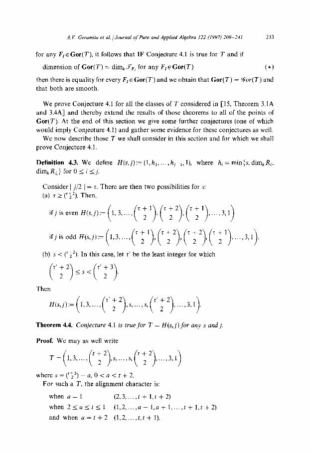
Definition 4.3. We define H(s,j):= (l,hl, . ,hj_l, l), where hi = min{s, dimk Ri, dim,Rj,l forO<i<j.

Consider Lj/2 J = z. There are then two possibilities for s: (a) s 2 (*:‘). Then,

ifjisevenH(s,j):=(l,i ,..., (‘:‘).(‘:‘).(‘i’) ,..., 3,l)

ifjisoddH(s,j):=(1,3 ,..., (‘:‘),(‘:2),(~~2),(‘:‘) ,..., 3,l).

(b) s < (‘12”). In this case, let z’ be the least integer for which

(“;“)Q<(‘:‘).

Then

H(s.j):=(1,3 ,..., (‘l’),s ,..., .s,(T’12) ,..., 3,1).

Theorem 4.4. Conjecture 4.1 is true for T = H(s, j) for any s and j.

Proof. We may as well write

.=(1,3 ,..., (‘;‘),s ,..., s,(“;‘) ,..., 3,1)

where s = (‘:“) - a, 0 < a 5 t + 2.

For such a T, the alignment character is:

when a = 1 (2,3, . . ) t + 1, t + 2)

when 21a1t~l (1,2 ,..., a-l,a+l,..., t+l,t+2)

and when a = t + 2 (1,2, . . . , t, t + 1).

234 A. V. Geramita et al. /Journal of Pure and Applied Algebra 122 (1997) 209-241

Clearly we must have j 2 2t, but

(a) if j = 2t then s = (’ :‘) and

H(s,j) = 1 3 ... (‘:‘) (tfi2) (‘:I) ... 3 1;

while

(/I) ifj = 2t + 1 then we must also have s = C’z2), but now

H(s,j) = 1 3 .” (“i’) (‘:‘) (‘:‘) (‘:I) ... 3 1.

In both cases, a = t + 2. We first deal with these two special cases. Case a: In this case it is easy to see that if I E [T] then there is only one possible set

of degrees in a minimal generating set for I, namely 2t + 3 generators of degree t + 1. Thus, (in the notation of Theorem 2.17 and Remark 2.18) we get that all of the first syzygies of I (there must be 2t + 3 of them) have degree t + 2.

Hence, for any I E [T] the minimal free resolution of l2 must be:

0 + p’+w~+3w( _(2t + 4)) + p+3)‘p1(_(2t + 3))

-+ R(2’+3)(2t+4)/2( -(2t + 2)) + 12 -+ 0.

Since j = 2t we obtain

dimk(Z2)2, = 0 and so dimk(R/12),, = dim, Rtt = .

It follows that

in this case. Case 8: Now we have j = 2t + 1 and s = (‘:‘) and (in the notation of Theo-

rem 2.17) b = 2t + 3. Any ZE[T] with the maximal number of generators has t + 2 = a generators of degree t + 1 and t + 1 generators of degree t + 2.

We write down the data of degrees and syzygies in the following tableau (see Section 3 for the notation):

o-times (t + 1 )-times

- w

t+ l......t+ 1 t+2......t+2 (4i)

t+3......t+3 t+2......t+2

- v (Pi)

o-times (f + l)-times

\2 . . . . . . V

2, O......O * Cri)

a~times (t + 1).times

A. V. Geramiia et al. /Journal of Pure and Applied Algebra 122 (1997) 209-241 235

Thus, any ideal I E [T] will have

a=t+2 generators of degree t + 1;

(t + 1) - 2v(v 2 0) generators of degree t + 2.

It follows that for any ideal ZE[T], the resolution of I* is:

0 + F, + F1 -+ F, + I2 + 0,

where

F. = R’(=+ ‘I’*( -(2t + 2)) @ R”@+’ -‘“‘(-(2t + 3))

@ R(‘+ 1 - 2V)(l + 2 -2V)/2 t-p + 4));

F1 = Ra(t + 1 - 2v) (-(2t + 3))@R”+‘-2”‘(-(2t +4))@R’(‘+1-2”)-1(-(2, + 5));

F2 = R”- 2V)(t + 1 - *I’)/2 (-2t + 4))@R”“+‘-2”(-(2t + 5))

@ Ra(a- I)/* (-(2t + 6)).

Thus dim,(Z2)2,+1 = 0 and so in this case we have,

dimk.9~,=dim,R2,+I - 1 = - 1

Aside: If we consider T = (1,3,6,6,3,1) (which fits into the case just considered for t = 2) we find that 6(T) = 5 and A(T) = 7. So, there are two possible degree sequences for minimal generating sets of ideals I E [T], i.e. v can be either 0 or 1 for this T. Thus the resolutions of Z* for Z E [T] can be different. But, a quick look at the resolutions above show that H(R/Z*, -) is independent of Z E [T], i.e. independent of v. We shall return to this comment later.

We now move to the general case,

j 2 2t + 2, t+3

T=H(s,j), s= 2 ( 1

-a, O<aIt+2.

We may apply the procedure of Theorem 2.17 (see also Remark 2.18) to produce an ideal Z E [T] with the maximum possible number of generators. For such an ideal we have the following data (see also Section 3 for notation):

a-times (t-a+*)-times

M - t+l......t+l t+2......t+2

(4i)

t+n......t+n t+n+l......t+n+1 M Y

(t-a + 2)-times (a - 1 )-times

236 A. V. Geramita et al. /Journal of Pure and Applied Algebra 122 (1997) 209-241

n-times (t -a + 2).times

I- *

\I

t+n+2......t+n+2 ;+n+l . . . . . .

t+3......t+3 t+2......t+2 w M

(t-a + 2).times (a 1).times

a-times (t--a+2)-times

h c \

n+l......n+l

(Pi)

3 __12.. . . .3 -n 1 __n . . . . . . 1 --y1 (ri)

v v (2 pa + 2)-times (a- 1).times

We observed that the generator degree sequence (qj) and syzygy degree sequence (pi) of any ideal Z’E [T] is obtained from that above by eliminating pairs of generator degrees (and syzygy degrees) corresponding to pairs of {a, -cx> among the Y;S.

Thus, any other ideal I E [T] will have:

a generators of degree t + 1;

(t - a + 2) - v generators of degree t + 2;

(a - 1) - v generators of degree t + n + 1;

and, if n # 3; t - a + 2 generators of degree t + n;

and if n = 3; (t - a - 2) - 2~ generators of degree t + n;

where v and v are 20. As in the special cases above, the idea is to use Theorem 3.2 to calculate dim, Ii for

I E [T] and to show that this dimension does not depend on v and q and only depends on t, a and n, i.e. only on T.

We will carry through the details in the case j = 2t + n, n > 3 and only report on the conclusions for the cases n = 2, 3. The ideas are identical in those cases as well.

So, let j = 2t + n, n > 3. Then, from Theorem 3.2 we have, for I E [T],

0 + (F2)j + CFl)j + CFO)j + (I’)j + O,

where

(J’o)j = R a(n'1)'2(-(2t + 2))jo Ra(*-a'2-V)(-(2t + 3))j

@ R(‘-a+2-v)(t-n+3-v)/2(_(2t + 4))j;

Note. F,, may have other free summands R( - m), but the others all have m > j and so R( -m)j = Rj_, = (0). The same comment applies to F1 and F2.

(F,)j=R”‘“-‘-“‘(_(2r + 3))j~Ra(r-~+2)+(~-1-v)(~-a+2-v)(_(2t +4))j

@ R”_ a+2)2-(f~o+2N_(2t + q)j

A. V. Geramita et al. /Journal of Pure and Applied Algebra 122 (1997) 209-241 237

and

(jTz)j = R@- 1 - “)@----vf/2(_(~t + 4f)j @ R(‘-“+2)(a-1 -“( _(2t + j)jj

@ R”_ a+2)(f-Q+1)/2(_(2t + fj))j_

We can see from these formulae that we must consider, separately, the cases when

n = 4, 5, or vz L 6. We do that now.

Case n = 4: So, we have j = 2t + 4. Then

a(a + 1) dim,(I’)j = 2 - dim, R2 + a(t - a + 2 - v)dim, RI

+

(t - a + 2 - v)(t - a + 3 - ‘) -

u(u _ 1 _ v)dim R

2 k 1

- a(t - a + 2) - (a - 1 - v)(t - a + 2 - v)

+ (a - 1 - v)(a - 2 - v)

2

A simple calculation shows that this last is equal to

6 + it2 + $t + 3~x2

which is independent of v, as we wanted to show.

It follows that

dim,&, + 1 = H(R/I’, 2t + 4) = (?t;6)- (6+;t’+;l+3a)

and so

dim, FF, = St2 + yt + 8 - 3~.

Case n = 5: We set j = 2t + 5, then

a(a + 1) . dimk(12), = 2 ~ dlmk R3 + a(t - a + 2 - v)dim, R2

+ (t - a + 2 - v>(t - a + 3 - V)dim

k 1

R _ a(a _ 1 -

2 v) dim, R2

- (dimk R,)[a(t - a + 2) + (a - 1 - v)(t - a + 2 - v)]

+ (a - 1 - $(a - 2 - v) dim R

2 k I

- (t - a + 2)2 + (t - a + 2)~ + (t - a + 2)(a - 1 - v).

A simple calculation shows that this last is equal to

12 + St2 i- yt + 3a

238 A. K Geramita et al. /Journal of Pure and Applied Algebra 122 (1997) 209-241

which is independent of v, as we wanted to show. It follows that

dim,FF,+ 1 =H(R/12,2t+5)=(2t~7)-(12+~t2+~t+3a)

and so

Note that this is the same result we obtained forj = 2t + 4. Case y1 2 6: Nowj = 2t + II where n 2 6. Then precisely the same sort of computa-

tion as above gives that

dim,FF,=st2+yt+8-3a

which is independent of both v and n. Aside: So, we see that the calculation of dimkFFr depends only on t and a when

j = 2t + n and n 2 4. This is not same value we will find when n = 2 and n = 3. Case n = 3: Since j = 2t + 3, the free resolution of (Z”)j is now given by

(F,)j = R“(“+ l)j2 (-(2t + 3))jo R”‘(‘-U’2~Y’(-2t + 3))j

while

(,J7,)j = @-l-“) (-(2t + 3))j and (F2)j = (0).

(Notice that y does not even appear in this part of the resolution for I’.)

So,

dim,(12)j = (dim, RI) + a(t - a + 2 - v) - a(a - 1 - v)

Thus

and so

dimkFF, = 2t2 + (9 - a)t + (9 + fa2 - %a).

Case n = 2: Now we have j = 2t + 2. Omitting the details, we get

dimk .FF, = 2t2 + 7t + (5 - ia2 - fa).

This completes the proof of the theorem. 0

Corollary 4.5. Let T = H(s,j) for s = (“2”) - a where 0 -L a 5 t + 2. Zf j = 2t + n

where n 2 4, then %or(T) = Set,- l(Vj(P’)).

A. V. Geramita et al. /Journal of Pure and Applied h&e&a 122 (1997j 209-241 239

Proof. We first observe that the dimension of the variety Set,_ i(vj(P’)) = 3s - 1. This is so because the only deficient secant varieties of Veronese Surfaces occur either when j = 2 or when j = 4 and s - 1 = 4 (Cl], see [lo] for a discussion) and these are cases not covered by the hypothesis.

One then checks that

3.s-1=“t2+15t+8-3a. 2 2

This is precisely the dimension we found for J KF, for every I E [IT] and that is enough to finish the proof. 0

Remark 4.6. (a) This corollary should be compared with Theorem 3.1A and Theorem 3.4A of [15].

(b) It would be interesting to know if, for the T of the corollary,

%or( I T) = %or(T) (see [15, Example 5.81). (c) The following example is interesting and points out some things that we still do

notknow.Lets=7,i.e.s=10-3sothatt=2anda=3.Choosej=9=2.2+5 so that Corollary 4.5 applies to T = (1, 3, 6, 7, 7, 7, 7, 6, 3, 1).

There are two interesting catalecticant matrices associated to this example; the first, A (a 10 x 28 matrix), describes the third partials of a general form of degree 9 and the second, B (a 15 x 21 matrix), describes the fourth partials of a general form of degree 9.

We know that Yor( I T) is described by the ideal I = Z,(A) + Z,(B) and we have shown that the primary decomposition of I = pnq, where @ is the prime ideal which describes the variety Sec,(v,(P*)) & P(S,) (S = k[y,, y,, y2]) and q is primary for the irrelevant ideal in the homogeneous coordinate ring of P(S,).

It would be interesting to know if I is a saturated ideal (we believe that it is) and show that q does not appear in the primary decomposition of I.

It would also be interesting to know if Z,(A) g Z,(B) (a reasonable assumption since rkB I 7 * rkA I 7). But, this last problem is about equations and not just about the underlying reduced variety and so the statement about ranks remains only an “indication”.

This is just one of a family of such questions suggested by Corollary 4.5. In view of the corollary, the only T = H(s,j) for which we have not yet proved that

%x-(T) is smooth and equal to Gor(T) are those T for which s = (‘>“) - a, where O<a1t+2andj=2t+n,whereO1n13.

Remark 4.7. We have seen that ifj = 2t or 2t + 1 then the only s we need consider is s = (“,“), corresponding to a = t + 2. But, in both of those cases it is easy to see that Gor( I T) = 9or( < T) = P(Sj) which is of dimension

(i+22)=(2t12) (ifj=2t) or (,‘l’) (ifj=2t+l).

So, the only cases still left to consider arise when eitherj = 2t + 2 orj = 2t + 3.

240 A. V. Geramita et al. lJourna1 of Pure and Applied Algebra 122 (1997) 209-241

Example 4.8. Consider T = (1, 3, 5, 3, 1) (cf. Example 1.2). In this case s = 6 - 1 = 5 andsot=l,a=landj=4=2t+2.

From Theorem 4.4 we obtain that for Ze [T], dim, Yp, = 13.

We can conclude, then, that 9?or(T) = Sec4(v4(P2)). Note that this is one of the deficient secant varieties to a Veronese Surface. In fact, a simple check (using Theorem 4.4) shows that all the inequalities of Example 1.3(3) are equalities and we obtain that Gor(T) = gor(T) for all the T of that example.

We can say something more in the casei = 2t + 3.

Proposition 4.9. Let s = (‘:“) - a, where 0 < a I t + 2 and let j = 2t + 3.

Zfu = 1, 2, t + 1 or t + 2 then Gor(T) = Yor(T) and so Gor(T) is smooth in these

cases.

Proof. In these cases Iarrobino and Kanev have found the dimension of Gor( T) [ 15, Theorem 3.4B] and it is the same as the dimension of the tangent space to Yor(T) at every one of its closed points (from Theorem 4.4). In view of Remark 4.2 that is enough to prove the proposition. 0

Remark 4.10. It would be very interesting to know if Gor(T) = Yor(T) for every T = H(s,j).

If T = H(s,j) it is not hard to show (although the calculations are tedious) that whenever I, J E [T], then 1’ and J* have the same Hilbert function. It is reasonable, therefore, to conjecture:

Conjecture 4.11. If I and .Z are homogeneous ideals in R = k [x0, . . , x3] of codimen- sion 3 for which R/Z and R/J are Gorenstein with the same Hilbert function then R/Z*

and R/J* have the same Hilbert function.

Having made that conjecture, it makes sense to conjecture the analogous result for codimension two Cohen Macaulay ideals. More precisely,

Conjecture 4.12. Let Z and J be ideals of points in ip*. If R/Z and R/J have the same Hilbert function then the same is true for R/Z* and R/J*.

Remark 4.13. (a) A weaker conjecture then Conjecture 4.12 in which we only assume that R/Z and R/J are arithmetically Cohen-Macaulay and of codimension 2 is false, as an example of Peterson shows (see [19]).

(b) A proposition of Iarrobino-Kanev [ 15, Theorem 3.6.11 gives some evidence for the truth of Conjecture 4.12. They prove the weaker result that Conjecture 4.12 is true if Z and J are both the ideals of a set of points in p2 with generic Hilbert function and

minimum number of generators possible for tht Hilbert function.

A. V. Geramita et al. /Journal of Pure and Applied Algebra 122 (1997) 209-241 241

Acknowledgements

It is our pleasure to thank Tony Iarrobino and Vasil Kanev for responding so

graciously to our many questions about their joint work. We also thank Susan Diesel

for sending us an advance copy of her paper.

References

[l] J. Alexander, A. Hirschowitz, Polynomial interpolation in several variables, J. Algebraic Geom.

4 (1995) 201-222.

[2] M. Boji, D. Laksov, Nonunimodality of graded Gorenstein Artin algebras, Proc. Amer. Math. Sot.

120 (1994) 108331092.

[3] D. Bernstein, A. Iarrobino, A nonunimodal graded Gorenstein Artin algebra in codimension five,

Comm. Alg. 20 (1992) 232332336. [4] D. Buchsbaum, D. Eisenbud, Algebra structures for finite free resolutions and some structure

theorems for ideals of codimension 3, Amer. J. Math. 99 (1977) 447-485.

[S] G. Campanella, Standard bases of perfect homogeneous polynomial ideals of height 2, J. Algebra 101

(1986) 47-60.

[6] C. Ciliberto, A.V. Geramita, F. Orecchia, Remarks on a Theorem of Hilbert-Burch, Boll. Un. Mat.

Ital. B (7) 2-B (1988) 463483. [7] E.D. Davis, A.V. Geramita, P. Maroscia, Perfect homogeneous ideals: Dubreil’s theorems revisited,

Bull. Sci. Math. (2) 108 (1984) 143-185.

[S] E. DeNegri, G. Valla, The h-vector of a Gorenstein codimension three domain, preprint.

[9] S.J. Diesel, Irreducibility and dimension theorems for families of height 3 Gorenstein algebras, Pacific

J. Math., to appear.

[lo] A.V. Geramita, Waring’s problem for forms: inverse systems of fat points, secant varieties and

Gorenstein Algebras, Queen’s Papers in Pure and Applied Math., No. 105 (1996) The Curves Seminar,

Vol. x.

[l l] A.V. Geramita, P. Maroscia, L. Roberts, The Hilbert function of a reduced K-algebra, J. London

Math. Sot. (2) 28 (1983) 443452.

[12] A.V. Geramita, J.C. Migliore, Hyperplane sections of a smooth curve in P3, Comm. Algebra 17 (1989)

312993164.

[ 133 A.V. Geramita, J.C. Migliore, Reduced Gorenstein codimension three subschemes of projective space,

Proc. Amer. Math. Sot., to appear.

[14] T. Harima, Some examples of unimodal Gorenstein sequences, preprint.

[15] A. Iarrobino, V. Kanev, The length of a homogeneous form, determinantal loci of catalecticants and

Gorenstein algebras, preprint.

[ 161 A. Kustin, B. Ulrich, A family of complexes associated to an almost alternating map, with applications

to residual intersections, AMS Memoirs, Vol. 95, No. 461 (1992) Providence, RI.

[17] J.C. Migliore, An introduction to deficiency modules and liaison theory for subschemes of projective

space, Lecture Note Series, No. 24, Research Institute of Mathematics - Global Analysis Research

Center, Seoul National University, Seoul, Korea.

[lS] C. Peskine, L. Szpiro, Liaison des varietes algebriques, I, Invent. Math. 26 (1974) 271-302.

[19] C. Peterson, Powers of ideals and growth of the deficiency module, Queen’s Papers in Pure and

Applied Mathematics, No. 95, The Curves Seminar at Queen’s: vol. IX (1993).

[20] L. Roberts, M. Roitman, On Hilbert functions of reduced and of integral algebras, J. Pure Appl.

Algebra 56 (1989) 855104.

[Zl] P. Schenzel, A note on Dubriel’s theorems and the number of generators of perfect ideals of

codimension 2, CR. Math. Rep. Acad. Sci. Canada VI (1) (1984) 1 l-14.

[22] R. Stanley, Hilbert functions of graded algebras, Adv. Math. 28 (1978) 57783.