Road following using vanishing points

COMPUTER VISION, GRAPmCS, AND IMAGE PROCESSING 39, 116-130 (1987)

NOTE

Road Following Using Vanishing Points

SHIH-PING LIOU AND RAMESH C. JAIN

Computer Vision Research Laboratory and Robot Systems Dioision, Department of Electrical Engineering and Computer Science,

The University of Michigan, Ann Arbor, Michigan 48109

Received January 15, 1986; accepted July 30, 1986

The location of a vanishing point determined by boundaries of a road indicates the direction of the road. The detection of reliable road boundaries is a nontrivial task in most scenes, however. We propose an algorithm that uses hypothesized vanishing points to extract the road boundaries. Based on the direction and strength of edges in an area for a hypothesized vanishing point, a performance measure is computed. This performance measure reflects confidence in the hypothesis that the given vanishing point is the correct vanishing point for the road. The vanishing point for the given image, and the corresponding road boundaries is selected by searching for the maxima of the performance measures. The efficacy of our approach is demonstrated using several real-world road images. © 1987 Academic Press, Inc.

1. INTRODUCTION

Autonomous mobility is attracting growing attention from computer vision and artificial intelligence researchers [WMS85, TYA85, Mor81, Mor83, Ni169, GSC79, Tsu84, YIT83, IMB84, TMM85, DaK85, WST85]. The roadway boundary 1 location problem has become an important problem in visual navigation tasks. In a con- strained environment this problem is easy, but for real roads in different real world situations, this has been a formidable task. The difficulties are due to variable contrast in images, a wide range of intensity values of the road surfaces, and presence of intersection and other confusing artifacts for the algorithm. To make this problem harder, the processing speed of the algorithm should be satisfactory for driving a vehicle above a specified minimum speed.

One of the earliest autonomous navigation systems was the Stanford Cart and Robot Rover described in [Mor81, Mot83]. In that system, there was no need to detect roadway boundaries and real time operation was not considered. A visual navigation system is being built at the University of Maryland to enable a vehicle to follow roads. Their approach comprises a boot-strap phase [WMS85] and a feed- forward phase [DaK85]. They use the conventional image processing techniques such as filtering, sobel edge detector, histogram analysis, segmenting, shrinking and expanding, and Hough transform in the boot-strap phase. The initial finding of the road edges needed 120 CPU sec on a VAX 780. In the feed-forward phase, they used the pivot point, the endpoint of the line in the previous window, to constrain the search space as well as to eliminate the use of line fitting techniques. Like the idea presented in [WST85], they selected windows instead of processing the entire image. In a sequence of images, this idea of selecting a window for finding road edges is very important for reduction in computational requirement.

A mobile robot system designed for indoor scenes is described in [TYA85]. The knowledge of the environment, the abundance of vertical edges in the scene, and the

1The terms roadway boundary and road edges will be used interchangeably in this paper.

116

0734-189X/87 $3.00 Copyright © 1987 by Academic Press, Inc. All rights of reproduction in any form reserved.

VANISHING POINTS 117

flatness of the floor, were used as constraints for the dynamic scene analysis. This robot moved at a speed of 0.3 m/sec in a building containing moving objects. This system demonstrated the application of domain knowledge in finding navigable areas in the environment.

Another system FIDO, based on the Stanford Cart and Robot Rover and improved by using parallel hardware, reduced the run time from 15 minutes to less than a minute per step [TMM85]. Inigo et al. [IMB84] proposed a set of algorithms, implementable in real time, for roadway boundary location and obstacle detection. However, since only left road edge was detected in their algorithms, this method would face difficulties not only in the estimation of roadway boundaries but in the determination of moving direction also.

A complete vision system for an autonomous land vehicle was presented by Wallace et al. [WST85]. Not only low-level motor drivers but top-level control loop and user interface were both covered in their system. However, though several mechanisms were tried to extract lines and edges, none of them worked all the time. The following assumptions were made by the authors:

(a) The road is straight; thus, predictions can be made by linearly extending the road edges.

(b) The camera's calibration, roadway, and orientation with respect to the road are known.

(c) The ground is locally level and all candidate edges arise from ground feature.

This system, essentially a feedback system, used the model edges to generate two small subimage rectangles in which to search for the left and right roadway boundaries. After obtaining all edges in subimage rectangles, the system selected a pair of extracted edges as the roadway boundaries. However, without further information about the direction of the roadway boundaries, the system will prob- ably lead to a poor performance especially in handling bad-contrast pictures.

By simplifying the problem and using some ideas of the Vanishing Point (VP) analysis, we propose an algorithm called Vanishing-Point Road-Edge Detector to extract the images of the roadway boundaries. To avoid using any data-driven line fitting or approximation technique in the algorithm, a set of convergent lines is used to speed up the process. Essentially, for a hypothesized vanishing point we collect evidence supporting it from the image. The supporting evidence comes from the strength and direction of edge points and length of line segments. We define functions to measure the support of each evidence and combine them in the performance measure that gives confidence in the VP. The VP having highest confidence is selected and the corresponding convergent lines are considered as the images of the roadway boundaries.

2. SCENE AND IMAGE

Our aim is to recover 3-D information about the scene from its images. In this section, road model will be described first. Following that, review of the research on vanishing point analysis is given and the analysis on the roadway boundary location problem will be explored at the end.

118 LIOU AND JAIN

2.1. Road Model

We assume that road segments can be approximated by straight lines. Thus segments of road boundaries can be modeled as

R = XcosO + YsinO, (1)

where (X, Y) is any point on the line, R is the distance from the origin to the line and 0 is the angle between the X axis and the vector from the origin normal to the line.

Note that for controlling the vehicle which is moving very slowly with respect to the frame processing time, the boundaries near the vehicle are more important. In most cases, the assumption of linear boundaries is satisfied reasonably well for the boundaries near the vehicle. Usually, on turning roads the vehicle is driven slowly; some other knowledge source might be required to achieve faster speed.

2.2. Vanishing Point Analysis

The perspective projection of any set of parallel lines which are not parallel to the image plane converges to a vanishing point [FoD82]. The location of the vanishing point depends only on the orientation of the lines. Thus, by considering the road edges as the lines mentioned above, the location of vanishing points allows us to constrain their possible positions and other known structures in an image.

Determination of the vanishing points has attracted the attention of many researchers [Bar82, TYA85, MaA84, Ken79, Bad74]. Kender [Ken79] presented two approaches for determining vanishing points; one of them maps line segments with a common vanishing point into circles that pass through the origin, and the other transforms lines with the same vanishing point into a common line in the inverted space. Badler [Bad74] discussed a method based only on cross products of line segments to extract vanishing points. A computationally inexpensive algorithm which is similar to [Bad74] was described by Magee and Aggarwal [MaA84] for the determination of vanishing points, once line segments in an image had been determined. The relationship between vanishing points, vanishing lines, and the gradient space was explored by Shafer, Kanade, and Kender [SKK82]. Tsuji, Yagi, and Asada [TYA84] used the invariance property of vanishing points to make the estimation of the rotational component.

Most researchers proposed methods to either determine vanishing points from the given line segments or to search line segments which converge to the given vanishing point. In real road scenes, determining reliable line segments is difficult, making the problem of locating vanishing points tedious. However, since a vanishing point is associated with a set of parallel lines, and, furthermore, the vehicle action, which needs only a relevant information, is purposive, the hypothesize-and-test technique can be applied in cooperation with the vanishing analysis and thus forms an efficient parallel algorithm to detect the roadway boundaries as well as vanishing point simultaneously.

2.3. Problem Requirements and Analysis

To find road edges, one approach is to detect all edge points in a frame and then interpret these points. Conventional edge detectors do not provide accurate solu-

V A N I S H I N G P O I N T S 119

tions to the roadway boundary location problem without some kind of line fitting operation after edge detection. Since most techniques for line fitting are slow, the task of roadway boundary location in real time is usually difficult.

To simplify the problem, low curvature roadway boundaries and locally level ground driving are assumed. In that case, the tangent direction to the roadway edges, at any time instant, can provide sufficient information for vehicle guidance and these tangent lines will meet at a vanishing point. Let us define the road vanishing point at time t, denoted by RVP/, to be a vanishing point at which the tangents to the images of the current roadway boundaries at time t will converge. Moreover, since the road curvature changes smoothly, RVP will only move slightly and, therefore, the system will be able to keep track of the RVPs even on a bending road.

Now, since the location of the vanishing point does not change much between two contiguous frames, we can assume that its location in the current frame will be same as in the previous frame. This fact allows combining road edge detection and vanishing point determination in one step. By assuming a search window around the previous-frame position of the vanishing point, we may find the best vanishing point in the current frame using a measure based on edges and their characteristics in the frame.

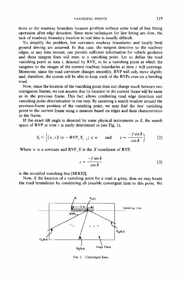
If the exact tilt angle is detected by some physical instruments as 8, the search space of RVP at time t is easily determined as (see Fig. 1),

- f sin ~ ) S t= ( x , z ) l [ x - R V P X~ 11 < w and z (2)

- cos

Where w is a constant and RVP_X is the X coordinate of RVP,

- f sin z (3)

cos

is the so-called vanishing line [SKK82]. Now, if the location of a vanishing point for a road is given, then we may locate

the road boundaries by considering all possible convergent lines to this point. We

St Vk(t )

. . . . . . . . . . . . . . . . . . . . . ~ . . . . . . . . . . . . . . . . . . . Vanishing

_~R~ ~, . . ~ ~ce, (k,t) \

Coi(k,t) Image Plane

FIG. 1. Convergentlines.

Line

120 LIOU AND JAIN

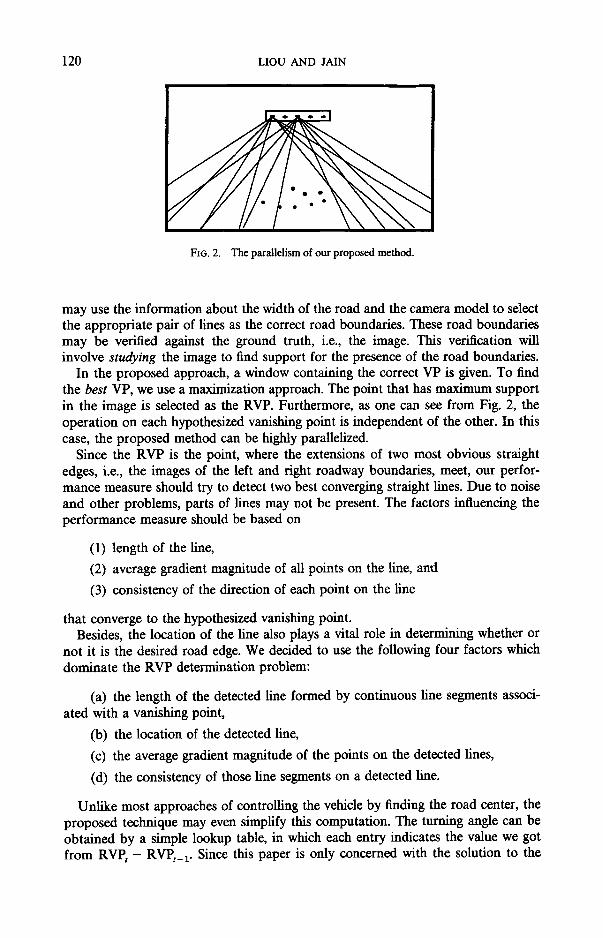
FIG. 2. The parallelism of our proposed method.

may use the information about the width of the road and the camera model to select the appropriate pair of lines as the correct road boundaries. These road boundaries may be verified against the ground truth, i.e., the image. This verification will involve studying the image to find support for the presence of the road boundaries.

In the proposed approach, a window containing the correct VP is given. To find the best VP, we use a maximization approach. The point that has maximum support in the image is selected as the RVP. Furthermore, as one can see from Fig. 2, the operation on each hypothesized vanishing point is independent of the other. In this case, the proposed method can be highly parallelized.

Since the RVP is the point, where the extensions of two most obvious straight edges, i.e., the images of the left and right roadway boundaries, meet, our performance measure should try to detect two best converging straight lines. Due to noise and other problems, parts of fines may not be present. The factors influencing the performance measure should be based on

(1) length of the line,

(2) average gradient magnitude of all points on the line, and

(3) consistency of the direction of each point on the line

that converge to the hypothesized vanishing point. Besides, the location of the hne also plays a vital role in determining whether or

not it is the desired road edge. We decided to use the following four factors which dominate the RVP determination problem:

(a) the length of the detected line formed by continuous line segments associated with a vanishing point,

(b) the location of the detected line,

(c) the average gradient magnitude of the points on the detected lines,

(d) the consistency of those line segments on a detected line.

Unlike most approaches of controlling the vehicle by finding the road center, the proposed technique may even simplify this computation. The turning angle can be obtained by a simple lookup table, in which each entry indicates the value we got from RVP t - RVP t_ t- Since this paper is only concerned with the solution to the


roadway boundary location problem, we will not discuss the control problem in more detail.

3. PROPOSED VANISHING-POINT ROAD-EDGE DETECTOR

The proposed algorithm can be implemented on multiprocessors such that each processor essentially works using a hypothesized vanishing point.

According to Eq. (2) and within a present tolerance a, the coordinates of all possible vanishing points can be calculated as:

x k = RVP_Xt_ 1 - w + ka,

- f sin 8 2w Zk COS8 ' V k = 0 , - - a

(4)

Let us denote the kth vanishing point at time t as Vk(t ) and define the convergent line with an angle s, represented by Cs(k, t), to be a fine segment that crosses the image plane and its extension passes the vanishing point V k (t).

We divide all convergent fines into two categories, the images of all left- and fight-roadway boundaries. Furthermore, since the location of the convergent fines from any given hypothesized vanishing point remains the same at every time instant, the coordinates of the points which are located on these different convergent fines can be calculated before the vehicle has moved at all. By storing the precomputed results, we will therefore save our efforts in determining the road vanishing point.

Let us define pixel element (d, m), , j to be a pair of data derived from the estimate of the gradient magnitude m and edge orientation d at pixel location (i, j ) and let L, be the adjustment ratio which is a preset tolerance used for the safety purpose.

According to Eq. (4), for the VPRE detector algorithm, (2w/a) + 1 processors are used to achieve the parallel performance. This algorithm is stated as

Algorithm. Vanishing-Point Road-Edge Detector.

Notation: conofound indicates the angle of the convergent line found as the most promising road edge in each category and value found is the performance measure of this convergent fine. m~ is a general notation for the performance measure of a convergent fine with angle i

1. Produce the corresponding pixel elements at each precomputed location. 2. For each processor k at time t do.

Begin. 3. For each convergent line Cs(k, t) as illustrated in Fig. 1

Compute the performance measure. 4. For each category do.

Begin. 5. Find the convergent line which has the maximum performance

measure among all fines (suppose this line is with angle i and its corresponding measure is m~).

6. Set conv._found to i, value_found to m,.

1 2 2 LIOU AND JAIN

. While there exists a convergent line with angle j which has performance m e a s u r e mj such that

[mcono found-- mj] < t r* mconv_found

Set cono..found to j , value_found to mj.

(5)

8. The convergent line with angle cono__found is the image of the hypothesized roadway boundary in this category.

End. 9. Set the performance measure of Vk(t ) tO be the minimum of the perfor-

mance measures in these two categories. End.

10. Select the vanishing point which has the maximum performance measure as the RVP and its corresponding convergent line, in each category, which has the maximum performance measure as the road edge.

End of Algorithm

4. IMPLEMENTATION DETAILS

In our studies we decide to use a simple edge detector to investigate the efficacy of our approach. A better edge detector will improve the performance. Due to good computational efficiency and reasonable performance, the Sobel edge finder is used to compute the direction and magnitude of the gradient at a point i, j where the intensity is f,., j . Thus we define the partial derivative estimates

S~(i, j ) =fi+l, j+l + 2f/+s,j + L + I , j - I - f i - l , j + x - 2L-x,j-L-I,j-1, (6)

Sy(i, j ) = f/-x,j+x + 2f/,j+l + fi+l,j+l - f i - l , j -1 - 2f,,j-x - fi+l,j-1. (7)

The Sx and Sy partial derivative estimates are then combined to form an estimate of the gradient magnitude m, and direction d by

m = ISxl + ISyl,

_lFSyl (8) . - - , a n

The magnitude and direction maps are both quantized to eight bits to form the pixd dement (d, m)i ' j.

Now, let us define the edgepoint to be a point whose pixel element is (d, m) such that for a convergent line C~(k, t)

]d - sl <- to and m > ts, (9)

where t s and t s are both threshold values. Note that we are interested only in those edge points that are on convergent lines.

Other points will not enter into considerations irrespective of their strength. Next,


we form line segments out of these edge points as follows. Let t d represent the allowed maximum length of continuous non-edge points, and L 1 mean the minimum length of continuous edge points. We define the line segment to be a line with the number of continuous edge points greater than t I. Two sets of continuous edge points separated by a series of non-edge points whose length is less than l d are considered a line segment, if the total length is greater than t 1.

To avoid the digitization problem when searching for a vanishing point, we, in real implementation, give some tolerance in the Z direction on both sides with fixed tilt angle.

4.1. Performance Measure

From all points along C,(k, t) for some s and Vk(t), we extract all the qualified line segments. Finally, a decision is made over all convergent lines by a measure of the system's confidence in how well the lines are formed.

For finding good lines, we used the following performance measure functions with normalized value in a range from 0 to 1. The reason of normalization is that we like to have the final performance measure in that range after we combined all the dominating factors.

(A) The length of the detected line formed by continuous line segments associated with a vanishing point

Gk Leng(x, k) = - - (10)

DMax

where Dxk = total length of all line segments detected along the convergent line Cx(k, t), and DMa x is the maximum length value for all possibilities.

(B) The location of the detected line

1 Close(x, k) 1 + q~' (11)

where qz is the Z coordinate of the points which is nearest to the X axis and also located on the detected line.

(C) The average gradient magnitude of the points on the detected lines

E mi,j Mag(x, k) (i,j)~G

255N(Ex) , (12)

where m i, j means the gradient magnitude component of the pixel element (d, m)i, j and N(Ex) means the amount of all edge points found along the convergent line G (k, t).

124 LIOU AND JAIN

(D) The consistency of those line segments on a detected line whose direction is Ox,

Cons(x, k) y , ~r - 21d , j - Oxl / N = --' (Ex), (13) (i,j)~Ex /

where di, j means the direction component of the pixel element (d, m)i,j. The performance measure ~(x, k) is then defined as

h (x , k) = w , . Leng(x, k) + w 2 • Close(x, k) + w 3

• Mag(x, k) + w 4 • Cons(x, k) , (14)

where w,., i = 1 . . . . . 4 are the preset weights and the value of x and k are associated with a convergent line Cx(k , t) at time instant t.

In our experiments, we empirically chose weights 0.8, 0.03, 0.06, and 0.11 for wl, w 2, w 3, and w 4, respectively. To be more robust, these weights should be changed as the vehicle moves to different places. We can adjust the weights to emphasize different factors.

Now, by using ~, + and ~ - to represent the measure in these two categories separately, the purpose is to find x and y such that

X + ( x , k ) = M A X { X + ( i , k ) } , V i ~ A , (15)

h - ( y , k ) = M A X { X - ( i , k ) } , V i ~ B ,

TABLE I Summary of Experiment A

Picture sequence No. of frames/data sampled Search window set RVP found

1 64/3 (105,205), (155,210) (135,210) (107,205), (157,210) (137,210) (105,205), (155,210) (120,205)

2 64/3 (85,232), (135,237) (115,237) (70,205), (120,210) (90,210) (72,229), (122,234) (117,234)

3 64/4 (95,205), (145,210) (130,205) (95,205), (145,210) (120,210) (95,205), (145,210) (120,210) (95,205), (145,210) (125,205)

4 64/3 (113,205), (163,210) (138,205) (113,205), (163,210) (143,205) (113,205), (163,210) (133,205)

5 400/4 (129,205), (179,215) (144,205) (119,205), (169,210) (144,205) (119,205), (169,210) (144,205) (144,205), (194,210) (159,205)

6 400/4 (46,205), (96,215) (66,205) (41,205), (91,210) (66,210) (41,205), (91,210) (86,205) (61,205), (111,210) (101,205)


where A and B indicate the category of convergent lines as the images of the left and right road edges separately.

Next let us define X as

x ( k ) = MIN{X+(x, k) , A - ( y , k ) ) . (16)

By combining the information from RVP t_ 1 as well as X, the process will make the final decision on the RVP t position. The decision is made by selecting the vanishing point Vt(t ) such that

X( I ) = M A X ( x ( k ) } , VV~( t ) e S t . (17)

4.2. Experimental Results

The performance of the Vanishing-Point Road-Edge Detector was tested using several real-world road image sequences on VAX 11-780 with the required processing time for a single convergent line ~ sec. Theoretically speaking, this time approxi- mates the time required to find road edges using parallel computation. The results of part of these sequences are briefly illustrated in Table 1. The first column in this

TABLE 2 Summary of Experiment B

Frame No. RVP detected

1 (105,189) 2 (110,184) 3 (110,184) 4 (120,179) 5 (120,179) 6 (120,179) 7 (120,179) 8 (120,174) 9 (120,174)

10 (120,174) 11 (120,174) 12 (120,174) 13 (120,174) 14 (120,174) 15 (120,174) 16 (120,174) 17 (120,174) 18 (120,174) 19 (120,174) 20 (115,174) 21 (120,174) 22 (145,169) 23 (120,169)

126 LIOU AND JAIN

FIG. 3. The first frame in picture sequence 1. (a) original picture, b) direction map, c) magnitude map, d) output picture.

table shows the number of the picture sequence, while column two shows the number of recorded frames as well as the number of sampled pictures. Following that, the search window St, as given in Eq. (2), is described in the next field by using the coordinates of the left-bottom and right-top points. The coordinates of the RVP found using the described approach are given in the last column. In addition, we also experiment with a longer sequence, where 23 continuous frames show a

FIr. 4. The first frame in picture sequence 2. a) original picture, b) direction map, c) magnitude map, d) output picture.


FIG. 5. The first frame in picture sequence 3. a) original picture, b) direction map, c) magnitude map, d) output picture.

left-turning road; during this part of sequence, the RVP does not change much. The result of detected RVP is shown in Table 2.

Figures 3-8 show the original pictures and the road edges with the vanishing points found by our approach. For the first four sequences short-interval frames were used, whereas for the remaining sequences we used long-interval frames. In each figure, (a) is the original picture, (b) and (c) are the direction and magnitude


128 LIOU AND JAIN

FIo. 7. The first frame in picture sequence 5. a) original picture, b) direction map, c) magnitude map, d) output picture.

maps derived from the Sobel edge detector, and the output picture with the lines showing the roadway boundaries and the box illustrating the search space is presented in (d). We found that the resulting edges are very good even for the poor contrast pictures (Figs. 3, 7, and 8). In addition, the results for the Sequences 5 and 6 show that it is not necessary to work with short-interval frames in a sequence. Thus the proposed method offers a robust method for detecting road edges for visual navigation tasks.



5. CONCLUSION

This paper presents an approach for locating the road edges. Since the direct application of the conventional image processing techniques does not result in reliable roadway boundary location, we utilized some general assumptions to simplify the analysis, and introduced the idea of vanishing point analysis to speed this approach. Our approach finds the best vanishing point for the images of the road edges using a criterion based on the quality of line segments detected in an image. This step combines the task of locating a vanishing point and finding the images of the road edges. In this respect this approach may be considered similar to approaches proposed for finding the focus of expansion by [Law84, JeJ84].

In our experiments we used Sobel operator for computing the pixel elements. The motivation for using this operator was the real-time requirements and our desire to see the performance of the approach with the modest quality edges. Our results suggest that a simple multiprocessor system may be able to detect roadway boundaries in real time even for complex scenes.

The search window for determining the VP in a frame of the sequence will be determined by the location of the VP in the previous frame. This fact allows automatic determination of the search window in each frame. Moreover, the location of the VP in the sequence will be determined by the curvature as well as slope of the road and more accurate weighting factors can also be obtained by several training samples. By determining these variations, information for steering the vehicle and for the formation of a model of the road may also be achieved with only a little additional computational cost. We plan to explore this using longer sequences of known roads.

[Bad741

[Bar82]

[Dak85]

[FoD82]

[GSC79]

[IMB84]

[JeJ84]

[Ken79]

[Law84]

[MaA84]

[Mor81] [Mor83] [Nil69] [SKK82]

REFERENCES

N. Badler, Three-dimensional motion from two-dimensional picture sequence, in Proceedings, IJCPR, Copenhagen, Denmark, August 13-15, 1974, pp. 157-161. S. T. Barnard, Methods for interpreting perspective images, in Proceedings, Image Under- standing Workshop, Stanford Univ., Palo Alto, Calif., 1982, pp. 193-203. L. S. Davis and T. R. Kushner, Road Boundary Detection for Autonomous Vehicle Navigation, CS-TR-1538, Center for Automation Research, Univ. of Maryland, July 1985. J. D. Foley, and A. Van Dam, Fundamentals of interactive computer graphics, Addison-Wes- ley, Reading, Mass., 1982. G. Giralt, R. Sobek, and A. Chatila, A multi-level planning and navigation system for a mobile robot, in Proceedings, 6th IJCAL Tokyo, 1979, pp. 335-337. R. M. Inigo, E. S. McVey, B. J. Berger, and M. J. Wirtz, Machine vision applied to vehicle guidance, IEEE Trans. Pattern Anal. Mach. Intelligence 6 (6), 1984, 820-826. C. Jerian and R. Jain, Determining motion parameters for scene with translation and rotation, IEEE Trans. PAMI, 6 (4), 1984, 523-530. J. Kender, Shape from texture: An aggregation transform that maps a class of textures into surface orientation, in Proceedings, IJCAI, Tokyo, Japan, August 1979, pp. 20-23. D. T. Lawton, Processing Dynamic Image Sequence from a Moving Sensor, Ph.D. dissertation (TR 84-05), Computer and Information Science Department, Univ. of Mass., Amherst, 1984. M. J. Magee and J. K. Aggarwal, Determining vanishing points from perspective images, Comput. Vision, Graphics, Image Process. 26, 1984, 256-267. H. P. Moravec, Robot Rover Visual Navigation, UMI Press, Ann Arbor, Mich. 1981. H. P. Moravec, The Stanford Cart and the CMU Rover, in Proc. IEEE 71, 1983, 872-884. N. G. Nillson, A mobile automation, in Proceedings, 1st IJCAL 1969, pp. 509-520. S. A. Sharer, T. Kanade, and J. R. Kender, Gradient space under orthography and perspective, in IEEE 1982 Workshop on Computer Vision: Representation and Control, Franklin Pierce College, Rindge, N.H., August 23-25, 1982, pp. 26-34.

130 LIOU AND JAIN

[TMM85]

[Tsu84]

[TYA851

[WMS85]

[WST851

[YIT83]

C. Thorpe, L. Matthies, and H. Moravec, Experiments and thoughts on visual navigation, in Proceedings 1985 IEEE Int. Conf. on Robotics and Automation, St. Louis, March 1985, pp. 830-835. S. Tsuji, Monitoring of a building environment by a mobile robot, in Proceedings, 2rid Int. Syrup. on Robotics Research, Kyoto, 1984. S. Tsuji, Y. Yagi, and M. Asada, Dynamic scene analysis for a mobile robot in a man-made environment, in Proceedings, 1985 IEEE Int. Conf. on Robotics and Automation, St. Louis, March 1985, pp. 850-855. A. M. Waxman J. Le Moirne, and B. Srinivasan, Visual navigation of roadways, in Proceed- ings 1985 IEEE Int. Conf. on Robotics and Automation, St. Louis, March 1985, pp. 862-867. R. Wallace, A. Stentz, C. Thorpe, H. Moravec, W. Whittaker, and T. Kanade, First Results in Robot Road-Following, in Proceedings, 9th IJCAI, LOs Angeles, Aug. 18-23, 1985, pp. 1089-1095. M. Yachida, T. Ichinose, and S. Tsuji, Model-guided monitoring of a building environment by a mobile robot, in Proceedings, 8th IJCAI, Munich, 1983, pp. 1125-1127.

Road following using vanishing points

Documents

Transcript of Road following using vanishing points