Low-skilled unemployment, capital-skill complementarity and embodied technical progress

Low-Skilled Unemployment, Capital-Skill Complementarity

and Embodied Technical Progress

E. Moreno-Galbis and H.R. Sneessens∗

IRES

Universite Catholique de Louvain

Louvain-la-Neuve

Abstract

We construct an intertemporal general equilibrium model with two types of jobs and two

types of workers. We allow for job competition between high- and low-skilled workers on the

low-skilled segment of the labour market and for on-the-job search. Matching processes are

represented by matching functions a la Pissarides. Workers search intensities are endogenous.

Biased technological change is introduced via embodied technical progress and a capital-skill

complementarity. The model is calibrated and simulated to evaluate the impact of various

types of shocks. The model reproduces quite well the unemployment rate changes and the

relative wage stability observed over the last two decades. It suggests strong interactions

between biased technological change, discouragement effects and job competition.

Keywords: skill mismatch, equilibrium unemployment, ladder effect, macro dynamics

JEL classification: E24, J21, J23

∗The first author acknowledges the financial support of the Fundacion Ramon Areces. The second author is

also at the Universite Catholique de Lille.

1 Introduction

The rise in unemployment observed in many European countries over the last decades has been

particularly strong among low-skilled workers. One possible interpretation for these uneven

changes in unemployment changes is biased technological change. If investment in new tech-

nologies raises the relative demand for skilled workers1, low-skilled unemployment increases

unless the variation in relative demands is compensated by a change in relative wages or in rela-

tive labor supplies. Biased technological change combined with relative wage rigidities may thus

lead to “skill mismatch” and thereby, to higher low-skilled unemployment rates (see table 1).

However, more and more attention has recently been paid to an alternative explanation in terms

of job competition. If high-skilled workers compete with low-skilled ones for low-skilled jobs,

but the opposite is not true, purely aggregate shocks can have strong asymmetric unemployment

effects by generating a so-called ladder effect. The interest for this alternative view has arisen

from the observation that all unemployment rates have increased, while a biased technological

change should a priori decrease unemployment of high-skilled workers, at least if wage-wage

interactions are not too strong.

In many OECD countries, investment in human capital (education) has significantly increased

despite a stable wage premium (see for instance Muysken and ter Weel (1999)). Youngsters

invest more in human capital not because the relative wage for high-skilled on complex jobs has

increased, but rather because a higher education level increases the number of job opportunities.

Recent empirical work suggest that the proportion of “overqualified” workers is far from neg-

ligible although hard to evaluate. Hartog (2000) collects empirical results from various studies

about the level of job competition (“overeducation”) in several EU countries. Depending on the

methodology used and the country surveyed, this overeducation is estimated to be between 10%

and 30% during the first half of the nineties. Moreover, they also show that overeducation in-

creased over the last decades (except in UK). Forgeot and Gautie (1997) report that, in France,

the proportion of overeducated workers has strongly increased between 1986 and 1995, partic-1There is wide evidence suggesting that technological progress may have substantially increased the relative

demand for skilled workers (see for instance Autor, Katz, and Krueger (1998), Berman, Bound, and Griliches

(1994), or Machin, Ryan, and Van Reenen (1998)).

1

ularly among women and young workers looking for a first job. Following their study, between

1986 and 1995 the proportion of French workers with an university diploma being overqualified

in their job increased from 6.6% to 18.7%. Moreover, in 1995, more than 24% of young women

were overqualified.

UNEMPLOYMENT RATES RELATIVE WAGES

1970-1979 1980-1989 1990-2001 1980-1984 1985-1989 1990-1995

France 3.9 9.1 10.7 D5/D9 51.7 50.8 50.3

D1/D5 60.6 61.5 60.9

Germany 1.4 5.2 7.3 D5/D9 60.8 61.0 61.4

D1/D5 60.0 64.4 67.4

Japan 1.7 2.5 3.4 D5/D9 55.9 54.4 53.9

D1/D5 58.2 58.5 60.4

United Kingdom 4.3 10.0 6.8 D5/D9 58.2 55.5 53.9

D1/D5 59.0 56.8 55.9

United States 6.2 7.2 5.5 D5/D9 .. .. 48.4

D1/D5 .. .. 48.1

D5/D9: ratio of the upper earnings limit of the fifth decile of workers to the upper limit of the ninth decile. D1/D5: ratio

of the upper earnings limit of the first decile of workers to the upper limit of the fifth decile.

Source concerning unemployment rates: For France, Japan, United Kingdom and United States we use LABORSTA

database, from the International Labor Office. The data concerning Germany comes from the OECD Economic Outlook.

Source concerning relative wages: OECD Employment Outlook 1996 chapter 3. For Germany we have information only

between 1983-1993. For U.S. data concerns only the 1993-1995 period.

Table 1: Average unemployment rates and relative wages in five OECD countries (in percent).

Several theoretical models have been constructed and calibrated to examine this issue. Gautier

(2002) develops a stylized partial equilibrium model with two types of jobs and two types of

workers and wage bargaining. He focuses on the stationary state properties of the model and

emphasizes the diversity of effects that can be obtained as a result of the externalities introduced

via the matching function. Dolado, Felgueroso, and Jimeno (2000) use a similar approach with

a simpler albeit more realistic representation of wage determination to provide a quantitative

analysis of the Spanish case. They calibrate a stationary equilibrium model to evaluate the job

competition effect triggered by the dramatic increase in the proportion of skilled workers that

took place in the late eighties. Similar models are also considered in Albrecht and Vroman (2002)

and Dolado, Jansen, and Jimeno (2002). Collard, Fonseca, and Munoz (2002) provide a first

attempt to include this type of quantitative analysis in a dynamic general equilibrium setup.

2

Pierrard and Sneessens (2002) use a similar setup with on-the-job search and endogenous search

intensities for high-skilled workers so as to obtain a less mechanical job competition effect. Their

model is able to explain a significant part of the unemployment rise observed in Belgium over the

last twenty years by simply changing two parameters: the relative productivity of high-skilled

workers and the proportion of high-skilled workers in the total labor force. They furthermore

examine the interactions between skill mismatch and job competition. Although the proportion

of overqualified workers they obtain is relatively low, job competition contributes significantly

to the overall increase in low-skilled unemployment.

One of the main difficulties in these models is to account simultaneously for the three main styl-

ized facts observed in many EU countries since the mid-seventies: (i) the increase in the overall

unemployment rate; (ii) the difference between high-skilled and low-skilled unemployment; (iii)

the stability of relative wages. This paper focuses on these issues. It builds on Pierrard and

Sneessens (2002). Compared to their model, our contribution is threefold. Instead of assuming

that low-skilled wages are indexed on high-skilled ones, we allow separate wage bargaining for

all workers. Second, by endogenizing search intensities of low-skilled workers we are able to

capture a kind of discouragement effect understood as a decrease in search intensity rather than

as duration concept (there is no duration in our model). Finally, we introduce biased technolog-

ical change as the result of embodied technical progress (defined as the technological progress

only affecting new investment goods) with capital-skill complementarity. Concerning techno-

logical progress, authors like Greenwood, Hercowitz, and Krussel (2002) or Mairesse, Cette,

and Kocoglu (2000) find that it has become increasingly incorporated in new capital goods, i.e.

if a firm wants to benefit from a technological improvement embodied in a particular capital

good it has no other choice but buying that good. Regarding the capital-skill complementary

relationship, many empirical studies (see Berman, Bound, and Griliches (1994), Fitz Roy and

Funke (1995), Machin, Ryan, and Van Reenen (1998), Krusell et al. (2000) or Moreno-Galbis

(2002)) point to the importance of this relationship. The model presented in this paper repro-

duces quite well the three stylized facts mentioned above. Furthermore we obtain a significant

discouragement effect (decrease in search intensity) for low-skilled workers induced by the lower

demand for simple jobs. This reinforces the job competition effect.

The paper is organized as follows. In section 2 we present the model. We describe labor market

3

flows, workers and firms behaviors, and wage bargaining. In section 3 we calibrate the model

on Belgian data for 1996. We examine the properties of the model by simulating its responses

to various types of shocks. We next set the technological and labor force composition variables

to their 1976 values and check the ability of the model to reproduce the stylized facts. Finally

we analyze the effects of various policy measures. Section 4 concludes.

2 The model

The structure of the model is based on an earlier work by Pierrard and Sneessens (2002).

The economy consists of two broad categories of agents, firms and households. We distinguish

two types of households; each type is defined by the skill level (high or low) of its members.

All members of a household supply inelastically one unit of labor; they may be employed or

unemployed2.

We distinguish three types of firms: two types of intermediate good firms, producing respectively

high- and low-tech intermediate goods with labor as sole input, and one representative final firm,

combining capital and the two intermediate goods to produce an homogeneous final good. The

final good can be used for consumption or capital accumulation. The production of high-tech

intermediate goods involves complex tasks that can only be carried out by high-skilled workers.

The production of low-tech intermediate goods consists of simpler tasks that can be carried out

by both high- or low-skilled workers. There is thus a double heterogeneity as in Gautier (Gautier

2002): heterogeneity of jobs (complex vs simple) and heterogeneity of workers (high- vs low-

skilled).

There are three types of markets: labor, goods and capital. On the labor side, we distinguish

between the complex and the simple job markets, where the complex jobs can only be occupied by

high-skilled workers and simple jobs by both high- and low-skilled workers. For each type of job,

we assume an exogenous job destruction rate and represent the matching process by a standard

matching function (Cobb-Douglas). Because they know that their application will always be2The representative household formulation amounts to assuming that workers of a given group are perfectly

insured against their own individual unemployment risk. This simplification is common in the literature and is

needed to keep the model tractable.

4

turned down, low-skilled job seekers never apply for complex jobs. High-skilled unemployed

workers may look for both types of jobs. Furthermore, the set of parameter values adopted

in the model guarantees the absence of corner solutions, i.e. there is always a number of

high-skilled workers in simple jobs. High-skilled workers hired on a simple job may continue

searching for a complex job (on-the-job search). Low-skilled unemployed workers may search

more or less intensively for a simple job, depending on its attractiveness compared to home

production. All good markets (the two intermediate goods and the final good markets) are

assumed to be perfectly competitive. The price of the final good is normalized to one. On the

capital market, the supply is determined by the stock of capital previously accumulated by the

household (as explained in section 2.5 all capital stock is owned by the high-skilled household).

The interest rate adjusts to make the quantity demanded by the representative final firm equal

to this predetermined capital stock.

Labor market flows are detailed in the following subsection. Next we successively discuss the

behaviors of the intermediate and final firms, the mechanisms of biased technological change and

capital accumulation, the behaviors of high- and low-skilled households and, finally, the wage

determination processes.

2.1 Labor market flows

Let N ct and N s

t represent total employment in complex and simple jobs, respectively. Simple

jobs can be occupied by high- (N sht ) or low-skilled (N sl

t ) workers, so that N st = N sh

t + N slt .

Normalizing the total labor force to one and denoting by α the exogenous3 proportion of high-

skilled workers in the total labor force yields the following accounting identities:

N ct + N sh

t + Uht = α, and N sl

t + U lt = 1− α, (1)

where Uht and U l

t denote the number of high- and low-skilled unemployed job-seekers respectively.

Let the number of complex and simple job matches be denoted by M ct and M s

t respectively.

We assume that the number of such matches is a function of the number of corresponding job

vacancies (V ct and V s

t ) and effective job seekers (the number of job seekers weighted by their3An endogenous α would require the model to consider human capital formation and education issues, which

is beyond the scope of the present paper.

5

search efficiencies), that is, we use the following two matching functions:

M ct = M c

(V c

t , sct Uht + sot N sh

t

)and M s

t = M s(V s

t , sht Uht + slt U l

t

), (2)

where sct, sot, sht and slt stand for the search efficiency of each type of job seeker. Both

functions are assumed to be linear homogeneous (Cobb-Douglas). We assume that every period,

both the high- and the low-skilled unemployed workers spend a certain amount of time having

what we call an active life. In other words, every period, a constant fraction of time is spent

on searching for a job or doing other productive activities (in our case, domestic production),

while the rest of the time is devoted to non-productive activities (such as sleeping, eating, etc.).

We assume that the amount of time spent in active life is the same for high- and low-skilled

workers, and we normalize it to one.

Given the conditions prevailing on the labor market (wages, probabilities to find jobs, ...), a high-

skilled unemployed allocates its active time between searching for a complex job (0 ≤ eht ≤ 1)

and searching for a simple job (0 ≤ 1− eht ≤ 1). Since the worker knows that he has a positive

probability of being hired in any of the two types of jobs and it is always more profitable to be

occupied in a complex or a simple job rather than to stay at home doing domestic activities, the

high-skilled worker spends all his active time searching in both labor market segments. High-

skilled on simple jobs spend a fraction (0 ≤ eot ≤ 1) of their leisure time (normalized to 1)

searching for a complex job. Besides, a low-skilled unemployed splits his active time between

searching for a job in the simple segment (0 ≤ elt ≤ 1) and staying at home doing domestic

activities (0 ≤ 1 − elt ≤ 1). Because they know that their application will always be turned

down, low-skilled job seekers never apply for complex jobs, so when they are not looking for a job

in the simple segment, they simply stay at home doing domestic activities. We have, therefore,

an asymmetry in the behavior of high- and low-skilled workers that results from the asymmetry

between complex jobs, which can only be occupied by high-skilled workers, and simple jobs,

which can be occupied by both types of workers. Search efficiencies, sot, sct, sht and slt are

concave and increasing functions of the search efforts, eot, eht, 1− eht and elt, respectively.

We define labor market tensions as the ratio between the number of vacancies and the number

6

of effective job seekers and denote them by ϑct and ϑs

t respectively, where:

ϑct ≡

V ct

sct Uht + sot N sh

t

and ϑst ≡

V st

sht Uht + slt U l

t

. (3)

With linear homogeneous matching functions, the probabilities pct and ps

t of finding a complex

or a simple job per unit of search intensity can be respectively written as follows:

pct =

M ct

sct Uht + sot N sh

t

= pc (ϑct) and ps

t =M s

t

sht Uht + slt U l

t

= ps (ϑst ) . (4)

The probabilities qct and qs

t of filling a complex and a simple job vacancy are similarly given by:

qct =

M ct

V ct

= qc

(1ϑc

t

)and qs

t =M s

t

V st

= qs

(1ϑs

t

). (5)

The probability that a simple job is filled is the sum of the probabilities of hiring a high-skilled

worker and a low-skilled worker:

qsht =

sht Uht

sht Uht + slt U l

t

qst and qsl

t =slt U l

t

sht Uht + slt U l

t

qst . (6)

Finally, we assume two exogenous job destruction rates, χc (for the complex jobs) and χs (for the

simple jobs), which implies for each type of job and worker the following employment dynamics

(in terms of vacancies and job-seekers’ search effort respectively):

N ct+1 = (1− χc) N c

t + qct V c

t , (7)

= (1− χc) N ct + pc

t

[sct Uh

t + sot N sht

]. (8)

N sht+1 = (1− χs − sot pc

t) N sht + qsh

t V st , (9)

= (1− χs − sot pct) N sh

t + pst shtU

ht . (10)

N slt+1 = (1− χs) N sl

t + qslt V s

t , (11)

= (1− χs) N slt + ps

t sltUlt . (12)

Figure 1 summarizes these labor market flows and transition probabilities. Armed with these

definitions and notations, we can now describe the behaviors of the firms and households.

7

Nsl Nc

Ul Uh

sc.pcsl.ps

sh.ps

so.pc

χ s

χcχ s

« on-the-job-search »Nsh

Figure 1: Labor market flows and transition probabilities.

2.2 Intermediate firms

We use the standard one-job-one-firm representation. Each intermediate firm can open either a

complex or a simple vacancy. Let us denote the asset value4 of a vacant (resp. filled) complex

job by W VNc

t(resp. WF

Nct). The cost of opening a complex vacancy equals vc

t per period. A filled

complex job produces each period one unit of complex intermediate good sold at a price cct ; the

wage paid to the worker is denoted wct . The asset values of the vacant and filled complex jobs

are then given by:

W VNc

t= −vc

t + Et

[βt+1

(qct WF

Nct+1

+ (1− qct ) W V

Nct+1

)], (13)

WFNc

t= cc

t − wct + Et

[βt+1

((1− χc) WF

Nct+1

+ χc W VNc

t+1

)], (14)

(15)

where βt+1 is the firm’s discount factor (defined in section 2.5).

Simple job vacancies can be filled with either a high-skilled or a low-skilled worker. The two

workers may however have different productivity. Let W VNs

tdenote the asset value of a vacant

simple job. The asset value of a filled simple job will be denoted WFNsh

twhen filled by a high-

skilled worker and WFNsl

twhen filled by a low-skilled worker. Let vs

t denote the vacancy cost

per period, cst the selling price, wsh

t and wslt the wage paid to the high- and low-skilled worker

4The asset value is equal to the discounted value of all expected current and future profits. This value is, of

course, different for a firm with a filled or a vacant job.

8

respectively. Asset values are then given by:

W VNs

t= −vs

t + Et

[βt+1

(qsht WF

Nsht+1

+ qslt WF

Nslt+1

+ (1− qsht − qsl

t ) W VNs

t+1

)], (16)

WFNsh

t= cs

t − wsht + Et

[βt+1

((1− χs − pc

t sot) WFNsh

t+1+ (χs + pc

t sot) W VNs

t+1

)], (17)

WFNsl

t= ν . cs

t − wslt + Et

[βt+1

((1− χs) WF

Nslt+1

+ χs W VNs

t+1

)], (18)

where the parameter ν allows different productivity levels for high- and low-skilled workers (ν

may a priori be larger or smaller than unity). We finally assume the usual free entry conditions

(the firms open vacancies until no benefit can be obtained from an additional vacancy):

W VNc

t= W V

Nst

= 0. (19)

2.3 Final firm

The representative final firm uses capital (Kt), complex and simple intermediate goods (Qct and

Qst respectively) in order to produce a final good via a linear homogeneous production function

F(Kt, Q

ct , Q

st

). The firm’s optimization problem can be represented by:

maxKt, Qc

t , Qst

F(Kt, Q

ct , Q

st

)− cKt Kt − cc

t Qct − cs

t Qst , (20)

where cKt is the usage cost of capital, while cc

t and cst stand, respectively, for the price of complex

and simple intermediate goods. The first order optimality conditions are given by the standard

marginal productivity conditions:

FKt = cKt , FQc

t= cc

t , FQst

= cst , (21)

where FXt stands for the first derivative of F with respect to Xt. In the rest of the paper, we

assume a Cobb-Douglas production function with constant returns to scale:

F (Kt, Qct , Q

st ) = z

[Kt

]1−µ [(Qc

t

)θct

(Qs

t

)θst

]µ, θc

t + θst = 1 , (22)

where z represents total factor productivity and 1− µ is the capital share. As discussed below,

we allow the productivity coefficients, θct and θs

t , of the two intermediate inputs to vary over

time. Notice that the equilibrium conditions in the intermediate goods markets imply:

Qct = N c

t and Qst = N sh

t + νN slt , (23)

9

so that changes in the values of θct and θs

t induce changes in the marginal productivity (in value

added terms) of complex and simple jobs respectively.

2.4 Skill-Bias

The empirical evidence reveals that the use of new technologies is associated to an increased

relative demand for skilled labor, as a result of either technological requirements (see Berman,

Bound, and Griliches (1994) for an example on the U.S. economy and Machin, Ryan, and

Van Reenen (1998) for European countries) or induced organizational changes (see for instance

Caroli and Van Reenen (2001) and Bresnahan, Brynjolfsson, and Hitt (2002)). This suggests

that the change in the demand for skilled labor should best be seen as a result from a combination

of embodied technological progress and capital-skill complementarity. The empirical relevance

of these two aspects has been emphasized by Greenwood, Hercowitz, and Krussel (2002) or

Mairesse, Cette, and Kocoglu (2000) for embodied technological progress and by Berman, Bound,

and Griliches (1994), Krusell et al. (2000), Lindquist (2004) or Machin, Ryan, and Van Reenen

(1998), among others, for capital-skill complementarity. In line with this empirical literature,

we consider that the change in the relative demand for high-skilled workers is associated to

embodied technological progress.

We model the embodiment process by allowing new investment goods to be more productive

than older ones, which is simple to formalize and, at the same time, seems quite intuitive.

Following Boucekkine, del Rio, and Licandro (2002), we write the law of motion of capital5 as:

Kt+1 −Kt = et It − δ Kt , 0 < δ < 1 , (24)

where It denotes investment expenditures and δ is the exogenous depreciation rate of capital.

The variable et is an index measuring the marginal contribution of investment expenditures to

the aggregate capital stock (it stands for the embodied technological progress). The term 1/et

is interpreted as the relative price of new capital goods. The increase in the decline rate of the

relative price of new capital goods over the last 30 years can thus be attributed to an increase

in the importance of embodied technological progress, i.e. a rise in et implies a fall in 1/et.5Boucekkine, del Rio, and Licandro (2002) show that this simple representation can be obtained from an

explicit vintage model.

10

We represent this type of embodied technical progress by a simple learning-by-doing (LBD)

process (Arrow (1962)), i.e. the productivity of the capital goods sector, measured by et, is a

positive function of the size of that sector, measured by Kt:

et = e0 Kγt , γ ≥ 0 , (25)

where e0 is the scale parameter and γ measures the efficiency of the LBD process. Equations

(24) and (25) describe this process: for each unit of final good invested in period t, we obtain

et > et−1 units of capital. These productivity gains generated by the LBD lead to lower capital

good prices, which stimulates investment, increases the total capital stock, and (via the learning

process described in equation (25)) leads to further productivity gains. This process comes to

an end when these productivity gains (∆et) are more than compensated by the decrease in the

marginal productivity of capital (∆FKt).

The complementarity relationship between capital and skills is introduced by allowing the use

of new technologies to change the relative productivity (in value added terms) of skilled labor:

θct

θst

= a0 ea1t , a1 ≥ 0 . (26)

An upturn in et (either coming from an increase in the learning efficiency, γ, or from a more

important capital accumulation) improves the productivity of new investment goods and com-

plex intermediate goods (which stimulates the relative demand for high-skilled labor). This

specification endogenizes the observed complementarity between new technologies and skilled

labor and keeps the Cobb-Douglas production function framework supported by the aggregate

evidence and used in most dynamic macro models6.

2.5 Households

The household decisions bear on consumption and savings and on job search intensities. To avoid

untractable ex post heterogeneity issues, most general equilibrium models with search assume6Manacorda and Petrongolo (1999) estimate a production function with two types of labor for several OECD

countries and conclude that the Cobb-Douglas hypothesis cannot be rejected; biased technical progress takes the

form of an exogenous change in the productivity coefficients. The Cobb-Douglas specification is also motivated

in the RBC literature by the observation that the capital share remains stable in the long run.

11

that workers are perfectly insured against individual unemployment risks. Assuming a large

representative household is a simple way of introducing such an assumption. For our purpose,

it is important though to distinguish at least two types of households, a high- and a low-skilled

household. Employment probabilities and expected wage incomes are quite different for high-

and low-skilled workers. This will affect their search behaviors, as well as the negotiated wages.

To simplify we assume that the whole capital stock is owned by the high-skilled (high-income)

household. This amounts to assuming that the low-skilled household consumes its current income

in every period.

The representative high-skilled household

The members of the high-skilled household can be either unemployed, employed on a complex

job getting paid a wage wct , or employed on a simple job getting paid a wage wsh

t . The decision

variables of the household are the consumption level of each of its members and the amount

of time devoted to job search for those who are unemployed or employed on a low-paid simple

job. We assume that unemployed job seekers devote all their free time (normalized to unity) to

search; they choose the fraction of this time, eht, that will be devoted to the complex market.

Similarly, workers on a simple job devote a fraction, eot, of their leisure time to “on-the-job

search”. The optimization problem of the representative high-skilled household can be written

as the following Bellman equation (see appendix A for a detailed explanation on this type of

equations):

WHt = max

Cht , eht, eot

{α U

(Ch

t

α

)−N sh

t D (eot) + β Et

[WH

t+1

]}, (27)

subject to constraints (1), (8), (10) and to the flow budget constraint :

wctN

ct + wsh

t N sht + wu

t Uht + ck

t Kt + Πt =1et

(Kt+1 − (1− δ)Kt

)+ Ch

t + Tt. (28)

WHt is a function of the initial values of the three state variables Kt, N

ct , N sh

t ; U(.) is an increasing

and concave function of per capita consumption (Cht measures thus the total consumption of the

high-skilled household); D(.) is an increasing and convex function of the amount of leisure time

devoted to on-the-job search; β is a psychological discount factor. The resources of the high-

skilled household include wage incomes, an unemployment benefit wut , the rents from capital

12

plus the profits Πt redistributed by the intermediate goods firms. Investment expenditures

are equal to net capital accumulation times the relative price of new capital goods 1/et (see

(24)). Tt represents a lump-sum tax levied on the high-skilled household to finance government

expenditures.

Let us define rt as the net interest rate measured in units of capital7. More precisely:

rt = ckt . et − δ . (29)

Let us also define the asset values (from the high-skilled household’s point of view) of an addi-

tional complex or simple job as:

WHNc

t=

1UCh

t

∂WHt

∂N ct

and WHNsh

t=

1UCh

t

∂WHt

∂N sht

, (30)

respectively. The first-order optimality conditions can then be written as follows:

UCht

= β Et

[(1 + rt+1

) et

et+1UCh

t+1

], (31)

0 = Et

[pc

t sceht βt+1 WHNc

t+1− ps

t sh1−eht βt+1 WHNsh

t+1

], (32)

Deot

UCht

= pct soeot Et

[βt+1

(WH

Nct+1

−WHNsh

t+1

)], (33)

where the discount factor βt+1 is defined by:

βt+1 = βUCh

t+1

UCht

. (34)

7The optimal capital stock is defined by the usual optimality condition:

FKt = cKt

where FKt stands for the marginal productivity of capital and cKt for the capital usage cost. We should keep in

mind, however, that the marginal productivity of capital, FKt , is defined in terms of final goods, while the rate

of return to investors is defined in terms of capital goods. The relative price of the latter is 1/et. Hence, the

marginal cost of capital, cKt , is related to the rate of return by:

cKt =

1

et(rt + δ) .

13

From the envelope theorem, we can obtain the following additional dynamic relationships:

WHNc

t=

(wc

t − wut

)+

(1− χc − pc

t sct

)Et

[βt+1 WH

Nct+1

]

− pst sht Et

[βt+1 WH

Nsht+1

], (35)

WHNsh

t=

(wsh

t − wut

)−D (eot) /UCht

+ pct (sot − sct) Et

[βt+1 WH

Nct+1

]

+(1− χs − sot pc

t − pst sht

)Et

[βt+1 WH

Nsht+1

]. (36)

The representative low-skilled household

While high-skilled unemployed workers can search for a job on both the complex and the simple

job markets, low-skilled unemployed workers have only the choice between searching for a simple

job or doing some “domestic production”. By assumption, the low-skilled household accumulates

no capital. Its sole decision variable is the fraction of time elt that the unemployed worker devotes

to job search rather than to domestic activities. Its optimization problem can thus be written

as the following Bellman equation:

WLt = max

elt

{(1− α) U

(C l

t

1− α

)+ β Et

[WL

t+1

]}, (37)

subject to (12) and the flow budget constraint:

C lt = wsl

t N slt + U l

t

[wu

t + (1− elt) ydt

]. (38)

WLt is a function of the initial value of the state variable N sl

t , C lt is the total amount consumed

by the low-skilled household and ydt is the productivity of unemployed workers on domestic ac-

tivities.

The first order optimality condition can be written as follows:

ydt = ps

t slelt Et

[βt+1 WL

Nslt+1

], (39)

where βt+1 = β UClt+1

/UClt

is the discount factor of the low-skilled household and WLNsl

t=

1U

Clt

∂WLt

∂Nslt

the asset value of an additional simple job at time t. From the envelope theorem we

obtain:

WLNsl

t=

(wsl

t − wut − (1− elt) yd

t

)+

(1− χs − ps

t slt)Et

[βt+1 WL

Nslt+1

]. (40)

14

2.6 Wage determination

There are three types of matches (high-skilled worker on a complex or a simple job; low-skilled

worker on a simple job). We assume that the wage rate is in each case determined at the

beginning of every period by a Nash bargaining between the intermediate good firm and its

worker, which yields the following sharing rules:

WHNc

t= ηc

(WH

Nct

+ WFNc

t

), (41)

WHNsh

t= ηsh

(WH

Nsht

+ WFNsh

t

), (42)

WLNsl

t= ηsl

(WL

Nslt

+ WFNsl

t

). (43)

where ηi for i = c, sh, sl, represent the workers’ bargaining power.

3 Model calibration and simulations

In this section we calibrate the model and use deterministic simulation exercises to illustrate

the properties of the model and gain insights on the effects of various types of shocks. The

emphasis will be on the effects of labor force composition and biased technological changes and

their interactions with “institutional” settings over the period 1976-1996.

3.1 Specification and calibration

The matching function on each job market is represented by the usual Cobb-Douglas specification

with constant returns to scale:

M ct = mc

(V c

t

)1−λc (sct Uh

t + sot N sht

)λc

, (44)

M st = ms

(V s

t

)1−λs (sht Uh

t + slt U lt

)λs

, (45)

for complex and simple jobs respectively. The Cobb-Douglas specification for the matching

process is quite standard in the literature since it is mathematically simply to deal with and

it seems to provide a good approximation of the real matching process (see Petrongolo and

Pissarides (2001)). We follow Manacorda and Petrongolo (1999) and use also a constant returns

to scale Cobb-Douglas function with three inputs to represent the technological constraint faced

by the representative final firm (see equations (22) and (23)). The skill-biased change is seen

15

as the consequence of embodied technological progress and capital-skill complementarity (see

equations (25) and (26)). As in many RBC models, we represent the instantaneous utility

of consumption by the logarithm of consumption expenditures. The leisure cost of on-the-job

search is proportional to the amount of time spent and home productivity is assumed to be

equal to a fraction ψ of aggregate productivity. More formally:

Ut = ln ct , Dt = τ eot and ydt = ψ

yt

Nt. (46)

Search efficiencies are represented by linear functions of the square root of the time devoted to

search:

sot = φo0 + φo

1

√eot On-the-job search efficiency (47)

sct = φc0 + φc

1

√eht and sht = φh

0 + φh1

√1− eht (48)

High-skilled unemployed search efficiencies

slt = φl0 + φl

1

√elt Low-skilled unemployed search efficiency (49)

We follow Pissarides (2000) and assume that recruiting costs are proportional to aggregate

productivity:

vct = vc

0

yt

Ntand vs

t = vs0

yt

Nt. (50)

The parameters of the model are whenever possible set to values compatible with the available

empirical evidence. The parameters for which no empirical estimates are available are chosen

so as to reproduce the situation observed in Belgium8 in the mid nineties (1996). As most EU

countries, the Belgian economy was then neither in a recession nor in a boom. In terms of

employment performance, the Belgian economy is in the EU average and quite representative of

a typical “European” economy.

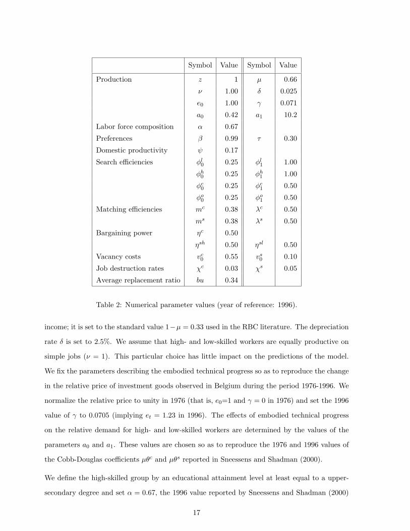
The numerical values of the parameters are reported in table 2. The reference period is the

quarter. The elasticity of output with respect to capital coincides with the capital share in total8All through the paper we assume a closed economy, while Belgium is an open economy. The assumption can

thus be thought as being restrictive. However, extending the model to an open economy would not improve its

explicative power on unemployment issues and would complicate the analysis, especially because the interest rate

would be externally fixed.

16

Symbol Value Symbol Value

Production z 1 µ 0.66

ν 1.00 δ 0.025

e0 1.00 γ 0.071

a0 0.42 a1 10.2

Labor force composition α 0.67

Preferences β 0.99 τ 0.30

Domestic productivity ψ 0.17

Search efficiencies φl0 0.25 φl

1 1.00

φh0 0.25 φh

1 1.00

φc0 0.25 φc

1 0.50

φo0 0.25 φo

1 0.50

Matching efficiencies mc 0.38 λc 0.50

ms 0.38 λs 0.50

Bargaining power ηc 0.50

ηsh 0.50 ηsl 0.50

Vacancy costs vc0 0.55 vs

0 0.10

Job destruction rates χc 0.03 χs 0.05

Average replacement ratio bu 0.34

Table 2: Numerical parameter values (year of reference: 1996).

income; it is set to the standard value 1−µ = 0.33 used in the RBC literature. The depreciation

rate δ is set to 2.5%. We assume that high- and low-skilled workers are equally productive on

simple jobs (ν = 1). This particular choice has little impact on the predictions of the model.

We fix the parameters describing the embodied technical progress so as to reproduce the change

in the relative price of investment goods observed in Belgium during the period 1976-1996. We

normalize the relative price to unity in 1976 (that is, e0=1 and γ = 0 in 1976) and set the 1996

value of γ to 0.0705 (implying et = 1.23 in 1996). The effects of embodied technical progress

on the relative demand for high- and low-skilled workers are determined by the values of the

parameters a0 and a1. These values are chosen so as to reproduce the 1976 and 1996 values of

the Cobb-Douglas coefficients µθc and µθs reported in Sneessens and Shadman (2000).

We define the high-skilled group by an educational attainment level at least equal to a upper-

secondary degree and set α = 0.67, the 1996 value reported by Sneessens and Shadman (2000)

17

for Belgium. As in most RBC models, consumers’s psychological discount factor β is set to

0.99, implying a steady state real interest rate of 0.01 (real interest rate of 4% per annum).

The domestic productivity parameter ψ is fixed at 0.17 (i.e. the domestic productivity of a

low-skilled worker is equal to 17% of the average aggregate productivity), a value which seems

reasonable and gives a realistic relative wage (wsl/wc = 62%, a value close to the relative mean

gross wage of the 33% lowest-paid full-time workers (see OECD (1996)).

Our representation of the wage determination process remains of course simplified compared to

the complexity of the Belgian system. In Belgium, there are three levels of wage negotiation:

the intra-sectoral (national) level, the sectoral level and the individual level. Every two years,

negotiations at the intra-sectoral level determine the legal minimum wage, as well as the “wage

norm”. More regularly, wage negotiations are also held within the different economic sectors

where the legal minimum wage and the wage norm are taken respectively as the lower and upper

bounds. Eventually, wages may, at each period, be (re)negotiated at the individual level. As a

consequence, in 1995, only 2% of Belgian workers were paid at the legal minimum wage. This

small percentage remains coherent with the quantitative results presented in this paper. More

precisely, following Joseph, Pierrard, and Sneessens (2004) we fix the net Katz index (defined

as the ratio of the minimum wage to the average wage) to 0.58, so that we obtain for 1996 a

minimum wage of 0.7. This value is bigger than the value associated to domestic activities,

meaning that it is always in the interest of a low-skilled worker to accept a job paid at the

legal minimum wage rather than staying at home. On the other side, we realize that the wage

earned in simple jobs equals 0.8, and whatever the shocks we introduce, it never falls below the

minimum wage (probably due to the rigidity introduced by the presence of an indexed domestic

productivity).

We have four search intensity equations, two for each segment of the labor market. We impose

identical parameter values for a given segment, which leaves four values to fix. The simple job

market search intensity coefficients have been chosen so as to normalize low-skilled workers’

search intensity to unity in 1976 and have a sensitivity to labor market tightness in the order

of magnitude estimated by Patacchini and Zenou (2003) (around 0.3). The complex market

search intensity coefficients, the disutility parameter τ , the two matching efficiency parameters

18

and the vacancy cost parameters (vc0 and vs

0) are given values to reproduce the 1996 values of

the high- and low-skilled unemployment rates (6.8% and 20.1%, respectively), the probabilities

of filling a vacant complex or simple job (qct and qs

t , around 0.4; see Delmotte, Hootegem, and

Dejonckheere (2001)) and the probabilities of finding a complex or a simple job (values pst and

pct such that the probability to find a job is around 20% for a low-skilled worker and 40% for

a high-skilled-worker; see Cockx and Dejemeppe (2004)). Our calibration of vc0 and vs

0 implies

that total vacancy costs represent 3.5% of output in the reference simulation.

We follow most authors and set the parameter determining the worker’s share in a match surplus

equal to the coefficient of unemployment in the matching function (see for instance Merz (1995)

and Andolfatto (1996))9. The latter is set at 0.5, a value obtained in many empirical estimates

of the Cobb-Douglas matching function (see Petrongolo and Pissarides (2001)) and that provides

reasonable results in our simulations. Calibrations for the average replacement ratio10 (bu =

34%) and the two job destructions rates (χc = 3% and χs = 5%) are based on estimations by

Van der Linden and Dor (2001) for the Belgian economy. A result of this calibration exercise

is that the proportion of high-skilled workers in simple jobs equals 7.3%. Even if this result

contrasts with the 24% job competition effect found in Denolf, Denys, and Simoens (2001) for

the Belgian economy, we must not forget that our theoretical setup considers job competition

only between two groups of workers: high- and low-skilled. However, as pointed by Cockx and

Dejemeppe (2004), the competition is probably more intense inside groups. Our ladder effect

under-estimates thus the true job competition effect.

3.2 Technological shocks, labor force composition and unemployment

We examine the steady state effects of three different types of shocks in order to test the

properties of the model11. First, we consider a change in labor force composition (an increase9This choice is typically motivated by the so-called Hosios-Pissarides efficiency condition. It is worth noting

that in our setup with job competition this condition may not be sufficient to ensure efficiency.10The replacement ratio is defined as the relationship between the unemployment benefits and the average labor

income.11To test the robustness of the results, we verify that the variation of every endogenous variable keeps the same

sign whatever the size of the shock introduced on the particular exogenous variable. The final size of each shock

is chosen in order to be as reasonable as possible with what seems realistic.

19

in the proportion of high-skilled in the total labor force, α). Next we look at two different

types of productivity shock (aggregate technological shock, z, and embodied technical shock,

γ). Moreover we implement a historical comparison simulation about Belgian unemployment

rates and relative wages. The results12 for the long-run effects are summarized in tables 3 to 6.

We briefly comment each exercise.

Labor force composition

A rise in the proportion of high-skilled workers in the total labor force (α) increases the prob-

ability to fill a complex job, and thus stimulates the opening of complex vacancies. The higher

number of complex jobs improves the marginal productivity of simple jobs, increasing simple

wages and stimulating search effort of low-skilled workers (elt).

Low-skilled High-skilled Low-skilled Aggregate Relative Laddersearch unemployment unemployment unemployment wage effect

efficiency rate rate rate

Benchmark simulationcorresponding to the year 1996 55.7% 7.0% 21.0% 11.7% 62.1% 7.2%

Proportion of high-skilledworkers: α = 0.67 → α = 0.70 +12.8 -0.4 -3.2 -1.6 +2.7 +2.4

Table 3: Steady state effects (deviations from the benchmark) of an increase in the proportionof high-skilled workers.

On the other side, the higher demand for simple jobs raises the probability of hiring high-skilled

workers on this type of jobs. Their search effort on the simple segment is then stimulated and

the ladder effect increases. All in all, the low-skilled unemployment rate decreases and so does

the high-skilled unemployment rate (see table 3).

Aggregate technological shock

A positive disembodied technological shock (table 4 summarizes the effects of a 5% increase in

z) raises marginal productivity of all factors. As capital cumulates, marginal productivity of12For the variables expressed in percentage, deviations from the benchmark are absolute deviations; for the

variables expressed in level, deviations from the benchmark are relative deviations.

20

complex jobs is even more stimulated via the capital-skill complementarity relationship. In spite

of the higher negotiated wages, demand for both types of jobs increases (due to the improved

productivity). All search efforts (eht, eot, elt) are thus stimulated and unemployment rates

decrease.




Total factor productivity:z = 1.00 → z = 1.05 +8.2 -0.3 -2.2 -0.9 -4.8 -1.5

Table 4: Steady state effects (deviations from the benchmark) of an increase in total factorproductivity.

Biased technological shock

Table 5 considers the effects of an embodied technological shock. The increase in γ improves

the learning efficiency of the embodied technical progress production process (from each unit

of investment the economy is able to obtain more capital than before). Capital accumulation

is then accelerated, which via capital-skill complementarity stimulates the demand for complex

jobs. This, together with the rise in complex wages, results in an increased search effort of

high-skilled unemployed (eht) and employed (eot) on the complex segment of the labor market.




Efficiency of the embodiedtechnical progress learningprocess: γ = 0.71 → γ = 0.74 -8.3 +0.2 +2.9 +1.1 -3.3 -1.3

Table 5: Steady state effects (deviations from the benchmark) of a biased technological progress.

21

The larger share of complex jobs in the production function implies a reduction in the share of

simple jobs, leading to a fall in the demand of this type of jobs as well as in their productivity.

Wages decrease and so does the search effort of low-skilled unemployed (elt). Because both

categories of workers benefit from simple jobs, a downturn in their demand affects both types of

unemployment rates. This explains the rise in high-skilled unemployment in spite of the higher

demand for complex jobs.

3.2.1 Historical comparison

The first row of table 6 reproduces the 1996 values of the proportion of high-skilled workers in

the labor force (α), the share of complex jobs in the production function (µθc), the net skill-

bias13, the high- and low-skilled unemployment rates, the relative wage (wsl/wc) and the ladder

effect. On the second row we display the change observed for these variables over the period

1976-1996.

The last two rows of table 6 contain the values predicted by the model for 1996 (benchmark

simulation) as well as the predicted variation between 1976 and 1996 when we introduce the

observed increase in the proportion of high-skilled workers and the observed rise in the decline

rate of the relative prices of new investment goods (we combine a variation in α (table 3) with

a variation in γ (table 5)). The model performs well not only in reproducing the increase in

unemployment rates, but also in maintaining relative wage rigidity.

Within the theoretical framework developed in this paper the previous results are interpreted as

follows. The post-1975 period in Belgium was characterized by an increase in the proportion of

high-skilled workers in the labor force (from 21.5% to 67%), and by the rise in the decline rate of

the investment good prices with respect to consumption prices (it attained values around -20%

during the considered period). When introducing in our model both phenomena, we observe that

the acceleration of embodied technological progress (which is at the origin of the higher decline

rate in the relative prices of investment good, 1/et) over the last decades has stimulated complex

jobs creation and simple jobs destruction, via the capital-skill complementary relationship. The13It is defined as the ratio of the relative productivity coefficient µ θc

t/(µ θst ) and the relative labor force

α/(1− α).

22

Prop. of Share complex Net High-skilled Low-skilled Relative Ladder

high-skilled jobs in the Skill unemployment unemployment wage effect

in the production Bias rate rate

labor force function

Actual data

1996 0.67 0.51 1.59 6.8% 20.1% 66% n.a.

1976-96 absolute +0.45 +0.33 +0.20 +2.1 +13.3 -0.0 n.a.

deviations

Model’s simulation

1996 0.67 0.51 1.77 7.0% 21.0% 62.1% 7.2%

1976-96 absolute +0.45 +0.32 +0.25 +2.1 +13.3 -3.4 +5.8

deviations

Table 6: Skill-bias, unemployment rates, relative wages and ladder effect in Belgium: comparingactual and simulated data.

increased demand for high-skilled workers in complex jobs has been more than satisfied by the

large upturn in their supply. In contrast, the fall in the importance of the low-skilled labor force

has not been enough to compensate the massive destruction of simple jobs and the increased

job competition. Low-skilled unemployment raises by 13.3 percentage points.

3.3 Policy scenarios

In the previous section we tested the ability of the model to reproduce the observed variations in

Belgian unemployment rates and relative wages between 1976 and 1996. This section presents

alternative historic scenarios that would have arisen if different welfare policies had been imple-

mented in 1996. Results are summarized in tables 7-11. We use the utility level of high-skilled

workers Uh = ln(Cht /α) − N sh

t D (eot) /α as an indicator of the high-skilled welfare level. In

the same way, the utility level of low-skilled, U l = ln(C lt/(1 − α)), proxies the welfare level of

this type of workers. Because the utility functions are assumed to be welfare indicators, the

attention must be focused on the variation of the value function (rather than on the specific

value of the utility function). We will compare the final welfare attained by each type of worker

under each policy context with respect to the welfare he obtained in the benchmark simulation

corresponding to 1996.

23

Tables 7-11 consider five different policy scenarios and compare them to the benchmark sim-

ulation implemented in section 3.2.1. Comparisons are implemented in a static framework,

that is, we compare the final steady states associated to each situation without considering the

transitional dynamics.

• We start analyzing a policy measure giving to firms a proportional subsidy of 20% of

low-skilled wages in 1996 (table 7), this measure being financed through a tax on high-

skilled wages. This target policy turns out to be beneficial for both, high and low-skilled

workers, in terms of unemployment reductions (this is consistent with the findings of

Pierrard (2004) for the Belgian economy). Indeed, the subsidy increases the marginal

value the firm obtains from low-skilled workers, which stimulates the opening of simple

vacancies and, thus, search efforts in the simple segment. High-skilled unemployment rates

slightly fall whereas low-skilled unemployment decreases considerably. In welfare terms,

the comparison with respect to the reference simulation, reveals that this measure mainly

favors low-skilled workers, whose welfare level clearly raises.

Prop. of Share of Net High-sk. Low-sk. Relative Ladder High-sk. Low-sk.high-skilled complex jobs Skill unempl. unempl. wage effect welfare welfare

in the in production Bias rate rate indicator indicatorlabor force function

Reference Simulation

1996 0.67 0.51 1.77 7.0% 21.0% 62.1% 7.2% 0.34 -0.20

1976-96 absolute +0.45 +0.32 +0.25 +2.1 +13.3 -3.4 +5.8 -0.25 -0.08deviations

Proportional subsidy to low wages of 20% in 1996

1996 0.67 0.52 1.80 6.8% 13.0% 71.8% 7.2% 0.33 -0.09

1976-96 absolute +0.45 +0.32 +0.29 +2.0 +5.2 +6.3 +5.7 -0.25 +0.02deviations

Table 7: Comparing the reference simulation with a scenario characterized by the presence, in1996, of a proportional subsidy to low-skilled wages of 20%.

• In table 8 we assume a situation where the replacement ratio is set to 17% (the half of its

actual value) in 1976 and 1996. This measure mainly affects low-skilled workers, whose

consumption is constrained by their revenue. Reducing the replacement ratio implies a

reduction in the reservation wage. This stimulates employment since firms can now offer

24




1996 0.67 0.51 1.77 7.0% 21.0% 62.1% 7.2% 0.34 -0.20


Replacement ratio of 17% in 1976 and in 1996

1996 0.67 0.52 1.82 5.7% 12.1% 54.3% 7.0% 0.43 -0.33


Table 8: Comparing the reference simulation with a scenario characterized by a replacementratio of 17% in 1976 and 1996.

lower wages. Both unemployment rates fall, however, only high-skilled welfare is improved,

since low-skilled workers suffer from an important loss in their revenue that results in a

downturn of their consumption level.

• Table 9 combines the two previous policy measures. This policy mix leads to a Pareto

improving situation where unemployment levels of both types of households are lower and

their welfare is improved with respect to the reference simulation. The reduced replacement

ratio stimulates employment, leading to a decrease in unemployment rates. At the same

time, the subsidy to low-skilled wages avoids the loss in the welfare suffered by unskilled

workers due to the downturn in their revenue.

• Table 10 combines a reduction in the replacement ratio to 17% during 1976-1996 and a

proportional subsidy of 4% in 1996 to low-skilled consumption financed by a tax on high-

skilled household consumption. This policy mix is also Pareto improving with respect to

the reference simulation. Unemployment rates are lower and welfare levels higher. When

comparing tables 9 and 10, we realize that subsidizing low-skilled household’s consump-

tion permits to increase their welfare by more than subsidizing their wages. However, in

this last case, unskilled unemployment rates are lower. The policy maker faces then two

possibilities:

25




1996 0.67 0.51 1.77 7.0% 21.0% 62.1% 7.2% 0.34 -0.20


Replacement ratio of 17% in 1976 and in 1996 and a subsidy to low-skilled wages of 20% in 1996

1996 0.67 0.52 1.83 5.5% 8.6% 66.6% 7.8% 0.40 -0.17

1976-96 absolute +0.45 +0.32 +0.32 +1.4 +3.1 +1.3 +6.2 -0.28 -0.03deviations

Table 9: Comparing the reference simulation with a scenario characterized by a replacementratio of 17% in 1976 and 1996 and a proportional subsidy to low-skilled wages of 20% in 1996.

1. Having most low-skilled workers employed but benefitting from a low welfare level

(subsidy to wages),

2. or having higher low-skilled unemployment rates but subsidize their consumption so

that they can benefit from a higher welfare level.




1996 0.67 0.51 1.77 7.0% 21.0% 62.1% 7.2% 0.34 -0.20


Replacement ratio of 17% in 1976 and in 1996 and a subsidy to low-skilled consumption of 4% in 1996

1996 0.67 0.52 1.83 5.7% 12.1% 54.3% 7.0% 0.41 -0.09

1976-96 absolute +0.45 +0.32 +0.31 +1.7 +6.6 -9.7 +5.4 -0.27 +0.05deviations

Table 10: Comparing the reference simulation with a scenario characterized by a replacementratio of 17% in 1976 and 1996 and a subsidy to low-skilled consumption of 4% in 1996.

• In table 11 we mix a reduction in the replacement ratio to 17% during 1976-1996 with a

subsidy of 4% to low-skilled consumption and of 20% to low-skilled wages in 1996. Putting

together the three policy measures allows to improve low-skilled workers’ situation not

26

only with respect to the benchmark simulation, but also with respect to the scenarios

developed in tables 9 and 10. Regarding high-skilled workers, even if they benefit from

lower unemployment rates, their welfare is reduced with respect to tables 9 and 10, since

now they must finance two policy measures (their wages and their consumption are taxed).




1996 0.67 0.51 1.77 7.0% 21.0% 62.1% 7.2% 0.34 -0.20


Replacement ratio of 17% in 1976 and in 1996 and a subsidy to low-skilled consumption of 4%

and to wages of 20% in 19961996 0.67 0.52 1.83 5.3% 8.6% 66.6% 7.8% 0.37 0.04

1976-96 +0.45 +0.32 +0.32 +1.4 +3.1 +2.7 +6.3 -0.31 +0.18deviations

Table 11: Comparing the reference simulation with a scenario characterized by a replacementratio of 17% in 1976 and 1996, a subsidy to low-skilled consumption of 4% and to low-skilledwages of 20% in 1996.

Of course, policies based on subsidies to low-skilled wages are, at best, effective in the short and

medium term (see Pierrard (2004)). However, in the long-run, an increase in the proportion of

skilled in the total labor force seems more appropriate. More precisely, as suggested in various

studies (see for example Cockx and Dejemeppe (2004)) a human capital investment policy would

mitigate skill mismatch and job competition (according to CESRW (2001) only 3.7% of Belgian

unemployed workers had participated in a training programme in 2000) and it would stimulate

the appearance of technological sites that develop productive activities.

4 Conclusions

Over the last 30 years, European average unemployment rates and, especially, low-skilled un-

employment rates have followed an increasing trend. Two reasons are traditionally put forward

to explain this rise: (i) the adoption of new technologies being more demanding in skilled labor,

27

combined with a rigidity in relative wages over the time, has resulted in the appearance of skill

mismatch effects; (ii) aggregate technological shocks that implied a decrease in the total labor

demand have crowded out lower educated workers by higher educated ones (job competition).

Models built up to now were unable to capture simultaneously the stylized facts observed in most

European economies: the raise in the overall unemployment rate, the more important increase in

low-skilled unemployment rates and the stability in relative wages. Our paper focuses on these

issues. We build an intertemporal general equilibrium model based on Pierrard and Sneessens

(2002) but incorporating separate wage bargaining for all workers, endogenous search intensities

and endogenous skill-biased technological progress. We calibrate it on the basis of Belgian data.

The model is then simulated to test its ability to reproduce both the situation in Belgium in 1996

and the observed variation in unemployment rates and relative wages between 1976 and 1996.

Our theoretical setup performs well in both cases. Furthermore, the model is able to reproduce

the rise in unemployment rates and the relative wage rigidity through the simple introduction of

the observed change in the proportion of high-skilled workers in the labor force and the observed

decline in the relative price of investment goods. The effects of various policy measures are also

analyzed.

Our model constitutes a successful attempt to take simultaneously into account the stylized

facts characterizing most European countries over the last decades. Two possible extensions

of the model seem quite natural. An immediate one concerns the introduction of endogenous

growth. A second extension, would consist in endogeneizing the evolution of the proportion of

high-skilled workers (α), so that the increase in low-skilled unemployment rates over the last 30

years could be explained by the introduction of skill-biased technological progress alone.

28

References

Albrecht, J., and S. Vroman. 2002. “A matching Model with Endogenous Skill Requirements.”

International Economic Review 43:283–305.

Andolfatto, D. 1996. “Business cycles and labour-market search.” American Economic Review

86 (1): 112–132.

Arrow, K. 1962. “The Economic Implications of Learning by Doing.” Review of Economic

Studies 29:155–173.

Autor, D.H., L.F. Katz, and A.B. Krueger. 1998. “Computing inequality: Have computers

changed the labour market?” Quarterly Journal of Economics 113:1169–1213.

Berman, E., J. Bound, and Z. Griliches. 1994. “Changes in the demand for skilled labor

within U.S. manufacturing: evidence from the Annual Survey of Manufacturers.” Quarterly

Journal of Economics 109:367–397.

Boucekkine, R., F. del Rio, and O. Licandro. 2002. “Embodied Technological Progress, Learn-

ing and the Productivity Slowdown.” Scandinavian Journal of Economics, vol. forthcoming.

Bresnahan, T.F., E. Brynjolfsson, and L.M. Hitt. 2002. “Information Technology, Workplace

organization, and the Demand for skilled Labor: Firm-Level Evidence.” The Quarterly

Journal of Economics 117 (1): 339–376.

Caroli, E., and J. Van Reenen. 2001. “Skilled Biased Technological Change? Evidence from

a Pannel of British and French Establishments.” Quarterly Journal of Economics 116 (4):

1449–1492.

CESRW. 2001. “Rapport sur la Situation Economique et Sociale de la Wallonie.” Conseil

Economique et Sociale de la Region Wallonne, Decembre, 118–119.

Cockx, B., and M. Dejemeppe. 2004. “Do the Higher Educated Unemployed Crowd out

the Lower Educated Ones in a Competition for Jobs?” fothcoming in Journal of Applied

Econometrics.

Collard, F., R. Fonseca, and R. Munoz. 2002. “Spanish unemployment persistence and lad-

der effect.” Centre for Economic Performance, London School of Economics and Political

Science.

29

Delmotte, J., G. Van Hootegem, and J. Dejonckheere. 2001. “Les entreprises et le recrutement

en Belgique en 2000.” HIVA, Katholieke Universiteit Leuven, and UPEDI.

Denolf, L., J. Denys, and P. Simoens. 2001. “Les Entreprises et le Recrutement en Belgique

en 2000.” HIVA, Katholieke Universiteit Leuven.

Dolado, J., F. Felgueroso, and J. Jimeno. 2000. “Youth labour markets in Spain: Education,

training and crowding-out,.” European Economic Review 44:943–956.

Dolado, J., M. Jansen, and J. Jimeno. 2002. “A matching model of crowding out and on the

job search (with an application to Spain).” mimeo.

Fitz Roy, F., and M. Funke. 1995. “Capital Skill Complementarity in West German Manufac-

turing.” Empirical Economics 20:651–665.

Forgeot, G., and J. Gautie. 1997. “Insertion Professionnelle des jeunes et processus de

declassement.” Economie et Statistique 4/5 (304-305): 53–74.

Gautier, P.A. 2002. “Unemployment and Search Externalities in a Model with Heterogeneous

Jobs and Heterogeneous Workers.” Economica 69:21–40.

Greenwood, J., Z. Hercowitz, and P. Krussel. 2002. “Long-Run Implications of Investment-

Specific Technological Change.” American Economic Review 69:21–40.

Hartog, J. 2000. “Over-education and earnings: where are we, where should we go?” Economics

of Education Review 19:131–147.

Joseph, G., O. Pierrard, and H. Sneessens. 2004. “Job Turnover, Unemployment and Labor

Market Institutions.” Labour Economics 11, no. 4.

Krusell, P., L.E. Ohanian, J.V. Rios-Rull, and G.L. Violante. 2000. “Capital skill complemen-

tarity and inequality: A macroeconomic analysis.” Econometrica 68 (5): 1029–53.

Lindquist, M. 2004. “Capital-Skill Complementarity and Inequality over the Business Cycle.”

Review of Economic Dynamics 7 (3): 519–540 (July).

Machin, S., A. Ryan, and J. Van Reenen. 1998. “Technology and changes in skill structure:

Evidence from seven OECD countries.” Quarterly Journal of Economics 113:1215–44.

Mairesse, J., G. Cette, and Y. Kocoglu. 2000. “Les Technologies de l’Information et de

30

la Communication en France: Diffusion et Contribution a la Croissance.” Economie et

Statistique 9/10 (339-340): 117–146.

Manacorda, M., and B. Petrongolo. 1999. “Skill Mismatch and Unemployment in OECD

countries.” Economica 66:181–207.

Merz, M. 1995. “Search in the labor market and real business cycle.” Journal of Monetary

Economics 36:269–300.

Moreno-Galbis, E. 2002. “Causes of the Change in the Skill Structure of the Labour Force:

An Empirical Application to the Spanish case.” IRES Dicussion Paper, no. No. 35.

Muysken, J., and B. ter Weel. 1999. “Overeducation, Job Competition and Unemployment.”

MERIT DP 99032, Maastricht University.

OECD. 1996, July. “OECD Employment Outlook.” Technical Report, OECD.

Patacchini, E., and Y. Zenou. 2003. “Search Intensity, Cost of Living and Local Labor Markets

in Britain.” IZA Discussion Paper No 772, Bonn, May.

Petrongolo, B., and C. Pissarides. 2001. “Looking Back into the Black Box: a Survey of the

Matching Function.” Journal of Economic Literature 39:390–431.

Pierrard, O. 2004. “Impacts of Selective Reductions in Labor Taxation.” mimeo. Catholic

University of Louvain.

Pierrard, O., and H. Sneessens. 2002. “Low Skilled Unemployment, Biased Technological

Change and Job Competition.” mimeo, IRES, Universite Catolique de Louvain.

Pissarides, C. 2000. Equilibrium Unemployment Theory. Edited by MIT Press. Cambridge,

Massachusetts: MIT Press.

Sneessens, H., and F. Shadman. 2000. “Analyse macro-economique des effets de reductions

ciblees des charges sociales.” Revue belge securite sociale, no. 3:613–630.

Van der Linden, B., and E. Dor. 2001. “Labor market policies and equilibrium employment:

Theory and application for Belgium.” IRES Discussion Paper. Catholic University of Lou-

vain., no. 2001-05.

31

Low-skilled unemployment, capital-skill complementarity and embodied technical progress

Documents

Transcript of Low-skilled unemployment, capital-skill complementarity and embodied technical progress