How to improve MAOR method convergence area for linear complementarity problems
Upload
khangminh22Category
view
1download
0
Diss. ETH No. 17387
The P-Matrix LinearComplementarity Problem
—Generalizations and
Specializations
A dissertation submitted to theSWISS FEDERAL INSTITUTE OF TECHNOLOGY
ZURICH
for the degree ofDoctor of Sciences
presented byLEONARD YVES RUST
M.Sc. ETH in Computer Scienceborn March 23, 1980
citizen of Thal (SG), Switzerland
accepted on the recommendation ofProf. Dr. Emo Welzl, ETH Zurich, examinerDr. Bernd Gartner, ETH Zurich, co-examiner
Prof. Dr. Hans-Jakob Luthi, ETH Zurich, co-examinerProf. Dr. Walter D. Morris, Jr., George Mason University,
Fairfax, co-examiner
2007

II

Abstract
The goal of this thesis is to give a better understanding of the linearcomplementarity problem with a P-matrix (PLCP). Finding a polyno-mial time algorithm for the PLCP is a longstanding open problem. Suchan algorithm would settle the complexity status of many problems re-ducing to the PLCP. Most of the papers dealing with the PLCP lookat it from an algebraic point of view. We analyze the combinatorialstructure of the PLCP.
Wherever possible, we state our results for the generalized PLCP(PGLCP), a natural generalization of the PLCP. In the first part of thethesis, we present further generalizations of the PGLCP. We show thatthe PGLCP fits into the framework of unique sink orientations (USO)of grids. Finding a solution to the PGLCP can therefore be done byfinding the sink in a grid USO. Several algorithms are known for thislatter task, and we analyze the behavior of some of them on small grids.We thereby make use of the result that PGLCP-induced USOs fulfill acombinatorial property known as the Holt-Klee condition.
Grid USOs are then shown to fit into the framework of violatorspaces. Violator spaces have been introduced as a generalization of LP-type problems capturing the combinatorics behind many problems likelinear programming or finding the smallest enclosing ball of a pointset. We prove that Clarkson’s algorithms, originally developed for low-dimensional linear programs, work for violator spaces that in contrastto LP-type problems have a cyclic structure in general. This yields anoptimal linear time algorithm for solving PGLCP with a fixed numberof blocks.
III

The second part of the thesis deals with specializations of the PGLCP.We first focus on a subclass of P-matrices, known as hidden K-matrices.The hidden K-matrix PGLCP is known to be solvable in time polyno-mial in the input size. We give an alternative proof for this fact andstrengthen it by the following statement: the USO arising from a hiddenK-matrix PGLCP is LP-induced and therefore always acyclic. Further-more, a nontrivial and large subclass of non hidden K-matrices is given,and we prove that the PLCP with a 3-dimensional square P-matrix inthis class reduces to a cyclic USO in general.
Our last result is that simple stochastic games (SSG) can be refor-mulated as PGLCP. People have unavailingly been trying to show thatgames like SSG are polynomial-time solvable for over 15 years. Theconnection to PGLCP gives us powerful tools to further attack this.Unfortunately, SSG do in general not reduce to PGLCP with a matrixin a known polynomially solvable class.
IV
Zusammenfassung
Das Ziel dieser Dissertation ist es, das lineare Komplementaritatsprob-lem mit einer P-Matrix (PLCP) besser zu verstehen. Einen Algorith-mus zu finden der das PLCP in polynomieller Zeit lost ist ein seit langemoffenes Problem. So ein Algorithmus wurde den Komplexitatsstatusvieler Probleme festlegen, die auf das PLCP reduzierbar sind. In denmeisten Arbeiten uber das PLCP wird es von einer algebraischen Sicht-weise analysiert. Im Gegensatz dazu schauen wir uns die kombina-torische Struktur des PLCP genauer an.
Wann immer moglich formulieren wir unsere Resultate fur das ver-allgemeinerte PLCP (PGLCP), eine naturliche Verallgemeinerung desPLCP. Im ersten Teil dieser Arbeit prasentieren wir eine weitere Ve-rallgemeinerung des PGLCP. Wir zeigen dass das PGLCP formuliertwerden kann als das Problem, die eindeutige Senke einer eindeutige-Senke-Orientierung (USO) eines Gitters zu finden. Wir schauen unsdas Verhalten einiger Algorithmen fur das USO-Problem auf kleinenGittern an. Dabei benutzen wir das Resultat, dass die USO, die voneinem PGLCP stammen, die Holt-Klee Eigenschaft haben.
Danach zeigen wir, dass USO auf Gittern wiederum verallgemeinertwerden konnen, und zwar auf Verletzer-Raume. Diese wurden als Ver-allgemeinerung von Problemen, die ahnlich wie lineares Programmieren(LP) sind, eingefuhrt und haben eine zyklische zugrunde liegende Struk-tur. Wir beweisen, dass die bekannten LP-Algorithmen von Clarksonauf Verletzer-Raume angewandt werden konnen und erhalten so einenoptimalen Algorithmus, der das PGLCP mit einer fixen Anzahl Blockenin linearer Zeit lost.
V

Im zweiten Teil dieser Dissertation befassen wir uns mit Spezial-isierungen des PGLCP. Zuerst schauen wir uns eine Unterklasse von P-Matrizen an, bekannt als versteckte K-Matrizen. Das PGLCP mit einerversteckten K-Matrix kann mittels LP gelost werden. Wir geben einenalternativen Beweis fur diese Aussage und starken sie zudem wie folgt:die USO die aus dem PGLCP mit einer versteckten K-Matrix resul-tiert stammt von einem LP und ist deshalb azyklisch. Zudem definierenwir eine neue Unterklasse von Matrizen die nicht versteckt K sind undzeigen, dass das PLCP mit 3-dimensionalen quadratischen P-Matrizenin dieser Klasse im Allgemeinen in einer zyklischen USO resultiert.
Unser letztes Resultat ist, dass einfache stochastische Spiele (SSG)als PGLCP formuliert werden konnen. Seit uber 15 Jahren versuchtman zu zeigen, dass SSG in polynomieller Zeit gelost werden konnen.Die von uns aufgezeigte Verbindung zum PGLCP gibt neue und machtigeWerkzeuge um dieses Ziel weiter zu verfolgen. Leider reduziert sich dasSSG im Allgemeinen auf PGLCPs mit Matrizen die zu keiner bekanntenpolynomiell losbaren Klasse gehoren.
VI

Acknowledgments
My deepest gratitude goes to my advisor Bernd Gartner who mademy PhD possible. He was there whenever I needed advice and helpedme out of many dead ends. All my papers are co-authored by him andwithout his broad knowledge, they would not have reached their quality.Thanks for all your support!
A big thank you goes to Emo Welzl for letting me be part of hisresearch group and for his uncomplicated and upright manner, makingthe time at ETH unforgettable.
I thank my co-referees Hans-Jakob Luthi for reviewing this thesisand sharing the passion for the LCP and Walter D. Morris for reviewing,supporting me over the years via e-mail and the joint paper.
The following people made it a pleasure to work at ETH:
Robert Berke, Yves Brise, Tobias Christ, Kaspar Fischer, HeidiGebauer, Jochen Giesen, Franziska Hefti, Michael Hoffmann, MartinJaggi, Shankar Lakshminarayanan, Andreas Meyer, Dieter Mitsche,Yoshio Okamoto, Andreas Razen, Dominik Scheder, Eva Schuberth,Ingo Schurr, Milos Stojakovic, Marek Sulovsky, Tibor Szabo, PatrickTraxler, Floris Tschurr, Elias Vicari, Uli Wagner, Frans Wessendorp,Philipp Zumstein. Moreover all the members from the other researchgroups at our institute and, of course, the 22 red and blue guys on theH-floor.
Further a big thank you to the following people:
My co-authors Jirka Matousek and Petr Skovron for interesting
VII

meetings and the joint paper.
Markus Brill, Matus Mihal’ak, Rahul Savani, Alex Souza-Oftermattand the A-Team for an incredible time in Denmark.
Aniekan Ebiefung, Nir Halman, Klaus Simon, Roman Sznajder, OlaSvensson, Takeaki Uno, Bernhard von Stengel for inspiring discussions.
My family and all of my friends outside ETH for always being there.
My wife for loving me and my boys for tearing me away from thecomputer and trying to convince me that playing tag is more importantthan writing a thesis.
VIII
Contents
Abstract III
Zusammenfassung V
Acknowledgments VII
1 Introduction 1
1.1 Overview . . . . . . . . . . . . . . . . . . . . . . . . . . 1
1.2 Short Outline of the Thesis . . . . . . . . . . . . . . . . 11
1.3 The P-Matrix Linear Complementarity Problem . . . . 13
Part I: Generalizations 19
2 The P-Matrix Generalized LCP 21
2.1 The Setup . . . . . . . . . . . . . . . . . . . . . . . . . . 21
2.2 Π-Compatible Linear Programming . . . . . . . . . . . . 25
3 Unique Sink Orientations 29
3.1 Reduction from PGLCP to Grid USO . . . . . . . . . . 30
IX

3.2 The Holt-Klee Condition . . . . . . . . . . . . . . . . . . 34
3.3 Ladders . . . . . . . . . . . . . . . . . . . . . . . . . . . 36
4 Violator Spaces 59
4.1 LP-Type Problems . . . . . . . . . . . . . . . . . . . . . 59
4.2 The Violator Space Framework . . . . . . . . . . . . . . 62
4.3 Clarkson’s Algorithms . . . . . . . . . . . . . . . . . . . 65
4.4 Grid USO as Models for Violator Spaces . . . . . . . . . 72
Part II: Specializations 77
5 Hidden K-Matrices 79
5.1 Matrix Classes . . . . . . . . . . . . . . . . . . . . . . . 81
5.2 Hidden K-Matrix GLCP and LP . . . . . . . . . . . . . 85
5.3 Non Hidden K-Matrices . . . . . . . . . . . . . . . . . . 95
6 Simple Stochastic Games 107
6.1 The Setup . . . . . . . . . . . . . . . . . . . . . . . . . . 108
6.2 Reduction from SSG to PGLCP . . . . . . . . . . . . . 110
6.3 Negative Results . . . . . . . . . . . . . . . . . . . . . . 117
Bibliography 129
Curriculum Vitae 139
X
Chapter 1
Introduction
Against widespread belief, the abbreviation LCP does not stand forLeo’s Core Problem but for the Linear Complementarity Problem. How-ever, the former interpretation of the abbreviation is true for sure. Thisthesis collects results achieved during the author’s PhD studies, all ofwhich nicely connect to the LCP. It is based on three papers [33, 31, 34],their journal versions [32, 30] and unpublished material (for exampleSection 3.3 or Chapter 5).
The next section gives a detailed overview about our work and aboutwhat has been done and known before. It describes which of our resultshave been published where, with whom (all results are published to-gether with Bernd Gartner, so only different co-authors are mentionedbelow) and with what differences to the thesis at hand. The hurriedreader looking for specific results might prefer the condensed overviewgiven in Section 1.2.
1.1 Overview
Although special instances of the LCP first appear in a paper by Du Valalready in 1940 [23], intensive analysis started in the mid 1960’s wherealso the name linear complementarity problem originated. One of the
1
2 Chapter 1. Introduction
earliest applications is that the first-order optimality conditions of aquadratic program can be written as an LCP [43, 1]. Besides countlessother applications – a small but significant selection is for example givenin [80] – there are also connections to game theory: bimatrix games allowan LCP formulation [15, 95]. We show in this thesis that other gameslike simple stochastic games can be reduced to the LCP as well.
The most comprehensive sources for the LCP are the books [17]by Cottle, Pang, and Stone and [67] by Murty. The LCP is givenby linear equations, described by a square matrix M ∈ R
n×n and aright-hand side vector q ∈ R
n, and nonnegativity conditions as well ascomplementarity conditions. More concretely, given M and q, it is tofind vectors w ∈ R
n and z ∈ Rn such that
w −Mz = qw, z ≥ 0wT z = 0,
or to show that no such vectors exist.
Many relevant applications reduce to an LCP where M has specialproperties. A lot of research has been done on various matrix classes, aclassical paper is [26] and a rich collection of results about matrix classesand their connections to the LCP can be found in [17]. We focus on theclass of P-matrices. A matrix is a P-matrix if the determinants of allprincipal submatrices are positive. This class is interesting because it isknown that the LCP has a unique solution for every q if and only if thematrix is a P-matrix [79]. Applications for the P-matrix LCP (PLCP)can be found for example in [7, 80, 77, 20].
It has been shown by Megiddo that hardness of the PLCP would im-ply that NP = co-NP [58]. Despite this fact, no polynomial algorithmis known up to date. Finding such an algorithm is one of the majorgoals of the LCP community since it would settle the complexity statusof many problems reducing to the PLCP. One of the main LCP algo-rithms is the one from Cottle and Dantzig [15]. It is a principal pivotalgorithm, pivoting from one basis of the LCP to the next according toa specified pivot-rule. The behavior of principal pivot algorithms hasbeen investigated for many different pivot-rules, see [17] in general or[66, 27] for a nice appetizer.
Another important algorithm for the LCP is the one given by Lemke
2

1.1. Overview 3
in [50]. Remarkably, the Lemke-Howson algorithm, which is a variantof Lemke’s algorithm tailored for LCPs arising from bimatrix games,is an efficient constructive procedure for obtaining mixed equilibriumstrategies for bimatrix games [51]. This constituted the simplest andmost elegant constructive proof for the existence of Nash equilibria inbimatrix games (Nash’s previous proof was based on the nonconstruc-tive Brouwer fixed point theorem [68, 69]).
Besides the classical algorithms by Lemke and Cottle and Dantzig,there are still new ones being developed, see for example [38] for amore recent one. Interior point algorithms are also known, describedfor instance in [49]. Each of the above mentioned algorithms worksfor a larger class of matrices than P-matrices. See the references fordiscussions about termination depending on the matrix class.
We tackle the PLCP from two sides in this thesis. On the one hand,we show in the first part of this work that it fits into more general, easilystructured frameworks. Although the generalizations are proper, andwe therefore lose information, the simplicity of the frameworks allowsfor an improvement of algorithm running time. In fact, the fastestknown algorithms solving PLCP were developed for these frameworks.On the other hand, we describe two specializations in the second partof this thesis. We first look at a subclass of P-matrices and examine thecombinatorial structure behind the LCP associated with these matrices.The second specialization is actually a new application for the PLCP.We reduce a game theory problem to the PLCP. The relations betweenthe frameworks and problem classes discussed in this thesis are depictedat the end of this section in Figure 1.2 on page 11.
Generalized linear complementarity problems. The first gener-alization we look at is the generalized linear complementarity problemwith a P-matrix (PGLCP) in Chapter 2. The PGLCP was introducedby Cottle and Dantzig in [16]. It is more general than the PLCP sincethe matrix M is not restricted to be square. The matrix in the GLCP isa vertical block matrix to which the notion of P-matrix can be extended.The important properties of the PLCP generalize to the PGLCP: theGLCP has a unique solution for every right-hand side vector q if andonly if its matrix is a P-matrix (see [16, 90, 39] or also [37]), and hard-ness of the PGLCP would imply NP = co-NP (this is easy to provealong the lines in [58]). In our paper [33, 32], we state the PGLCP and
3

4 Chapter 1. Introduction
correlated results in a form dual to the one of Cottle and Dantzig. Inthis thesis, we mostly stick to the original setting of Cottle and Dantzig,but we explain the dual setting in Section 2.2, revealing connections tolinear programming (LP). These connections are useful to derive resultsabout the PGLCP with the special matrix class described in Chapter 5.
Unique sink orientations of grids. In Chapter 3 we then presentour result from [33, 32], that the PGLCP fits into the framework ofunique sink orientations of grids. A grid is a graph whose vertex setis the Cartesian product of finite sets, with edges joining all pairs ofvertices that differ in exactly one component. Alternatively, we canview a grid as the skeleton (vertex-edge graph) of a specific polytope,namely a product of simplices. If all sets have size two, which is the caseif we reduce the PLCP, we get the graph of a cube. A face or subgridis any induced subgraph spanned by the Cartesian product of subsetsof the original sets. An orientation ψ of the grid is called a unique sinkorientation (USO) if every face has a unique sink with respect to ψ.USOs can in general be cyclic.
A polynomial-time algorithm for finding the sink of a grid USO (us-ing an oracle that returns the orientation of a given edge) would solvethe PGLCP in strongly polynomial time. Candidates for strongly poly-nomial algorithms must be combinatorial in the sense that the numberof arithmetic operations they perform depends only on the combinato-rial structure of the PGLCP but not on the actual numbers that encodeit.
Most of the papers dealing with PLCP or PGLCP analyze the prob-lem from an algebraic point of view. With the USO approach we shedmore light on the combinatorial structure of the PGLCP. First effortsin this direction have been made by Stickney and Watson [87], who con-sidered orientations of cubes as digraph models for PLCP. Although thename USO was formed only later in [89], their orientations are in factUSOs. Stickney and Watson give an example of a PLCP resulting in acyclic 3-dimensional cube USO. Morris constructed highly cyclic PLCP-induced USOs in higher dimensions for which the algorithm followinga random outgoing edge at every cube-vertex performs very badly [64].Most remarkably, Szabo and Welzl gave algorithms for finding the sinkof any n-cube USO by looking at only O(cn) vertices and edges, for somec strictly smaller than 2 [89]. This in particular yields the first combina-
4

1.1. Overview 5
torial algorithms for PLCP with nontrivial runtime bounds. For acycliccube USO, Gartner gives a subexponential algorithm in [28]. CubeUSO are useful as combinatorial models for many other problems, see[89, 33, 32] and references therein for more detailed discussions.
The generalization from PGLCP to grid USO reveals some (algo-rithmically useful) hidden structure, leading to new results for PGLCP.Since most of these results were already derived in the author’s Masterthesis [78], we present only the actual reduction from PGLCP to gridUSO in Chapter 3. In [33, 32] we presented the result that PGLCP-induced grid USOs satisfy the Holt-Klee condition. The Holt-Klee con-dition is a combinatorial property shared by a diminishing fraction of allUSO [22]. The fraction of PGLCP-induced grid USOs is even smaller,since there are Holt-Klee grid USOs that do not come from PGLCP[63].
The problem of finding an optimal sink-finding algorithm can bestated as a zero-sum game which in turn can be solved by linear pro-gramming [29]. Unfortunately, the LP gets too big already for smallgrid USOs. In the last section of Chapter 3, Section 3.3, we analyzea subclass of 2-dimensional grids called ladders. Ladders are the sim-plest grid USO for which we don’t know optimal algorithms. For smallenough ladders, by making use of isomorphisms as described in [91], theLP whose solution encodes an optimal algorithm is solvable in reason-able time. We describe optimal algorithms derived this way for smallladders. These give us an intuition how optimal algorithms might be-have on general ladders. At the end of Chapter 3, we give an almostoptimal algorithm for ladders satisfying the Holt-Klee condition. Ourfindings about ladders have not been published.
Violator spaces. A further result, motivated by our ambition to an-alyze the combinatorics behind the PGLCP, is the generalization fromgrid USOs to violator spaces in Chapter 4. Violator spaces are propergeneralizations of LP-type problems. The framework of LP-type prob-lems, invented by Sharir and Welzl in 1992 [84], was used to show thatLP is solvable in subexponential time in the RAM model (independentof the precision of the input numbers) [57].
Violator spaces were introduced by Jirka Matousek and Petr Skovronin [85]. In this thesis, we present results derived together with them in
5

6 Chapter 1. Introduction
our joint paper [31, 30]. The reason we look at violator spaces is thatLP-type problems have an acyclic structure, which prevents generalgrid USOs (in particular PGLCP-induced cyclic ones) to fit into thisframework. To our knowledge, violator spaces are, besides orientedmatroid programs (see for example [6]), the only abstract optimizationframework allowing cycles. We prove that grid USOs, and thereforePGLCPs, are subsumed by violator spaces.
Section 4.3 shows that Clarkson’s randomized algorithms [11], de-veloped for low-dimensional LP (they are also applicable to LP-typeproblems, see [35, 9]) work in the context of violator spaces. These al-gorithms give us an optimal linear time algorithm for the PGLCP witha constant number of blocks. More results about violator spaces can befound in [85, 86, 31, 30], for example that LP-type problems and acyclicviolator spaces are equivalent.
Hidden K-matrices. Chapter 5 is dedicated to the PGLCP withhidden K-matrices, a proper subclass of P-matrices that also appearsunder the name hidden Minkowski matrices or mime matrices (see [93]).Hidden K-matrices show up in real world problems, for example theproblem of pricing American put options can be solved with the help ofa hidden K-matrix LCP [7] (more precisely, the matrix belongs to theeven smaller subclass of K-matrices). The theory behind the hidden K-matrix GLCP was founded by Mangasarian in his papers [52, 53, 54, 55].Mangasarian analyzed GLCPs that can be restated as linear programs.Cottle and Pang extended research in this direction [19, 18, 72, 71, 70],finally ending up with the main result that the hidden K-matrix LCPcan be solved by linear programming and therefore in time polynomialin the input size [47] (see also the strongly polynomial time algorithmsfor matrices whose transpose is hidden K [73, 62]). This was generalizedto the GLCP by Mohan and Neogy in [61].
We strengthen the hidden K theory by showing that the grid USOwe get from the hidden K-matrix GLCP is an orientation we get froman LP. The USO is therefore acyclic for any right-hand side vector q.In an attempt to characterize those non hidden K but P-matrices thatyield a cyclic orientation for some q (we call such a q a cyclic q), wefirst derive a characterization for matrices that are not hidden K. Ourcharacterization generalizes the characterization of [65] to the GLCPcase. We then introduce a new nontrivial and large subclass of non
6

1.1. Overview 7
hidden K-matrices and prove that 3-dimensional P-matrices in this classhave a cyclic q. However, we fail to prove this for higher dimensions. Itthus remains an open problem to characterize those P-matrices havinga cyclic q. None of our results about the hidden K-matrix GLCP hasbeen published yet.
Simple stochastic games. The last chapter of the thesis is aboutsimple stochastic games. Simple stochastic games (SSG) form a subclassof general stochastic games, introduced by Shapley in 1953 [83]. Condonwas first to study the complexity-theoretic aspects of SSG [12]. Sheshowed that the decision version of the problem is in NP∩ co-NP. Thisis considered as evidence that the problem is not NP-complete, becausethe existence of an NP-complete problem in NP ∩ co-NP would implyNP = co-NP. Despite this evidence and a lot of research, the questionwhether a polynomial time algorithm exists remains open. This remindsus of the PGLCP, whose hardness would also imply NP = co-NP andfor which no polynomial time algorithm is known. Indeed, we presentin Chapter 6 our result from [34] that SSG can be reduced to PGLCP.
A SSG is played by moving a token on a directed graph whose ver-tex set consists of two sinks, the 0-sink and the 1-sink, and the restpartitioned into three parts, vertices belonging to the max player, minplayer, and average vertices, respectively. At a vertex, the player it be-longs to chooses along which outgoing edge to move the token. The goalof the max player is to (maximize the probability to) reach the 1-sink,the goal of the min player to reach the 0-sink. We consider SSG withvertices of arbitrary outdegree and with average vertices determiningthe next vertex according to an arbitrary probability distribution. Thisis a natural generalization of binary SSG introduced by Condon [12].As a specialization of the results in Chapter 6 we get that a binary SSGreduces to the PLCP.
SSG are significant because they allow polynomial-time reductionsfrom other interesting classes of games. Zwick and Paterson proved areduction from mean payoff games [98] which in turn admit a reduc-tion from parity games, a result of Puri [75]. See the references forapplications of these games.
A strategy of a player determines for every vertex belonging to theplayer along which outgoing edge to move the token. Given a strategy
7

8 Chapter 1. Introduction
of one player, the optimal counterstrategy of the other player can becomputed by a linear program [21]. Using this, Halman could show thatthe problem of finding an optimal strategy for one of the players can bestated as an LP-type problem [41] (see also [42, 40]) and can thereforebe solved in strongly subexponential time.
Independently, Bjorklund et al. arrived at subexponential methodsby showing that SSG can be mapped to the combinatorial problem ofoptimizing a completely local-global function over the Cartesian productof sets [3]. This setup is the same as the setup of acyclic grid USOs,which can in turn be formulated as LP-type problems. In fact, they findthe sink of the acyclic USO by applying LP-type algorithms, so theirapproach is actually equivalent to Halman’s.
The methods of Halman and Bjorklund et al. focus on the strat-egy of one player while recomputing the optimal counterstrategy of theother player in every step. By solving the SSG via PGLCP we do notdistinguish between the two players. This is best explained in the USOworld. An algorithm following an outgoing edge in a grid USO inducedby an SSG via the PGLCP formulation improves the strategy of theplayer the “edge belongs to”. The dimension of the grid is the num-ber of player vertices in the SSG and an edge along dimension i in thegrid is associated with player vertex i. Following one edge in the USOsetting means to switch the strategy of one player at one vertex in thegame. Condon [13] (see also the example in Subsection 6.3.1) shows thatswitching algorithms can cycle, so the underlying USO can be cyclic.This is not the case in the setting of Bjorklund et al. Their USO iswith respect to one player, the max player, say, so the dimension ofthe grid is the number of vertices of the max player. Every vertex inthe grid corresponds to a strategy of the max player, and a grid-vertexevaluation, returning the orientations of incident edges, is achieved bycomputing the optimal counterstrategy of the min player. An edge inthe grid is outgoing, if the strategy at the neighboring grid-vertex isbetter for the max player. This implies that the grid USO is acyclic.
In [78, 33] we introduced the concept of projected (or inherited)grid USOs. Roughly, a projected grid USO is derived by merging setsof vertices along a subset of the grid’s dimensions into single verticesand taking the outgoing edges of the sink in the set of original verticesmerged into one to be the outgoing edges of the resulting vertex. Onecan show that this is again a (smaller dimensional) grid USO. See Fig-
8

1.1. Overview 9
Figure 1.1: A 3-dimensional grid USO and a projected grid USO of itderived by merging vertices along one dimension.
ure 1.1 for an example. If, in the grid USO derived from an SSG viaPGLCP, all dimensions corresponding to one player are merged, thenthe resulting grid USO is exactly the one from Bjorklund et al. andtherefore acyclic. This is a very special property, which we don’t expectfrom general PGLCP-induced USO. This is the reason why we thinkthat PGLCP is more general than SSG, meaning that it is not possibleto get every P-matrix in the reduction from SSG to PGLCP.
Nevertheless, by looking at a superclass of SSG, derived from SSG byadding payoff-values to the edges, our reduction may yield any right-hand side vector q in the PGLCP (changing the payoffs changes theq-vector but does not affect the matrix). Shapley’s stochastic gamesstill contain this superclass of SSG and Shapley’s theorem [83] provinguniqueness of game values then implies that the GLCP has a uniquesolution for every q and its matrix must therefore be a P-matrix. Ourresult that the matrix in the reduction is a P-matrix thus provides analternative proof of Shapley’s theorem, specialized to SSG, and it makesthe connection to matrix theory explicit.
There are interesting connections between algorithms in the USOsetting and algorithms for the SSG. The algorithm bottom-antipodal inthe USO world, for example, being at vertex v jumps to the vertexantipodal in the face spanned by all the outgoing edges of v. There areexponential lower bounds for the performance of this algorithm [82]. Wecan interpret the behavior of bottom-antipodal in SSG. In the settingof Bjorklund et al. it means that given a strategy for the max player,simultaneously switch the strategy at every max vertex that has a switchimproving the strategy. Then compute the optimal counterstrategy of
9

10 Chapter 1. Introduction
the min player and proceed as before. This algorithm is a variant of theHoffman-Karp algorithm for SSG [44, 13].
The fact that there is a connection between games and LCP is notentirely surprising, since, as noted in the beginning of this section, forexample bimatrix games can be formulated as LCP [15, 95]. Also Cottle,Pang and Stone [17, Section 1.2] list a simple game on Markov chains asan application for LCP, and certain (very easy) SSG are actually of thetype considered. Bjorklund et al. describe a reduction from games towhat they call controlled linear programming [4]; controlled linear pro-grams are easily mapped to (non-standard) LCP. Independently fromour work, Bjorklund et al. have made this mapping explicit by derivingLCP-formulations for mean payoff games [5]. Their reduction is verysimilar to ours, but the authors do not prove that the resulting matricesare P-matrices, or belong to some other known class. In fact, Bjorklundet al. point out that the matrices they get are in general not P-matrices,and this stops them from further investigating the issue. We have a sim-ilar phenomenon here: applying our reduction to non-stopping SSG, wemay also obtain matrices that are not P-matrices. The fact that comesto our rescue is that the stopping assumption incurs no loss of general-ity and, in contrast to our paper [34], we make heavy use of it in thisthesis, simplifying the reduction a lot. For mean payoff games, a similarresult holds. They can without loss of generality be transformed intodiscounted mean payoff games [98]. Jurdzinski and Savani [45] couldprove that reducing discounted mean payoff games results in LCP witha P-matrix.
Our result that SSG-induced GLCPs come with P-matrices puts SSGinto the realm of ‘well-behaved’ GLCP, but it does not give improvedruntime bounds. Unfortunately, the matrices we get from SSG do ingeneral not belong to a class known to be polynomial-time solvable, seeSection 6.3. Still, properties of the subclass of matrices we ask for mightallow their PGLCP to be solved in polynomial time. By, without lossof generality, simplifying the graph underlying the SSG first, Svenssonand Vorobyov managed to reduce SSG to PGLCP with a very simplystructured matrix [88]. However, no progress has been made so far inalgorithmically exploiting this structure.
10

1.2. Short Outline of the Thesis 11
PSfrag replacements
Violator Spaces
Grid USO
LP-Type Problems
PGLCP
PGLCP
PLCP
Hidden K
SSG
Figure 1.2: An overview of the classes used in this thesis.
1.2 Short Outline of the Thesis
In the next section, we define the linear complementarity problem andintroduce the necessary notations. After that, the thesis is split intotwo parts. In the first part we present three generalizations of thePLCP, the first being the P-matrix generalized linear complementarityproblem (PGLCP) in Chapter 2. Most of the chapter is consumed bydefinitions and setting notation, but we also provide a dual view ofthe PGLCP which we introduced in our paper together with Walter D.Morris [33, 32], making visible connections to linear programming.
The second generalization described in Chapter 3 is that of uniquesink orientations (USO). We show, in a different setting than the onewe used in [33, 32], how the PGLCP reduces to finding the sink of aUSO on a grid graph. Moreover, we review the Holt-Klee condition, acombinatorial property shown to hold for PGLCP-induced grid USO in[33, 32]. The chapter ends with a detailed presentation of unpublishedresults about special instances of grid USOs, which we call ladders.
11

12 Chapter 1. Introduction
These are the simplest grid USOs for which we don’t know the optimalalgorithms. We give an almost optimal algorithm to find the sink in aHolt-Klee ladder.
The third generalization is that of violator spaces. Violator spacesform a framework subsuming LP-type problems, a framework inventedby Sharir and Welzl [84]. We show in Chapter 4 that grid USOs (andtherefore the PGLCP) are models for violator spaces but not for LP-type problems in general. Moreover, Clarkson’s algorithms, that havebeen designed for low dimensional linear programs and later adapted forLP-type problems, are shown to work for violator spaces. This yields anoptimal linear time algorithm for solving PGLCP with a fixed numberof blocks. These results, together with some structural results aboutviolator spaces, are published in [31, 30]. This is joint work with JirkaMatousek and Petr Skovron.
In the second part we look at specializations of the PLCP. In Chap-ter 5 we consider LCPs associated with a subclass of P-matrices: hiddenK-matrices. Altough being in the specialization part here, we look atthe hidden K-matrix generalized LCP whenever possible. The mainachievement is a proof that the USO arising from a hidden K-matrixGLCP is LP-induced and therefore always acyclic. Additionally, we at-tempt to characterize those matrices from which a cyclic USO arisesand succeed to define a nontrivial and large subclass of 3-dimensionalnon hidden K-matrices that give rise to a cycle. The material in thischapter has not been published yet.
The final Chapter 6 extends our results from [34]. Using a simplersetting than in the paper, we show how simple stochastic games canbe reduced to the PGLCP. This makes the whole PGLCP machineryavailable for games. We further give some negative results, for examplethat the resulting matrix in the PGLCP is not hidden K in general.
12

1.3. The P-Matrix Linear Complementarity Problem 13
1.3 The P-Matrix Linear Complementarity
Problem
Given a matrix M ∈ Rn×n and a vector q ∈ R
n, the linear complemen-tarity problem (LCP) is to find a vector z ∈ R
n such that
z ≥ 0q +Mz ≥ 0
zT (q +Mz) = 0(1.1)
or to show that no such vector exists. In this thesis, we use an oftenencountered equivalent formulation of the LCP, that will simplify ouranalysis in later chapters: given a matrix M ∈ R
n×n and a vectorq ∈ R
n, the LCP is to find vectors w ∈ Rn and z ∈ R
n such that
w −Mz = qw, z ≥ 0wT z = 0
(1.2)
or to show that no such vectors exist. We refer to (1.2) as LCP(M, q).Note that the nonnegativity conditions w, z ≥ 0 together with the com-plementarity condition wT z = 0 force at least one of the variables wiand zi to be zero for all i ∈ {1, . . . , n}.
We are interested in the LCP(M, q) where M is a P-matrix.
Definition 1.3 A matrix M ∈ Rn×n is a P-matrix if the determinants
of all principal submatrices are positive.
We refer to determinants of principal submatrices as principal minors.The relevance of the LCP with a P-matrix, abbreviated as PLCP, stemsfrom the following theorem, first proved in [79].
Theorem 1.4 The LCP(M, q) has a unique solution for all vectors q ∈Rn if and only if M ∈ R
n×n is a P-matrix.
Beauty and simplicity of the PLCP are best explained in the geometricview. In order to be able to do this, we first need some notation. Wedenote by [n] the set of integers from 1 to n. Given matrix A ∈ R
n×n
13

14 Chapter 1. Introduction
and a set α ⊆ [n], the matrix Aα ∈ Rn×|α| is derived by deleting those
columns from A whose indices are not in α. For readability, we letAα := A[n]\α. The same notation is applied to n-vectors, with theobvious meaning. Moreover, for B ∈ R
n×n we define (Aα||Bα) ∈ Rn×n
to be the matrix whose ith column is A{i} if i ∈ α and B{i} otherwise.The same definition analogously holds for vectors, so given a ∈ R
n and
b ∈ Rn, the ith component of
(aα
bα
)
is ai if i ∈ α and bi otherwise. To
make the reader more familiar with this notation, we give an examplefor n = 3. Let
A :=
1 2 31 2 31 2 3
, B :=
4 5 64 5 64 5 6
,
and
a :=
123
, b :=
456
.
Then
(A{1,3}||B{2}) =
1 5 31 5 31 5 3
and
(a{1,3}b{2}
)
=
153
.
There are 2n possibilities to satisfy the complementarity condition inthe PLCP, achieved by setting either wi or zi to zero in each coordinatei. As soon as we fix the complementary set of variables that should be
zero, say the variables(wα
zα
)
for some α, then the values of the remaining
variables(wα
zα
)
are uniquely determined: pre-multiplying the PLCP
with (Iα|| − Mα)−1 (note that existence of the inverse easily followsfrom the fact that M is a P-matrix) results in
(wαzα
)
−M ′
(wαzα
)
= (Iα|| −Mα)−1q
for M ′ := −(Iα||−Mα)−1(Iα||−Mα). Since(wα
zα
)
are the zero variables,
we get(wα
zα
)
= (Iα|| −Mα)−1q.
14

1.3. The P-Matrix Linear Complementarity Problem 15
Definition 1.5 A subset α ⊆ [n] is called a basis of the PLCP (1.2),and
B(α) := (Iα|| −Mα)
is the corresponding basis matrix.
A basis α determines that the variables wα and zα are set to zero.Taking into account the nonnegativity constraints for w and z, solving
the PLCP is equivalent to finding a basis α ⊆ [n] for which(wα
zα
)
=
B(α)−1q ≥ 0. We often say that such an α is a solution to the PLCP,since w and z are derived immediately from it.
The procedure of computing M ′ = −B(α)−1B(α) from M as aboveis known as a principal pivot transform, abbreviated as PPT. Tuckerfirst proved that a matrix derived from a P-matrix via a PPT is again aP-matrix [94]. A PPT corresponds to rewriting the PLCP with variableswi and zi interchanged for some indices i ∈ [n].
This thesis deals with nondegenerate PLCPs only. A PLCP is de-generate if B(α)−1q has a zero entry for some α and it is nondegenerateotherwise. Nondegeneracy can easily be achieved by slightly perturbingthe vector q, such that for all α, B(α)−1q has no zero entries. For a solu-tion α, this implies that all nonzero variables are positive, B(α)−1q > 0.Moreover, there is a unique set α for which B(α)−1q > 0, since two dif-ferent sets fulfilling the condition would imply two different solutions(because different variables are nonzero in the two solutions) to thePLCP, contradicting Theorem 1.4. We come back to the nondegener-acy issue in the geometric view of the PLCP which we describe now.
The 2n basis matrices of the PLCP can be interpreted as n-dimen-sional cones in R
n, called complementary cones. For any α, the com-plementary cone associated with B(α) is spanned by the n vectors cor-responding to the columns of B(α) (since B(α) is non-singular, thosecolumns are linearly independent). Finding the unique α such thatB(α)−1q > 0 is then to find the unique complementary cone whichcontains the vector q. Since the PLCP has a unique solution for all q(Theorem 1.4), the complementary cones cover the whole space. More-over, they intersect only in lower dimensional cones, since otherwise, a qlying in the interior of a full dimensional intersection would be containedin two distinct complementary cones (contradicting the uniqueness of
15

16 Chapter 1. Introduction
������������������������������������������������������������������������������������������������������������������������������������������������������������������������������������������������������������������������������������������������������������
������������������������������������������������������������������������������������������������������������������������������������������������������������������������������������������������������������������������������������������������������������
���������������������������������������������������������������������������������������������������������������������������������������������������������������������������������������������������������������������������������������
���������������������������������������������������������������������������������������������������������������������������������������������������������������������������������������������������������������������������������������
� � � � � � �� � � � � � �� � � � � � �� � � � � � �� � � � � � �� � � � � � �� � � � � � �� � � � � � �
� � � � � � �� � � � � � �� � � � � � �� � � � � � �� � � � � � �� � � � � � �� � � � � � �� � � � � � �
PSfrag replacements
(10
)
(01
)
(−1−1
) (0−1
)
(−112
)
= q
Figure 1.3: Geometric view of the PLCP (1.6).
the basis α with B(α)−1q > 0). As an example for the geometric view,look at the PLCP
1 0
0 1
w1
w2
−
1 0
1 1
z1
z2
=
−1
12
w1, w2, z1, z2 ≥ 0
w1 · z1 + w2 · z2 = 0
(1.6)
whose geometric view is given in Figure 1.3. From the picture we seethat q lies in the complementary cone spanned by the columns of thebasis matrix B({2}). The variables w1 and z2 are therefore zero andthe positive values of the variables z1 and w2 can be computed as
(w{2}
z{1}
)
=
(z1w2
)
= B({2})−1q =
(−1 0−1 1
)−1( −112
)
=
(132
)
.
16

1.3. The P-Matrix Linear Complementarity Problem 17
If q is contained in a hyperplane that contains the (n− 1)-dimensionalintersection of two complementary cones, then the PLCP is degenerate.Let B(α) and B(α′) correspond to two complementary cones whose(n−1)-dimensional intersection is contained in a hyperplane containingq as well. Since the intersection of the two cones is (n− 1)-dimensional,α and α′ differ only in one element, i.e., their symmetric differenceis 1: |α ⊕ α′| = |{i}| = 1. Although the solution to the PLCP is stillunique, the complementary cone containing q might not be unique sinceB(α)−1q and B(α′)−1q are zero at coordinate i and possibly positivein all other coordinates. In order to get rid of such cases, we perturbq a little bit, i.e., we move it slightly such that it is no more containedin any hyperplane containing the intersection of two complementarycones. This affects the solution to the PLCP in a controllable way(variables that are zero in the original setting can have arbitrarily smallsolution values in the perturbed setting) and for the rest of this thesis wetherefore stick to the assumption of nondegeneracy, i.e., (B(α)−1q)i 6= 0for all α and i. In particular, B(α)−1q > 0 for the solution α.
17

18 Chapter 1. Introduction
18

Part I: Generalizations
In this first part of the thesis we present three generalizations of thePLCP, the first being the generalized linear complementarity problem(PGLCP) in Chapter 2. We define the notation needed for the PGLCPand also state the problem in the dual setting we used in [33, 32]. Allfurther results, if possible, are then stated for the PGLCP.
Chapter 3 shows how PGLCP can be reduced to unique sink orien-tations (USO) of grids. In [33, 32] we showed that these orientationsfulfill a well-known combinatorial property, the Holt-Klee condition. Atthe end of this chapter, the Holt-Klee condition is useful in the analysisof algorithms for the smallest class of grid USOs for which no optimalalgorithms are known.
The last chapter in this part introduces violator spaces as a furthergeneralization of grid USOs (and therefore PGLCP). Violator spacesform a simple combinatorial framework, and our result that Clarkson’salgorithms work for them yields an optimal linear time algorithm forsolving PGLCPs of fixed dimension.
19

20

Chapter 2
The P-Matrix
Generalized LCP
The generalized linear complementarity problem, abbreviated as GLCP,was introduced by Cottle and Dantzig in 1970 [16]. It generalizes theLCP(M, q) by dropping the requirement of M being a square matrix.
2.1 The Setup
In order to state the GLCP, we first define the type of a matrix.
Definition 2.1 A matrix G is a vertical block matrix of type (g1, . . . , gn)if it is of the form
G =
G1
...Gn
where the ith block Gi, i ∈ [n], has order gi × n.
21

22 Chapter 2. The P-Matrix Generalized LCP
For reasons that will become clear in the next chapter, we define N tobe
N :=n∑
i=1
gi + n,
i.e., G is an (N−n)×n matrix. The definition of a vertical block matrixapplies in a straightforward way also to vectors.
Given a vertical block matrix G ∈ R(N−n)×n and a vertical block
vector q ∈ RN−n, both of type (g1, . . . , gn), the GLCP is to find a
vertical block vector w ∈ RN−n of type (g1, . . . , gn) and a vector z ∈ R
n
such thatw −Gz = q
w, z ≥ 0
zi
gi∏
j=1
wij = 0, for all i ∈ [n].(2.2)
In analogy to Gi, wi is the ith block of size gi of the vector w. In theGLCP, complementarity holds block-wise, i.e., either zi is zero or atleast one variable in the block wi. We refer to (2.2) as GLCP(G, q).
Definition 2.3 A representative submatrix G ∈ Rn×n of G is derived
by letting the ith row of G be one row out of the block Gi for all i ∈ [n].
There are∏ni=1 gi different representative submatrices of G. With their
help, the P-matrix notion can be generalized to vertical block matrices.
Definition 2.4 A vertical block matrix G ∈ R(N−n)×n is a vertical
block P-matrix if all principal minors of all representative submatricesare positive.
So, every (square) representative submatrix of a vertical block P-matrixis itself a P-matrix (as defined in Definition 1.3). We sometimes omitthe words “vertical block” when it is clear from the context what kindof matrix we mean. Cottle and Dantzig show that a solution to theP-matrix GLCP always exists [16], and Szanc shows in his dissertationthat the solution is unique for all q [90, 39], so Theorem 1.4 generalizesto the GLCP.
22

2.1. The Setup 23
Theorem 2.5 The GLCP(G, q) has a unique solution for all vectorsq ∈ R
N−n if and only if G ∈ R(N−n)×n is a P-matrix.
We abbreviate the P-matrix GLCP by PGLCP. For our analysis, it willbe easier to restate the PGLCP in the following form. Let I be theidentity matrix in R
(N−n)×(N−n) and divide it into n blocks of columnswith the ith block having size (N−n)×gi. Now expand the ith block byappending −G{i}, the negated ith column of G. The resulting matrixH1 is of order (N −n)×N and consists of n blocks of columns with theith block having size (N − n) × (gi + 1). The first gi columns of blocki are the ones from I and the last column is −G{i}. The same is donewith the vectors w and z. A new vector x ∈ R
N is formed from w byappending zi to the bottom of wi. The first gi components of block xi
are therefore the components of wi and the last component of xi is zi.Finally, in order to simplify notation, we set hi := gi + 1 for all i andrewrite the PGLCP (2.2) as
Hx = qx ≥ 0
hi∏
j=1
xij = 0, for all i ∈ [n].(2.6)
We refer to this setting as PGLCP(H, q). In this form, it is easier todefine bases for the PGLCP. The partition ofH into n blocks of columnscorresponds to a partition Π of [N ] into n subsets Πi of size hi each,
Π = (Π1, . . . ,Πn).
Let β ⊆ [N ] be an n-element set consisting of one element out of eachΠi, i = 1, . . . , n. Such a set is called representative and the elementin β belonging to Πi is denoted by βi. There are
∏ni=1 hi many rep-
resentative sets β. To shortcut notation, we set β := [N ] \ β. Then,Hβ ∈ R
(N−n)×(N−n) is the matrix H restricted to columns whose in-dices are not in β.
Definition 2.7 A representative subset β ∈ [N ] is called a basis of thePGLCP(H, q), and
B(β) := Hβ
1Since the matrix is a mixture of −G and I, it seems appropriate to choose theletter which lies between G and I in the alphabet.
23

24 Chapter 2. The P-Matrix Generalized LCP
is the corresponding basis matrix in R(N−n)×(N−n).
We also define xβ to be the vector x restricted to elements with indicesnot in β. More precisely, the ith block of xβ is the ith block of x reducedby the element with index βi in x.
The elements of β correspond to the variables in x that are set to zerosuch that complementarity is fulfilled. Once β is fixed, the remainingvariables are determined, since the PGLCP(H, q) can be pre-multipliedby B(β)−1 (nonsingularity of B(β) comes out ofG’s P-matrix property):
B(β)−1Hx = H ′x = B(β)−1q
with H ′β
being the identity matrix in R(N−n)×(N−n) and H ′
β being a
vertical block matrix −G′. Setting xβ to zero then yields xβ = B(β)−1q.
The matrix G′ is derived from the original matrix G via a principalpivot transform. Habetler and Szanc generalized Tucker’s result thatsquare P-matrices are closed under PPT to vertical block P-matrices[39]. The matrix G′ is thus a vertical block P-matrix.
As in the PLCP case, solving the PGLCP amounts to finding theβ for which B(β)−1q > 0, where we again assume that the PGLCP isnondegenerate. Note that the geometric point of view can also be takenin the PGLCP. Any basis matrix can be interpreted as an (N − n)-dimensional complementary cone in R
(N−n) and Theorem 2.5 makessure that these cones cover the whole space and intersect only in lowerdimensional cones. The same considerations about nondegeneracy asfor the PLCP apply, and we therefore assume for the rest of the thesisnondegeneracy of the PGLCP.
The cone point of view will be important in Section 3.2, where westate the result derived in [33, 32] that the orientation implicitly under-lying a PGLCP (described in the next section) satisfies a special prop-erty. But first we devote a section to the description of the PGLCP inthe dual setting we used in [33, 32], revealing connections to the linearprogramming problem.
24

2.2. Π-Compatible Linear Programming 25
2.2 Π-Compatible Linear Programming
Consider a linear program (LP) in the variables x = (x1, . . . , xN )T , ofthe form
minimize cTxsubject to Ax = b
x ≥ 0,(2.8)
where A ∈ Rn×N , b ∈ R
n and c ∈ RN . The index set [N ] of A’s columns
is partitioned into n blocks by Π = (Π1, . . . ,Πn). As in the previoussection, let β be a representative set consisting of exactly one elementper block Πi. Assume that for all β, Aβ is a nondegenerate basis matrixin (2.8), meaning that Aβ is invertible and A−1
β b > 0. We say that theLP is Π-compatible, and we call Aβ a representative submatrix. We willassume that the ordering of the columns in Aβ is compatible with Π,meaning that the i-th column of Aβ comes from AΠi
, i ∈ [n].
Using Cramer’s rule, the following is not hard to establish.
Observation 2.9 Consider a Π-compatible LP of the form (2.8). Then
(i) all determinants det(Aβ) of representative submatrices have thesame (nonzero) sign, and
(ii) the Aβ are the only basis matrices of the LP (2.8).
Proof. Let the n× n basis matrices Aβ and Aβ′ differ in one column,column i. Then, by Cramer’s rule, the ith component of the solution toAβxβ = b and Aβ′xβ′ = b respectively, is given by
(xβ)i =det(Aiβ)
det(Aβ), (xβ′)i =
det(Aiβ′)
det(Aβ′),
where the matrix Aiβ is Aβ with the ith column replaced by the vec-tor b which is the same as Aβ′ with the ith column replaced by b.Since xβ > 0 for all β, we get that sign(det(Aβ)) = sign(det(Aiβ)) =
sign(det(Aiβ′)) = sign(det(Aβ′)). This proves (i).
For (ii), assume that there is a basis matrix Aγ ∈ Rn×n for a non-
representative set γ, so A−1γ b > 0. For the time being, assume that γ
25

26 Chapter 2. The P-Matrix Generalized LCP
has its first two elements out of block Π1, no element out of block Π2
and exactly one element out of every other block. Cramer’s rule thentells us that
det(A1γ)
det(Aγ)> 0,
det(A2γ)
det(Aγ)> 0.
So sign(det(A1γ)) = sign(det(A2
γ)). Note that det(A2γ) = det(A2
β) for
some representative set β and det(A1γ) = − det(A2
β′) for some other
representative β′ (by swapping the first two columns in A1γ), imply-
ing sign(det(A2β)) 6= sign(det(A2
β′)). This is a contradiction since by
Cramer’s rule and (i) we have sign(det(A2β)) = sign(det(A2
β′)). Thus,
Aγ is not a basis matrix and sign(det(A1γ)) 6= sign(det(A2
γ)) must hold.Using this, we can pivot to the next γ (for example the one having twoelements in the first and third block, none in the second and fourth, andone element in the other blocks) and derive a contradiction by the samearguments as above. Pivoting to all non-representative sets γ proves(ii). �
If A fulfills condition (i) of Observation 2.9, we say that A has propertyP.
For any c ∈ RN , a canonical Π-compatible LP is obtained by setting
bi = 1 and
Aij :=
{1, j ∈ Πi
0, otherwise, i ∈ [n], j ∈ [N ].
In this case, all representative submatrices are equal to the n-dimensionalidentity matrix, and the feasible region is the product of n simplices,where the i-th simplex is defined in the space of variables xj , j ∈ Πi,via the constraints ∑
j∈Πi
xj = 1, xj ≥ 0.
The LP dual to (2.8) is
maximize bT ysubject to yTA ≤ cT .
(2.10)
Since (2.8) is Π-compatible, an optimal solution x∗ fulfills x∗β > 0 forsome representative set β. By complementary slackness (see for exam-ple [56]), the constraints corresponding to this set β in yTA ≤ cT arefulfilled with equality in an optimal solution to (2.10).
26

2.2. Π-Compatible Linear Programming 27
By dropping the requirement that (2.8) is Π-compatible, but stillinsisting on A to have property P, we get the following more generalproblem: given matrix A with property P and vector c, find a vectory ∈ R
n such thatcT ≥ yTA, (2.11)
and with the property that for every i ∈ [n], there is a j ∈ Πi satisfying
cj = (yTA)j . (2.12)
We refer to this problem as PGLCP*(A, c), since, according to the fol-lowing lemma, it is a dual form of the PGLCP.
Lemma 2.13 Let A ∈ Rn×N and c ∈ R
N such that A has propertyP. The PGLCP*(A, c) is equivalent to a PGLCP, in the sense that asolution to one problem yields a solution to the other.
Proof. Given the PGLCP*(A, c) withA partitioned by Π = (Π1, . . . ,Πn),fix a representative set β and define
GT := A−1β A,
qT := cT − cTβA−1β A.
G is a vertical block P-matrix of type (|Π1|, . . . , |Πn|) which easily fol-lows from the fact that GT has property P and contains a representativeidentity submatrix. We look at the following PGLCP:
w −Gz = q (2.14)
w, z ≥ 0 (2.15)∏
j∈Πi
wj = 0, i ∈ [n]. (2.16)
Since the z-variables do not appear in the complementarity condition(2.16), this is actually not a proper PGLCP. But by definition, qβ = 0and (GT )βi = ei for βi being the unique element in β ∩Πi and ei ∈ R
n
being the i-th unit vector. Consequently, every solution to (2.14) mustsatisfy zi = wβi for i ∈ [n]. This means that (2.16) may be replacedwith
zi∏
j∈Πi
wj = 0, i ∈ [n],
27

28 Chapter 2. The P-Matrix Generalized LCP
making the PGLCP proper.
Given a solution w, z to this PGLCP, a solution y to the PGLCP* isgiven by yT = (cTβ−zT )A−1
β . This is because (2.14) gives wT = cT−yTAand conditions (2.15) and (2.16) then ensure that y is as desired.
Vice versa, given a PGLCP(G, q) we enhance G ∈ R(N−n)×n by a
representative identity submatrix and q accordingly by n zero entriesat coordinates corresponding to the representative identity submatrix.Given a solution y to the PGLCP* with A := GT and c := q, a solutionw, z to the (enhanced) PGLCP is given by zT = −yT and wT = cT −yTA. �
Intuitively, PGLCP* is LP of the form (2.8) ’without a right-handside’ and therefore a generalization of Π-compatible linear program-ming. The generalization is proper, because given a PGLCP* instance(A, c), it is not always possible to find a right-hand side b such thatA, b, c form a Π-compatible LP. We prove this in Chapter 5, where weshow that b exists if and only if the matrix G, constructed from A as inthe proof above, belongs to the class of hidden K-matrices.
28
Chapter 3
Unique Sink Orientations
The term unique sink orientation (USO) first appears in a paper bySzabo and Welzl [89]. There, a USO is an edge-orientation of the n-dimensional hypercube such that every face/subcube of the cube has aunique sink (a vertex with all edges within the subcube incoming). Inthe author’s Master thesis, this concept has been generalized to orien-tations of grids (to be defined shortly) and it has been shown that thePGLCP can be mapped to finding the unique sink of a grid USO [78].This result, which was later published as part of [33, 32], is a generaliza-tion of the work of Stickney and Watson [87], who reduced the PLCPto unique sink orientations of cubes.
We show the reduction from PGLCP to grid USO in the setting (2.6)that is different from the setting in [33, 32] (where we used the PGLCP*setting of Section 2.2), but more natural in the context of this thesis.We review the Holt-Klee condition in Section 3.2, and at the end of thischapter we devote a section to the analysis of special 2-dimensional gridUSOs which we call ladders. We describe an optimal algorithm to findthe sink in a ladder of size 3 and an almost optimal algorithm to findthe sink in a Holt-Klee ladder of general size.
29

30 Chapter 3. Unique Sink Orientations
PSfrag replacements(
10
)
Figure 3.1: The 3-dimensional grid([N ],Π) with N = 7 and Π =({1, 2, 3}, {4, 5}, {6, 7}) and a USO of it.
3.1 Reduction from PGLCP to Grid USO
An n-dimensional grid is given by a partition Π = (Π1, . . . ,Πn) of someground set [N ] into n blocks. We consciously use the same letters Π, Nand n as in the PGLCP(H, q), since the PGLCP with (N−n)×N matrixH , partitioned into blocks of columns according to Π = (Π1, . . . ,Πn),reduces to an n-dimensional grid defined by [N ] and Π.
Definition 3.1 The n-dimensional grid([N ],Π), spanned by the set [N ]and a partition Π = (Π1, . . . ,Πn) of it with |Πi| ≥ 2 for all i, is theundirected graph G = (V , E) with
V := {V ⊆ [N ]: |V ∩ Πi| = 1, i = 1, . . . , n},E := {{V, V ′} ⊆ V : |V ⊕ V ′| = 2}.
The vertices naturally correspond to the Cartesian product of the Πi.The edges in E connect vertices/sets in V that differ in exactly onecomponent. Every vertex therefore has (N − n) neighbors. See Fig-ure 3.1 left for an example of a grid. We ask for |Πi| ≥ 2 in the defini-tion of the grid([N ],Π), since a block Πi∗ of size one, holding elementj say, results in a smaller dimensional grid that is equivalent to thegrid([N \ j], (Π1, . . . ,Πi∗−1,Πi∗+1, . . . ,Πn)).
Every subset F ⊆ [N ] defines a vertex induced subgrid(F,Π) of thegrid([N ],Π) by restricting to vertices V ∈ V for which V ⊆ F (we shouldactually also restrict Π to act only on elements of F , but for notational
30

3.1. Reduction from PGLCP to Grid USO 31
simplicity we ask the reader to keep this in mind and leave it as it is).The subgrid(F,Π) is the empty graph whenever F ∩ Πi = ∅ for somei. We say that such an F is not Π-valid, and it is Π-valid otherwise.A nonempty subgrid(F,Π) has less dimensions than the grid([N ],Π) if|F ∩ Πi| = 1 for some i ∈ [n].
Definition 3.2 An edge-orientation ψ of the grid([N ],Π) is called aunique sink orientation (USO) if all nonempty subgrids have uniquesinks w.r.t. ψ.
Grid USOs can in general be cyclic, see Figure 3.1 right for an example.All 2-dimensional grid USOs are acyclic [33, 32], so the smallest cyclicgrid USO is the one given in Figure 5.2 on page 92. The orientationgiven in Figure 3.1 right is special, since it is a smallest cyclic grid USOwith all subcube USOs being acyclic.
We now show how to reduce the PGLCP to grid USO. The repre-sentative sets β in the PGLCP naturally correspond to the vertices Vin the grid. There is an edge between vertex β and β ′ if and only if βand β′ differ in exactly one component that belongs to a block Πi, soβi 6= β′
i. This is in turn the case if and only if, up to reshuffling columns,the basis matrices B(β) and B(β′) differ in exactly one column. Moreprecisely, there is a column with index iββ′ in B(β) and a column withindex iβ′β in B(β′), such that removing column iββ′ from B(β) resultsin the same matrix as removing column iβ′β from B(β′). Note thatiββ′ = iβ′β if and only if βi = β′
i ± 1.
An orientation ψ of this grid graph is derived according to the fol-lowing rule, where the notation
β′ ψ→ β
denotes that the orientation ψ induces the edge directed from β ′ to β:
β′ ψ→ β ⇔ (B(β)−1q)iββ′ > 0. (3.3)
In the simpler PLCP setting, where bases and basis matrices are definedaccording to Definition 1.5, this can equivalently be stated as
α′ ψ→ α ⇔ (B(α)−1q)i > 0, (3.4)
31

32 Chapter 3. Unique Sink Orientations
where α⊕ α′ = {i}.
Theorem 3.5 The grid-orientation ψ induced by the PGLCP via (3.3)is a unique sink orientation.
Proof. Since the PGLCP has a unique solution β that fulfillsB(β)−1q >0, β is the global unique sink with all (N − n) edges incoming. It thusremains to show that every proper subgrid has a unique sink, which wedo by showing that the orientation of each subgrid is again PGLCP-induced. Since edges are subgrids, this also proves that each edge isdirected into exactly one direction, so
(B(β)−1q)iββ′ > 0 ⇔ (B(β′)−1q)iβ′β< 0.
Fix a nonempty subgrid(F,Π), F ⊆ [N ], and let β be any ver-tex in it. We pre-multiply the PGLCP(H, q) by B(β)−1 and get thePGLCP(H ′, q′). This is a principal pivot transform, transforming theP-matrix G underlying H into P-matrix G′ underlying H ′, as discussedat the end of Section 2.1. The PPT rearranges the variables. The gridorientation arising via (3.3) from the transformed PGLCP is isomor-phic to the original one. The orientation in the subgrid(F,Π) is theninduced by the PGLCP derived as follows. For all j ∈ [N ] \ F deletethe corresponding column in H ′. This column is zero in all entries ex-cept one, where it is 1 (that’s the reason we did the PPT). Delete therow from H ′ that contains this 1 and delete the corresponding entryin q′. The deleted row contains the information how xj is determinedin terms of the other x-variables and a constant in q′. Since xj doesnot appear in any other equation, the orientation induced by the re-sulting (non-standard) sub-GLCP coincides with the orientation of thesubgrid([N ] \ j,Π) (because at every basis common to the PGLCP andthe sub-GLCP, the x-variables different from xj have the same valuesin the PGLCP as in the sub-GLCP).
The sub-GLCP might be non-standard because we might end upwith only one column in a block, but we need two columns per blockfor the complementarity condition to make sense. After deletion of allcolumns in [N ] \F and the corresponding rows from H ′, the remainingmatrix is a merging of an identity matrix and a matrix G′′, derived fromG′ by deleting rows. If there is only one column left in one block (whichmust be a column of G′′ corresponding to a vertical block in G′ that
32

3.1. Reduction from PGLCP to Grid USO 33
has been erased completely), it can be deleted since the correspondingvariable has to be zero by the complementarity condition. This resultsin a standard GLCP. And the fact that G′ is a P-matrix immediatelyimplies that G′′ is a P-matrix. �
The PLCP is a special case of the PGLCP where every block of thematrix H consists of two columns. Or, in the setting (2.2), every blockof G has one row. The reduction thus works for the PLCP, too, in whichcase the grid is a cube.
Thanks to the reduction, finding the solution to a PGLCP is equiv-alent to finding the sink of a grid USO. Indeed, the fastest algorithmsknown to solve PLCP as well as PGLCP are sink-finding algorithms.We refer the reader to the literature for descriptions and analysis ofalgorithms working for general cube [89] and grid [33, 32] USOs. Ournew contribution in this direction is the development of new algorithmsfor some special classes of grid USOs in Section 3.3. Moreover, the ap-plication of the violator space framework described in Chapter 4 resultsin a fast algorithm for fixed-dimensional grid USOs.
An interesting problem is to characterize USOs that are PGLCP-induced. Acyclicity is not required, since there are examples of PLCPsthat reduce to cyclic USOs [87]. But it is known [33, 32], that PGLCP-induced grid USOs have a simple property known as the Holt-Klee con-dition. Before we look at this condition, we define the outmap of a gridUSO, a concept which we will need in later sections.
Any USO can be specified by associating each vertex V with itsoutgoing edges. Given V and j ∈ [N ] \ V , we define V B j to be theunique vertex V ′ ⊆ V ∪ {j} that is different from V , and we call V ′ theneighbor of V in direction j. Note that V is a neighbor of V ′ in somedirection different from j.
Definition 3.6 Given an orientation ψ of the grid graph G = (V , E)determined by the set [N ] and its partition Π, the function sψ : V →2[N ], defined by
sψ(V ) := {j ∈ [N ] \ V :Vψ→ V B j}, (3.7)
is called the outmap of ψ.
33
34 Chapter 3. Unique Sink Orientations
��
������
����
������
��
Figure 3.2: The forbidden non-HK subgrid USOs up to dimension 3.
By this definition, any sink w.r.t. ψ has empty outmap value.
3.2 The Holt-Klee Condition
A set of directed paths from the unique source to the unique sink ofa grid USO is called vertex-disjoint if no two of the paths share anyvertices other than the source or sink. A proof that a grid USO hasa unique source can be found in [33, 32]. We say that a grid USO isHolt-Klee (HK) if the following definition applies.
Definition 3.8 A grid USO satisfies the Holt-Klee condition if thereare as many vertex-disjoint paths from the unique source to the uniquesink as there are neighbors of the source, and if in addition, everynonempty subgrid USO satisfies the Holt-Klee condition.
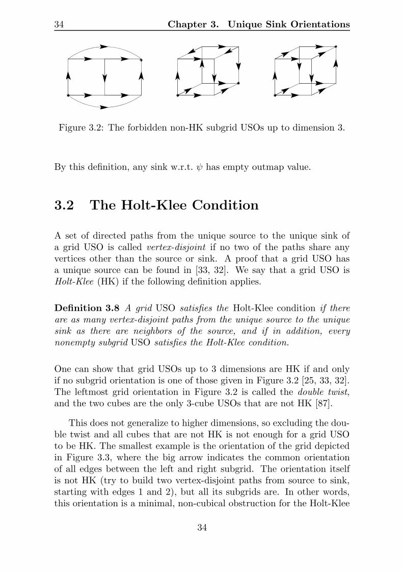
One can show that grid USOs up to 3 dimensions are HK if and onlyif no subgrid orientation is one of those given in Figure 3.2 [25, 33, 32].The leftmost grid orientation in Figure 3.2 is called the double twist,and the two cubes are the only 3-cube USOs that are not HK [87].
This does not generalize to higher dimensions, so excluding the dou-ble twist and all cubes that are not HK is not enough for a grid USOto be HK. The smallest example is the orientation of the grid depictedin Figure 3.3, where the big arrow indicates the common orientationof all edges between the left and right subgrid. The orientation itselfis not HK (try to build two vertex-disjoint paths from source to sink,starting with edges 1 and 2), but all its subgrids are. In other words,this orientation is a minimal, non-cubical obstruction for the Holt-Klee
34

3.2. The Holt-Klee Condition 35
PSfrag replacements1
2
Figure 3.3: A minimal non HK 4-dimensional grid USO.
condition in dimension n = 4. The example can be extended to yield aminimal non-cubical obstruction in any dimension n ≥ 4.
An open question is whether there is a finite family of forbiddensubgrid orientations for given n whose absence makes any n-dimensionalgrid USO HK.
Let’s go back to the cone point of view of the PGLCP. Rememberthat the columns of basis matrices B(β) of PGLCP(H, q) span comple-mentary (N − n)-dimensional cones. Further, the existence of a uniquePGLCP solution for all q implies that these cones cover the whole spaceand that the intersection of two complementary cones is a lower di-mensional cone. The dual graph underlying the cone point of view isderived by interpreting the (N − n)-dimensional complementary conesas vertices. Two vertices are joined by an edge if the corresponding com-plementary cones intersect in a (N−n−1)-dimensional cone. This dualgraph is exactly the grid graph we get in the reduction from PGLCP togrid USO.
In a nondegenerate PGLCP, q is in general position, meaning that itis not contained in any hyperplane containing a (N−n−1)-dimensionalintersection of two complementary cones. If a vector q is in generalposition, we can define an orientation of the dual graph, in which an
35

36 Chapter 3. Unique Sink Orientations
edge joining the neighboring complementary cones K and K ′ is orientedfrom K to K ′ if K \K ′ and q are on opposite sides of the hyperplanecontaining K∩K ′. The digraph derived that way has a unique sink andsource, which are the cones containing q and −q. In [33, 32] we presentedthe proof that these orientations fulfill the Holt-Klee condition. Sinceresults in [33, 32] are derived in the PGLCP* setting (see Section 2.2),we give a short argument why the orientation defined in Section 3.1through Equation (3.3) is in fact the same as the one of the dual graphjust described.
The neighboring complementary cones K and K ′ are spanned bythe columns of the basis matrices B(β) and B(β ′), respectively. Up toreshuffling columns, B(β) differs from B(β ′) only by the column withindex iββ′ in B(β) (as discussed in the previous section). The vectorsq and B(β){iββ′} (corresponding to K \K ′) lie on opposite sides of the
hyperplane containing the cone spanned by the columns shared by B(β)and B(β′) (corresponding to K ∩K ′) if and only if (B(β)−1q)iββ′ < 0.PGLCP-induced grid USOs defined through (3.3) therefore fulfill theHolt-Klee condition.
The fact that PGLCP-induced USOs are HK might be exploited bysink-finding algorithms. In the next section, we design such an algo-rithm for 2-dimensional grids with one dimension fixed to size 2.
3.3 Ladders
The work in this section evolved from a problem posed at the 2ndGremo’s Workshop on Open Problems (GWOP) 20041. We abstractfrom the PGLCP and focus on the problem of finding a sink in a gridUSO.
A USO is usually implicitly given through a vertex evaluation ora-cle that returns for any given vertex the orientations of the incidentedges. An optimal algorithm finding the sink in the 1-dimensionalgrid([N ], (Π1)) can easily be seen to need expected HN vertex evalu-ations, where HN is the Nth harmonic number: the runtime of thebest deterministic algorithm on the input of uniformly at random dis-
1http://www.ti.inf.ethz.ch/ew/workshops/gwop04/
36

3.3. Ladders 37
tributed USOs can be computed to be HN expected vertex evaluations.By Yao’s Principle [96], this is a lower bound for the expected worst-case runtime of the best randomized algorithm. Since the randomizedalgorithm that follows a random outgoing edge needs expected HN ver-tex evaluations (independent of the USO distribution), HN is optimalin the 1-dimensional grid.
For general grid USO, two sink finding algorithms have been pre-sented in [33, 32]. Here, we specialize to s-ladders, 2-dimensional gridswith one block of size 2 and the other of size s. By the previous dis-cussion, this is the simplest nontrivial case of a (non-cubic) grid (see[89] for algorithms for cube USOs). The goal of this specialization isto reuse gained knowledge in higher dimensional grids and to show howHK can be exploited.
This section is structured as follows. After the formal definitionof ladders, we analyze the behavior of a simple but general grid USOalgorithm on them. Then a specific algorithm for ladders is given whichseems to make a lot of sense but surprisingly turns out to be slowerthan the simple algorithm. Finally, we present an optimal algorithm forfinding the sink in a 3-ladder and a nearly optimal algorithm for HKladder USOs.
Definition 3.9 The s-ladder Ls is the 2-dimensional grid([s + 2],Π)with Π = (Π1,Π2), |Π1| = 2 and |Π2| = s.
See Figure 3.4 for the example L4 with 4 steps. In general, Ls con-sists of two complete graphs on s vertices where each vertex in one ofthese graphs is connected with exactly one in the other graph. Theseconnections form the s steps of the ladder.
For the PGLCP, a vertex evaluation oracle can be implemented torun in time polynomial in the size of the matrix H : returning the orien-tations of the edges incident to vertex β amounts to computingB(β)−1q.In case of a ladder, B(β) is a square matrix of dimension s.
37

38 Chapter 3. Unique Sink Orientations
Figure 3.4: The ladder L4 with 4 steps.
3.3.1 Simple Algorithms
Let’s first analyze how the product algorithm, developed for generalgrids in [33, 32], behaves on ladders. It removes a random step ofthe ladder and recursively evaluates the sink of the resulting subladderLs−1. In case this sink is not yet the global sink (its unique incidentedge connecting it to the removed step will tell), the global sink is inthe removed step. This happens with probability 1/s, and to find thesink of the step, 3/2 evaluations suffice on average. We therefore getthe recurrence
t(s) = t(s− 1) +3
2s, (3.10)
with t(0) = 0, for the expected total number of vertex evaluations. Thisyields
t(s) =3
2Hs, s ≥ 0.
Knowing that the sink of L2 (the 2-cube) can be found with an expectednumber of 43/20 vertex evaluations (this is optimal) [89], we can slightlyimprove the product algorithm by using
t(2) =43
20
as a base of the recurrence. This yields
t(s) =3
2Hs −
1
10, s ≥ 2. (3.11)
Another approach to construct an algorithm is via a property of gridUSO. Specialized to ladder USO, it says that for every pair (i, j), 0 ≤i < 2, 0 ≤ j < s, there is exactly one vertex with i outgoing vertical
38

3.3. Ladders 39
edges and j outgoing horizontal edges [33, 32]. The pair (i, j) is therefined index of that vertex.
Choose one vertex v at random. If its refined index is (0, j), then avertex like v′ in Figure 3.5 can not be the sink, since that would resultin v and v′ both being sinks in the 2-cubical face spanned by them. Theglobal sink is therefore in the subladder Lj spanned by the j steps thatcontain the neighbors of v along its j outgoing edges, see Figure 3.5.Thus, we recursively evaluate the sink of this subladder and are done.If j = 0, the subladder is empty and v itself is the global sink.
PSfrag replacements
· · ·
· · ·
Lj
v
v′
Figure 3.5: Case 1: v has refined index (0, j); the global sink is in thesubladder Lj (or equals v if j = 0).
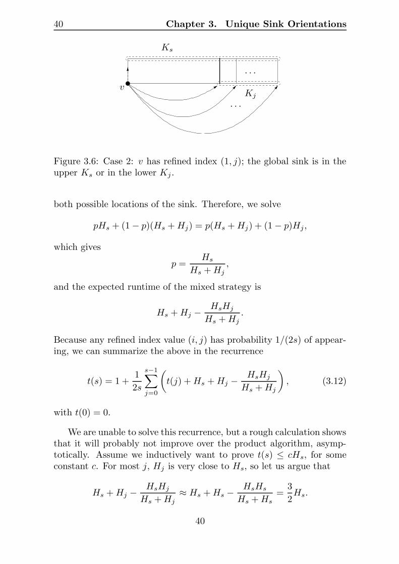
If v’s refined index is (1, j), we know that the global sink is either inthe complete graph Ks not containing v, or in the Kj spanned by theneighbors of v along its j outgoing edges, see Figure 3.6. Strategy 1 isto evaluate the sink of the Ks first, and if this didn’t turn up the globalsink, do the Kj afterwards. Strategy 2 proceeds vice versa. Taking intoaccount that Hm evaluations are necessary and sufficient to deal withKm, we arrive at the following runtimes of the two strategies.
sink is in Ks sink is in Kj
Strategy 1 Hs Hs +Hj
Strategy 2 Hs +Hj Hj
We choose a mixed strategy resulting from running Strategy 1 withprobability p and Strategy 2 with probability 1 − p. The best p isobtained when the mixed strategy has the same expected runtime for
39
40 Chapter 3. Unique Sink Orientations
PSfrag replacements
· · ·
· · ·
Kj
Ks
v
Figure 3.6: Case 2: v has refined index (1, j); the global sink is in theupper Ks or in the lower Kj .
both possible locations of the sink. Therefore, we solve
pHs + (1 − p)(Hs +Hj) = p(Hs +Hj) + (1 − p)Hj,
which gives
p =Hs
Hs +Hj,
and the expected runtime of the mixed strategy is
Hs +Hj −HsHj
Hs +Hj.
Because any refined index value (i, j) has probability 1/(2s) of appear-ing, we can summarize the above in the recurrence
t(s) = 1 +1
2s
s−1∑
j=0
(
t(j) +Hs +Hj −HsHj
Hs +Hj
)
, (3.12)
with t(0) = 0.
We are unable to solve this recurrence, but a rough calculation showsthat it will probably not improve over the product algorithm, asymp-totically. Assume we inductively want to prove t(s) ≤ cHs, for someconstant c. For most j, Hj is very close to Hs, so let us argue that
Hs +Hj −HsHj
Hs +Hj≈ Hs +Hs −
HsHs
Hs +Hs=
3
2Hs.
40

3.3. Ladders 41
In order for the inductive proof to work, we should then have
1 +1
2s
s−1∑
j=0
(
t(j) +Hs +Hj −HsHj
Hs +Hj
)
≈ 3
4Hs +
c
2s
s−1∑
j=0
Hj
≈ 3
4Hs +
c
2Hs
≤ cHs,
which gives c ≥ 3/2.
Let us do some numerical evaluations of the bounds in (3.11) and(3.12). The following table gives some values (all values have beenexactly computed first and then rounded).
s 1 2 3 13 14 50 100Product 3/2 86/40 2.65 4.670 4.7773 6.65 7.68Refined Index 3/2 89/40 2.71 4.672 4.7769 6.61 7.62
The product algorithm is still better than the refined index algorithmfor s ≤ 13, but starting from s = 14, refined index wins. The marginis not very large, though, and it is not clear whether this margin goesto infinity with s, or whether it is bounded by some constant. Exactcomputations of values become very slow for s > 100, and even whenwe do all computations in floating-point, Maple2 is slow. For s = 200,the floating-point computations almost reach their limit; we get 8.72 forproduct and 8.65 for refined index.
3.3.2 A better Algorithm for s = 3?
Here is a specific algorithm for s = 3 which seems to make sense. Asin the refined index algorithm, a random vertex is evaluated first, anddepending on its refined index, further actions are taken. Figure 3.7summarizes the algorithm.
Here are the runtimes in the various cases. As above, we apply theoptimal mixed strategy in cases (1, 1) and (1, 2). In all other cases, we
2http://www.maplesoft.com/
41
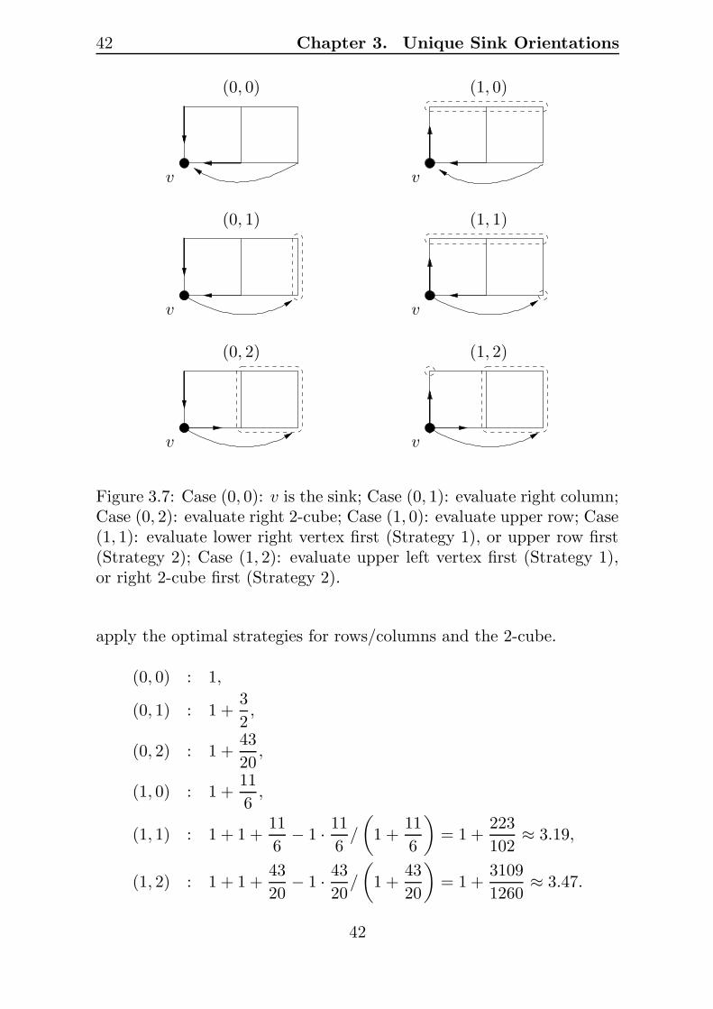
42 Chapter 3. Unique Sink Orientations
PSfrag replacements
v
v
v
v
vv
(0, 0)
(0, 1)
(0, 2)
(1, 0)
(1, 1)
(1, 2)
Figure 3.7: Case (0, 0): v is the sink; Case (0, 1): evaluate right column;Case (0, 2): evaluate right 2-cube; Case (1, 0): evaluate upper row; Case(1, 1): evaluate lower right vertex first (Strategy 1), or upper row first(Strategy 2); Case (1, 2): evaluate upper left vertex first (Strategy 1),or right 2-cube first (Strategy 2).
apply the optimal strategies for rows/columns and the 2-cube.
(0, 0) : 1,
(0, 1) : 1 +3
2,
(0, 2) : 1 +43
20,
(1, 0) : 1 +11
6,
(1, 1) : 1 + 1 +11
6− 1 · 11
6/
(
1 +11
6
)
= 1 +223
102≈ 3.19,
(1, 2) : 1 + 1 +43
20− 1 · 43
20/
(
1 +43
20
)
= 1 +3109
1260≈ 3.47.
42

3.3. Ladders 43
The average of these six values is
43207
16065≈ 2.69
and equals the expected number of vertex evaluations. Unfortunately,this number is larger than that obtained from the product algorithm,so what went wrong? It seems that in cases (0, 1), (0, 2), (1, 0), we canhardly do better: we know a subgrid containing the sink, but we haveno information about the edge orientations within the subgrid. In thissituation, the generic optimal algorithm for the subgrid should be ap-plied. In the difficult cases (1, 1) and (1, 2), it is not clear, though, thatit is best to handle the two subgrids that may contain a sink (one ofthem a vertex) separately. Apparently, it’s not. Other subdivisions aredepicted in Figure 3.8, but they are worse, as you can check. The prob-
PSfrag replacements
vv
(1, 1) (1, 2)
Figure 3.8: Worse ways of subdividing the possible sink locations intotwo subgrids.
lem is therefore to find better or even optimal strategies to deal withcases (1, 1) and (1, 2). In the following, by solving a linear program, wewill develop an optimal algorithm for the 3-ladder. But first – in orderto keep the LP as small as possible – we define isomorphisms of grids.
3.3.3 Isomorphisms on General Grid USOs
Remember that a vertex in the n-dimensional grid([N ],Π) is a set con-sisting of exactly one element out of each block Πi, i = 1, . . . , n. In thefollowing, we stick to the bit-model, where we represent such a set byits N -dimensional characteristic vector, partitioned into n blocks. Thenumber of bits of a block is the size of the corresponding grid dimension.Given a USO ψ of the grid([N ],Π), the outgoing edges of a vertex V
43
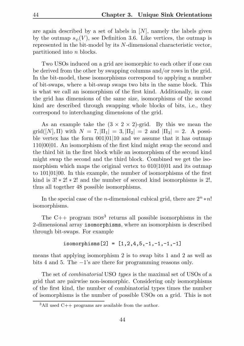
44 Chapter 3. Unique Sink Orientations
are again described by a set of labels in [N ], namely the labels givenby the outmap sψ(V ), see Definition 3.6. Like vertices, the outmap isrepresented in the bit-model by its N -dimensional characteristic vector,partitioned into n blocks.
Two USOs induced on a grid are isomorphic to each other if one canbe derived from the other by swapping columns and/or rows in the grid.In the bit-model, these isomorphisms correspond to applying a numberof bit-swaps, where a bit-swap swaps two bits in the same block. Thisis what we call an isomorphism of the first kind. Additionally, in casethe grid has dimensions of the same size, isomorphisms of the secondkind are described through swapping whole blocks of bits, i.e., theycorrespond to interchanging dimensions of the grid.
As an example take the (3 × 2 × 2)-grid. By this we mean thegrid([N ],Π) with N = 7, |Π1| = 3, |Π2| = 2 and |Π3| = 2. A possi-ble vertex has the form 001|01|10 and we assume that it has outmap110|00|01. An isomorphism of the first kind might swap the second andthe third bit in the first block while an isomorphism of the second kindmight swap the second and the third block. Combined we get the iso-morphism which maps the original vertex to 010|10|01 and its outmapto 101|01|00. In this example, the number of isomorphisms of the firstkind is 3! ∗ 2! ∗ 2! and the number of second kind isomorphisms is 2!,thus all together 48 possible isomorphisms.
In the special case of the n-dimensional cubical grid, there are 2n∗n!isomorphisms.
The C++ program isos3 returns all possible isomorphisms in the2-dimensional array isomorphisms, where an isomorphism is describedthrough bit-swaps. For example
isomorphisms[2] = [1,2,4,5,-1,-1,-1,-1]
means that applying isomorphism 2 is to swap bits 1 and 2 as well asbits 4 and 5. The −1’s are there for programming reasons only.
The set of combinatorial USO types is the maximal set of USOs of agrid that are pairwise non-isomorphic. Considering only isomorphismsof the first kind, the number of combinatorial types times the numberof isomorphisms is the number of possible USOs on a grid. This is not
3All used C++ programs are available from the author.
44

3.3. Ladders 45
PSfrag replacements
(i) (ii) (iii)
Figure 3.9: Number of combinatorial USO types of Ls.
the case with isomorphisms of the second kind (for example, regardingonly second kind isomorphisms, there are 8 combinatorial USO types ofthe 2-cube and two isomorphisms). The following table collects somevalues computed by the programs isos and lp generator (to whichwe return later). Since we’ll analyze HK orientations shortly, we alsoinclude the number of combinatorial types that are HK.
#Isos #Combs #HK-Combs #Usos
1-cube 2 1 1 22-cube 8 2 2 123-cube 48 19 17 7444-cube 384 14614 ? 5541744d-grid d! 1 1 d!(3 × 2)-grid 12 11 10 132(4 × 2)-grid 48 47 40 2256(5 × 2)-grid 240 231 192 55440(3 × 3)-grid 72 82 45 5796(3 × 2 × 2)-grid 48 2330 1322 110760
The number of combinatorial USO types for the 4-cube is due to Schurr[81]. We restrict our focus to ladders, which are (2 × s)-grids. Isomor-phisms of the second kind do not apply here (for s 6= 2).
Lemma 3.13 The number of combinatorial USO types on the s-ladder,c(s), obeys the following recurrence:
c(s) =
s∑
i=1
c(s− i) ∗ i!, c(0) = 1.
Proof. Fix the leftmost edge to go upwards and all edges in the bottom
45

46 Chapter 3. Unique Sink Orientations
row of the ladder to go from left to right. This is indicated by the thickarrow in Figure 3.9 (i). Every USO that can be achieved by completingthis partial orientation to a USO defines a distinct combinatorial type.An orientation of the vertical edges gives us a partition of the ladderinto blocks of upward and downward going edges. For example, inFigure 3.9 (ii), the first block consists of 2, the second of 3 and thethird of 3 up-/downward directed edges. Such a partition is given by itscharacterization P := (p1, p2, ..., pk), where pi is the number of verticaledges in the ith block. Given a characterization, the number of possibleUSO completions is P ! := p1! ∗ p2! ∗ . . . ∗ pk!. This can be seen throughFigure 3.9 (iii), where the forced orientations of three further edges areshown. One can see that the horizontal edges between different blockshave to be oriented to the right in order to prevent cycles or multiplesinks in subgrids. Edges connecting two vertices in the same block arethus the only ones whose orientation is not yet fixed. In block i, thereare pi! possibilities to orient the edges.
All together, the number of combinatorial USO types is∑
P P !.Arguing in terms of the formula in the lemma, we have i! possibilitiesto orient the edges in the first block of size i (note that the first blockhas size at least 1) and then c(s− i) possibilities to orient the remaining(s− i)-ladder. �
For s = 1, . . . , 6 we get 1, 3, 11, 47, 231, 1303 combinatorial USOtypes. Observe that for the 2-ladder – which is the 2-cube – we get3 combinatorial types in contrast to 2 combinatorial types in the tableabove. This is because we ignore isomorphisms of the second kind.
We are not able to give a closed form for the recurrence. Karttunenpoints out [46] that the sequence generated by the recurrence could bethe invert transform of the factorial numbers, but he has no proof. Theinvert transform is given for example in [2].
3.3.4 Optimal Strategies and Zero-Sum Games
The problem of finding an optimal strategy, w.r.t. the number of ver-tex evaluations needed to find the sink in a grid USO, can be stated asa zero-sum game between two players [29]. One player, the algorithmplayer, wants to find a probability distribution over the possible algo-
46

3.3. Ladders 47
rithms such that the number of vertex evaluations is minimized withrespect to the underlying USO played by the second player. The sec-ond player, the adversary, wants to play the USOs according to someprobability distribution maximizing the number of evaluations the al-gorithm player needs. Using results in game theory, it is possible toget the optimal strategies for both players by solving a linear program.Although this LP is in general too big to handle, the methods of Tessaro[91] allow us to drastically reduce the size of the LP by making use ofisomorphisms and thereby restricting to combinatorial USO types. Weadapted Tessaro’s program for cube USOs to work for grids.
The C++ program lp generator needs as inputs the possibleUSOs of the grid (generated with the program grid uso) and all iso-morphisms (generated with isos, see above). It outputs the LP eitherin Maple or cplex format. The latter can be processed by the cplex
solver4 or can be converted (using cplex) to MPS format which in turncan be processed by Masashi Kiyomi’s exlp solver5. While cplex isvery fast but does not compute with exact arithmetic, exlp is exact butslow (but still faster than Maple). Here is an overview of the solutionsfound:
Optimal expected number of vertex evaluationsRational value Floating value
1-cube 3/2 1.52-cube 43/20 2.153-cube 4074633/1369468 2.97534005913-cube HK 62386353/21024728 2.9672846659d-grid Hd
(3 × 2)-grid 10001/3912 2.5564928425(3 × 2)-grid HK 611/240 2.5458333333(4 × 2)-grid 28491130033/9987432048 2.8526982608(4 × 2)-grid HK 4827433/1704792 2.8316844518(3 × 3)-grid 2.9941171939(3 × 3)-grid HK 2.9654439873
The LP for the (3 × 3)-grid is already too large to be solved by exlp.It is remarkable that all grids in the table need less than 3 expectedvertex evaluations (the 1-dimensional d-grid for d ≤ 10).
4http://www.cplex.com5http://members.jcom.home.ne.jp/masashi777/exlp.html
47

48 Chapter 3. Unique Sink Orientations
Figure 3.10: The eye (left) and the bow (right).
An optimal strategy for the algorithm player is encoded in the solu-tion to the primal LP. For the 1-cube, the strategy is easy: evaluate oneof the two vertices. If it is the sink stop, else evaluate the second vertexas well. The strategy for the 2-cube is described in [89]. Not giventhere is the strategy for the adversary, which can be derived by solvingthe dual LP. Optimally, the adversary chooses an eye (see Figure 3.10)with probability 1
5 and a bow with probability 45 . The strategy for the
3-cube has first been computed by Rote (this was not published, thepaper [89] contains a “personal communication” reference). It has beenverified and analyzed in more detail in [91]. We restrict ourselves tothe optimal strategy for the 3-ladder, optimal strategies for larger gridsseem too difficult to describe.
3.3.5 The 3-Ladder
After presolving, cplex solves the sparse LP consisting of 48 rows, 179columns and 1073 nonzeros in a few milliseconds. The LP is actuallysmall enough to be solved by Maple, which yields the rational valueof 10001/3912 for the objective function (expected number of vertexevaluations) and rational values for the solution values of the variables,from which an optimal strategy can be read off. The LP is degenerate,i.e., there exists more than one solution. In fact there are infinitelymany solutions, since every convex combination of solutions is again asolution (Lemma 3.29 in [91]).
The optimal strategy found is given in form of a game tree [29] inFigures 3.11 and 3.12, where the latter figure describes the strategywhen the first vertex evaluated is the source.
Going from top to bottom in the game tree, moves of the algorithm
48

3.3
.Ladders
49
263/652
200/26363/263
171/652218/652
582/652 70/652
PSfrag replacements
Figure 3.12
Figure 3.11: An optimal strategy. See Figure 3.12 for the case where the source is evaluated first.
49

50
Chapte
r3.
Uniq
ue
Sin
kO
rienta
tions
226/652
110/226116/226 84/226 142/226
110/652316/652
Figure 3.12: The first vertex evaluated is the source.
50

3.3. Ladders 51
PSfrag replacements
0 10163
11163
22163
20163 0 91
326 0
20163
11163
47326
Figure 3.13: The 11 combinatorial USO types of the 3-ladder and theirprobabilities to be chosen by the adversary playing an optimal strategy.
player and the adversary alternate, starting with the algorithm playerchoosing a first vertex to evaluate (the bottom left vertex in the 3-ladder). Moves of the algorithm player not labeled by a probability arechosen with probability 1. Since the figures represent the point of viewof the algorithm player, moves of the adversary have no probability: thetree shows how to react to any possible USO. In the game tree of thedual LP, the roles of the players are interchanged and the adversary’soptimal strategy is visualized (not shown here). To save space, once thesink is determined, its evaluation is not given in the figure.
By our restriction to combinatorial types, the USOs given in thefigures are actually classes of isomorphic USOs, thus choosing the vertexat the bottom left in the first move is equivalent to choosing any vertex.Generally, if the probability to evaluate a vertex is p in the game tree,then p is uniformly distributed among all vertices in the same orbit (see[91]). Vertices are in the same orbit if they are indistinguishable withrespect to the partial combinatorial USO type determined so far.
An optimal strategy for the adversary is to choose a combinatorialUSO type with its corresponding probability given in Figure 3.13. Theseprobabilities can be read off a solution to the dual LP. The strategyshown is Maple’s solution. Again, there are infinitely many solutionsto the dual LP. Note that every optimal strategy of the adversary is a
51
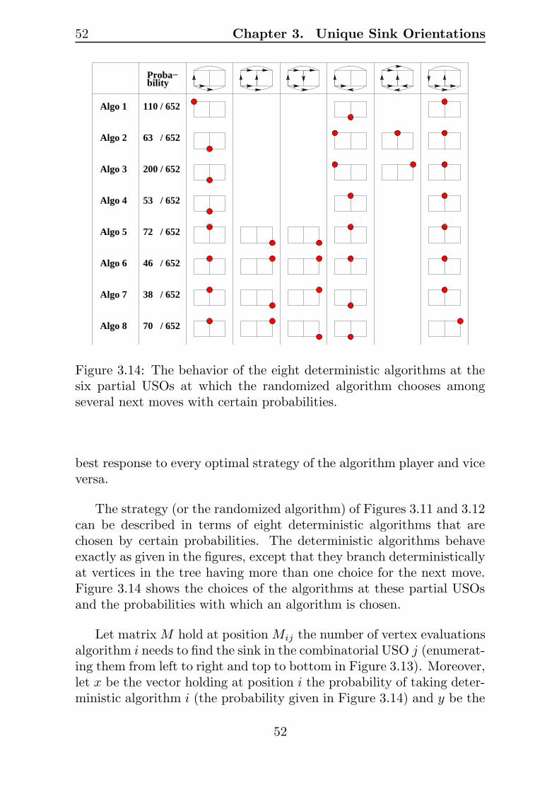
52 Chapter 3. Unique Sink Orientations
200 / 652
53 / 652
72 / 652
38 / 652
70 / 652
46 / 652
Algo 8
Algo 7
bility
63 / 652
Algo 6
Algo 5
Algo 4
Algo 3
Algo 2
Algo 1 110 / 652
Proba−
Figure 3.14: The behavior of the eight deterministic algorithms at thesix partial USOs at which the randomized algorithm chooses amongseveral next moves with certain probabilities.
best response to every optimal strategy of the algorithm player and viceversa.
The strategy (or the randomized algorithm) of Figures 3.11 and 3.12can be described in terms of eight deterministic algorithms that arechosen by certain probabilities. The deterministic algorithms behaveexactly as given in the figures, except that they branch deterministicallyat vertices in the tree having more than one choice for the next move.Figure 3.14 shows the choices of the algorithms at these partial USOsand the probabilities with which an algorithm is chosen.
Let matrix M hold at position Mij the number of vertex evaluationsalgorithm i needs to find the sink in the combinatorial USO j (enumerat-ing them from left to right and top to bottom in Figure 3.13). Moreover,let x be the vector holding at position i the probability of taking deter-ministic algorithm i (the probability given in Figure 3.14) and y be the
52

3.3. Ladders 53
vector holding at position j the probability that the adversary choosesthe combinatorial USO j (the probability given in Figure 3.13), bothvectors of appropriate size. Then one can verify that xTMy is indeed10001/3912 = 2.556, where M is the following matrix.
11/4 11/4 11/4 8/3 31/12 5/2 29/12 11/4 8/3 29/12 5/2
11/4 31/12 8/3 5/2 8/3 31/12 31/12 31/12 7/3 11/4 5/2
11/4 31/12 17/6 5/2 8/3 31/12 31/12 31/12 7/3 31/12 5/2
29/12 9/4 7/3 17/6 8/3 31/12 31/12 11/4 5/2 29/12 5/2
25/12 7/3 2 31/12 5/2 31/12 8/3 29/12 11/4 5/2 31/12
2 5/2 2 31/12 29/12 8/3 8/3 7/3 11/4 5/2 31/12
29/12 17/6 5/2 29/12 9/4 29/12 5/2 29/12 11/4 8/3 11/4
7/3 5/2 5/2 29/12 7/3 5/2 5/2 7/3 17/6 8/3 11/4
We remark that the eight deterministic algorithms actually don’t behavepurely deterministically. The first vertex to evaluate is chosen in everyalgorithm with probability 1/6 and in partial USOs where there is morethan one vertex in the orbit, the next one is chosen u.a.r. among all ofthem. For example in Figure 3.12, an algorithm that branches left afterthe very first vertex evaluation would evaluate one of the two markedvertices in the following figure with probability 1/2 each (the singlemarked vertex in Figure 3.12 is a representative for the two vertices inthe same orbit).
We see that an optimal algorithm is hard to describe already forsmall ladders. By plugging in t(3) = 10001/3912 as a base case for therecurrence (3.10)
t(s) = t(s− 1) +3
2s,
that we derived on page 38 for the product algorithm, gives
t(s) =3
2Hs −
757
3912.
53
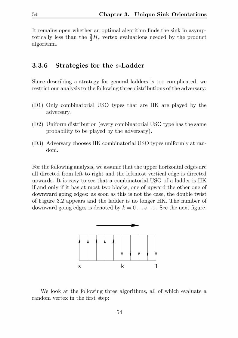
54 Chapter 3. Unique Sink Orientations
It remains open whether an optimal algorithm finds the sink in asymp-totically less than the 3
2Hs vertex evaluations needed by the productalgorithm.
3.3.6 Strategies for the s-Ladder
Since describing a strategy for general ladders is too complicated, werestrict our analysis to the following three distributions of the adversary:
(D1) Only combinatorial USO types that are HK are played by theadversary.
(D2) Uniform distribution (every combinatorial USO type has the sameprobability to be played by the adversary).
(D3) Adversary chooses HK combinatorial USO types uniformly at ran-dom.
For the following analysis, we assume that the upper horizontal edges areall directed from left to right and the leftmost vertical edge is directedupwards. It is easy to see that a combinatorial USO of a ladder is HKif and only if it has at most two blocks, one of upward the other one ofdownward going edges: as soon as this is not the case, the double twistof Figure 3.2 appears and the ladder is no longer HK. The number ofdownward going edges is denoted by k = 0 . . . s−1. See the next figure.
s k 1
We look at the following three algorithms, all of which evaluate arandom vertex in the first step:
54

3.3. Ladders 55
(A1) If the vertical edge of the evaluated vertex is outgoing, follow itand evaluate the corresponding edge-neighbor. If it is incoming,evaluate a random neighbor reachable through outgoing horizontaledges. Repeat this strategy.
(A2) If the vertical edge of the evaluated vertex is outgoing, jump toa vertex antipodal in the 2-cubical face spanned by the verticaledge and a random outgoing horizontal edge (if there is no outgo-ing horizontal edge, just follow the vertical edge). If the verticaledge is incoming, evaluate a random neighbor reachable throughoutgoing horizontal edges. Repeat this strategy.
(A3) Proceed as in (A2). If there is more than one possible vertex tobe evaluated next, choose randomly one that has fewest incomingedges evaluated so far. Repeat this strategy.
Here are some results.
(A1) (A2) (A3)(D1) Hs + 3/2 − 1/s ? ?(D2) ? ? Optimal for s ≤ 4(D3) ≤ Hs + 3/2 − 1/s ≤ Hs + 3/2 − 1/s Optimal for s ≤ 4
The expected number of vertex evaluations (runtime) of (A1) on HKladders depends only on the (adversary’s) choice of k. For k = 0 it isHs + 1/2. For k > 0 we distinguish between start vertices in one of thefour areas given in the following figure. If the first vertex evaluated is
s k 1
the one connected to the jth step in the upper left area (j > k), then
55

56 Chapter 3. Unique Sink Orientations
the expected number of vertex evaluations is given by the recurrence
t(j) = 1 +1
j − 1
j−1∑
i=k+1
t(i) +1
j − 1
k∑
i=1
(1 +Hk).
So (j−1) · t(j)− (j−2) · t(j−1) = 1+ t(j−1) holds for j ≥ k+2 whichimplies t(j) = 1
j−1 + t(j − 1). This results in t(j) = Hj−1 + 2 for j > k.
Given this, the runtime for start vertices in the other areas are easyto derive. Since the starting vertex is picked uniformly at random, theoverall runtime is
T (s) =1
2s(
upper left︷ ︸︸ ︷s∑
i=k+1
t(i) +
s∑
i=k+1
(1 + t(i))
︸ ︷︷ ︸
lower left
+
upper right︷ ︸︸ ︷
k∑
i=1
(1 +Hk)+
k∑
i=1
Hk
︸ ︷︷ ︸
lower right
)
=1
s
s∑
i=k+1
t(i) +k
sHk +
1
2
=1
s
s∑
i=k+1
(Hi−1 + 2) +k
sHk +
1
2
=1
s(sHs−1 − kHk − (s− 1) + k) +
k
sHk +
2(s− k)
s+
1
2
= Hs−1 +1 − k
s+
3
2
= Hs −k
s+
3
2,
where we use that∑bi=aHi = (b+ 1)Hb − aHa − b+ a. This is largest
for k = 1 which gives us the worst case runtime of Hs + 3/2 − 1/s onany HK ladder.
A lower bound for the runtime on a HK ladder is derived as follows.Let the adversary choose the distribution described by the followingconstruction: choose an orientation of the 1-dimensional s-grid (whichis the complete graph on s vertices) uniformly at random among all pos-sible orientations. Let the upper and lower part of the s-ladder be thisorientation and orient all vertical edges upwards, except the one formingthe step connecting the two sinks in the s-grids. This edge is directed
56

3.3. Ladders 57
upwards or downwards with probability 1/2. The resulting orientationis a HK ladder USO (k is 0 or 1). An optimal deterministic algorithmfinds the sink by evaluating either the lower or upper s-grid first andthen, if necessary (with probability 1/2), jumping to the other side forone last vertex evaluation. This results in an optimum of Hs + 1/2vertex evaluations (see also the discussion on page 37). By using Yao’sPrinciple [96] again, this is a lower bound for an optimal randomizedalgorithm finding the sink in a HK s-ladder. Our worst case runtime ofHs + 3/2− 1/s for HK ladders is therefore close to optimum. However,it is not optimal, which we can easily check by comparing to the valuesgiven in the table on page 47.
For general (not HK) ladders, the distribution where the adversaryorients all horizontal edges from left to right and all vertical edges withprobability 1/2 downwards or upwards, yields a runtime of Hs · 3/2 for(A1). So (A1) is not better than the product algorithm in general.
Algorithm (A2) is harder to analyze, since its runtime depends onthe adversary’s distribution (not only on k). If the HK ladders arechosen u.a.r., then its runtime can be computed (but the formula isquite messy) and computer experiments suggest that (A2) performsslightly better than (A1) on HK ladders chosen u.a.r.
By solving a linear program as we did it for 3-ladders, we computedthe optimal strategy for 4-ladders when the adversary chooses the uni-form distribution, once over all ladders and once only over HK ladders.It is interesting that in both cases, (A3) is an optimal algorithm to findthe sink in s-ladders with s ≤ 4. We don’t know whether this remainstrue for s > 4.
57

58 Chapter 3. Unique Sink Orientations
58

Chapter 4
Violator Spaces
Sharir and Welzl introduced an abstract framework for optimizationproblems, called LP-type problems or also generalized linear program-ming problems [84], which proved useful in algorithm design. Here wepresent the new framework of violator spaces, introduced by Matousekand Skovron in [85]. Violator spaces form, as we believe, a simpler andmore natural framework and they constitute a proper generalization ofLP-type problems. We show that grid USOs fit into this frameworkand that Clarkson’s randomized algorithms for low-dimensional linearprogramming work in the context of violator spaces. Via the reductionfrom PGLCP to grid USO (Section 3.1), we obtain the fastest knownalgorithm for the PGLCP with a constant number of blocks.
4.1 LP-Type Problems
An (abstract) LP-type problem is given by a finite set H of constraintsand a value w(G) for every subset G ⊆ H . The values can be realnumbers or, for technical convenience, elements of any other linearlyordered set. Intuitively, w(G) is the minimum value of a solution thatsatisfies all constraints in G. The assignment G 7→ w(G) has to obeythe axioms in the following definition.
59

60 Chapter 4. Violator Spaces
Definition 4.1 An abstract LP-type problem is a quadruple
(H,w,W,≤),
where H is a finite set, W is a set linearly ordered by ≤, and w: 2H →Wis a mapping satisfying the following two conditions for all F ⊆ G ⊆ H:
Monotonicity: w(F ) ≤ w(G), andLocality: if w(F ) = w(G) and w(G) < w(G ∪ {h})
for h ∈ H, then w(F ) < w(F ∪ {h}) holds.
As our running example, we will use the smallest enclosing ball prob-lem, where H is a finite point set in R
d and w(G) is the radius of thesmallest ball that encloses all points of G. In this case monotonicity isobvious, while verifying locality requires the nontrivial but well-knowngeometric result that the smallest enclosing ball is unique for every set.
It seems that the order ≤ of subsets is crucial; after all, LP-typeproblems model optimization problems, and indeed, the subexponen-tial algorithm for linear programming and other LP-type problems [57]heavily relies on such an order.
A somewhat deeper look reveals that we often only care whethertwo subsets have the same value, but not how they compare under theorder ≤. The following definition is taken from [84]:
Definition 4.2 Consider an abstract LP-type problem (H,w,W,≤). Wesay that B ⊆ H is a basis if for all proper subsets F ⊂ B we havew(F ) 6= w(B). For G ⊆ H, a basis of G is an inclusion-minimal subsetB of G with w(B) = w(G).
We observe that a minimal subset B ⊆ G with w(B) = w(G) isindeed a basis.
Solving an abstract LP-type problem (H,w,W,≤) means to find abasis of H . In the smallest enclosing ball problem, a basis of H is aminimal set B of points such that the smallest enclosing ball of B hasthe same radius (and is in fact the same) as the smallest enclosing ballof H , w(B) = w(H).
In defining bases, and in saying what it means to solve an LP-typeproblem, we therefore do not need the order ≤. This is formalized by the
60

4.1. LP-Type Problems 61
new framework of violator spaces, defined in Section 4.2. Intuitively, aviolator space is an LP-type problem without order. This generalizationof LP-type problems is proper, and we can exactly characterize theviolator spaces that “are” LP-type problems [31, 30].
Probably the most surprising insight is that Clarkson’s algorithms[11] work for violator spaces of fixed dimension, leading to an expectedlinear-time algorithm for “solving” the violator space. This is shown inSection 4.3. Clarkson’s algorithms were originally developed for linearprograms with small dimension. They can be generalized for LP-typeproblems [35, 9]. The fact that the scheme also works for violator spacesmay come as a surprise since the structure of violator spaces is notacyclic in general (in contrast to LP-type problems). Actually, it turnsout that problems effectively solvable by Clarkson’s algorithms are in awell-defined sense exactly the violator spaces [86]; see Property 4.15 fora precise formulation.
In Section 4.4 we show that any grid USO gives rise to a violatorspace, but not to an LP-type problem in general. The sink of a grid USOcan thus be found by solving the violator space, for example with Clark-son’s algorithms. A concrete new result is obtained by applying this tothe PGLCP. Since any PGLCP gives rise to a unique sink orientation(Theorem 3.5), we may use violator spaces and Clarkson’s algorithms tosolve the problem in expected linear time in the (polynomially solvable)case of a fixed number of blocks. This is optimal and beats all previousalgorithms.
A unique sink orientation can be cyclic and we show that a cyclicorientation gives rise to a cyclic violator space and does therefore notfit into the LP-type framework. Unique sink orientations are thus non-trivial examples of possibly cyclic violator spaces. We are confidentthat more applications of violator spaces that are not subsumed by theLP-type framework will be discovered in the future.
61

62 Chapter 4. Violator Spaces
4.2 The Violator Space Framework
Let (H,w,W,≤) be an abstract LP-type problem. It is natural to definethat a constraint h ∈ H violates a set G ⊆ H of constraints if
w(G ∪ {h}) > w(G).
For example, in the smallest enclosing ball problem, a point h violates aset G if it lies outside of the smallest ball enclosing G (which is unique).
Definition 4.3 The violator mapping of (H,w,W,≤) is defined byV(G) = {h ∈ H :w(G ∪ {h}) > w(G)}. Thus, V(G) is the set of allconstraints violating G.
It is shown in [31, 30] that the knowledge of V(G) for all G ⊆ His sufficient to describe the “structure” of an LP-type problem. Thatis, while we cannot reconstruct W , ≤, and w from this knowledge,it is natural to regard two LP-type problems with the same mappingV: 2H → 2H as isomorphic. Indeed, the algorithmic primitives neededfor implementing the Sharir-Welzl algorithm and the other algorithmsfor LP-type problems mentioned above can be phrased in terms of test-ing violation (does h ∈ V(G) hold for a certain set G ⊆ H?), and theynever deal explicitly with the values of w.
We now introduce the notion of violator space:
Definition 4.4 A violator space is a pair (H,V), where H is a finiteset and V is a mapping 2H → 2H such that
Consistency: G ∩ V(G) = ∅ holds for all G ⊆ H, andLocality: for all F ⊆ G ⊆ H, if G ∩ V(F ) = ∅,
then V(G) = V(F ).
A basis of a violator space is defined in analogy to a basis of anLP-type problem.
Definition 4.5 Consider a violator space (H,V). We say that B ⊆ His a basis if for all proper subsets F ⊂ B we have B ∩ V(F ) 6= ∅. ForG ⊆ H, a basis of G is a minimal subset B of G with V(B) = V(G).
62

4.2. The Violator Space Framework 63
Observe that a minimal subset B ⊆ G with V(B) = V(G) is indeeda basis: Assume for contradiction that there is a set F ⊂ B such thatB ∩ V(F ) = ∅. Locality then yields V(B) = V(F ) = V(G), whichcontradicts minimality of B.
In [31, 30] it is shown that an abstract LP-type problem (H,w,W,≤)is, in a natural sense, isomorphic to an acyclic violator space (H,V) withV being the violator mapping. We now prepare to define the notion ofan acyclic violator space. The example of a cyclic violator space atthe end of this section then shows that violator spaces are a propergeneralization of LP-type problems.
We fix a violator space (H,V). The set of all bases in (H,V) will bedenoted by B.
Definition 4.6 B,C ∈ B are equivalent, B ∼ C, if V(B) = V(C).
Clearly, the relation ∼ defined on B is an equivalence relation. Theequivalence class containing a basis B will be denoted by [B]. Thefollowing definition of an ordering of the equivalence classes is neededfor the notion of acyclicity in violator spaces.
Definition 4.7 For F,G ⊆ H in a violator space (H,V), we say thatF ≤0 G (F is locally smaller than G) if F ∩V(G) = ∅. For equivalenceclasses [B], [C] ∈ B/∼, we say that [B] ≤0 [C] if there exist B′ ∈ [B]and C ′ ∈ [C] such that B′ ≤0 C
′.
The intuition of the locally-smaller notion comes from LP-type prob-lems: if no element of F violates G, then G ∪ F has the same value asG (this is formally proved in [31, 30]), and monotonicity yields thatvalue-wise, F is smaller than or equal to G.
Note that in the definition of [B] ≤0 [C] we do not require B′ ≤0 C′
to hold for every B′ and C ′. It may happen that B′ 6≤0 C′ for some
bases B′ and C ′. However, C ′ ≤0 B′ cannot hold, as one can check.
We are now ready to define acyclic violator spaces.
63

64 Chapter 4. Violator Spaces
�
�
�
Figure 4.1: A cyclic violator space.
Definition 4.8 Let the relation ≤1 on the equivalence classes be thetransitive closure of ≤0. The relation ≤1 is clearly reflexive and tran-sitive. If it is antisymmetric, we say that the violator space is acyclic,and we define the relation ≤ as an arbitrary linear extension of ≤1.
To show that acyclicity need not always hold, we conclude this Sec-tion with an example of a cyclic violator space. We begin with anintuitive geometric description, see Figure 4.1, where we consider a tri-angle without the center point. We say that one point of the triangle is“locally smaller” than another if it is farther clockwise with respect tothe center. The constraints in our violator space are the three halfplanesf, g, h.
The locally smallest point within each halfplane is marked, and ahalfplane violates a set of halfplanes if it does not contain the locallysmallest point in their intersection.
Now we specify the corresponding violator space formally. We haveH = {f, g, h}, and V is given by the following table:
G ∅ f g h f, g f, h g, h f, g, hV(G) f, g, h h f g h g f ∅
This (H,V) is really a violator space, since we can easily check bothconsistency and locality. The bases are ∅, one-element sets, and H . We
64

4.3. Clarkson’s Algorithms 65
have {f} ≤0 {h} ≤0 {g} ≤0 {f}, but no two of the one-element basesare equivalent; i.e., ≤1 is not antisymmetric.
4.3 Clarkson’s Algorithms
We show that Clarkson’s randomized reduction scheme, originally de-veloped for linear programs with many constraints and few variables,actually works for general (possibly cyclic) violator spaces. The twoalgorithms of Clarkson involved in the reduction have been analyzedfor LP and LP-type problems before [11, 35, 9]. The analysis we givebelow is almost identical on the abstract level. Our new contribution isthat the combinatorial properties underlying Clarkson’s algorithms alsohold for violator spaces.
We start off by deriving these combinatorial properties. The analysisof Clarkson’s reduction scheme is included for completeness. We notethat the Sharir-Welzl algorithm is also applicable for violator spaces ina straightforward way. However, the most obvious translation of thisalgorithm to the setting of violator spaces is not even guaranteed tofinish, since for a general violator space it may run in a cycle and thesubexponential analysis thus breaks down.
4.3.1 Violator Spaces revisited
We recall that an abstract LP-type problem is defined by a quadruple(H,w,W,≤). In this subsection we will view a violator space as an “LP-type problem without the order ≤”, i.e., we will only care whether twosubsets F and G, F ⊆ G ⊆ H , have the same value, but not how theycompare under the order ≤. It turns out that the order is irrelevant forClarkson’s algorithms.
Even without an order, we can talk about monotonicity in violatorspaces:
Lemma 4.9 Any violator space (H,V) satisfies monotonicity definedas follows:
65

66 Chapter 4. Violator Spaces
Monotonicity: V(F ) = V(G) implies V(F ) = V(E) = V(G)for all sets F ⊆ E ⊆ G ⊆ H.
Proof. Assume V(E) 6= V(F ),V(G). Then locality yields ∅ 6= E ∩V(F ) = E ∩ V(G) which contradicts consistency. �
Recall Definition 4.5: a basis is a set B satisfying B ∩ V(F ) 6= ∅ forall proper subsets F of B. A basis of G is an inclusion-minimal subset ofG with the same violators. This can be used to prove Observation 4.10,well-known to hold for LP-type problems [35].
Observation 4.10 Let (H,V) be a violator space. For G ⊆ H and allh ∈ H, we have
(i) V(G) 6= V(G ∪ {h}) if and only if h ∈ V(G), and
(ii) V(G) 6= V(G \ {h}) if and only if h is contained in every basis ofG.
An element h such that (ii) holds is called extreme in G.
Proof. (i) If h /∈ V(G), we get V(G) = V(G ∪ {h}) by locality. Ifh ∈ V(G), then V(G) 6= V(G ∪ {h}) is a consequence of consistencyapplied to G ∪ {h}. (ii) If V(G) = V(G \ {h}), there is a basis B ofG \ {h}, and this basis, which does not contain h, is also a basis ofG. Conversely, if there is some basis B of G not containing h, thenV(G) = V(G \ {h}) follows from monotonicity (Lemma 4.9). �
We are particularly interested in violator spaces with small bases.
Definition 4.11 Let (H,V) be a violator space. The size of a largestbasis is called the combinatorial dimension δ = δ(H,V) of (H,V).
Observation 4.10 implies that in a violator space of combinatorialdimension δ, every set has at most δ extreme elements. This in turnyields a bound for the expected number of violators of a random subsetof constraints:
66

4.3. Clarkson’s Algorithms 67
Lemma 4.12 Let (H,V) be a violator space of combinatorial dimensionδ and W ⊆ H some fixed set. Let vr be the expected number of violatorsof the set W ∪R, where R ⊆ H \W is a random subset of size r < N =|H |. Then
vr ≤ δN − r
r + 1.
The lemma can be proved using the Sampling Lemma of [36]. We givean independent proof here.
Proof. By definition of vr and Observation 4.10
(|H \W |r
)
vr =∑
R⊆H\W|R|=r
∑
h∈(H\W )\R
[h violates W ∪R]
=∑
R⊆H\W|R|=r
∑
h∈(H\W )\R
[h is extreme in W ∪ (R ∪ {h})].
Here [A] is the indicator variable for the event A that has value 1 if Aholds and 0 otherwise.
Substituting Q for R ∪ {h} and using the fact that any set has atmost δ extreme elements, we can rewrite this as
(|H \W |r
)
vr =∑
Q⊆H\W|Q|=r+1
∑
h∈Q
[h is extreme in W ∪Q]
≤∑
Q⊆H\W|Q|=r+1
δ =
(|H \W |r + 1
)
δ.
This yields vr ≤ δ(|H \W | − r)/(r + 1), and the lemma follows. �
4.3.2 The Trivial Algorithm
Given a violator space (H,V) of combinatorial dimension δ, the goal isto find a basis of H . For this, we assume availability of the followingprimitive, which we use for sets G of size at most δ.
67

68 Chapter 4. Violator Spaces
Primitive 4.13 Given G ⊆ H and h ∈ H \ G, decide whether h ∈V(G).
Given this primitive, a basis of H can be found in a brute-forcemanner by going through all sets of size at most δ, testing each of themfor being a basis of H . More generally, B ⊆ G is a basis of G if andonly if
h ∈ V(B \ {h}), for all h ∈ B, andh /∈ V(B), for all h ∈ G \B.
Consequently, the number of times the primitive needs to be invoked inorder to find a basis of H (|H | = N) is at most
Nδ∑
i=0
(N
i
)
= O(N δ+1).
The next two subsections show that this can be substantially improved.
4.3.3 Clarkson’s First Algorithm
Fix a violator space (H,V) of combinatorial dimension δ, implicitlyspecified through Primitive 4.13. Clarkson’s first algorithm calls Clark-son’s second algorithm (Basis2) as a subroutine. Given G ⊆ H , bothalgorithms compute a basis B of G.
Basis1(G):(* computes a basis B of G *)IF |G| ≤ 9δ2 THEN
RETURN Basis2(G)ELSE
r := bδ√
|G|cW := ∅REPEAT
choose R to be a random r-element subset of G \WC := Basis2(W ∪R)V := {h ∈ G \ C:h ∈ V(C)}IF |V| ≤ 2
√
|G| THENW := W ∪ V
68
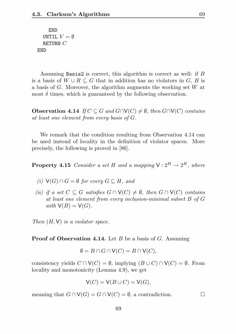
4.3. Clarkson’s Algorithms 69
END
UNTIL V = ∅RETURN C
END
Assuming Basis2 is correct, this algorithm is correct as well: if Bis a basis of W ∪ R ⊆ G that in addition has no violators in G, B isa basis of G. Moreover, the algorithm augments the working set W atmost δ times, which is guaranteed by the following observation.
Observation 4.14 If C ⊆ G and G∩V(C) 6= ∅, then G∩V(C) containsat least one element from every basis of G.
We remark that the condition resulting from Observation 4.14 canbe used instead of locality in the definition of violator spaces. Moreprecisely, the following is proved in [86].
Property 4.15 Consider a set H and a mapping V : 2H → 2H , where
(i) V(G) ∩G = ∅ for every G ⊆ H, and
(ii) if a set C ⊆ G satisfies G ∩ V(C) 6= ∅, then G ∩ V(C) containsat least one element from every inclusion-minimal subset B of Gwith V(B) = V(G).
Then (H,V) is a violator space.
Proof of Observation 4.14. Let B be a basis of G. Assuming
∅ = B ∩G ∩ V(C) = B ∩ V(C),
consistency yields C ∩ V(C) = ∅, implying (B ∪ C) ∩ V(C) = ∅. Fromlocality and monotonicity (Lemma 4.9), we get
V(C) = V(B ∪ C) = V(G),
meaning that G ∩ V(G) = G ∩ V(C) = ∅, a contradiction. �
69
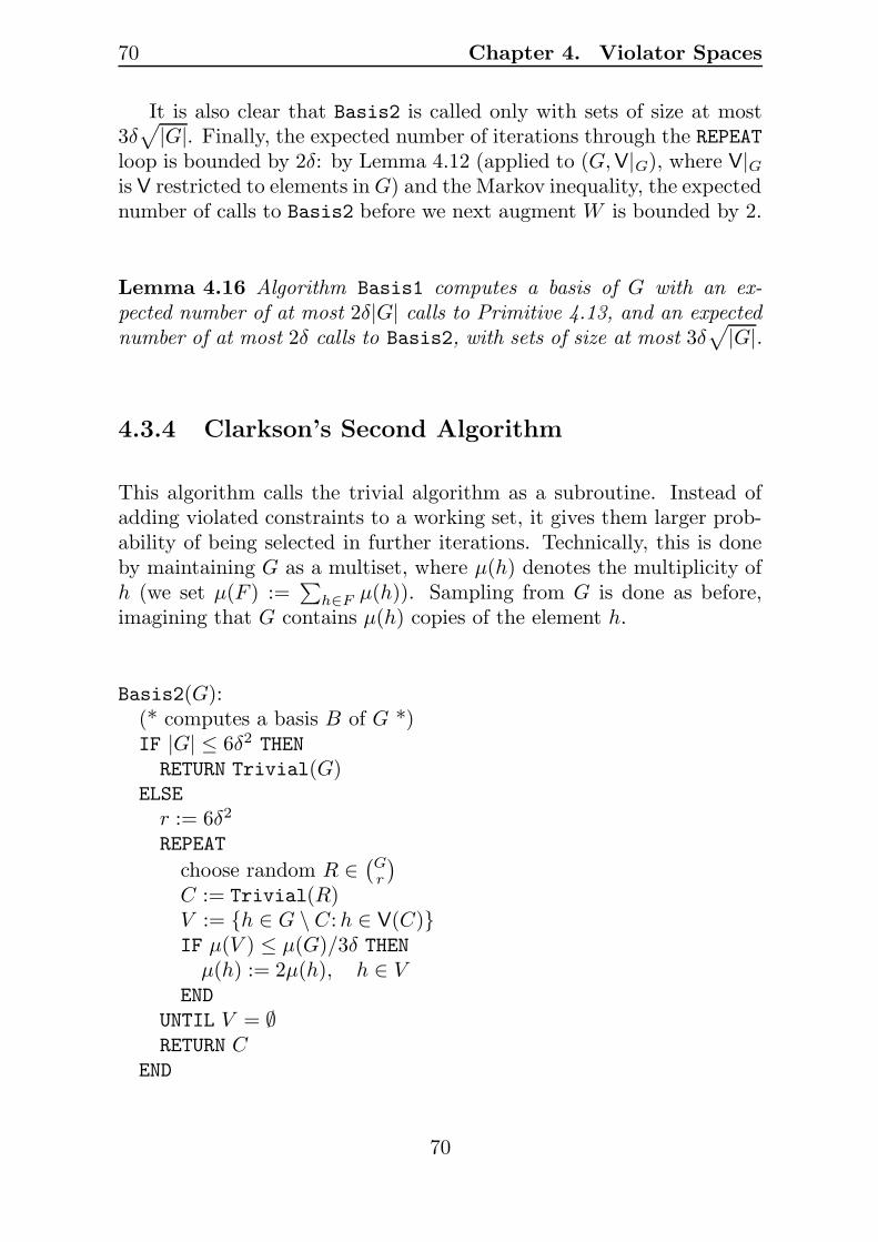
70 Chapter 4. Violator Spaces
It is also clear that Basis2 is called only with sets of size at most3δ√
|G|. Finally, the expected number of iterations through the REPEATloop is bounded by 2δ: by Lemma 4.12 (applied to (G,V|G), where V|Gis V restricted to elements inG) and the Markov inequality, the expectednumber of calls to Basis2 before we next augment W is bounded by 2.
Lemma 4.16 Algorithm Basis1 computes a basis of G with an ex-pected number of at most 2δ|G| calls to Primitive 4.13, and an expectednumber of at most 2δ calls to Basis2, with sets of size at most 3δ
√
|G|.
4.3.4 Clarkson’s Second Algorithm
This algorithm calls the trivial algorithm as a subroutine. Instead ofadding violated constraints to a working set, it gives them larger prob-ability of being selected in further iterations. Technically, this is doneby maintaining G as a multiset, where µ(h) denotes the multiplicity ofh (we set µ(F ) :=
∑
h∈F µ(h)). Sampling from G is done as before,imagining that G contains µ(h) copies of the element h.
Basis2(G):(* computes a basis B of G *)IF |G| ≤ 6δ2 THEN
RETURN Trivial(G)ELSE
r := 6δ2
REPEAT
choose random R ∈(Gr
)
C := Trivial(R)V := {h ∈ G \ C:h ∈ V(C)}IF µ(V ) ≤ µ(G)/3δ THENµ(h) := 2µ(h), h ∈ V
END
UNTIL V = ∅RETURN C
END
70

4.3. Clarkson’s Algorithms 71
Here Trivial(G) refers to calling the brute-force search algorithmdescribed below Primitive 4.13.
Invoking Lemma 4.12 again (which also applies to multisets as weuse them), we see that the expected number of calls to Trivial beforewe next reweight elements (a successful iteration), is bounded by 2. Itremains to bound the number of successful iterations.
Lemma 4.17 Let k be a positive integer. After kδ successful iterations,we have
2k ≤ µ(B) ≤ |G|ek/3,for every basis B of G. In particular, k < 3 ln |G|.
Proof. Every successful iteration multiplies the total weight of ele-ments in G by at most (1 + 1/3δ), which gives the upper bound (notonly for µ(B) but actually for µ(G)). For the lower bound, we useObservation 4.14 again to argue that each successful iteration doublesthe weight of some element in B, meaning that after kδ iterations, oneelement has been doubled at least k times. Because the lower boundexceeds the upper bound for k ≥ 3 ln |G|, the bound on k follows. �
Summarizing, we get the following lemma.
Lemma 4.18 Algorithm Basis2 computes a basis of G with an ex-pected number of at most 6δ|G| ln |G| calls to Primitive 4.13, and ex-pected number of at most 6δ ln |G| calls to Trivial, with sets of size6δ2.
4.3.5 Combining the Algorithms
Theorem 4.19 Using a combination of the above two algorithms, a ba-sis of H in a violator space (H,V) can be found by calling Primitive 4.13expected
O(
δN + δO(δ))
many times.
71

72 Chapter 4. Violator Spaces
Proof. Using the above bound for the trivial algorithm, Basis2 can beimplemented to require an expected number of at most
O(
δ log |G|(|G|+ δO(δ)))
calls to the primitive. Applying this as a subroutine in Basis1(H) with|H | = N , |G| is bounded by 3δ
√N , and we get an overall expected
complexity of
O(
δN + δ2(logN(δ√N + δO(δ)))
)
in terms of the number of calls to Primitive 4.13. The terms δ2 logN δ√N
and δ2 logN δO(δ) are asymptotically dominated by either δN or δO(δ),and we get the simplified bound of O
(δN + δO(δ)
). �
4.4 Grid USO as Models for Violator Spaces
We show in this section that the problem of finding the sink in a USOof the n-dimensional grid([N ],Π) can be reduced to the problem offinding the (unique) basis of a violator space (H,V) with H = [N ] andcombinatorial dimension n. For a better understanding, we recommendto refresh the definitions of grid, subgrid, USO and outmap, given inSection 3.1 starting on page 30.
A vertex J in the grid graph is a subset of [N ] consisting of oneelement out of each block Πi. There is an edge between two vertices Jand J ′ if and only if J and J ′ differ in exactly one element. In orderto reduce a grid USO ψ, we need the outmap sψ(J) of a vertex J . It isimportant that a sink w.r.t. ψ has empty outmap value.
Let us fix a USO ψ of the n-dimensional grid graph G = (V , E).Given a Π-valid subset G ⊆ [N ] (a subset consisting of at least oneelement out of each block Πi), we define sink(G) ∈ V to be the uniquesink vertex in the subgrid(G,Π). For a subset G that is not Π-valid, let
G :=⋃
i:G∩Πi=∅
Πi.
Thus G is the set of elements occurring in blocks of Π disjoint from G.
72

4.4. Grid USO as Models for Violator Spaces 73
Definition 4.20 For G ⊆ [N ], define
V(G) =
{sψ(sink(G)), if G is Π-validG, if G is not Π-valid.
Theorem 4.21 The pair ([N ],V) from Definition 4.20 is a violatorspace of combinatorial dimension n. Moreover, for all Π-valid G ⊆ [N ],the unique sink of the subgrid(G,Π) corresponds to the unique basis ofG in ([N ],V).
Proof. For every G ⊆ [N ], consistency holds by definition of sink(G),sψ(J) and G. In order to prove locality for F ⊆ G ⊆ [N ], we look atthree different cases. To shortcut notation, we abbreviate subgrid(F,Π)by G(F ) for any F ⊆ [N ].
G is not Π-valid. Then, F ⊆ G is not Π-valid either. The condition∅ = G ∩ V(F ) = G ∩ F means that F is disjoint from the same blocksas G. This implies G = F , hence V(G) = V(F ).
G and F are both Π-valid. Then G(F ) is a nonempty subgrid ofG(G), and G ∩ V(F ) = ∅ means that the sink of G(F ) has no outgoingedges into G(G). Thus the unique sink of G(F ) is also a sink of G(G)and therefore the unique one. This means that sink(G) = sink(F ), fromwhich V(G) = V(F ) follows.
G is Π-valid, F is not Π-valid. Then the condition G ∩ V(F ) = ∅can never be satisfied since V(F ) = F contains at least one full blockΠi, and G ∩ Πi 6= ∅.
Next we prove that a largest basis in ([N ],V) has at most n elements.For this, let G ⊆ [N ] be a set of size larger than n. If G is Π-valid, wehave
V(G) := sψ(sink(G)) = sψ(sink(sink(G))) =: V(sink(G)),
since J = sink(J) for any vertex J . This means that G has a subset ofsize n with the same violators, so G is not a basis.
73

74 Chapter 4. Violator Spaces
If G is not Π-valid, we consider some subset B that contains exactlyone element from every block intersected by G. By definition, we haveG = B and V(G) = V(B). Since B has less than n elements, G cannotbe a basis in this case, either.
It remains to prove that for G being Π-valid, the vertex sink(G) isthe unique basis of G in ([N ],V). We have already shown that V(G) =V(sink(G)) must hold in this case. Moreover, V(sink(G)) contains nofull block Πi. On the other hand, any proper subset F of sink(G) is notΠ-valid, so its violator set does contain at least one full block. It followsthat V (F ) 6= V (sink(G)), so sink(G) is a basis of G. The argumentis complete when we can prove that no other vertex J ⊆ G is a basisof G. Indeed, such a vertex J is not a sink in G(G), meaning thatG ∩ V(J) 6= ∅. This implies V(J) 6= V(G). �
Note that the global sink of the grid USO corresponds to the uniquen-element (and Π-valid) set B with V(B) = ∅. This is exactly the setoutput by the call Basis1([N ]) of Clarkson’s algorithms, when we applyit to the violator space constructed in Definition 4.20.
Primitive 4.13 corresponds to one edge evaluation in the USO set-ting. With Theorem 4.19 we then get the following result:
Theorem 4.22 The sink in a USO of the n-dimensional grid([N ],Π)can be found by evaluating expected O
(nN + nO(n)
)edges.
For small n, the running time given in the theorem is faster than theone from the product algorithm [33, 32] which needs expected O(n!N +HnN ) edge evaluations, where HN , as used earlier, is the N -th harmonic
number. Via the reduction from PGLCP to grid USO (Section 3.1) thisyields the fastest known algorithm for PGLCP with fixed number ofblocks.
The PGLCP has in general a cyclic structure and therefore givesrise to a cyclic USO. The following lemma shows that a violator spaceobtained from a cyclic USO is cyclic as well, proving that grid USO (andPGLCP) can not be reduced to LP-type problems in general (since LP-type problems are equivalent to acyclic violator spaces [31, 30]).
Lemma 4.23 The violator space arising from a cyclic grid USO via
74

4.4. Grid USO as Models for Violator Spaces 75
Definition 4.20 is cyclic.
Proof. Remember that given a grid vertex J and j ∈ [N ]\J , JBj is theunique vertex J ′ ⊆ J ∪ {j} that is different from J . J ′ is the neighborof J in direction j. Assume that the edge {J, J ′} is directed from vertexJ ′ to vertex J in the grid USO ψ. We want to show that J ′ is locallysmaller than J , meaning that J ′ ∩ V(J) = ∅ (Definition 4.7). This isindeed true, since by consistency, the only element that could possiblybe in the intersection of J ′ and V(J) is j. But j ∈ V(J) would implythat j ∈ sψ(J), meaning that J has an outgoing edge into direction j,a contradiction to the assumption that the edge is directed from J ′ toJ .
We have shown above that every vertex J is a basis in the violatorspace. From the fact that the outmap function sψ is an injection [33, 32],it follows that no two vertices in the grid belong to the same equivalenceclass in the violator space. The result that an edge directed from J ′ to Jimplies that J ′ is locally smaller than J , means that a cycle in the gridUSO immediately implies a cycle in the violator space, see Definition 4.8.�
It is interesting that there are no cycles in a 2-dimensional grid USO[33, 32]. Whether the same is true for nondegenerate (no two bases havethe same violators) violator spaces of combinatorial dimension 2 is anopen question, see also [86].
75

76 Chapter 4. Violator Spaces
76

Part II: Specializations
In this second part of the thesis, we present two specializations of thePGLCP. The first is achieved by restricting to a subclass of P-matricescalled hidden K-matrices in Chapter 5. The GLCP with a hidden K-matrix has been proved to be solvable in polynomial time. Using theconcept of Π-compatible LPs defined in Section 2.2, we give an alterna-tive proof for this fact and strengthen the statement by showing that thearising grid USO is LP-induced and therefore acyclic. Further, a char-acterization for vertical block matrices that are not hidden K is derived.Towards the end of the chapter, we introduce a nontrivial and large sub-class of matrices that are not hidden K and show that 3-dimensionalP-matrices in this class give rise to a cyclic USO in general.
The second specialization is actually an application. We show thatsimple stochastic games (SSG) can be reduced to the PGLCP. It isopen to characterize the P-matrices we get from the games, but we givearguments indicating that not all P-matrices are SSG-induced (that’swhy we speak of a specialization). At the end of the thesis, we giveexamples of SSGs, showing that the resulting matrix in the PGLCP isneither (transpose) hidden K nor well-conditioned in general.
77

78

Chapter 5
Hidden K-Matrices
We focus on the class of hidden K-matrices which also appear under thename hidden Minkowski matrices or mime matrices (see [93]). HiddenK-matrices form a proper subclass of P-matrices. The importance of thehidden K-matrix GLCP comes from the fact that the solution can becomputed by a linear program. In order to show how this LP looks like,we need some definitions of matrix classes first, given in Section 5.1.
We then reprove that the hidden K GLCP can be solved by LP andconcurrently show that the grid USO arising from a hidden K-matrixGLCP is LP-induced and therefore acyclic for any q (Section 5.2).
Early computer experiments suggested that it might hold that aright-hand side q making the USO cyclic (a cyclic q) exists if and onlyif the P-matrix is not hidden K. But this can’t be true, since the setof hidden K-matrices is open as well as the set of P-matrices having acyclic q (slightly perturbing such a matrix does not destroy the cycle).Indeed, exploiting this knowledge, we found a 3-dimensional non hiddenK P-matrix that does not have a cyclic q, see Subsection 5.2.1.
However, the matrix M1 found is very unstable, in the sense that ifone perturbs it only slightly, then it either becomes hidden K, or therewill pop up a cyclic q. Our updated conjecture is therefore the following.
Conjecture 5.1 There exists a vector q such that the grid USO arising
79

80 Chapter 5. Hidden K-Matrices
PSfrag replacements
Hidden K Non hidden K
Strongly non hidden K(Acyclic for all q)
(Cyclic q exist in dimension 3)M1
M2
Figure 5.1: The picture shows the partition of the P-matrix class. Theclasses of hidden K-matrices and strongly non hidden K-matrices areopen, while the class of non hidden K-matrices is closed. The text inbrackets says what we know about the existence of cyclic q-vectors forthe given classes. For matrix M1 there exists no cyclic q, for M2 thereare cyclic q-vectors.
from PGLCP(G, q) is cyclic if and only if the P-matrix G is interior nonhidden K.
A P-matrix G is interior non hidden K if all P-matrices in an arbitrarilysmall neighborhood of it are not hidden K as well. In other words, wecan slightly perturb the matrix within the set of P-matrices and it staysnon hidden K.
The problem we have is that we have no simple characterizationfor interior non hidden K-matrices, which would help us in order toanalyze whether there exists a cyclic q. We present a characterizationfor non hidden K-matrices in Section 5.3 and a characterization fora nontrivial subclass of them, called strongly non hidden K-matricesin Subsection 5.3.1. Intuitively, the class of strongly non hidden K-matrices seems to be very close to the class of interior non hidden K-matrices. It is included in the latter class but we give a 4-dimensionalP-matrix M2 that is not strongly non hidden K but nevertheless interiornon hidden K. We know that it is interior non hidden K because we haveq-vectors generating cyclic orientations for this matrix M2. Perturbingthe matrix slightly won’t destroy such a cycle, which proves that thematrix is interior non hidden K (by Theorem 5.20, which states that thehidden K-matrix GLCP gives rise to acyclic orientations). Moreover,we can show that there are matrices arbitrarily close to M2 that arestrongly non hidden K, so the situation is as depicted in Figure 5.1.
We conclude the chapter by proving in Subsection 5.3.2 that a cyclic
80

5.1. Matrix Classes 81
q always exists for 3-dimensional strongly non hidden K P-matrices.
5.1 Matrix Classes
The first class of matrices we look at is the class of square Z-matrices,for which the corresponding LCP is solvable in polynomial time [8].
Definition 5.2 A square matrix is a Z-matrix if all off-diagonal entriesare nonpositive.
This generalizes to vertical block matrices.
Definition 5.3 A vertical block matrix is a vertical block Z-matrix ifall representative submatrices are Z-matrices.
The Z-matrix GLCP is not known to be solvable in polynomial time.See for example [24] for more information about the Z-matrix GLCP.A proper subclass of (vertical block) Z-matrices is the following.
Definition 5.4 A (vertical block) matrix is a (vertical block) K-matrixif it is a (vertical block) Z-matrix as well as a (vertical block) P-matrix.
In [7], Borici and Luthi give an application for the K-matrix LCP. Wewill need the following results about K-matrices, all of them proved forexample in [26].
Lemma 5.5 The following are equivalent for a square Z-matrix M ∈Rn×n.
(i) M is a K-matrix.
(ii) M−1 exists and is nonnegative.
(iii) There exists a positive vector x ∈ Rn such that Mx > 0.
81
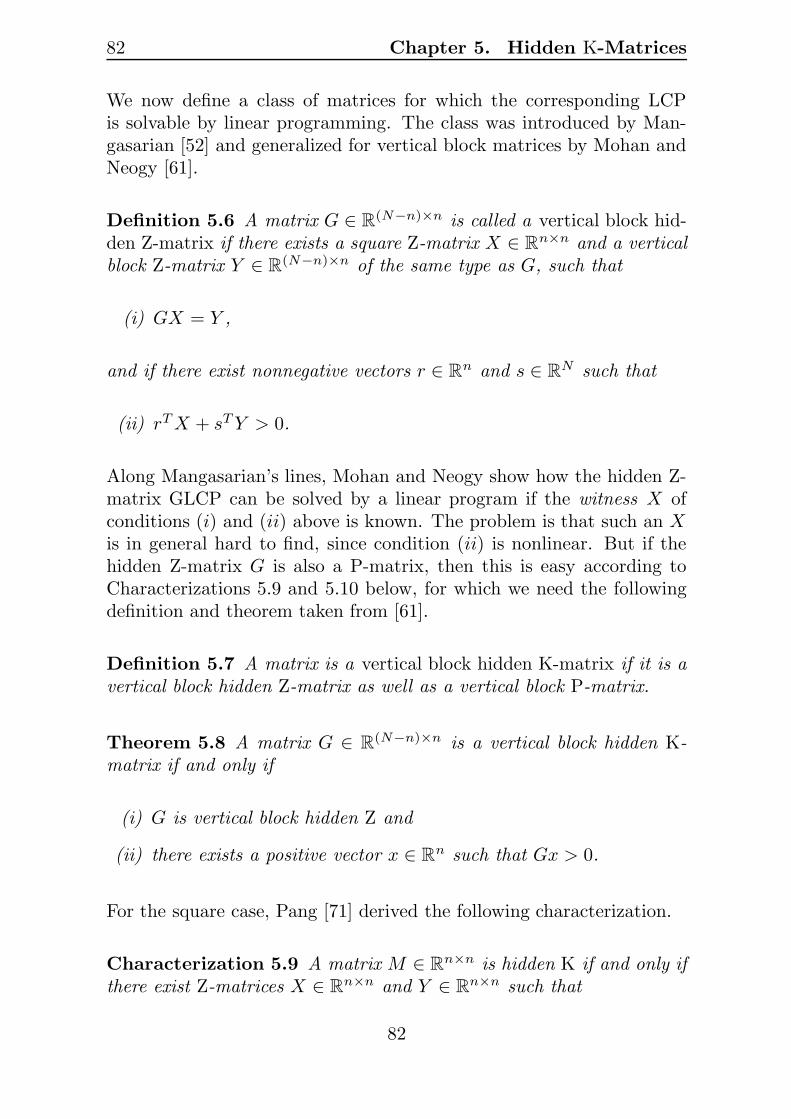
82 Chapter 5. Hidden K-Matrices
We now define a class of matrices for which the corresponding LCPis solvable by linear programming. The class was introduced by Man-gasarian [52] and generalized for vertical block matrices by Mohan andNeogy [61].
Definition 5.6 A matrix G ∈ R(N−n)×n is called a vertical block hid-
den Z-matrix if there exists a square Z-matrix X ∈ Rn×n and a vertical
block Z-matrix Y ∈ R(N−n)×n of the same type as G, such that
(i) GX = Y ,
and if there exist nonnegative vectors r ∈ Rn and s ∈ R
N such that
(ii) rTX + sTY > 0.
Along Mangasarian’s lines, Mohan and Neogy show how the hidden Z-matrix GLCP can be solved by a linear program if the witness X ofconditions (i) and (ii) above is known. The problem is that such an Xis in general hard to find, since condition (ii) is nonlinear. But if thehidden Z-matrix G is also a P-matrix, then this is easy according toCharacterizations 5.9 and 5.10 below, for which we need the followingdefinition and theorem taken from [61].
Definition 5.7 A matrix is a vertical block hidden K-matrix if it is avertical block hidden Z-matrix as well as a vertical block P-matrix.
Theorem 5.8 A matrix G ∈ R(N−n)×n is a vertical block hidden K-
matrix if and only if
(i) G is vertical block hidden Z and
(ii) there exists a positive vector x ∈ Rn such that Gx > 0.
For the square case, Pang [71] derived the following characterization.
Characterization 5.9 A matrix M ∈ Rn×n is hidden K if and only if
there exist Z-matrices X ∈ Rn×n and Y ∈ R
n×n such that
82

5.1. Matrix Classes 83
(i) MX = Y ,
(ii) Xe > 0, where e ∈ Rn is the all-one vector, and
(iii) there exists a positive vector x ∈ Rn such that Mx > 0.
A positive vector x as in (iii) always exists for P-matrices [17], so (i) and(ii) are enough for a P-matrix to be hidden K. It is known that condition(iii) can be replaced by Y e > 0, see [93] and [65]. We generalize this tovertical block matrices.
Characterization 5.10 A vertical block matrix G ∈ R(N−n)×n is hid-
den K if and only if there exist Z-matrices X and Y as in (i) of Defi-nition 5.6 such that
(i) GX = Y ,
(ii) Xe > 0, and
(iii) Y e > 0, where e ∈ Rn is the all-one vector.
Proof. If G is vertical block hidden K, then one can prove [61] thatthere exists a positive vector v ∈ R
n such that for the witnesses X andY in Definition 5.6 it holds that Xv > 0 and Y v > 0. Replacing X byXD and Y by Y D where D ∈ R
n×n is the diagonal matrix diag(vT ),the Z-matrix property is preserved and conditions (i), (ii) and (iii) aresatisfied.
For the other direction, assume that conditions (i)−(iii) hold. Con-dition (ii) assures by Lemma 5.5 that the Z-matrix X is a P-matrix.Its transpose, XT , is therefore also a P-matrix and as noted before, itis well-known that a positive vector r ∈ R
n exists such that XT r > 0.Using (i) and setting s ∈ R
N to zero we get that G is a hidden Z-matrixby Definition 5.6. By Theorem 5.8 it remains to show that Y e > 0implies existence of a vector x ∈ R
n such that Gx > 0. This is achievedby setting x to be the positive vector Xe, since Gx = GXe = Y e > 0.�
The nice thing about hidden K-matrices is that the witness P-matrixX can be found by solving a linear program. Since hidden K-matrices
83

84 Chapter 5. Hidden K-Matrices
(and their witnesses) are closed under scaling, the strict positivity con-straints in Characterization 5.10 can easily be realized by nonnegativityconstraints using standard tricks [71], see also Section 5.3.
Pang showed that square hidden K-matrices are closed under princi-pal pivot transforms [70]. We conclude this section by generalizing thisresult to vertical block matrices. Principal pivot transforms for verticalblock matrices have been defined for example in [39].
Theorem 5.11 Let G′ be a vertical block matrix derived from G bydoing a principal pivot transform. Then G′ is hidden K if and only ifG is hidden K.
Proof. A PPT corresponds to an interchange of variables in the equa-tion
w −Gz = q (5.12)
of the GLCP. Let’s without loss of generality look at the PPT thatinterchanges variables w1
1 and z1 and let’s assume (by scaling G and q)that the entry G1
11 is 1. The first row of (5.12) tells us that w11 − z1 −
G112z2 − . . . − G1
1nzn = q11 . After the PPT, the first row of (5.12) willbe z1 − w1
1 + G112z2 + . . . + G1
1nzn = −q11 and all occurrences of z1 inthe other rows will be replaced by w1
1 −G112z2 − . . .−G1
1nzn (we forgetabout the −q11 term, since it affects the right-hand side of the GLCPand we are interested in G′ only). The matrix G′ derived by this PPTis therefore G∗T where G∗ is G with the first row replaced by the firstrow of the n× n identity matrix and T ∈ R
n×n is
1 −G112 −G1
13 . . . −G11n
0 1 0 . . . 00 0 1 . . . 0...
......
. . ....
0 0 0 . . . 1
.
The inverse of T is
1 G112 G1
13 . . . G11n
0 1 0 . . . 00 0 1 . . . 0...
......
. . ....
0 0 0 . . . 1
.
84

5.2. Hidden K-Matrix GLCP and LP 85
The first row of T−1 is exactly the first row of G. Let X be the hiddenK witness of G and Y = GX as in Characterization 5.10. Then T−1Xis a hidden K witness for G′ since
(i) G′T−1X = G∗TT−1X = G∗X is a Z-matrix because the first rowis the first row of X and the other rows are the same as in Y , and
(ii) T−1X is Z and T−1Xe > 0 because the first row of T−1X is thefirst row of Y (Y is Z and Y e > 0), and because the other rowsare the same as in X (X is Z and Xe > 0).
In general, let G be hidden K with witnesses X and Y and let G′ bederived through a PPT interchanging variables zi and wij (i ∈ [n] andj ∈ [gi]). Then G′ is hidden K with witnesses X ′ and Y ′, where X ′ isX with the ith row replaced by the jth row of Y i, and Y ′ is Y with thejth row of Y i replaced by the ith row of X. �
5.2 Hidden K-Matrix GLCP and LP
Here comes the central theorem in hidden Z-matrix theory. It’s provedin [61] by a straightforward generalization of the square case, one direc-tion of which was proved in [19] and the other in [72], using the theorydeveloped in Mangasarian’s papers [52, 54, 55]. We state it for hiddenK-matrices, i.e., we restrict it to P-matrices.
Theorem 5.13 Let G ∈ R(N−n)×n be a vertical block P-matrix and q
any (N−n) vector. There is a vector p ∈ Rn (independent from q) such
that the GLCP(G, q) has the same solution z as the linear program
minimize pT zsubject to Gz + q ≥ 0
z ≥ 0(5.14)
if and only if G is hidden K. If G is hidden K w.r.t. witness X, then pcan be chosen as any n-vector for which XT p > 0.
As mentioned in the proof of Characterization 5.10, X is a P-matrixand it is well-known that a vector p with XT p > 0 thus exists. Note
85

86 Chapter 5. Hidden K-Matrices
that the constraints of the LP (5.14) assure that w and z in the GLCPare nonnegative. The theorem states that for a hidden K-matrix G andsuitable p, the LP gives us complementarity of w and z for free.
In this section, we reprove one direction of the theorem. Using thenotion of a Π-compatible linear program derived in Section 2.2, we showthat the GLCP(G, q) with hidden K-matrix G can be solved by (5.14).Moreover, we prove that the grid USO arising from the hidden K-matrixGLCP (Section 3.1) and the orientation of the following linear programare the same (the orientation derived from a linear program will bedefined later).
minimize qTxsubject to GTx ≤ p
x ≥ 0,
where p is any vector such that XT p > 0 (X a hidden K witness ofG). This linear program is in fact the dual to (5.14) and it is in turnequivalent to
minimize
(0q
)T (x′
x
)
subject to (I |GT )
(x′
x
)
= p,(x′
x
)
≥ 0,
(5.15)
where 0 is the vector of all 0’s of appropriate size and x′ an n-vector ofslack variables. We still require XT p > 0.
We induce a partition Π on the set [N ] of column indices of (I |GT )by letting Πi be the set of column indices corresponding to the rows ofGi (the ith block of G) plus the index i of column I{i} (the ith columnof I). A representative set β is then a set having exactly one elementout of each block of Π and (I |GT )β is the matrix (I |GT ) restricted tocolumns in β.
In the following, we will write ATα with the interpretation (AT )αfor some matrix A. For every β, (I |GT )β is equal to (Iα||GTα) forsome representative submatrix G of G and some α ⊆ [n]. It’s an easyobservation that every representative submatrix G of the hidden K-matrix G is hidden K w.r.t. the same witness X. For such a submatrix,let Y = GX.
86
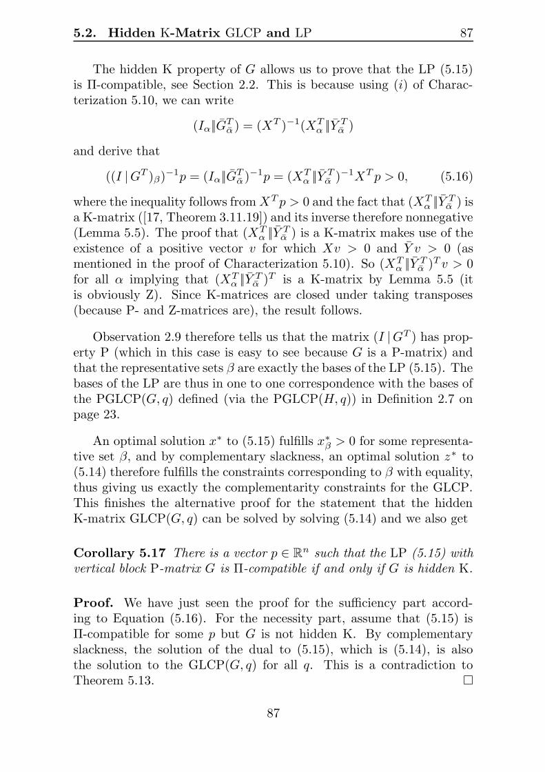
5.2. Hidden K-Matrix GLCP and LP 87
The hidden K property of G allows us to prove that the LP (5.15)is Π-compatible, see Section 2.2. This is because using (i) of Charac-terization 5.10, we can write
(Iα||GTα) = (XT )−1(XTα ||Y Tα )
and derive that
((I |GT )β)−1p = (Iα||GTα)−1p = (XT
α ||Y Tα )−1XT p > 0, (5.16)
where the inequality follows fromXT p > 0 and the fact that (XTα ||Y Tα ) is
a K-matrix ([17, Theorem 3.11.19]) and its inverse therefore nonnegative(Lemma 5.5). The proof that (XT
α ||Y Tα ) is a K-matrix makes use of theexistence of a positive vector v for which Xv > 0 and Y v > 0 (asmentioned in the proof of Characterization 5.10). So (XT
α ||Y Tα )T v > 0for all α implying that (XT
α ||Y Tα )T is a K-matrix by Lemma 5.5 (itis obviously Z). Since K-matrices are closed under taking transposes(because P- and Z-matrices are), the result follows.
Observation 2.9 therefore tells us that the matrix (I |GT ) has prop-erty P (which in this case is easy to see because G is a P-matrix) andthat the representative sets β are exactly the bases of the LP (5.15). Thebases of the LP are thus in one to one correspondence with the bases ofthe PGLCP(G, q) defined (via the PGLCP(H, q)) in Definition 2.7 onpage 23.
An optimal solution x∗ to (5.15) fulfills x∗β > 0 for some representa-tive set β, and by complementary slackness, an optimal solution z∗ to(5.14) therefore fulfills the constraints corresponding to β with equality,thus giving us exactly the complementarity constraints for the GLCP.This finishes the alternative proof for the statement that the hiddenK-matrix GLCP(G, q) can be solved by solving (5.14) and we also get
Corollary 5.17 There is a vector p ∈ Rn such that the LP (5.15) with
vertical block P-matrix G is Π-compatible if and only if G is hidden K.
Proof. We have just seen the proof for the sufficiency part accord-ing to Equation (5.16). For the necessity part, assume that (5.15) isΠ-compatible for some p but G is not hidden K. By complementaryslackness, the solution of the dual to (5.15), which is (5.14), is alsothe solution to the GLCP(G, q) for all q. This is a contradiction toTheorem 5.13. �
87

88 Chapter 5. Hidden K-Matrices
We note that p can be chosen to be positive (because XT is a P-matrix). For a square hidden K-matrix MT , according to (5.16), pfulfills
(Iα||Mα)−1p > 0
for all α. Up to reshuffling rows and/or columns, this is equivalent to
(Iα,α −Mα,α(Mα,α)−1
0α,α (Mα,α)−1
)
p > 0
for all α, where 0 is the matrix of all zeros and the notation Aα,α′ forα, α′ ⊆ [n] denotes the matrix we get from A ∈ R
n×n if we restrict torows with indices in α and columns with indices in α′. The positivevector p thus satisfies the following property:
(Mα,α)−1pα > 0 for all α. (5.18)
By making use of this positive vector p, Lemke’s algorithm solvesthe LCP(M, q) in at most n iterations [14]. Our result states that ifMT is hidden K, then a positive vector p fulfilling (5.18) exists andthe LCP(M, q) can therefore be solved in n steps of Lemke’s algorithm.This has been proved before [73], and the converse is also known [62](if a p fulfilling (5.18) exists, then MT is hidden K).
We now proceed to show that the orientations underlying the hiddenK GLCP and the LP (5.15) are the same. As noted above, the basesβ of the LP are in one to one correspondence with the bases of thePGLCP(H, q) which implies that the underlying grid graph is the same.According to (3.3) on page 31, the orientation of edges incident to vertexβ in the PGLCP(H, q) can be read off the (N − n)-dimensional vectorB(β)−1q, where a negative component corresponds to an outgoing edgeand a positive component to an incoming edge. For the LP (5.15) it isknown that the reduced cost vector
c(β) :=
(0q
)
β
−(
IG
)
β,[n]
((IG
)
β,[n]
)−1 (0q
)
β
(5.19)
encodes the orientation at vertex β in the same way, see for exampleChvatal’s book [10]. It thus suffices to prove that c(β) = B(β)−1q. Forthat we fix a basis β and define kI to be the number of columns of theidentity matrix in (I |GT )β . Similarly, kG is the number of columns
88

5.2. Hidden K-Matrix GLCP and LP 89
of the matrix GT in (I |GT )β . It holds that kI + kG = n. For nota-tional convenience we assume without loss of generality that the matrix
(I |GT ) (and the vector
(0q
)
) is sorted according to β, meaning that
the first kI columns in I (entries in the vector 0) and the first kG columnsin GT (entries in q) are those covered by β. Moreover, we define [kI ]to be the set [n] \ [kI ] and [kG] to be the set [N − n] \ [kG]. Notethat [kI ] consists of kG elements. In the following, we omit informationconcerning the dimensions of the identity- and zero-matrices, but thereader is able to figure out from the context of which dimension thematrices/vectors are. Equation (1) below holds because
(
I[kI ],[kI ] 0[kI ],[kI ]
G[kG],[kI ] G[kG],[kI ]
)−1
=
(
I[kI ],[kI ] 0[kI ],[kI ]
−(G[kG],[kI ])−1G[kG],[kI ] (G[kG],[kI ])
−1
)
.
c(β) =
(0q
)
β
−(
IG
)
β,[n]
((IG
)
β,[n]
)−1 (0q
)
β
=
(0q
)
β
−(
IG
)
β,[n]
(I[kI ],[n]
G[kG],[n]
)−1 (0[kI ]
q[kG]
)
=
(0q
)
β
−(
IG
)
β,[n]
(
I[kI ],[kI ] 0[kI ],[kI ]
G[kG],[kI ] G[kG],[kI ]
)−1(0[kI ]
q[kG]
)
(1)=
(0q
)
β
−(
IG
)
β,[n]
(0[kI ]
(G[kG],[kI ])−1q[kG]
)
=
(0q
)
β
−(
0[kI ],[kI ] I[kI ],[kI ]
G[kG],[kI ] G[kG],[kI ]
)(0[kI ]
(G[kG],[kI ])−1q[kG]
)
=
(
0[kI ]
q[kG]
)
−(
(G[kG],[kI ])−1q[kG]
G[kG],[kI ]
(G[kG],[kI ]
)−1q[kG]
)
=
(
−(G[kG],[kI ])−1 0[kI ],[kG]
−G[kG],[kI ](G[kG],[kI ])−1 I[kG],[kG]
)(q[kG]
q[kG]
)
=
(
−G[kG],[kI ]
0[kI ],[kG]
−G[kG],[kI ] I[kG],[kG]
)−1 (q[kG]
q[kG]
)
= (Hβ)−1q = B(β)−1q,
89

90 Chapter 5. Hidden K-Matrices
where the sorting of (I |GT ) according to β resulted in H being (G | I)in the PGLCP(H, q) with the first columns in G and I ∈ R
(N−n)×(N−n)
being the ones covered by β.
An LP orientation is acyclic, since following an outgoing edge meansimproving the objective function. We have thus proved
Theorem 5.20 The grid-orientation (given by (3.3)) of the GLCP withhidden K-matrix G and right-hand side vector q is the same as theacyclic grid-orientation (given by the reduced cost vector in (5.19)) ofthe linear program (5.15).
So the orientation induced by a hidden K-matrix GLCP is acyclic forevery q. The converse is in general not true. In the following subsectionwe give a family of examples of P-matrices whose members are nothidden K and for which there is no q yielding a cyclic orientation. Werefer to a q yielding a cyclic orientation as a cyclic q in the following.
5.2.1 A Family of Acyclic Non Hidden K-Matrices
We show that the following family of square matrices are P-matricesthat are not hidden K and for which there is no cyclic q, if the entriesa, b, c are chosen in a suitable way.
M1 =
( 1 a 00 1 bc 0 1
)
Matrices in this family generalize the matrix of [87] yielding a cyclic3-cube USO (we get this matrix by setting a = b = c = 2). We restrictour analysis to P-matrices in this family. M1 is a P-matrix if and onlyif its determinant 1 + abc is positive.
Lemma 5.21 The P-matrix M1 is a hidden K-matrix if and only ifone of the following is true.
1. At least one of the three entries a, b, c is nonpositive.
2. All entries a, b, c are positive and abc < 1.
90

5.2. Hidden K-Matrix GLCP and LP 91
Proof. If all three entries a, b, c are nonpositive, then M1 is a Z-matrixand therefore a (hidden) K-matrix. For the other cases, we use thatconditions (i) and (ii) of Characterization 5.9 are enough for a P-matrixto be hidden K. If exactly two entries are nonpositive (let’s say a andb, wlog), then the following X is a hidden K witness:
( 1 0 0bc 1 − bc 0−c 0 1 + c
)
.
For exactly one entry being nonpositive (let’s say a, wlog), the followingX is a hidden K witness:
(1 − ab 0 ab(1 + c)
0 1 + b+ bc −b(1 + c)−c(1 − ab) 0 1 + c
)
.
It remains to show that in the case where a, b and c are positive, M1 ishidden K if and only if abc < 1. If abc < 1 then the following X is awitness for M1 being hidden K.
(1 + a+ ab −a(1 + b+ bc) 0
0 1 + b+ bc −b(1 + c+ ac)−c(1 + a+ ab) 0 1 + c+ ac
)
IfM1 is hidden K, then (i) and (ii) of Characterization 5.9 imply (amongothers) the two constraints
x12 + ax22 ≤ 0
x11 + x12 + x13 > 0
for a Z-matrix X. The second constraint implies that x11 + x12 > 0(since x13 ≤ 0; note that x12 ≤ 0 also implies x11 > 0). Togetherwith the first constraint this yields x11 > ax22. By the same argumentwe also get x22 > bx33 and x33 > cx11. Taking the three constraintstogether (and making use of a, b, c > 0) gives abc < 1. �
Lemma 5.22 The following two statements are equivalent.
1. There is a right-hand side vector q such that the LCP USO (givenby (3.3)) induced by the P-matrix M1 and q is cyclic.
91

92 Chapter 5. Hidden K-Matrices
��
��
Figure 5.2: The cyclic USO of the 3-cube.
2. All entries a, b, c of M1 are positive and abc > 1.
Proof. The only cyclic USO of the 3-dimensional cube (up to iso-morphic ones derived by rotation and reflection of the cube, see alsoSubsection 3.3.3) is the one given in Figure 5.2 [87]. Note that theorientation has the following two properties.
(P1) All 2-dimensional faces are bows, i.e. the sink and the source inthese faces are neighbors.
(P2) In every dimension, there are three edges having the same orien-tation and one edge going into the opposite direction.
Let q = (q1, q2, q3)T . The orientation induced by M1 is determined by
the following table, where B(α) are the basis matrices of the PLCP(M1, q)as defined in Definition 1.5 on page 14.
α (B(α)−1q)1 (B(α)−1q)2 (B(α)−1q)3{1, 2, 3} q1 q2 q3{2, 3} −q1 q2 −cq1 + q3{1, 3} q1 − aq2 −q2 q3{3} −q1 + aq2 −q2 −cq1 + acq2 + q3{1, 2} q1 q2 − bq3 −q3{2} −q1 bcq1 + q2 − bq3 cq1 − q3{1} q1 − aq2 + abq3 −q2 + bq3 −q3{} −q1 + aq2 − abq3 −bcq1 − q2 + bq3 cq1 − acq2 − q3
The entry q2 at position ({2, 3}, (B(α)−1q)2) for example tells usthat (B({2, 3})−1q)2 = q2. That is, according to (3.4), the edge starting
92

5.2. Hidden K-Matrix GLCP and LP 93
{2} {1,2}
{1}{}
{3} {1,3}
{2,3} {1,2,3}
{2} {1,2}
{1}{}
{3} {1,3}
{2,3} {1,2,3}
Figure 5.3: Construction of a cyclic orientation induced by M1.
at vertex {2, 3} is outgoing into the direction of the second dimension ifq2 < 0 and incoming if q2 > 0 (the ith dimension is the one along whichwe go when switching from vertex α to α⊕ i).
The entries in the row where α = {} are missing a positive (sinceM1 is a P-matrix) factor 1/(1 + abc). But since we will be interested inthe sign of the entries only, we left it away.
How does a q yielding a cycle look like? We can assume that q1 > 0,otherwise we look at −q which yields the orientation with every edgereversed and thus preserves cycles (q1 = 0 would yield a degenerateorientation). According to the table above, this fixes the orientationof the two edges in Figure 5.2.1 left. Also from the table, we can readthat the edges from {1, 2, 3} and {2, 3} into direction 2 have the sameorientation. The same holds for the edges from {1, 2, 3} and {1, 3} intodirection 3. This is indicated by an equality sign on the edges.
Properties (P1) and (P2) let us fix the edges from {1, 3} to {3} and{1} to {} in Figure 5.2.1 right. (P1) tells us that the edge from {3} to{} should have the same orientation as the one from {1, 3} to {1}. By(P1) again, the edge from {1, 2} to {1} has opposite direction to theedges with equality signs in dimension 2, which is equivalent (by (P2))to stating that the edge from {2} to {} gets an equality sign.
If the edges with equality signs in dimension 3 would all be directeddownwards (and the unique one without the equality sign upwards),then it wouldn’t be possible to set sink and source antipodal, becausethe only possibilities left for the sink would be {1} and {1, 2} and thevertices antipodal to them would both already have an incoming edge
93
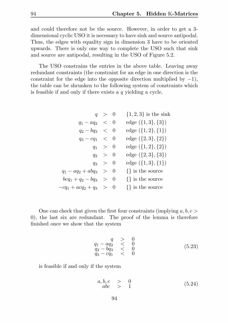
94 Chapter 5. Hidden K-Matrices
and could therefore not be the source. However, in order to get a 3-dimensional cyclic USO it is necessary to have sink and source antipodal.Thus, the edges with equality sign in dimension 3 have to be orientedupwards. There is only one way to complete the USO such that sinkand source are antipodal, resulting in the USO of Figure 5.2.
The USO constrains the entries in the above table. Leaving awayredundant constraints (the constraint for an edge in one direction is theconstraint for the edge into the opposite direction multiplied by −1),the table can be shrunken to the following system of constraints whichis feasible if and only if there exists a q yielding a cycle.
q > 0 {1, 2, 3} is the sink
q1 − aq2 < 0 edge ({1, 3}, {3})q2 − bq3 < 0 edge ({1, 2}, {1})q3 − cq1 < 0 edge ({2, 3}, {2})
q1 > 0 edge ({1, 2}, {2})q2 > 0 edge ({2, 3}, {3})q3 > 0 edge ({1, 3}, {1})
q1 − aq2 + abq3 > 0 {} is the source
bcq1 + q2 − bq3 > 0 {} is the source
−cq1 + acq2 + q3 > 0 {} is the source
One can check that given the first four constraints (implying a, b, c >0), the last six are redundant. The proof of the lemma is thereforefinished once we show that the system
q > 0q1 − aq2 < 0q2 − bq3 < 0q3 − cq1 < 0
(5.23)
is feasible if and only if the system
a, b, c > 0abc > 1 (5.24)
94
5.3. Non Hidden K-Matrices 95
is feasible. It’s easy to see that (5.23) implies (5.24). For the otherdirection, having a, b, c > 0 and abc > 1, the following q is feasible for(5.23):
q =
(ab+ a+ 1bc+ b+ 1ac+ c+ 1
)
.
�
Lemmas 5.21 and 5.22 imply that P-matrix M1 with a, b, c > 0 andabc = 1 is a non hidden K-matrix for which there does not exist a qyielding a cyclic orientation. This M1 is a boundary case, in the sensethat if one perturbs its entries only a little bit, it either becomes hiddenK or there appears a cycle for some q.
In the next section, we derive a characterization for vertical blocknon hidden K-matrices, a generalization of a characterization first shownin [65]. By strengthening the conditions in the characterization, we arethen able to determine a nontrivial subclass of 3-dimensional P-matricesfor which a cyclic q exists.
5.3 Non Hidden K-Matrices
We first state the linear program that arises from Characterization 5.10.It is feasible if and only if G is hidden K.
maximize 0
subject ton∑
j=1
Xij ≥ 1 for all i
n∑
l=1
GiklXlj ≤ 0 for all i, k and j 6= i
n∑
j=1
n∑
l=1
GiklXlj ≥ 1 for all i, k
Xij ≤ 0 for all i 6= j
(5.25)
By “for all i, k” we mean all i ∈ [n] and, depending on i, all k ∈[gi]. The index j is also in [n]. Note that by scaling the witness X in
95

96 Chapter 5. Hidden K-Matrices
Characterization 5.10, the constraints Xe > 0 (Y e > 0) are feasible ifand only if the constraints Xe ≥ 1 (Y e ≥ 1) are feasible. The second setof constraints in the above LP assures that Y i
kj ≤ 0 for all i, k and j 6= i,implying that Y is a Z-matrix, and the third set of constraints assuresthat Y e > 0. The linear program (5.25) is thus feasible if and only ifG ∈ R
(N−n)×n is a hidden K-matrix. Its dual is derived by linking thefirst n constraints to variables Rii for all i, the next (N − n)(n − 1)constraints to variables Sikj for all i, k and j 6= i, and the next (N − n)
constraints to variables Siki for all i, k. The S-variables thus form avertical block matrix of the same type as G.
min
nX
i=1
(Rii +
nX
k=1
Siki)
s.t. Rii +X
l6=j
glX
k=1
GlkiS
lkj +
nX
l=1
glX
k=1
GlkiS
lkl ≤ 0 for all i 6= j
Rii +X
l6=i
glX
k=1
GlkiS
lki +
nX
l=1
glX
k=1
GlkiS
lkl = 0 for all i
Rii ≤ 0, Siki ≤ 0 for all i, k
Sikj ≥ 0 for all i, k and j 6= i.
(5.26)
The first n2 − n constraints in (5.26) correspond to the variables Xij ,i 6= j, in (5.25) and the next n constraints to the variables Xii.
We replace variables Rii by −Rii and variables Sikj by −Sikj for alli, j, k, move some terms from the right double sum to the left doublesum, and get
max
nX
i=1
(Rii +
nX
k=1
Siki)
s.t. Rii +
nX
l=1
glX
k=1
GlkiS
lkj +
X
l6=j
glX
k=1
GlkiS
lkl ≥ 0 for all i 6= j
Rii +
nX
l=1
glX
k=1
GlkiS
lki +
X
l6=i
glX
k=1
GlkiS
lkl = 0 for all i
Rii ≥ 0, Siki ≥ 0 for all i, k
Sikj ≤ 0 for all i, k and j 6= i.
By defining R′ and S′ to be the matrices with R′ij := Rii and
S′ikj :=
{
Siki if j 6= i0 if j = i
96
5.3. Non Hidden K-Matrices 97
for all i, j, k, the previous LP can be written as
maximize
n∑
i=1
(Rii +
n∑
k=1
(Siki + S′iki))
subject to R′ +GT (S + S′) = T
Rii ≥ 0, Siki ≥ 0, Tii = 0 for all i, k
Sikj ≤ 0, Tij ≥ 0 for all i, k and j 6= i.
Replacing S + S′ by a new matrix S and merging the constraints forthe matrix R′ and the slack matrix T into constraints for the matrix R,we can equivalently state this as
maximize
n∑
i=1
(Rii +
n∑
k=1
Siki)
subject to R+GTS = 0
Rii ≥ 0, Siki ≥ 0 for all i, k
Rij ≤ Rii, Sikj ≤ Siki for all i, k and j 6= i.
(5.27)
Since (5.27) is always feasible, it is unbounded if and only if (5.25) isinfeasible (a standard fact in linear programming theory) which is inturn the case if and only if G is not hidden K. We therefore get thefollowing characterization for non hidden K-matrices:
Characterization 5.28 A vertical block matrix G ∈ R(N−n)×n of type
(g1, . . . , gn) is not hidden K if and only if
(i) R+GTS = 0 for some matrix R ∈ Rn×n and some vertical block
matrix S of the same size and type as G with
(ii) Rii ≥ 0, Siki ≥ 0, Rii ≥ Rij , Siki ≥ Sikj for all i, j ∈ [n] and k ∈ [gi],
and
(iii) at least one diagonal element of R or at least one diagonal elementof some representative submatrix of S is nonzero.
For the remainder of this chapter, we focus on square matrices. Thespecialization of Characterization 5.28 to square matrices is:
97

98 Chapter 5. Hidden K-Matrices
Characterization 5.29 A matrix M ∈ Rn×n is not hidden K if and
only if
(i) R+MTS = 0 for some matrices R and S in Rn×n with
(ii) Rii ≥ 0, Sii ≥ 0, Rii ≥ Rij , Sii ≥ Sij for all i, j, and
(iii) at least one diagonal element of R or S is nonzero.
This is the same characterization for square matrices as the one givenin [65], except that condition (iii) is replaced by:
(iii′) R and S are not both zero.
However, if R and S satisfy (i), (ii) and (iii′), then the matrices R′
and S′ we get from R and S by post-multiplying them with the squaren × n matrix with all off-diagonal entries being −1 and all diagonalentries being n satisfy (i), (ii) and (iii). The two characterizations aretherefore equivalent.
The characterization of [65] has been derived using different meth-ods than dualization of linear programs. Characterization 5.29 can betightened for minimal non hidden K P-matrices.
Definition 5.30 A square non hidden K matrix is called minimal if allproper principal submatrices of all principal pivot transforms are hiddenK-matrices.
Given a P-matrix M that is minimal non hidden K with witnessesR and S as in Characterization 5.29, we first show that S does nothave a row with all entries being zero. For that remember the nota-tion Aα,α′ introduced on page 88. Assume for contradiction that theith row of S is zero. Then R[n]\i,[n]\i and S[n]\i,[n]\i are witnesses forM[n]\i,[n]\i being non hidden K and therefore yield a contradiction tominimality, given that at least one diagonal element of R[n]\i,[n]\i orS[n]\i,[n]\i is nonzero. This is indeed the case: assume for contradictionthat all diagonal elements in R and S are zero, except Rii. By (ii) inCharacterization 5.29, the ith column of S is nonpositive (S{i} ≤ 0 andSii = 0), and R{i} = −MTS{i} ≤ 0 at all components except Rii. M
T
98

5.3. Non Hidden K-Matrices 99
then reverses the sign of the nonzero (because Rii 6= 0) vector S{i},meaning that (S{i})j(M
TS{i})j ≤ 0 for all j ∈ [n]. The existence ofthis sign reversing vector is well-known [17] to contradict the P-matrixproperty of MT and with this also of M . We conclude that S has nozero row.
All we needed to prove that S has no zero row was minimality andthe P-matrix property of M which implies that no sign reversing vectorexists. By pre-multiplying R + MTS = 0 with (M−1)T we get S +(M−1)TR = 0. Since the inverse of a minimal P-matrix is again aminimal P-matrix (the inverse is derived by a PPT), and since R andS share the same properties, this situation is completely symmetric tothe original one and we can prove along the same lines that R can nothave a zero row as well.
By post-multiplying R and S with the square n× n matrix with alloff-diagonal entries being −1 and all diagonal entries being n, we getnew R and S matrices with all diagonal entries being strictly positive,while R and S keep the properties of Characterization 5.29. We thusderive
Lemma 5.31 For a minimal non hidden K P-matrix M ∈ Rn×n the
witnesses R ∈ Rn×n and S ∈ R
n×n as in Characterization 5.29 donot have zero rows. Moreover, there exist R and S matrices with thefollowing properties.
(i) R+MTS = 0,
(ii) Rii > 0, Sii > 0, for all i and
(iii) Rii ≥ Rij , Sii ≥ Sij , for all i, j.
We note that it is known that every 3-dimensional P-matrix that isnot hidden K is minimal, since all P-matrices of dimension at most 2are hidden K. For general minimal non hidden K P-matrices it is notpossible to find witnesses R and S satisfying the constraints (iii) withstrict inequalities. We give an example of a minimal non hidden K P-matrix for which no R and S with strict constraints exist in the nextsubsection.
99
100 Chapter 5. Hidden K-Matrices
5.3.1 A Nontrivial Subclass
The example in Subsection 5.2.1 proves that there are non hidden K-matrices for which there exists no cyclic q. The question is how to tellmatrices with cyclic q-vectors and others apart. Looking at Lemma 5.31,a first idea might be to tighten all the constraints in Characteriza-tion 5.28. We define the following nontrivial and large subclass of nonhidden K-matrices.
Definition 5.32 A matrix M ∈ Rn×n is strongly not hidden K if
(i) R+MTS = 0 for some matrices R and S in Rn×n with
(ii) Rii > 0, Sii > 0, Rii > Rij , Sii > Sij for all i and j, i 6= j.
A non hidden K-matrix not fulfilling (i) and (ii) is weakly not hiddenK.
One might hope that strongly not hidden K-matrices are exactly thosenon hidden K-matrices which have a cyclic q. Although this could betrue in 3 dimensions (see also the next subsection) where we don’t havea counterexample, it is not true in general: the 4-dimensional P-matrix
M2 =
45 −44 81 −976 17 −21 81−76 9 83 −81−83 −79 61 53
is minimal weakly not hidden K (checked by computer) and there existcyclic q-vectors, an example is
q =
1632
.
The matrix M2 was found by Maple doing a brute force search (usingthe LP formulation arising from Lemma 5.36 below) and q was foundby a C++ program computing all the possible cells generated by thehyperplanes containing the 3-dimensional intersections of the comple-mentary 4-dimensional cones of the PGLCP (only later we were pointed
100
5.3. Non Hidden K-Matrices 101
to an existing software doing this: TOPCOM, written by Jorg Rambau[76] and available on the web).
We need some definitions in order to give a certificate for the factthat the above matrix M2 is weakly not hidden K.
Definition 5.33 A matrix M ∈ Rn×n is a Z◦-matrix if all off-diagonal
entries are negative.
Definition 5.34 A matrix M ∈ Rn×n is strongly hidden K if there
exist Z◦-matrices X ∈ Rn×n and Y ∈ R
n×n such that
(i) MX = Y ,
(ii) Xe > 0, and
(iii) Y e > 0, where e ∈ Rn is the all-one vector.
One can prove [65] that a matrix is hidden K if and only if it is stronglyhidden K, so the two classes are in fact the same.
Definition 5.35 A matrix M ∈ Rn×n is weakly hidden K if there exist
Z-matrices X ∈ Rn×n and Y ∈ R
n×n, X nonzero, such that
(i) MX = Y ,
(ii) Xe ≥ 0, and
(iii) Y e ≥ 0, where e ∈ Rn is the all-one vector.
Lemma 5.36 A matrix M ∈ Rn×n is strongly not hidden K if and
only if it is not weakly hidden K. The matrices in Rn×n are therefore
partitioned into three classes:
(1) (strongly) hidden K-matrices,
(2) strongly not hidden K-matrices,
(3) matrices that are weakly hidden K as well as weakly not hidden K.
101

102 Chapter 5. Hidden K-Matrices
Proof. According to Definition 5.35, it is easy to see that the matrixM is not weakly hidden K if and only if the following LP is bounded(note that it is always feasible).
maximize∑n
i=1Xii + Yiisubject to MX = Y
Xe ≥ 0Y e ≥ 0Xij ≤ 0, Yij ≤ 0, for all i and j 6= i
(5.37)
On the other hand, according to Definition 5.32, M is strongly nothidden K if and only if the following LP is feasible (it is always bounded).
minimize 0subject to −∑n
k=1MkiSki = 1 + ai for all i−∑n
k=1MkiSkj ≤ ai for all i and j 6= iSii = 1 + bi for all iSij ≤ bi for all i and j 6= iai ≥ 0, bi ≥ 0 for all i
(5.38)
One can check that these two LPs are dual to each other, the constraintsMX = Y , Xe ≥ 0, Y e ≥ 0 in (5.37) correspond to variables −S, −a,−b in (5.38). From LP theory, we get that (5.37) is bounded if and onlyif (5.38) is feasible, which proves the lemma. �
The matrix M2 above belongs to class (3) of Lemma 5.36. It is weaklynot hidden K:
9576 −18088 9576 95762142 2142 −62695 2142−2646 19754 87300 −264610206 −19278 10206 10206
+MT2
0 0 −827 0−126 0 0 −126
0 −238 0 00 0 −333 0
= 0.
And it is weakly hidden K:
M2
81 0 0 −810 0 0 00 0 0 0
−76 0 0 76
=
4329 0 0 −43290 0 0 00 0 0 0
−10751 0 0 10751
.
These witness matrices can be found using the Maple hidden K libraryprovided by the author. Also, the above q can be tested to be cyclic forM2. This is done by solving a linear program that tries to find a flowof maximal value in the corresponding USO between source and sink.The value of the flow is infinite if there exists a cycle.
102

5.3. Non Hidden K-Matrices 103
5.3.2 Dimension 3
We prove that 3-dimensional strongly non hidden K P-matrices have acyclic q.
Theorem 5.39 Let M ∈ R3×3 be a non hidden K P-matrix for which
matrices R ∈ R3×3 and S ∈ R
3×3 with
(i) R+MTS = 0,
(ii) Rii > 0, Sii > 0,
(iii) Rii > Rij and Sii > Sij
for all i and j, i 6= j exist. Then S can be assumed to be invertible andq := (ST )−1e is cyclic (e is the 3-dimensional all-one vector), meaningthat the 3-cube USO arising from the PLCP(M, q) has a cycle.
Proof. Note first that the properties of R and S allow us to perturb Sby small amounts (and adjust R) while preserving R + MTS = 0 andthe strict inequality constraints. This implies existence of an invertibleS.
By pre-multiplying the equation w−Mz = q in the PLCP with ST ,we arrive at STw − STMz = ST q which evaluates according to (i) toSTw+RT z = ST q. This is not a standard PLCP anymore, but we stillhave bases α ⊆ [n] (determining which variables are to be set to zeroin order to fulfill the complementarity conditions) and basis matricesC(α) := (STα ||RTα ). The underlying USO stays the same, since
C(α)−1ST q = ((ST )−1C(α))−1q
= ((ST )−1(STα ||RTα ))−1q
= (Iα|| −Mα)−1q
= B(α)−1q,
or simply because for bases in the two settings it holds that STB(α) =C(α) which implies C(α)−1ST q = B(α)−1q (it’s clear that C(α) isregular).
103

104 Chapter 5. Hidden K-Matrices
Up to now, we haven’t used the fact that we are in 3 dimensions.But now we fix an α ⊆ [3] and define C := C(α). The matrix C consistsof some columns out of ST and some out of RT . We label its entries asfollows (
C11 C21 C31C12 C22 C32C13 C23 C33
)
,
because this way, the transposes are directly taken care of, and we haveCii > 0 and Cii > Cij for all i 6= j. We look at the orientations of edgesincident to the vertex α if q is (ST )−1e. We define q := C(α)−1ST q =C−1e. By Cramer’s rule, the components of q can be computed as
q1 =
det
(1 C21 C311 C22 C321 C23 C33
)
det(C),
q2 =
det
(C11 1 C31C12 1 C32C13 1 C33
)
det(C),
q3 =
det
(C11 C21 1C12 C22 1C13 C23 1
)
det(C).
Now take the two entries q1 and q2. Expanding the numerator in q1along column 2 yields
C21 (C32 − C33)︸ ︷︷ ︸
<0
+C22 (C33 − C31)︸ ︷︷ ︸
>0
+C23(C31 − C32) (5.40)
and expanding the numerator in q2 along column 1 yields
C11 (C33 − C32)︸ ︷︷ ︸
>0
+C12 (C31 − C33)︸ ︷︷ ︸
<0
+C13(C32 − C31). (5.41)
The terms in brackets are the same except for reversed signs in bothdeterminants. We do a case analysis on the sign of (C31 − C32) (notethat the signs of the other terms in brackets are determined by theproperty that Cii > Cij for all i 6= j). If (C31 − C32) ≤ 0 then (5.40)can be shown to be positive by making use of C21 < C22 and C23 < C22.With the same argument, (C31 − C32) > 0 implies positivity of (5.41).
104

5.3. Non Hidden K-Matrices 105
�� ����
��
������
��
��
� ���
−
−−
−
+
++
+
−
−−
−
+
++
+
−
−−
−
+
++
+
−
−−
−
+
++
+
−
−−
−
+
++
+
Figure 5.4: The cyclic USO enforced by the pattern.
So, if (5.40) is negative (it’s never zero by the nondegeneracy as-sumption), then (C31 − C32) > 0 which in turn implies that (5.41) ispositive. On the other hand, if (5.41) is negative, then (C31 −C32) ≤ 0implying that (5.40) is positive. This means that if det(C) > 0, then ifone of the edges in dimensions 1 and 2 adjacent to vertex α is outgoing,the other edge has to be incoming. And if det(C) < 0, then if one ofthe edges in dimensions 1 or 2 is incoming, the other edge has to beoutgoing. Since this argumentation works for any two indices of q andany set α, we get the following pattern for all α:
det(C(α)) > 0 An outgoing edge forces the other two to be incomingdet(C(α)) < 0 An incoming edge forces the other two to be outgoing
By the P-matrix property of M , it is easy to see that det(B(α)) ispositive if and only if α has an even number of elements. Determi-nants of basis matrices differing in one column therefore have oppo-site signs and since C(α) = STB(α) this is also true for C(α). Sosign(det(C(α))) 6= sign(det(C(α′))) whenever |α ⊕ α′| = 1. We il-lustrate this by pluses and minuses in Figure 5.4, meaning that thedeterminant of basis matrix C(α) is positive (negative) if there is a plus(minus) at vertex α.
By the pattern, the source has to sit at a minus-vertex, wlog theone at the bottom left corner in Figure 5.4. Since the source is unique,the other minus-vertices have to have one incoming and two outgoingedges. Look at the minus-vertex antipodal to the source in the front 2-dimensional facet (shaded in Figure 5.4). The edge pointing away fromthe facet has to be oriented as in the figure, since the other directionwould imply two sources (and two sinks) in the facet (by the pattern).The same argument holds for the remaining two minus-vertices, forcingthe sink to be antipodal to the source in the 3-cube. It’s easy to seethat the pattern forces the remaining edges to form a cycle, either theone given in the figure or the one with opposite direction. �
105
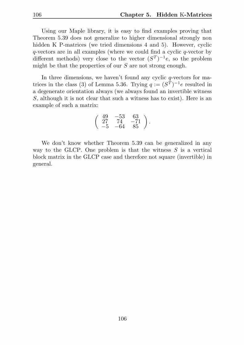
106 Chapter 5. Hidden K-Matrices
Using our Maple library, it is easy to find examples proving thatTheorem 5.39 does not generalize to higher dimensional strongly nonhidden K P-matrices (we tried dimensions 4 and 5). However, cyclicq-vectors are in all examples (where we could find a cyclic q-vector bydifferent methods) very close to the vector (ST )−1e, so the problemmight be that the properties of our S are not strong enough.
In three dimensions, we haven’t found any cyclic q-vectors for ma-trices in the class (3) of Lemma 5.36. Trying q := (ST )−1e resulted ina degenerate orientation always (we always found an invertible witnessS, although it is not clear that such a witness has to exist). Here is anexample of such a matrix:
(49 −53 6327 74 −71−5 −64 85
)
.
We don’t know whether Theorem 5.39 can be generalized in anyway to the GLCP. One problem is that the witness S is a verticalblock matrix in the GLCP case and therefore not square (invertible) ingeneral.
106

Chapter 6
Simple Stochastic Games
In this chapter, we show that the problem of finding optimal strate-gies for both players in a simple stochastic game (SSG) reduces to thePGLCP. This makes the rich PGLCP theory and algorithms availablefor SSG. As a special case, we get a reduction from binary SSG toPLCP.
SSG are two-player games on directed graphs, with certain randommoves. If both players play optimally, their respective strategies assignvalues v(i) to the vertices i, with the property that the first player winswith probability v(i), given the game starts at vertex i. For a givenstart vertex s, the optimization problem associated with the SSG isto compute the game value v(s); the decision problem asks whetherthe game value is at least 1/2. The formal setup of SSG is given inSection 6.1.
Section 6.2 then shows the actual reduction to PGLCP and con-cludes with an argument why P-matrices are probably more generalthan the matrices we get in SSG-induced PGLCPs. Section 6.3 givessome negative results, for example that the matrix in the SSG-inducedPGLCP is not a hidden K-matrix in general.
107

108 Chapter 6. Simple Stochastic Games
6.1 The Setup
We are given a finite directed graph G whose vertex set has the form
V = {1,0} ∪ Vmax ∪ Vmin ∪ Vavg,
where 1, the 1-sink, and 0, the 0-sink, are the only two vertices with nooutgoing edges.
Vertices in Vmax belong to the first player which we call the maxplayer, while vertices in Vmin are owned by the second player, the minplayer. Vertices in Vavg are average vertices. For i ∈ V \ {1,0}, welet N (i) be the set of neighbors of i along the outgoing edges of i.The elements of N (i) are {η1(i), . . . , η |N (i)|(i)}. An average vertex iis associated with a probability distribution P(i) that assigns to eachoutgoing edge (i, j) of i a probability pij > 0,
∑
j∈N (i) pij = 1.
The SSG defined by G is played by moving a token from vertex tovertex, until it reaches either the 1-sink or the 0-sink. If the token is atvertex i, it is moved according to the following rules.
vertex type rulei = 1 the game is over and the max player winsi = 0 the game is over and the min player winsi ∈ Vmax the max player moves the token to a vertex in N (i)i ∈ Vmin the min player moves the token to a vertex in N (i)i ∈ Vavg the token moves to a vertex in N (i) according to P(i)
A SSG is called stopping, if no matter what the players do, the tokeneventually reaches 1 or 0 with probability 1, starting from any vertex.In a stopping game, there are no directed cycles involving only verticesin Vmax ∪ Vmin. The following is well-known and has first been provedby Shapley [83], see also the papers by Condon [12, 13]. Our reductionyields an independent proof of part (i).
Lemma 6.1 Let G define a stopping SSG.
108

6.1. The Setup 109
(i) There are unique numbers v(i), i ∈ G, satisfying the equations
v(i) =
1, i = 10, i = 0
maxj∈N (i)
v(j), i ∈ Vmax
minj∈N (i)
v(j), i ∈ Vmin
∑
j∈N (i)
pijv(j), i ∈ Vavg
. (6.2)
(ii) The value v(i) is the probability for reaching the 1-sink from vertexi, if both players play optimally.
For a discussion about what it means that ‘both players play optimally’,we refer to Condon’s paper [13]. The important point here is thatcomputing the numbers v(i) solves the optimization version of the SSGin the sense that for every possible start vertex s, we know the valuev(s) of the game. It also solves the decision version which asks whetherv(s) ≥ 1/2. Additionally, the lemma shows that there are pure optimalstrategies that can be read off the numbers v(i): if v is a solution to(6.2), then an optimal pure strategy is given by moving from vertex ialong one outgoing edge to a vertex j with v(j) = v(i).
The stopping assumption can be made without loss of generality: ina non-stopping game, replace every edge (i, j) by a new average vertextij and new edges (i, tij) (with the same probability as (i, j) if i ∈ Vavg),(tij , j) with probability 1 − ε and (tij ,0) with probability ε. Optimalstrategies to this stopping game (which are given by the v(i) values)correspond to optimal strategies in the original game if ε is chosen smallenough [12].
Our original reduction is described in [34]. There we also assumethat the SSG is stopping, but we don’t insist on the replacement ofevery edge with the average vertices tij as above. Here we do that,which simplifies the reduction. Since consecutive average vertices canbe merged into one average vertex, we can assume bipartiteness of thegame graph, in the sense that all neighbors of player vertices are averagevertices and all neighbors of average vertices are player vertices or sinks.
109
110 Chapter 6. Simple Stochastic Games
6.2 Reduction from SSG to PGLCP
This section describes the core result of this chapter. As a help for thereader, we provide the reduction step by step for a specific example inSubsection 6.3.1.
In the following, G defines a bipartite, transformed (as describedabove) stopping SSG and every non-sink vertex of G has at least twooutgoing edges (a vertex of outdegree 1 can be removed from the gamewithout affecting the values of other vertices). In order to solve (6.2), wefirst write down an equivalent system of linear equations and inequali-ties, along with (nonlinear) complementarity conditions for certain pairsof variables. The system has one variable xi for each vertex i and oneslack variable wij for each edge (i, j) with i ∈ Vmax ∪ Vmin. It hasequality constraints
xi =
1, i = 10, i = 0
wij + xj , i ∈ Vmax, j ∈ N (i)−wij + xj , i ∈ Vmin, j ∈ N (i)∑
j∈N (i)
pijxj , i ∈ Vavg,
(6.3)
inequality constraints
wij ≥ 0, i ∈ Vmax ∪ Vmin, j ∈ N (i), (6.4)
and complementarity constraints
∏
j∈N (i)
wij = 0, i ∈ Vmax ∪ Vmin (6.5)
to model the max- and min-behavior in (6.2).
The statement of Lemma 6.1 (i) is equivalent to the statement thatthe system consisting of (6.3), (6.4) and (6.5) has a unique solutionx = (x1, . . . , xn), and we will prove the latter statement. Actually,we prove that the variables x are redundant and that there exists aunique solution for the variables w. From this we can recover the uniquesolution for the xi, which are the game values v(i). Note that edges withwij = 0 in the solution correspond to strategy edges of the players, i.e.,
110

6.2. Reduction from SSG to PGLCP 111
if wij = 0 then xi = xj and the best strategy for the player at vertex iis to move the token to vertex j.
In order to obtain a proper GLCP formulation, we remove the re-dundant x-variables (the fact that we can remove them implies thatthey are redundant). For variables xi, i /∈ Vavg, this is easy. For eachplayer vertex i we choose one arbitrary neighbor along an outgoing edgeand call it η1(i). In order to reveal connections to the final GLCP al-ready now, we call edges going from i to η1(i) z-edges and rename theirslack variables to zi, so zi := wiη1(i). Because of bipartiteness of thegame graph, every edge originating from a player vertex connects to anaverage vertex j. For i ∈ Vmax we can therefore replace all occurrencesof xi in (6.3) by zi + xη1(i), and for i ∈ Vmin by −zi + xη1(i), and endup with equalities consisting of xi for i ∈ Vavg only (x0 and x1 can bereplaced by 0 and 1 immediately):
wij − zi − xη1(i) + xj = 0, i ∈ Vmax, j ∈ N (i) \ η1(i)wij − zi + xη1(i) − xj = 0, i ∈ Vmin, j ∈ N (i) \ η1(i)
−xi +∑
j∈N (i)
pijSj = 0, i ∈ Vavg,(6.6)
where Sj in the last equation is zj + xη1(j) if j ∈ Vmax, −zj + xη1(j) ifj ∈ Vmin and 0 or 1 if j is a sink. Note that the right-hand sides of thefirst two equations are zero since player vertices do not connect to sinks(after the stopping transformation). Nevertheless, allowing connectionsfrom player vertices to sinks is no problem, resulting in constant valueson the right-hand side.
6.2.1 A Non-Standard GLCP
Let us assume that Vmax ∪ Vmin = {1, . . . , u}, Vavg = {u + 1, . . . , n}.We define vectors
z = (w1η1(1), . . . , wuη1(u))T = (z1, . . . , zu)
T
and
w = (w1, . . . , wu)T , x = (xu+1, . . . , xn)T ,
where wi = (wiη2(i), . . . , wiη |N(i)|(i)) is the vector consisting of the wijfor all j ∈ N (i)\η1(i). Conditions (6.4), (6.5) and (6.6) – and therefore
111
112 Chapter 6. Simple Stochastic Games
the problem of computing the v(i) – can now be written as
find w, zsubject to w, z ≥ 0
zi
|N (i)|−1∏
j=1
wij = 0, i ∈ Vmax ∪ Vmin
(w0
)
−(I CA B
)(zx
)
=(st
)
,
(6.7)
whereP =
(I CA B
)
, q =(st
)
are a suitable matrix and a suitable vector. The vertical block matrixI is partitioned according to w and all representative submatrices of itare the identity matrix in R
u×u. The square matrix B of dimensionn − u encodes the connections between average vertices along z-edges.A and C describe how player and average vertices interconnect.
6.2.2 The Structure of the Matrix P
After the transformation to stopping SSG and the merging of the av-erage vertices, all average vertices i have an escape-edge to the 0-sink,pi0 > 0. The matrix B is therefore row diagonally dominant with posi-tive diagonal entries, meaning that Bii >
∑
j 6=i |Bij |. This implies thatB is a P-matrix [93]. Since it is a Z-matrix by construction, it is evena K-matrix, see Definition 5.4.
Property 6.8 An (n× n) representative submatrix
P =(I CA B
)
of P is given by a representative submatrix I of I and C which consistsof the rows of C corresponding to the rows of I. P corresponds to asubgame where (non-z-)edges have been deleted such that every playervertex has exactly two outgoing edges.
Such a subgame is a slightly generalized binary SSG, since average ver-tices can have more than two outgoing edges and arbitrary probabilitydistributions on them.
112

6.2. Reduction from SSG to PGLCP 113
Lemma 6.9 Using elementary row operations, we can transform a rep-resentative submatrix P of P into a matrix P ′ of the form
P ′ =
(
I C0 B′
)
with B′ being a P-matrix.
Proof. We process the rows of the lower part (AB) of P one by one.In the following, we restrict to the subgame corresponding to P , whereall player vertices have two outgoing edges.
For k ∈ {1, . . . , n}, let Rk be the kth row of P and assume that weare about to process Ri, i ∈ {u+ 1, . . . , n}. According to (6.6), we have
Ri
(zx
)
= xi −∑
j∈N (i)\{0,1}
pij(±zj + xη1(j)), (6.10)
with +zj if j ∈ Vmax and −zj if j ∈ Vmin. We will eliminate thecontribution of ±zj +xη1(j) for all j ∈ N (i) \ {0,1}, by adding suitablemultiples of rows Rj , j ∈ {1, . . . , u}. For such a j, (6.6) implies
Rj
(zx
)
=
{zj + xη1(j) − xη2(j), j ∈ Vmaxzj − xη1(j) + xη2(j), j ∈ Vmin
,
where η2(j) is the second neighbor of j in the subgame corresponding toP . Thus, adding a fraction (either −pij or pij) of such a row to (6.10)for all j ∈ N (i)\{0,1} transforms our current matrix into a new matrixwhose ith row has changed and yields
R′i
(zx
)
= xi −∑
j∈N (i)\{0,1}
pijxη2(j). (6.11)
This transformation is realized through elementary row operations. Be-cause (6.11) does not contain any z-variables anymore, we get theclaimed structure after all rows Ri, i ∈ {u + 1, . . . , n}, have been pro-cessed.
B′ is again a P-matrix (even a K-matrix) since it is row diagonallydominant and positive on the diagonals. �
Lemma 6.12 P is a vertical block P-matrix.
113

114 Chapter 6. Simple Stochastic Games
Proof. We show that every representative submatrix P of P is a P-matrix. By Lemma 6.9, det(P ) = det(P ′) = det(I) det(B′) = det(B′),so P has positive determinant since B ′ is a P-matrix. To see that allproper principal minors are positive, we can observe that any principalsubmatrix of P is again the matrix resulting from a SSG. The subgamecorresponding to a principal submatrix can be derived from the SSG bydeleting vertices and redirecting edges. The deletion of a player vertexis described in Figure 6.1. Squares correspond to average and trian-
Figure 6.1: Removing a player vertex.
gles to player vertices. The dots indicate that there can be arbitrarilymany average vertices having a directed edge to the vertex we want todelete. The bold edge indicates the z-edge of the player vertex (remem-ber that player vertices in the subgame described by P have outdegree2). Strictly speaking, the resulting game is not bipartite anymore, butlooking through the reduction once more, we see that consecutive av-erage vertices are handled easily: there are in fact less entries in thesubmatrix A of P we have to get rid of in order to prove that P is aP-matrix along the lines of Lemma 6.9.
Figure 6.2 shows that the deletion of an average vertex is achievedby redirecting all incoming edges to the 0-sink. Since we now have sinksafter player vertices, the game is not of the original form anymore. Butagain, the reduction deals with that (some entries in the matrix C of Pare zero instead of 1 or −1 and the s-vector in (6.7) might no longer bezero, see also the remark after (6.6)) and the matrix corresponding tothe subgame has positive determinant. �
114

6.2. Reduction from SSG to PGLCP 115
PSfrag replacements0
Figure 6.2: Removing an average vertex.
6.2.3 A Standard GLCP
Problem (6.7) is a non-standard GLCP because there are variables xwith no complementarity conditions. But knowing that B is regular(since B is a P-matrix), we can express x in terms of z and obtain anequivalent standard GLCP.
find w, zsubject to w, z ≥ 0
zi
|N (i)|−1∏
j=1
wij = 0, i ∈ Vmax ∪ Vmin
w − (I − CB−1A)z = s− CB−1t
(6.13)
Lemma 6.14 The matrix I − CB−1A is a P-matrix.
Proof. We have to show that every representative submatrix of I −CB−1A is a P-matrix. Such submatrices are derived through I −CB−1A. It thus suffices to show that I − CB−1A is a P-matrix, giventhat P (as defined in Property 6.8) is a P-matrix. This is well-known,I − CB−1A is called the Schur complement of B in P (Tsatsomeros[92]). �
We therefore have
Theorem 6.15 A simple stochastic game is reducible in polynomialtime to a generalized linear complementarity problem with a P-matrix.
115

116 Chapter 6. Simple Stochastic Games
This theorem also provides a proof of Lemma 6.1: going through ourchain of reductions again yields that the equation system in Lemma 6.1(i) for the values v(i) has a unique solution if and only if the PGLCP(6.13) has a unique solution for the slack variables w and z. The latterholds because the matrix of (6.13) is a P-matrix, see Theorem 2.5.
As mentioned earlier in Section 1.1, the reduction works for a su-perclass of SSG in which edges are associated with a payoff. But forgeneral stochastic games as introduced by Shapley [83], our reductionis not possible. This follows from two facts. First, optimal strategiesfor stochastic games are generally non-pure. Second, it is possible toget irrational solutions (vertex values) for the stochastic game even ifall input data is rational [74]. This is not possible for GLCP.
Projecting the grid USO we get from a SSG-induced PGLCP todimensions of one player only (see [33, 32] for details about projectedUSOs), results in the acyclic grid USO that Bjorklund et al. derive viatheir reduction [3]. This phenomenon makes us believe that PGLCP ismore general than SSG since we don’t expect to observe it for generalP-matrices. We record this observation in a lemma.
Lemma 6.16 Consider a SSG-induced PGLCP instance. The gridUSO evolving from it has the property that there is at least one sub-set of dimensions (corresponding to one of the players in the SSG) suchthat the USO resulting from projecting w.r.t. the dimensions in the sub-set as well as the USO resulting from projecting w.r.t. all dimensionsnot in the subset is acyclic.
An interesting open question is whether the acyclic grid USOs of Bjork-lund et al. satisfy the Holt-Klee condition. The result that PGLCP-induced grid USO fulfill it does not answer the question in the affirma-tive, since the Holt-Klee property might get lost in a projected USO, seeFigure 1.1 on page 9 for an example. There, the left orientation is LP-induced and therefore satisfies the Holt-Klee condition while the right,projected orientation does not (it’s the double twist from Figure 3.2 onpage 34).
116
6.3. Negative Results 117
6.3 Negative Results
We show that the matrix in a SSG-induced PGLCP is in general not(transpose) hidden K and not positive semi-definite. Moreover, it is pos-sible that the SSG reduces to a PLCP that in turn reduces to a USO ofthe cube known as the Klee-Minty orientation. In such an orientation,there is a directed path visiting all vertices of the cube. A potential al-gorithm following this path would therefore need an exponential numberof steps to find the sink.
6.3.1 A SSG whose Matrix is not Hidden K
In order to illustrate the reduction, we provide an example here. More-over, the matrix we get through the reduction is not hidden K, thusdestroying one possible hope of getting a polynomial time algorithm forSSG via PGLCP. The example is an adaptation of Condon’s originalgame designed to show that switching algorithms can cycle [13]. Thecycle translates to the PGLCP USO in a straightforward way (switchingthe strategy at a player vertex is to move along one edge in the USO),which proves that the matrix is not hidden K (Theorem 5.20).
The reason we look at an adaptation and not at the original gameis that we also get a negative result in the setting of Svensson andVorobyov [88]. We come back to this after the reduction.
Figure 6.3 shows the SSG, with upper triangles denoting max playerand lower triangles denoting min player vertices. Squares are averagevertices and bold numbers correspond to sink values. The arrow point-ing to the bold number 9/10, for instance, is an abbreviation for anarrow pointing to an average vertex having two outgoing edges, one ofthem connecting to the 1-sink with probability 9/10 and the other con-necting to the 0-sink with probability 1/10. Since this average vertexwill have value 9/10, we can disregard it in the reduction (by replacingall occurrences of its x-variable by 9/10). The game consists of 4 playervertices, the resulting vertical block matrix in the PGLCP will thus beof dimension 4 (consist of 4 vertical blocks). We don’t know of anygame giving a 3-dimensional non hidden K-matrix.
We first write down the equations according to (6.3), nonnegativity
117
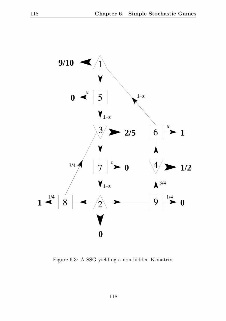
118 Chapter 6. Simple Stochastic Games
3/4
1/41/4
3/4
9/10
0
0
0 1/2
01
2/5
ε
1−ε
ε
1−ε
ε
1−ε
1
1
5
3
7
28 9
4
6
Figure 6.3: A SSG yielding a non hidden K-matrix.
118
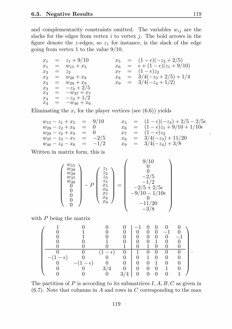
6.3. Negative Results 119
and complementarity constraints omitted. The variables wij are theslacks for the edges from vertex i to vertex j. The bold arrows in thefigure denote the z-edges, so z1 for instance, is the slack of the edgegoing from vertex 1 to the value 9/10.
x1 = z1 + 9/10 x5 = (1 − ε)(−z3 + 2/5)x1 = w15 + x5 x6 = ε+ (1 − ε)(z1 + 9/10)x2 = z2 x7 = (1 − ε)z2x2 = w28 + x8 x8 = 3/4(−z3 + 2/5) + 1/4x2 = w29 + x9 x9 = 3/4(−z4 + 1/2)x3 = −z3 + 2/5x3 = −w37 + x7x4 = −z4 + 1/2x4 = −w46 + x6
Eliminating the xi for the player vertices (see (6.6)) yields
w15 − z1 + x5 = 9/10 x5 = (1 − ε)(−z3) + 2/5 − 2/5εw28 − z2 + x8 = 0 x6 = (1 − ε)z1 + 9/10 + 1/10εw29 − z2 + x9 = 0 x7 = (1 − ε)z2w37 − z3 − x7 = −2/5 x8 = 3/4(−z3) + 11/20w46 − z4 − x6 = −1/2 x9 = 3/4(−z4) + 3/8
.
Written in matrix form, this is
w15w28w29w37w4600000
− P
z1z2z3z4x5x6x7x8x9
=
9/1000
−2/5−1/2
−2/5 + 2/5ε−9/10 − 1/10ε
0−11/20−3/8
with P being the matrix
1 0 0 0 −1 0 0 0 00 1 0 0 0 0 0 −1 00 1 0 0 0 0 0 0 −10 0 1 0 0 0 1 0 00 0 0 1 0 1 0 0 00 0 (1 − ε) 0 1 0 0 0 0
−(1 − ε) 0 0 0 0 1 0 0 00 −(1 − ε) 0 0 0 0 1 0 00 0 3/4 0 0 0 0 1 00 0 0 3/4 0 0 0 0 1
.
The partition of P is according to its submatrices I, A,B,C as given in(6.7). Note that columns in A and rows in C corresponding to the max
119

120 Chapter 6. Simple Stochastic Games
player have nonpositive entries (all the other entries are nonnegative).This fact assures that the matrix in the standard GLCP as in (6.13) isnonnegative:
w15w28w29w37w46
−
1 0 (1 − ε) 00 1 3/4 00 1 0 3/40 (1 − ε) 1 0
(1 − ε) 0 0 1
( z1z2z3z4
)
= q,
where
q =
1/2 + 2/5ε−11/20−3/8−2/5
2/5 + 1/10ε
.
This vertical block matrix of type (1, 2, 1, 1), as indicated by the hori-zontal lines, is easily seen to be a P-matrix, since both representativesubmatrices are row diagonally dominant with ones on the diagonal.The matrix has in fact a very simple structure. There are two reasonsfor that. The first is the choice of the z-edges in the reduction. Allof these edges lead directly to (sink) values. The second reason is thatthe game is tripartite, meaning that every max vertex is followed byaverage vertices that are followed by min vertices. These min verticesare followed by average vertices that are followed by max vertices.
Any SSG can without loss of generality be transformed in a tripartiteone where every player vertex is connected to a sink. This can beachieved by introducing additional vertices and introducing an edge tothe 1-sink for every min vertex and an edge to the 0-sink for every maxvertex. Such edges are called retreat edges and they are redundant, sinceit makes no sense for the players to choose such an edge. Applying thesame reduction as we do, Svensson and Vorobyov [88] show that on suchgames, the matrix in the final standard GLCP (the matrix I −CB−1Ain (6.13)) is a so called D-matrix. The drawback of reducing to a D-matrix is that binary SSG don’t reduce to LCP in general (since weintroduce the retreat edges). Here is the definition of D-matrices:
Definition 6.17 A vertical block matrix Q consisting of n blocks isa D-matrix if it is nonnegative, strictly row diagonally dominant andif there is a set α ⊆ [n] such that in every representative submatrixQ ∈ R
n×n
120

6.3. Negative Results 121
(i) there are ones on the diagonal, and
(ii) Qα,α and Qα,α are identity matrices of appropriate size.
Remember that Qα,α, as defined on page 88, is Q restricted to rowsand columns with indices in α. After having reduced SSG to D-matrixGLCP, the set α corresponds to the set of max player vertices. Thereader is encouraged to check that our matrix above is indeed a D-matrix for 0 < ε ≤ 1.
Every D-matrix is a P-matrix. It is interesting that every squareD-matrix Q is hidden K. A possible witness is X := 2I −Q, that is Qwith all off-diagonal entries turned into their negative values. Since Qis row diagonally dominant, we have Xe > 0 and according to Charac-terization 5.9 it thus suffices to check that QX is a Z-matrix. This iseasy.
Despite these nice properties, D-matrices are not hidden K in gen-eral. The matrix above is a counterexample for instance for ε = 1/100.This can be checked by formulating Characterization 5.28 as an LPthat can be solved for example by Maple. More elegantly, computingthe (2×3×2×2)-grid USO corresponding to the PGLCP derived above,we see that it is cyclic. The cycle corresponds exactly to Condon’s orig-inal cycling-sequence, i.e., it appears in a 4-dimensional subcube of thegrid. The size 3 of the second dimension in our example was only neededto reduce to a D-matrix. The changes we made to Condon’s examplewere to add a retreat edge for vertex 2 (this gives size 3 of the 2nddimension) and to insert the average vertices 5, 6, 7 to make the gametripartite.
The reader might wonder why the ε-edge of vertex 6 goes to the 1-sink, whereas the ε-edges of vertices 5 and 7 go to the 0-sink. Although,in order to solve the game, adding average vertices with an ε-edge to anysink value works if ε is small enough, the reason of the values here is toavoid a degenerate USO. Indeed, if we would direct the ε-edge of vertex6 to the 0-sink as well, the following two strategies would have the samevalues for all vertices (which is not a bad thing for SSG): choose thenon-z-edges for player vertices 1, 3, 4 and for vertex 2 the edge going to9 (first strategy) or the retreat edge (second strategy). This results inan undirected edge in the USO.
Our result that every submatrix being hidden K is not enough for
121

122 Chapter 6. Simple Stochastic Games
a vertical block matrix to be hidden K is a strengthening of the sameresult for vertical block Z-matrices by Mohan and Neogy [60].
Here is the solution to the above PGLCP with ε = 1/100:
w15w28w29w37w46
=
63/1250
7/40289/2000401/1000
,
( z1z2z3z4
)
=
011/20
00
.
From this we can read off that the optimal strategy is to choose thez-edge for all player vertices except vertex 2. There, the edge going tovertex 8 should be taken. Given this strategy, the values v(i) in (6.2),or equivalently the values xi in (6.3), can be computed and checked tofulfill the max and min constraints in (6.2).
The outgoing edges of a player vertex correspond to one block ofvariables in the PGLCP. The choice of the z-edges determines the z-variable in one block. If we choose different z-edges, then the newPGLCP we get can be derived by doing a principal pivot transform onthe old one (moving the z-variables at the right place). Since hidden K-matrices are closed under principal pivot transforms (Theorem 5.11), thematrix resulting from the SSG in Figure 6.3 is not hidden K independentof the choice of z-edges.
If we remove the edge going from vertex 2 to the 0-sink in Figure 6.3and choose the z-edge at vertex 2 to be the one going to vertex 8, thenthe reduction yields the square matrix
M =
1 0 (1 − ε) 00 1 −3/4 3/40 (1 − ε) (1/4 + 3/4ε) 0
(1 − ε) 0 0 1
and right-hand side vector
q =
1/2 + 2/5ε7/40
3/20 − 11/20ε2/5 + 1/10ε
.
Setting ε to 1/100, the USO arising from this LCP is cyclic, implyingthat the matrix M is not hidden K. Moreover, the transpose of M isnot hidden K either, so the polynomial time algorithms known for the
122

6.3. Negative Results 123
LCP(M, q) with MT being hidden K (see [17] and also the discussionon page 88) can not be used for solving games in general. The transposeof the above matrix M (with ε = 1/100) is not hidden K, because thefollowing matrix is a witness S as in Characterization 5.29 on page 98(witness R can be computed as −MS):
1 1 1 −6049729403
1 1 −503396 1
−3 1 1 11 −602
297 1 1
.
We finish the example by stating our negative findings as a lemma:
Lemma 6.18 Simple stochastic games do in general not reduce to PGLCPwith a hidden K-matrix or with the transpose of a hidden K-matrix.
6.3.2 A SSG whose Matrix is Ill-Conditioned
In his book [97], Ye presents an interior point method to solve PLCPin time polynomial in the input size, given that the condition numberof the P-matrix M is bounded by a polynomial in the dimension of M .The condition number of a P-matrix M is defined as
−λθ(M)
,
where λ is the smallest eigenvalue of (M +MT )/2 and
θ(M) = min||x||=1
maxjxj(M
Tx)j .
Note that θ(M) is always positive, since M is a P-matrix and does notreverse the sign of any nonzero vector [17]. We look at the game givenin Figure 6.4. Doing the reduction yields matrix
M =
(
1 1ε − 1
0 1
)
.
The smallest eigenvalue of (M +MT )/2 is λ = 32 − 1
2ε and θ(M) can beseen to be at most 1 by choosing x = (0, 1)T . The condition number isthen at least 1
2ε − 32 which is exponential in the dimension of M if 1/ε
is. Since ε can be chosen arbitrarily small, we get the following result.
123

124 Chapter 6. Simple Stochastic Games
0 0
0
0
1−ε
ε
εε
1−ε1−ε
Figure 6.4: A SSG yielding an ill-conditioned matrix.
124

6.3. Negative Results 125
0
1
Figure 6.5: A SSG yielding a Klee-Minty cube.
Lemma 6.19 Simple stochastic games do not reduce to PLCP withwell-conditioned matrix in general.
By Ye’s definition, every P-matrix with positive eigenvalues is well-conditioned. A matrix M ∈ R
n×n is positive semi-definite if xTMx ≥ 0for all x ∈ R
n. It’s an easy observation that M is positive semi-definiteif and only if (M +MT )/2 is as well. Moreover, it is known that a sym-metric matrix is positive semi-definite if and only if all eigenvalues arenonnegative (see [17] for example). Positive semi-definite P-matrices aretherefore well-conditioned and Ye’s algorithm solves such LCPs in poly-nomial time (polynomial time algorithms are also known for the LCPwith general positive semi-definite matrices [67]). The above lemmatherefore includes the result that simple stochastic games do not reduceto PLCP with positive semi-definite matrix in general.
6.3.3 Exponential Lower Bound for SSG
Melekopoglou and Condon give examples of binary SSG needing anexponential number of switches in the worst case [59]. Basically, such agame is a generalization of the example with 3 player vertices given inFigure 6.5, where edges at average vertices have probability 1/2.
Since switching an edge at a player vertex amounts to following anoutgoing edge in the corresponding PLCP USO, their result states that
125

126 Chapter 6. Simple Stochastic Games
the cube USO resulting from the game belongs to a class of orientationsdescribed by Klee and Minty in [48]. A necessary condition for membersin their class of orientations is the existence of a path from the source tothe sink visiting all vertices of the cube. And indeed, certain switchingalgorithms follow this path.
A Klee-Minty cube USO is actually generated by LP and was thefirst example to show that the simplex method with Dantzig’s pivotrule may require an exponential number of pivot steps [48]. For theexample of Figure 6.5, a longest possible switching sequence is givenin Figure 6.7. Numbers at vertices denote the vertex values for thestrategy determined by thick arrows.
Interestingly, the game uses only min player vertices. The path ofthe 3-cube USO, corresponding to the switching sequence, is given inFigure 6.6. Numbers at cube-vertices denote the strategy of Figure 6.7corresponding to the vertex.
1 2
34
5 6
78
Figure 6.6: The resulting Klee-Minty path.
126

6.3. Negative Results 127
1/2
4/7 1/2 1/2 11/14
9/14 1/24/7
1/2 1/2 1/2 3/4
9/16 5/8
4/7
4/7 9/14 1/211/14
9/14 1/2
2/3 2/3 1/2 5/6
7/12 2/3 1/2
3/4 2/3
4/5 7/10 9/109/10
4/5 7/10 1/2
2/3 2/3 5/6 5/6
1/2
1 1 11
1/23/47/8
4/5 9/10 9/10 9/10
1/27/104/5
Strategy 2
Strategy 4
Strategy 5
Strategy 7 Strategy 8
Strategy 1
Strategy 3
Strategy 6
0
1
0
1
0
1
0
1
0
1
0
1
0
1
0
1
Figure 6.7: A longest possible switching sequence.
127

128 Chapter 6. Simple Stochastic Games
128

Bibliography
[1] E. W. Barankin and R. Dorfman, A method for quadratic program-ming, Econometrica 24 (1956), 340.
[2] M. Bernstein and N. J. A. Sloane, Some canonical sequences ofintegers, Linear Algebra and its Applications 226/228, 1-3 (1995),57–72.
[3] H. Bjorklund, S. Sandberg, and S. Vorobyov, Randomized subex-ponential algorithms for infinite games, Technical Report 2004-09,DIMACS: Center for Discrete Mathematics and Theoretical Com-puter Science, Rutgers University, NJ, 2004.
[4] H. Bjorklund, O. Svensson, and S. Vorobyov, Controlled linear pro-gramming for infinite games, Technical Report 2005-13, DIMACS:Center for Discrete Mathematics and Theoretical Computer Sci-ence, Rutgers University, NJ, 2005.
[5] H. Bjorklund, O. Svensson, and S. Vorobyov, Linear complemen-tarity algorithms for mean payoff games, Technical Report 2005-05,DIMACS: Center for Discrete Mathematics and Theoretical Com-puter Science, Rutgers University, NJ, 2005.
[6] A. Bjorner, M. Las Vergnas, B. Sturmfels, N. White, and G. M.Ziegler, Oriented Matroids, Cambridge University Press, Cam-bridge, 1999.
[7] A. Borici and H.-J. Luthi, Fast solutions of complementarity formu-lations in American put pricing, Journal of Computational Finance9, 1 (2005), 63–81.
129

130 Bibliography
[8] R. Chandrasekaran, A special case of the complementary pivotproblem, Opsearch 7 (1970), 263–268.
[9] B. Chazelle and J. Matousek, On linear-time deterministic algo-rithms for optimization problems in fixed dimension, Journal ofAlgorithms 21 (1996), 579–597.
[10] V. Chvatal, Linear Programming, W. H. Freeman, New York, NY,1983.
[11] K. L. Clarkson, Las Vegas algorithms for linear and integer pro-gramming, Journal of the ACM 42 (1995), 488–499.
[12] A. Condon, The complexity of stochastic games, Information &Computation 96, 2 (1992), 203–224.
[13] A. Condon, On algorithms for simple stochastic games, in: Ad-vances in Computational Complexity Theory (J. Cai, ed.), vol-ume 13 of DIMACS Series in Discrete Mathematics and TheoreticalComputer Science, American Mathematical Society, 1993, 51–73.
[14] R. W. Cottle, Monotone solutions of the parametric linear comple-mentarity problem, Mathematical Programming 3 (1972), 210–224.
[15] R. W. Cottle and G. B. Dantzig, Complementary pivot theory ofmathematical programming, in: Mathematics of the Decision Sci-ences (G. B. Dantzig and A. F. Veinott, eds.), American Mathe-matical Society, 1968, 115–136.
[16] R. W. Cottle and G. B. Dantzig, A generalization of the linear com-plementarity problem, Journal on Combinatorial Theory 8 (1970),79–90.
[17] R. W. Cottle, J. Pang, and R. E. Stone, The Linear Complemen-tarity Problem, Academic Press, 1992.
[18] R. W. Cottle and J. S. Pang, A least-element theory of solvinglinear complementarity problems as linear programs, Mathematicsof Operations Research 3 (1978), 155–170.
[19] R. W. Cottle and J. S. Pang, On solving linear complementarityproblems as linear programs, Mathematical Programming Study 7(1978), 88–107.
130

Bibliography 131
[20] C. W. Cryer and Y. Lin, An alternating direction implicit algorithmfor the solution of linear complementarity problems arising fromfree boundary problems, Applied Mathematics and Optimization13 (1985), 1–17.
[21] C. Derman, Finite state Markovian decision processes, AcademicPress, New York, 1972.
[22] M. Develin, LP-orientations of cubes and crosspolytopes, Advancesin Geometry 4 (2004), 459–468.
[23] P. du Val, The unloading problem for plane curves, American Jour-nal of Mathematics 62 (1940), 307–311.
[24] A. A. Ebiefung and M. M. Kostreva, The generalized linear comple-mentarity problem: least element theory and Z-matrices, Journalof Global Optimization 11, 2 (1997), 151–161.
[25] S. Felsner, B. Gartner, and F. Tschirschnitz, Grid orientations,(d, d + 2)-polytopes, and arrangements of pseudolines, DiscreteComputational Geometry 34, 3 (2005), 411–437.
[26] M. Fiedler and V. Ptak, On matrices with non-positive off-diagonalelements and positive principal minors, Czechoslovak MathematicalJournal 12 (1962), 382–400.
[27] K. Fukuda and M. Namiki, On extremal behaviors of Murty’s leastindex method, Mathematical Programming 64 (1994), 365–370.
[28] B. Gartner, The Random-Facet simplex algorithm on combinato-rial cubes, Random Structures & Algorithms 20, 3.
[29] B. Gartner, Randomized algorithms: an introduction throughunique sink orientations, Lecture notes, 2003.
[30] B. Gartner, J. Matousek, L. Rust, and P. Skovron, Violator spaces:structure and algorithms, Discrete Applied Mathematics To ap-pear.
[31] B. Gartner, J. Matousek, L. Rust, and P. Skovron, Violator spaces:structure and algorithms, in: Proceedings of the 14th Annual Eu-ropean Symposium on Algorithms (ESA), volume 4168 of LectureNotes in Computer Science, Springer-Verlag, 2006, 387–398.
131

132 Bibliography
[32] B. Gartner, W. D. Morris, Jr., and L. Rust, Unique sink orienta-tions of grids, Algorithmica To appear.
[33] B. Gartner, W. D. Morris, Jr., and L. Rust, Unique sink orien-tations of grids, in: Proceedings of the 11th Conference on Inte-ger Programming and Combinatorial Optimization (IPCO), volume3509 of Lecture Notes in Computer Science, 2005, 210–224.
[34] B. Gartner and L. Rust, Simple stochastic games and P-matrixgeneralized linear complementarity problems, in: Proceedings of the15th International Symposium on Fundamentals of ComputationTheory (FCT), volume 3623 of Lecture Notes in Computer Science,Springer-Verlag, 2005, 209–220.
[35] B. Gartner and E. Welzl, Linear programming - randomizationand abstract frameworks, in: Proceedings of the 13th Annual Sym-posium on Theoretical Aspects of Computer Science (STACS),Springer-Verlag, London, UK, 1996, 669–687.
[36] B. Gartner and E. Welzl, A simple sampling lemma - analysisand applications in geometric optimization, Discrete and Compu-tational Geometry 25, 4 (2001), 569–590.
[37] M. S. Gowda and R. Sznajder, The generalized order linear com-plementarity problem, SIAM Journal on Matrix Analysis and Ap-plications 15, 3 (1994), 779–795.
[38] G. J. Habetler and C. N. Haddad, Projective algorithms for solvingcomplementarity problems, International Journal of Mathematicsand Mathematical Sciences 29, 2 (2002), 99–113.
[39] G. J. Habetler and B. P. Szanc, Existence and uniqueness of solu-tions for the generalized linear complementarity problem, Journalof Optimization Theory and Applications 84, 1 (1995), 103–116.
[40] N. Halman, Simple stochastic games, parity games, mean payoffgames and discounted payoff games are all LP-type problems, Al-gorithmica To appear.
[41] N. Halman, An EGLP formulation for the simple stochastic gameproblem, or a comment on the paper: A subexponential randomizedalgorithm for the simple stochastic game problem by W. Ludwig,Technical Report RP-SOR-01-02, Department of Statistics and Op-erations Research, 2001.
132

Bibliography 133
[42] N. Halman, Discrete and Lexicographic Helly Theorems and TheirRelations to LP-type problems, Ph.D. thesis, Tel-Aviv University,2004.
[43] C. Hildreth, Point estimates of ordinates of concave functions,Journal of the American Statistical Association 49 (1954), 598–619.
[44] A. Hoffman and R. Karp, On nonterminating stochastic games,Management Science 12, 5 (1966), 359–370.
[45] M. Jurdzinski and R. Savani, A simple P-matrix linear complemen-tarity problem for discounted games, Manuscript, 2007.
[46] A. Karttunen, Go to http://www.research.att.com/∼njas/sequences/and enter the first numbers of the sequence: 1,3,11,47,231,...
[47] L. G. Khachiyan, Polynomial algorithms in linear programming,U.S.S.R. Computational Mathematics and Mathematical Physics20 (1980), 53–72.
[48] V. Klee and G. J. Minty, How good is the simplex method?, in:Inequalities III, Academic Press, 1972, 159–175.
[49] M. Kojima, N. Megiddo, T. Noma, and A. Yoshise, A unifiedapproach to interior point algorithms for linear complementarityproblems : a summary, Operations Research Letters 10 (1991),247–254.
[50] C. E. Lemke, Bimatrix equilibrium points and mathematical pro-gramming, Management Science 11 (1965), 681–689.
[51] C. E. Lemke and J. T. Howson, Equilibrium points of bimatrixgames, SIAM Journal on Applied Mathematics 12 (1964), 413–423.
[52] O. L. Mangasarian, Linear complementarity problems solvable by asingle linear program, Mathematical Programming 10 (1976), 263–270.
[53] O. L. Mangasarian, Solution of linear complementarity problemsby linear programming, in: Numerical Analysis (G. W. Watson,ed.), volume 506 of Lecture Notes in Mathematics, Springer-Verlag,Berlin, Heidelberg, New York, 1976, 166–175.
133

134 Bibliography
[54] O. L. Mangasarian, Generalized linear complementarity problemsas linear programs, Operations Research Verfahren 31 (1979), 393–402.
[55] O. L. Mangasarian, Simplified characterizations of linear comple-mentarity problems solvable as linear programs, Mathematics ofOperations Research 4 (1979), 268–273.
[56] J. Matousek and B. Gartner, Understanding and Using Linear Pro-gramming, Springer-Verlag New York, Inc., Secaucus, NJ, USA,2006.
[57] J. Matousek, M. Sharir, and E. Welzl, A subexponential bound forlinear programming, Algorithmica 16 (1996), 498–516.
[58] N. Megiddo, A note on the complexity of P-Matrix LCP and com-puting an equilibrium, Technical report, IBM Almaden ResearchCenter, San Jose, 1988.
[59] M. Melekopoglou and A. Condon, The complexity of the policy im-provement algorithm for Markov decision processes, ORSA Journalon Computing 6, 2.
[60] S. R. Mohan and S. K. Neogy, The role of representative submatri-ces in vertical linear complementarity theory, Linear & MultilinearAlgebra 41, 2 (1996), 175–187.
[61] S. R. Mohan and S. K. Neogy, Vertical block hidden Z-matrices andthe generalized linear complementarity problem, SIAM Journal onMatrix Analysis and Applications 18, 1 (1997), 181–190.
[62] W. D. Morris and J. Lawrence, Geometric properties of hiddenMinkowski matrices, SIAM Journal on Matrix Analysis and Appli-cations 10, 2 (1989), 229–232.
[63] W. D. Morris, Jr., Distinguishing cube orientations arising fromlinear programs, Manuscript, 2002.
[64] W. D. Morris, Jr., Randomized principal pivot algorithms for P-matrix linear complementarity problems, Mathematical Program-ming, Series A 92 (2002), 285–296.
[65] W. D. Morris, Jr. and M. Namiki, Good hidden P-matrix sand-wiches, Linear Algebra and its Applications To appear.
134

Bibliography 135
[66] K. G. Murty, Note on Bard-type scheme for solving the comple-mentarity problem, Opsearch 11 (1974), 123–130.
[67] K. G. Murty, Linear Complementarity, Linear and Nonlinear Pro-gramming, Helderman-Verlag, 1988.
[68] J. Nash, Equilibrium points in n-person games, in: Proceedings ofthe National Academy of Sciences, volume 36, 1950, 48–49.
[69] J. Nash, Non-cooperative games, Annals of Mathematics 54 (1951),286–295.
[70] J. Pang, Hidden Z-matrices with positive principal minors, LinearAlgebra and its Applications 23 (1979), 201–215.
[71] J. Pang, On discovering hidden Z-matrices, in: Constructive Ap-proaches to Mathematical Models (C. V. Coffman and G. J. Fix,eds.), Proceedings of a conference in honor of R. J. Duffin, Aca-demic Press, New York, 1979, 231–241.
[72] J. S. Pang, On cone orderings and the linear complementarity prob-lem, Linear Algebra and its Applications 22 (1978), 267–281.
[73] J. S. Pang and R. Chandrasekaran, Linear complementarity prob-lems solvable by a polynomially bounded pivoting algorithm, Math-ematical Programming Study 25 (1985), 13–27.
[74] T. Parthasarathy and T. E. S. Raghavan, An orderfield property forstochastic games when one player controls transition probabilities,Journal of Optimization Theory and Applications 33, 3 (1981),375–392.
[75] A. Puri, Theory of Hybrid Systems and Discrete Event Systems,Ph.D. thesis, University of California at Berkeley, 1995.
[76] Jorg Rambau, TOPCOM: triangulations of point configurationsand oriented matroids, in: Mathematical Software — ICMS 2002(A. M. Cohen, X-S. Gao, and N. Takayama, eds.), World Scientific,2002, 330–340.
[77] J. Rohn, Systems of linear interval equations, Linear Algebra andits Applications 126 (1989), 39–78.
[78] L. Rust, Unique Sink Orientations of Grids, Master’s thesis, ETHZurich, Institute of Theoretical Computer Science, 2004.
135
136 Bibliography
[79] H. Samelson, R. M. Thrall, and O. Wesler, A partition theorem forEuclidean n-space, in: Proceedings of the American MathematicalSociety 9, 1958, 805–807.
[80] U. Schafer, A linear complementarity problem with a P-matrix,SIAM Rev. 46, 2 (2004), 189–201.
[81] I. Schurr, Unique Sink Orientations of Cubes, Ph.D. thesis, ETHZurich, 2004.
[82] I. Schurr and T. Szabo, Jumping doesn’t help in abstract cubes,in: Proceedings of the 11th Conference on Integer Programmingand Combinatorial Optimization (IPCO), volume 3509 of LectureNotes in Computer Science, Springer-Verlag, 2005, 225–235.
[83] L. S. Shapley, Stochastic games, Proceedings of the NationalAcademy of Sciences, U.S.A. 39 (1953), 1095–1100.
[84] M. Sharir and E. Welzl, A combinatorial bound for linear program-ming and related problems, in: Proceedings of the 9th Symposiumon Theoretical Aspects of Computer Science (STACS), volume 577of Lecture Notes in Computer Science, Springer-Verlag, 1992, 569–579.
[85] P. Skovron, Generalized Linear Programming, Master’s thesis,Charles University, Prague, 2002.
[86] P. Skovron, Abstract Models of Optimization Problems, Ph.D. the-sis, Charles University, Prague, 2007.
[87] A. Stickney and L. Watson, Digraph models of Bard-type algo-rithms for the linear complementarity problem, Mathematics ofOperations Research 3 (1978), 322–333.
[88] O. Svensson and S. Vorobyov, Linear complementarity and P-matrices for stochastic games, in: Proceedings of the 6th Interna-tional Andrei Ershov Memorial Conference “Perspectives of SystemInformatics”, to appear.
[89] T. Szabo and E. Welzl, Unique sink orientations of cubes, in: Pro-ceedings of the 42nd IEEE Symposium on Foundations of ComputerScience (FOCS), 2000, 547–555.
[90] B. P. Szanc, The Generalized Complementarity Problem, Ph.D. the-sis, Rensselaer Polytechnic Institute, Troy, NY, 1989.
136
Bibliography 137
[91] S. Tessaro, Randomized algorithms to locate the sink in low dimen-sional unique sink orientations of cubes, Semester thesis, Depart-ment of Computer Science, ETH Zurich, 2004.
[92] M. J. Tsatsomeros, Principal pivot transforms: properties and ap-plications, Linear Algebra and its Applications 307 (2000), 151–165.
[93] M. J. Tsatsomeros, Generating and detecting matrices with pos-itive principal minors, in: Focus on Computational Neurobiology,Nova Science Publishers, Inc., 2004, 115–132.
[94] A. W. Tucker, A combinatorial equivalence of matrices, in: Combi-natorial Analysis (R. Bellman and M. Hall, eds.), American Math-ematical Society, 1960, 129–140.
[95] B. von Stengel, Computing equilibria for two-person games, in:Handbook of Game Theory, volume 3, Elsevier Science Publishers(North-Holland), 2002, 1723–1759.
[96] A. C-C. Yao, Probabilistic computations: toward a unified measureof complexity, in: Proceedings of the 18th Symp. on Foundations ofComputer Science, IEEE, 1977, 222–227.
[97] Y. Ye, Interior Point Algorithms, John Wiley and Sons, 1997.
[98] U. Zwick and M. Paterson, The complexity of mean payoff gameson graphs, Theoretical Computer Science 158, 1-2 (1996), 343–359.
137

138 Bibliography
138

Curriculum Vitae
Leo Rustborn March 23, 1980citizen of Thal (SG), Switzerland
1992-1999High SchoolKantonsschule Zug, SwitzerlandMaturitat Typus B (Latein)
1999-2004Technical UniversityETH Zurich, SwitzerlandMaster of Computer Science ETH
2004-2007DoctorateETH Zurich, SwitzerlandDoctor of Sciences ETH
139
Copyright © 2022 FDOKUMEN