An Algorithm for the Fast Solution of Symmetric Linear

Complementarity Problems

Jose Luis Morales∗ Jorge Nocedal† Mikhail Smelyanskiy‡

August 23, 2008

Abstract

This paper studies algorithms for the solution of mixed symmetric linear comple-mentarity problems. The goal is to compute fast and approximate solutions of mediumto large sized problems, such as those arising in computer game simulations and Amer-ican options pricing. The paper proposes an improvement of a method described byKocvara and Zowe [19] that combines projected Gauss-Seidel iterations with subspaceminimization steps. The proposed algorithm employs a recursive subspace minimiza-tion designed to handle severely ill-conditioned problems. Numerical tests indicate thatthe approach is more efficient than interior-point and gradient projection methods onsome physical simulation problems that arise in computer game scenarios.

1 Introduction

Linear complementarity problems (LCPs) arise in a variety of applications [12, 13, 16] andseveral methods have been proposed for their solution [19, 17]. In this paper we are inter-ested in applications where linear complementarity problems must be solved with strict timelimitations and where approximate solutions are often acceptable. Applications of this kindarise in physical simulations for computer games [3] and in the pricing of American options[30].

∗Departamento de Matematicas, Instituto Tecnologico Autonomo de Mexico, Mexico. This author wassupported by Asociacion Mexicana de Cultura AC and CONACyT-NSF grant J110.388/2006.

†Department of Electrical Engineering and Computer Science, Northwestern University, USA. This authorwas supported by National Science Foundation grant CCF-0514772, Department of Energy grant DE-FG02-87ER25047-A004 and a grant from the Intel Corporation.

‡The Intel Corporation, Santa Clara, California, USA.

1

The form of the linear complementarity problem considered here is

Au + Cv + a = 0 (1.1a)

CT u + Bv + b ≥ 0 (1.1b)

vT (CT u + Bv + b) = 0 (1.1c)

v ≥ 0, (1.1d)

where the variables of the problem are u and v; the matrices A,B,C and the vectors a, b aregiven. We assume that the matrix

Q =

[

A C

CT B

]

, (1.2)

is a square symmetric matrix of dimension n, that the diagonal elements of B are positiveand that the diagonal elements of A are nonzero. A problem of the form (1.1) is called amixed linear complementarity problem.

The goal of this paper is to study algorithms that can quickly approximate the solutionof medium-to-large LCPs. Although the need for real time solutions arises in various ap-plications, our testing is driven by rigid body simulations in computer games, which mustrun at a rate of 30 frames per second. For each frame, several operations must be executed,including the physics simulation that invokes the solution of an LCP. Hence there are stricttime limitations in the solution of the LCP (say 0.005 seconds) but the accuracy of the solu-tion need not be high provided a significant proportion of the optimal active set componentsare identified.

The earliest methods for solving linear complementarity problems were pivotal methods,such as Lemke’s algorithm [12]. Although these methods are efficient for small problems,they do not exploit sparsity effectively and are unsuitable for large-scale applications [22].Projected iterative methods, including the projected Gauss-Seidel (PGS) and projected SORmethods, have become popular for physics simulations in computer games [9, 3]. They havea low computational cost per iteration and have been shown to be convergent under certainconditions [13]. Interior-point methods [31] constitute an important alternative as they areeffective for solving large and ill-conditioned LCPs; their main drawbacks are the high costof each iteration and the fact that they may not yield a good estimate of the solution whenterminated early. The last class of methods for solving large LCPs studied in this paper aregradient projection methods [11, 8, 4] for bound constrained optimization—a problem thatis closely related to the linear complementarity problem (1.1) when Q is positive definite.

There are some useful reformulations of problem (1.1). Introducing a slack variable w weobtain the system

Au + Cv + a = 0 (1.3a)

CT u + Bv + b = w (1.3b)

vT w = 0 (1.3c)

v, w ≥ 0. (1.3d)

2

Note also that (1.3) are the first-order optimality conditions of the bound constrainedquadratic program

minz

φ(z) =1

2zT Qz + qT z

s.t. v ≥ 0,(1.4)

where Q is defined by (1.2) and

z =

[

u

v

]

, q =

[

a

b

]

.

If Q is positive definite, (1.4) is a strictly convex quadratic program and its (unique) primal-dual solution (u∗, v∗) can be computed by solving the LCP (1.3), and vice versa. Thisestablishes the equivalence between the two problems in the symmetric positive definitecase. The quadratic programming formulation (1.4) has the advantage that many efficientalgorithms have been developed to compute its solution, such as gradient projection methods.

Ferris, Wathen and Armand [17] have recently studied the performance of various LCPalgorithms in the context of computer game simulations. They recommend an interior-point method with a primal/dual switching mechanism designed to reduce the memoryrequirements during the solution of linear systems. Ferris et al. did not, however, studyprojected Gauss-Seidel methods, which are perhaps the most popular techniques for solvingLCPs arising in computer game simulations.

In this paper, we study a method for LCP that alternates PGS iterations and subspaceminimization steps. It can be viewed as a compromise between the inexpensive PGS method,which can be very slow, and interior-point methods, which require the solution of expensivelinear systems. The PGS iteration is able to quickly produce a good estimate of the optimalactive set, while the subspace minimization steps refine this estimate and permit a fast rateof convergence. The proposed method is an improvement of the algorithm by Kocvara andZowe [19] in that we perform a more thorough subspace minimization phase. By repeatedlyminimizing in a subspace of decreasing dimension (until the active set estimate no longerchanges), our algorithm is able to make a quick identification of the optimal active set, evenon very ill-conditioned problems.

The paper is organized as follows. Section 2 discusses the projected Gauss-Seidel methodand presents some numerical results that illustrate its strengths and weaknesses. The pro-posed method is described in §3. Numerical experiments are reported in §4 and some con-cluding remarks are made in §5.

Notation. The elements of a matrix B are denoted by Bij and the components of a vectorb are denoted by bi. We use b ≥ 0 to indicate that all components of b satisfy bi ≥ 0.Superindices denote iteration numbers. The matrix A in (1.1) is of dimension na × na, thematrix B is of dimension nb × nb, and we define n = na + nb. Throughout the paper, || · ||denotes the infinity norm.

3

2 The Projected Gauss-Seidel Method

Iterative projection methods for linear complementarity were proposed in the 1970s and theirinterest has increased recently with their application in physics simulations for computergames and in finance. A comprehensive treatment of projected iterative methods is given inCottle, Pang and Stone [13], but for the sake of clarity we derive them here in the contextof the mixed linear complementarity problem (1.1).

We first define matrix splittings of the matrices A and B in (1.1). Let

A = AL + AD + AU and B = BL + BD + BU ,

where AL is a strictly lower triangular matrix whose nonzero elements are given by the lowertriangular part of A; AD is a diagonal matrix whose nonzero entries are given by the diagonalof A, and AU is a strictly upper triangular matrix containing the remaining elements of A

(and similarly for BL, BD and BU).Given uk and vk ≥ 0, an approximate solution to (1.1), consider the auxiliary linear

complementarity problem

(AL + AD)u + AUuk + Cvk + a = 0 (2.1a)

CT u + (BL + BD)v + BUvk + b ≥ 0 (2.1b)

vT (CT u + (BL + BD)v + BUvk + b) = 0 (2.1c)

v ≥ 0. (2.1d)

We define the new iterate (uk+1, vk+1) as a solution of (2.1). We have from (2.1a)

ADuk+1 = −a− ALuk+1 − AUuk − Cvk,

or in scalar form, for i = 1, 2, . . . , na,

uk+1

i = uki −∆ui,

∆ui =1

Aii

(

ai +∑

j<i

Aijuk+1

j +∑

j≥i

Aijukj +

nb∑

j=1

Cijvkj

)

.(2.2)

Formula (2.2) is well defined since by assumption Aii 6= 0, i = 1, ..., n. Having thus deter-mined uk+1, we now find a solution vk+1 of (2.1). Let us define

b = b + CT uk+1 + BUvk.

Then we can write (2.1b)-(2.1d) as

b + (BL + BD)v ≥ 0 (2.3a)

vi[b + (BL + BD)v]i = 0, i = 1, 2, . . . , nb (2.3b)

v ≥ 0. (2.3c)

4

Assuming that vk+1

j has been computed for j < i, we can satisfy (2.3a)-(2.3b) by defining

the ith component of the solution vk+1

i so that

[(BL + BD)vk+1]i = −bi;

orvk+1

i = vki −∆vi

∆vi =1

Bii

(

bi +∑

j<i

Bijvk+1

j +∑

j≥i

Bijvkj +

na∑

j=1

Cjiuk+1

j

)

.(2.4)

We cannot guarantee that vk+1

i ≥ 0, but if it is not, we can simply set vk+1

i = 0. By doingso, we still satisfy the ith equation in (2.3a) by positive definiteness of the diagonal matrixBD and the fact that we increased vk+1

i from a level at which the ith eqution in (2.3a) waszero. Clearly, we will also satisfy the ith equation in (2.3b). In summary, we define

vk+1

i = max(

0, vki −∆vi

)

, i = 1, 2, . . . , nb. (2.5)

Combining (2.2), (2.4) and (2.5) we obtain the Projected Gauss-Seidel (PGS) method forsolving the mixed LCP (1.1).

Algorithm 2.1 Projected Gauss-Seidel (PGS) Method

Initialize u0, v0 ≥ 0; set k ← 0.repeat until a stop test for (1.1) is satisfied:

for i = 1, . . . , na

∆ui = 1

Aii

(

ai +∑

j<i Aijuk+1

j +∑

j≥i Aijukj +

∑nb

j=1Cijv

kj

)

;

uk+1

i = uki −∆ui ;

endfor i = 1, . . . , nb

∆vi = 1

Bii

(

bi +∑

j<i Bijvk+1

j +∑

j≥i Bijvkj +

∑na

j=1Cjiu

k+1

j

)

;

vk+1

i = max{0, vki −∆vi};

endk ← k + 1

end repeat

One way to define the error in the solution of (1.1) is through the residuals

ρka = ||Auk + Cvk + a|| (2.6a)

ρkb = min

i{vk

i , (CT uk + Bvk + b)i} (2.6b)

ρkc = max

i{0,−(CT uk + Bvk + b)i}. (2.6c)

It has been shown (see e.g., [13]) that the projected Gauss-Seidel method is globallyconvergent if Q is symmetric positive definite.

5

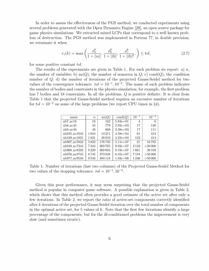
In order to assess the effectiveness of the PGS method, we conducted experiments usingseveral problems generated with the Open Dynamics Engine [29], an open source package forgame physics simulations. We extracted mixed LCPs that correspond to a well known prob-lem of destruction. The PGS method was implemented in Fortran 77, in double precision;we terminate it when

r1(k) = max

(

ρka

1 + ||a||,

ρkb

1 + ||b||,

ρkc

1 + ||b||2,

)

≤ tol, (2.7)

for some positive constant tol.The results of the experiments are given in Table 1. For each problem we report: a) n,

the number of variables; b) nz(Q), the number of nonzeros in Q; c) cond(Q), the conditionnumber of Q; d) the number of iterations of the projected Gauss-Seidel method for twovalues of the convergence tolerance: tol = 10−1, 10−2. The name of each problem indicatesthe number of bodies and constraints in the physics simulation; for example, the first problemhas 7 bodies and 18 constraints. In all the problems, Q is positive definite. It is clear fromTable 1 that the projected Gauss-Seidel method requires an excessive number of iterationsfor tol = 10−2 on some of the large problems (we report CPU times in §4).

name n nz(Q) cond(Q) 10−1 10−2

nb7 nc18 18 162 5.83e+01 4 6nb8 nc45 45 779 2.92e+03 17 120nb8 nc48 48 868 2.38e+03 17 111nb235 nc1044 1 044 14 211 4.58e+04 61 312nb449 nc1821 1 821 28 010 4.22e+04 132 414nb907 nc5832 5 832 176 735 5.11e+07 21 16 785nb948 nc7344 7 344 269 765 9.02e+07 3 123 >50 000nb966 nc8220 8 220 368 604 9.19e+07 1 601 39 103nb976 nc8745 8 745 373 848 6.45e+07 7 184 >50 000nb977 nc9534 9 534 494 118 1.03e+08 1 246 >50 000

Table 1: Number of iterations (last two columns) of the Projected Gauss-Seidel Method fortwo values of the stopping tolerance: tol = 10−1, 10−2.

Given this poor performance, it may seem surprising that the projected Gauss-Seidelmethod is popular in computer game software. A possible explanation is given in Table 2,which shows that this method often provides a good estimate of the active set after only afew iterations. In Table 2, we report the ratio of active-set components correctly identifiedafter k iterations of the projected Gauss-Seidel iteration over the total number of componentsin the optimal active set, for 5 values of k. Note that the first few iterations identify a largepercentage of the components, but for the ill-conditioned problems the improvement is veryslow (and sometimes erratic).

6

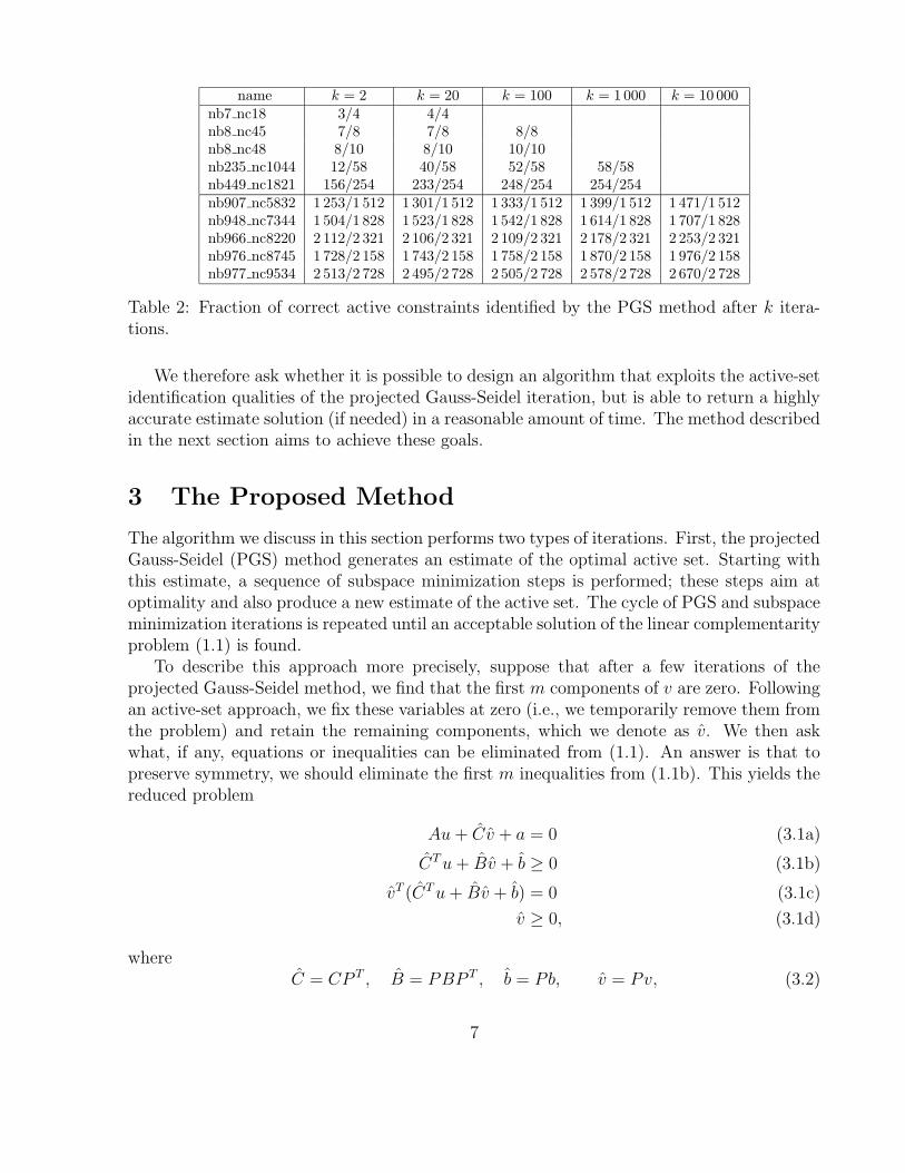
name k = 2 k = 20 k = 100 k = 1000 k = 10 000nb7 nc18 3/4 4/4nb8 nc45 7/8 7/8 8/8nb8 nc48 8/10 8/10 10/10nb235 nc1044 12/58 40/58 52/58 58/58nb449 nc1821 156/254 233/254 248/254 254/254nb907 nc5832 1 253/1 512 1 301/1 512 1 333/1 512 1 399/1 512 1 471/1 512nb948 nc7344 1 504/1 828 1 523/1 828 1 542/1 828 1 614/1 828 1 707/1 828nb966 nc8220 2 112/2 321 2 106/2 321 2 109/2 321 2 178/2 321 2 253/2 321nb976 nc8745 1 728/2 158 1 743/2 158 1 758/2 158 1 870/2 158 1 976/2 158nb977 nc9534 2 513/2 728 2 495/2 728 2 505/2 728 2 578/2 728 2 670/2 728

Table 2: Fraction of correct active constraints identified by the PGS method after k itera-tions.

We therefore ask whether it is possible to design an algorithm that exploits the active-setidentification qualities of the projected Gauss-Seidel iteration, but is able to return a highlyaccurate estimate solution (if needed) in a reasonable amount of time. The method describedin the next section aims to achieve these goals.

3 The Proposed Method

The algorithm we discuss in this section performs two types of iterations. First, the projectedGauss-Seidel (PGS) method generates an estimate of the optimal active set. Starting withthis estimate, a sequence of subspace minimization steps is performed; these steps aim atoptimality and also produce a new estimate of the active set. The cycle of PGS and subspaceminimization iterations is repeated until an acceptable solution of the linear complementarityproblem (1.1) is found.

To describe this approach more precisely, suppose that after a few iterations of theprojected Gauss-Seidel method, we find that the first m components of v are zero. Followingan active-set approach, we fix these variables at zero (i.e., we temporarily remove them fromthe problem) and retain the remaining components, which we denote as v. We then askwhat, if any, equations or inequalities can be eliminated from (1.1). An answer is that topreserve symmetry, we should eliminate the first m inequalities from (1.1b). This yields thereduced problem

Au + Cv + a = 0 (3.1a)

CT u + Bv + b ≥ 0 (3.1b)

vT (CT u + Bv + b) = 0 (3.1c)

v ≥ 0, (3.1d)

whereC = CP T , B = PBP T , b = Pb, v = Pv, (3.2)

7

and P = [ 0 | Inb−m]. Since the active set approach has v > 0, we set the term CT u + Bv + b

in (3.1c) to zero. Thus (3.1) reduces to the square system

Au + Cv + a = 0 (3.3a)

CT u + Bv + b = 0, (3.3b)

together with the condition v ≥ 0. We compute an approximate solution of this problem bysolving (3.3) and then projecting the solution v onto the nonnegative orthant through theassignment

v ← max(0, v). (3.4)

The components of v that are set to zero by the projection operation (3.4) are then removedto obtain a new subspace minimization problem of smaller dimension. The correspondingreduced system (3.3) is formed and solved. We repeat this subspace minimization procedureuntil the solution of (3.3) contains no negative components in v or until a prescribed max-imum number of subspace iterations is performed. In either case the procedure terminateswith a point that we denote as zs = (us, vs). (Here and in what follows, z denotes a vectorin R

n where the componenent v is obtained from the reduced vector v by appending anappropriate number of zeros to it.)

One extra ingredient is added in the algorithm to guarantee global convergence (in thepositive definite case). We compute a safeguarding point zb by backtracking (instead ofprojecting) from the first subspace solution to the feasible region v ≥ 0. More precisely, wecompute

zb = z0 + α(z1 − z0), (3.5)

where z0 is the initial point in the subspace minimization phase, z1 is the point obtainedby solving the system (3.3) for the first time (and before applying the projection (3.4)),and 0 < α ≤ 1 is the largest steplength such that vb ≥ 0. We store zb and perform therepeated subspace minimization phase described above to obtain the point zs. We thenchoose between zb and zs, depending on which one is preferable by some metric, such as theoptimality measure (2.6).

However, in the case when Q is positive definite, it is natural to use the quadratic functionφ given in (1.4) as the metric. Recall from §1, that the linear complementarity problem (1.1)and the bound constrained quadratic program (1.4) are equivalent when Q is positive definite.It is easy to explain the utility of the point zb by interpreting the solution of (3.3)-(3.4) inthe context of this quadratic program. Suppose, once more, that we have removed the firstm components of v and that v are the remaining components. We then define the reducedquadratic program

minz

φ(z) =1

2zT Qz + qT z

s.t. v ≥ 0,(3.6)

where z = (u, v) and Q, q are defined accordingly by means of the matrix P . The uncon-strained minimizer of the objective in (3.6) coincides with the solution of (3.3), which justifies

8

the use of the term “subspace minimization” in our earlier discussion. Note, however, thatby projecting the solution of (3.3) through (3.4) the value of the quadratic function φ maybe higher than at the initial point z0 of the subspace minimization, which can cause thealgorithm to fail. This difficulty is easily avoided by falling back on the point zb, which isguaranteed to give φ(zb) ≤ φ(z0). In this way, we ensure that the subspace minimizationdoes not undo the progress made in the PGS phase. In this case we replace zs by zb ifφ(zb) < φ(zs).

The proposed algorithm is summarized as follows for the case when Q is positive definite.

Algorithm 3.1 Projected Gauss-Seidel with Subspace Minimization

Initialize u, v ≥ 0. Choose a constant tol > 0.repeat until a convergence test for problem (1.1) is satisfied

Perform kgs iterations of the projected Gauss-Seidel iteration (see Algorithm 2.1)to obtain an iterate z0 = (u, v);Set isub← 1;repeat at most ksm times (subspace minimization)

Define v to be the subvector of v whose components satisfy vi > tol;Form and solve the reduced system (3.3) to obtain z1;if isub = 1 compute zb by (3.5);Project the solution of (3.3) by means of (3.4);Denote the new iterate of the subspace minimization by zs = (us, vs);If the solution component v satisfies v > tol, break;Set isub← 0;

end repeatIf φ(zs) > φ(zb) then set zs ← zb;Define the new iterate of the algorithm as z = (u, v)← zs

end repeat

Practical ranges for the parameters are kgs ∈ [2, 5] and ksm ∈ [3, 5]. We could replacethe projected Gauss-Seidel iteration by the projected SOR iteration [13], but even when theSOR parameter is tuned to the application, we can expect only a marginal improvement ofperformance, for the reasons discussed below.

The algorithm of Kocvara and Zowe [19] is a special case of Algorithm 3.1 where onlyone subspace minimization step is performed, i.e., ksm = 1. Another important differenceis that Kocvara and Zowe always use the backtracking procedure (3.5), instead of firsttrying the projection point (3.4), which is often much more effective in the identification ofthe optimal active set. The refinements introduced in our algorithm are crucial; withoutthem the method can be very inefficient on ill-conditioned problems (as we report in §4).Kocvara and Zowe observed these inefficiencies and attempt to overcome them by devisinga procedure for computing a good initial point and employing certain heuristics in the linesearch procedure.

9

The subspace minimization could be performed using a procedure that guarantees asteady decrease in φ. For example, Lin and More [21] perform an approximate minimizationof φ along the path generated by projecting the subspace minimization point z1 onto thenonnegative orthant v ≥ 0. Their procedure can produce a better iterate than the subspaceminimization of Algorithm 3.1, but our nonmonotone approach has the advantage that theprojection (3.4) can improve the active set estimate very quickly and that the computationalcost of the iteration can easily be controlled through the parameter ksm. In our tests, itwas never necessary for Algorithm 3.1 to revert to the safeguarding point zb defined in(3.5), despite the fact that, on occasion, φ increased after the first step of the subspaceminimization. Thus, our approach is indeed nonmonotone.

Algorithm 3.1 is well defined even if Q is not positive definite; all we need to assume isthat the diagonal elements of B are positive and the diagonal elements of A are nonzero. Thefunction φ would then be defined as the optimality measure of the problem, as mentionedabove. However, when Q is not positive definite the global convergence of the algorithmcannot be guaranteed.

4 Numerical experiments

We first compare three methods that work directly on the mixed linear complementarityproblem: the projected Gauss-Seidel method (Algorithm 2.1), the method proposed in thispaper (Algorithm 3.1) and an interior-point method.

The interior-point method is a primal-dual algorithm for LCPs applied to the system(1.3). We use separate steplengths for the variables v and w. The centering parameter is setto σ = 0.25 throughout the iteration and the fraction to the boundary parameter is definedas τ = 0.9995; see Wright [31] for a description of the algorithm and the meaning of theseparameters. The stopping condition for the interior-point method is defined in terms of theresiduals

rka = Auk + Cvk + a, rk

b = CT uk + Bvk − wk + b, rkc = V kwk, (4.1)

where V is a diagonal matrix whose nonzero entries are given by the components of v.In order to make the numerical comparisons as accurate as possible, we have implemented

these three methods in a Fortran 77 package (using double precision), and employ the samelinear algebra solver, namely pardiso [26, 27], to solve the linear systems arising in Algo-rithms 3.1 and the interior-point method. The latter performs the symbolic factorizationonly once, whereas Algorithm 3.1 does so at every subspace iteration. The package was com-piled using GNU f77 and all computations were performed on a Pentium 4 Dell Precision

340.In our implementation of Algorithm 3.1, we performed kgs = 5 PGS iterations before

invoking the subspace minimization phase, which was repeated at most ksm = 3 times. Theinitial point in Algorithm 3.1 and the PGS method was chosen as u0 = 0, v0 = 0, and for theinterior-point method it was set to u0 = 0, v0 = 0.1, w0 = 1. To terminate the interior-point

10

method, we define the error

r2(k) = max

(

||rka||

1 + ||a||,||rk

b ||

1 + ||b||,||rk

c ||

1 + ||b||2,

)

(4.2)

where ra, rb, rc are given in (4.1). For the PGS method and Algorithm 3.1 we use the errormeasure (2.7). In the first set of experiments, the algorithms were terminated when r1(k)and r2(k) were less than 10−8.

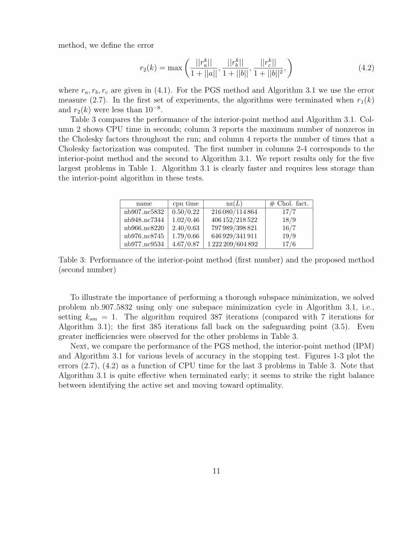
Table 3 compares the performance of the interior-point method and Algorithm 3.1. Col-umn 2 shows CPU time in seconds; column 3 reports the maximum number of nonzeros inthe Cholesky factors throughout the run; and column 4 reports the number of times that aCholesky factorization was computed. The first number in columns 2-4 corresponds to theinterior-point method and the second to Algorithm 3.1. We report results only for the fivelargest problems in Table 1. Algorithm 3.1 is clearly faster and requires less storage thanthe interior-point algorithm in these tests.

name cpu time nz(L) # Chol. fact.nb907 nc5832 0.50/0.22 216 080/114 864 17/7nb948 nc7344 1.02/0.46 406 152/218 522 18/9nb966 nc8220 2.40/0.63 797 989/398 821 16/7nb976 nc8745 1.79/0.66 646 929/341 911 19/9nb977 nc9534 4.67/0.87 1 222 209/604 892 17/6

Table 3: Performance of the interior-point method (first number) and the proposed method(second number)

To illustrate the importance of performing a thorough subspace minimization, we solvedproblem nb 907 5832 using only one subspace minimization cycle in Algorithm 3.1, i.e.,setting ksm = 1. The algorithm required 387 iterations (compared with 7 iterations forAlgorithm 3.1); the first 385 iterations fall back on the safeguarding point (3.5). Evengreater inefficiencies were observed for the other problems in Table 3.

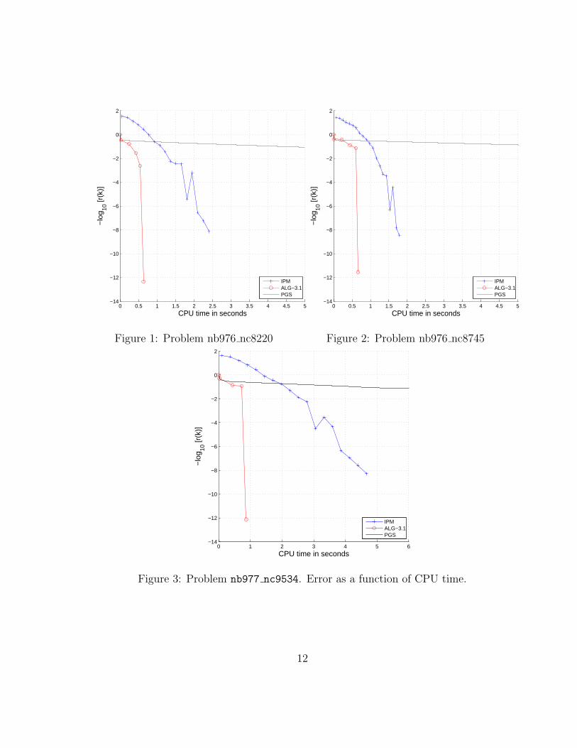
Next, we compare the performance of the PGS method, the interior-point method (IPM)and Algorithm 3.1 for various levels of accuracy in the stopping test. Figures 1-3 plot theerrors (2.7), (4.2) as a function of CPU time for the last 3 problems in Table 3. Note thatAlgorithm 3.1 is quite effective when terminated early; it seems to strike the right balancebetween identifying the active set and moving toward optimality.

11

0 0.5 1 1.5 2 2.5 3 3.5 4 4.5 5−14

−12

−10

−8

−6

−4

−2

0

2

CPU time in seconds

−lo

g 10 [r

(k)]

IPMALG−3.1PGS

Figure 1: Problem nb976 nc8220

0 0.5 1 1.5 2 2.5 3 3.5 4 4.5 5−14

−12

−10

−8

−6

−4

−2

0

2

CPU time in seconds−

log 10

[r(k

)]

IPMALG−3.1PGS

Figure 2: Problem nb976 nc8745

0 1 2 3 4 5 6−14

−12

−10

−8

−6

−4

−2

0

2

CPU time in seconds

−lo

g 10 [r

(k)]

IPMALG−3.1PGS

Figure 3: Problem nb977 nc9534. Error as a function of CPU time.

12

In a second set of experiments, we compare Algorithm 3.1 and the PGS method to agradient projection method. Since Q is positive definite for all the problems in Table 1, wecan solve the LCP by applying the gradient projection method to the quadratic program(1.4). A great variety of gradient projection methods have been developed in the last 20years; some variants [6, 7, 5, 14, 18] perform only gradient projection steps, while others[24, 10, 23, 32, 21] alternate gradient projection and subspace minimization steps.

For our tests we have chosen tron, a well established code by Lin and More [21] thathas been tested against other gradient projection methods [18, 5]. The algorithm in tron

alternates one gradient projection step and a (repeated) subspace minimization phase, whichis performed using a conjugate gradient iteration preconditioned by a (modified) incompleteCholesky factorization.

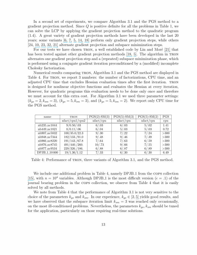
Numerical results comparing tron, Algorithm 3.1 and the PGS method are displayed inTable 4. For tron, we report 3 numbers: the number of factorizations, CPU time, and anadjusted CPU time that excludes Hessian evaluation times after the first iteration. tron

is designed for nonlinear objective functions and evaluates the Hessian at every iteration,However, for quadratic programs this evaluation needs to be done only once and thereforewe must account for this extra cost. For Algorithm 3.1 we used three parameter settings:(kgs = 2, ksm = 3), (kgs = 5, ksm = 3), and (kgs = 5, ksm = 2). We report only CPU time forthe PGS method.

name tron PGS(2)-SM(3) PGS(5)-SM(3) PGS(5)-SM(2) PGSnfact/cpu1/cpu2 nfact/cpu nfact/cpu nfact/cpu cpu

nb235 nc1044 9/0.50/.03 6/.03 6/.03 5/.02 1.41nb449 nc1821 8/0.11/.06 6/.04 5/.03 5/.03 0.72nb907 nc5832 100/35.0/22.3 9/.30 7/.22 7/.24 >300nb948 nc7344 182/133./91.0 9/.48 9/.46 7/.39 >300nb966 nc8220 191/143./67.8 7/.64 7/.63 6/.59 >300nb976 nc8745 491/440./260. 10/.73 9/.66 7/.55 >300nb977 nc9534 229/326./186. 6/.88 6/.87 6/.89 >300DPJB 1 10 000 19/1.36/1.12 7/.33 6/.30 6/.30 6.49

Table 4: Performance of tron, three variants of Algorithm 3.1, and the PGS method.

We include one additional problem in Table 4, namely DPJB 1 from the cops collection[15], with n = 104 variables. Although DPJB 1 is the most difficult version (ε = .1) of thejournal bearing problem in the cops collection, we observe from Table 4 that it is easilysolved by all methods.

We note from Table 4 that the performance of Algorithm 3.1 is not very sensitive to thechoice of the parameters kgs and ksm. In our experience, kgs ∈ [2, 5] yields good results, andwe have observed that the subspace iteration limit ksm = 3 was reached only occasionally,on the most ill-conditioned problems. Nevertheless, the parameters kgs, ksm should be tunedfor the application, particularly on those requiring real-time solutions.

13

These results also indicate that little would be gained by replacing the projected Gauss-Seidel iteration by the projected SOR iteration, given that we have found it best to performat most 5 iterations of the projected iterative method. Since the Gauss-Seidel method doesnot require the selection of parameters, we find it preferable to the SOR method.

Note that tron requires a very large number of iterations for the ill-conditioned problems(i.e. the last 5 problems in Table 1) and requires significantly more time than Algorithm 3.1.This is due to the fact that the subspace minimization in tron is not able to produce anaccurate estimate of the active set and, in addition, that it requires between 4 and 10 timesmore CPU time than the subspace minimization in Algorithm 3.1.

We have not made comparisons with the algorithm of Kocvara and Zowe because theirnumerical results report only moderate improvements in performance over the gradient pro-jection method gpcg [23]) that does not employ preconditioning. Our results, on the otherhand, show dramatic improvements over the more powerful gradient projection code tron

which uses an incomplete Cholesky preconditioner.

5 Final Remarks

In this paper we have proposed an algorithm for solving symmetric mixed linear comple-mentarity problems (and as a special case, convex bound constrained quadratic programs)that places emphasis on the speed and accuracy of the subspace minimization phase. Thealgorithm is designed for medium to large real-time applications and our tests suggest thatit has far better performance on ill-conditioned problems than competing methods. Theproposed algorithm has much flexibility since the number of projected Gauss-Seidel andsubspace minimization iterations can be adapted to the requirements of the application athand.

Another advantage of the proposed method is that it can exploit parallelism well. Theprojected Gauss-Seidel method, which is popular in computer game software and Americanoptions pricing, scales poorly with the number of processors due to dependencies betweenthe equations. For example, Kumar et al. simulated the performance of a PGS step on a64-core Intel chip multiprocessor simulator and observed less than 15% utilization [20]. Onthe other hand, Algorithm 3.1 typically spends only 10% of the time in the PGS phase and90% in the subspace minimization. Hence it effectively offloads the parallelization task toa direct linear solver that is known to parallelize well [28]. Specifically, our adaptation ofpardiso, the Cholesky solver used for the experiments in this paper, yields more than 65%utilization on a 64-core chip multiprocessor simulator (see also Schenk [25] for a scalabilitystudy for a moderate number of processors on a coarsely coupled shared memory system).

There has been a recent emergence of accelerated physics solutions in the computerindustry. Ageia has developed a stand-alone physics processing unit [1], while graphicsprocessing unit makers ATI and Nvidia have introduced new physics engines that run ontheir chips [2]. These approaches use massively parallel architectures that can benefit fromthe features of Algorithm 3.1. In future work, we intend to perform further quantitativestudies of Algorithm 3.1 on various emerging chip multiprocessors.

14

References

[1] Ageia physx. Web page, http://www.ageia.com/ physx/ , 2006.

[2] HavokFX. Web page, http://www.havok.com/ content/view/187/77/ , 2006.

[3] M. Anitescu and F. A. Potra. Formulating dynamic multi-rigid-body contact problemswith friction as solvable linear complementarity problems. Nonlinear Dynamics, 14::231–247, 1997.

[4] D. P. Bertsekas. Projected Newton methods for optimization problems with simpleconstraints. SIAM Journal on Control and Optimization, 20(2):221–246, 1982.

[5] E G. Birgin and J. M. Martınez. Large-scale active-set box-constrained optimizationmethod with spectral projected gradients. Comput. Optim. Appl., 23:101—125, 2002.

[6] E G. Birgin, J. M. Martınez, and M. Raydan. Nonmonotone spectral projected gradientmethods on convex sets. SIOPT, 10:1196—1211, 2000.

[7] E G. Birgin, J. M. Martınez, and M. Raydan. Algorithm 813: Spg–software for convex-constrained optimization. ACM Trans. Math. Software, 27:340—349, 2001.

[8] J. V. Burke and J. J. More. On the identification of active constraints. SIAM Journalon Numerical Analysis, 25(5):1197–1211, 1988.

[9] E. Catto. Iterative dynamics with temporal coherence. Technical report, Crystal Dy-namics, Menlo Park, California, 2005.

[10] A. R. Conn, N. I. M. Gould, and Ph. L. Toint. Global convergence of a class of trustregion algorithms for optimization with simple bounds. SIAM Journal on NumericalAnalysis, 25(182):433–460, 1988. See also same journal 26:764–767, 1989.

[11] A. R. Conn, N. I. M. Gould, and Ph. L. Toint. LANCELOT: a Fortran package for Large-scale Nonlinear Optimization (Release A). Springer Series in Computational Mathemat-ics. Springer Verlag, Heidelberg, Berlin, New York, 1992.

[12] R.W. Cottle and G.B. Dantzig. Complementarity pivot theory of mathematical pro-gramming. J. Linear Algebra Applns., 1:103–125, 1968.

[13] R.W. Cottle, J-S Pang, and R. E. Stone. The Linear Complementarity Problem. Aca-demic Press, 1992.

[14] Y. H. Dai and R. Fletcher. Projected Barzilai-Borwein methods for large-scale box-constrained quadratic programming. Numer. Math., 100, 2005.

[15] E. D. Dolan, J. J. More, and T. S. Munson. Benchmarking optimization softwarewith COPS 3.0. Technical Report ANL/MCS-TM-273, Argonne National Laboratory,Argonne, Illinois, USA, 2004.

15

[16] M. C. Ferris and J. S. Pang. Engineering and economic applications of complementarityproblems. SIAM Review, 39(4):669–713, 1997.

[17] M.C. Ferris, A.J. Wathen, and P. Armand. Limited memory solution of bound con-strained convex quadratic problems arising in video games. RAIRO- Operations Re-search, 41:19–34, 2007.

[18] W. W. Hager and H. Zhang. A new active set algorithm for box constrained optimiza-tion. SIOPT, 17(2):526–557, 2007.

[19] M. Kocvara and J. Zowe. An iterative two-step algorithm for linear complementarityproblems. Numerische Mathematik, 68:95–106, 1994.

[20] S. Kumar, C. J. Hughes, and A. Nguyen. Carbon: Architectural support for fine-grained parallelism on chip multiprocessors. In Proceedings of IEEE/ACM InternationalSymposium on Computer Architecture (ISCA), San Diego, California, 2007.

[21] C. J. Lin and J. J. More. Newton’s method for large bound-constrained optimizationproblems. SIAM Journal on Optimization, 9(4):1100–1127, 1999.

[22] J.L Morales and R.W.H. Sargent. Computational experience with several methodsfor large-scale convex quadratic programming. Aportaciones Matematicas. Comunica-ciones, 14:141–158, 1994.

[23] J. J. More and G. Toraldo. On the solution of large quadratic programming problemswith bound constraints. SIAM Journal on Optimization, 1(1):93–113, 1991.

[24] D. P. O’Leary. A generalized conjugate gradient algorithm for solving a class of quadraticprogramming problems. Linear Algebra and its Applications, 34:371–399, 1980.

[25] O. Schenk. Scalable parallel sparse LU factorization methods on shared memory multi-processors. PhD thesis, Swiss Federal Institute of Technology, Zurich, 2000.

[26] O. Schenk and K. Gartner. Solving unsymmetric sparse systems of linear equationswith pardiso. Journal of Future Generation Computer Systems, 20(3):475–487, 2004.

[27] O. Schenk and K. Gartner. On fast factorization pivoting methods for symmetric in-definite systems. Elec. Trans. Numer. Anal., 23:158–179, 2006.

[28] M. Smelyanskiy, V. W. Lee, D. Kim, A. D. Nguyen, and P. Dubey. Scaling perfor-mance of interior-point methods on a large-scale chip multiprocessor system. In SC ’07:Proceedings of the 2007 ACM/IEEE conference on Supercomputing, 2007.

[29] R. Smith. Open dynamics engine. Technical report, 2004. http://www.ode.org.

[30] P. Wilmott. Quantitative Finance. J. Wiley and sons, 2006.

16

[31] S. J. Wright. Primal-Dual Interior-Point Methods. SIAM, Philadelphia, USA, 1997.

[32] C. Zhu, R. H. Byrd, P. Lu, and J. Nocedal. Algorithm 78: L-BFGS-B: Fortran subrou-tines for large-scale bound constrained optimization. ACM Transactions on Mathemat-ical Software, 23(4):550–560, 1997.

17