Complementarity Models for Traffic Equilibrium with Ridesharing

Complementarity Models for Traffic Equilibrium with Ridesharing

Huayu Xu∗, Jong-Shi Pang†, Fernando Ordonez‡, and Maged Dessouky§

Original April 2015; revised July 2015; final August 2015

Abstract

It is estimated that 76% of commuters are driving to work alone while each of them experiencesa 38-hour delay annually due to traffic congestion. Ridesharing is an efficient way to utilize theunused capacity and help with congestion reduction, and it has recently become more and morepopular due to new communication technologies. Understanding the complex relations betweenridesharing and traffic congestion is a critical step in the evaluation of a ridesharing enterpriseor of the effectiveness of regulatory policies or incentives to promote ridesharing. The objectiveof this paper is to introduce a mathematical framework for the study of the ridesharing impactson traffic congestion and to pave the way for the analysis of how people can be motivated toparticipate in ridesharing, and conversely, how congestion influences ridesharing activities. Weaccomplish this objective by developing a new traffic equilibrium model with ridesharing, andformulating the model as a mixed complementarity problem (MiCP). We provide conditionson the model parameters under which there exists one and only one solution to this model.The computational results show that when the congestion cost decreases or the ridesharinginconvenience cost increases, more travelers would become solo drivers and thus less peoplewould participate in ridesharing. On the other hand, when the ridesharing price increases, moretravelers would become ridesharing drivers.

1 Introduction

For many years traffic congestion has been a significant transportation problem, especially in largeurban areas, and congestion reduction has been a hot but tough issue in both academic research andcity planning. According to The 2012 Annual Urban Mobility Report [?], it is estimated that (a)the average annual delay endured by each commuter was 38 hours (compared to 16 hours in 1982),and (b) the annual cost of congestion is more than $120 billion–nearly $820 for every commuterin the United States. The expansion speed of the population of commuters is always one stepahead of the infrastructure capacity. At the same time, according to the Transportation StatisticsAnnual Report 2012 by the Bureau of Transportation Statistics [?], 76.4% of commuters drove to

∗The Daniel J. Epstein Department of Industrial and Systems Engineering, University of Southern California, LosAngeles, California 90089-0193 U.S.A. Email:[email protected].†The Daniel J. Epstein Department of Industrial and Systems Engineering, University of Southern California, Los

Angeles, California 90089-0193, U.S.A. The work of this author was based on research supported by the U.S. Nationalscience Foundation under grant CMMI-1402052. Email: [email protected].‡Industrial Engineering Department, Universidad de Chile, Republica 701, Santiago, Chile. Email:

[email protected].§Corresponding author. The Daniel J. Epstein Department of Industrial and Systems Engineering, University of

Southern California, Los Angeles, California 90089-0193 U.S.A. The research of this author was supported by theFederal Highway Administration under the Broad Agency Announcement of Exploratory Advanced Research. Email:[email protected].

1

work alone in 2011. Therefore there exists an urgent need to tap into such a significant amount ofunused capacity in transportation networks.

Ridesharing, or carpooling, appears as one such innovative transportation mode that could helpfulfill such a need and also mitigate the congestion increase. Benefits of ridesharing include travelcost savings, reducing travel time, mitigating traffic congestion, conserving fuel, and reducing airpollution [?, ?, ?, ?]. Recently, technological advances including global positioning systems (GPS)and mobile devices have greatly enhanced the communication capabilities of travelers, facilitatingthe creation of ridesharing in real-time. Taking advantage of this opportunity, a number of com-panies, such as Uber, Lyft, Avego (Carma), SideCar, etc., have emerged to develop systems wheretravelers (including both drivers and passengers) can be matched in real time via mobile apps [?].In a sense these companies are establishing a marketplace for drivers to offer up their empty seats toother travelers. The essential difference of such ridesharing systems from traditional public transitsystems is that they do not hire professional drivers and they function as a matching agency thatpairs passengers with “citizen” drivers.

In a previous paper [?], we studied a transportation system where ridesharing has the ability ofcapturing a significant portion of travel demand via a real-time matching agency. In this ridesharingsystem, we assume that the passengers will pay the drivers for the ridesharing services to sharethe travel cost. The ridesharing price is an abstraction to represent compensation that driverstake into account in their decision to participate in ridesharing, such as a reduction in travel timeor toll costs that will occur by being able to use high-occupancy vehicle (HOV) lanes. We alsoassume that the system operates as an open marketplace and thus the ridesharing price will bedetermined by the market, e.g. the drivers and passengers that are participating in ridesharing.In our previous paper, for simplicity we assumed that drivers and passengers who share the samevehicle must be traveling from the same origin to the same destination. In this paper, we focus onrelaxing this assumption to develop a more general and representative mode of ridesharing. As isin most realistic ridesharing scenarios, drivers may make a detour, slight or big, to pick up or dropoff some passenger(s).

The purpose of this paper is to determine how people will behave where there exists such a rideshar-ing market, and furthermore determine how ridesharing activities would impact the traffic conges-tion. The travelers are categorized in three types: (a) solo drivers who drive alone, (b) ridesharingdrivers who share their car, and (c) passengers who take a ride. The major decision factors for thetravelers to choose their traveling types include the traffic congestion, the ridesharing price and theinconvenience caused by ridesharing activities. For instance, to decide whether to participate inridesharing, drivers may weigh the inconvenience, such as loss of privacy, against the compensationthey may earn for taking on passengers. In turn, passengers would tradeoff the inconvenience, suchas security concerns and loss of freedom, against the travel time and cost of a shared ride. Thesetradeoffs would balance in an equilibrium that determines the traffic congestion, the ridesharingprices, and the number of different types travelers. For example, an increase in ridesharing (morepassengers) could lead to a reduction in congestion, which in turn makes it less stressful to be adriver, leading to an increase in drivers and thus an increase in congestion. Understanding howridesharing would influence traffic congestion is fundamental in the evaluation of a ridesharing en-terprise or in assessing the effectiveness of regulatory policies or incentives to promote ridesharing.

Obviously, a ridesharing system, due to the individual roles of the three types of travelers, is distinctfrom a multi-modal transportation system wherein passengers can select multiple modes of travelon a trip, but the modes selected do not influence the capacity or cost of alternative modes of

2

travel. In a ridesharing system, a driver can decide to pick up passengers, which influences theavailability and costs of shared rides.

However, we do not include a detailed assignment of passengers to vehicles. We are only modelingthe behavior of the aggregate quantities of drivers and passengers. In the proposed model thereonly exist ridesharing passengers on an arc (road segment) if there are ridesharing drivers traversingthe corresponding arc. A certain passenger can be taken only if there is enough capacity on thecorresponding ridesharing vehicles. If there are none, then the traveler has the options to be a solodriver or ridesharing driver and would select the one that is less expensive.

The paper is organized as follows. Section 2 presents a literature review, including both ridesharingsystems and traffic assignment problems. Section 3 models our ridesharing system as a mixedcomplementarity problem and Section 4 presents the computational results and analysis. We finishthe paper with conclusions in Section 5.

2 Literature Review

Ridesharing is a joint-trip of at least two participants that share a vehicle and requires coordinationwith respect to itineraries [?]. Some ridesharing services occur spontaneously among individualtravelers motivated by access to faster HOV (High-Occupancy Vehicle) lanes or reduced tolls.Examples of this type of ridesharing service are casual carpooling [?, ?], and slugging, whichformed in the Washington D.C. area free of charge to the participants [?, ?]. These services run ontheir own momentum; they are not started or run by a public or private entity [?]. Therefore theyare limited to specific locations or circumstances and are difficult to replicate elsewhere.

With innovative technologies inhibitors of ridesharing can be overcome and a number of privatematching agencies have emerged during the last decade [?, ?, ?, ?, ?]. Such ridesharing servicesare operated by agencies that provide ride-matching opportunities for participants without regardto any previous historical involvement [?]. By introducing mobile technologies like smart phones aswell as global positioning systems (GPS), ridesharing systems can be implemented in real-time. Thisallows matching agencies to incorporate current locations and travel itineraries in better proposalsto travelers, which could lead to increasing the degree of adoption of ridesharing systems.

However, the literature discussing the relationship or the interaction between ridesharing activitiesand traffic congestion is quite limited. The paper [?] discussed the carpooling behavior and theoptimal congestion pricing in a multilane highway with or without HOV lanes where the first-best pricing and the second-best pricing models were formulated and compared. The models,however, were limited to identical commuters (single origin and single destination, SOSD) and thenumber of passengers in each carpooling vehicle is fixed to one. The paper [?] studied the morningcommute problem with three modes: transit, driving alone and carpool. The authors analyzed theinteractions among the three modes and how different factors affect their mode shares and networkperformance. Again, the model is limited to a SOSD network and does not consider the interactionsof ridesharing between different origin-destination (OD) pairs.

To study the effects of multiple OD pairs, one classic model is the traffic assignment problem (TAP)[?], which evaluates the distribution of travelers among different routes and OD pairs. The basicassumption underlying this problem is the renowned Wardop’s user equilibrium principle [?] whichpostulates that the travel times (congestion costs) in all the used paths are equal and not more thanthose that would be experienced by a vehicle on any unused path. Mathematically, this principle isthe cornerstone to the complementarity and variational inequality approach of the user equilibrium

3

(UE) problem pioneered by Aashitiani and Magnanti [?] and Dafermos [?]; see [?, Section 1.4.5] fordetails of this approach and the Notes and Comments Section 1.9 for a historical account and morereferences on this problem. Recent references include [?, ?, ?, ?] as well as some recent work onthe continuous-time versions of the dynamic UE mentioned before. In [?], an optimization modelwas introduced for the ridesharing traffic assignment problem under the assumption of no detoursfor passenger pick up and drop off. When the latter assumption is removed, the optimizationframework is no longer applicable and we need to resort to a variational inequality (VI) or itsequivalent complementarity formulation. The cited paper also treats the case of elastic demandsby introducing a utility for travel; the problem decides not only how people will choose their paths,but also how many people would travel given certain congestion conditions. This kind of modelserves to illustrate those cases where people might not travel when the traffic is highly congested.While the VI approach can treat elastic demands in the ridesharing framework, we will focus onthe fixed-demand ridesharing model in this paper.

3 Mathematical Model

The ridesharing equilibrium problem with multiple OD pairs is not amenable to solution as anoptimization problem because it lacks an obvious objective function. Instead, we formulate theproblem as a mixed complementarity problem. This allows us to determine the type (solo driver,ridesharing driver, or passenger) a traveler chooses to be and to understand the relations betweenridesharing activities and traffic congestion when such conditions change.

Our roadmap to the analysis of a ridesharing user equilibrium is as follows. We first introduce anexpanded network to model the ridesharing paradigm; this is followed by a formal definition of aridesharing user equilibrium and its natural formulation as a mixed complementarity problem (interms of path flows) whose solution is shown to yield such an equilibrium. Next, it is shown thatthe arc flows induced by such equilibrium path flows must be a solution to a variational inequality(VI). We show that the latter VI has a unique solution under a set of mild conditions on themodel constants. The upshot of this uniqueness result is that while the path flows of a ridesharinguser equilibrium are not necessarily unique, under some mild conditions, there is a unique set ofarc flows induced by any such (path-flow) equilibrium. This uniqueness conclusion extends to theridesharing case a known result of traffic equilibrium. Some numerical examples are presented toillustrate the overall approach.

Consider a transportation network represented by a graph with nodes and arcs, where nodes couldbe origins, destinations or intermediate stops, and arcs are direct roads that connect two nodes.Each individual travels from an origin to a destination, which is called an origin-destination (OD)pair. For each OD pair, there exist multiple paths that start from the origin and end at the destina-tion. Travelers are categorized into three groups: solo drivers, ridesharing drivers and passengers.They experience different costs due to different paths and different roles. More specifically, weassume that:

• There are three traveler roles: solo drivers, ridesharing drivers and passengers.

• Drivers may pick up or drop off any passenger(s) at any time anywhere. That is tosay, drivers and passengers who are sharing the same vehicle may or may not travel on the sameOD pair. Drivers may even detour for a passenger if needed.

• All drivers must be driving throughout their trips. Solo drivers and ridesharing driversmay switch roles (when picking up or dropping off passengers in the middle of their trips), but

4

neither can become a passenger.

• All passengers must remain passengers throughout their trips. They cannot become adriver in the middle of trips once they have decided to travel as a passenger.

• The total number of travelers of each OD pair is fixed. However, for each traveler, theymay decide to be a solo driver, a ridesharing driver or a passenger.

• The vehicle capacity is limited and fixed for all ridesharing vehicles. In other words,the number of passengers in each vehicle cannot exceed a given limit.

We note that since travelers experience different costs due to different paths and different roles,travelers could face different costs even on the same path. Therefore travelers select the path androle that give them the least cost, impacting other travelers’ costs, until an equilibrium is reached.Given the above assumptions, our goal is to derive a model that determines how travelers willchoose their roles and their paths given certain conditions. Note that it is difficult to captureor iterate the travel information for each driver. A driver may travel alone in the first half oftheir trip and then pick up some passenger(s) and share the ride till the end of their trip. Thatmeans, the driver’s path is a mix of “driving alone” and “taking on passenger(s)”. Therefore weneed to construct an extended network that may capture the information of such mixed paths.Before introducing such a network and the notation, we present a formal definition of the finite-dimensional variational inequalities (VIs) and complementarity problems (CPs) that provide thekey mathematical formulations for this study.

3.1 The VI/CP

We use the notation x ⊥ y for x and y in Rn to denote that they are perpendicular vectors, thatis xT y = 0. For given vector-valued functions F : Rn+m → Rn and G : Rn+m → Rd, the mixedcomplementarity problem (MiCP) is that of finding a pair of vectors (x, y) ∈ Rn+m satisfying0 ≤ x ⊥ F (x, y) ≥ 0 and G(x, y) = 0 with the former meaning the three conditions x ≥ 0,F (x, y) ≥ 0, and xTF (x, y) = 0. For a given mapping Φ : K ⊆ RN → RN , the variationalinequality VI(K,Φ) is the problem of finding a vector z ∈ K such that (z ′ − z)TΦ(z) ≥ 0 for allz ′ ∈ K. Results about these two problems will be used freely in this paper; see [?] for a reference.In particular, it is known that if K is a convex compact set and Φ is continuous then VI(K,Φ) hasa solution. If in addition the operator Φ is strictly monotone on K, i.e., if

( z − z ′ )T ( Φ(z)− Φ(z ′) ) > 0, ∀ z 6= z ′ in K,

then the VI (K,Φ) has a unique solution. In turn, if Φ is continuously differentiable and theJacobian matrix JΦ(x) of Φ is positive definite for all z ∈ K, then Φ is strictly monotone on K.

3.2 Construction of the Extended Network

Note that drivers and passengers are unexchangeable, hence we need to split each node (andaccordingly, each arc) into two to separate drivers and passengers. Also note that we have twotypes of drivers: solo and ridesharing drivers, we need to split again each “driver” arc into two. Wedo not need to split nodes for different types of drivers, since solo drivers and ridesharing driversare exchangeable. They need to share the nodes in order to switch roles, where the nodes connectboth “solo-driver” arcs and “ridesharing-driver” arcs.

For example, in Figure ?? (a), the original graph consists of nodes i, j and k, and arcs (i, j) and(j, k). The extended graph (see Figure ?? (b)) therefore consists of

5

• “driver” nodes i, j and k;

• “passenger” nodes i ′, j ′ and k ′;

• “solo-driver” arcs (i, j) and (j, k) (solid line);

• “ridesharing-driver” arcs (i, j) and (j, k) (dashed line)

• “(ridesharing-)passenger” arcs (i ′, j ′) and (j ′, k ′) (dotted line).

More specifically, suppose the original graph is G0 = (N0,A0), where N0 and A0 represent theoriginal node set and arc set, respectively. The extended graph G = (N ,A) is therefore given by:

• Let N , N0 ∪ N ′0 be the extended node set, where N0 represents the “driver” nodes and itsduplicate N ′0 represents the “passenger” nodes;

• Let A1 , A0,A2 , A0 be the “solo-driver” arcs and “ridesharing-driver” arcs, respectively;

• Let A3 , A ′0 =⋃

(i,j)∈A0

(i ′, j ′) be the “passenger” arcs.

(a) original graph (b) extended graph

i j k i j k

i’ j’ k’

Figure 1: Graph extension

It looks as if we simply duplicated the original graph to two separate graphs. As a matter of fact,these two “separate” graphs are connected by the fixed demands, i.e. the sum of flows running outof the two split origin nodes (or running into the two split destination nodes) should be fixed.

Therefore, travelers may start at either node i if they wish to drive, or node i ′ if they want totake a ride. If they pick the driver node i to start, they can travel on arc a1 ∈ A1 and/or arca2 ∈ A2 before they reach the destination node k ∈ N0. For example, in Figure ??, a traveler maybe driving along the solid arc (i, j) and then the dashed arc (j, k). This means that he/she drivesalone from node i to j and then picks up some passenger(s) to share a ride from j to k (and drop offthe passenger(s) at k). But drivers cannot travel to passenger arcs (dotted arcs) once they chooseto start from a driver node. It is because we assume that drivers cannot leave their vehicles at anode other than their destinations.

Similarly, once travelers start at a passenger node i ′, they can only travel on arc a3 ∈ A3 beforethey reach their destination, which is also a passenger node k ′ ∈ N ′0 . There exists no arc connectinga passenger node in N ′0 to a driver node in N0. This is because we assume that travelers cannotstart driving a vehicle from a node other than their origin.

6

3.3 Summary of Notations

Below is a list of notations that we use to formulate a fixed-demand, ridesharing TAP model.

Network structure

G0 = (N0,A0) original network with the node set N0 and the arc set A0

G = (N ,A) extended network with the node set N and the arc set AO, D ⊆ N0 original sets of origins and destinations, respectively

O,D ⊆ N extended sets of origins and destinations, respectively,

where O , O ∪ O′ and D , D ∪ D ′

K ⊆ O ×D set of OD pairs K = (ok, dk), (o′k, d′k) | ok ∈ O, dk ∈ D, o′k ∈ O′, d ′k ∈ D ′,

including both driver and passenger OD pairs

A1,A2,A3 sets of arcs of solo drivers, ridesharing drivers, and passengers, respectively,A = A1 ∪ A2 ∪ A3

a1, a2, a3 arcs representing solo drivers, ridesharing drivers and passengers, respectively,aj ∈ Aj , j = 1, 2, 3

Dk total demand of travelers (including all drivers and passengers) for OD pair k,assumed to be a fixed constant

C ridesharing capacity, C > 1; i.e., the maximum number of passengers in eachvehicle

IN(i), OUT(i) sets of arcs entering and leaving node i ∈ N , respectively

Tj(a0) mapping an original arc a0 ∈ A0 to its corresponding arc aj ∈ Aj , j = 1, 2, 3i.e. Tj : A0 → Aj

T0(a) mapping an arc a ∈ A to the original arc a0 ∈ A0 it is generated fromi.e. T0 : A → A0

p a path that consists of one or several consecutive arcs;

Pk set of paths for OD pair k, i.e. set of all paths that either start at ok and endat dk or start at o′k and end at d ′k

P ,⋃k∈KPk set of all paths in the network (for all OD pairs).

Since A1,A2 ⊂ N0 ×N0 and A3 ⊂ N ′0 ×N ′0 , a path p will either only visit nodes in N0 using arcsfrom A1 or A2 or only visit nodes in N ′0 using arcs in A3. Thus a path p can contain only arcs oftype A3 or only arcs in A1 ∪ A2.

7

Model Variables

xka amount of flow for OD pair k ∈ K on arc a ∈ A

ya =∑k∈K

xka total amount of flow on arc a ∈ A

η±a0 compensation of ridesharing capacity on link a0 ∈ A0

uk minimum generalized travel costs between OD pair k ∈ Khp amount of flow on path p, i.e. the amount of flow that travels from ok (or o′k)

to dk (or d ′k), for any k ∈ K and p ∈ Pkxk ∈ R|A| vector with components xka for a ∈ A

x ∈ R|K||A| vector with components xka for a ∈ A and k ∈ K

y ∈ R|A| vector with components ya for a ∈ Aη± vector with components η±a0 for a0 ∈ A0

u ∈ R|K| vector with components uk for k ∈ K

h ∈ R|P| vector with components hp for p ∈ P.

3.4 Cost Functions

The cost functions of each arc a in this model are defined as below.

• Congestion cost for drivers (experienced by every solo or ridesharing driver): The classic BPR(Bureau of Public Roads) arc cost function is adopted here. The congestion cost is calculated bythe total number of drivers on the arc; i.e.,

tta (y) , ta

(1 + b

(ya1 + ya2

ca

)4), a ∈ A1 ∪ A2 (1)

where a1 = T1 (T0(a)) and a2 = T2 (T0(a)) are the corresponding arcs for solo drivers and ridesharingdrivers, respectively. The values ta and ca are constants with respect to the original arc T0(a) ∈ A0

and b is a common constant. The BPR functions are employed because they are the most commoncost functions used in transportation studies; the analysis and solution methods can easily adoptto other functions.

• Congestion cost for passengers (experienced by every passenger): Passengers should also experi-ence a congestion cost when they travel. Strictly speaking, the congestion cost is not the same as thetravel time, but more as a measure of people’s tolerance to travel times. The more the travel timeis, the more people have to endure. The passengers, however, are relatively less intolerant to thecongestion than the drivers who are traveling on the same (original) arc/path. They do not need toworry about other vehicle-related costs, such as gas cost, especially when it is congested. Thereforethe congestion cost of passengers is different from, and most likely less than, that of drivers. Inaddition this cost may depend on the number of passengers because of the inconvenience of beingin a more crowded vehicle. We define this cost as

tt pa (y) , ta

(1 + b ′

(ya1 + ya2 + eya3

ca

)4), a ∈ A3 (2)

where aj = Tj (T0(a)) is the corresponding arc of type j = 1, 2, 3. Similarly, ta and ca are the sameas above, and b′ and e are positive constants.

8

• Inconvenience cost for ridesharing drivers: Besides the congestion costs, ridesharing drivers willalso experience the inconvenience for taking on passengers. Since the congestion costs are the samefor both solo and ridesharing drivers, it does not include the cost of picking up, dropping off, oreven waiting for passengers. These costs are included in the inconvenience cost, which is given by

I da (y) , β d ya2 + γ d ya3 , a ∈ A2 (3)

where a2 = T2 (T0(a)) = a and a3 = T3 (T0(a)) are the corresponding arcs for ridesharing driversand passengers, respectively. The superscript “d” denotes drivers. Both β d and γ d are positiveconstants.

• Inconvenience cost for ridesharing passengers: Similarly, passengers would also experience someinconvenience for taking a ride. The inconvenience cost includes but is not limited to waiting fordrivers to pick them up, or possibly having to make a detour together with the driver in order topick up or drop off other passengers. The cost is defined as

I pa (y) , β p ya2 + γ p ya3 , a ∈ A3 (4)

where a2 = T2 (T0(a)) and a3 = T3 (T0(a)) = a are the corresponding arcs for ridesharing driversand passengers, respectively. The superscript “p” denotes passengers. Both β p and γ p are positiveconstants.

• Ridesharing cost for each passenger (paying to drivers): In our model, the key point that benefitsdrivers to participate in ridesharing activities is that they can receive compensation that will coverpart of their driving costs. The compensation is in the form of a price paid by each passenger,which is given by

R pa (y) , ρ ta − v ya2 + w ya3 , a ∈ A3 (5)

where a2 = T2 (T0(a)) and a3 = T3 (T0(a)) = a are the corresponding arcs for ridesharing drivers andpassengers, respectively; ta is the same as in (??) and (??); and ρ, v and w are positive constants.

• Ridesharing income for each driver (paid by passengers): Intuitively, the driver’s income shouldequal the sum of the passengers’ ridesharing costs (prices) in his/her car. The actual number ofpassengers in each vehicle is not determined, but belongs to the range [1, C], i.e. at least onepassenger and at most C passengers in each vehicle. Hence for simplicity we set the income of eachdriver to a fixed constant α ∈ [1, C] times the price paid by each passenger, i.e.

R da (y) , αR p

a (y) = α ( ρ ta − v ya2 + w ya3 ) , a ∈ A2. (6)

The above cost functions are intended to be as generic as possible, yet still capture the key relationsbetween these costs and the variables. It is the underlying properties of the functions that affectthe solutions; the VI/CP methodology is sufficiently broad to handle many function classes.

In sum, each traveler on arc a ∈ A experiences a total cost of

fa(y) =

tta (y) , a ∈ A1

tta (y) + I da (y)−R d

a (y) , a ∈ A2

tt pa (y) + I pa (y) +R p

a (y) , a ∈ A3.

(7)

Note that the arc cost fa(y) is the same for all OD pairs in K. In this paper, we adopt the additivemodel for the path costs; that is, the cost gp(h) on a path p ∈ P is equal to the sum of the costson all the arcs traversed by the path:

gp(h) =∑a∈p

fa(y), (8)

9

where h denotes the path flows that correspond to arc flows y.

3.5 A TAP Model with Capacity Constraints

We formulate the model constraints in both arc-based and path-based forms to provide a cleardescription of the model. The arc formulation is easy for computational purposes and the pathformulation is an adaptation of the renowned Wardrop’s user equilibrium principle extended to theridesharing context.

3.5.1 Arc constraints

According to the problem descriptions and assumptions, the constraints of this model can beformulated as below in terms of arc flows.

• Flow decomposition

ya =∑k∈K

xka, ∀a ∈ A (9)

• Flow conservation∑a∈IN(i)

xka −∑

a∈OUT(i)

xka = 0, ∀i ∈ N \ ok, dk, o ′k, d ′k, ∀k ∈ K (10)

• Demand satisfaction ∑a∈IN(dk)∪IN(d ′k)

xka −∑

a∈OUT(dk)∪OUT(d ′k)

xka = Dk, ∀k ∈ K (11)

• Ridesharing capacity

ya2 ≤ ya3 ≤ Cya2 , ∀a0 ∈ A0, a2 = T2(a0), a3 = T3(a0) (12)

• Nonnegativityxka ≥ 0, ∀a ∈ A, ∀k ∈ K. (13)

Let Y be the set of feasible arc flows defined by the above constraints; i.e.,

Y , y | (??) is satisfied and ∃x ≥ 0 satisfying (??), (??), and (??)

and let the arc cost functions fa(y) be collected in the vector function Φ : Y ⊆ R|A| → R|A|; thusΦ(y) , (fa(y))a∈A.

Among the above constraints, the one that is most distinguished of the ridesharing paradigm is(??), which in the terminology of [?, ?] is a side constraint of the TAP. An alternative way to statethis constraint is:

lower capacity =1

C≤ ya2

ya3≤ 1 = upper capacity, provided that ya3 6= 0.

Remark: note that ya3 = 0 if and only if ya2 = 0; in this case, constraint (??) is trivially satisfiedbut not very interesting. In the above fractional form, the constraint simply bounds the fraction ofridesharing drivers versus the passengers and stipulates in particular that this fraction must be at

10

least 1/C. Associated with the two inequalities in (??) are admissible multipliers η±a0 that satisfythe complementarity conditions:

0 ≤ η+a0 ⊥ ya3 − ya2 ≥ 0

0 ≤ η−a0 ⊥ C ya2 − ya3 ≥ 0(14)

where a2 = T2(a0), a3 = T3(a0) and the ⊥ notation denotes perpendicularity, or complementaritybetween the variables η±a0 and the slacks of the two inequalities. These complementarity conditionsare motivated from the complementary slackness property of linear programming and related tothe market clearance in economics. The variables η±a0 can be interpreted as compensations for thelimited ridesharing capacities and are positive only if the (variable) upper and lower capacities arebinding, respectively.

3.5.2 Path constraints

We have the following relation between the path flow hp and the arc flow ya,

ya =∑

p∈P,a∈A∆aphp, (15)

where

∆ap ,

1, if path p traverses arc a, i.e. a ∈ p0, otherwise,

∀ p ∈ P, ∀ a ∈ A.

i.e. the amount of flow on arc a is the sum of the flows of all paths passing through the arc. Acompact form of (??) is:

y = ∆h, (16)

where ∆ is the arc-path incidence matrix with entries ∆ap. Therefore the arc-based constraints (??)through (??) can be written equivalently in terms of path flows hp as follows.

• Demand satisfaction ∑p∈Pk

hp = Dk, ∀ k ∈ K (17)

• Ridesharing capacity∑p∈P,a2∈p

hp ≤∑

p∈P,a3∈php ≤ C

∑p∈P,a2∈p

hp, ∀ a0 ∈ A0, a3 = T3 (a0) , a2 = T2 (a0) (18)

• Nonnegativityhp ≥ 0, ∀ p ∈ P. (19)

LetH be the set of feasible path flows h satisfying (??) through (??). A feasible path flow h inducesa vector of arc flows y via the definition (??), which can be decomposed into OD-pair based flows

x by letting xka ,∑

p∈Pk,a∈php for every OD pair k ∈ K and arc a ∈ A. It is not difficult to see that

such a vector of arc flows x must satisfy the flow conservation (??) and demand requirement (??).Consequently, defining the subset Y of induced arc flows:

Y , y ∈ Y | ∃ h ∈ H such that y = ∆h ,

11

we have H = h ≥ 0 |∆h ∈ Y . Let the path cost functions gp(h) (cf. (??)) be collected in thevector function Ψ : H ⊆ R|P| → R|P|; thus, by the additivity condition (??) on these costs, we have

Ψ(h) , ( gp(h) )p∈P = ∆TΦ(y) = ∆TΦ(∆h). (20)

In addition to the costs due to congestion on the links, paths also incur costs due to the ridesharingconstraints (??). Specifically, as in [?], define the generalized path costs as a function of the pathflow h and multipliers η± of the ridesharing constraints,

πp(h,η±) , gp(h)− λp(η±), (21)

where

λp(η±) ,

0 if p ∩ A2 = p ∩ A3 = ∅∑a2∈p∩A2

(C η−T0(a2) − η

+T0(a2)

)if p ∩ A2 6= ∅∑

a3∈p∩A3

(η+T0(a3) − η

−T0(a3)

)if p ∩ A3 6= ∅.

3.6 Ridesharing User Equilibrium

One major difference between the ridesharing equilibrium problem and the classical user equilibriumis the ridesharing capacity constraints on arcs, i.e. constraint (??) in the arc formulation, orconstraint (??) in the path formulation. In the latter equilibrium, the travel costs of the usedpaths cannot be reduced. Furthermore, all the used paths of the same OD pair share the sameminimum cost. With the capacity constraints, however, the equalization of travel costs is hardto achieve without regards to the compensations induced by these constraints, which are the sideconstraints, i.e. a set of convex constraints defined on arc flows other than flow conservationor demand requirement. Given the side constraints (??), we formally define a ridesharing userequilibrium based on the classical Wardrop’s equilibrium principle, employing the generalized pathcosts πp(h,η

±) defined by (??).

Definition 1. A feasible OD flow h ∈ H is a ridesharing user equilibrium (RUE) if for every ODpair k, there exists a (sign-unrestricted) minimum generalized travel cost uk, and for every a0 ∈ A0,there exist admissible multipliers η±a0 satisfying (??) such that for every path p ∈ Pk,

hp > 0 ⇒ πp(h,η±) = uk

hp = 0 ⇒ πp(h,η±) ≥ uk.

(22)

In words, the generalized costs of all used paths (i.e., those with positive flows) joining the sameOD pair must be equal and are not greater than the generalized costs of the unused paths joiningthe same OD pair.

Substituting the function πp(h,η±) from (??) and the properties of the multipliers η±a0 from (??),

12

we deduce the following MiCP formulation of a RUE:

0 ≤ hp ⊥ gp(h)− λp(η±)− µk ≥ 0, ∀k ∈ K, ∀p ∈ Pk (23)

0 ≤ η+a ⊥∑

p∈P,T3(a)∈p

hp −∑

p∈P,T2(a)∈p

hp ≥ 0, ∀a ∈ A0 (24)

0 ≤ η−a ⊥ C∑

p∈P,T2(a)∈p

hp −∑

p∈P,T3(a)∈p

hp ≥ 0, ∀a ∈ A0 (25)

µk free and∑p∈Pk

hp = Dk, ∀k ∈ K. (26)

3.7 Saturation

If a path contains no arcs in A2 and A3, i.e., if the path is for solo drivers only, then ridesharingcapacity is a non-issue for this path. Nevertheless, if the path contains one of these types of arcs,then the upper/lower ridesharing capacity, when it is reached, adds/subtracts a positive cost to thestandard travel cost of the path.

Definition 2. Let y and h be arc- and path-flow vectors related by y = ∆h. We say that

• an arc a2 ∈ A2 (or a3 ∈ A3) is saturated above if ya2 = ya3 (or ya3 = Cya2), i.e. the flow ya2 (orya3) reaches its upper bound;

• an arc a2 ∈ A2 (or a3 ∈ A3) is saturated below if ya2 = 1C ya3 (or ya3 = ya2), i.e. the flow ya2 (or

ya3) reaches its lower bound;

• an arc a ∈ A2 ∪ A3 is saturated if it is either saturated above or saturated below;

• a path p is saturated above if it contains at least one saturated-above arc and no saturated-belowarc;

• a path p is saturated below if it contains at least one saturated-below arc and no saturated-abovearc;

• a path p is saturated if it is either saturated above or saturated below (and not both).

• a path p is unchangeable if it contains both saturated-above and saturated-below arcs.

Note that according to Definition ??, an arc a1 ∈ A1 can never be saturated since it does not havean upper or lower bound. Also, whenever an arc a2 ∈ A2 is saturated above (or below), there alsoexists an arc a3 ∈ A3 on a different path that is saturated below (or above). Lastly, a path ischangeable if either it contains no saturated-above arcs or it contains no saturated-below arc. Thegeneralized equilibrium cost of such a path is not necessarily equal to the minimum OD cost; seederivations below.

Employing the saturation properties, the compensation costs on the paths due to the ridesharingcapacity can be simplified as follows, yielding several consequences relating the travel costs gp(h)on used paths, the minimum generalized OD costs uk, and the arc compensations η±a of a RUEtriple (h,η±,u).

13

(A) If path p contains no saturated-below arcs, then

λp(η±) ,

0 if p ∩ A2 = p ∩ A3 = ∅

−∑

a2∈p∩A2

η+T0(a2) if p ∩ A2 6= ∅

−∑

a3∈p∩A3

η−T0(a3) if p ∩ A3 6= ∅;

thus λp(η±) ≤ 0; in this case:

hp > 0 ⇒ gp(h) = uk + λp(η±) ≤ uk;

in particular, if a used path is saturated above, then its travel cost is not greater than theminimum generalized OD cost uk.

(B) If path p contains no saturated-above arcs, then

λp(η±) ,

0 if p ∩ A2 = p ∩ A3 = ∅∑a2∈p∩A2

C η−T0(a2) if p ∩ A2 6= ∅∑a3∈p∩A3

η+T0(a3) if p ∩ A3 6= ∅;

thus λp(η±) ≥ 0. In this case, we have

gp(h) ≥ uk + λp(η±) ≥ uk.

(C) If a used path p contains no saturated-above and no saturated-below arcs, then gp(h) = ukand η±T0(a) = 0 for all a ∈ p ∩ (A2 ∪ A3).

(D) If a used path p has travel cost gp(h) < (>)uk, then the path is either unchangeable orsaturated above (below). [Proof: Suppose gp(h) < uk; by (B), p must contain a saturated-above arc. If p also contains a saturated-below arc, then it is unchangeable; otherwise it issaturated above.]

4 Existence and Uniqueness of RUE

While an MiCP formulation of the RUE facilitates the solution of the problem by existing software(see the next section), an equivalent formulation as a variational inequality allows us to establishthe existence and uniqueness of a solution to the model. Specifically, we have the following resultthat summarizes the VI/CP formulation and formally asserts the existence of a RUE. The proof isan immediate consequence of well-known VI/CP results [?] and is omitted.

Theorem 1. Let h ∈ H be a feasible path flow and y a feasible arc flow induced by h. The followingstatements hold.

(a) h is a RUE;

(b) there exists η± satisfying (??) and u such that (h,η±,u) satisfies the MiCP (??)–(??).

14

(c) h is a solution of the VI (H,Ψ);

(c) y is a solution of the VI (Y,Φ);

(d) If Ψ is continuous, then a RUE exists.

Part (d) of the above theorem yields the existence of a ridesharing user equilibrium. In general,the path flows of such an equilibrium are not unique; i.e., the VI (H,Ψ) does not necessarilyhave a unique solution. Nevertheless, under the assumptions on the model parameter as specifiedin Theorem ?? below, there is a unique vector of induced arc flows among all ridesharing userequilibria. The proof of this theorem is based on the strict monotonicity of the mapping Φ undercertain conditions on the model parameters. Under this monotonicity property, the arc flow VI(Y,Φ) has at most one solution by [?, Theorem 2.3.3(a)], which is necessarily a ridesharing userequilibrium. Since such an equilibrium exists, the uniqueness of the induced arc flows followsreadily. In turn, the strict monotonicity of Φ is proved by verifying the positive definiteness ofthe Jacobian matrix JΦ(y) for all y ∈ Y. The calculation of the latter matrix is straightforward;details can be found in [?]. Roughly, the matrix JΦ(y) is block diagonal with 3 × |A0| diagonalblocks, each of which corresponds to an arc a0 ∈ A0 and is given by

∂fa1(y)

∂ya1

∂fa1(y)

∂ya2

∂fa1(y)

∂ya3

∂fa2(y)

∂ya1

∂fa2(y)

∂ya2

∂fa2(y)

∂ya3

∂fa3(y)

∂ya1

∂fa3(y)

∂ya1

∂fa3(y)

∂ya1

=

∂tta1(y)

∂ya1

∂tta1(y)

∂ya2

∂tta1(y)

∂ya3

∂tta2(y)

∂ya1

∂tta2(y)

∂ya2

∂tta2(y)

∂ya3

∂ttpa3(y)

∂ya1

∂ttpa3(y)

∂ya2

∂ttpa3(y)

∂ya3

+

0 0 0

0∂(I da2 (y)−R d

a2 (y))

∂ya2

∂(I da2 (y)−R d

a2 (y))

∂ya3

0∂ (I p

a3 (y) +R pa3 (y))

∂ya2

∂ (I pa3 (y) +R p

a3 (y))

∂ya3

where ai = Ti(a0) for i = 1, 2, 3. The first inequality in (??) below is necessary and sufficient for(the symmetric part of) the matrix

∂(I da2 (y)−R d

a2 (y))

∂ya2

∂(I da2 (y)−R d

a2 (y))

∂ya3

∂ (I pa3 (y) +R p

a3 (y))

∂ya2

∂(I dap (y) +R p

a3 (y))

∂ya3

to be positive semidefinite.

Theorem 2. Suppose that the parameters of the cost functions as specified in Subsection ?? satisfy,

4(β d + αv ) ( γ p + w )− ( γ d − αw + β p − v )2 ≥ 0,

and 4 e b− b ′ ( 1 + eC )3 ≥ 0,(27)

with at least one of the above two inequalities holding strictly, then there exists a unique ridesharingarc-flow equilibrium.

15

The conditions above establish bounds on the rate of change of the cost functions for ridesharingdrivers and passengers. The first inequality in (??) holds if

β d + αv =∂(I da2 (y)−R d

a2 (y))

∂ya2

> 12

[ ∣∣ γ d − αw∣∣+ |β p − v |

]= 1

2

[ ∣∣∣∣∣ ∂(I da2 (y)−R d

a2 (y))

∂ya3

∣∣∣∣∣+

∣∣∣∣ ∂ (I pa3 (y) +R p

a3 (y))

∂ya2

∣∣∣∣]

and

γ p + w =∂ (I p

a3 (y) +R pa3 (y))

∂ya3> 1

2

[ ∣∣∣∣∣ ∂(I da2 (y)−R d

a2 (y))

∂ya3

∣∣∣∣∣+

∣∣∣∣ ∂ (I pa3 (y) +R p

a3 (y))

∂ya2

∣∣∣∣]

;

these inequalities have the interpretation that variations of driver (passenger) cost due to changesin drivers (passengers) dominate the corresponding cross rates of changes.

The second condition in (??) bounds rates of change of the travel time component of the cost

(either tta(y) or tt pa (y)). This condition can be rewritten asb

b ′≥ (1 + eC)3

4e. The left-hand ratio

can be viewed as some measure of the savings in the travel time multipliers for a traveler tobecome a passenger instead of a driver while the right-hand fraction can be viewed as the extracongestion factor for someone to become a passenger. Under this condition, it can be shown

that∂tta(y)/∂ya2∂ttpa (y)/∂ya3

≥ 1

4e2, which provides a lower bound on the rate of change of the travel time

component of ridesharing drivers with respect to the rate of change of the travel time componentof passengers. The upshot of Theorem ?? is that under these conditions on the variations ofdriver (passenger) costs due to the change of roles among the drivers and passengers and on therelative savings in the travel time of the ridesharing drivers, the variational model of ridesharingequilibrium admits a unique solution whose computation and sensitivity analysis are the topics ofthe next section.

5 Computational Results

To facilitate the numerical computation of the RUE, we introduce the MiCP formulation in termsof the OD-based arc flows xka. This formulation follows readily from the substitution (??) of theflow variables ya in terms of xkk into the VI (Y,Φ), yielding a corresponding VI in the x-variables.The equivalent complementarity formulation of the latter VI is:

0 ≤ xka ⊥ fa(Ωx) + ω+a η

+T0(a) + ω−a η

−T0(a) − µ

ki + µkj ≥ 0, ∀ a = (i, j) ∈ A and∀ k ∈ K

0 ≤ η+a ⊥∑k∈K

xka3 −∑k∈K

xka2 ≥ 0, ∀ a ∈ A0, a2 = T2(a), and a3 = T3(a)

0 ≤ η−a ⊥ C∑k∈K

xka2 −∑k∈K

xka3 ≥ 0, ∀ a ∈ A0, a2 = T2(a), and a3 = T3(a)

µki free, and∑

a∈IN(i)

xka −∑

a∈OUT(i)

xka = 0, ∀ i ∈ N \ ok, dk, o ′k, d ′k, and ∀ k ∈ K

µkd free, and∑

a∈IN(dk)∪ IN(d ′k)

xka −Dk = 0, ∀ k ∈ K,

16

where ω+a and ω−a are constant coefficients given by

ω+a ,

0 if a ∈ A1

1 if a ∈ A2

−1 if a ∈ A3

and ω−a ,

0 if a ∈ A1

−C if a ∈ A2

1 if a ∈ A3

and Ωx = y is the compact form of ya =∑k∈K

xka; more specifically, Ω ,[I1, . . . , I |K|

]∈ R|A|×|A||K|

and each Ik is the identity matrix of order |A| × |A|.

The numerical results reported below are obtained by applying the KNITRO solver on the NEOSserver [?, ?, ?] to the above MiCP. These results pertain to different test cases.

5.1 Three-node Network

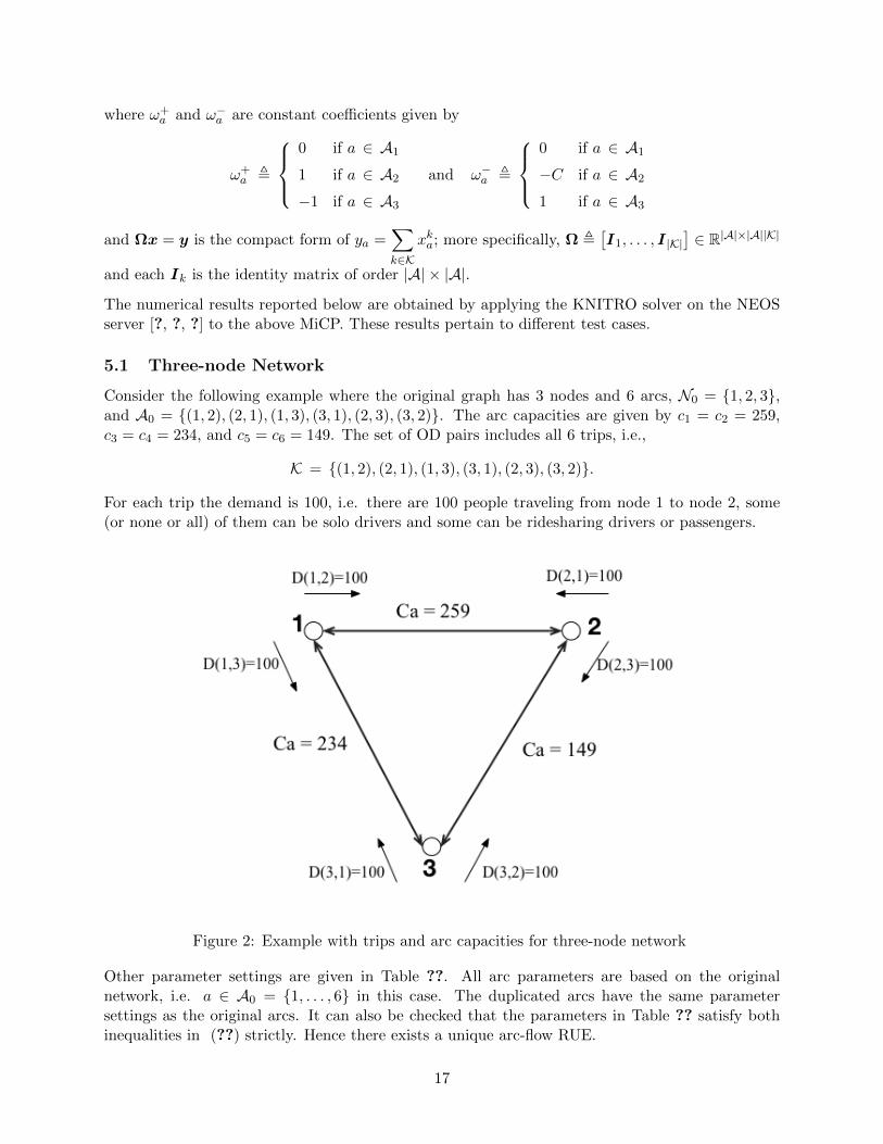
Consider the following example where the original graph has 3 nodes and 6 arcs, N0 = 1, 2, 3,and A0 = (1, 2), (2, 1), (1, 3), (3, 1), (2, 3), (3, 2). The arc capacities are given by c1 = c2 = 259,c3 = c4 = 234, and c5 = c6 = 149. The set of OD pairs includes all 6 trips, i.e.,

K = (1, 2), (2, 1), (1, 3), (3, 1), (2, 3), (3, 2).

For each trip the demand is 100, i.e. there are 100 people traveling from node 1 to node 2, some(or none or all) of them can be solo drivers and some can be ridesharing drivers or passengers.

Figure 2: Example with trips and arc capacities for three-node network

Other parameter settings are given in Table ??. All arc parameters are based on the originalnetwork, i.e. a ∈ A0 = 1, . . . , 6 in this case. The duplicated arcs have the same parametersettings as the original arcs. It can also be checked that the parameters in Table ?? satisfy bothinequalities in (??) strictly. Hence there exists a unique arc-flow RUE.

17

Table 1: Parameter settings for three-node networkDescription Constants Values

free flow time ta(a = 1, . . . , 6) 6, 6, 4, 4, 5, 5arc capacity (threshold) ca(a = 1, . . . , 6) 259, 259, 234, 234, 149, 149congestion coefficients b, b ′, e 0.15, 0.015, 0.3inconvenience coefficients β d, β p 0.1inconvenience coefficients γ d, γ p 0.01price coefficients ρ, v, w 0.5, 0.2, 0.1vehicle capacity α, C 2, 4demand Dk(k = 1, . . . , 6) 100

Note that we set b ′ < b making the congestion cost of passengers less than that of the drivers.We also set e < 1, since the contribution of passengers to the congestion cost is considerably lessthan that of drivers. As for the inconvenience costs, we set β d ≥ γ d, under the assumption thatdrivers contribute more on the inconvenience cost of each driver than passengers. In other words,we assume that the inconvenience cost for drivers of adding one passenger is less than addingone ridesharing driver. Similarly, we set β p ≥ γ p, assuming that drivers contribute more on theinconvenience cost of each passenger. β p (or γ p) could be either the same or different from β d

(or γ d). Finally, we set v > w under the assumption that adding one passenger will contributeless to the ridesharing price than adding one driver. With these settings, the results are shown inTable ??, where only the nonzero xka are listed.

Table 2: Computational results for x for the three-node network(k, a) xka1 (k, a) xka2 (k, a) xka3(1, T1(1)) 81.1756 (1, T2(1)) 9.4122 (1, T3(1)) 9.4122(2, T1(3)) 87.4147 (2, T2(3)) 6.2927 (2, T3(3)) 6.2927(3, T1(2)) 81.1756 (3, T2(2)) 9.4122 (3, T3(2)) 9.4122(4, T1(5)) 83.7752 (4, T2(5)) 8.1124 (4, T3(5)) 8.1124(5, T1(4)) 87.4147 (5, T2(4)) 6.2927 (5, T3(4)) 6.2927(6, T1(6)) 83.7752 (6, T2(6)) 8.1124 (6, T3(6)) 8.1124

The values of the multipliers are η+1 = η+2 = 3.08221, η+3 = η+4 = 2.04928, η+5 = η+6 = 2.48516, andη−a = 0, for all a ∈ A0 = 1, . . . , 6. The values of µ are omitted. Note that for each arc a ∈ A theflow on a comes from only one OD pair, therefore ya equals to the corresponding xka with the samea. The values of ya, fa(y) and Θa,k(x) are given in Table ??, where

Θa,k(x) , fa(Ωx) + ω+a η

+T0(a) + ω−a η

−T0(a) − µ

ki + µkj , ∀a = (i, j) ∈ A,∀k ∈ K

Note that we only care about those Θa,k(x) for which xka is nonzero.

Since every path consists of only one arc, the path cost equals to the corresponding arc cost. Foreach OD pair, the generalized cost of each path, which is calculated by fa(Ωx)+ω+

a η+T0(a)+ω

−a η−T0(a),

equals to the same constant. For example, when k = 1, there are altogether three paths, usingarcs a = 1, 2, 3, respectively. This means that, 81.1756 out of the 100 travelers are driving alonefrom node 1 to node 2, while 9.4122 are taking on passengers and the rest 9.4122 are travelingas passengers. The travel costs experienced by each traveler for the different travel modes aref2(y) + η+1 − Cη

−1 = f3(y)− η+1 + η−1 = f1(y) = 6.0134.

18

Table 3: Computational results for y and the costs for the three-node network

a ya fa(y) Θa,k(x) a ya fa(y) Θa,k(x)

T1(1) 81.1756 6.0134 0.0000 T1(4) 87.4147 4.0153 0.0000T2(1) 9.4122 2.9312 0.0000 T2(4) 6.2927 1.9660 0.0000T3(1) 9.4122 9.0956 0.0000 T3(4) 6.2927 6.0646 0.0000T1(2) 81.1756 6.0134 0.0000 T1(5) 83.7752 5.1080 0.0000T2(2) 9.4122 2.9312 0.0000 T2(5) 8.1124 2.6228 0.0000T3(2) 9.4122 9.0956 0.0000 T3(5) 8.1124 7.5931 0.0000T1(3) 87.4147 4.0153 0.0000 T1(6) 83.7752 5.1080 0.0000T2(3) 6.2927 1.9660 0.0000 T2(6) 8.1124 2.6228 0.0000T3(3) 6.2927 6.0646 0.0000 T3(6) 8.1124 7.5931 0.0000

Under the ridesharing user equilibrium, the generalized costs experienced by each traveler of thesame OD pair are the same, although their travel costs fa(y) may vary. Moreover, it can beseen that all paths are saturated from the perspective of the ridesharing drivers. Therefore eventhough ridesharing drivers are experiencing the least travel costs, others cannot switch to become aridesharing driver. From the perspective of passengers, their travel costs are the highest. But sincetheir path is saturated below, people cannot leave this path for cheaper-cost paths. It can also becalculated from Table ?? that on average, the proportions of solo drivers, ridesharing drivers andpassengers on each arc are, respectively, 84.12% : 7.94% : 7.94%.

5.2 The Braess Network

One interesting test case for the traffic equilibrium problems is the Braess network (see Figure ??).In the original graph, N0 = 1, 2, 3, 4, A0 = (1, 3), (1, 4), (3, 2), (3, 4), (4, 2) (for simplicity,rewrite A0 = 1, . . . , 5), and there is only one OD pair K = (1, 2) with demand D(1, 2) = 6.

Figure 3: Example with trips and free flow travel times for Braess

19

The free flow time is also labeled by each arc in Figure ??, i.e. t1 = t5 = 0.00000001 ≈ 0,t2 = t3 = 50 and t4 = 10. Other parameter settings are given in Table ??. For the Braess network

the exponent in the BPR function is set to 1, fa(y) = ta

[1 + b

(ya1 + ya2

ca

)]for the drivers and

fa(y) = ta

[1 + b ′

(ya1 + ya2 + eya3

ca

)]for the passengers.

Table 4: Parameter settings for the Braess networkDescription Constants Values

free flow time ta(a = 1, . . . , 5) 0, 50, 50, 10, 0arc capacity (threshold) ca(a = 1, . . . , 5) 1congestion coefficients ba(a = 1, . . . , 5) 109, 0.02, 0.02, 0.1, 109

congestion coefficients b ′a, e 0.1ba, 0.3inconvenience coefficients β d, β p 0.1inconvenience coefficients γ d, γ p 0.01price coefficients ρ, v, w 0.5, 0.2, 0.1vehicle capacity α, C 2, 4demand D1 (1→ 2) 6

The Braess network leads to some interesting paradoxes in network flows. Consider the simplestcase: suppose all travelers are solo drivers. Every traveler will observe a travel cost of 10 on path“1→ 3→ 4→ 2” before traveling. Since each of them acts selfishly, all of them will travel on thatpath. As a result, the cost would increase to 60 due to congestion. If they cooperate, they couldreduce the travel cost to 50 for each of them. Now consider our ridesharing case, where travelersmay choose to be a solo driver, a ridesharing driver or a passenger. Given the above parametersettings for the network, the computational results are shown in Table ??. Note that there is onlyone OD pair (1→ 2), hence all ya equal xa.

Table 5: Computational results for the Braess network

a xa = ya fa(y) Θa,k(x)

T1(1) 0.0 12.000 XT2(1) 1.2 11.688 0.000T3(1) 4.8 3.048 0.000T1(2) 0.0 50.000 XT2(2) 0.0 0.000 XT3(2) 0.0 75.000 XT1(3) 0.0 50.000 XT2(3) 0.0 0.000 XT3(3) 0.0 75.000 XT1(4) 0.0 11.200 XT2(4) 1.2 0.888 0.000T3(4) 4.8 15.672 0.000T1(5) 0.0 12.000 XT2(5) 1.2 11.688 0.000T3(5) 4.8 3.048 0.000

20

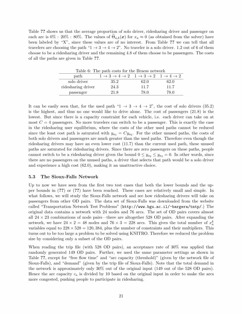
Table ?? shows us that the average proportion of solo driver, ridesharing driver and passenger oneach arc is 0% : 20% : 80%. The values of Θa,k(x) for xa ≈ 0 (as obtained from the solver) havebeen labeled by “X”, since these values are of no interest. From Table ?? we can tell that alltravelers are choosing the path “1→ 3→ 4→ 2”. No traveler is a solo driver. 1.2 out of 6 of themchoose to be a ridesharing driver and the remaining 4.8 of them choose to be passengers. The costsof all the paths are given in Table ??.

Table 6: The path costs for the Braess networkpath 1 → 3 → 4 → 2 1 → 3 → 2 1 → 4 → 2

solo driver 35.2 62.0 62.0ridesharing driver 24.3 11.7 11.7

passenger 21.8 78.0 78.0

It can be easily seen that, for the used path “1 → 3 → 4 → 2”, the cost of solo drivers (35.2)is the highest, and thus no one would like to drive alone. The cost of passengers (21.8) is thelowest. But since there is a capacity constraint for each vehicle, i.e. each driver can take on atmost C = 4 passengers. No more travelers can switch to be a passenger. This is exactly the casein the ridesharing user equilibrium, where the costs of the other used paths cannot be reducedsince the least cost path is saturated with ya3 = Cya2 . For the other unused paths, the costs ofboth solo drivers and passengers are much greater than the used paths. Therefore even though theridesharing drivers may have an even lower cost (11.7) than the current used path, these unusedpaths are saturated for ridesharing drivers. Since there are zero passengers on these paths, peoplecannot switch to be a ridesharing driver given the bound 0 ≤ ya2 ≤ ya3 = 0. In other words, sincethere are no passengers on the unused paths, a driver that selects that path would be a solo driverand experience a high cost (62.0), making it an unattractive choice.

5.3 The Sioux-Falls Network

Up to now we have seen from the first two test cases that both the lower bounds and the up-per bounds in (??) or (??) have been reached. These cases are relatively small and simple. Inwhat follows, we will study the Sioux-Falls network and see how ridesharing drivers will take onpassengers from other OD pairs. The data set of Sioux-Falls was downloaded from the websitecalled “Transportation Network Test Problems” (http://www.bgu.ac.il/~bargera/tntp/.) Theoriginal data contains a network with 24 nodes and 76 arcs. The set of OD pairs covers almostall 24 × 23 combinations of node pairs—there are altogether 528 OD pairs. After expanding thenetwork, we have 24 × 2 = 48 nodes and 76 × 3 = 228 arcs. This gives the total number of xkavariables equal to 228× 528 = 120, 384, plus the number of constraints and their multipliers. Thisturns out to be too large a problem to be solved using KNITRO. Therefore we reduced the problemsize by considering only a subset of the OD pairs.

When reading the trip file (with 528 OD pairs), an acceptance rate of 30% was applied thatrandomly generated 149 OD pairs. Further, we used the same parameter settings as shown inTable ??, except for “free flow time” and “arc capacity (threshold)” (given by the network file ofSioux-Falls), and “demand” (given by the trip file of Sioux-Falls). Note that the total demand inthe network is approximately only 30% out of the original input (149 out of the 528 OD pairs).Hence the arc capacity ca is divided by 10 based on the original input in order to make the arcsmore congested, pushing people to participate in ridesharing.

21

http://www.bgu.ac.il/~bargera/tntp/

The values of ya, η+a and η−a can be found in the Appendix, where we see that the ridesharingcapacity constraint is satisfied for each original arc a0 ∈ A0, i.e. ya2 ≤ ya3 ≤ Cya2 , for all a0 ∈ A0,a2 = T2(a0), and a3 = T3(a0). For most arcs, these constraints hold strictly with the correspondingη+a = η−a = 0. Only for arc a = 46 ∈ A0, we have η+a = 0.3773 > 0 and ya2 = ya3 , meaning thearc is saturated for ridesharing drivers or passengers. On this arc, we can see the costs of solodrivers, ridesharing drivers and passengers, which are 4.3426, 3.9653 and 4.7200, respectively. Inother words, the cost of ridesharing drivers are the lowest among the three. That is why the flowis saturated above for ridesharing drivers on this arc. For all other arcs, the costs of both driversare always the same, and it is either larger or smaller than the cost for passengers.

Figure 4: Proportions of solo drivers, ridesharing drivers and passengers for Sioux-Falls

In particular, Figure ?? shows the proportion of each role (solo driver, ridesharing driver or pas-senger) for each arc in the original graph. According to our model, it is impossible to calculatesuch proportions for each OD pair because people may change roles throughout their travel. Thatis, one traveler may be switching from a solo driver to a ridesharing driver along the (actual)path. Or in our model description, one path may contain arcs from different arc sets A1 and A2.Figure ?? helps us to understand the distribution of the different roles at a point where travelerswill not change roles in a single arc. From this figure, we can see that for some arcs, there arevery few people participating in the ridesharing activities, while for some other arcs, the sum ofthe number of ridesharing drivers and passengers makes up more than half of the total number oftravelers passing those arcs. In general, the arcs with higher proportions of solo drivers usuallyhave lower proportions of ridesharing drivers and passengers. For example, compare arc #1 andarc #21, which could indicate that arc #21 is relatively less crowded than arc #1 so less peopleare participating in ridesharing. However, there are also exceptions – see arc #33 and arc #35.Arc #35 has higher proportion of solo drivers and lower proportion of passengers, yet it has higherproportion of ridesharing drivers than arc #33. So an increase in solo drivers (proportion) doesnot necessarily result in a decrease in both ridesharing drivers and passengers.

22

Also if we take the average of the amount of flow on each type of arc, we can see (from Figure ??)that on average, the proportions of solo drivers, ridesharing drivers and passengers are 70%, 9%,and 21%. In other words, on average 21% of the travelers will become passengers, reducing thetraffic congestion by 21% in the amount of travelers.

Figure 5: Average proportions of solo, ridesharing drivers and passengers for Sioux-Falls

5.3.1 Path selection analysis

In the test cases of the three-node network and the Braess network, it is not clear if ridesharingdrivers have been taking on passengers from other OD pairs. It is because either the network istoo simple (Three-node) or there is only one OD pair (Braess). Therefore with the network ofSioux-Falls, we may analyze such activities among the different OD pairs.

Consider only arcs 1, 2 ∈ A0 in the original graph (see Figure ??), i.e. arc “1 → 2” labeled by “1”and arc “1 → 3” labeled by “2”.Table ?? gives the detailed flow distribution xka over all OD pairs on these two arcs. In this table,the rows are for OD pairs k ∈ K and the columns are for arcs a ∈ A (after extension). OD pairswith zero flow on these arcs are omitted.

From Table ?? we can see that all the passengers on arc “1 → 2” come from OD pair k = 12, i.e.starting from node 3 and traveling to node 8. The number of passengers (96.12) on this arc is farabove the capacity that the ridesharing drivers (4.47) from the same OD pair (k = 12) can take on.On the other hand, there are several other OD pairs, such as k = 2, 7, 66, 67, etc., that do not havepassengers, but have ridesharing drivers traveling from node 1 to node 2. These drivers will takeon the rest of the passengers that those 4.47 drivers from OD pair k = 12 could not. Similarly, onarc “1 → 3”, OD pairs k = 3, 5, 36 contribute a total of 96.06 passengers, which will be spread outto drivers from the other OD pairs.

It is interesting to note that some seemingly unrelated OD pairs are also using arcs “1 → 2” and“1 → 3”. For instance, when k = 88, traveling from node 17 to node 2, some travelers will maketheir path through arc “1 → 2”. Note that from the input file the demand, or the total number oftravelers, of this OD pair is 200, which is much greater than the number of travelers on arc “1 →2”, i.e. 66.71 + 5.31 = 72.02. This indicates that drivers will make a detour like this due to traffic

23

Figure 6: The original network of Sioux-Falls

congestion, or to pick up passengers from other OD pairs for their own benefit.

5.3.2 Sensitivity analysis

As mentioned earlier in Subsection ??, for the instance of the Sioux-Falls network solved, we didnot adopt the original full input but took only a subset of the OD pairs; we also reduced the arccapacities by ten times. These settings can have an impact on the solution, or the distribution ofthe flows, i.e. how people will choose their paths. Hence we are interested in checking how thesolution will change according to different parameter settings.

Changing the arc capacities ca. The capacity of each arc ca is essential to the solution of themodel, since it helps to determine the congestion cost for every traveler, which will interfere with

24

Table 7: Selected xka on the first two original arcs for Sioux-Falls

k ok dkarc “1” ∈ A0, 1 → 2 arc “2” ∈ A0, 1 → 3(1,2)1 (1,2)2 (1,2)3 (1,3)1 (1,3)2 (1,3)3

1 1 5 0.00 0.00 0.00 196.24 3.76 0.002 1 6 294.34 5.66 0.00 0.00 0.00 0.003 1 11 0.00 0.00 0.00 490.16 3.81 6.034 1 13 0.00 0.00 0.00 496.19 3.81 0.005 1 14 0.00 0.00 0.00 273.05 3.78 23.166 1 19 0.00 0.00 0.00 296.21 3.79 0.007 1 20 171.69 5.58 0.00 119.01 3.72 0.009 2 9 0.00 0.00 0.00 196.24 3.76 0.00

10 2 11 0.00 0.00 0.00 196.24 3.76 0.0012 3 8 19.90 4.47 96.12 0.00 0.00 0.0027 6 13 0.00 0.00 0.00 196.24 3.76 0.0033 6 21 0.00 0.00 0.00 96.31 3.69 0.0034 6 22 0.00 0.00 0.00 33.74 3.45 0.0036 7 3 0.00 0.00 0.00 29.74 3.40 66.8666 12 16 657.07 5.72 0.00 0.00 0.00 0.0067 12 18 160.58 5.57 0.00 0.00 0.00 0.0078 15 2 94.56 5.44 0.00 0.00 0.00 0.0088 17 2 66.71 5.31 0.00 0.00 0.00 0.00

132 22 2 94.56 5.44 0.00 0.00 0.00 0.00146 24 6 69.64 5.33 0.00 0.00 0.00 0.00

ya 1629.04 48.53 96.12 2619.35 44.50 96.06

people’s decision on which type of role to travel. In the BPR functions (??) and (??), i.e.

tta (y) = ta

(1 + b

(ya1 + ya2

ca

)4), a ∈ A1 ∪ A2

tt pa (y) = ta

(1 + b ′

(ya1 + ya2 + eya3

ca

)4), a ∈ A3

the arc capacity ca acts as a threshold of the amount of flow on that arc. If the amount of flowis equal to or below ca, the congestion cost on arc a would be close to its free flow time ta. Ifbigger, however, the congestion cost would increase dramatically as the amount of flow increases.Therefore, if ca decreases, i.e. the threshold decreases, the arcs would become more congested underthe same amount of flow. This would push more travelers to participate in ridesharing activities,meaning an increase in the number of both ridesharing drivers and passengers and thus a decreasein the number of solo drivers.

Table ?? shows the changes with ca for the different networks. In the table, D denotes the average

demand, i.e. D ,1

|K|∑k∈K

Dk. This average can help understand how many people are traveling on

the road. Thus we set ca to be proportional to 0.1D, D and 10D, respectively. The triplet in eachcell gives the proportions (in %) of solo drivers (SD), ridesharing drivers (RD), and passengers (P).As expected, when ca increases (from ∼ 0.1D to ∼ 10D), the proportion of solo drivers increases

25

while that of ridesharing drivers and passengers decreases. Note that other parameters remainunchanged in this subsection. It can be summarized from Table ?? that when the traffic becomesless congested (as ca increases), fewer people would participate in ridesharing.

Table 8: Ridesharing proportions (%) with arc capacity changes

ca ∼ 0.1D ca ∼ D ca ∼ 10DTest case % SD % RD % P % SD % RD % P % SD % RD % P

Three-node 9.60 31.80 58.61 84.12 7.94 7.94 84.37 7.81 7.81Braess 0.00 20.00 80.00 0.00 20.00 80.00 20.67 29.33 50.00Sioux-Falls 15.56 22.82 61.62 70.27 8.38 21.35 99.56 0.22 0.22

When ca increases, i.e. the congestion cost decreases, more people would become solo driverswhile less people will become ridesharing passengers. Note that as the arc capacity increases, theproportion of ridesharing drivers may increase or decrease, but overall the adoption of ridesharing,i.e. the sum of the proportion of ridesharing drivers and passengers, still decreases.

Changing the inconvenience parameters β d, γ d, β p, γ p. The convenience costs of ridesharingfor both drivers and passengers are defined in Section ?? by (??) and (??), respectively, i.e.

I da (y) = β d ya2 + γ d ya3 , a ∈ A2

I pa (y) = β p ya2 + γ p ya3 , a ∈ A3.

They are both (linearly) increasing functions of the amount of flow (note that all coefficients arepositive). Intuitively, when the inconvenience cost increases, the cost of ridesharing goes up forboth drivers and passengers. Hence less people would like to participate in ridesharing; and viceversa.

Note that all the parameters of the inconvenience costs β d, γ d, β p, γ p must satisfy the constraintsin (??) to ensure the uniqueness of the arc-flow solution. Thus define

Con1 , 4(β d + αv)(γ p + w)− (γ d − αw + β p − v)2

Con2 , 4eb− b′(1 + eC)3.

When changing any parameters involved above, we need to check if the two inequalities (??) areviolated. In changing the arc capacities ca, however, there is no need to check these constraintssince ca is not involved. In the previous tests, (β d, γ d, β p, γ p) is set to be (0.1, 0.01, 0.1, 0.01).To compare with this settings while maintaining the above two constraints, we multiply (β d, γ d,β p, γ p) by 0.1 and 10, respectively.

The three sets of parameter values are listed in Table ?? and the test results are given in Table ??.We can see that all three sets of (β d, γ d, β p, γ p) satisfy the two parameter requirements (due topositive Con1 and Con2 values). The column title (0.01, 0.001) represents the set (β d = β p = 0.01,γ d = γ p = 0.001).In the result of Table ??, ca is set to ∼ 0.1D in the “Three-node” network, ∼ 10D in the “Braess”network, and D in the “Sioux-falls” network. This is because the original setting ca ∼ D forthe first two networks will give ridesharing flows that touch their upper/lower bounds (saturatedarcs/paths). These are extreme cases for ridesharing activities where the actual travel costs (NOTthe generalized cost) of different travelers are not equal at the equilibrium. Hence different ca values

26

Table 9: Parameter settings and constraint checks for inconvenience parameter changesβd γd βp γp α C ρ v w e Con1 Con2

0.01 0.001 0.01 0.001 2 4 0.5 0.2 0.1 0.3 0.0143 0.13520.1 0.01 0.1 0.01 2 4 0.5 0.2 0.1 0.3 0.1359 0.13521 0.1 1 0.1 2 4 0.5 0.2 0.1 0.3 0.6300 0.1352

Table 10: Ridesharing proportions (%) with inconvenience parameter changes(β, γ) ( 0.01, 0.001 ) (0.1, 0.01) (1, 0.1)Test case % SD % RD % P % SD % RD % P % SD % RD % P


are selected for the “Three-node” network and the “Braess” network to eliminate this influence. Weonly consider the situation where the vehicle capacity constraints hold strictly, and thus drivers andpassengers may switch roles more willingly. Despite different ca values for the different networks, allthe parameter settings remain fixed except for the inconvenience-cost parameters (βd, γd, βp, γp).

From Table ?? we can see that as the inconvenience cost increases, i.e. parameter settings changesfrom (0.01, 0.001) to (1, 0.1), the proportion of ridesharing decreases (including both drivers andpassengers), which meets our expectation. When the inconvenience cost increases, more peoplewould become solo drivers while less people will become ridesharing drivers or passengers.

Changing the pricing parameters ρ, v, w. Changing the pricing parameters can be trickycompared to changing the other parameters. When the price increases, it is appealing for moretravelers to become ridesharing drivers. At the same time, however, it may lose passengers aswell due to a higher cost being a passenger. Therefore the proportion of ridesharing can either beincreasing or decreasing with the changes of pricing parameters.

Same as before, we kept the other parameters fixed while changing any pricing parameters. We setca ∼ 0.1D for the “Three-node” network, ca ∼ 10D for “Braess” and ca ∼ D for “Sioux-Falls”. Still,we set b ′ = 0.1b for all arcs in all networks. The sets of parameter values are listed in Table ?? andwe can see that all parameter settings satisfy all the parameter constraints. The obtained resultsare given in Table ??.

Table 11: Parameter settings and constraint checks for pricing parameter changesβd γd βp γp α C ρ v w e Con1 Con2

0.1 0.01 0.1 0.01 2 4 0.05 0.02 0.01 0.3 0.0063 0.13520.1 0.01 0.1 0.01 2 4 0.5 0.2 0.1 0.3 0.1359 0.13520.1 0.01 0.1 0.01 2 4 5 2 1 0.3 1.4319 0.1352

From Table ??, we can see that, when the pricing parameters increase there is a significant increasein the number or proportion of ridesharing drivers, while that of passengers decreases as expected.The proportion changes of solo drivers to the pricing parameters are not obvious.

• For “Three-node”, the proportion of solo drivers keeps decreasing with the increase of pricingparameters. This means that the benefit as a ridesharing driver appears to be so compelling

27

Table 12: Ridesharing proportions (%) with pricing parameter changes(ρ, v, w) (0.05, 0.02, 0.01) (0.5, 0.2, 0.1) (5, 2, 1)Test case % SD % RD % P % SD % RD % P % SD % RD % P


that both solo drivers and passengers would switch to be a ridesharing driver.

• For “Braess”, the proportion of solo drivers increases when the price parameters increasefrom (0.05, 0.02, 0.01) to (0.5, 0.2, 0.1), because this change has more of an impact onpassengers than on drivers, and thus more passengers are switching to solo drivers than toridesharing drivers. In other words, the decrease of the proportion of passengers overcomesthe increase of the proportion of ridesharing drivers. Therefore the overall proportion ofridesharing decreases, which leads to an increase of solo drivers.

• For “Sioux-Falls”, the proportion of solo drivers keeps increasing with the increase of theridesharing price parameters. Similar to the first half of the case for “Braess”, an increase inthese parameters pushes more passengers to drive alone than to drive with other passengers.

Summary. The changes with the parameter settings can be summarized in Table ??, wherethe first column represents different traveler roles (“ridesharing (total)” includes both ridesharingdrivers and ridesharing passengers), and the second to the fourth columns give the proportionchanges for each role under different parameter changes.

Table 13: The impact of parameter changes on ridesharing proportionsProportion changes arc capacity ↑ inconvenience cost ↑ pricing parameters ↑

solo driver ↑ ↑ undetermined

ridesharing (total) ↓ ↓ undetermineddriver undetermined ↓ ↑

passenger ↓ ↓ ↓

It can be observed from Table ?? that

1. When the arc capacity increases, more people would become solo drivers and thus less peoplewould participate in ridesharing. Passengers will become solo drivers or ridesharing drivers.

2. When the inconvenience cost increases, more people would become solo drivers and thus lesspeople would participate in ridesharing. In particular, both the number of ridesharing driversand passengers will decrease due to an increased cost.

3. When the ridesharing price parameters increase, more people would become ridesharingdrivers and less people would become ridesharing passengers. The number of solo driversis undetermined, that is, it is possible that more passengers are switching to solo drivers, andit is also likely that more solo drivers would become ridesharing drivers.

These sensitivity results validate that the proposed model correctly captures reasonable behavior,such as increasing arc capacity leads to an increase in solo drivers and decrease in ridesharing

28

passengers. However, there are some unexpected or undetermined results. For example increasingridesharing pricing parameters for the Sioux-Falls network example does not have a marked effecton the number of solo drivers and total ridesharing. This implies that if a planner forces an increasein ridesharing price, attempting to make ridesharing drivers more attractive, it could lead to anoverall increase in drivers and a reduction in total ridesharing, increasing congestion.

6 Conclusions

This paper proposes VI/CP models for solving the traffic equilibrium problem with ridesharing.The mathematical models developed explicitly take into account how the notion of shortest pathhas to be adapted to include the costs/benefits of ridesharing and provide a method to quantifythese costs. These models determine how travelers will behave given a transportation system withridesharing services, and hence help city planners to design certain conditions according to travelers’behavior in order to reduce traffic congestion. In our study, we made some assumptions, such as(a) the drivers and passengers that are sharing the same car may travel on different OD pairs;(b) there is a vehicle capacity constraint for all ridesharing vehicles. In order to cope with (a),the travel network is extended by doubling the size of the node set and tripling the size of thearc set; to handle (b), a generalized traffic equilibrium is defined and is formulated as a mixedcomplementarity problem and also equivalently as a variational inequality. The latter is shownto have a unique solution. The KNITRO solver is adopted to solve the resulting MiCP. Thecomputational results are also promising, as not only do they validate some intuitive guesses, butalso provide new insights to some unexpected conclusions.

Future challenges may include: (1) an individual level transportation equilibrium model withridesharing, such that the assignment of each passenger may be captured; (2) an inconveniencecost based on paths instead of arcs; (3) more transit modes (like public transit) for travelers tochoose from; (4) elastic traffic demand where travelers may choose not to travel if no transit modesmeet their needs; etc.

Acknowledgment

The work of Xu, Dessouky, and Ordonez was based on research supported by the Federal HighwayAdministration under the Broad Agency Announcement of Exploratory Advanced Research (EAR).The work of Pang was based on research supported by the U.S. National Science Foundation undergrant CMMI-1402052.

References

[1] Aashtiani, H. and Magnanti, T. Equilibria on a congested transportation network. SIAMJournal on Algebraic Discrete Methods 2 (1981) 213–226.

[2] Agdeppa, R.P., Yamashita, N., and Fukushima, M. The traffic equilibrium problemwith nonadditive costs and its monotone mixed complementarity problem formulation. Trans-portation Research Part B: Methodological 41 (2007) 862–874.

[3] Amey, A. Real-time ridesharing : exploring the opportunities and challenges of designinga technology-based rideshare trial for the MIT community. Master’s thesis. MassachusettsInstitute of Technology (2010).

29

[4] Ban, X., Liu, H., Ferris, M.C., and Ran, B. A link-node complementarity model andsolution algorithm for dynamic user equilibria with exact flow propagations. TransportationResearch, Part B: Methodological 9 (2008) 823–842.

[5] BTS Transportation Statistics Annual Report 2012. U.S. Department of Transportation, Re-search and Innovative Technology Administration Bureau of Transportation Statistics. (2013).

[6] Burris, M. and Winn, J. Slugging in Houston-Casual carpool passenger characteristics.Journal of Public Transportation 9 (2006) 23–40.

[7] Byrd, R., Hribar, M.E., and Nocedal, J. An interior point method for large scalenonlinear programming. SIAM Journal on Optimization 4 (1999) 877–900.

[8] Byrd, R.H., Nocedal, J., and Waltz, R.A. KNITRO: An Integrated Package for Non-linear Optimization In G. Di Pillo and R. Noma, editors. Large-Scale Nonlinear Optimization83 (2006) pp. 35–59.

[9] Chan, N. and Shaheen, S. Ridesharing in North America: past, present, and future.Transport Reviews 32 (2012) 93–112.

[10] Czyzyk, J., Mesnier, M., and More, J. The NEOS server. IEEE Journal on Computa-tional Science and Engineering 5 (1998) 68–75.

[11] Dafermos, S.C. Traffic equilibrium and variational inequalities. Transportation Science 14(1980) 4254.

[12] Dailey, D.J., Loseff, D., and Meyers, D. Seattle smart traveler: dynamic ridematchingon the World Wide Web. Transportation Research Part C: Emerging Technologies 7 (1999)17–32.

[13] Dolan, E. The NEOS server 4.0 administrative guide. Mathematics and Computer ScienceDivision, Argonne National Laboratory, Technical Memorandum ANL/MCS-TM-250 (2001).

[14] Facchinei, F. and Pang, J.S. Finite-Dimensional Variational Inequalities and Comple-mentarity Problems. Springer (New York 2003).

[15] Ferguson, E. The rise and fall of the American carpool: 1970–1990. Transportation 24(1997) 349–376.

[16] Ferris, M.C. and Munson, T.S. Interfaces to PATH 3.0: Design, Implementation andUsage. Computational Optimization and Applications 12 (1999) 207–227.

[17] Furuhata, M., Dessouky, M.M., Ordonez, F., Brunet, M., Wang, X., and Koenig,S. Ridesharing: the state-of-the-art and future directions. Transportation Research Part B:Methodological 57 (2013) 28–46.

[18] Ghoseiri, K., Haghani, A., and Hamedi, M.. Real-time rideshare matching problem.Department of Civil and Environmental Engineering, University of Maryland College Park(January 2011).

[19] Gropp, W. and More, J. Optimization environments and the NEOS server. In Buhmann,M.D. and Iserles, A., editors. Approximation Theory and Optimization, Cambridge UniversityPress (1997) pp. 167–182.

30

[20] Heinrich, S. Implementing real-time ridesharing in the San Francisco bay area. Master’sthesis, Mineta Transportation Institute, San Jose State University (2010).

[21] Hubbard, R.G. and O’Brien, A.P. Economics. Fourth edition. Prentice Hall (2012).

[22] Kelley, K. Casual carpooling—enhanced. Journal of Public Transportation 10 (2007) 119–130.

[23] Jayakrishnan, R., Tsai, W.K., Prashker, J.N., and Rajadhyaksha, S. A faster path-based algorithm for traffic assignment. Transportation Research Record 1443 (1994) 75–83.

[24] Larsson, T. and Patriksson, M. Side constrained traffic equilibrium models–analysis,computation and applications. Transportation Research Part B: Methodological 33 (1999)233–264.

[25] Larsson, T. and Patriksson, M. Equilibrium characterizations of solutions to side con-strained asymmetric traffic assignment models. Le Matematiche 49 (1994) 249–280.

[26] LeBlanc, D. Slugging: The Commuting Alternative for Washington DC. Forel Publishing(1999).

[27] Levofsky, A. and Greenberg, A. Organized dynamic ride sharing: The potential envi-ronmental benefits and the opportunity for advancing the concept. Transportation ResearchBoard Annual Meeting (2001).

[28] Lu, S.. Sensitivity of static traffic user equilibria with perturbations in arc cost function andtravel demand. Transportation Science 42 (2008) 105–123.

[29] Morency, C. The ambivalence of ridesharing. Transportation 34 (2007) 239–253.

[30] Nie, Y. A note on Bar-Gera’s algorithm for the origin-based traffic assignment problem.Transportation Science 46 (2012) 27–38.

[31] Patriksson, M. The Traffic Assignment Problem: Models and Methods. CRC Press (1994).

[32] Qian, Z. and Zhang, H.. Modeling multi-modal morning commute in a one-to-one corridornetwork. Transportation Research Part C: Emerging Technologies 19 (2011) 254–269.

[33] Schrank, D., Eisele, W., and Lomax, T. 2012 Urban Mobility Report. TexasA&M Transportation Institute. http://d2dtl5nnlpfr0r.cloudfront.net/tti.tamu.edu/documents/mobility-report-2012.pdf.

[34] Spielberg, F. and Shapiro, P. Mating habits of slugs: Dynamic carpool formation in theI-95/I-395 corridor of Northern Virginia. Transportation Research Board 1711 (2000) 31–38.

[35] Wardrop, J. Some theoretical aspects of road traffic research. Proceeding of the Instituteof Civil Engineers, Part II 1 (1952) 325–362.

[36] Xu, H. Traffic Assignment Models for a Ridesharing Transportation Market. Ph.D. Thesis.Department of Industrial and Systems Engineering, University of Southern California (June2014).

[37] Xu, H., Ordonez, F., and Dessouky, M. A traffic assignment model for a rideshar-ing transportation market. Journal of Advanced Transportation (December 2014) doi:10.1002/atr.1300.

31

http://d2dtl5nnlpfr0r.cloudfront.net/tti.tamu.edu/documents/mobility-report-2012.pdf

http://d2dtl5nnlpfr0r.cloudfront.net/tti.tamu.edu/documents/mobility-report-2012.pdf

[38] Yang, H. and Huang, H.. Carpooling and congestion pricing in a multilane highway withhigh-occupancy-vehicle lanes. Transportation Research Part A: Policy and Practice 33 (1999)139–155.

APPENDIX: KNITRO Outputs – Sioux Falls, 149 OD pairs

a ya1 ya2 ya3 η+a η−a fa1 fa2 fa31 1,629.04 48.53 96.12 0.0000 0.0000 6.1584 6.1584 14.73752 2,619.35 44.50 96.06 0.0000 0.0000 5.0071 5.0071 12.22163 1,532.91 37.41 66.86 0.0000 0.0000 6.1216 6.1216 12.62704 1,207.02 198.53 496.12 0.0000 0.0000 53.4338 53.4338 49.46495 2,055.77 44.53 96.12 0.0000 0.0000 4.3892 4.3892 12.16166 4,403.41 172.21 432.12 0.0000 0.0000 34.6830 34.6830 39.74407 4,694.50 67.60 156.85 0.0000 0.0000 14.2855 14.2855 17.56318 4,702.76 169.48 424.94 0.0000 0.0000 43.4471 43.4471 40.16949 3,882.73 74.19 184.70 0.0000 0.0000 9.3544 9.3544 16.6759

10 1,185.85 183.23 450.61 0.0000 0.0000 60.4557 60.4557 48.180211 3,726.67 53.20 129.47 0.0000 0.0000 8.1239 8.1239 12.559612 1,037.39 86.03 205.35 0.0000 0.0000 19.9440 19.9440 21.959113 3,068.18 460.13 1,184.55 0.0000 0.0000 121.2320 121.2320 108.849014 1,208.29 243.20 613.68 0.0000 0.0000 60.0843 60.0843 59.566115 1,174.97 205.44 519.59 0.0000 0.0000 40.3467 40.3467 48.186516 1,748.55 676.07 1,768.62 0.0000 0.0000 182.0600 182.0600 169.677017 2,328.10 181.63 462.19 0.0000 0.0000 50.2125 50.2125 43.031818 3,376.82 123.78 315.21 0.0000 0.0000 3.5017 3.5017 25.462419 1,678.71 374.44 974.84 0.0000 0.0000 94.5799 94.5799 88.559020 2,398.82 201.78 515.21 0.0000 0.0000 57.4307 57.4307 47.852521 951.38 165.56 383.06 0.0000 0.0000 45.8905 45.8905 45.890522 1,197.77 354.05 905.39 0.0000 0.0000 72.0958 72.0958 84.478423 2,991.64 480.24 1,237.46 0.0000 0.0000 113.9730 113.9730 111.957024 1,016.22 307.36 756.20 0.0000 0.0000 80.7716 80.7716 80.771625 4,046.12 208.74 533.52 0.0000 0.0000 42.3296 42.3296 46.872526 3,123.36 70.79 170.49 0.0000 0.0000 15.4911 15.4911 17.506227 2,970.51 477.57 1,230.45 0.0000 0.0000 111.0170 111.0170 111.017028 4,293.75 822.40 2,132.62 0.0000 0.0000 190.9850 190.9850 190.985029 1,322.91 652.21 1,695.29 0.0000 0.0000 168.3590 168.3590 168.359030 1,067.71 288.76 717.78 0.0000 0.0000 73.3421 73.3421 73.860331 959.45 113.87 268.09 0.0000 0.0000 26.5710 26.5710 29.848632 3,051.02 580.80 1,502.12 0.0000 0.0000 135.4850 135.4850 135.485033 1,161.31 337.90 857.63 0.0000 0.0000 84.3035 84.3035 84.303534 1,329.49 669.18 1,739.96 0.0000 0.0000 173.3090 173.3090 173.309035 3,899.37 24.15 42.49 0.0000 0.0000 8.7395 8.7395 8.739536 1,178.32 304.09 768.66 0.0000 0.0000 80.8532 80.8532 76.490537 4,152.62 139.08 350.21 0.0000 0.0000 6.3925 6.3925 29.488838 3,581.49 32.36 69.36 0.0000 0.0000 4.7056 4.7056 9.068439 1,523.65 521.08 1,350.21 0.0000 0.0000 160.0960 160.0960 134.579040 1,315.36 365.46 940.69 0.0000 0.0000 88.6847 88.6847 88.6847

32

41 1,325.64 549.02 1,418.48 0.0000 0.0000 139.0040 139.0040 139.004042 1,084.33 91.88 220.73 0.0000 0.0000 23.5227 23.5227 23.522743 3,636.57 302.57 764.67 0.0000 0.0000 71.0087 71.0087 71.008744 1,309.14 380.07 973.87 0.0000 0.0000 93.3406 93.3406 93.340645 1,853.05 12.52 17.15 0.0000 0.0000 4.2113 4.2113 5.257346 1,253.13 8.46 8.46 0.3773 0.0000 4.3426 3.9653 4.720047 1,138.61 204.81 512.65 0.0000 0.0000 42.6854 42.6854 49.224648 1,470.19 220.22 558.46 0.0000 0.0000 92.1841 92.1841 58.278649 716.10 38.37 90.46 0.0000 0.0000 3.2993 3.2993 9.262550 4,268.66 53.52 125.06 0.0000 0.0000 13.4697 13.4697 13.987951 1,089.16 389.51 982.92 0.0000 0.0000 100.2660 100.2660 100.266052 1,789.72 404.87 1,054.93 0.0000 0.0000 95.0164 95.0164 94.498253 1,695.39 444.10 1,158.15 0.0000 0.0000 118.0780 118.0780 107.179054 3,498.37 78.22 195.33 0.0000 0.0000 3.6364 3.6364 16.838055 3,843.30 218.22 558.46 0.0000 0.0000 11.1635 11.1635 45.068956 6,326.35 169.27 424.40 0.0000 0.0000 39.6051 39.6051 39.605157 4,006.15 205.61 525.29 0.0000 0.0000 34.4664 34.4664 45.365458 861.91 10.52 17.15 0.0000 0.0000 5.2094 5.2094 4.163459 1,107.55 176.13 442.45 0.0000 0.0000 30.0137 30.0137 40.912760 6,754.61 224.51 569.75 0.0000 0.0000 51.4493 51.4493 51.449361 1,385.32 360.21 926.88 0.0000 0.0000 92.9352 92.9352 87.999462 942.14 99.91 231.34 0.0000 0.0000 22.1889 22.1889 26.551563 1,229.47 230.56 580.42 0.0000 0.0000 56.3484 56.3484 56.348464 1,224.65 503.24 1,292.73 0.0000 0.0000 128.3870 128.3870 128.387065 1,684.28 256.88 665.48 0.0000 0.0000 58.9370 58.9370 58.937066 1,494.27 585.01 1,523.72 0.0000 0.0000 150.6660 150.6660 146.304067 3,436.99 666.24 1,737.48 0.0000 0.0000 153.2380 153.2380 153.238068 1,260.67 284.72 722.94 0.0000 0.0000 69.4498 69.4498 69.449869 1,221.47 76.84 191.68 0.0000 0.0000 13.3935 13.3935 17.756270 1,375.53 458.09 1,184.45 0.0000 0.0000 112.5210 112.5210 112.521071 1,321.24 333.10 855.53 0.0000 0.0000 80.4017 80.4017 80.401772 1,319.43 275.79 704.72 0.0000 0.0000 66.1673 66.1673 66.167373 1,595.90 224.61 580.55 0.0000 0.0000 51.5392 51.5392 51.539274 1,402.69 428.08 1,105.46 0.0000 0.0000 104.3190 104.3190 104.319075 1,125.57 208.48 532.83 0.0000 0.0000 28.0216 28.0216 46.198676 1,247.19 181.52 467.17 0.0000 0.0000 20.7913 20.7913 38.9683

33

Complementarity Models for Traffic Equilibrium with Ridesharing

Documents

Transcript of Complementarity Models for Traffic Equilibrium with Ridesharing