Towards the User Equilibrium in Traffic Assignment UsingGRASP with Path Relinking

Gabriel de O. RamosInstituto de Informática

Universidade Federal do Rio Grande do SulPorto Alegre, RS, Brazil

goramos@inf.ufrgs.br

Ana L. C. BazzanInstituto de Informática

Universidade Federal do Rio Grande do SulPorto Alegre, RS, Brazilbazzan@inf.ufrgs.br

ABSTRACTSolving the traffic assignment problem (TAP) is an impor-tant step towards an efficient usage of the traffic infrastruc-ture. A fundamental assignment model is the so-called UserEquilibrium (UE), which may turn into a complex optimi-sation problem. In this paper, we present the use of theGRASP metaheuristic to approximate the UE of the TAP.A path relinking mechanism is also employed to promote ahigher coverage of the search space. Moreover, we propose anovel performance evaluation function, which measures thenumber of vehicles that have an incentive to deviate from theroutes to which they were assigned. Through experiments,we show that our approach outperforms classical algorithms,providing solutions that are, on average, significantly closerto the UE. Furthermore, when compared to classical meth-ods, the fairness achieved by our assignments is considerablybetter. These results indicate that our approach is efficientand robust, producing reasonably stable assignments.

CCS Concepts•Theory of computation → Optimization with ran-domized search heuristics; Exact and approximate com-putation of equilibria; •Computing methodologies→Ar-tificial intelligence; Search methodologies; Modeling and sim-ulation;

Keywordstraffic assignment, user equilibrium, metaheuristics, GRASP

1. INTRODUCTIONEfficient urban mobility has shown to be a major chal-

lenge towards smart cities. Traditional approaches for deal-ing with arising traffic issues include increasing the physicalcapacity of existing traffic infrastructure. Such approaches,however, have proven unsustainable from many perspectives.Moreover, as stated by the Braess’ paradox [4], expandingthe infrastructure’s capacity may lead to a deterioration in

Permission to make digital or hard copies of all or part of this work for personal orclassroom use is granted without fee provided that copies are not made or distributedfor profit or commercial advantage and that copies bear this notice and the full cita-tion on the first page. Copyrights for components of this work owned by others thanACM must be honored. Abstracting with credit is permitted. To copy otherwise, or re-publish, to post on servers or to redistribute to lists, requires prior specific permissionand/or a fee. Request permissions from permissions@acm.org.

GECCO ’15, July 11 - 15, 2015, Madrid, Spainc© 2015 ACM. ISBN 978-1-4503-3472-3/15/07. . . $15.00

DOI: http://dx.doi.org/10.1145/2739480.2754755

the traffic performance. Against this background, ways ofmaking a more efficient use of the existing infrastructurehave been increasingly studied. Among such ways, trafficassignment is a particularly relevant one.

Traffic assignment represents an important step towardsmodelling and simulating transportation systems. Specifi-cally, the traffic assignment problem (TAP) addresses how toefficiently connect the physical infrastructure (supply) andthe vehicles1 that are going to use it. In other words, bysolving the TAP one can promote a more efficient use of thecurrently available traffic infrastructure.

Solving the TAP, however, is not a trivial task. As a firstattempt, one may consider assigning vehicles to their corre-sponding shortest routes. However, such an approach maylead to the concentration of vehicles in a small number ofroads (a.k.a. links), which might incur in huge congestions.The problem is also unlikely to be overcome by simply cre-ating alternative routes. Due to the limited availability ofresources (links), different routes may share the same links.In other words, the problem is more related to how to effi-ciently spread the traffic than with the number of routes tobe used itself. Precisely, solving the TAP means distribut-ing the vehicles into the road network regarding their originsand destinations (a.k.a. OD pairs) in order to minimise someassociated cost (e.g., travel time, money expenses, pollutingemissions). Therefore, the TAP is essentially an optimiza-tion problem.

Two fundamental traffic assignment models have been de-veloped to solve the TAP: system optimal (SO) and userequilibrium (UE). In an SO approach, one seeks to find anassignment that minimises the travel costs on a global level,i.e., it describes the system at its best operation. However,minimising the global cost may lead to increasing the costof some users. Consequently, some users may have an incen-tive to deviate from the routes to which they were assigned.Hence, an SO solution may be infeasible in practice. TheUE approach, on the other hand, describes solutions fromthe users’ behaviour point of view. In essence, in a UE con-figuration, every user is assigned to one of the best availableroutes for its OD pair. Along these lines, the advantage of aUE solution (over an SO one) is that users have no incentiveto deviate from the routes they were assigned to. Thus, theUE configuration is more likely to be pursued in practice bythe drivers than an SO one.

Many methods have been proposed for solving the TAPusing one or both models described before, each with itsstrengths and weaknesses. What must be clear, however,

1Henceforth, we use the terms vehicle and driver alternately.

is that in both approaches the search space can be hugeand solving the problem optimally may be infeasible. Tothis respect, an alternative that has drawn attention is thedevelopment of methods capable of finding approximate so-lutions to the TAP. Specifically, the use of heuristics in theTAP has shown a promising direction.

In this paper, we approach the TAP in terms of UE withthe GRASP+PR algorithm. GRASP+PR stands for theGreedy Randomised Adaptive Search Procedure algorithmembodied with the Path Relinking mechanism. GRASP isa heuristic search algorithm that greedily builds indepen-dent solutions and improve them with local search. The PRmechanism is used to increase the diversity of solutions. Wepropose a novel representation of solutions, which allows themodelling of TAP in terms of the UE. Through such a rep-resentation, GRASP+PR can be used to minimise the num-ber of vehicles that are assigned to non-least cost routes,thus enhancing the assignments’ fairness. To the best of ourknowledge, this is the first approach to address the UE byminimising the amount of vehicles on non-least cost routes.Our proposal is empirically evaluated, and shown to providesolutions that are, on average, considerably fairer and closerto the UE than those from classical methods. Such resultsshow that our approach is efficient, providing reasonablystable assignments.

The present work is organised as follows. Basic conceptsare introduced in Section 2. A brief overview of related workand the GRASP+PR algorithm are presented in Sections 3and 4, respectively. The problem modelling and the use ofGRASP+PR in our approach are detailed in Section 5. Theevaluation of our proposal is shown in Section 6. Concludingremarks and future directions are presented Section 7.

2. TRAFFIC ASSIGNMENTIn this section, the basic concepts surrounding traffic as-

signment are presented. For a more comprehensive overviewthe reader is referred to [16, chapter 10] or [3, chapter 4].

A road network can be represented as a directed graphG = (N,L), where the set N of nodes represents the inter-sections, and the set L of directed links represents the roadsbetween intersections. Each link lk ∈ L has an associatedcost ck, which is given as a function of some of its attributes,like length, speed limit, capacity, load/flow (of vehicles), etc.The cost of a link represents some sort of measure, like traveltime, money expenses, polluting emissions, etc.

The flow of vehicles in a network (the demand) is basedon the amount of trips made between different origins anddestinations. Let Tij be the demand for trips between origini and destination j, i.e., the number of vehicles that need toreach j from i. The set of all such demands is represented byan origin-destination (OD) matrix T = {Tij | ∀i, j ∈ N, i 6=j, Tij ≥ 0}. A trip is made by means of a route R ⊆ L,which is a sequence of links that connects an origin to adestination. The cost CR of a given route R can be obtainedby summing up the costs of the links that comprise it, as inEquation (1).

CR =∑lk∈R

ck (1)

In order to compute the cost of the links, the concept ofvolume-delay functions (VDF) needs to be introduced. AVDF is a well-known abstraction used to express the delay(cost) of a link depending on the volume (flow) of vehicles on

it. In other words, VDFs provide a means to study how theflow affects the cost on a link. Such a concept is importantbecause the TAP is typically studied in a macroscopic level,i.e., the vehicles movement is considered in an abstract way.A VDF takes as input the flow of vehicles within a link and,based on the characteristics of such link (e.g., length, capac-ity, etc.), returns a cost on it. A simple VDF is presented inEquation (2), with tk and fk representing, respectively, thefree flow travel time (minimum travel time when the link isnot congested), and the number of vehicles on link lk ∈ L.This particular VDF represents the travel time on link k,which is increased by 0.02 for each vehicle/hour of flow.

ck(fk) = tk + 0.02× fk (2)

As previously stated, two fundamental models to solvethe TAP are System Optimal (SO) and User Equilibrium(UE). Recall that an SO assignment describes the systemas its best operation. On the other hand, UE stands forthe traffic condition stated by the Wardrop’s first principle:“under equilibrium conditions traffic arranges itself in con-gested networks such that all used routes between an ODpair have equal and minimum costs while all unused routeshave greater or equal costs” [22]. We refer the reader to [11]for the mathematical formulation of these models. Thatsaid, although the SO model may seem the most efficientone, it has the disadvantage that some users may have noincentive to actually follow the routes to which they wereassigned. In fact, some users would change their routes tothose with minimum cost. Thus, the UE model has showna more realistic way of assigning routes to vehicles.

The UE model can be analytically stated as an optimiza-tion problem. However, this model has the drawback of notbeing solvable algebraically, except for very simple scenar-ios. Hence, providing approximate solutions to the problemhas shown a promising direction. Before advancing to thistopic, some traditional methods need to be introduced.

In general, methods for the TAP involve two steps [16]:(i) using a set of rules to identify desirable routes (e.g., thefastest) in each OD pair (this is usually performed by short-est path algorithms), and (ii) assigning suitable portions ofthe OD trips to these routes so that a given objective isachieved. It should be noted, however, that the desirabilityof a given route may vary due to congestion effects. Specifi-cally, desirable routes may become less attractive than oth-ers as the flow on their links increase. On this basis, thetwo steps above are generally performed iteratively, until agiven (non-iterative) convergence criterion is achieved.

The simplest traffic assignment method is known as all-or-nothing, which perform the task without accounting forcongestion effects. Specifically, the all-or-nothing methodselects the shortest route for each OD pair, and then assignsthe entire corresponding flow to that route. This approach,however, is quite naıve, since assigning all vehicles to thesame routes (one per OD pair) can lead to congestions. Al-though this method is of low interest in practice, it has beenused by more sophisticated methods. Furthermore, it maybe useful as an upper bound.

More sophisticated methods for traffic assignment are it-erative ones, which account for congestion. One of thesemethods is the so-called incremental assignment. The in-cremental assignment method iteratively loads proportionalfractions pn (with

∑n pn = 1) of the demand into the lowest

cost routes (one for each OD pair). A new set of lowest cost

Algorithm 1: Pseudocode of MSA (adapted from [16])

1 select an initial set of current link costs (usually free-flowtravel times); initialise the flow of every link k: fk = 0; setn = 0;

2 create an auxiliary all-or-nothing assignment based oncurrent link costs, obtaining a set of auxiliary flows F ;

3 calculate the current flow of every link k as:

fnk = (1− ψ)fn−1k + ψFk, with ψ ∈ [0, 1];

4 for every link k, update the cost ck based on the flow fnk ; ifthe predefined stop criterion was achieved, then stop;otherwise proceed to step 2;

routes is created (using the all-or-nothing assignment) onevery iteration based on the costs resulting from the flowsaccumulated on previous iterations. A typical set of val-ues for pn is {0.4, 0.3, 0.2, 0.1}. This method, however, doesnot have convergence guarantees, because, once a flow is as-signed, it cannot be changed from one iteration to another.

Another iterative method that accounts for congestion ef-fects is the method of successive averages (MSA). MSA iter-atively generates an all-or-nothing assignment, and changesa fraction ψ of the previous iteration’s assignment accordingto the all-or-nothing one. This method is repeated until agiven stop criterion is achieved. To be precise, the flow atthe n-th iteration is a linear combination of the flow at the(n− 1)-th iteration and an auxiliary flow resulting from anall-or-nothing assignment in the n-th iteration. The MSAcan be formalised as in Algorithm 1. It has been shown [20]that MSA produces solutions convergent to the UE whenψ = 1/n (with n → ∞). However, this method may takemany iterations, especially in more complex scenarios, thusbeing very inefficient.

3. RELATED WORKMany approaches have been proposed to solve the TAP

from many perspectives. Broadly speaking, we can classifythese approaches into two fronts: global, when the assign-ment is performed by a central authority in charge of thisprocess; and individual, when each vehicle is responsible forchoosing its own route. In this section we present some rele-vant works on each of these fronts, starting with the former.

A genetic algorithm for the TAP is presented in [2] and[6], aiming at computing the SO. In these approaches, eachvehicle has a corresponding position in the chromosome, andthe value within this position corresponds to one among kpredefined routes (regarding the vehicle’s OD pair) to whichthe vehicle can be assigned. The main difference betweenthese two approaches lies in the way the traffic is simulated:in [2] the simulation is macroscopic, whereas in [6] it is mi-croscopic. As opposed to the macroscopic settings that wehave seen so far, in a microscopic simulation the vehicles’movement is considered in detail (speed, gap between ve-hicles, etc.). Although microscopic simulation is more real-istic, it is much more complex to handle. Despite of thatdifference, both approaches present good results regardingthe purpose to which they were proposed. The UE, however,is not addressed by these approaches. Moreover, the size ofthe neighbourhood resulting from the proposed modelling isexcessively large.

The TAP is approached from a game theoretic point ofview in [1]. In this approach, the problem is modelled as a

population game, where each population (i.e., vehicles fromthe same OD pair) has a probability vector (a.k.a. strat-egy) representing its possible routes. A genetic algorithmis used to evolve the strategy profiles, aiming at the UE.Results show that the UE may be achieved under certainmutation rates. However, this approach considers just threepopulations.

The TAP is indirectly addressed by means of the tollbooth problem (TBP) in [5]. The TBP consists in selectinglinks to charge tolls so that drivers have a monetary incen-tive to spread over the network. In this sense, by puttingtolls in some links, one can induce drivers to act on behalf ofthe social welfare, bridging the gap between the UE and SO.In this work, a biased random-key genetic algorithm is usedto accomplish this task. However, this approach depends ona high number of tolls to achieve good results, what maybe impractical to deploy. Moreover, charging tolls is not apopular alternative from the drivers’ viewpoint.

In [21], a genetic algorithm is presented for optimisingtraffic signal settings. Basically, on each iteration of the al-gorithm, the evolved traffic signal settings are used as inputfor a modified version of MSA. The aim here is to jointlyoptimize the traffic signal settings and the TAP. This ap-proach, however, is more focused on the former problem.

A fuzzy-based route choice model was proposed in [14] totackle the uncertainties regarding the drivers’ decision mak-ing. The basic idea is to maintain routes’ cost predictions ina fuzzy set, thus representing knowledge imprecisions andtraffic uncertainties. On the basis of such representation,the model allows the association of a degree of attractive-ness with each route. This work, however, is more concernedwith tackling the uncertainties of the process than with theassignment optimality.

In [18], a percentile-based route choice model is used toaccount for the travel time budgets of drivers. The employedmodel assumes that drivers make decisions with respect tothe route travel time distributions collected from past ex-periences. In this approach, the focus is on identifying theamount of time that each vehicle must allocate to its tripin order to reach its destination on time. However, this ap-proach does not compute the SO nor the UE.

Regarding the aforementioned second front, agent-basedapproaches have shown to be a natural way of modellingtraffic problems. The work of [8] presents an Inverted AntColony Optimization (IACO) algorithm for minimising theSO in a decentralised, microscopic way. IACO is a variantof the ACO algorithm in which pheromone repels, instead ofattracting, ants. To this respect, vehicles deposit pheromoneinto the roads they travel, and avoid travelling through con-gested ones. The objective is to keep routes as diverse aspossible. However, the pheromone needs to be kept by acentral authority, which is a quite strong requirement forsuch a distributed system. Moreover, this work does notprovide any statement on the optimality of the solutions.

A game-theoretic approach is also used in [10], where anevolutionary version of the minority game is employed. Inthis work, each driver has a set of strategies used to pre-dict the links occupancy based on historic data. Each driverscores its strategies based on occupancy and travel timespreviously experimented by themselves. However, this ap-proach assumes that historic network information is avail-able to all drivers. Furthermore, the approach was validatedin a quite simple scenario.

A number of recent agent-based approaches make use ofreinforcement learning algorithms to promote route choicein a distributed fashion. Some examples include: [19] usinglearning automata; and [13] using Q-learning and consider-ing how a single agent impact the global performance. Inthese approaches, the drivers know their OD pairs but donot know their routes a priori. In this sense, intersectionsare decision points, where drivers can decide what link totake next. This kind of en-route decision allows the driversto account for the variability in their travel times due totheir peers’ decisions. The objective here is to compute theSO. However, as previously discussed, the SO is not realisticwhen the behaviour of selfish drivers is being considered.

The impact of different levels of information in the routechoice process has increasingly attracted attention. Theidea here is to provide an understanding on how the de-mand reacts to traffic information. Some works that studythe impact of traffic information in the drivers’ route choicebehaviour are: [7], in which neural networks were used topredict the compliance level of drivers who receive trafficsuggestions; and [17], where a fuzzy-based system is used topredict the route behaviour of drivers who are provided withtraffic information. However, the focus of these approachesis on the impact of the traffic information itself, and none ofthem is assessed in terms of UE or SO.

Therefore, as can be seen, many approaches discussed heredo not fully address the UE. Moreover, most approachespresented here for the UE are suitable for small scenariosonly. An exception is the work of [5], which on the otherhand has a strong dependence on a high number of tools.

4. THE GRASP+PR ALGORITHM

4.1 Greedy Randomised Adaptive SearchProcedure

GRASP is a multistart greedy metaheuristic introduced in[9]. Basically, GRASP works as follows: at each iteration agreedy randomised solution is built from scratch and a localsearch procedure is used to improve it. GRASP is multistartin a sense that iterations are independent among themselves,i.e., the knowledge acquired in previous iterations is not usedin the subsequent ones. With regard to the final result, sincethe algorithm is multistart, the best solution found so far isstored and returned in the end of the execution. We nowpresent some basic concepts, slightly adapted to the contextof the current work.

The problem to be addressed by GRASP is defined by aground set E = {e1, . . . , e|E|}, a set of feasible solutions F ⊆2E , and an objective function φ : 2E → R. A solution S ∈ Fis typically represented by a vector over the ground set E.Considering a minimisation problem, the aim is to find anoptimal solution S∗ ∈ F such that φ(S∗) ≤ φ(S),∀S ∈F . The definitions of ground set, objective function, andfeasible solutions are specific to each problem. In this regard,one possible representation of the TAP would be: E as theset of drivers, φ as the travel cost and F as all possibleassignments.

In a greedy heuristic, solutions are built progressively: ateach step, a single element of the ground set is selected andincluded in the solution under construction, until a feasible2

solution is obtained. The selection process evaluates how

2Infeasible solutions may also be produced. Our approach,

much the inclusion of each element increases the solutioncost. Based on such evaluation, a common selection strategyis the α-greedy, in which one selects among the α% bestelements uniformly at random.

It must be remarked that the greedily generated solutionsmay not be optimal, thus a local search procedure is em-ployed by GRASP to improve them. A local search worksby successively applying small changes in a solution untila (local) optimum is reached. Each such change is calleda movement, and each solution produced by a single move-ment is called a neighbour. The neighbourhood of a solutionS is the set N(S) ⊆ F . A solution S is said to be a localoptimum if φ(S) ≤ φ(S′), ∀S′ ∈ N(S). Different strategiescan be employed to guide the local search. A common strat-egy is known as best improvement, in which the search isrestricted to the best neighbourhood B(S) = {S′ ∈ N(S) |φ(S′) < φ(S)}, and a best neighbour is selected uniformlyat random.

4.2 Path RelinkingThe path relinking (PR) mechanism was initially proposed

in [12] within the context of tabu search. Broadly speaking,PR explores the trajectory between an initial and a targetsolution. The result of PR is the best solution found in thetraversed trajectory.

Some definitions are necessary. Let Ss and St be the ini-tial and target solutions. The distance ∆(Ss, St) betweentwo given solutions measures how many movements are nec-essary to transform one into the other. The PR mechanismworks by exploring a directed neighbourhood D(Ss) = {S′ ∈N(Ss) | ∆(S′, St) < ∆(Ss, St)}. A common strategy here isalso the best improvement. In this sense, the search is per-formed from Ss to St and takes at most ∆(Ss, St) iterations.

In the context of GRASP, the PR mechanism is appliedat every iteration, after the local search procedure is appliedto the incumbent solution S. A set P of reference solutionsis maintained. This set can be seen as a kind of memory,and it is defined to store the best and more diverse solutionsfound so far. From this set, a solution St can be selected astarget. A common selection strategy here is to select a so-lution S′ from P with probability proportional to ∆(S, S′).This strategy gives priority to farthest targets, thus promot-ing a higher coverage of the search space. GRASP+PR wasintroduced in [15].

5. TRAFFIC ASSIGNMENT WITHGRASP+PR

5.1 Modelling

5.1.1 Solution Encoding and EvaluationA solution S for the TAP represents an assignment of ve-

hicles into routes. Recall that the demand is represented byan OD matrix T = {Tij | ∀i, j ∈ N, i 6= j, Tij > 0}, whereTij is the demand for trips between origin i and destinationj. A trip is made through a route R ⊆ L. In this work, welimit the available routes for each OD pair to the k shortestones, among which the demand must be partitioned. LetRij = {R1

ij , . . . , Rkij} be the set of k shortest routes between

however, prevent them to occur (as shown in Section 5).Thus, we omit such concept to simplify the notation.

origin i and destination j. These sets are computed consider-ing free flow travel times, and this process can be performedby the KSP algorithm [23].

Given the above definitions, a natural approach is to rep-resent the problem as a vector of integers (as in [2, 6]), wherethe value in the i-th position identifies the route to which thei-th vehicle was assigned. In such a representation, however,the size of a solution is equal to the total demand, which maybe huge. On this regard, in this paper we employ a morecompact solution representation, where vehicles are groupedby OD pair and route. Specifically, a solution S is a matrixof size |T | × k, where rows represent OD pairs, and columnsrepresent the available routes for these OD pairs. A value onposition S[ij][r] represents the amount of vehicles from Tij

assigned to route Rrij . Observe that the r-th route from two

distinct OD pairs are obviously not the same. Based uponsuch representation, the size of a solution is Θ(|T |×k), whichis lower than of the representation in [2, 6].

The solution evaluation is defined in terms of the UE.Remark that, under UE, drivers are assigned to the leastcost routes, thus having no incentive to deviate from suchassignment. In this sense, we measure the performance of anassignment by counting how many vehicles were not assignedto their respective least cost routes, i.e., we measure thosethat would have an incentive to deviate from the assignment.The value of a solution S can be formalised by φ : S → Nas in Equation (3), where R∗ij = minR∈Rij C(R) represents

any3 least cost route of the OD pair ij under assignmentS. In the function, the farther the solution is from the UE,the higher its value, and a value 0 means the UE itself.Thus, the objective here is to minimise φ. It is worth notingthat minimising φ promotes fairer assignments, since fewerdrivers are assigned to routes worse than those of their peers.

φ(S) =∑

Tij∈T

∑Rr

ij∈Rij

{S[ij][r] if C(Rr

ij) > C(R∗ij)

0 otherwise(3)

5.1.2 NeighbourhoodWe now define the neighbourhood of a given solution S.

Recall that a neighbour is obtained by performing a singlemovement in the solution. A movement here is characterisedby moving a single vehicle from any route Rr

ij ∈ {Rrij ∈

Rij | C(Rrij) > C(R∗ij)} to R∗ij . This means that at most

k − 1 movements can be done for each of the |T | OD pairs.Thus, the number of neighbours is O(|T | × k) (we omit theproof due to the space limitation). Observe that, as thevalue of solutions approaches zero (the UE), the number ofleast cost routes increases, and, consequently, the number ofneighbours decreases.

Two interesting properties of the present modelling mustbe highlighted. The first is that infeasible solutions are auto-matically avoided. An infeasible solution would have eithera non-natural number (in any position) or a total demanddifferent from that of the OD matrix. However, a move-ment consists in changing the route of a single vehicle, thusthe demand does not change, and empty routes can onlyreceive vehicles. The second property is that our neighbour-hood definition avoids redundant neighbours. The definitionwould otherwise allow redundant neighbours if the move-ment of each vehicle from route Rr

ij to route R∗ij were con-

3As many routes may have the same cost, we refer to R∗ij asany least cost route. Ties are broken at random.

Algorithm 2: Overview of implemented GRASP+PR

Input: MaxIterations // number of iterationsα // due to the α-greedy strategyβ // size of the reference setγ // probability of uniform solutions

1 S ← initialise best solution so far;2 P ← initialise with β uniform solutions;3 for i ∈ {1, . . . ,MaxIterations} do

4 S′ ←{GreedySolution(α) with prob. 1− γUniformSolution() otherwise

;

5 S′ ← LocalSearch(S′);6 S′′ ←sample a solution from P ;7 S′ ← PathRelinking(S′, S′′);8 S′ ← LocalSearch(S′);9 if φ(S′) < φ(S) then

10 S ← S′;11 end12 P ← update reference set with S′;13 end14 return S;

sidered in particular. In this case, such neighbours would beredundant because, from the solution definition perspective,they would represent exactly the same solutions.

5.2 MethodsA general overview of our GRASP+PR approach is pre-

sented in Algorithm 2.

5.2.1 Solution GenerationIn GRASP, solutions are generated in a randomised greedy

way. However, to prevent any bias in the generation pro-cedure, we also allow solutions to be generated uniformly.These two procedures are used alternately, according to pa-rameter γ: a solution is greedily generated with probability(1 − γ), or uniformly generated with probability γ. Bothprocedures are described next.

In the greedy procedure, the ground set E has one elementfor each OD pair and route (considering its k routes). LetEr

ij ∈ E be the element corresponding to route r of OD pairij, and let its cost be the amount that φ(S) would increaseif S[ij][r] were incremented by 1. Given this, the processstarts with an empty solution S. On each iteration of theprocedure, the cost of every element in E is updated and theα-greedy strategy is used to select (uniformly at random)one among the α% best such elements. After the elementof the ground set is selected, the corresponding position inthe solution is incremented by 1. This process is repeateduntil all vehicles are assigned to a route, thus preventing thepredefined demand from being exceeded.

The uniform generation procedure is much simpler. Theprocess also starts with an empty solution S. Consider anOD pair ij, its demand Tij , and the corresponding set ofroutes Rij . Let Uij = {0, u2, . . . , uk, Tij} be a sorted set,where u2, . . . , uk correspond to k − 1 natural numbers inthe interval [0, Tij), generated uniformly at random. Thesolution is defined as S[ij][r] = Uij [r + 1]− Uij [r] for everyroute r of OD pair ij. This process is performed for everyOD pair. The result is a feasible assignment, with demandsdistributed uniformly at random among the available routes.

5.2.2 Local Search and Path RelinkingOnce a solution is generated, a local search procedure is

applied to reach its corresponding local optimum. Specif-

ically, given a solution S, the procedure explores its bestneighbourhood B(S) using the best improvement strategy.The process is performed until the local optimum is reached.

The PR mechanism is performed at each iteration, afterthe local search procedure. As previously mentioned, PRexplores the trajectory between two given solutions. In thissense, let S be the incumbent solution, ∆(S, S′) the distancebetween two given solutions, and P be the set of referencesolutions. A target solution St is selected from P with prob-ability proportional to ∆(S, St), i.e., the greater the distanceto the incumbent solution, the higher the probability of be-ing selected. Once a solution is selected, PR employs a bestimprovement search strategy to traverse from S to St. Thebest solution found in such traverse is returned, and a localsearch is also applied on it.

Concerning the reference set, its size is limited to keepat most β solutions. In this sense, P is maintained as fol-lows. Initially, P is populated with β uniformly generatedsolutions. Next, on each iteration of GRASP, an incumbentsolution S can replace another in P if its cost is lower thanthe worst in P , i.e., if φ(S) < maxS′∈P φ(S′). In this case,S replaces the solution S′ = arg minS′∈P ∆(S, S′), i.e., theone which is closest to him. This update mechanism on thereference set is performed at the end of each iteration.

6. EMPIRICAL EVALUATION

6.1 ExperimentsOur approach is evaluated in a non-trivial road network

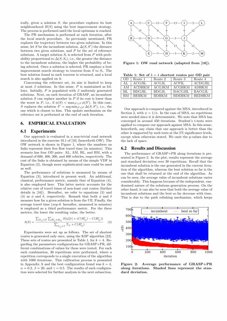
introduced in the exercise 10.1 of [16] (henceforth OW). TheOW network is shown in Figure 1, where the numbers onlinks represent their free flow travel time (in minutes). Thisscenario has four OD pairs: AL, AM, BL, and BM, with ademand of 600, 400, 300, and 400 vehicles, respectively. Thecost of the links is obtained by means of the simple VDF inEquation (2), though more sophisticated ones could be usedas well.

The performance of solutions is measured by means ofEquation (3), introduced in present work. An additional,classical, performance metric, namely that of Equation (4),is also employed here. This latter metric accounts for therelative cost of travel times of non-least cost routes (furtherdetails in [16]). Hereafter, we refer to equations (3) and(4) as φ and δ, respectively. Remark that both φ and δmeasure how far a given solution is from the UE. Finally, theaverage travel time (avg-tt hereafter, measured in minutes)is employed as a third performance metric. For the threemetrics, the lower the resulting value, the better.

δ(S) =

∑Tij∈T

∑Rr

ij∈RijS[ij][r]× (C(Rr

ij)− C(R∗ij))∑Tij∈T

Tij × C(R∗ij)(4)

Experiments were set up as follows. The set of shortestroutes is generated only once, using the KSP algorithm [23].These sets of routes are presented in Table 1, for k = 4. Re-garding the parameters configurations for GRASP+PR, dif-ferent combinations of values for these were tested. For eachsuch combination, 30 repetitions were performed, where arepetition corresponds to a single execution of the algorithmwith 1000 iterations. This calibration process is presentedin Appendix A and the best configuration found was k = 4,α = 0.2, β = 20, and γ = 0.5. The results of such configura-tion were selected for further analysis in the next subsection.

A

B

C F I L

D G J

E H K M

7

5

15

11

11

11

9

7

9

7

13

3

13

3

7

7

9

9

9

9

12

12

2

2

Figure 1: OW road network (adapted from [16]).

Table 1: Set of k = 4 shortest routes per OD pairOD Route 1 Route 2 Route 3 Route 4AL ACGJIL ACGJL ACFIL ACDGJILAM ACDHKM ACGJKM ACGHKM ADHKMBL BDGJIL BDGJL BACGJIL BACGJLBM BEHKM BDHKM BDEHKM BEDHKM

Our approach is compared against the MSA, introduced inSection 2, with ψ = 1/n. In the case of MSA, no repetitionswere needed since it is deterministic. We note that MSA hasconverged in around 450 iterations. Student’s t-tests wereapplied to compare our approach against MSA. In this sense,henceforth, any claim that one approach is better than theother is supported by such tests at the 5% significance levels,except when otherwise stated. We omit the p-values due tothe lack of space.

6.2 Results and DiscussionThe performance of GRASP+PR along iterations is pre-

sented in Figure 2. In the plot, results represent the averageand standard deviation over 30 repetitions. Recall that theincumbent solution is the one generated in the current itera-tion of the algorithm, whereas the best solution so far is theone that shall be returned at the end of the algorithm. Ascan be seen, the average value of incumbent solutions variesconsiderably. This happens because of the independent, ran-domised nature of the solutions generation process. On theother hand, it can also be seen that both the average value ofincumbent solutions and the best so far decrease with time.This is due to the path relinking mechanism, which keeps

0 200 400 600 800 1000iteration

100

200

300

400

500

600

700

Á(S

)

incumbent best so far

Figure 2: Average performance of GRASP+PRalong iterations. Shaded lines represent the stan-dard deviation.

Table 2: Performance comparison per OD pair and overallMSA GRASP+PR

OD φ δ avg-tt φ δ avg-ttAL 215 0.0001 71.21 23.37 (31.53) 0.0011 (0.002) 68.39 (0.52)AM 194 0.0032 65.74 28.60 (30.71) 0.0007 (0.001) 74.56 (0.56)BL 62 0.0020 69.35 13.87 (24.08) 0.0010 (0.002) 66.19 (0.64)BM 67 0.0001 62.13 20.17 (16.42) 0.0012 (0.001) 69.67 (0.53)Overall 538 0.0053 67.46 86.00 (32.56) 0.0039 (0.002) 69.75 (0.20)

a kind of memory by means of the reference set. In thisregard, the knowledge from previous iterations is exploitedto improve the incumbent solutions.

The comparison of our approach against MSA is shownin Table 2, in terms of φ, δ, and avg-tt . Results are pre-sented by OD pair as well as overall. In the case of GRASP,each result represents the average over 30 repetitions, thusstandard deviations are also shown (in parenthesis). Thebest results for each combination of OD pair and metric areshown in bold.

Initially, consider the overall results. It can be observedthat, on average, the solutions provided by GRASP+PRare considerably closer to the UE than those by MSA. Inother words, our assignments are fairer than those of MSA.This is due to our problem formulation, which minimises thenumber of vehicles assigned to non-least cost routes. On theother hand, the solution yielded by MSA has a lower averagetravel time. However, the point here is that our approach isconcerned with approximating the UE, not minimising theaverage travel costs. In fact, this latter is the focus of SO,not UE. The advantage of MSA in the avg-tt metric can beexplained by its structure: it works by iteratively changingthe route of a dwindling portion of the demand in order tonarrow the gap among the vehicles’ travel times. However,from the UE definition, minimising travel time per se is notthe main objective.

Now, consider the results per OD pair. Considering themetric φ, GRASP+PR clearly outperforms MSA. The rea-son here is obvious: our approach was designed to minimiseφ. In this same sense, it would be natural to expect MSAoutperforming GRASP+PR in the avg-tt metric. However,it can be seen that each algorithm outperforms the other inhalf of the cases, and the same holds for the δ metric. Forthe avg-tt metric, one can see that our approach performedbetter in the pairs going to L, whereas MSA performed bet-ter in the pairs going to M. These differences are due to thestructure of the approaches, and to the specific road net-work under consideration here. In the case of δ, however, itcan be observed that our approach fared better in the ODpairs AM and BL. Assigning routes to these two OD pairsis more difficult since all of their routes overlap in at leastone link. On the other hand, MSA presented better resultsfor the OD pairs AL and BM, whose sets of available routeshave no overlapping links between them. Thus, such resultsshow that our approach provides fairer assignments, and, atleast for the OW network, is more robust than MSA.

Regarding the avg-tt metric, some additional aspects (notshown here in their totality) can be analysed. The averagedifference between the best and worst routes of each OD pairis useful to measure the level of unfairness of an assignment.In our approach, this difference accounts for 4.38 (1.9) min-utes, whereas in MSA it accounts for 7.39 minutes. When

considering the best and worst routes over all OD pairs, inour approach this difference is of 12 (1.5) minutes, whilstin MSA it is of 22 minutes. As seen, the level of unfairnessachieved by our approach is lower than of MSA. This meansthat, compared to MSA, the level of unfairness obtained byour approach has less impact on the vehicles. Furthermore,the number of vehicles that actually suffer from such un-fairness is considerably lower in our assignments, as shownthrough the φ metric.

Summing up, the results achieved by our approach demon-strate its efficiency, fairness, and robustness to approximatethe UE of the TAP. Despite the heuristic nature of our ap-proach, it became evident that our solutions are much fairerand closer to the UE than those provided by the MSA. In-deed, the results obtained by our approach are, on average,26% (δ metric) and 84% (φ metric) better than those ofMSA. Furthermore, regarding the best solution found byour approach over all iterations, its values were only φ = 17and δ = 0.000916. Naturally, the results presented here cor-respond to the OW network and may not hold for specificroad networks. Such a fact, however, does not invalidatethe generality of our results, since the OW network presentsthe same problems of other bigger road networks, such ascongestions, routes overlapping, multiple OD pairs, etc.

7. CONCLUSIONSSolving the traffic assignment problem (TAP) is an im-

portant step towards an efficient usage of the traffic in-frastructure. In this paper, we presented the use of theGRASP+PR metaheuristic to approximate the user equi-librium (UE) of the TAP. A novel performance metric wasintroduced, which measures the amount of vehicles assignedto non-least cost routes. Through experiments, we showthat our approach outperforms the well-known method ofsuccessive averages (MSA), providing solutions that are, onaverage, significantly closer to the UE. Furthermore, our ap-proach has shown to provide assignments that are consider-ably fairer than those of MSA.

In spite of the satisfactory results achieved, there is stillspace for improvements. We have introduced a performancemetric and showed that other metrics can also be employed.An interesting approach here would be to employ a multi-objective method in order to optimise several functions atthe same time. Another interesting direction would be tomodel the UE in a disaggregate, agent-based nature. Suchdirection would lead to more realistic assignment methodsfrom the drivers’ point of view. Improving the process forgenerating the set of routes would also be useful. Someideas in this direction include: allowing a variable num-ber of routes per OD pair (or even per vehicle), and up-dating the set of routes periodically based on costs fromprevious iterations. Minor improvements include investigat-

ing other strategies for neighbourhood exploration, solutionsconstruction, and path relinking.

8. ACKNOWLEDGMENTSWe thank the reviewers for their valuable comments. The

authors are partially supported by CAPES and CNPq.

9. REFERENCES[1] A. L. C. Bazzan. Co-evolution of the dynamics in

population games: the case of traffic flow assignment.In Proc. of the 14th An. Conf. on Genetic and Evol.Comp. (companion), pages 43–50, 2012. ACM.

[2] A. L. C. Bazzan, D. Cagara, and B. Scheuermann. Anevolutionary approach to traffic assignment. In 2014IEEE Symp. on Comp. Intel. in Vehicles and Transp.Systems (CIVTS), SSCI, pages 43–50, 2014.

[3] A. L. C. Bazzan and F. Klugl. Introduction toIntelligent Systems in Traffic and Transportation.Morgan and Claypool, 2013.

[4] D. Braess, A. Nagurney, and T. Wakolbinger. On aparadox of traffic planning. Transportation Science,39(4):446–450, 2005.

[5] L. S. Buriol, M. J. Hirsh, P. M. Pardalos, T. Querido,M. G. Resende, and M. Ritt. A biased random-keygenetic algorithm for road congestion minimization.Optimization Letters, 4:619–633, 2010.

[6] D. Cagara, A. L. C. Bazzan, and B. Scheuermann.Getting you faster to work: A genetic algorithmapproach to the traffic assignment problem. In Proc. ofthe 16th GECCO (comp.), pages 105–106, 2014. ACM.

[7] H. Dia and S. Panwai. Modelling drivers’ complianceand route choice behaviour in response to travelinformation. Journal of Nonlinear Dynamics,49(4):493–509, 2007.

[8] J. C. Dias, P. Machado, D. C. Silva, and P. H. Abreu.An inverted ant colony optimization approach totraffic. Engineering Applications of ArtificialIntelligence, 36(0):122–133, 2014.

[9] T. A. Feo and M. G. Resende. A probabilistic heuristicfor a computationally difficult set covering problem.Operations Research Letters, 8(2):67–71, 1989.

[10] S. M. Galib and I. Moser. Road traffic optimisationusing an evolutionary game. In Proc. of the 13thGECCO (companion), pages 519–526, 2011. ACM.

[11] C. Gawron. Simulation-based traffic assignment. PhDthesis, University of Cologne, Cologne, Germany, 1998.

[12] F. Glover. Interfaces in Computer Science andOperations Research, chap. Tabu Search and AdaptiveMemory Programming – Advances, Applications andChallenges, pages 1–75. Springer, 1997.

[13] R. Grunitzki, G. de O. Ramos, and A. L. C. Bazzan.Individual versus difference rewards on reinforcementlearning for route choice. In 2014 Brazilian Conf. onIntelligent Systems (BRACIS), pages 253–258, 2014.

[14] V. Henn. Fuzzy route choice model for trafficassignment. Fuzzy Sets and Sys., 116(1):77–101, 2000.

[15] M. Laguna and R. Martı. Grasp and path relinking for2-layer straight line crossing minimization. INFORMSJournal on Computing, 11(1):44–52, 1999.

[16] J. Ortuzar and L. G. Willumsen. Modelling Transport.John Wiley & Sons, 3rd edition, 2001.

[17] S. Peeta and J. Yu. A hybrid model for driver routechoice incorporating en-route attributes and real-timeinformation effects. Net. and Sp. Econ., 5:21–40, 2005.

[18] A. J. Pel and A. J. Nicholson. Network effects ofpercentile-based route choice behaviour for stochastictravel times under exogenous capacity variations. InProc. of the 16th IEEE ITSC, pages 1864–1869, 2013.

[19] G. de O. Ramos and R. Grunitzki. An improvedlearning automata approach for the route choiceproblem. In Koch, Meneguzzi, and Lakkaraju, eds.,Agent Technology for Intelligent Mobile Services andSmart Societies, volume 498 of CCIS, pages 56–67.Springer, 2015.

[20] Y. Sheffi. Urban Transportation Networks: EquilibriumAnalysis With Mathematical Programming Methods.Prentice-Hall, Englewood Cliffs, USA, 1984.

[21] H. Varia, P. Gundaliya, and S. Dhingra. Applicationof genetic algorithms for joint optimization of signalsetting parameters and dynamic traffic assignment forthe real network data. Research in TransportationEconomics, 38(1):35–44, 2013.

[22] J. G. Wardrop. Some theoretical aspects of road trafficresearch. In Proceedings of the Institute of CivilEngineers, volume 2, pages 325–378, 1952.

[23] J. Y. Yen. Finding the k shortest loopless paths in anetwork. Management Science, 17(11):712–716, 1971.

APPENDIXA. PARAMETERS TUNING

Here we present a brief analysis on the values defined for theparameters involved in our approach. The test scenario is thesame as in Section 6, namely the OW network. Regarding theparameters, the following values were defined for each of them:k = {4, 10}, α = {0.2, 0.5, 0.8}, β = 20, γ = {0.2, 0.5, 0.8}. Thenumber of iterations per execution of the algorithm was set to1000 in all cases. To improve the accuracy of results, each com-bination of parameters was repeated 30 times.

The present scenario characterises a factorial experiment, wherefactors are represented by the parameters, levels by the param-eter’s values, and the response variable corresponds to the valueof solutions. In this sense, the factorial analysis of variation(ANOVA) test was employed to check for statistic equivalenceof the parameters’ values. In ANOVA, a null hypothesis is for-mulated for each factor, stating that its different levels producethe same mean response, i.e., all values of the given parameterproduce the same results on average. The alternative hypothesisis that not all levels produce the same mean response. All testshere were applied at the 5% significance levels.

The resulting p-values for factors k, α, and γ, were 2× 10−16,0.6323, and 4.6× 10−16, respectively. This means that no signif-icant differences among the values of parameter α were detected.In this sense, we adopt α = 0.2. On the other hand, the nullhypothesis was rejected for parameters k and γ. We go forwardon these factors, and apply a post-hoc test, namely the Student’st-test. Starting with parameter k, the null hypothesis is the sameas before, but with the alternative hypothesis stating that k = 4produces better solutions than k = 10. The p-value is 2.2×10−16,meaning that k = 4 is better. Indeed, the average value of solu-tions when k = 4 is 93.90± 33.09, which is much lower than the503.78 ± 59.76 of k = 10. Now, for parameter γ, we fix α = 0.2and k = 4. One test is then applied for each pair of values for γ.The resulting p-values 3.3× 10−5, 5× 10−8, and 0.1593, indicatethat, respectively, γ = 0.5 is better than γ = 0.2, γ = 0.8 is betterthan γ = 0.2, and that γ = 0.5 and γ = 0.8 are equivalent. Thus,we adopt γ = 0.5 to provide a good balance between greedy anduniform solutions.