1

An Excess-Demand Dynamic Traffic Assignment Approach for Inferring

Origin-Destination Trip Matrices

Chi Xie†

School of Naval Architecture, Ocean and Civil Engineering

Shanghai Jiaotong University

Jennifer Duthie‡

Center for Transportation Research

University of Texas at Austin

Abstract

The focus of this paper is on the development of an origin-destination (O-D) demand

estimation method for dynamic equilibrium traffic networks. It is hypothesized that

the underlying equilibrium conditions in such networks are a compromise result of

minimization of individual routing costs, minimization of traffic count matching

errors, and maximization of O-D demand entropies. By adding an upper bound of

travel demand and a dummy path with constant travel cost to each O-D pair, we

formulated the dynamic O-D demand estimation problem as an excess-demand

dynamic traffic assignment (DTA) problem defined for an expanded network with

dummy paths. Such a formulation enables us to apply existing DTA solution

methods and software tools for deriving the path flow pattern in the expanded

network and thus simultaneously obtaining the O-D demand pattern in the original

network. Following this problem transformation and network expansion strategy,

an iterative solution procedure is accordingly proposed, which resorts to repeatedly

solving the excess-demand DTA problem and adjusting the dummy path costs. An

application of the proposed modeling and solution method for an example cell-based

network problem illustrates its great promise in the methodological advance and

solution performance aspects.

1. Introduction

Dynamic traffic assignment (DTA) methods proved to be a critical analysis and

evaluation tool in many traffic network operations and planning applications. In the

past three decades, numerous contributions have been devoted to creating,

improving and implementing a variety of types of DTA methods. As a result, a

number of theoretically solid, practically operational and computationally feasible

DTA software packages emerged in recent years and have been successfully used in

the practice of traffic network analysis. During the same period, however, much less

attention has been paid to the development of origin-destination (O-D) demand

Accepted by the 4th International Symposium on Dynamic Traffic Assignment for presentation and by

Networks and Spatial Economics for publication. † Corresponding author. Professor. Address: A610 Mulan Ruth Chu Chao Bldg., 800 Dongchuan Rd.,

Shanghai 200240, China. Phone: +86 (21) 3420-8385. Fax: +86 (21) 3420-6197. E-mail:

chi.xie@sjtu.edu.cn. ‡ Research Engineer. Address: 1616 Guadalupe St., Suite 4.330, Austin, Texas 78701, United States.

Phone: +1 (512) 232-3088. Fax: +1 (512) 232-3153. E-mail: jduthie@mail.utexas.edu.

2

estimation methods for dynamic networks. Many existing methods are not

inherently consistent with the underlying dynamic routing behavior and are often

specific to only a certain type of network environments or a certain category of field

data. In many cases, lack of reliable dynamic O-D demand estimation methods

seriously impedes the application of DTA tools.

Among different data sources, traffic data provided by traffic sensors are believed to

be the most readily available, frequently updated, and qualitatively accurate.

Because of this reason, traffic data-based demand estimation methods are often

preferable to other methods relying on alternative data sources, from the perspective

of cost effectiveness. The general design philosophy for such demand estimation

methods is to make it, when the estimated demand table is used as input to evaluate

dynamic network flows, to achieve the goal of replicating or approximating the

observed traffic data in a maximum and unbiased manner. Given that a dynamic O-

D demand table is represented as a consecutive time series of O-D matrices, the

replication or approximation is often achieved by some statistical optimization

principles. On the other hand, to properly reflect individual travel behaviors and

the network congestion effect, the flow-cost consistency should be explicitly or

implicitly implied in the demand estimation process. Characterizing the network

equilibrium imposed by traffic dynamics and travel behaviors in general requires a

DTA model. Simultaneously accommodating both the optimization principles and

dynamic equilibrium conditions in a single model poses a very challenging modeling

task.

Our focus in this paper is on the development of a dynamic O-D demand estimation

method that uses traffic counts as input data and is applicable to general traffic

networks while ensuring an endogenous time-dependent flow-cost consistency and

realizing a simultaneous determination of all time-dependent O-D matrices over the

analysis period. In the existing literature, two model structures for this type of

problems were proposed: 1) optimization model with equilibrium constraints, which

typically forms the so-called bi-level mathematical programming structure, where

the lower-level problem is used to specify the equilibrium network flows; 2)

composite equilibrium model, which poses a single-level equilibrium problem where

the equilibrium costs are a composite result of actual travel costs and artificial

optimality terms corresponding to some given statistical optimization principle.

Different model structures led to different solution methods in the literature.

Specifically, in the bi-level case, Tavana (2001) applied an iterative optimization-

assignment procedure to approximate an O-D demand table by repeatedly tackling

the upper-level optimization problem that includes a term of minimizing the

estimation deviation from an available historical O-D matrix and the lower-level

assignment problem that represents the dynamic network flows. Cipriani et al.

(2011) also employed an iterative optimization-assignment solution framework, in

which an approximate gradient-based method is used to search for the improvement

direction of the objective function. Zhou et al. (2012) converted their bi-level

problem into a one-level problem by Lagrangian relaxation, in which the lower-level

problem specified by a gap function is relaxed, and resorted to a solution approach of

iteratively solving the relaxed problem and updating the Lagrangian multipliers.

Mahut et al. (2004) implemented a trip table adjustment method with the aim of

3

minimizing the difference between measured intersection counts and simulated

turning movements using a steepest descent method. This optimization principle

and method were originally proposed by Spiess (1990) for a static O-D demand

estimation problem, who attempted to find a solution that minimizes the sum of

squared deviations between assigned and observed flows at a local optimum while

maintaining the demand change across O-D pairs close to the initial O-D demand

matrix in a proportional way. Choi et al. (2009) also adopted Speiss’ method, which

starts with an O-D matrix distributed uniformly over time, finding the first locally

optimal solution that minimizes the sum of squared flow deviations. In view of the

solution difficulty caused by the bi-level structure, metaheuristic methods have been

used for searching for optimal O-D demand matrices, for example, the evolutionary

algorithm employed by Kattan and Abdulhai (2006). It is noted that in all these

mentioned dynamic O-D demand estimation studies, a simulation-based DTA model

is used to estimate dynamic network flows.

In the single-level case, the earliest work is due to Bell et al. (1997), to the author’s

best knowledge. They formulated a composite equilibrium model in the context of

capacitated stochastic traffic assignment, which accounts for the routing behavior of

simultaneously minimizing the perceived individual travel costs (including

undelayed travel time and queuing delay) and dual costs related to measured link

counts. However, their model presumes accurate traffic measurements and cannot

deal with the traffic count inconsistency issue. The single-level composite

equilibrium modeling approach has been also employed in other O-D demand

estimation problems, for either static or dynamic networks, including Nie and Zhang

(2008, 2010), Shen and Wynter (2011), and Xie and Kockelman (2012), with different

behavioral assumptions and modeling components from one another. Evidently, in

terms of the solution tractability and computational efficiency, the single-level

approach is preferable to the bi-level.

The literature also contains various other dynamic O-D demand estimation methods

for alternative network settings and circumstances, for example, those for

intersections or highway corridors, those using an exogenous dynamic assignment

matrix, and those for real-time demand estimations and predictions. For a

comprehensive review on dynamic O-D demand estimation methods, interested

readers are referred to a few recent Ph.D. dissertations, including Tavana (2001),

Zhou (2004), and Nie (2006).

The remaining part of this paper is organized in the following order. In Section 2,

we introduce the notation used throughout the paper, the basic modeling mechanism

and dicretization scheme of network flow models, and the methods of evaluating

path travel times, least-squares path deviation costs and maximum-entropy path

deviation costs. We employ the cell transmission model (CTM) to describe the traffic

propagation and interaction over the network, due to its numerical consistency with

the classic hydrodynamic traffic flow theory and its extensive use in various dynamic

network equilibrium and optimization applications. In Section 3, we define the

optimality conditions of the proposed augmented DTA problem and formulate the

problem into a variational inequality (VI) model and prove its solution existence,

equivalence and uniqueness. Section 4 presents an iterative solution procedure, of

which the major algorithmic steps include solving the augmented DTA problem and

4

adjusting the dummy path costs. Section 5 illustrates the application of the

modeling and solution methods through a numerical example and discusses the

issues of large-scale implementations. Finally, Section 6 concludes the paper.

2. Preliminaries

2.1. Notation

The notation list below defines all the sets, parameters and variables used through

the paper.

Sets

Set of cells

Set of cell links

Set of origin cells

Set of destination cells

Set of cell links on which traffic counts are measured

Set of origin cells of which the downstream cell links where traffic counts

are measured

Set of destination cells of which the upstream cell links where traffic counts

are measured

Set of downstream cells of cell

Set of upstream cells of cell

Set of paths

Set of paths connecting O-D pair -

Set of time intervals

Set of demand departure intervals in demand estimation interval

Set of traffic movement intervals in traffic measurement interval

Parameters

Duration of demand departure interval , where and Duration of traffic movement interval , where and Duration of demand estimation interval , where and is a

positive integer

Duration of traffic measurement interval , where and is a

positive integer

Free-flow speed of cell Backward shockwave speed of cell Maximum number of vehicles (or holding capacity) that can be held in cell

in traffic movement interval

Maximum amount of flows (or flow capacity) going through cell link ( ) in

traffic movement interval

Inclusion indicator of demand departure interval in demand estimation

interval , where if , and otherwise

Inclusion indicator of traffic movement interval in traffic measurement

interval , where if , and otherwise

5

Weighting coefficient of link flow deviations

Weighting coefficient of link flow deviations

Weighting coefficient of link flow deviations

Weighting coefficient of O-D flow entropies

Observed traffic counts going through cell link ( ) in traffic measurement

interval

Observed traffic counts going through the cordon for origin in traffic

measurement interval

Observed traffic counts going through the cordon for destination in traffic

measurement interval

Variables

Traffic flow departing in demand departure interval and traveling along

path from origin to destination

Traffic flow departing in demand estimation interval and traveling along

path from origin to destination , where ∑

Travel demand departing in demand departure interval from origin to

destination , where ∑

Travel demand departing in demand estimation interval from origin to

destination , where

and ∑

Excess travel demand departing in demand departure interval along the

dummy path from origin to destination

Traffic flow going through cell link ( ) in traffic movement interval

Traffic flow going through cell link ( ) in traffic measurement interval ,

where ∑

Number of vehicles in cell in traffic movement interval

Proportion of path flow

going through cell link ( ) in traffic movement

interval

Proportion of path flow

going through cell link ( ) in traffic

measurement interval , where ∑

Travel time of traffic flow departing in demand departure interval and

traveling along path from origin to destination

Travel cost of traffic flow departing in demand departure interval and

traveling along path from origin to destination

Deviation cost of traffic flow departing in demand departure interval and

traveling along path from origin to destination

Entropy cost of traffic flow departing in demand departure interval and

traveling along path from origin to destination

Minimum travel cost of traffic flow departing in demand departure interval

and traveling along all paths from origin to destination in the original network

Given travel cost of traffic flow departing in demand departure interval

and traveling along the dummy path from origin to destination

Minimum travel cost of traffic flow departing in demand departure interval

and traveling along all paths from origin to destination in the expanded

network

6

Deviation of link flow between its estimated and observed values

Deviation of sum of link flows ∑ departing from origin

between its estimated and observed values

Deviation of sum of link flows ∑ arriving at destination

between its estimated and observed values

2.2. Cell transmission model and cell-based network

It is well known that the CTM theory proposed by Daganzo (1994, 1995) offers a

discrete approximation to the classic hydrodynamic traffic flow model of Lighthill

and Whitham (1955) and Richards (1956). According to the theory, any roadway in

a network is discretized into a series of homogeneous cells and time discretized into

a set of equal intervals such that the cell length is equal to the distance traveled in

one time interval by traffic at the free-flow speed. Cell links (or cell connectors) are

constructed to connect adjacent cells along roadways and at junctions/intersections.

Both cells and cell links are directional, as consistent with the given traffic

directions. Any path in a cell-based network is represented by a series of

consecutive cells with the same traffic direction, along which the most upstream cell

is its origin cell and the most downstream cell is its destination cell.

Let us use ( ) to represent a cell-based, time-sliced network, where , and

are the sets of cells, cell links and time intervals, respectively. The sets of origin

cells and destination cells, and , are two special subsets of , i.e., and . The time intervals we refer to here include two types of intervals, namely, the

demand departure intervals and traffic movement intervals ; in our case,

the two types of intervals are equivalent. It should be noted that the demand

departure interval and traffic movement interval are different from the demand

estimation interval and traffic measurement interval, as we will introduce later on.

For now, let us emphasize that in the text hereafter, unless specified, any time

interval we refer to means a demand departure interval, a traffic movement

interval, or both of them, depending on which specification is the most appropriate.

The spatiotemporal relationship of traffic flow variables in a cell-based network can

be specified by the following set of recursive equations along traffic directions:

∑

∑

( ), (1.1)

{ ∑

(

) ∑

}

( ) , (1.2)

Note that the above set of equations synthetically accommodates the traffic flow

conservation and propagation conditions in all the cases, including the linear,

merging and diverging cases. The special cases are for origin and destination cells,

7

which represent the boundary of the network (i.e., origin cells do not have upstream

cells and destination cells do not have downstream cells) and are set with an infinite

capacity (i.e., , and

, ). Following this special

treatment, the flow conservation equation for origin cells and destination cells can

be simplified into the following reduced forms:

∑

∑

, , (2.1)

∑

, (2.2)

where in the first equation above, is the travel demand from origin cell to

destination cell departing in the demand departure interval , and it is noted that

in this equation, the indexes of the demand departure interval and the traffic

movement interval coincide, i.e., .

It should be noted that the above flow conservation equations (i.e., (1.1), (2.1) and

(2.2)) are given on the cell level, which aggregate traffic flows from all relevant

paths. For each path connecting O-D pair - and demand departure interval , a

series of similar time-dependent path-specific flow conservation equations to the

above still hold, as shown below,

, , , , , (3.1)

, , , , (3.2)

, , , , (3.3)

where, by definition, denotes the number of vehicles along path departing

during demand departure interval and arriving at cell during traffic movement

interval ,

represents the traffic flow along path departing

during demand departure interval and going through cell link ( ) during traffic

movement interval , and is the path flow along path departing during

demand departure interval , respectively. The above three flow conservation

functions are applicable to ordinary, origin and destination cells, respectively. Note

here that for any cell along a particular path, there is at most one single upstream

cell and one single downstream cell.

Since its invention, CTM has been extensively used for modeling and solving various

dynamic network equilibrium and optimization problems, such as traffic assignment

(Ziliaskopoulos, 2000; Lo and Szeto, 2002), network design (Waller et al., 2006;

Ukkusuri and Waller, 2008; Chung et al., 2011), signal control (Lo, 2001;

Karoonsoontawong and Waller, 2010), and evacuation planning (Chiu and Zheng,

2007; Yao et al., 2009; Xie et al., 2010b), to just name a few. Needless to say,

8

modeling and solving all these dynamic network problems requires time-dependent

travel demand matrices for cell-based networks. The inherent discrete location and

time settings within cell-based networks provides a natural discretization scheme

for modeling discrete dynamic traffic systems.

2.3. Discrete settings of cell-based networks

By definition, the traffic state (characterized by traffic variables) in any cell or cell

link during any single time interval is time-invariant. Following the time

discretization scheme, time-varying networks with continuous spatial and temporal

variations are approximated by a series of discrete time-invariant network states.

To reflect traffic dynamics with a satisfactorily high precision, the duration of time

intervals is typically set to several seconds. The length of cells is then determined in

terms of the discretization rule required by the CTM theory, as described above.

Other two types of intervals, namely, demand estimation interval and traffic

measurement interval, are often used in dynamic O-D demand estimation problems,

because of some engineering reasons in practice. Demand estimation intervals are

the time intervals for which O-D demands are assumed to be time-invariant or

stable. The duration of a demand estimation interval is typically set as 10 to 30

minutes, depending on the desired modeling fidelity. Typically, the duration should

not be too short to smooth random demand fluctuations. Traffic measurement

intervals specify the frequency at which traffic sensors aggregate and report traffic

states. The duration of traffic measurement intervals often falls into a range of 15

to 60 minutes. For modeling convenience, we set the duration of a demand

estimation interval to be an integer number of times the duration of a demand

departure interval and set the duration of a traffic measurement interval to be an

integer number of times the duration of a traffic movement interval, i.e.,

∑

(4.1)

∑

(4.2)

where and are the number of demand departure intervals in a demand

estimation interval and the number of traffic movement intervals in a traffic

measurement interval, respectively.

These different time intervals discussed above are used for different system

modeling precision requirements. Specifically, traffic dynamics are modeled on a

relatively precise level of several seconds, specified by the demand departure

interval and traffic movement interval, while O-D demand variations are estimated

and traffic flow variations are observed on a relatively coarse level, respectively, of

roughly several to tens of minutes and tens of minutes to several hours. A similar

scheme of using mixed time intervals is employed by, for example, Nie and Zhang

(2008) and Zhou et al. (2012) in their dynamic O-D demand estimation models.

9

Given the above discrete network settings, we are now ready for further specifying

the inherent time-dependent relationships among all traffic flow and demand

variables defined at different time scales. First, by flow conservation, the path flows

and O-D demand for any O-D pair - in each demand departure interval has the

following summation relationship:

∑

, , (5)

where, by definition,

⁄ . The incidence relationship between the link flow

in traffic movement interval and the path flow departing in demand departure

interval is expressed as,

∑∑∑

( ), (6)

where denotes the proportion of path flow

contributing to link flow ,

i.e., the proportion of path flow departing in demand departure interval going

through cell link ( ) in traffic movement interval . By definition, we know that

. It is worth mentioning here that a complete set of

and

information over the whole network and across all time intervals specifies the entire

dynamic network flow pattern. As we will see, the path flow pattern [ ] is a

result of route choices and the path flow proportion pattern [ ] is

determined by the traffic propagation and interaction, which is often characterized

as a dynamic network loading (DNL) process. Furthermore, given ∑ ,

the above path-link relationship can be extended as,

∑∑∑

( ), (7)

where ∑

denotes the proportion of path flow contributing to

link flow , where . As we will see, this extended path-link

relationship is needed in calculating the flow deviations between the observed and

estimated link flows.

Finally, for a complete specification of the feasible region, the flow nonnegativity

constraint is always required:

, , , (8)

2.4. Evaluation of path travel times

10

It is well known that the relationship between traffic flows and travel times, or the

travel time function, is the key performance indicator of evaluating the supply

performance of network components and determining the route choice pattern. For

most dynamic traffic networks, there exists no explicit analytical travel time

function; the cell-based network is not an exclusive case. Given the path choice

pattern over the network, evaluating path travel times typically requires invoking a

numerical DNL process.

A DNL process and a path travel time evaluation procedure for cell-based networks

are well described in Daganzo (1995) and Lo and Szeto (2002). The following text

only presents the most essential information and result. The central scheme of the

path travel time evaluation procedure for cell-based networks is based on the use of

the cumulative departure path flows from origin cells and the cumulative arrival

flows at destination cells. Let denote the cumulative traffic flow departing from

origin cell along path before the end of departure demand interval and the

cumulative flow arriving at destination cell along path before the end of traffic

movement interval :

∑

, , , (9.1)

∑

, , , (9.2)

where ( ) is the last cell link adjacent to destination cell along path . Note that

given the path flow pattern [ ] and the DNL process,

and are the

functions of time interval and time interval , respectively. For discussion

convenience, we write these two functions as

( ) and

( ). Then

let ( ) and (

) be the inverse functions of and

, i.e., ( ) (

)

and ( ) (

). The (average) path travel time of path flow

departing

during demand departure interval can then be calculated as,

∫ [( ) ( ) (

) ( )]

, , , (10)

where, by definition,

is the path flow along path connecting O-D

pair - , departing in demand departure interval . If path flow equals zero, its

corresponding path travel time becomes (

) ( ) (

) ( ),

which is apparently an integer number of times the time interval.

The following property of the defined path travel time is required to ensure the

solution existence of the O-D demand estimation model proposed in the next section.

2.5. Path deviation cost term for least squares

11

As we stated earlier, one of the optimization criteria with the defined O-D demand

estimation problem is to minimize the difference between the observed traffic counts

and their estimated values. In our case, the observed traffic counts include link

counts and cordon counts. Such traffic counts can be collected by a variety of

pavement-embedded or roadside traffic sensors. In an aggregate form, this

minimization principle can be represented by a weighted sum of least squares of the

deviations of all observed and estimated traffic counts over the network:

∑ ∑( )

( )

∑∑( )

∑∑( )

(11.1)

where , , and are defined as,

∑∑∑

( ) , (11.2)

∑ ∑∑∑

, (11.3)

∑ ∑∑∑

, (11.4)

It is noted that each of these least-squares terms is of a special form of the

generalized least-squares estimator (see Cascetta et al., 1993), in which the special

setting is that the variance-covariance matrix is a scalar matrix with its diagonal

entry equal to ⁄ , ⁄ , or ⁄ . The variance-covariance matrix contains

important statistical flow dependence information between locations where traffic

flows are measured. However, very often, the variance-covariance matrix is difficult

to estimate due to data inadequacy, if not impossible. This is also true in our case,

so we use the least-squares instead of generalized least-squares estimator.

Combined together, these least-squares components in the deviation minimization

function will appear in the optimality conditions as the following path deviation cost

term:

∑ ∑

( )

∑

∑

12

, , , (12)

It is noted that the weighting coefficients , and play a projection operation

role, in that they project flow deviations , and to the cost deviation

.

2.6. Path entropy cost term for maximum entropy

In addition to the objective of matching traffic measurements, entropy maximization

is another fundamental optimization principle included in our model for specifying

the primitive nature of the spatial distribution of O-D demands. Wilson (1967, 1969,

1970) first justify the usefulness of entropy maximization in a number of travel

demand analysis problems, such as trip distribution, mode split, and route split.

Anas (1983) proved the equivalence of the aggregate-level entropy maximization

theory and the disaggregate-level utility maximization theory (in the case of the

multinomial logit model) in the context of O-D demand distribution. The maximum-

entropy principle has been frequently used for various O-D demand estimation

problems, when no historical or reference O-D demand matrix is available (see, for

example, Van Zuylen and Willumsen, 1980; Willumsen, 1981, 1984; Xie et al.,

2010a). Following Willumsen (1984), the maximum-entropy function of O-D

demands over a dynamic traffic network can be written as,

∑∑[

( )]

(13.1)

or

∑∑[ (

) ]

(13.2)

where

∑∑

, , (13.3)

Further, similar to Xie et al. (2010a, 2011), we may accordingly introduce a

corresponding path entropy cost term in the optimality conditions to the above

maximum-entropy function, which can be obtained by deriving its first-order

derivative with respect to path flow :

∑ ( )

, , , (14)

13

It is clear that by definition this path entropy cost term implies a certain level

of spatial and temporal homogeneity, in that its value is common to all path flows

traveling from origin to destination and departing during demand estimation

interval . This result implies the condition that introducing the entropy cost term

into the desired optimality conditions does not change the path cost difference

between any pair of path flows connecting the same O-D pair and departing in the

same departure interval, and hence not alter the route choice results and

equilibrium conditions associated with this O-D pair, if compared to the network

equilibrium solution without adding the path entropy cost term. However, the

entropy cost term in general does differ between different O-D pairs.

3. An excess-demand dynamic traffic assignment problem

Given all the required modeling elements in the last section, we are now ready for

discussing an excess-demand network modeling framework, by which the proposed

dynamic O-D demand estimation problem can be solved by repeatedly solving a DTA

problem for an expanded network with excess demands on dummy paths. The

optimality conditions implied by this DTA problem are a compromise result of the

minimization of individual travel times, minimization of traffic count deviations, and

maximization of O-D demand entropies. We first derive its optimality conditions

starting from the prime definition of the widely accepted dynamic user equilibrium

(DUE) conditions.

3.1. Optimality conditions

Ideally, the DUE conditions should be implied in the solution of an O-D demand

estimation problem. In general, this set of conditions can be characterized by the

following nonlinear complementarity system (see Friesz et al., 1993; Smith, 1993; Lo

and Szeto, 2002):

{

(

)

, , , (15)

where

satisfies the constraint set (3)-(8),

is defined in (10), and is the

minimum of all relevant path times, i.e.,

{

} , , (16)

To distinguish it from our alternative equilibrium conditions defined later on, we

term the above equilibrium conditions the ideal dynamic user equilibrium (IDUE),

in which all path travel costs only consist of path travel times.

By taking into account the path deviation cost (resulted from the least-squares

objective) and the path entropy cost (resulted from the maximum-entropy objective),

14

an augmented equilibrium flow pattern may be formed, which represents a

compromise result between prompting the IDUE conditions and achieving the stated

least-squares and maximum-entropy objectives. Interested readers may refer to Nie

and Zhang (2008, 2010), Shen and Wynter (2011), and Xie and Kockelman (2012) for

conceptually similar ideas for static and dynamic networks. We use the augmented

dynamic user equilibrium (ADUE) conditions to term this equilibrium case. Its

corresponding complementarity system is,

{

(

)

, , , (17)

where the path deviation cost

and path entropy cost

follow the previous

definitions in (12) and (14). Note that the path entropy cost is common to all paths

connecting the same O-D pair and departing in the same demand departure

interval.

It is also noted that when

, we have

, which implies

that the ADUE closely approaches an alternative DUE, under which the path costs

evaluated by individual travelers for route choice comprise travel times only.

Compared to the IDUE defined in (15), this alternative DUE merely contains an

additional common path cost

. Apparently, adding this common path cost does

not change the route choice result.

Now let us set as,

, , , (18)

and accordingly name the augmented path travel cost. Following this definition,

the ADUE presented above can be described as: Among the set of paths connecting

the same O-D pair, for the same demand departure interval, all paths carrying a

positive flow have an equal augmented travel cost and any path with a higher

augmented travel cost carries no flow. The remaining work is then to construct a

proper model that can be used to derive the solution corresponding to the augmented

equilibrium conditions and establish its usefulness for the defined O-D demand

estimation problem.

According to Lagrangian relaxation theory, we know that the existence of the

minimum augmented path travel cost (or the augmented O-D travel cost) in the

equilibrium conditions implies that a constant O-D demand (or an O-D demand

function) must be given as input. This requirement, however, conflicts with the

fact that is a decision variable to be estimated in the proposed O-D estimation

problem, which is neither a constant nor a closed-form function of travel costs. To

relax this conflict, we employ a problem transformation and network expansion

strategy, which comprises two operations: 1) assume the existence of a maximum O-

15

D flow for each O-D pair - and each demand departure interval ; 2) add a

dummy path directly connecting each O-D pair - to the network, as shown in

Figure 1, and assume that the travel cost along this dummy path for each demand

departure interval , , is known a priori. It should be noted here that the given

maximum O-D flow here is a sufficiently large constant. By sufficiently large,

we mean that , , , , is larger than what is needed to fully ensure

over the whole network; otherwise, it might result in

, where

{ {

}

}. In the expanded network with dummy paths, the proposed

dynamic O-D estimation problem is transformed to a DTA problem that embraces

the augmented equilibrium conditions defined above.

Figure 1 Network expansion by adding dummy paths to connect O-D pairs

Following the conventional terminology fashion (see Sheffi, 1985, for example), we

call the travel demand going through the dummy path the excess demand of O-D

pair - . In accordance, the augmented DTA problem is named the excess-demand

DTA problem. Given the upper bound of travel demand for each O-D pair, ,

the following flow conservation relationship applies to the excess-demand DTA

problem,

, , (19)

where ∑

and

are the O-D demand to be estimated and the excess

demand of O-D pair - during demand departure interval , respectively. Following

this problem transformation, we can see that the original dynamic O-D estimation

problem can now be solved by equivalently solving the excess-demand DTA problem,

if a set of proper augmented O-D travel costs for all O-D pairs and all demand

departure intervals are supplied.

The following text formally defines the excess-demand DTA problem for the

expanded network and states its solution equivalence to the desired optimality

conditions, i.e., the ADUE conditions.

r s

Dummy path

16

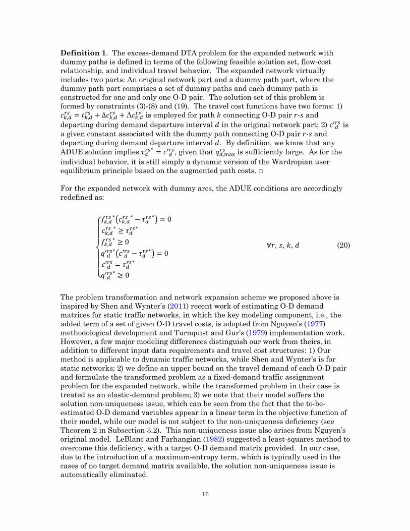
Definition 1. The excess-demand DTA problem for the expanded network with

dummy paths is defined in terms of the following feasible solution set, flow-cost

relationship, and individual travel behavior. The expanded network virtually

includes two parts: An original network part and a dummy path part, where the

dummy path part comprises a set of dummy paths and each dummy path is

constructed for one and only one O-D pair. The solution set of this problem is

formed by constraints (3)-(8) and (19). The travel cost functions have two forms: 1)

is employed for path connecting O-D pair - and

departing during demand departure interval in the original network part; 2) is

a given constant associated with the dummy path connecting O-D pair - and

departing during demand departure interval . By definition, we know that any

ADUE solution implies

, given that is sufficiently large. As for the

individual behavior, it is still simply a dynamic version of the Wardropian user

equilibrium principle based on the augmented path costs. □

For the expanded network with dummy arcs, the ADUE conditions are accordingly

redefined as:

{

(

)

(

)

, , , (20)

The problem transformation and network expansion scheme we proposed above is

inspired by Shen and Wynter’s (2011) recent work of estimating O-D demand

matrices for static traffic networks, in which the key modeling component, i.e., the

added term of a set of given O-D travel costs, is adopted from Nguyen’s (1977)

methodological development and Turnquist and Gur’s (1979) implementation work.

However, a few major modeling differences distinguish our work from theirs, in

addition to different input data requirements and travel cost structures: 1) Our

method is applicable to dynamic traffic networks, while Shen and Wynter’s is for

static networks; 2) we define an upper bound on the travel demand of each O-D pair

and formulate the transformed problem as a fixed-demand traffic assignment

problem for the expanded network, while the transformed problem in their case is

treated as an elastic-demand problem; 3) we note that their model suffers the

solution non-uniqueness issue, which can be seen from the fact that the to-be-

estimated O-D demand variables appear in a linear term in the objective function of

their model, while our model is not subject to the non-uniqueness deficiency (see

Theorem 2 in Subsection 3.2). This non-uniqueness issue also arises from Nguyen’s

original model. LeBlanc and Farhangian (1982) suggested a least-squares method to

overcome this deficiency, with a target O-D demand matrix provided. In our case,

due to the introduction of a maximum-entropy term, which is typically used in the

cases of no target demand matrix available, the solution non-uniqueness issue is

automatically eliminated.

17

3.2. A variational inequality formulation

Given the inherent asymmetry and nonadditivity of travel time functions, the

excess-demand DTA problem in general cannot be written into an optimization

formulation. Therefore, we resort to a VI model to characterize the problem’s

equilibrium conditions suggested above. Of course, VI is not the only modeling

choice; other general equilibrium modeling techniques, such as nonlinear

complementarity problems, fixed-point problems, or gap (or merit) function-based

optimization problems, can be potentially used for constructing an appropriate

model here (see Facchinei and Pang, 2003).

The proposed VI model is expressed as: For all ( ) , where [ ], [

],

and is the feasible solution set confined by constraints (3)-(8) and (19), find

( ) such that

∑∑[∑

(

)

(

)]

(21)

where

is the equilibrium augmented travel cost of path

connecting O-D pair - in the original network part for demand departure

interval , and is the given travel cost of the dummy path connecting O-D pair -

for demand departure interval .

Note that in the ideal traffic count matching case (i.e., all

values approach

zero), a proper value of should be the sum of

{

}

, where

is a function of or

(shown in (14)). While may be collected by probe

vehicles, license plate recognition techniques, or electronic toll collection systems,

is difficult to measure. After all, itself is the to-be-estimated variable of the

model. Due to this reason, an estimation method is required to determine the

value. This task will be accomplished in the next section. The remaining text in

this section proves the proposed VI model’s solution equivalence to the ADUE

conditions defined in (20).

Theorem 1. A path flow pattern ( ) , where [

] and [ ],

solves the VI problem in (21), if and only if ( ) satisfies the ADUE conditions

defined in (20).

Proof. We first establish the sufficiency. If satisfies the ADUE conditions, it can

be characterized by,

{

, , ,

18

Similarly, can be characterized by the above complementarity system as well.

Now suppose that we have another feasible solution ( ) . It is readily seen

that the following inequality holds by comparing the total cost between ( ) and ( ) for O-D pair - ,

∑

∑

, ,

∑

(

)

(

) , ,

since the

is the lowest path cost among all the paths (including the

dummy path) connecting O-D pair - for demand departure interval . Summing

up the above inequality associated with each O-D pair and time interval results in

the VI problem in (21).

We then establish the necessity. Suppose that ( ) is a solution of the VI

problem, but it does not satisfy the ADUE conditions. The latter assumption means

that for some path connecting O-D pair - and departing demand departure

interval , the following condition appears:

{

The same assumption can be applied to the dummy path connecting each O-D pair.

Let us reassign path flow

from path to another path with its cost equal to

and denote the resulting new path flow pattern ( ). Because

as well

as

, , , , , and

, , , (or

, , , , , and

, , , ), the following inequality holds,

∑∑[∑

]

∑∑[∑

]

which contradicts with the inequality of the VI problem. □

4. An iterative solution procedure

On the basis of the problem transformation and network expansion strategy, it is

now clear that our solution approach for solving the dynamic O-D demand

estimation problem involves two major algorithmic steps: 1) finding a proper set of

dummy path costs ; 2) solving the excess-demand DTA problem in the expanded

network. The section elaborates these algorithmic developments.

19

4.1. An iterative combinatorial algorithm for inferring dynamic network flows

Note that the excess-demand DTA problem presented in (21) is simply an ordinary

DTA problem for cell-based networks except that the path costs of its dummy paths

are given as constants and the path costs of its real paths comprise of travel times,

traffic count deviations, and demand entropies. The fix of constant path costs can be

implemented by setting the free-flow travel time along the dummy path equal to the

given constant and setting its capacity to infinity. To accommodate the time

dependence of the path cost of each dummy path, the only extra modeling

requirement is to allow its free-flow travel time to be time-dependent. Moreover, in

a cell-based network, if the adjustment of the dummy path’s free-flow travel time is

implemented by adding or removing a number of cells along the dummy path, the

excess-demand DTA problem can be solved by any existing solver for cell-based

dynamic networks.

Nevertheless, the excess-demand DTA problem can be solved by a number of

different solution methods, including conventional relaxation methods, projection

methods and their variants, which can all be described as an iterative convergent

optimization procedure, and combinatorial optimization methods, which assign

individual vehicles in a discrete manner.

Our particular interest is given to a combinatorial optimization method, which was

recently proposed by Waller and Ziliaskopoulos (2006) for single-destination DTA

problems and extended by Golani and Waller (2004) for general multi-destination

problems. Following the assumption that on any arc the travel time experienced by

a given vehicle is not affected by any vehicle behind it, the single-destination

combinatorial method achieves the equilibrium by assigning vehicles individually

into the network in the time order by a time-dependent shortest path algorithm and

simultaneously reducing the capacity of all cells and cell links occupied by assigned

vehicles. The multi-destination version employs a Gauss-Seidel decomposition

scheme to sequentially compute the equilibrium flow pattern for each destination.

The time-dependent shortest path algorithm is the core algorithmic step of the

combinatorial methods. While the single-destination procedure guarantees the

optimality of the traffic assignment solution (if the tiny rounding error introduced by

the discrete assignment is ignored), the multi-destination procedure is merely an

approximate algorithm, since it may not guarantee the first-in-first-out (FIFO) order

through the network between vehicles destined to different destinations. Given the

discrete nature of the combinatorial optimization method, its solution is an

approximation to the naturally continuous flow solution of the CTM model.

As a generalization to the work by Waller and Ziliaskopoulos (2006), we developed a

similar combinatorial optimization method for multi-destination DTA problems.

This method poses an exact solution procedure for a certain type of acyclic network

topologies and an approximate procedure for general network topologies. The

following text gives a brief description of its essential features and explains how it is

applied to the DTA problem defined in this paper.

Different from the all-to-one shortest path algorithm used in the single-destination

method, the core algorithmic procedure of our multi-destination method is an all-to-

20

all shortest-earliest path algorithm. This algorithm finds one or more shortest-

earliest paths, each of which is not only the shortest one among all paths connecting

the same O-D pair, but also the one arriving at any common node earliest among all

paths over the network. The key operation for the latter requirement is to compare

the arrival times of individual vehicles from different origins to different

destinations at each merging node and only assign those vehicles into the network

which arrive at each of their passing nodes earlier than any other potential arriving

vehicles. The optimal solutions of multi-destination DTA problems are ensured by

this shortest-earliest path algorithm for acyclic networks. Though the acyclic

requirement seems a very strict assumption, the resulting exact combinatorial

method is still applicable to general traffic networks with topological cycles, if some

preliminary path selection or elimination procedure is used to remove cycles for each

O-D pair prior to the execution of the shortest-earliest path algorithm.

In our case, an added algorithmic task for solving the proposed excess-demand DTA

problem is to take into account traffic count deviations in the shortest-earliest path

search process. Recall that the travel costs of the defined DTA problem comprise

travel times, traffic count deviations, and demand entropies (see Subsections 2.4, 2.5

and 2.6). The entropy cost is common to all paths connecting a single O-D pair, so

its value does not impact path choices. We are only concerned about path travel

times and path deviation costs in the path search. Note that travel times are

evaluated for roadway segments in terms of individual traffic movements, while

traffic count deviations are aggregated flow evaluation results at some roadway

points. As a result, path deviation costs affect individual path choices, but not the

order of individual vehicles moving in the traffic stream. The simultaneous

consideration of travel times and deviation costs results in a more sophisticated path

search process for the defined DTA problem. In particular, each time of performing

the dynamic programming operations in the all-to-all shortest-earliest path search,

the path arriving at a merging node with the lowest sum of travel time and

deviation cost should be selected among all paths connecting the same O-D pair; for

paths connecting different O-D pairs, the path arriving at a merging node in the

earliest time should be selected. Such operations form a two-step algorithmic

process.

Moreover, according to its definition, we know that the path deviation cost can be

numerically evaluated only after the network flows are assigned (refer to (12)).

Because of this reason, the one-time combinatorial method, which is designed for

DTA problems in terms of travel times only, cannot be directly applied for solving

the defined DTA problem in this paper, but merely serves as a subroutine in a more

general DTA solution framework—the method of successive averages (MSA).

Given that the MSA procedure is an iterative convergent process, embedding the

combinatorial method into this iterative solution framework results in an iterative

combinatorial optimization procedure. Its major algorithmic steps can be sketched

as follows:

21

Step 0: Solve the defined excess-demand DTA problem with all by the

combinatorial method. Calculate ( )

in terms of ( )

, ( )

, ( )

, and ( )

. Set

.

Step 1: Solve the defined DTA problem with ( )

, which generates a network flow

pattern ( )

, ( )

, ( )

, and ( )

.

Step 2: Find the new network flow pattern by setting ( ) ( )

( )

( )

, ( )

( ) ( )

( )

, ( )

( ) ( )

( )

, and ( )

( ) ( )

( )

.

Step 3: Update ( )

in terms of ( )

, ( )

, ( )

, and ( )

.

Step 4: If solution convergence is obtained, stop the procedure; otherwise, set

and go to step 1.

It is noted that the above MSA procedure employs a fixed step size . In our

numerical experiment below, 0.5 is used.

4.2. An iterative heuristic for determining dummy path costs

The remaining algorithmic concern is on the derivation of an appropriate set of time-

dependent costs of dummy paths. An iterative heuristic procedure similar to Shen

and Wynter (2011) is sketched below for this purpose.

Step 0: Initialize ( ) by setting it to be an overestimated value of

, i.e.,

( )

, , , , where denotes the dummy path cost for O-D pair - and

demand departure interval corresponding to the optimal solution of the problem.

Set .

Step 1: Solve the excess-demand DTA problem with ( )

, , , , by the

combinatorial algorithm introduced above.

Step 2: Compute ( )

{

( )

( )}, , , , where

( ) is the

path travel time and ( )

is the path entropy cost. Here, ( )

can be readily

retrieved from executing a time-dependent shortest path algorithm.

Step 3: If ∑ ∑ | ( )

( )

| | || |⁄ , where is the prespecified allowable

convergence gap, or , where is a prespecified maximum iteration number,

stop the iteration; otherwise, go to Step 4.

Step 4: Set ( )

( )

, , , , and , and go to step 1.

From the above iterative procedure, we can clearly see that the adjustment of the

dummy path cost occurs at step 4, which resets it to the minimum sum of path

travel time and path entropy deviation cost

, as calculated at step 2. Given

that is common to all paths connecting the same O-D pair in the same demand

departure interval, the updated value is actually subject to the minimum path

22

travel time {

}. The underlying reason of selecting the path with

{

} is that its and

values tend to be closest to

and

among

all used paths connecting the same O-D pair in the same demand departure interval.

Given ( )

, the to-be-estimated demand

( ) (by solving the excess-

demand DTA problem) is typically overestimated, i.e., ( )

, as well as the

relevant path flows and link flows, i.e., ( )

and ( )

. This

overestimation also implies a potential overestimation of path travel times and

count matching errors, i.e., ( )

and ( )

, where

approaches zero in the ideal case. Note that the number of links along different

paths is different. Therefore, under the ADUE conditions, the path with

{

} is the one with {

}, which indicates that it is potentially

the path with the most overestimation of

and the least overestimation of

and

.

In summary, combining the iterative combinatorial algorithm for solving the excess-

demand DTA problem and the iterative heuristic for adjusting dummy path costs,

the overall algorithmic procedure is a heuristic. The next section presents the

results we obtained from evaluating the solution performance of this heuristic

procedure through an example problem.

5. An illustrative experiment

We developed computer code for all the above algorithmic procedures in the

MATLAB computing language. For the evaluation purpose, we hypothesized an

example problem of simple topology and small size, through which one can readily

track the flow variation in any cell and analyze the flow distribution during any time

interval so as to further understand the network behaviors and algorithmic insights

in a straightforward way. This example problem is provided mainly for the

methodologically illustrative rather than computational purpose.

The example problem is specified as follows. First, the duration of the time interval

used in the example problem, which is either the demand departure interval or the

traffic movement interval, is set as 10 s; we also set the durations of the demand

estimation interval and the traffic measurement interval equal to 20 s. The traffic

network used in the problem is given in Figure 2, which depicts both the arc-based

and cell-based topologies. We assume the length of each arc equal to 600 m, the

free-flow speed on all arcs equal to 30 m/s (= 67.1 mph), and the ratio of the

backward shockwave speed over the free-flow speed is 1.0. Given the duration of the

traffic movement interval equal to 10 s, each arc is exactly discretized into two cells.

We further assume the holding capacity of all cells except cells 7 and 8 as well as the

origin and destination cells is equal to 20 veh and the maximum flow rate of all cell

links excluding cell links -7, 7-8, and 8- is equal to 2 veh/s; the holding capacity

of cells 7 and 8 is 40 veh and the maximum flow rate of the above exclusive cell links

is 4 veh/s. In addition, as a common rule, the capacity of origin and destination cells

is set to be infinite.

23

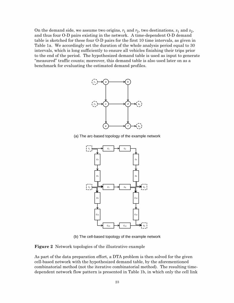
On the demand side, we assume two origins, and , two destinations, and ,

and thus four O-D pairs existing in the network. A time-dependent O-D demand

table is sketched for these four O-D pairs for the first 10 time intervals, as given in

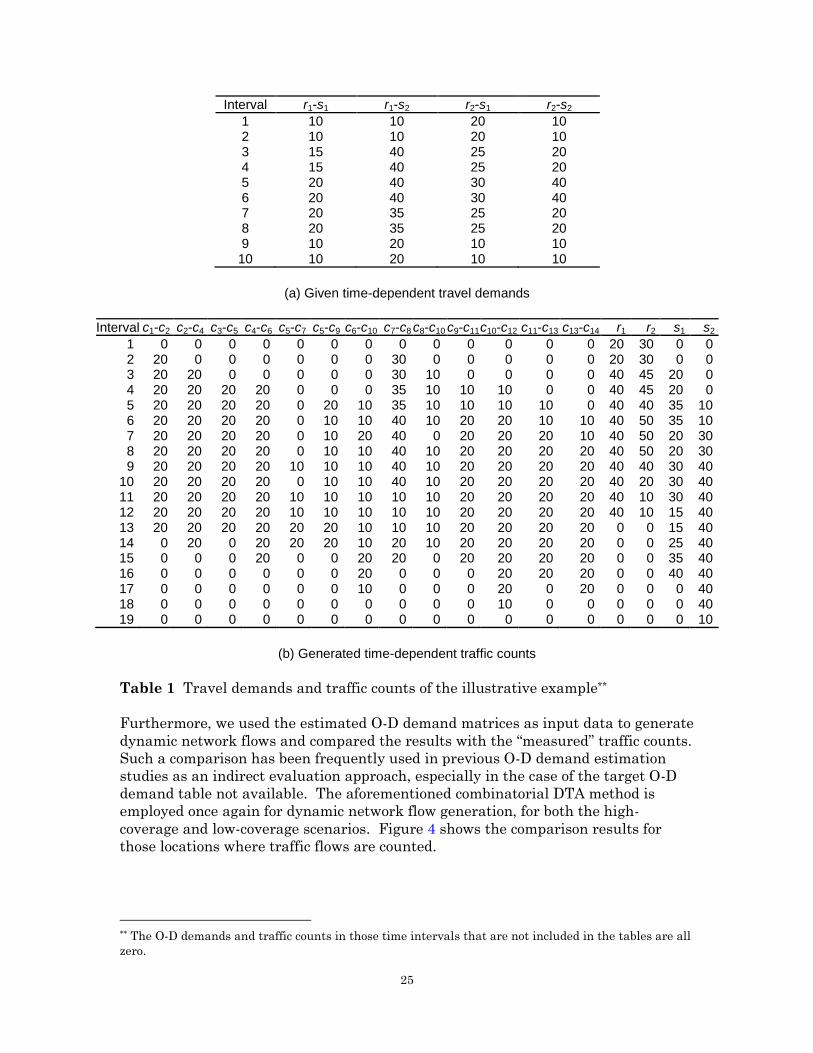
Table 1a. We accordingly set the duration of the whole analysis period equal to 30

intervals, which is long sufficiently to ensure all vehicles finishing their trips prior

to the end of the period. The hypothesized demand table is used as input to generate

“measured” traffic counts; moreover, this demand table is also used later on as a

benchmark for evaluating the estimated demand profiles.

(a) The arc-based topology of the example network

(b) The cell-based topology of the example network

Figure 2 Network topologies of the illustrative example

As part of the data preparation effort, a DTA problem is then solved for the given

cell-based network with the hypothesized demand table, by the aforementioned

combinatorial method (not the iterative combinatorial method). The resulting time-

dependent network flow pattern is presented in Table 1b, in which only the cell link

a

c

b

d

e f

r1

r2 s1

s2

c1 c2

c3

c5

c7 c8

c4

c6

c9

c11

c10

c12

c13 c14

r1

r2 s1

s2

24

flows, outgoing origin flows, and incoming destination flows are listed. The flows

through some cell links and origin/destination cordons are aggregated and saved as

“measured” link or cordon counts for the O-D demand estimation problem. For the

sake of comparison, we assume two data availability scenarios: 1) a high-coverage

scenario; 2) a low-coverage scenario. In the first scenario, traffic counts are

measured at origins and and on cell links - , - , - , - and - .

Note that the cordon count at any origin is the sum of relevant link flows, i.e.,

and . In the second scenario, we

assume that traffic counts are measured only on cell links - , - , - and -

. We also assume that traffic counts are accurately measured for all time

intervals without any measurement noise.

In addition to the supply and demand data given above, a set of modeling

parameters need to be specified for the proposed solution procedure. Two sets of

parameters 0.1 and 0.05 are assumed*. These parameters are

weighting coefficients used to convert path deviation costs to path travel times and

to convert path entropy costs to path travel times, respectively.

The experiment of applying the iterative solution procedure for the two scenarios

was conducted with the convergence gap 0.001 and the maximum iteration

number 50. In the application, the iterative procedure stops when either of the

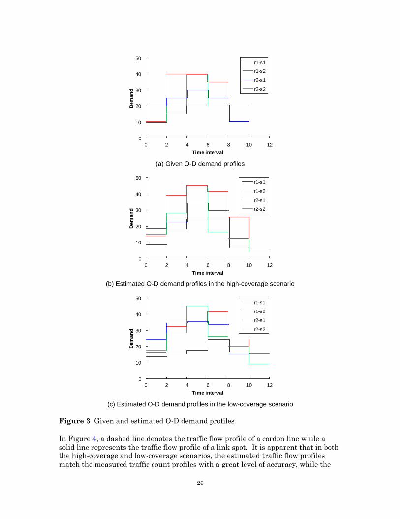
convergence criteria is satisfied. The obtained demand estimation results of all O-D

pairs from the two scenarios are depicted in Figure 3 and are evaluated by

comparing them with the given O-D demand profiles from Table 1.

Note here that the O-D demands are estimated in terms of the demand estimation

interval (rather than the demand departure interval ). For this example

problem, we set , as mentioned previously, so the demand profiles in

Figure 3 show a time-varying pattern with a step of two time intervals. The

estimation performance is assessed by simply comparing the given and estimated O-

D demand profiles. First, we observed that the two estimated O-D demand profiles

capture the temporal pattern of the given profiles on a certain level of accuracy,

though the estimation accuracy seems to vary quite largely across O-D pairs. In

particular, the demand profile of O-D pair - is estimated relatively better than

other O-D pairs in both the scenarios. The possible reason is due to the simple

structure of this O-D pair, in that it has only one path. Second, we noted that the

demand estimation result in the high-coverage scenario is apparently better than

that in the low-coverage scenario. This observation is consistent with our common

sense that higher network coverage of traffic measurements provides more

information about the network flows and hence produces a better estimation result if

these measurements are not biased. As an aggregated comparison, we calculated

the root mean square error (RMSE) of the estimated O-D demands against the given

O-D demands for both the scenarios. The calculation result shows that the RMSE of

the high-coverage scenario is 4.29 veh per interval while the RMSE of the low-

coverage scenario is 6.25 veh per interval.

* It should be noted that these parameter values are arbitrarily specified for this small example.

25

Interval r1-s1 r1-s2 r2-s1 r2-s2

1 10 10 20 10 2 10 10 20 10 3 15 40 25 20 4 15 40 25 20 5 20 40 30 40 6 20 40 30 40 7 20 35 25 20 8 20 35 25 20 9 10 20 10 10 10 10 20 10 10

(a) Given time-dependent travel demands

Interval c1-c2 c2-c4 c3-c5 c4-c6 c5-c7 c5-c9 c6-c10 c7-c8 c8-c10 c9-c11 c10-c12 c11-c13 c13-c14 r1 r2 s1 s2

1 0 0 0 0 0 0 0 0 0 0 0 0 0 20 30 0 0 2 20 0 0 0 0 0 0 30 0 0 0 0 0 20 30 0 0 3 20 20 0 0 0 0 0 30 10 0 0 0 0 40 45 20 0 4 20 20 20 20 0 0 0 35 10 10 10 0 0 40 45 20 0 5 20 20 20 20 0 20 10 35 10 10 10 10 0 40 40 35 10 6 20 20 20 20 0 10 10 40 10 20 20 10 10 40 50 35 10 7 20 20 20 20 0 10 20 40 0 20 20 20 10 40 50 20 30 8 20 20 20 20 0 10 10 40 10 20 20 20 20 40 50 20 30 9 20 20 20 20 10 10 10 40 10 20 20 20 20 40 40 30 40

10 20 20 20 20 0 10 10 40 10 20 20 20 20 40 20 30 40 11 20 20 20 20 10 10 10 10 10 20 20 20 20 40 10 30 40 12 20 20 20 20 10 10 10 10 10 20 20 20 20 40 10 15 40 13 20 20 20 20 20 20 10 10 10 20 20 20 20 0 0 15 40 14 0 20 0 20 20 20 10 20 10 20 20 20 20 0 0 25 40 15 0 0 0 20 0 0 20 20 0 20 20 20 20 0 0 35 40 16 0 0 0 0 0 0 20 0 0 0 20 20 20 0 0 40 40 17 0 0 0 0 0 0 10 0 0 0 20 0 20 0 0 0 40 18 0 0 0 0 0 0 0 0 0 0 10 0 0 0 0 0 40 19 0 0 0 0 0 0 0 0 0 0 0 0 0 0 0 0 10

(b) Generated time-dependent traffic counts

Table 1 Travel demands and traffic counts of the illustrative example**

Furthermore, we used the estimated O-D demand matrices as input data to generate

dynamic network flows and compared the results with the “measured” traffic counts.

Such a comparison has been frequently used in previous O-D demand estimation

studies as an indirect evaluation approach, especially in the case of the target O-D

demand table not available. The aforementioned combinatorial DTA method is

employed once again for dynamic network flow generation, for both the high-

coverage and low-coverage scenarios. Figure 4 shows the comparison results for

those locations where traffic flows are counted.

** The O-D demands and traffic counts in those time intervals that are not included in the tables are all

zero.

26

(a) Given O-D demand profiles

(b) Estimated O-D demand profiles in the high-coverage scenario

(c) Estimated O-D demand profiles in the low-coverage scenario

Figure 3 Given and estimated O-D demand profiles

In Figure 4, a dashed line denotes the traffic flow profile of a cordon line while a

solid line represents the traffic flow profile of a link spot. It is apparent that in both

the high-coverage and low-coverage scenarios, the estimated traffic flow profiles

match the measured traffic count profiles with a great level of accuracy, while the

0

10

20

30

40

50

0 2 4 6 8 10 12

Dem

an

d

Time interval

r1-s1

r1-s2

r2-s1

r2-s2

0

10

20

30

40

50

0 2 4 6 8 10 12

Dem

an

d

Time interval

r1-s1

r1-s2

r2-s1

r2-s2

0

10

20

30

40

50

0 2 4 6 8 10 12

Dem

an

d

Time interval

r1-s1

r1-s2

r2-s1

r2-s2

27

average match error in the high-coverage scenario appears considerably lower. In

particular, the RMSE values of the estimated traffic flows against the measured

traffic counts in the two scenarios are 3.69 and 4.22 veh per interval, respectively.

This result is consistent with the above O-D demand comparison result.

(a) Measured cordon and link flow profiles

(b) Estimated cordon and link flow profiles in the high-coverage scenario

(c) Estimated link flow profiles in the low-coverage scenario

Figure 4 Measured and estimated cordon and link flow profiles

0

10

20

30

40

50

0 5 10 15 20 25 30

Tra

ffic

flo

w

Time interval

c1-c2

c3-c5

c10-c12

c13-c14

0

10

20

30

40

50

0 5 10 15 20 25 30

Tra

ffic

co

un

t

Time interval

r1

r2

c1-c2

c3-c5

c7-c8

c10-c12

c13-c14

0

10

20

30

40

50

0 5 10 15 20 25 30

Tra

ffic

flo

w

Time interval

r1

r2

c1-c2

c3-c5

c7-c8

c10-c12

c13-c14

28

The above numerical results merely summarize our initial observation on the

performance of the proposed excess-demand DTA approach for estimating O-D

demand matrices. The developed modeling and solution framework should be

further applied to problems of larger size and with a variety of different network

settings in terms of network topology, road capacity, demand level, and so on. Given

that the solution procedure is a de facto process of repeatedly solving an excess-

demand DTA problem, we are also interested in building the framework based on an

existing DTA solver (e.g., Visual Interactive System for Transportation Applications

(VISTA)†) that can solve large-scale network problems in a reasonable timeframe.

In addition, other tests are worth being conducted to examine the effect or

sensitivity of various modeling parameters or components, such as the demand

estimation interval length, the traffic measurement interval length, the weighting

coefficients, and the traffic flow model used in the DTA process. Till these tests are

sufficiently conducted, we will then be able to have a more thorough understanding

about the estimator’s behavioral and accuracy performance and may gain additional

insights about how to further improve its performance.

6. Concluding remarks

This paper presents a new composite equilibrium approach for the dynamic O-D

demand matrix estimation problem, in which its underlying equilibrium conditions

are a synthetic result of minimization of individual routing costs, minimization of

traffic count matching errors, and maximization of O-D demand entropies. The

composite equilibrium conditions are characterized by a VI model, and in

accordance, the solution existence, equivalence and uniqueness of the O-D demand

estimation problem are proved by the VI techniques. To relax the solution

complexity, the O-D demand estimation problem is reformulated as an excess-

demand DTA problem defined for an expanded network with dummy paths, by

supplying an upper bound of travel demand and a dummy path cost for each O-D

pair and each time interval. The excess-demand formulation enables us to apply

existing DTA solution methods for inferring the path flow pattern in the expanded

network and thus estimating O-D demand matrices for the original network. We

sketched an iterative solution procedure, which resorts to repeatedly solving the

excess-demand DTA problem and adjusting the dummy path costs. The

computational bottleneck of this procedure lies in solving the excess-demand DTA

problem. In our implementation, an iterative combinatorial algorithm is suggested

for the DTA solutions.

It should be emphasized that the proposed modeling and solution framework is quite

general in the sense of its applicability and modularity, in which the traffic

dynamics can be modeled by other network flow models than the CTM theory. In

our case, as we have seen, two optimization criteria, namely, minimization of

squared traffic count errors and maximization of O-D demand entropies, are

incorporated into the composite equilibrium conditions. When needed, other

analytical or statistical optimization principles could be introduced into the model in

† The Network Modeling Center at University of Texas at Austin uses VISTA as a routine DTA

software package for many dynamic network analysis and demand forecasting applications.

29

a similar way. On the solution side, alternative analytical or simulation-based DTA

solution methods and dummy path cost adjustment procedures can be potentially

inserted into the iterative solution procedure. A set of experiments of implementing

and comparing different solution algorithms for these two tasks should be further

conducted to identify the most effective and efficient solution procedure.

Acknowledgements

This research is funded by Texas Department of Transportation (TxDOT) and

Capital Area Metropolitan Planning Organization (CAMPO) through the Network

Modeling Center at University of Texas at Austin. The first author is also supported

by a research grant along with his Young Talent Award from the China Recruitment

Program of Global Experts and a research grant from the State Key Laboratory of

Ocean Engineering at Shanghai Jiao Tong University (Grant No.: GKZD010061).

The authors are grateful to the Editor-in-Chief, Professor Terry Friesz, and two

anonymous referees for their constructive suggestions. However, the authors claim

that they are solely responsible for the facts and the accuracy of the data presented

herein.

References

Anas, A. 1983. Discrete choice theory, information theory, and the multinomial logit

and gravity models. Transportation Research Part B, 17(1), 13-23.

Bell, M.G.H., Shield, C.M., Busch, F. and Kruse, G. 1997. A stochastic user

equilibrium path flow estimator. Transportation Research Part B, 5(3/4), 197-210.

Cascetta, E., Inaudi, D. and Marquis, G. 1993. Dynamic estimators of origin-

destination matrices using traffic counts. Transportation Science, 27(4), 363-373.

Chiu, Y.C. and Zheng, H. 2007. Real-time mobilization decisions for multi-priority

emergency response resources and evacuation groups: Model formulation and

solution. Transportation Research Part E, 43(6), 710-736.

Choi, K., Jayakrishan, R., Kim, H., Yang, I. and Lee, J. 2009. Dynamic origin-

destination estimation using dynamic traffic simulation model in an urban arterial

corridor. Transportation Research Record, 2133, 133-141.

Chung, B.D., Yao, T., Xie, C. and Thorsen, A. 2011. Robust optimization model for a

dynamic network design problem under demand uncertainty. Networks and Spatial

Economics, 11(2), 371-389.

Cipriani, E., Florian, M., Mahut, M. and Nigro, M. 2011. A gradient approximation

approach for adjusting temporal origin-destination matrices. Transportation

Research Part C, 19(2), 270-282.

30

Daganzo, C.F. 1994. The cell transmission model: A simple dynamic representation

of highway traffic consistent with the hydrodynamic theory. Transportation

Research Part B, 28(4), 269-287.

Daganzo, C.F. 1995. The cell transmission model, part II: Network traffic.

Transportation Research Part B, 29(2), 79-93.

Facchinei, F. and Pang, J.S. 2003. Finite-Dimensional Variational Inequalities and

Complementarity Problems: Volume I. Springer-Verlag, New York, NY.

Friesz, T.L., Bernstein, D., Smith, T.E., Tobin, R.L. and Wei, B.W. 1993. A

variational inequality formulation of the dynamic network equilibrium problem.

Operations Research, 41(1), 179–191.

Golani, H. and Waller, S.T. 2004. Combinatorial approach for multiple-destination

user optimal dynamic traffic assignment. Transportation Research Record, 1882, 70-

78.

Karoonsoontawong, A. and Waller, S.T. 2010. Integrated network capacity

expansion and traffic signal optimization problem: Robust bi-level dynamic

formulation. Networks and Spatial Economics, 10(4), 525-550.

Kattan, L. and Abdulhai, B. 2006. Noniterative approach to dynamic traffic origin-

destination estimation with parallel evolutionary algorithms. Transportation

Research Record, 1964, 201-210.

LeBlanc, L.J. and Farhangian, K. 1982. Selection of a trip table which reproduces

observed link flows. Transportation Research Part B, 16(2), 83-88.

Lighthill, M.J. and Whitham, G.B. 1955. On kinematic waves II: A theory of traffic

flow on long crowded roads. Proceedings of the Royal Society of London, Series A:

Mathematical and Physical Sciences, 229(1178), 317-345.

Lo, H.K. 2001. A cell-based traffic control formulation: Strategies and benefits of

dynamic timing plans. Transportation Science, 35(2), 148-164.

Lo, H.K. and Szeto, W.Y. 2002. A cell-based variational inequality formulation of the

dynamic user optimal assignment problem. Transportation Research Part B, 36(5),

421-433.

Mahut, M., Florian, M., Tremblay, N., Campbell, M., Patman, D. and McDaniel, Z.K.

2004. Calibration and application of a simulation-based dynamic traffic assignment

model. Transportation Research Record, 1876, 101-111.

Nie, Y. 2006. A Variational Inequality Approach for Inferring Dynamic Origin-

Destination Travel Demands. Ph.D. Thesis, Department of Civil and Environmental

Engineering, University of California, Davis, CA.

31

Nie, Y. and Zhang, H.M. 2008. A variational inequality formulation for inferring

dynamic origin-destination travel demands. Transportation Research Part B, 42(7-

8), 635-662.

Nie, Y. and Zhang, H.M. 2010. A relaxation approach for estimating origin–

destination trip tables. Networks and Spatial Economics, 10(1), 147-172.

Nguyen, S. 1977. Estimating an O-D Matrix from Network Data: A Network

Equilibrium Approach. Publication No. 87, Centre de Recherche sur les Transports,

Université de Montréal, Montreal, QC.

Richards, P.I. 1956. Shock waves on the highway. Operations Research, 34(1), 42-51.

Sheffi, Y. 1985. Urban Transportation Networks: Equilibrium Analysis with

Mathematical Programming Methods. Prentice-Hall, Englewood Cliffs, NJ.

Shen, W. and Wynter, L. 2011. A New One-Level Convex Optimization Approach for

Estimating Origin-Destination Demand. IBM Research Report RC25147, Thomas J.

Watson Research Center, Yorktown Heights, NY.

Smith, M.J. 1993. A new dynamic traffic model and the existence and calculation of

dynamic user equilibria on congested capacity-constrained road networks.

Transportation Research Part B, 26(1), 49–63.

Spiess, H. 1990. A Gradient Approach for the O-D Matrix Adjustment Problem.

Publication No. 693, Centre de Recherche sur les Transports, Université de

Montréal, Montreal, QC.

Tavana, H. 2001. Internally Consistent Estimation of Dynamic Network Origin-

Destination Flows from Intelligent Transportation Systems Data Using Bi-Level

Optimization. Ph.D. Thesis, Department of Civil Engineering, University of Texas,

Austin, TX.

Turnquist, M.A. and Gur, Y. 1979. Estimation of trip tables from observed link

volumes. Transportation Research Record, 730, 1-6.

Ukkusuri, S. and Waller, S.T. 2008. Linear programming models for the user and

system optimal dynamic network design problem: Formulations, comparisons and

extensions. Networks and Spatial Economics, 8(4), 383-406.

Van Zuylen, H.J. and Willumsen, L.G. 1980. The most likely trip matrix estimated

from traffic counts. Transportation Research Part B, 14(3), 281-293.

Waller, S.T., Mouskos, K.C., Kamaryiannis, D. and Ziliaskopoulos, A.K. 2006. A

linear model for the continuous network design problem. Computer-Aided Civil and

Infrastructure Engineering, 21(5), 334-345.

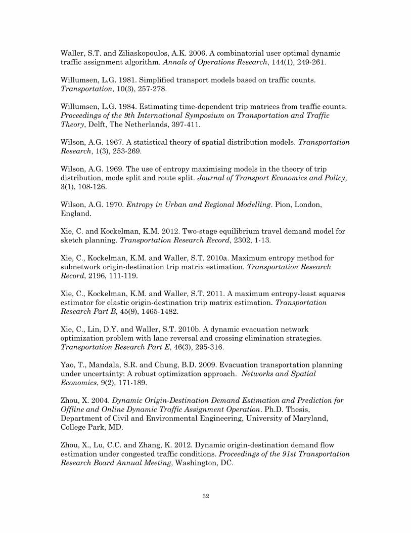
32

Waller, S.T. and Ziliaskopoulos, A.K. 2006. A combinatorial user optimal dynamic

traffic assignment algorithm. Annals of Operations Research, 144(1), 249-261.

Willumsen, L.G. 1981. Simplified transport models based on traffic counts.

Transportation, 10(3), 257-278.

Willumsen, L.G. 1984. Estimating time-dependent trip matrices from traffic counts.

Proceedings of the 9th International Symposium on Transportation and Traffic

Theory, Delft, The Netherlands, 397-411.

Wilson, A.G. 1967. A statistical theory of spatial distribution models. Transportation

Research, 1(3), 253-269.

Wilson, A.G. 1969. The use of entropy maximising models in the theory of trip

distribution, mode split and route split. Journal of Transport Economics and Policy,

3(1), 108-126.

Wilson, A.G. 1970. Entropy in Urban and Regional Modelling. Pion, London,

England.

Xie, C. and Kockelman, K.M. 2012. Two-stage equilibrium travel demand model for

sketch planning. Transportation Research Record, 2302, 1-13.

Xie, C., Kockelman, K.M. and Waller, S.T. 2010a. Maximum entropy method for

subnetwork origin-destination trip matrix estimation. Transportation Research

Record, 2196, 111-119.

Xie, C., Kockelman, K.M. and Waller, S.T. 2011. A maximum entropy-least squares

estimator for elastic origin-destination trip matrix estimation. Transportation

Research Part B, 45(9), 1465-1482.

Xie, C., Lin, D.Y. and Waller, S.T. 2010b. A dynamic evacuation network

optimization problem with lane reversal and crossing elimination strategies.

Transportation Research Part E, 46(3), 295-316.

Yao, T., Mandala, S.R. and Chung, B.D. 2009. Evacuation transportation planning

under uncertainty: A robust optimization approach. Networks and Spatial

Economics, 9(2), 171-189.

Zhou, X. 2004. Dynamic Origin-Destination Demand Estimation and Prediction for

Offline and Online Dynamic Traffic Assignment Operation. Ph.D. Thesis,

Department of Civil and Environmental Engineering, University of Maryland,

College Park, MD.

Zhou, X., Lu, C.C. and Zhang, K. 2012. Dynamic origin-destination demand flow

estimation under congested traffic conditions. Proceedings of the 91st Transportation

Research Board Annual Meeting, Washington, DC.

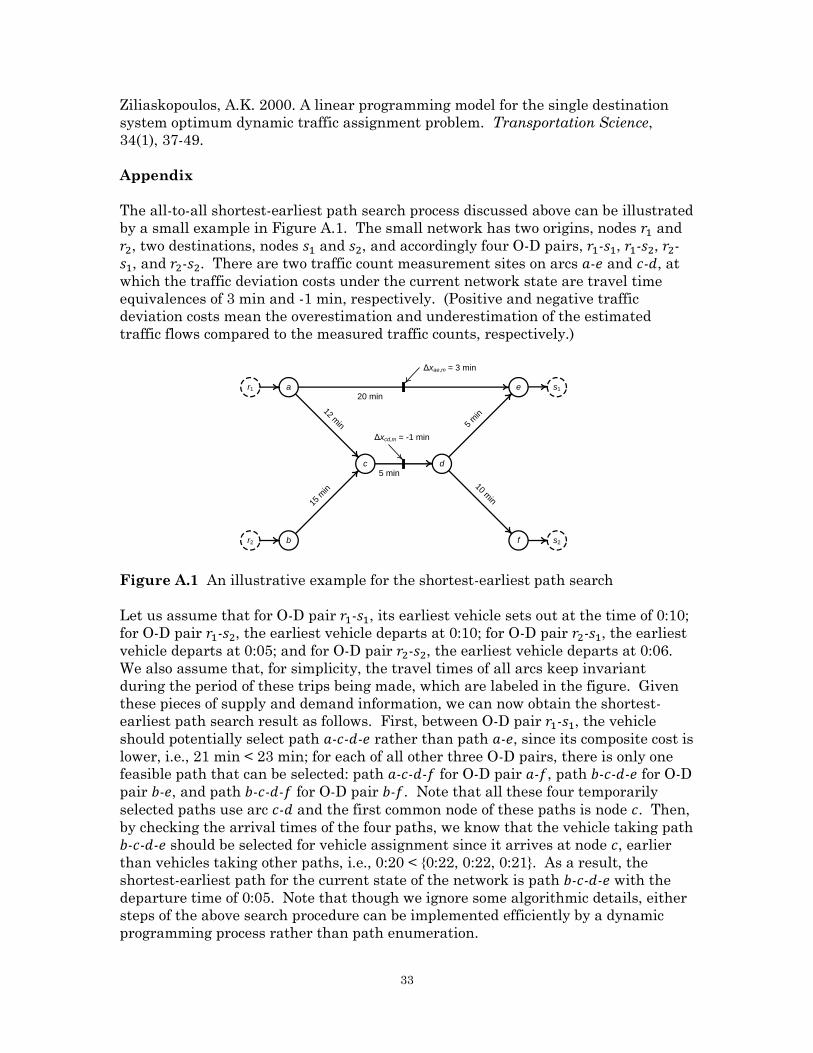
33

Ziliaskopoulos, A.K. 2000. A linear programming model for the single destination

system optimum dynamic traffic assignment problem. Transportation Science,

34(1), 37-49.

Appendix

The all-to-all shortest-earliest path search process discussed above can be illustrated

by a small example in Figure A.1. The small network has two origins, nodes and

, two destinations, nodes and , and accordingly four O-D pairs, - , - , -

, and - . There are two traffic count measurement sites on arcs - and - , at

which the traffic deviation costs under the current network state are travel time

equivalences of 3 min and -1 min, respectively. (Positive and negative traffic

deviation costs mean the overestimation and underestimation of the estimated

traffic flows compared to the measured traffic counts, respectively.)

Figure A.1 An illustrative example for the shortest-earliest path search

Let us assume that for O-D pair - , its earliest vehicle sets out at the time of 0:10;

for O-D pair - , the earliest vehicle departs at 0:10; for O-D pair - , the earliest

vehicle departs at 0:05; and for O-D pair - , the earliest vehicle departs at 0:06.

We also assume that, for simplicity, the travel times of all arcs keep invariant

during the period of these trips being made, which are labeled in the figure. Given

these pieces of supply and demand information, we can now obtain the shortest-

earliest path search result as follows. First, between O-D pair - , the vehicle

should potentially select path - - - rather than path - , since its composite cost is

lower, i.e., 21 min < 23 min; for each of all other three O-D pairs, there is only one

feasible path that can be selected: path - - - for O-D pair - , path - - - for O-D

pair - , and path - - - for O-D pair - . Note that all these four temporarily

selected paths use arc - and the first common node of these paths is node . Then,

by checking the arrival times of the four paths, we know that the vehicle taking path

- - - should be selected for vehicle assignment since it arrives at node , earlier

than vehicles taking other paths, i.e., 0:20 < {0:22, 0:22, 0:21}. As a result, the

shortest-earliest path for the current state of the network is path - - - with the

departure time of 0:05. Note that though we ignore some algorithmic details, either

steps of the above search procedure can be implemented efficiently by a dynamic

programming process rather than path enumeration.

a

c

e

d

b f

r1

r2

s1

s2

Δxae,m = 3 min

20 min

5 min

12 min

15 m

in

5 m

in

10 min

Δxcd,m = -1 min