AlgorithmicaDOI 10.1007/s00453-007-9055-0

Inferring (Biological) Signal Transduction Networksvia Transitive Reductions of Directed Graphs

Réka Albert · Bhaskar DasGupta ·Riccardo Dondi · Eduardo Sontag

Received: 8 December 2005 / Accepted: 27 November 2006© Springer Science+Business Media, LLC 2007

Abstract In this paper we consider the p-ary transitive reduction (TRp) problemwhere p > 0 is an integer; for p = 2 this problem arises in inferring a sparsest pos-sible (biological) signal transduction network consistent with a set of experimentalobservations with a goal to minimize false positive inferences even if risking falsenegatives. Special cases of TRp have been investigated before in different contexts;the best previous results are as follows:

(1) The minimum equivalent digraph problem, that correspond to a special case ofTR1 with no critical edges, is known to be MAX-SNP-hard, admits a polynomialtime algorithm with an approximation ratio of 1.617 + ε for any constant ε > 0

R. Albert’s research was partly supported by a Sloan Research Fellowship in Science andTechnology.B. DasGupta’s research was partly supported by NSF grants DBI-0543365, IIS-0612044 andIIS-0346973.E. Sontag’s research was partly supported by NSF grants EIA 0205116 and DMS-0504557.

R. AlbertDepartment of Physics, Pennsylvania State University, University Park, PA 16802, USAe-mail: ralbert@phys.psu.edu

B. DasGupta (�)Department of Computer Science, University of Illinois at Chicago, Chicago, IL 60607, USAe-mail: dasgupta@cs.uic.edu

R. DondiDipartimento di Scienze dei Linguaggi, della Comunicazione e degli Studi Culturali,Università degli Studi di Bergamo, Bergamo 24129, Italye-mail: riccardo.dondi@unimib.it

E. SontagDepartment of Mathematics, Rutgers University, New Brunswick, NJ 08903, USAe-mail: sontag@math.rutgers.edu

Algorithmica

(Chiu and Liu in Sci. Sin. 4:1396–1400, 1965) and can be solved in linear timefor directed acyclic graphs (Aho et al. in SIAM J. Comput. 1(2):131–137, 1972).

(2) A 2-approximation algorithm exists for TR1 (Frederickson and JàJà in SIAM J.Comput. 10(2):270–283, 1981; Khuller et al. in 19th Annual ACM-SIAM Sym-posium on Discrete Algorithms, pp. 937–938, 1999).

In this paper, our contributions are as follows:

• We observe that TRp, for any integer p > 0, can be solved in linear time for di-rected acyclic graphs using the ideas in Aho et al. (SIAM J. Comput. 1(2):131–137,1972).

• We provide a 1.78-approximation for TR1 that improves the 2-approximation men-tioned in (2) above.

• We provide a 2 + o(1)-approximation for TRp on general graphs for any fixedprime p > 1.

Keywords Transitive reduction of directed graphs · Minimum equivalent digraph ·(Biological) signal transduction networks · Approximation algorithms

1 Introduction

In this paper, we study the p-ary transitive reduction problem which can be definedas follows. We are given a directed graph G = (V ,E) with an edge labeling functionw : E �→ {0,1,2, . . . , p − 1} for some fixed integer p > 0. The following definitionsand notations are used:

• All paths are (possibly self-intersecting) directed paths unless otherwise stated. Anon-self-intersecting path or cycle is called a simple path or cycle.

• If edge labels are removed or not mentioned, they are be assumed to be 0 for thepurpose of any problem that needs them.

• The parity of a path P from vertex u to vertex v is∑

e∈P w(e) (modp). For thespecial case of p = 2, a path of parity 0 (resp., 1) is called a path of even (resp,odd) parity.

• The notation ux⇒ v denotes a path from u to v of parity x ∈ {0,1,2, . . . , p − 1}. If

we do not care about the parity, we simply denote the path as u ⇒ v. An edge willsimply be denoted by u

x→ v or u → v.• For a subset of edges E′ ⊆ E, reachable(E′) is the set of all ordered triples (u, v, x)

such that ux⇒ v is a path of the restricted subgraph (V ,E′).1

The p-ary transitive reduction problem is defined as follows:

Problem name: p-ary Transitive Reduction (TRp).Instance: A directed graph G = (V ,E) with an edge labeling function w : E �→{0,1,2, . . . , p − 1} and a set of critical edges Ecritical ⊆ E.

1We will sometimes simply say ux⇒ v is contained in E′ to mean u

x⇒ v is a path of the restricted subgraph(V ,E′).

Algorithmica

Valid Solutions: A subgraph G′ = (V ,E′) where Ecritical ⊆ E′ ⊆ E andreachable(E′) = reachable(E).

Objective: Minimize |E′|.We are specially interested in the special case of p = 2; the corresponding TR2

problem will be simply referred to as the Binary Transitive Reduction (BTR) prob-lem. In the next subsection, we explain the application of BTR to the problem ofinferring signal transduction networks in biology.

2 Motivations

Most biological characteristics of a cell arise from the complex interactions betweenits numerous constituents such as DNA, RNA, proteins and small molecules [2].Cells use signaling pathways and regulatory mechanisms to coordinate multiple func-tions, allowing them to respond to and acclimate to an ever-changing environment.Genome-wide experimental methods now identify interactions among thousands ofcellular components [10, 11, 17, 18]; however these experiments are rarely conductedin the specific cell type of interest, are not able to probe all possible interactions andregulatory mechanisms, and the resulting maps do not reflect the strength and tim-ing of the interactions. The existing theoretical literature on signaling is focused onnetworks where the elementary reactions and direct interactions are known [8, 12];however quantitative characterization of every reaction and regulatory interaction par-ticipating even in a relatively simple function of a single-celled organism requires aconcerted and decades-long effort. The state of the art understanding of many signal-ing processes is limited to the knowledge of key mediators and of their positive ornegative effects on the whole process.

Experimental information about the involvement of a specific component in agiven signal transduction network can be partitioned into three categories. First, bio-chemical evidence, that provides information on enzymatic activity or protein-proteininteractions. For example, in plant signal transduction, the putative G protein coupledreceptor GCR1 can physically interact with the G protein GPA1 as supported by split-ubiquitin and co-immunoprecipitation experiments [21]. Second, genetic evidence ofdifferential responses to a stimulus in wild-type organisms versus a mutant organismimplicates the product of the mutated gene in the signal transduction process. For ex-ample, the EMS-generated OST1 mutant is less sensitive to abscisic acid (ABA); thusone can infer that the OST1 protein is a part of the ABA signaling cascade [20]. Third,pharmacological evidence, in which a chemical is used either to mimic the elimina-tion of a particular component, or to exogenously provide a certain component, canlead to similar inferences. For example, a nitric oxide (NO) scavenger inhibits ABA-induced stomatal closure while a NO donor promotes stomatal closure, thus NO isa part of the ABA network [6]. The last two types of inference do not give directinteractions but correspond to pathways and pathway regulation. To synthesize allthis information into a consistent network, we need to determine how the differentpathways suggested by experiments fit together.

The BTR problem considered in this paper is useful for determining the sparsestgraph consistent with a set of experimental observations. Note that we are not as-suming that real signal transduction networks are the sparsest possible, since that is

Algorithmica

clearly not the case. Our goal is to minimize false positive (spurious) inferences, evenif risking false negatives.

The first requirement of our method is to distill experimental conclusions intoqualitative regulatory relations between cellular components. Following [5, 19, 22],we distinguish between positive and negative regulation, usually denoted by theverbs “promote” and “inhibit” and represented graphically as → and �. Biochemicalevidence is represented as component-to-component relationships, such as “A pro-motes B”. However, both genetic and pharmacological evidence leads to inferencesof the type “C promotes process(A promotes B)”. In this case we use one of the fol-lowing three representations (i) if the process describes an enzymatic reaction, werepresent it as both A and C activating B; (ii) if the interaction between A and B isdirect and C does not have a catalytic role, we assume that C activates A; (iii) in allother cases we assume that C activates an unknown intermediary vertex of the ABpathway.

Most edges of the obtained directed graph will not correspond to direct interac-tions, but starting and end points of directed paths in the (unknown) interaction graph,in other words they represent reachability relationships. Thus our goal is to find thesparsest graph that maintains all reachability relationships, or the minimal transitivereduction of the starting graph. Arcs of the starting graph corresponding to directinteractions will be marked as such and will need to be maintained during the transi-tive reduction algorithm. A path between node i and j is inhibitory if it contains anodd number of inhibitory interactions. Thus indirect inhibitory edges will need to bereduced to paths that contain an odd number of inhibitory edges. It is this transitivereduction problem that is formalized as the BTR problem where edge labels 0 and1 correspond to activations and inhibitions, respectively, and a set of critical edgesEcritical ⊆ E corresponding to direct interactions.

For the sake of completeness, we briefly describe the entire approach of mini-mizing the network (see [19] for a specific example done by manual curation). Westart by synthesizing the vertex-to-vertex reachability relationships, then we turn tothe vertex-to-path influences. If existing paths already explains a vertex-to-path rela-tionship, no new intermediaries need to be added, otherwise we incorporate it in oneof the three representations described above. Next we determine the obtained graph’stransitive reduction subject to the constraints that no edges flagged as direct are elimi-nated. Finally we identify and collapse pairs of equivalent intermediary vertices (e.g.,adjacent vertices in a linear chain) if that procedure does not change the reachabilityrelationships of the real vertices.

Figure 1 shown here illustrates the graph synthesis process in two cases (specifiedby the reachability sets and pathway influence information displayed on the left side)that differ in a single reachability relationship only. In both cases the edges markedas dashed on the top graph will be eliminated. In the first case the pathway regula-tory information is already incorporated thus no new intermediary vertices need to beadded. In the second case the relationship between C, A and E necessitates the addi-tion of a new vertex x. The addition of the BE edge would make B and x equivalentin terms of reachability; thus x could be identified with B.

Algorithmica

Fig. 1 Illustration of the graphsynthesis process in two cases

3 Previous Results

A given strongly connected directed graph G = (V ,E) on n vertices has a Hamil-tonian cycle if and only if an instance of the TR1 problem with G as input andEcritical = ∅ has an optimal solution with exactly n edges. Thus TRp is NP-completesince TR1 includes the problem of finding directed Hamiltonian cycle in a graph. TheTR1 problem with Ecritical = ∅ was called the minimum equivalent digraph (MED)problem by previous researchers. MED is known to be MAX-SNP-hard, admits apolynomial time algorithm with an approximation ratio of 1.617 + ε for any constantε > 0 [13] and can be solved in polynomial time for directed acyclic graphs [1].

A weighted version of the MED problem, in which each edge has a non-negativereal weight and the goal is to find a solution with a least value of the sum of weightsof the edges in the solution, admits a 2-approximation [9, 15]. This implies a 2-approximation for TR1 without the restriction Ecritical = ∅ in the following man-ner: given an instance of TR1, set the weight of every edge in Ecritical to zero, setthe weights of all other edges to 1 and run the 2-approximation algorithm for theweighted version of the MED problem.

4 Summary of Our Results

In this paper we investigate the TRp problem with a special emphasis on p > 1 sinceTR2 captures the most important part of the network minimization algorithm men-tioned in the introduction, namely that of finding efficient approximate solution ofthe binary transitive reduction (BTR) problem. The rest of the paper is organized asfollows:

• In Sect. 6, we observe that TRp for any p > 0 can be solved in polynomial time fordirected acyclic graphs using the ideas in [1]. The solution is valid even if a moregeneral version of the problem is considered.

• In Sect. 7.3 we provide a 1.78-approximation for TR1 and a 2 + o(1)-approxima-tion for TRp for any fixed prime p > 1 when the given graph is strongly connected.

Algorithmica

• In Sect. 7.4 we generalize the approximation results of the previous section toprovide a 1.78-approximation for TR1 and a 2 + o(1)-approximation for TRp forany fixed prime p > 1 for any given graph; the 1.78-approximation for TR1 forarbitrary graphs improves the previous 2-approximation for this case [9, 15].

Informally, our approach for solving TRp for general graphs involve developing ap-proximate solutions for strongly connected components and then combining thesesolutions. Because of the presence of edge labels which participate via a modulo p

addition in the parity of a path and the existence of critical edges, our solution differsfrom that in [9, 13, 15]. We combine these solutions via appropriate modifications toour solutions for TRp on DAG and via designs of “gadgets” that would ensure thatparities of various paths are preserved.

5 Basic Notations and Terminologies

An approximation algorithm for a minimization problem, that seeks to minimizean objective function, of performance or approximation ratio α (or simply an α-approximation) is a polynomial-time algorithm that provides a solution with a valueof the objective function that is at most α times the optimal value of the objectivefunction. We also use the following notations for convenience:

• OPT(G) = |Eopt(G)| denotes the number of edges in an optimal solution Eopt(G)

of TRp for the graph G.• ⊕p,�p and =p denote addition, subtraction and equality modulo p.

The following fact from elementary number theory will prove very useful to us.

Fact 1 For any prime p > 1 and any integer 0 < x < p, {i · x (modp)|0 < i < p + 1} = {0,1, . . . , p − 1}.

6 Polynomial-time Solution for Directed Acyclic Graphs (DAG)

Here we show that the TRp problem and in fact a more general version of it, whichwe refer to as the “grouped TRp problem with c-limited overlap”, can be solved inpolynomial time if the input graph is a DAG and c is a constant. We formally definethis general version of the problem below.

Definition 1 A grouped TRp problem with c-limited overlap on a graph G is definedas follows.

• The input graph G = (V ,E) is an instance of the TRp problem.• Non-empty distinct groups E1,E2, . . . ,Et of E are given such that:

–⋃t

i=1 Ei = E;– Ei �= Ej if i �= j ;– Ei �= ∅ for i ∈ {1,2, . . . , t};– The groups have overlaps “limited” by c, i.e., there is a partition I1, I2, . . . , Iq

of the set of indices {1,2, . . . , t} such that

Algorithmica

∗ Any two groups with indices from different sets of the partition do not inter-sect, i.e., for all i, j, x, y with i �= j and x ∈ Ii, y ∈ Ij , Ex ∩ Ey = ∅.

∗ The total number of edges in the groups with indices in any one set of thepartition is at most c, i.e., for all i, | ∪x∈Ii

Ex | ≤ c.• For each i ∈ {1,2, . . . , t}, a valid solution must contain all the edges in Ei or none

of the edges in Ei .• We are also given a set of critical edges Ecritical ⊆ E. Any solution must contain

every edge in Ecritical.

Example 1 (Illustration of the grouped TRp problem with 6-limited overlap) Sup-pose that G = (V ,E) is an instance of the grouped TRp problem with E ={e1, e2, e3, . . . , e9}, t = 4, E1 = {e1, e2, e4, e5, e9}, E2 = {e1, e2, e3}, E3 = {e6, e7},E4 = {e6, e7, e8}, q = 2, I1 = {1,2}, I2 = {3,4}. Then, this is an instance of a TRp

problem with 6-limited overlap on G since both |E1 ∪E2| and |E3 ∪E4| are no morethan 6 and no edge from E1 ∪ E2 belongs to E3 ∪ E4 (and vice versa). Moreover, bydefinition of grouped TRp problem with c-limited overlap, a valid solution for thisgrouped TRp problem on G is required to use:

• All or none of the edges in E1;• All or none of the edges in E2;• All or none of the edges in E3;• All or none of the edges in E4.

Note that the TRp problem is in fact an instance of the grouped TRp problem with1-limited overlap when each group of E contains exactly one edge and the partitionof the set of indices consists of singleton sets.

Lemma 2 The grouped TRp problem with c-limited overlap can be solved in poly-nomial time when the given graph G is a DAG and c is a constant.

Proof The algorithm shown below can be used; it essentially generalizes the ideasin [1]. The comments for various steps in the algorithm begin with //.

compute in O(|V | + |E|) time a topological sorting of G withv1, v2, . . . , vn as the topological order of nodes

start with the graph G′ = (V ,E′) with E′ = E and every edge in E′ marked as“not selected”for i = n − 1, n − 2, . . . ,1

for j = n,n − 1, n − 2, . . . , i + 1

for every edge viy→ vj ∈ E (in arbitrary order of y) // the edge is now

“examined”

if viy→ vj ∈ Ecritical then

mark viy→ vj as “selected”

else if there exists another path viy⇒ vj in G′

then E′ = E′ \ {viy→ vj } // the edge is redundant and thus deleted

from E′

Algorithmica

Fig. 2 Illustration of thealgorithm for the grouped TR3problem with 6-limited overlapon a DAG

else mark viy→ vj as “selected”

// Note that now E′ contains only edges marked as “selected”// first partition the edges in E′ based on their memberships in the partitionsindexed by I1, I2, . . . , Iq

let e1, e2, . . . , e|E′| be the edges in E′let J1, J2, . . . , Jr be a partition of the indices {1,2, . . . , |E′|} such that

for all � �= �′, both � and �′ belongs to the same set Js of the partitionif and only if both e� and e�′ are in

⋃x∈It

Ex for some t

// Notice that due to c-limitedness |⋃x:�∈Js∧e�∈ExEx | ≤ c for any set Js of the

partition;// thus, for any set Js of the partition, the numbers of edge groups Ex such that� ∈ Js and e� ∈ Ex is at most 2c;// thus, the following step takes constant time per Js by a trivial exhaustivemethod;// the most obvious exhaustive way takes O(22c

) = O(1) time per Js

E′′ = ∅for each s ∈ {1,2, . . . , r}

find a minimum collection of groups from {Ex : � ∈ Js ∧ e� ∈ Ex} thatincludes the edges in Js

add these edges to E′′output the final G′ = (V ,E′′) as the solution

For ease of understanding of the reader, we first work through a small exampleillustrating the above algorithm before continuing with the formal proof.

Example 2 (Illustration of the algorithm for the grouped TR3 problem with 6-limited overlap) Consider the DAG shown in Fig. 2 with p = 3, t = 3, E1 = {v5 →v6, v4 → v5, v3 → v4, v2 → v3, v2 → v5},E2 = {v5 → v6, v2 → v4},E3 = {v1 →v2},Ecritical = {v1 → v2}, q = 2, I1 = {1,2}, I2 = {3}. The instance is 6-limited sinceboth |E1 ∪ E2| and |E3| are no more than 6. The successive steps in the algorithmcan be summarized as follows:

• Mark all the edges as “not selected”;• Examine v5 → v6, mark the edge v5 → v6 as selected;• Examine v4 → v5, mark the edge v4 → v5, as selected;• Examine v3 → v4, mark the edge v3 → v4, as selected;

• Examine v2 → v5, remove this edge from E′ because of the path v20→ v4

2→ v5;

• Examine v2 → v4, remove this edge from E′ because of the path v21→ v3

2→ v4;• Examine v2 → v3, mark the edge v2 → v3, as selected;• Examine v1 → v2, mark the edge v1 → v2, as selected;

Algorithmica

• Now E′ = {e1 = v5 → v6, e2 = v4 → v5, e3 = v3 → v4, e4 = v2 → v3, e5 = v1 →v2}, and thus J1 = {1,2,3,4}, J2 = {5};

• A minimum collection of groups from E1 ∪ E2 that cover {e1, e2, e3, e4} is E1;• A minimum collection of groups from E3 that cover {e5} is E3;• The final solution E′′ = E1 ∪ E3.

The algorithm can be obviously implemented in polynomial time provided we can

check, for any given y, i and j , if there exists a path viy⇒ vj . This can be done

via a straightforward dynamic programming by using the following two well-knownobservations on topological sorting of any DAG:

(�) G does not contain a path vi ⇒ vj if i > j .(��) If G has a path vi ⇒ vj for some i ≤ j then any intermediate vertex vp of the

path satisfies i < p < j .

Moreover, no edge belonging to Ecritical is deleted and since an edge is deleted onlyif there is an alternate path of same parity between its two endpoints, reachable(E′) =reachable(E). Furthermore, either all the edges or none of the edges in any group ofedges are selected. Thus the algorithm returns a valid solution.

Now we continue with a formal proof of optimality of our algorithm. Notice thatan edge belongs to E′ if and only if it was marked as selected. To prove our algorithmis optimal, it suffices to show:

any valid solution must contain the edges in E′

since we have an exact algorithm to select a minimum number of groups to includethese edges. Note that the order in which pairs of vertices are examined by the nestedloops in the algorithm are:

(vn−1, vn)

then (vn−2, vn), (vn−2, vn−1)

then (vn−3, vn), (vn−3, vn−1), (vn−3, vn−2)

then (vn−4, vn), (vn−4, vn−1), (vn−4, vn−2), (vn−4, vn−3)...

and an edge viy→ vj is removed from E′ only when it is examined and an alternate

path viy⇒ vj exists in G. Thus, using Observations (�) and (��) the following holds:

(� � �) let viy→ vj be an edge in G such that an alternate path vi

y⇒ vj exists in G;

then when the edge viy→ vj is examined by the algorithm then some (not

necessarily the same as before) alternate path viy⇒ vj exists in G′.

Now we show that any valid solution must contain all the edges in E′. Suppose,for the sake of contradiction, that this is not the case and there is a valid solution thatdoes not contain at least one edge in E′. In the rest of the proof, we concentrate onthis valid solution. As we just said, there exists at least one edge that belongs to E′but does not belong to the valid solution. Among all such edges, let e be the first such

Algorithmica

edge examined during the execution of the algorithm. Now we have the followingsubcases:

Case 1.1. The reason why e = viy→ vj belongs to E′ is because of the following line

of code in our algorithm:

if viy→ vj ∈ Ecritical then

mark viy→ vj as “selected”

This implies that e ∈ Ecritical. But then e must belong to any valid solution, a con-tradiction.

Case 1.2. e �∈ Ecritical. The reason why e = viy→ vj belongs to E′ is because of the

last line of the following lines of code in our algorithm:

else if there exists another path viy⇒ vj in G′

then E′ = E′ \ {viy→ vj } // the edge is redundant and thus

deleted from E′

else mark viy→ vj as “selected”

The above last line of code was executed because there existed no other path viy⇒ vj

in G′ when the edge viy⇒ vj was examined. Via Observation (� � �) it follows that

there exists no other path viy⇒ vj in G either. Thus, any valid solution must contain

the edge e = viy→ vj , a contradiction. �

7 Efficient Approximation Algorithms for TRp

The goal of this section is to design an efficient approximation algorithm for TRp byproving the following result.

Theorem 3 There is a 2 + o(1)-approximation algorithm for TRp for any primep > 1 and a 1.78-approximation algorithm for TR1.

The next few subsections prove the above theorem step-by-step.

7.1 Characterization of Strongly Connected Components

Consider a strongly connected component C = (VC,EC) of the given graph G. Weconsider two types of such components:

Multiple Parity Components: for any two vertices u,v ∈ VC , ux⇒ v exists in C for

every x ∈ {0,1,2, . . . , p − 1}.Single Parity Components: for any two vertices u,v ∈ VC , u

x⇒ v exists in C forexactly one x from ∈ {0,1,2, . . . , p − 1}.

Algorithmica

Lemma 4 (a) Every strongly connected component of G is either of single parity orof multiple parity.

(b) A strongly connected component C is of multiple parity if and only if C con-tains a simple cycle of non-zero parity.

Proof Suppose that C is not a single parity component. Then there exists a pair of

vertices u and v such that uα⇒ v and u

β⇒ v exists in C with α �= β . Since C isstrongly connected, there exists a path, say of parity γ , from v to u. Since α �= β ,either α + γ �= 0 (modp)p or β + γ �= 0 (modp)p. Thus, we have a cycle u

x⇒ u forsome x ∈ {1,2, . . . , p−1}. By Fact 1 and traversing this cycle an appropriate number

of times, we therefore have a cycle uy⇒ u for every y ∈ {0,1,2, . . . , p − 1}. If the

cycle ux⇒ u is not simple, then we have the following two cases:

Case 1. ux⇒ u contains a simple cycle of non-zero parity.

Case 2. ux⇒ u contains no simple cycle of non-zero parity. Start following the cycle

edges from u. Since ux⇒ u is not simple, we will detect a self-intersection at some

point. That is, our traversal will be of the type

u → ·· · → v′ → v → ·· · → v → v′′ → · · · .Since the cycle v → ·· · → v is of zero parity, its removal will result in a cycle ofthe form

u → ·· · → v′ → v′′ → · · · ,which has the same parity as the original cycle. We can continue with such “re-movals” until we have a simple cycle.

This proves the “only if” part of (b) of the lemma.Thus, suppose that u

x⇒ u for every x ∈ {0,1,2, . . . , p − 1}. Now, consider anytwo vertices u′ and v′ in C and consider any x ∈ {0,1,2, . . . , p −1}. To prove (a), wewish to show that u′ x⇒ v′ exists in C. Since C is strongly connected, there exists apath of some parity z from u′ to u and there exists a path of some parity y from u to v′.Finally, there exists a path u

w⇒ u where w =p x − (y + z). To see the “if” part of (b),

note that again a non-zero parity simple cycle ux⇒ u for some x ∈ {1,2, . . . , p − 1}

implies ux⇒ u for every x ∈ {0,1,2, . . . , p − 1} and thus provides u′ x⇒ v′ for any

u′, v′ ∈ VC and x ∈ {0,1,2, . . . , p − 1}. �

It is easy to state a straightforward dynamic programming approach to deter-mine, given a strongly connected component C, if C contains a simple cycle ofnon-zero parity using ideas similar to that in the Floyd-Warshall transitive closurealgorithm [4]. Let VC = {1,2, . . . , n}. Let N(i, j, k, x) be 1 if there is a simple pathof parity x from vertex i to vertex j using intermediate vertices numbered no higherthan k and P(i, j, k, x) denote the corresponding path if it exists. Then,

• for each x ∈ {0,1,2, . . . , p − 1} and for each i, j ∈ {1,2, . . . , n}:– if i

x→ j ∈ EC then N(i, j,0, x) = 1 and P(i, j, k, x) = ix→ j

else N(i, j,0, x) = 0 and P(i, j, k, x) = ∅.

Algorithmica

• for k > 0, each i, j ∈ {1,2, . . . , n} and each x ∈ {0,1,2, . . . , p − 1}:– if N(i, j, k − 1, x) = 1 then N(i, j, k, x) = 1 and

P(i, j, k, x) = P(i, j, k − 1, x);– else if N(i, k, k − 1, y) = N(k, j, k − 1, z) = 1 and y + z =p x,

then N(i, j, k, x) = 1 and P(i, j, k, x) is the concatenation of the pathsP(i, k, k − 1, y) and P(k, j, k − 1, z).

– else N(i, j, k, x) = 0 and P(i, j, k, x) = ∅.

The running time is O(p · |VC |3). The final answer is obtained by checkingN(i, i, n, x) for each i ∈ {1,2, . . . , n} and each x ∈ {1,2, . . . , p − 1}. Moreover, sucha simple non-zero parity cycle, if it exists, can be found from the correspondingP(i, i, n, x)’s and by observing that if the cycle is not simple, then either it containsa simple cycle of non-zero parity or it contains only simple cycles of zero paritieswhose removals will make it a simple cycle of non-zero parity. As a by-product ofthe above discussions and due to the results in [9], we also obtain the following corol-lary which essentially states that the number of edges in any optimal solution for TRp

grows only linearly with the number of vertices in the given graph irrespective of p.

Corollary 5 Consider the TRp problem, when p is 1 or a prime number, on a stronglyconnected graph G = (V ,E) with |Ecritical| = ∅. Then, |V | ≤ OPT(G) ≤ 3|V | − 2.

Proof For p = 1, it is well-known that an optimal solution of TR1 satisfies |V | ≤OPT(G) ≤ 2|V | − 2 (see the first paragraph of Sect. 1.2 in [13]). Now consider thecase of p > 1. By Lemma 4, there are only two cases to consider:

Case 1. G is a single parity component. Then, an optimal solution of the TR1 prob-lem on a graph G, i.e., an optimal solution of the TR1 problem on G with all edgelabels of G being set to zero, provides a valid solution of the TRp problem on G.Thus, in this case, |V | ≤ OPT(G) ≤ 2|V | − 2.

Case 2. G is a multiple parity component. By Lemma 4 we can find a simple cycleX of non-zero parity in G. Obviously, X contains at most |V | edges. Consider anoptimal solution of the TR1 problem on G and add those edges of X to this solutionthat are not already there. By the proof of Lemma 4, this solution contains a path ofevery parity from every vertex to every other vertex. In this case, |V | ≤ OPT(G) ≤3|V | − 2. �

7.2 Solving TRp for a Strongly Connected Component

The main result of this subsection is as follows.

Theorem 6 Let the given graph G be strongly connected. Then, we can designa 2 + o(1)-approximation algorithm for TRp when p > 1 is a prime and a 1.78-approximation algorithm for TR1.

In the rest of this subsection, we provide a proof of the above theorem. First, wewill need to review some existing algorithms for special cases of TR1 (and, thus, obvi-ously a special case of BTR). For the remainder of this subsection, we assume that ourinput graph G = (V ,E) is strongly connected; in this case obviously OPT(G) ≥ |V |.

Algorithmica

The following notations and terminologies will be used:

• p is either 1 or a prime number throughout this section unless otherwise statedexplicitly.

• By “the TR1 problem on a graph G” we mean the TR1 problem on G with all edgelabels of G being set to zero.

• By “the TR1 problem on a graph G with no critical edges” we mean the TR1 prob-lem on G with every edge marked as not critical, i.e., Ecritical being temporarilyset to ∅.

• Eopt(G) is an optimal solution of TRp on G.• E1

opt(G) is an optimal solution of TR1 on G. For notational convenience, let:– α = |Ecritical|;– β = |E1

opt \ Ecritical|.• Emaxopt(G) is an optimal solution of TR1 on G with no critical edge.

Note that:

• |E1opt(G)| = α + β;

• |Eopt(G)| ≥ |E1opt(G)| = α + β;

• |Emaxopt(G)| ≤ |E1opt(G)| = α + β .

Proposition 1 Let G be a single parity strongly connected graph that is an inputinstance of TRp . Then a valid solution of TRp on G is a valid solution of TR1 on G

and vice versa, i.e., the two problems TRp on G and TR1 on G are equivalent.

Proof Obviously, a valid solution of TRp on G is also a valid solution of TR1 on G.Since G is of single parity, all the paths from a vertex u to another vertex v have thesame parity and a valid solution of TR1 of G includes at least one such path. Thus, avalid solution of TR1 on G is a valid solution of TRp on G as well. �

7.2.1 The Cycle Contraction Algorithm of Khuller et al. [13, 14]

This algorithm for TR1 with no critical edges (i.e., for the MED problem), whichwe refer to as Algorithm A1, works as follows.2 Contraction of an edge u → v is tomerge u and v into a single vertex and delete any resulting self-loops or multi-edges.Contracting a cycle is equivalent to contracting the edges of a cycle; see Fig. 3 for anillustration. The algorithm proceeds as follows:

Select a constant k > 3for i = k, k − 1, . . . ,4

while the graph contains a cycle C of at least i edgescontract the cycle C and selects the edges in C

// Now the graph contains no cycle of more than 3 edges //Use the exact algorithm for MED from [14] on the remaining graph and

select the edges in this exact solution

2We will use the cycle contraction algorithm in a “black box” fashion, so readers not interested in thedetails of the algorithm can skip the finer details of the algorithm and proceed directly to the performancebounds.

Algorithmica

Fig. 3 Illustration of a cycle contraction. i shows the original graph and ii shows the graph after the cyclea → b → c → d → a is contracted

Let E1 be the set of edges selected by this algorithm. The results of Khuller et al.translate to the following facts:

• E1 is a correct solution if G is an instance of TR1 with Ecritical = ∅ (and thus, byProposition 1, if G is an instance of TRp , G is of single parity and Ecritical = ∅).

• |E1| ≤(

π2

6 − 136 + 1

k(k−1)

)Emaxopt(G) <

(1.617 + 1

k(k−1)

)Emaxopt(G).

7.2.2 The Spanning Arborescence Algorithm [9]

This algorithm for TR1, which we refer to as Algorithm A2, works as follows. Giventhe graph G = (V ,E), define the weight3 wt(e) = 0 of every edge in e ∈ Ecritical andthe weights of all other edges to be 1. Then, the algorithm is as follows:

• Select an arbitrary vertex v.• In the first stage, find a minimum weight spanning arborescence4 T of minimum

weight of G, say rooted at vertex v.• In the second stage, set wt(e) = 0 for e ∈ Ecritical ∪ T , set the weights of the rest

of the edges to be 1, and find a minimum weight reverse spanning arborescenceT ′ rooted to vertex v, i.e., a minimum weight spanning directed acyclic subgraphsuch that v has no outgoing edges and every other vertex has exactly one outgoingedge.

• The union E2 of the edges in T and T ′ together with all critical edges not selectedin T or T ′ is returned as the final solution.

See Fig. 4 for an illustration of how the algorithm works. The proofs in [9] implythat:

3These weights should not be confused with the edge labeling function w used in the definition of TRp .4A spanning arborescence is a directed acyclic spanning subgraph such that every node except one node(the root) has exactly one incoming edge; its weight is just the sum of the weight of its edges.

Algorithmica

Fig. 4 Illustration of the spanning arborescence algorithm for TR1. i shows the original graph. ii showsthe graph in which wt(e) = 0 for every critical edge in e and wt(e) = 1 otherwise. iii shows the finalsolution; the edges a → b, b → c, c → d, d → f,f → v belong to the spanning arborescence whereas theedges v → a, a → c, c → f are the additional edges introduced by the reverse spanning arborescence

• E2 is a correct solution if G is an instance of TR1 (and thus, by Proposition 1, ifG is an instance of TRp and G is of single parity).

• Algorithm A2 is a 2-approximation, i.e., the sum of weights of edges in E2 is atmost twice the sum of weights of edges in an optimal solution of TR1 on G. Inother words, |E2| ≤ α + 2β .

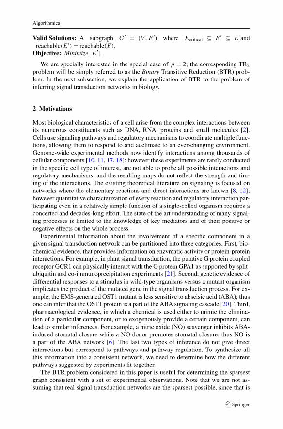
We now review the algorithm for finding the minimum weight spanning arbores-cence [3, 7, 16] since it will be necessary to modify it slightly later. Discard all in-coming edges to the root. Then the algorithm proceeds as follows. First, we selectfor each node, except the root, an incoming edge of minimum weight (breaking tiesarbitrarily). If these edges do not give a spanning arborescence, then there must bea directed cycle C formed by some of these edges. Let δC be the minimum of theweights of the edges in C. We contract C to a “supernode” and decrease the weightof every edge i → k from vertex i �∈ C to vertex k ∈ C by p − δC where p is theweight of the unique edge in C that is incoming to k. The process is then repeatedon the reduced graph, and continued until either we have a spanning arborescence onthe remaining graph. The supernodes are then expanded in reverse order. Each timea supernode is expanded, exactly one of its edges that would produce two incomingedges to a node is discarded. The same algorithm with minor modification can beused to find the reverse spanning arborescence rooted to v also. Figure 5 illustratesthe algorithm. Algorithm A2 can be implemented to run in O(min{|E| log |V |, |V |2})time; see [23] for details.

7.3 Augmenting and Combining the Two Algorithms

7.3.1 Augmenting Algorithm A1

Lemma 7 Algorithm A1 can be modified such that it solves the TRp problem on G

and uses at most 2.236α + 1.618β edges.

Proof We will show how to augment Algorithm A1 to handle

• A non-empty Ecritical and• A multiple parity component.

Algorithmica

Fig. 5 Illustration of the minimum weight spanning arborescence algorithm. The thick edges selected in acreate a cycle. The cycle is replaced by a supernode and the edge weights are adjusted in b. The thick edgesselected in b give a spanning arborescence on the remaining graph. When the supernode is expanded forthe final solution in c, one of the edges in the cycle is discarded

By Lemma 4(b), if G = (V ,E) is of multiple parity, we can find a simple cycle C

of non-zero parity whose addition to the solution of Algorithm A1 would providepaths of all parities between every pair of vertices. Let k be the constant used in thedescription of Algorithm A1. If |V | < k2, we can solve the problem in O(1) time.Otherwise, obviously |Eopt(G)| ≥ |E1

opt(G)| = α + β ≥ |V | = k2. If C contains k ormore edges, we can let C be the first cycle contracted by Algorithm A1. Otherwise,we just add the edges in C, if necessary, to the solution returned by Algorithm A1.With this modification, |E1| ≤ (1.617 + 1

k(k−1)+ 1

k)(α + β), or |E1| ≤ 1.618(α + β)

by appropriate choice of k.Now, we show how to handle the edges in Ecritical. We replace an edge u

x→ v ∈Ecritical by introducing a new vertex Xu,v and two new edges u

0→ Xu,v and

Xu,vx→ v. Let G′ = (V ′,E′) be the new graph. It is clear that all the new edges must

be selected by Algorithm A1 since otherwise either reachability from some Xu,v orreachability to some Xu,v will be violated. Moreover, there are exactly 2α new edges.Consider a solution returned by Algorithm A1 on G′. Then, we can contract the newedges to the original edges in G to get a solution E1 for G. Note that an optimalsolution for TR1 on G′ with no critical edges uses at most 2α + β edges since, inparticular, one solution of TR1 on G′ with no critical edges involves taking 2α newedges and β edges from E1

opt \ Ecritical. The contraction removes α edges from thissolution. Thus, the total number of edges selected with this modification is at most|E1| ≤ 1.618(2α + β) − α = 2.236α + 1.618β . �

7.3.2 Augmenting Algorithm A2

Lemma 8 Algorithm A2 can be modified such that it solves the TRp problem on G

and uses at most 2α + 2β + 1 edges.

Algorithmica

Proof We show how to augment Algorithm A2 to handle a multiple-parity graph.Again, by Lemma 4(b), we can find a simple cycle C of non-zero parity whose ad-dition to the solution of Algorithm A2 would provide paths of all parities betweenevery pair of vertices. Assume that at least one edge of C does not belong to Ecritical

since otherwise we do not incur any additional cost in adding C to our solution. Re-member that the first stage of Algorithm A2 starts by selecting one incoming edge ofminimum weight for every vertex. We will modify wt(e) for some edges e ∈ C suchthat Algorithm A2 starts by selecting all the edges in C and show that the additionalcost incurred is not too much. We classify each edge u → v ∈ C in the followingway:

(i) wt(u → v) = 0. We can then surely select this edge.(ii) wt(u → v) = 1 and every edge u′ → v has wt(u′ → v) = 1. Then also we can

select this edge.(iii) wt(u → v) = 1 and some edge u′ → v has wt(u′ → v) = 0. Then, we change

wt(u → v) to zero which would allow us to select this edge. Let S be the setof all these edges. Since wt(u′ → v) = 0 implies u′ → v ∈ Ecritical, |S| ≤ α andthus the total number of additional edges that appear in the solution of Algo-rithm A2 due to these changes is at most α.

(iv) When the supernode for C is expanded, all except one edge of C, say the edgeu → v, are selected. Thus, this edge which was not selected adds 1 to the countof additional edges.

Since we changed some edge weights from one to zero, the sum of edge weights inthe solution of Algorithm A2 does not increase. Thus, with this modification, we get|E2| ≤ 2(α + β) + 1. �

7.3.3 Combining Algorithms A1 and A2

1.78-approximation for TR1 for a Strongly Connected ComponentFor TR1 a strongly connected graph cannot be of multiple parity. In this case, our

solution is the better of the solutions provided by modified Algorithms A1 and A2without the modification. The approximation ratio is

ρ = min

{2.236α + 1.618β

α + β,α + 2β

α + β

}

= min

{2.236 + 1.618β

α

1 + βα

,1 + 2β

α

1 + βα

}

.

There are now two cases to consider.

Case 1. βα

≤ 1.1360.382 . Since

1+2 βα

1+ βα

increases with increasing βα

,

ρ ≤ 1 + 2 × 1.1360.382

1 + 1.1360.382

< 1.78.

Algorithmica

Case 2. βα

> 1.1360.382 . Since

2.236+1.618 βα

1+ βα

decreases with increasing βα

,

ρ ≤ 2.236 + 1.618 × 1.1360.382

1 + 1.1360.382

< 1.78.

2 + o(1)-approximation for TRp for a Strongly Connected ComponentIn this case, our solution is simply the output of modified Algorithm A2. Since

|E2| < 2(α + β) + 1 and |Emaxopt(G)| ≤ |E1opt(G)| = α + β ≤ |Eopt(G)|, |E2||Eopt(G)| ≤

2 + o(1).

7.4 Approximating TRp for General Graphs: Combining DAG and StronglyConnected Component Solutions

Now that we have an approximation algorithm for each strongly connected com-ponent and an exact algorithm for DAGs, how can we use these to design an ap-proximation algorithm for a general graph? First, we outline a general strategy forthis purpose. Then we show how to apply the strategy for single and multiple paritycomponents. The details of the strategy are somewhat different from that in [1, 13]because the strongly connected components can be of two types of parity.

Let G = (V ,E) be the given graph with C1 = (VC1 ,EC1),C2 = (VC2 ,EC2), . . . ,

Cm = (VCm,ECm) being the m strongly connected components where the ith com-ponent Ci contains ni vertices vi,1, vi,2, . . . , vi,ni

; thus

• ⋃mi=1 VCi

= V and∑m

i=1 ni = |V |;• V (Ci) ∩ V (Cj ) = ∅ if i �= j ;• ⋃m

i=1 E(Ci) ⊆ E.

By a gadget �i for the component Ci we mean a DAG of O(p2) edges on a new setof O(p) vertices. No two gadgets share a vertex.

Let C1,C2, . . . ,Cm be the connected components of G in an arbitrary orderand suppose that we have gadgets �1 = (V�1 ,E�1),�2 = (V�2 ,E�2), . . . ,�m =(V�m,E�m) for the components C1,C2, . . . ,Cm, respectively. Let Egadget = ∪m

i=1E�i

be the set of all edges in all the gadgets. For notational convenience let G0 = (V 0,E0)

be a graph identical to the given graph G; thus V 0 = V and E0 = E. Also, for no-tational convenience define e0 = {e} for every edge e ∈ E. Let G′ be a new graphobtained from G by a polynomial-time procedure Tcycle-to-gadget of the following na-ture:

• For i = 1,2, . . . ,m do the following:– The starting graph for the ith iteration is Gi−1.– The component Ci in Gi−1 is replaced by its corresponding gadget �i .– The edge replacement mapping is as follows:

∗ An edge e in Gi−1 with both end-points not in Ci stays the same, i.e., thereplacement of the edge is the edge itself.

∗ If Ci is a multiple parity component then we do the following.· For an incoming edge u

x→ v in Gi−1 from a vertex u not in Ci to a vertex v

in Ci the replacement is a set of p edges (a group of “first type” replaced

Algorithmica

edges) {u 0→ v′, u 1→ v′, . . . , u p−1→ v′} to some vertex v′ in �i . We will saythat the edge u

x→ v is the “corresponding edge” for these set of replacededges.

· Similarly, for an outgoing edge ux→ v in Gi−1 from a vertex u in Ci to a

vertex v not in Ci the replacement is a set of p edges (a group of “first

type” replaced edges) {u′ 0→ v,u′ 1→ v, . . . , u′ p−1→ v} from some vertex u′in �i . We will say that the edge u

x→ v is the “corresponding edge” for theseset of replaced edges.

∗ If Ci is a single parity component then we do the following.· For an incoming edge u

x→ v in Gi−1 from a vertex u not in Ci to avertex v in Ci the replacement is a set of p edges (a group of “second

type” replaced edges) {u 0→ v0, u1→ v1, . . . , u

p−1→ vp−1} to some vertices

v0, v1, . . . , vp−1 in �i . We will say that the edge ux→ v is the “correspond-

ing edge” for these set of replaced edges.· Similarly, for an outgoing edge u

x→ v in Gi−1 from a vertex u in Ci to avertex v not in Ci the replacement is a set of p edges (a group of “sec-

ond type” replaced edges) {u00→ v,u1

1→ v, . . . , up−1p−1→ v} from some

vertices u0, u1, . . . , up−1 in �i . We will say that the edge ux→ v is the “cor-

responding edge” for these set of replaced edges.∗ Let ei denote the union of replacements of all the edges in ei−1.

– The resultant graph at the end of the ith iteration is denoted by is Gi = (V i,Ei).• Remove identical groups of edges5 from Gm, i.e., if there are two groups of edges

em and f m with em = f m, remove one of the groups. Let G′ be the resulting graph.

Example 3 (Illustration of the notations in edge replacement) Suppose that the givengraph G has seven strongly connected components C1,C2, . . . ,C7, p = 2, the edgese1, e2 connect from a vertex in C1 to a vertex in C2, the edge e3 connect from a vertexin C2 to a vertex in C3, and let the edges {e4, e5, . . . , e9} have both endpoints fromC3,C4, . . . ,C7, i.e., for each edge e ∈ {e4, e5, e6, e7, e8, e9}, e connects two nodes u

and v such that u ∈ C and v ∈ C′ with C,C′ ∈ {C3,C4,C5,C6,C7}. Suppose that thereplacement step for C1 replaced the edge in e0

1 and e02 by a group of 2 second type

edges α,β and α′, β ′,respectively; the replacement step for C2 replaced the edge α

by a group of 2 first type edges γ, δ, replaced the edge β by a group of 2 second typeedges κ, ν, replaced the edge α′ by a group of 2 first type edges γ ′, δ′, replaced theedge β ′ by a group of 2 second type edges κ ′, ν′, and replaced the edge in e1

3 by agroup of 2 first type edges μ,θ . Then,

e01 = {e1}, e0

2 = {e2}, e03 = {e3}, e0

4 = {e4}, e05 = {e5},

e06 = {e6}, e0

7 = {e7}, e08 = {e8}, e0

9 = {e9},e1

1 = {α,β}, e12 = {α′, β ′}, e1

3 = {e3}, e14 = {e4}, e1

5 = {e5},

5Two groups em, f m of edges are identical iff there is a bijection H from em to f m such that, for e ∈ em

and f ∈ f m, H(e) = f iff e is an edge from u to v of parity x and f is an edge from u to v of parity x.

Algorithmica

e16 = {e6}, e1

7 = {e7}, e18 = {e8}, e1

9 = {e9},e2

1 = {γ, δ, κ, ν}, e22 = {γ ′, δ′, κ ′, ν′}, e2

3 = {μ,θ}, e24 = {e4},

e25 = {e5}, e2

6 = {e6}, e27 = {e7}, e2

8 = {e8}, e29 = {e9}.

Proposition 2 For any edge e ∈ E and any i, |ei | ≤ p2.

Proof Suppose that e connects the two components Cx and Cy with x < y. Then,

1 = |e0| = |e1| = · · · = |ex−1|,|ex | = p · |ex−1| = p,

p = |ex | = |ex+1| = · · · = |ey−1|,|ey | = p · |ey−1| = p2,

p2 = |ey | = |ey+1| = · · · = |em|. �

Proposition 3 G′ = Gm is a DAG.

Proof Consider the graph G′′ obtained by removing the edges in Egadget from G′.Since an edge in G between two connected components was replaced by a set ofedges between the same two connected components, G′′ specifies the interconnec-tions between strongly connected components and is therefore well-known to be aDAG (e.g., see [4]). Consider a topological ordering of the vertices of G′′ in whichall the vertices in V�i

are placed consecutively in some arbitrary order for each i; thisis possible since all the edges connecting two vertices in the same connected compo-nent were removed. Furthermore, since all the edges connecting two vertices in thesame connected component were removed, the topological ordering of the vertices ofG′′ is not destroyed if the vertices in V�i

in the above topological order are permutedin any arbitrary order as long as they are placed consecutively; thus we can rearrangethe vertices in V�i

, for each i, such that they are placed consecutively in an ordercorresponding to the topological sorting of the vertices of the DAG �i . Now, if weput back the missing edges of E�i

, for each i, in this topological sorting of G′′ wearrive at a topological sorting of G′. �

Now, we show that the graph G′ = Gm in fact satisfies the c-limited overlap prop-erty of Definition 1 for some constant c once we remove identical groups of edges.

Proposition 4 Let em1 , em

2 , . . . , emt be the non-identical groups of edges which make

up E′ = ⋃ti=1 em

i . Then, em1 , em

2 , . . . , emt define a c-limited partition of E′ for some

constant c.

Proof Note that two groups of edges em and f m have a non-empty intersection onlyif both e ∈ e0 and f ∈ f 0 are edges between the same pair of connected componentsin the given graph G. Since each connected component is replaced by O(p) verticesin the gadget, there are only O(p2) = O(1) edges between these two components.Each edge in e or f is one of these O(p2) = O(1) edges. �

Algorithmica

Example 4 (Illustration of the proof of Proposition 4) Consider Example 3 again.Since e1 and e2 are the only two edges that connect the same pair of connectedcomponents C1 and C2, e2

1 = {γ, δ, κ, ν} can have a non-empty intersection withe2

2 = {γ ′, δ′, κ ′, ν′} only and vice versa.

Abusing terminologies slightly, we now state what we mean by a “valid solution”for Gi .

Definition 9 By a “valid solution” for Gi , for i ∈ {0,1,2, . . . ,m}, we mean a validsolution of the grouped TRp problem on Gi when the edge groups are ei for eachedge e in the given graph G = G0 that connects two connected components. An“optimal solution” for Gi is a “valid solution” with a minimum number of edges.

Example 5 (Illustration of a valid solution for Gi ) Consider Example 3 again. By a“valid solution” for G2 = (V 2,E2) we mean a valid solution of the grouped TRp

problem for G2 where the edge partitions of E2 = {γ, δ, κ, ν, γ ′, δ′, κ ′, ν′,μ, θ, e4,

e5, e6, e7, e8, e9} are given by {γ, δ, κ, ν}, {γ ′, δ′, κ ′, ν′}, {μ,θ}, {e4}, {e5}, {e6}, {e7},{e8}, {e9}.

Note that a “valid solution” for G0 is obviously a valid solution of the TRp prob-lem on G since each group of edges in G = G0 consists of one single edge. SinceG′ is a DAG with c-limited overlap for some constant c, we can find an “opti-mal solution” for G′ exactly via the algorithm described in Lemma 2. Also, sup-pose the above procedure Tcycle-to-gadget guarantees the following invariants for eachi ∈ {1,2, . . . ,m}:(P 1i ) Any valid solution of TRp for Gi must contain all the edges in the gadget �i ,

and(P 2i ) If an edge u

x→ v to or from Ci was replaced by a set of first or second typeedges in Gi , then any valid solution for Gi either selects all of these edges orselects none of these edges.

Notice that our definition of a valid solution for Gi in Definition 9 trivially satisfiesthe Invariant (P 2i ). As an illustration, consider the illustration of a valid solutionin Example 5. A “valid solution” for G2 must contain all or none of the edges in{γ, δ, κ, ν}; this obviously implies that the solution contains all or none of the set ofedges in {γ, δ} and contains all or none of the set of edges in {κ, ν}. Thus, we do notneed to verify Invariant (P 2i ) at all.

Given an “optimal solution” E(m) ⊆ Em of the DAG G′ = Gm = (V m,Em)

with |E(m)| = OPT (G′), we associate it with a subgraph E(0) ⊆ E0 of G = G0 =(V 0,E0) via a procedure Tgadget-to-cycle in the following manner:

• For i = m,m − 1, . . . ,1 do the following:– Notice that E(i) is a subset of edges of Gi . We will maintain Invariant (�) de-

scribed subsequently that will ensure that E(i) is a “valid solution” of Gi .– Since E(i) is a “valid solution” of Gi , it satisfies Invariants (P 1i ) and (P 2i ).– Replace the vertices and edges of �i by the vertices and edges in an optimal

solution Eopt(Ci) of Ci .

Algorithmica

– Replace a group of first type edges {u 0→ v′, u 1→ v′, . . . , u p−1→ v′} incoming tosome vertex v′ in �i by their “corresponding edge” u

x→ v in Gi−1.

– Replace a group of first type edges {u′ 0→ v,u′ 1→ v, . . . , u′ p−1→ v} outgoingfrom some vertex u′ in �i by their “corresponding edge” u

x→ v in Gi−1.

– Replace a group of second type edges {u 0→ v0, u1→ v1, . . . , u

p−1→ vp−1} incom-

ing to some vertices v0, v1, . . . , vp−1 in �i by their “corresponding edge” ux→ v

in Gi−1.

– Replace a group of second type edges {u00→ v,u1

1→ v, . . . , up−1p−1→ v} out-

going from some vertices v0, v1, . . . , vp−1 in �i . by their “corresponding edge”

ux→ v in Gi−1.

– The replacement of any other edge is the edge itself.– The resultant set of edges is denoted by E(i − 1) ⊆ Ei−1.

Example 6 (Illustration of the reverse edge replacement) Consider the same exampledescribed in Example 3. Suppose that a “valid solution” E(2) for G2 contains all theedges e2

1 = {γ, δ, κ, ν}, none of the edges in e22 = {γ ′, δ′, κ ′, ν′}, none of the edges in

e23 = {μ,θ}, and other edges not in e2

1 ∪ e22 ∪ e2

3. Then the “valid solution” E(1) of G1

now contains the edges {α,β} plus the other edges in E(2) that are not in e21 ∪e2

2 ∪e23.

By Gapprox = (Vapprox,Eapprox) we denote the solution of TRp for G = G0 pro-duced by Tgadget-to-cycle when E(m) is an “optimal solution” Eopt(G

′) for the DAGG′. Suppose that the procedure Tgadget-to-cycle satisfies the following invariant for eachi ∈ {m − 1,m − 2, . . . ,0}:(�i ) if E(i + 1) is an “optimal solution” for Gi+1, then E(i) is an “optimal solution”

for Gi .

One problem in executing the procedure Tgadget-to-cycle is that we cannot even com-pute an optimal solution Eopt(Ci) for a strongly connected component Ci since theproblem is NP-hard. Nonetheless, we have seen in the previous section how to com-pute an approximate solution for a strongly connected component Ci . The followingproposition essentially states that, provided we satisfy the Invariants (P 1i ), (P 2i ) and(�i), the approximation ratio for each strongly connected component carries over tothe final solution E(0).

Proposition 5 Suppose that we have a ρ-approximation of TRp on each Ci for someρ > 1. Then, we can use the procedures Tcycle-to-gadget and Tgadget-to-cycle to design aρ-approximation of TRp on G.

Proof Suppose that we have a ρ-approximation of TRp for each Ci . Our simplemodification to the procedure Tgadget-to-cycle involves replacing each �i by this ap-proximate solution; in other words, we replace the step

“replace the vertices and edges of �i by the vertices and edges in an optimalsolution Eopt(Ci) of Ci”

Algorithmica

by the step

“replace the vertices and edges of �i by the vertices and edgesin the ρ-approximate solution of Ci”.

We call this modified procedure by Tapproximate-gadget-to-cycle. To differentiate theoutputs of Tapproximate-gadget-to-cycle from Tgadget-to-cycle we denote the solutionE(i) for Gi by Tgadget-to-cycle by E(i) itself and the solution E(i) for Gi byTapproximate-gadget-to-cycle by E(i)′.

Obviously, E(i)′ still remains a “valid solution” for Gi with this change. Note that|E(m)′| = |E(m)|. To prove our claim it suffices to show that |E(j)′| ≤ ρ · |E(j)| forany j ∈ {m− 1,m− 2, . . . ,0}. Notice that the only difference between Tgadget-to-cycleand Tapproximate-gadget-to-cycle in producing E(j) and E(j)′ is that the step

“replace the vertices and edges of �i by the vertices and edges in an optimalsolution Eopt(Ci) of Ci”

for i ∈ {m,m − 1,m − 2, . . . , j + 1} was replaced by the step

“replace the vertices and edges of �i by the vertices and edgesin the ρ-approximate solution of Ci”.

Thus,

∣∣∣∣∣E(j)′ \

j+1⋃

i=m

ECi

∣∣∣∣∣=

∣∣∣∣∣E(j) \

j+1⋃

i=m

ECi

∣∣∣∣∣,

∣∣∣∣∣E(j)′ ∩

(j+1⋃

i=m

ECi

)∣∣∣∣∣≤ ρ ·

∣∣∣∣∣E(j) ∩

(j+1⋃

i=m

ECi

)∣∣∣∣∣

and finally

|E(j)′| =∣∣∣∣∣E(j)′ \

j+1⋃

i=m

ECi

∣∣∣∣∣+

∣∣∣∣∣E(j)′ ∩

(j+1⋃

i=m

ECi

)∣∣∣∣∣

≤∣∣∣∣∣E(j) \

j+1⋃

i=m

ECi

∣∣∣∣∣+ ρ ·

∣∣∣∣∣E(j) ∩

(j+1⋃

i=m

ECi

)∣∣∣∣∣

≤ ρ ·(∣

∣∣∣∣E(j) \

j+1⋃

i=m

ECi

∣∣∣∣∣+

∣∣∣∣∣E(j) ∩

(j+1⋃

i=m

ECi

)∣∣∣∣∣

)

= ρ · |E(j)|. �

To summarize, what remains to be shown is the following:

for any arbitrary i ∈ {1,2, . . . ,m}, show that

• Procedure Tcycle-to-gadget satisfies Invariant (P 1i ) and• Tgadget-to-cycle satisfies Invariant (�i−1).

Algorithmica

But, how do we check the Invariant (�i−1) described above? Let E1 be a “validsolution” for Gi and suppose that the procedure Tgadget-to-cycle transformed E1 to asubset E2 of edges of Gi−1. Suppose that instead we could maintain the followingtwo invariants for each i ∈ {1,2, . . . ,m}:(P 3i ) If E1 is an “optimal solution” for Gi then E2 is a “valid solution” for Gi−1.(P 4i ) A subgraph that is an optimal solution Eopt(G) for Gi−1, after application of

the procedure Tcycle-to-gadget on the connected component Ci , is transformedto a subgraph Gmin = (Vmin,Emin) that is a valid solution for Gi .

To show that the above two invariants are sufficient to maintain instead of (�i−1), thefollowing proposition becomes useful.

Proposition 6 |Eopt(G) ∩ ECi| = |Eopt(Ci)| for a strongly connected component

Ci = (VCi,ECi

) and |Eopt(G′) ∩ E�i

| = |Eopt(�i)| for a gadget �i = (V�i,E�i

).

Proof We first prove the claim |Eopt(G) ∩ ECi| = |Eopt(Ci)|. This was essentially

observed in [1]. One can prove this in two parts as follows.

• We need to show that |Eopt(G) ∩ ECi| ≤ |Eopt(Ci)|. Suppose that this is not true

and hence |Eopt(G) ∩ ECi| > |Eopt(Ci)|. But then (Eopt(G) \ (Eopt(G) ∩ ECi

)) ∪Eopt(Ci) gives another solution with fewer edges than in Eopt(G).

• We need to show that |Eopt(G) ∩ ECi| ≥ |Eopt(Ci)|. Suppose that this is not true

and hence |Eopt(G)∩ECi| < |Eopt(Ci)|. This implies that there is a pair of vertices

u and v in Ci such that there is a path u ⇒ v from u to v that includes a vertexw not in Ci as an intermediate vertex. But this implies that w should be in thestrongly connected component Ci , a contradiction.

|Eopt(G′) ∩ E�i

| = |Eopt(�i)| is true since we maintain Invariant (P 1i ). �

Now, we claim the following.

Proposition 7 If we satisfy Invariant (P 1i ) then Invariants (P 3i ) and (P 4i ) implyInvariant (�i−1).

Proof It suffices to show that if we satisfy Invariants (P 3i ) and (P 4i ) then E2 is anoptimal solution for Gi−1.

We first show the proof for i = m. The same proof with minor modifications canbe applied for i = m − 1,m − 2, . . . ,1, in that order, to complete the proof of thisproposition.

For every 1 ≤ q �= r ≤ m, let Eiq,r be those edges in ∪e∈Ei {e} that connect a vertex

in Cq (or �q if Cq was already replaced by �q in Gi ) to a vertex in Cr (or �r if Cr

was already replaced by �r in Gi ).For a pair of q and r , consider the set of edges in E1 ∩ Em

q,r . Note that there isno edge common between the set of edges E1 ∩ Em

q,r and E1 ∩ Emq ′,r ′ if either q �= q ′

or r �= r ′. Remember that in the proof of Lemma 2, we actually showed that anyvalid solution must contain a subset Em′

q,r of the edges in E1 ∩ Emq,r and the rest of

the edges in E1 ∩ Emq,r come from a minimum collection of groups of edges from

Algorithmica

Emq,r that included the edges in this subset. Suppose that the procedure Tgadget-to-cycle

mapped the edges in Em′q,r to a subset E

(m−1)′q,r of edges in Em−1

q,r . We claim that any

valid (and thus optimal) solution of Gm−1 must contain the edges in E(m−1)′q,r . Indeed,

for the sake of contradiction, suppose that it is not so. Then, such an optimal solution

does not contain an edge e ∈ E(m−1)′q,r and applying the procedure Tcycle-to-gadget on

this valid solution for Gm−1 creates a subset of edges in Em that does not includeat least one edge from Em′

q,r . By (P 4i ) this subset of edges must be a valid solutionof Gm but this is not possible since every valid solution of Gm must include all theedges in Em′

q,r .

Now, to show that E2 is indeed an optimal solution for Gm−1, all we need to show

is that the rest of the edges in E2 ∩ Em−1q,r that do not belong to E

(m−1)′q,r come from a

minimum collection of groups of edges from Em−1q,r that include the edges in E

(m−1)′q,r .

Indeed, suppose that it is not so and let a valid solution for Gm−1 contain another

subset E′2 of Em−1

q,r that include the edges in E(m−1)′q,r , |E′

2| < |E2|, and applying

the procedure Tcycle-to-gadget on this valid solution creates a subset E′1 of Em−1

q,r that

include the edges in Em′q,r . Note that the procedure Tcycle-to-gadget replaces every edge

of either first or second type in Gm−1 by exactly p edges in Gm. Thus, |E1| = p ·|E2|, |E′

1| = p · |E′2| and |E′

2| < |E2| implies |E′1| < |E1| contradicting the optimality

of E1.The same proof can be carried out for i = m−1,m−2, . . . ,1, in that order, except

that the line in the proof

“Remember that in the proof of Lemma 2, we actually showed that any validsolution must contain a subset Em′

q,r of the edges in E1 ∩Emq,r and the rest of the

edges in E1 ∩ Emq,r come from a minimum collection of groups of edges from

Emq,r that included the edges in this subset”

should be slightly changed to

“Remember that in the proof of this proposition for i + 1 that precedes theproof for i, we actually showed that any valid solution must contain a subsetEi′

q,r of the edges in E1 ∩Eiq,r and the rest of the edges in E1 ∩Ei

q,r come froma minimum collection of groups of edges from Ei

q,r that included the edges inthis subset”

and the rest remains essentially the same. �

Example 7 (Example illustrating the proof of Proposition 7) Consider the examplein Example 3 again. Suppose that the edge γ is identical to the edge γ ′ and the edgeκ is identical to the edge κ ′; thus, we have

• E21,2 = {γ, δ, κ, ν, δ′, ν′};

• E11,2 = {α,β,α′, β ′}.

Suppose that E2′1,2 = {γ }. Then, one possible minimal way to cover E2′

1,2 is by the

group {γ, δ, κ, ν}; thus suppose that E1 ∩ E21,2 = {γ, δ, κ, ν}. Then, E1′

1,2 = {α} and

Algorithmica

E2 ∩ E11,2 = {α,β}. Moreover, if there was another way to cover the edge α in G1

with fewer than 2 edges that would have led to covering the edge γ with fewer than4 edges.

Note that the Invariants (P 1i ), (P 3i ) and (P 4i ) involve only the graphs Gi−1 and Gi ,the procedure Tcycle-to-gadget transforms Gi−1 to Gi by replacing only one stronglyconnected component Ci and the procedure Tgadget-to-cycle transforms a solution ofGi to a solution of Gi−1. Hence, we can simplify our notations by dropping thesubscripts/superscripts and paraphrasing our requirement as follows (abusing the no-tation for G slightly):

• We are given a graph G = (V ,E) that contains at least one strongly connectedcomponent of either single or multiple parity.

• The procedure Tcycle-to-gadget, as described in detail before, replaces just one ar-bitrarily strongly connected component, say C = (VC,EC), of G to transforms G

to G′ = (V ′,E′). The definition of a valid solution for G′ includes the additionalconstraint that if an edge u

x→ v to or from C was replaced by a set of first or sec-ond type edges in G′, then a valid solution for G′ must either select all of theseedges or select none of these edges. Let � = (V�,E�) be the gadget for C. Thisprocedure must satisfy the following invariant:

(P 1) any “valid solution” for G′ must contain all the edges in the gadget �, and

• The procedure Tgadget-to-cycle, as described in details before, transforms an optimalE1 ⊆ E′ solution of G′ to a solution E2 ⊆ E of G. This procedure must satisfy thefollowing invariant:

(P 3) If E1 is an “optimal solution” for G′ then E2 is a “valid solution” for G.(P 4) A subgraph that is an optimal solution Eopt(G) for G, after application of

the procedure Tcycle-to-gadget on the connected component C, is transformedto a subgraph Gmin = (Vmin,Emin) that is a valid solution for G′.

The above rephrasing makes it clear that it suffices to show that invariants aremaintained when just one strongly connected component is replaced. Our entire dis-cussion then summarizes to state that if we can design the procedures Tcycle-to-gadgetand Tgadget-to-cycle as stated above then a ρ-approximation of TRp for a strongly con-nected graph implies a ρ-approximation of TRp for general graphs.

Finally, note that due to Proposition 6, the fact that Invariant (P 1) ensures thatall the edges in the gadget � for the component C are selected in any valid solutionfor G′ and the fact that the procedure Tgadget-to-cycle replaces the gadget by a validsolution for C, when checking for Invariants (P 3) or (P 4), we need to check only forthose paths u

x⇒ v in G such that u and v do not belong to the same component andthose paths u

x⇒ v in G′ such that u and v do not belong to the same gadgets in G′.In the next two sections, we consider the two cases corresponding to whether C is

of multiple parity or single parity and show that the invariants are satisfied.

7.4.1 Handling Strongly Connected Components of Multiple Parity

Note that by definition a multiple parity component must have at least 2 vertices.The component C corresponds to a gadget � in the following manner. We introduce

Algorithmica

Fig. 6 Gadget � for a multiple parity component C for the TR2 problem. Due to Invariant (P 2), bothor none of the edges in each of the following pairs of edges will be selected in a “valid solution” for G′:{u 0→ XC,u

1→ XC }, {v 0→ XC,v1→ XC }, {XC

0→ u′,XC1→ u′} and {XC

0→ v′,XC1→ v′} by u

0,1→ XC ,

v0,1→ XC , XC

0,1→ u′ , XC0,1→ v′

one new vertex XC . An incoming edge in G to some vertex in C now becomes p

incoming edges of parities 0,1, . . . , p − 1 to XC and an outgoing edge from somevertex in C now becomes p outgoing edges from XC of parities 0,1, . . . , p − 1.Figure 6 illustrates the gadget for p = 2.

We need to verify the invariants (P 1), (P 3) and (P 4). (P 1) vacuously holds.To verify (P 3), one must consider the following cases.

(I) ux⇒ v is in G when u ∈ VC and v �∈ VC . Suppose that u′ is the last vertex on

this path that belongs to C; thus the path is of the form ux1⇒ u′ x2→ v′ x3⇒ v.

Thus XC

x2⊕px3�⇒ v exists in Eopt(G′). Suppose that this path translates to the

path u′′ x2⊕px3�⇒ v in Gapprox for some u′′ ∈ C. Since uz⇒ u′′ exists in C for every

z ∈ {0,1, . . . , p − 1}, we have the path ux⇒ v in Gapprox.

(II) ux⇒ v is in G when u �∈ VC and v ∈ VC . Similar to (I).

(III) ux⇒ v is in G when u,v �∈ VC but the path contains at least one vertex from

VC . Let ux1⇒ u′ x2⇒ v′ x3⇒ v where u′ and v′ are the first and the last vertices

that belong to C. But, then ux1⇒ u′ and v′ x3⇒ v exist in Gapprox by (I) and (II),

respectively, and u′ x2⇒ v′ exist in Gapprox since C is a multiple parity componentand Tgadget-to-cycle replaced every XC by Eopt(C).

To verify (P 4), one must consider the following cases.

(I) XC ⇒ v is in G′. Since every outgoing edge from XC has parity z for everyz ∈ {0,1,2, . . . , p − 1}, XC

z⇒ v exists in G′ each z ∈ {0,1,2, . . . , p − 1}. Pick

any vertex u ∈ C. Obviously, u0⇒ v = u

x1⇒ u′ x2→ v′ x3⇒ v exists in Eopt(G)

where u′ is the last vertex on the path that is in C. Then, both XC{0,1,2,...,p−1}−→ v′

and v′ x3⇒ v are in Gmin.(II) v ⇒ XC is in G′. Similar to (I).

(III) u ⇒ XC ⇒ v is in G′. Follows from (I) and (II) since both u ⇒ XC and XC ⇒ v

are in Gmin.

Algorithmica

7.4.2 Handling Strongly Connected Components of Single Parity

Let v be any vertex in the single parity component C = (VC,EC). Define the follow-ing notation:

[j ] = {x ∈ VC |v j⇒ x exists in C}.Note that for any u,v ∈ VC , u

x⇒ v is in C if and only if vp−x�⇒ u is in C since

otherwise uy⇒ u is in C for some y ∈ {1,2, . . . , p − 1} which is not allowed due to

Lemma 4(b).

Lemma 10 For any u ∈ [i] and u′ ∈ [j ], ux⇒ u′ if and only if x =p j − i.

Proof Consider the path up−i�⇒ v

j⇒ u′ and note that there are paths of only one paritybetween any two vertices in a single parity component. �

Via the above lemma, we can design the following gadget � for the single paritycomponent C = (VC,EC):

• The new vertices and edges in � are as follows:– The set of new vertices are

⋃p−1i=0 {[i]′, [i]′′};

– For each [i]′ ∈ {[0]′, [1]′, . . . , [p − 1]′} and [j ]′′ ∈ {[0]′′, [1]′′, . . . , [p − 1]′′},there is an edge [i]′ x→ [j ]′′ where x =p j − i.

• An incoming edge u′ x→ u to C with u′ �∈ VC and u ∈ VC is mapped byTcycle-to-gadget to the following set of edges:

Case Corresponding set of second-type edges Reference

u ∈ [j ] u′ x⊕p��pj→ [�]′ for each � ∈ {0,1, . . . , p − 1} (Cj,x,u′)′

• An outgoing edge ux→ u′ from C with u′ �∈ VC and u ∈ VC is mapped by

Tcycle-to-gadget as shown below:

Case Corresponding set of second-type edges Reference

u ∈ [j ] [�]′′ x⊕pj�p�→ u′ for each � ∈ {0,1, . . . , p − 1} (Cj,x,u′)′′

• Finally, if any pair of constraints (Cj1,x1,u1)′, (Cj2,x2,u2)

′ or (Cj1,x1,u1)′′,

(Cj2,x2,u2)′′ generate the same set of edges, we remove one of the sets.

As a specific illustration, consider the graph on the top of Fig. 7 for the TR2 problem;the corresponding gadget is shown below.

The following properties of gadget edges will be useful.

Lemma 11 The following statements are true:

(a) [j ]′′ y→ u′ with u′ �∈ VC is in G′ implies that, for every 0 ≤ � < p, [�]′′ y⊕pj�p�−→ u′

is also in G′. Moreover, the edge [�]′′ y′→ u′ is an edge among the set of edges in

(Cj,y′⊕p��pj,u′) for exactly one 0 ≤ j < p.

Algorithmica

Fig. 7 Gadget � for a single parity component C for an instance of the TR2 problem.[0] = {v1, v3, v5, v6}, [1] = {v2, v4}

(b) u′ y→ [j ]′ with u′ �∈ VC is in G′ implies that, for every 0 ≤ � < p, u′ y⊕p��pj−→ [�]′is also in G′. Moreover, the edge u′ y′

→ [�]′ is an edge among the set of edges in(Cj,y′�p�⊕pj,u′) for exactly one 0 ≤ j < p.

Proof (a) Suppose that the edge [j ]′′ y→ u′ was introduced by the edge wx→ u′ of

G with w ∈ [t] under the constraint (Ct,x,u′)′′. Thus, y =p x + t − j . The same

constraint also generated the edge [�]′′ y′→ u′ where y′ =p x + t − � =p y + j − �.

For the second part, note that two constraints (Cj1,y′⊕p��pj1,u′) and(Cj2,y′⊕p��pj2,u′) generate the same set of edges and hence one of them will beremoved.

(b) Suppose that the edge u′ y→ [j ]′ was introduced by the edge u′ x→ w of G withw ∈ [t] under the constraint (Ct,x,u′)′. Thus, y =p x + j − t . The same constraint

also generated the edge u′ y′→ [�]′ where y′ =p x + � − t =p y + � − j .

For the second part, note that two constraints (Cj1,y′�p�⊕pj1,u′) and(Cj2,y′�p�⊕pj2,u′) generate the same set of edges and hence one of them will beremoved. �

We need to verify Invariants (P 1), (P 3) and (P 4). (P 1) obviously holds. It nowremains to verify the invariants (P 3) and (P 4)

To verify (P 3), one must consider the following cases.

(I) ux⇒ w is in G when u ∈ C and w �∈ C. Suppose that u′ is the last vertex on this

path that belongs to C. Thus the path is of the form ux1⇒ u′ x2→ w′ x3⇒ w with

x =p x1 + x2 + x3. Suppose that u ∈ [r] and thus u′ ∈ [s] where s =p r + x1.

Eopt(G′) contains the path [s]′′ x2⇒ w′ x3⇒ w since the edge [s]′′ x2→ w′ exists in

G′. Suppose that Tgadget-to-cycle translated this path to a path u′′ x2⊕ps�pt�⇒ w′ x3⇒

Algorithmica

w for some u′′ ∈ [t]. Then the path ux1⇒ u′ t�ps�⇒ u′′ x2⊕ps�pt�⇒ w′ x3⇒ w is of parity

x.(II) w

x⇒ u is in G when u ∈ C and w �∈ C. Similar to (I).(III) u

x⇒ w is in G when u,w �∈ C but the path contains at least one vertex in C. Letu

x1⇒ u′ x2⇒ v′ x3⇒ w where u′ and v′ are the first and the last vertices that belongto C. But, then u

x1⇒ u′ and v′ x3⇒ w exist in Gapprox by (I) and (II), respectively,

and u′ x2⇒ v′ exist in Gapprox because of the gadget edges.

Now we turn our attention to the verification of (P 4). We know that in Gmin In-variant (P 2) is not violated for any (Cj,x,u)′ or (Cj,x,u)′′. Since all the gadget edgesare selected in any valid solution for G′, to verify (P 4) one needs to consider thefollowing cases.

(I) [i]′′ x→ w is in G′ for w �∈ ⋃p−1i=0 {[i]′, [i]′′}. By Lemma 11(a) this implies

that Eopt(G) contains ux⊕pi�pj�⇒ w for some u ∈ [j ]. Suppose that this path

is of the form uy1⇒ w′ y2⇒ w′′ x⊕pi�pj�py1�py2�⇒ w where w′ is the last vertex

on the path that belongs to C. By Lemma 10 w′ ∈ [j ⊕p y1]. Thus, the path

w′ y2�⇒ w′′ x⊕pi�pj�py1�py2�⇒ w in Eopt(G) translates to the path [j ⊕p y1]′′ y2�⇒w′′ x⊕pi�pj�py1�py2�⇒ w. By Lemma 11(a) the edge [j ⊕p y1]′′ y2�⇒ w′′ implies

that the edge [i]′′ j⊕py1�pi⊕py2�⇒ w′′ also exists and, by Invariant (P 2), selected

in Gmin. Then the path [i]′′ j⊕py1�pi⊕py2�⇒ w′′ x⊕pi�pj�py1�py2�⇒ w is of parity x.(II) w

x→ [i] is in G′ for w �∈ ⋃p−1i=0 {[i]′, [i]′′}. Similar to (I).

(III) w1x1→ [i] j�pi→ [j ] x2→ w2 is in G′ for w1,w2 �∈ ⋃p−1

i=0 {[i]′, [i]′′}. w1x1⇒ [i] and

[j ] x2⇒ w4 exist in Gmin by (II) and (I), respectively, and [i] j�pi→ [j ] is providedby one of the gadget edges for C.

Acknowledgements We wish to thank the anonymous reviewer for very helpful comments that led tosignificant improvements in the presentation of the paper. The second author would like to thank SamirKhuller for pointing out to him that the results in reference [9] provided a 2-approximation for TR1.

References

1. Aho, A., Garey, M.R., Ullman, J.D.: The transitive reduction of a directed graph. SIAM J. Comput.1(2), 131–137 (1972)

2. Alberts, B.: Molecular Biology of the Cell. Garland, New York (1994)3. Chu, Y., Liu, T.: On the shortest arborescence of a directed graph. Sci. Sin. 4, 1396–1400 (1965)4. Cormen, T.H., Leiserson, C.E., Rivest, R.L., Stein, C.: Introduction to Algorithms. MIT Press, Cam-

bridge (2001)5. DasGupta, B., Enciso, G.A., Sontag, E.D., Zhang, Y.: Algorithmic and complexity results for decom-

positions of biological networks into monotone subsystems. In: 5th International Workshop Experi-mental Algorithms. LNCS, vol. 4007, pp. 253–264. Springer, Berlin (2006)

6. Desikan, R., Griffiths, R., Hancock, J., Neill, S.: A new role for an old enzyme: nitrate reductase-mediated nitric oxide generation is required for abscisic acid-induced stomatal closure in Arabidopsisthaliana. Proc. Natl. Acad. Sci. USA 99, 16314–16318 (2002)

Algorithmica

7. Edmonds, J.: Optimum branchings. In: Dantzig, G.B. (ed.) Mathematics and the Decision Sciences,Part 1. Am. Math. Soc. Lectures Appl. Math., vol. 11, pp. 335–345. Am. Math. Soc., Providence(1968)

8. Fall, C.P., Marland, E.S., Wagner, J.M., Tyson, J.J.: Computational Cell Biology. Springer, New York(2002)

9. Frederickson, G.N., JàJà, J.: Approximation algorithms for several graph augmentation problems.SIAM J. Comput. 10(2), 270–283 (1981)

10. Giot, L., Bader, J.S., et al.: A protein interaction map of Drosophila melanogaster. Science 302, 1727–1736 (2003)

11. Han, J.D., Bertin, N., et al.: Evidence for dynamically organized modularity in the yeast protein-protein interaction network. Nature 430, 88–93 (2004)

12. Heinrich, R., Schuster, S.: The Regulation of Cellular Systems. Chapman & Hall, New York (1996)13. Khuller, S., Raghavachari, B., Young, N.: Approximating the minimum equivalent digraph. SIAM J.

Comput. 24(4), 859–872 (1995)14. Khuller, S., Raghavachari, B., Young, N.: On strongly connected digraphs with bounded cycle length.

Discrete Appl. Math. 69(3), 281–289 (1996)15. Khuller, S., Raghavachari, B., Zhu, A.: A uniform framework for approximating weighted connectiv-

ity problems. In: 19th Annual ACM-SIAM Symposium on Discrete Algorithms, pp. 937–938, 199916. Lawler, E.: Combinatorial Optimization: Networks and Matroids. Dover, New York (2000)17. Lee, T.I., Rinaldi, N.J., et al.: Transcriptional regulatory networks in Saccharomyces cerevisiae. Sci-

ence 298, 799–804 (2002)18. Li, S., Armstrong, C.M., et al.: A map of the interactome network of the metazoan C. elegans. Science

303, 540–543 (2004)19. Li, S., Assmann, S.M., Albert, R.: Predicting essential components of signal transduction networks: a

dynamic model of guard cell signaling. PLoS Biology 4(10) (October 2006)20. Mustilli, A.C., Merlot, S., Vavasseur, A., Fenzi, F., Giraudat, J.: Arabidopsis OST1 protein kinase

mediates the regulation of stomatal aperture by abscisic acid and acts upstream of reactive oxygenspecies production. Plant Cell 14, 3089–3099 (2002)

21. Pandey, S., Assmann, S.M.: The Arabidopsis putative G protein-coupled receptor GCR1 interactswith the G protein alpha subunit GPA1 and regulates abscisic acid signaling. Plant Cell 16, 1616–1632 (2004)

22. Sontag, E.D.: Some new directions in control theory inspired by systems biology. Syst. Biol. 1, 9–18(2004)

23. Tarjan, R.: Finding optimum branchings. Networks 7, 25–35 (1977)