Mathematical Programming manuscript No.(will be inserted by the editor)

R. Andreani · J. J. Judice · J. M.Martınez · J. Patrıcio

On the natural merit function forsolving complementarity problems ⋆

Received: 01/10/2007 / Accepted: date

Abstract Complementarity problems may be formulated as nonlinear sys-tems of equations with non-negativity constraints. The natural merit functionis the sum of squares of the components of the system. Sufficient conditionsare established which guarantee that stationary points are solutions of thecomplementarity problem. Algorithmic consequences are discussed.

Keywords Complementarity Problems · Merit functions · NonlinearProgramming

Mathematics Subject Classification (2000) 78M50 · 90C30

⋆ Research of J. J. Judice and J. Patrıcio was partially supported by ProjectPOCI/MAT/56704/2004 of the Portuguese Science and Technology Foundation. J.M. Martınez and R. Andreani were supported by FAPESP and CNPq (Brazil).

R. AndreaniInstituto de Matematica, Estatıstica e Computacao Cientıfica, Universidade Estad-ual de Campinas, BrazilE-mail: andreani@ime.unicamp.br

J. J. JudiceDepartamento de Matematica da Universidade de Coimbra, and Instituto de Tele-comunicacoes, Portugal.E-mail: Joaquim.Judice@co.it.pt

J. M. MartınezInstituto de Matematica, Estatıstica e Computacao Cientıfica, Universidade Estad-ual de Campinas, Brazil.E-mail: martinez@ime.unicamp.br

J. PatrıcioInstituto Politecnico de Tomar, and Instituto de Telecomunicacoes, Portugal.E-mail: Joao.Patricio@aim.estt.ipt.pt

2 R. Andreani et al.

1 Introduction

The Complementarity Problem (CP) considered in this paper consists of find-ing x,w ∈ Rn and y ∈ Rm such that

H(x, y, w) = 0, x⊤w = 0, x, w ≥ 0, (1)

where H : Rn+m+n −→ Rn+m is continuously differentiable on an open setthat contains Ω, and

Ω =(x, y, w) ∈ Rn+m+n : x,w ≥ 0

. (2)

The most popular particular case of (1) is the Linear ComplementarityProblem (LCP). In this case,

H(x,w) = Mx− w + q,

where M ∈ Rn×n and q ∈ Rn are given. Many applications of the LCP havebeen proposed in science, engineering and economics [9,14,17,22,23,29].

If G : Rn −→ Rn and H(x,w) = G(x) − w, the CP reduces to theNonlinear Complementarity Problem [14]. Furthermore, let

K = x ∈ Rn : h(x) = 0, x ≥ 0

where h : Rn −→ Rm is a continuously differentiable function on Rn. Wedenote ∇h(x) = (∇h1(x), . . . ,∇hm(x)). Then, under a suitable constraintqualification, defining

H(x, y, w) = ((G(x) +∇h(x)y − w)⊤, h(x)⊤)⊤, (3)

the CP problem turns to be equivalent to the Variational Inequality problemdefined by the operator G over K [1,14,33]. In particular, if G is the gradientof a continuously differentiable function f : Rn −→ R1, then CP with Hgiven by (3) represents the KKT conditions of the optimization problemdefined by minimizing f on the set K [14].

The formulation (1) is more general than (3), since there is no restric-tion on the form of the function H . For example, H may involve the KKTequations of a parametric optimization problem and, additionally, nonlinearconditions involving variables, multipliers and parameters.

Many reformulations of complementarity and variational inequality prob-lems have been discussed in the literature. See, for example, [2,3,11–15,18,20,21,25,28,35] and references therein. Some reformulations use the fact that[xiwi = 0, xi ≥ 0, wi ≥ 0] may be expressed as ϕ(xi, wi) = 0 by means ofthe so called NCP functions. The best known one is the Fischer-Burmeisterfunction [19]. As a consequence, complementarity problems may be writtenas nonlinear systems of equations and Newtonian ideas may be employedfor their resolution [18]. In the process os stating nonlinear complementar-ity problems and variational inequality problems as unconstrained nonlinearsystems of equations based on NCP functions, several authors proved equiv-alence between stationary points of the merit functions and solutions of theoriginal problem under different problem assumptions that go from strict

Merit function for complementarity 3

monotonicity to P0-like conditions. See [11,12,25,15]. Reformulations withsimple constraints based on the Fischer-Burmeister function with equivalenceresults were also proposed in [13].

In the present contribution, we consider the reformulation of CP as theproblem of finding a solution (x, y, w) ∈ Ω of the square nonlinear system

H(x, y, w) = 0, x1w1 = 0, . . . , xnwn = 0. (4)

The natural merit function [16,28] is introduced in Section 2, where suf-ficient conditions are proved ensuring that (first-order) stationary points ofthe corresponding bound-constrained minimization problem are solutions of(4). Algorithmic consequences of this approach are discussed.

Notation

The set of natural numbers is denoted by N.The symbol ‖ · ‖ denotes the Euclidean norm.

2 The Complementarity Problem and the natural merit function

Let us define F : Rn+m+n −→ Rn+m+n and f : Rn+m+n −→ R by

F (x, y, w) = (H(x, y, w)⊤, x1w1, . . . , xnwn)⊤

andf(x, y, w) = ‖F (x, y, w)‖2. (5)

We consider the problem

Minimize f(x, y, w) subject to (x, y, w) ∈ Ω, (6)

where Ω is given by (2).

We denote z = (x, y, w) from now on. Next we show that, if a stationarypoint (x, y, w) of (6) is not a solution of the complementarity problem (1),then the Jacobian matrix F ′(x, y, w) is singular. When one tries to solve anonlinear system F (x, y, w) = 0 with (x, y, w) ∈ Ω using a standard bound-constraint minimization solver, the main reason for possible failure is theconvergence to “bad” stationary points of (6) (generally local minimizers).Therefore, it is interesting to characterize the set of stationary points thatare not solutions of the system. In the following theorem, we show thatthis set is reasonably small in the sense that all its elements have singularJacobians. Note that this property is not true for general nonlinear systems.For example, for the system given by x+1 = 0, w− 1 = 0, the point (0, 1) isstationary but the Jacobian is obviously nonsingular. Therefore, the propertyproved below is a peculiarity of the complementarity structure of F .

Theorem 1 Suppose that z = (x, y, w) is a stationary point of (6). Then, if‖F (x, y, w)‖ 6= 0, the Jacobian F ′(x, y, w) is singular.

4 R. Andreani et al.

Proof Since the existence of the variables yi does not introduce any compli-cation to the proof, in order to simplify the notation, we only consider thecase in which z = (x,w) and F (z) = F (x,w).

Let (x,w) be a stationary point of f over Ω. If xi = wi = 0, for somei ∈ 1, . . . , n, then row n + i of the Jacobian is null, and the Jacobian issingular. Therefore the theorem is trivial in this case.

Assume that xik , wik > 0 for p indices ik, k = 1, . . . , p belonging to1, . . . , n. Then there are three possible cases:

Case 1: p = n;Case 2: p = 0;Case 3: 1 ≤ p < n.

In Case 1, the derivatives of f with respect to all the variables must vanish.Since

∇f(z) = 2F ′(z)⊤F (z),

this implies the desired result.Let us now consider Case 2. Since xi+wi > 0 for all i = 1, . . . , n, we may

assume without loss of generality that

xi = 0, wi > 0

for all i = 1, . . . , n. The Jacobian may be written as follows:

F ′(x,w) =

∂H∂x1

. . . ∂H∂xn

∂H∂w1

. . . ∂H∂wn

w1 . . . 0 x1 . . . 0...

. . ....

.... . .

...0 . . . wn 0 . . . xn

,

where∂H

∂xj

,∂H

∂wj

∈ Rn

for j = 1, . . . , n. Therefore at (x,w) we have

F ′(x,w) =

∂H∂x1

(x,w) . . . ∂H∂xn

(x,w) ∂H∂w1

(x,w) . . . ∂H∂wn

(x,w)

w1 . . . 0 0 . . . 0...

. . ....

.... . .

...0 . . . wn 0 . . . 0

. (7)

By stationarity, the derivatives of f with respect to wj must vanish. Hence,by (7),

H(x,w)⊤∂H

∂wj

(x,w) = 0

for all j = 1, . . . , n. Therefore, either H(x,w) = 0 or the vectors∂H∂w1

(x,w), . . . , ∂H∂wn

(x,w) are linearly dependent. By (7), the latter case im-

plies the singularity of the Jacobian. On the other hand, if H(x,w) = 0then F (x,w) = 0, due to the complementarity assumption (xiwi = 0 for alli = 1, . . . , n).

Merit function for complementarity 5

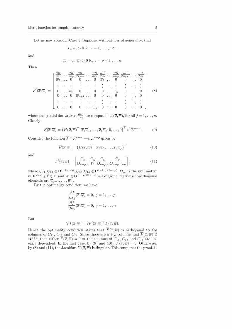
Let us now consider Case 3. Suppose, without loss of generality, that

xi, wi > 0 for i = 1, . . . , p < n

andxi = 0, wi > 0 for i = p+ 1, . . . , n.

Then

F ′(x,w) =

∂H∂x1

. . . ∂H∂xp

∂H∂xp+1

. . . ∂H∂xn

∂H∂w1

. . . ∂H∂wp

∂H∂wp+1

. . . ∂H∂wn

w1 . . . 0 0 . . . 0 x1 . . . 0 0 . . . 0...

. . ....

.... . .

......

. . ....

.... . .

...0 . . . wp 0 . . . 0 0 . . . xp 0 . . . 00 . . . 0 wp+1 . . . 0 0 . . . 0 0 . . . 0...

. . ....

.... . .

......

. . ....

.... . .

...0 . . . 0 0 . . . wn 0 . . . 0 0 . . . 0

(8)

where the partial derivatives ∂H∂wj

are computed at (x,w), for all j = 1, . . . , n.

Clearly

F (x,w) =(H(x,w)⊤, x1w1, . . . , xpwp, 0, . . . , 0

)⊤∈ Rn+n. (9)

Consider the function F : Rn+n −→ Rn+p given by

F (x,w) =(H(x,w)⊤, x1w1, . . . , xpwp

)⊤(10)

and

F ′(x,w) =

[C11 C12 C13 C14

On−p,p W On−p,p On−p,n−p

], (11)

where C11, C13 ∈ R(n+p)×p, C12, C14 ∈ R(n+p)×(n−p), Ojk is the null matrix

inRj×k, j, k ∈ N andW ∈ R(n−p)×(n−p) is a diagonal matrix whose diagonalelements are wp+1, . . . , wn.

By the optimality condition, we have

∂f

∂xj

(x,w) = 0, j = 1, . . . , p,

∂f

∂wj

(x,w) = 0, j = 1, . . . , n

But∇f(x,w) = 2F ′(x,w)⊤F (x,w),

Hence the optimality condition states that F (x,w) is orthogonal to thecolumns of C11, C13 and C14. Since these are n + p columns and F (x,w) ∈Rn+p, then either F (x,w) = 0 or the columns of C11, C13 and C14 are lin-early dependent. In the first case, by (9) and (10), F (x,w) = 0. Otherwise,by (8) and (11), the Jacobian F ′(x,w) is singular. This completes the proof.

6 R. Andreani et al.

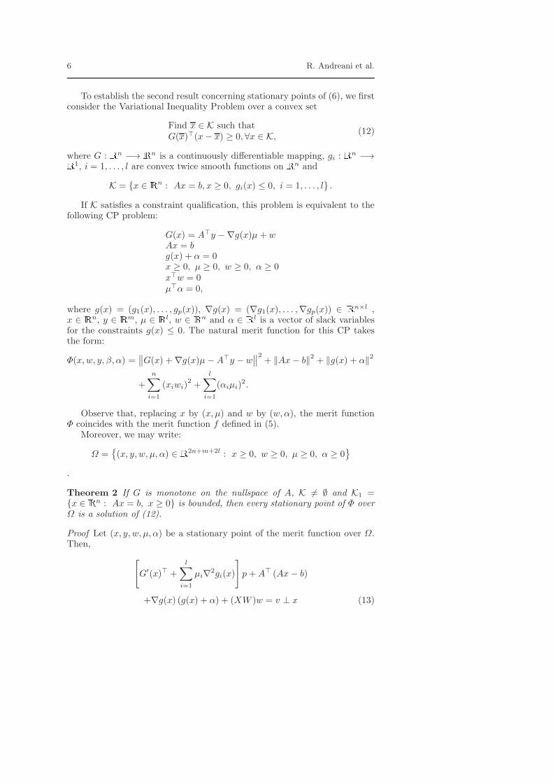
To establish the second result concerning stationary points of (6), we firstconsider the Variational Inequality Problem over a convex set

Find x ∈ K such thatG(x)⊤(x− x) ≥ 0, ∀x ∈ K,

(12)

where G : Rn −→ Rn is a continuously differentiable mapping, gi : Rn −→R1, i = 1, . . . , l are convex twice smooth functions on Rn and

K = x ∈ Rn : Ax = b, x ≥ 0, gi(x) ≤ 0, i = 1, . . . , l .

If K satisfies a constraint qualification, this problem is equivalent to thefollowing CP problem:

G(x) = A⊤y −∇g(x)µ+ wAx = bg(x) + α = 0x ≥ 0, µ ≥ 0, w ≥ 0, α ≥ 0x⊤w = 0µ⊤α = 0,

where g(x) = (g1(x), . . . , gp(x)), ∇g(x) = (∇g1(x), . . . ,∇gp(x)) ∈ Rn×l ,x ∈ Rn, y ∈ Rm, µ ∈ Rl, w ∈ Rn and α ∈ Rl is a vector of slack variablesfor the constraints g(x) ≤ 0. The natural merit function for this CP takesthe form:

Φ(x,w, y, β, α) =∥∥G(x) +∇g(x)µ −A⊤y − w

∥∥2 + ‖Ax− b‖2 + ‖g(x) + α‖2

+

n∑

i=1

(xiwi)2+

l∑

i=1

(αiµi)2.

Observe that, replacing x by (x, µ) and w by (w,α), the merit functionΦ coincides with the merit function f defined in (5).

Moreover, we may write:

Ω =(x, y, w, µ, α) ∈ R2n+m+2l : x ≥ 0, w ≥ 0, µ ≥ 0, α ≥ 0

.

Theorem 2 If G is monotone on the nullspace of A, K 6= ∅ and K1 =x ∈ Rn : Ax = b, x ≥ 0 is bounded, then every stationary point of Φ overΩ is a solution of (12).

Proof Let (x, y, w, µ, α) be a stationary point of the merit function over Ω.Then,

[G′(x)⊤ +

l∑

i=1

µi∇2gi(x)

]p+A⊤ (Ax− b)

+∇g(x) (g(x) + α) + (XW )w = v ⊥ x (13)

Merit function for complementarity 7

−Ap = 0 (14)

−p+ (XW )x = z ⊥ w (15)

(g(x) + α) + (ΛΥ )µ = β ⊥ α (16)

∇g(x)⊤p+ (ΛΥ )α = γ ⊥ µ (17)

x, v, z, w, α, β, γ, µ ≥ 0,

where ∇2gi(x) is the Hessian of gi at x, Λ = diag(αi) ∈ Rl×l, Υ = diag(µi) ∈Rl×l and X = diag(xi) ∈ Rn×n, W = diag(wi) ∈ Rn×n, and

p = G(x) +∇g(x)µ−A⊤y − w.

By (16) and (17),

p⊤∇g(x) (g(x) + α) = [γ − (ΛΥ )α]⊤[β − ΛΥ )µ]

= γ⊤β +

l∑

i=1

(αiµi)3.

Furthermore, using (13) and (15), we have that

p⊤(XW )w = −z⊤(XW )w + x⊤(XWXW )w

=

n∑

i=1

ziw2i xi +

n∑

i=1

x3iw

3i

=

n∑

i=1

(xiwi)3,

and, by (14),

p⊤v = v⊤(XW )x− z⊤v =

n∑

i=1

x2iwivi − z⊤v = −z⊤v.

Since Ap = 0, then p = Zd, for some d ∈ Rn−m, where Z ∈ Rn×(n−m)

is a matrix whose columns form a basis of the nullspace of A. The aboveinequalities and (14) yield:

d⊤Z⊤

[G′(x)⊤ +

l∑

i=1

µi∇2gi(x)

]Zd =

−

(v⊤z + γ⊤β +

l∑

i=1

(αiµi)3 +

n∑

i=1

(xiwi)3

)≤ 0.

Since Z⊤

[G′(x)⊤ +

l∑

i=1

µi∇2gi(x)

]Z is positive semi–definite, it follows that

d⊤Z⊤

[G′(x)⊤ +

l∑

i=1

µi∇2gi(x)

]Zd = 0

8 R. Andreani et al.

and

v⊤z = 0β⊤γ = 0α⊤µ = 0x⊤w = 0.

Since (XW )x = 0, it follows from (15) that

p = −z ≤ 0.

Hence,

Ap = 0, p ≤ 0.

Since K1 = x ∈ Rn : Ax = b, x ≥ 0 is bounded, then p = 0. Therefore,using x⊤w = α⊤µ = 0 in the equations (13) – (17), we obtain:

A⊤(Ax − b) +∇g(x)(g(x) + α) = vg(x) + α = β

x ≥ 0, v ≥ 0, α ≥ 0, β ≥ 0x⊤v = α⊤β = 0.

(18)

Define:

I = i ∈ 1, 2, . . . ,m : gi(x) ≥ 0 .

If i /∈ I, we have that gi(x) < 0, so, by (18), αi ≥ βi. Thus, since αiβi = 0,we obtain that βi = 0. Therefore, gi(x) + αi = 0.

If i ∈ I we have that gi(x) + αi = βi > 0. Thus, since αiβi = 0, we havethat αi = 0. Therefore, the first equation of (18) may be written:

A⊤(Ax − b) +∑

i∈I

∇gi(x)gi(x) = v. (19)

Since K 6= ∅, there exists x such that Ax = b, x ≥ 0. Pre-multiplying (19)by (x− x)⊤, we obtain:

(x− x)⊤[A⊤(Ax − b) +∑

i∈I

∇gi(x)gi(x)] = (x− x)⊤v.

Then, since x⊤v = 0,

‖Ax− b‖2 +∑

i∈I

∇gi(x)gi(x)] = −x⊤v ≤ 0. (20)

By the convexity of gi, we have:

gi(x)− gi(x) ≤ ∇gi(x)⊤(x− x), i = 1, . . . , p. (21)

By (20) and (21), using that gi(x) ≥ 0 for i ∈ I, we get:

‖Ax− b‖2 +∑

i∈I

gi(x)(gi(x)− gi(x) ≤ 0.

Merit function for complementarity 9

Since x is feasible, this implies that:

‖Ax− b‖2 +∑

i∈I

gi(x)2 ≤ 0.

Therefore, Ax = b and gi(x) = 0 for all i ∈ I. This completes the proof.

Remark. Equivalence results based on Fischer-Burmeister reformulationsusually do not need the compactness of the polytope K1. Compactification

of the domain may be obtained adding the equality∑n+1

i=1 xi = M for largeM , a transformation that does not alter the structure of problem (12). In [4]the conditions under which this type of transformation preserve the correctsolutions of the problem have been analyzed.

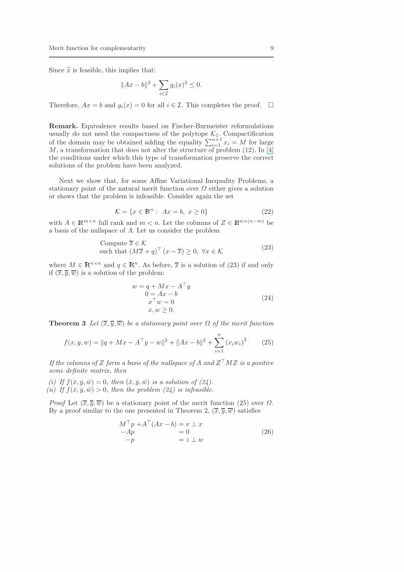
Next we show that, for some Affine Variational Inequality Problems, astationary point of the natural merit function over Ω either gives a solutionor shows that the problem is infeasible. Consider again the set

K = x ∈ Rn : Ax = b, x ≥ 0 (22)

with A ∈ Rm×n full rank and m < n. Let the columns of Z ∈ Rn×(n−m) bea basis of the nullspace of A. Let us consider the problem

Compute x ∈ Ksuch that (Mx+ q)⊤ (x− x) ≥ 0, ∀x ∈ K

(23)

where M ∈ Rn×n and q ∈ Rn. As before, x is a solution of (23) if and onlyif (x, y, w) is a solution of the problem:

w = q +Mx−A⊤y0 = Ax− bx⊤w = 0x,w ≥ 0.

(24)

Theorem 3 Let (x, y, w) be a stationary point over Ω of the merit function

f(x, y, w) = ‖q +Mx−A⊤y − w‖2 + ‖Ax− b‖2 +n∑

i=1

(xiwi)2

(25)

If the columns of Z form a basis of the nullspace of A and Z⊤MZ is a positivesemi–definite matrix, then

(i) If f(x, y, w) = 0, then (x, y, w) is a solution of (24).(ii) If f(x, y, w) > 0, then the problem (24) is infeasible.

Proof Let (x, y, w) be a stationary point of the merit function (25) over Ω.By a proof similar to the one presented in Theorem 2, (x, y, w) satisfies

M⊤p +A⊤(Ax− b) = v ⊥ x−Ap = 0−p = z ⊥ w

(26)

10 R. Andreani et al.

x ⊥ w, x, v, z, w ≥ 0,

wherep = q +Mx−A⊤y − w.

These are the KKT conditions of the following convex quadratic program

minx,y,w

‖q +Mx−A⊤y − w‖2 + ‖Ax− b‖2

subject to x ≥ 0, w ≥ 0.

The result follows since the objective function is convex.

Let us now consider a Quadratic Program (QP):

Minimize q⊤x+ 12x

⊤Mx = f(x)subject to Ax = b

x ≥ 0.(27)

The KKT conditions for this Program consist of an LCP of the form of (24).By Theorem 3, if f is convex over the nullspace of A, then a stationary point(x, y, w) of the merit function (25) over Ω solves the convex QP, in the sensethat:

1. If f(x, y, w) = 0, then x is a global minimum of the quadratic program;2. If f(x, y, w) > 0, then the quadratic program is primal or dual infeasible.

In particular, this result applies to Linear Programming problems, whichhave the form (27) with M = 0.

3 Conclusions

In this paper we considered the Complementarity Problem CP in the form(4), as a general square nonlinear system that includes complementarity con-straints. This form is more general than the ones that represent optimalityconditions and variational inequality problems. We used the natural squarednorm of the residual as merit function, and we showed that stationary pointsof this function over Ω are solutions of the problem or possess singular Ja-cobians (Theorem 1). Furthermore, for the variational inequality problem(VI) with a mapping F and a convex domain K, under a weak monotonicityassumption and a boundedness condition on K, stationary points are solu-tions of the problem (Theorem 2). When F is affine and K is a polyhedron,a stationary point of the natural merit function either gives a solution tothe VI or shows that the VI has no solution (Theorem 3). In particular, forlinear and convex quadratic programs, a stationary point of the associatednatural merit function either provides an optimal solution or establishes thatthe problem is primal or dual infeasible.

Nonlinear systems of equations with bounds on the variables have beenconsidered in [5]. Many other papers (see, por example, [6–8]) deal withconvex-constrained optimization and are able to handle large scale problems.

Merit function for complementarity 11

The results presented here help to predict what can be expected from thosegeneral convex-constraint approaches, when applied to the complementarityproblem using the natural sum-of-squares merit function. Moreover, the em-ployment of simply-constrained instead of unconstrained reformulations isadvantageous to avoid possible convergence to stationary points that do notsatisfy positivity constraints and do not fulfill the monotonicity-like assump-tions required for equivalence results.

Interior point methods applied to specific complementarity problems weredefined in [24,27,31,32,34,36], among others. The effect of degeneracy wasanalyzed in [10,26]. A large number of numerical experiments using a methodthat combines interior points and projected gradients was given in [30].

In spite of the large number of specific methods for different complemen-tarity problems, many users prefer to use well established bound-constraintminimization algorithms for solving practical problems. Since these solversusually generate sequences that converge to first-order stationary points, therelations between stationary points and solutions will continue to be algo-rithmically relevant.

Acknowledgements The authors are indebted to the Associate Editor and twoanonymous referees for their insightful comments on this paper.

References

1. R. Andreani, E. G. Birgin, J. M. Martınez, and M. L. Schuverdt, AugmentedLagrangian methods under the Constant Positive Linear Dependence con-straint qualification. Mathematical Programming 111 (2008), pp. 5-32 (2008).

2. R. Andreani, A. Friedlander, J. M. Martınez. On the solution of finite-dimensional variational inequalities using smooth optimization with simplebounds. Journal on Optimization Theory and Applications 94 (1997) pp. 635-657.

3. R. Andreani, A. Friedlander, and S. A. Santos, On the resolution of the gen-eralized nonlinear complementarity problem. SIAM Journal on Optimization12 (2001), pp. 303-321.

4. R. Andreani and J. M. Martınez, Reformulation of variational inequalities ona simplex and compactification of complementarity problems. SIAM Journalon Optimization 10 (2000), pp. 878-895.

5. S. Bellavia and B. Morini,An interior global method for nonlinear systemswith simple bounds. Optimization Methods and Software 20 (2005), pp. 1-22.

6. E.G. Birgin, J.M. Martınez and M. Raydan, Nonmonotone spectral projectedgradient methods on convex sets. SIAM Journal on Optimization, 10 (2000),pp. 1196-1211.

7. E.G. Birgin, J.M. Martınez and M. Raydan, Algorithm 813 SPG: Software forconvex-constrained optimization. ACM Transactions on Mathematical Soft-ware, 27 (2001), pp. 340-349.

8. E.G. Birgin, J.M. Martınez and M. Raydan, Inexact spectral projected gradientmethods on convex sets. IMA Journal of Numerical Analysis, 23 (2003), pp.340-349.

9. R. Cottle, J. S. Pang and H. Stone, The linear complementarity problem.Academic Press, New York, 1992.

10. H. Dan, N. Yamashita and M. Fukushima, A superlinearly convergent algo-rithm for the monotone nonlinear complementarity problem without unique-ness and nondegeneracy conditions. Mathematics of Operations Research, 27(2002), pp. 743-753.

12 R. Andreani et al.

11. F. Facchinei, A. Fischer and C. Kanzow, A semismooth Newton method forvariational inequalities: The case of box constraints. In M. C. Ferris and J.-S.Pang (eds.): Complementarity and Variational Problems - State of the Art,SIAM, Philadelphia 1997, 76-90.

12. F. Facchinei, A. Fischer and C. Kanzow, Regularity properties of a semismoothreformulation of variational inequalities. SIAM Journal on Optimization, 8(1998), pp. 850-869.

13. F. Facchinei, A. Fischer, C. Kanzow and J-M Peng, A simply constrained opti-mization reformulation of KKT systems arising from variational inequalities.Applied Mathematics and Optimization, 40 (1999), pp. 19–37.

14. F. Facchinei and J. S. Pang, Finite-Dimensional inequalities and complemen-tarity problems. Springer, New York, 2003.

15. F. Facchinei and J. Soares, A new merit function for complementarity prob-lems and a related algorithm. SIAM Journal on Optimization, 7 (1997), pp.225-247.

16. L. Fernandes, A. Friedlander, M. C. Guedes and J. Judice, Solution of a gen-eral linear complementarity problem using smooth optimization and its appli-cations to bilinear programming and LCP. Applied Mathematics and Opti-mization, 43 (2001), pp. 1-19.

17. L. Fernandes, J. Judice and I. Figueiredo, On the solution of a finite ele-ment approximation of a linear obstacle plate problem. International Journalof Applied Mathematics and Computer Science, 12(2002), pp. 27-40.

18. M. C. Ferris, C. Kanzow and T. S. Munson, Feasible Descent Algorithms forMixed Complementarity Problems. Mathematical Programming 86 (1999), pp.475–497.

19. A. Fischer, New constrained optimization reformulation of complementarityproblems. Journal of Optimization Theory and Applications 12 (2001), pp.303-321.

20. A. Friedlander, J. M. Martınez and S. A. Santos, Solution of linear comple-mentarity problems using minimization with simple bounds. Journal of GlobalOptimization 6 (1995), pp. 1-15.

21. A. Friedlander, J. M. Martınez and S. A. Santos, A new strategy for solvingvariational inequalities on bounded polytopes. Numerical Functional Analysisand Optimization 16 (1995), pp. 653-668.

22. J. Haslinger, I. Hlavacek and J. Necas, Numerical methods for unilateral prob-lems in solid mechanics. In Handbook of Numerical Analysis, P. Ciarlet andJ. L. Lions, eds., vol. IV, North-Holland, Amsterdam, 1999.

23. N. Kikuchi and J. T. Oden, Contact Problems in Elasticity: a Study of Vari-ational Inequalities and Finite Elements. SIAM, Philadelphia, 1988.

24. M. Kojima, N. Megiddo, T. Noma and A. Yoshise, A Unified Approachto Interior-Point Algorithms for Linear Complementarity Problems. LectureNotes in Computer Science 538, Springer-Verlag, Berlin, 1991.

25. O. L. Mangasarian and M. Solodov, Nonlinear complementarity as un-constrained and constrained minimization. Mathematical Programming, 62(1993), pp. 277–297.

26. R. D. C. Monteiro and S. J. Wright, Local convergence of interior-point algo-rithms for degenerate monotone LCP problems. Computational Optimizationand Applications, 3 (1994), pp. 131-155.

27. R. D. C. Monteiro and S. J. Wright, Superlinear primal-dual affine scalingalgorithms for LCP. Mathematical Programming, 69 (1995), pp. 311-333.

28. J. J. More, Global methods for nonlinear complementarity problems. Mathe-matics of Operations Research 21 (1996), pp. 598-614.

29. K. Murty, Linear complementarity, linear and nonlinear programming. Hel-dermann Verlag, Berlin, 1988.

30. J. Patrıcio, Algoritmos de Pontos Interiores para Problemas ComplementaresMonotonos e suas Aplicacoes (in Portuguese), PhD Thesis, University ofCoimbra, Portugal, 2007.

31. F. Potra, Primal-Dual affine scaling interior point methods for linear comple-mentarity problems. SIAM Journal on Optimization, 19 (2008), pp. 114–143.

Merit function for complementarity 13

32. D. Ralph and S. Wright, Superlinear convergence of an interior-point methodfor monotone variational inequalities. In Complementarity and VariationalProblems. State of Art, Edited by M. C. Ferris and J-S Pang, SIAM Publica-tions, 1998.

33. A. Shapiro,Sensitivity analysis of parameterized variational inequalities.Mathematics of Operations Research 30 (2005), pp. 109-126.

34. E. Simantiraki and D. Shanno, An infeasible interior point method for linearcomplementarity problem. SIAM Journal on Optimization 7 (1997), pp. 620-640.

35. M. V. Solodov,Stationary points of bound constrained minimization reformu-lations. Journal of Optimization Theory and Applications 94 (1997) pp. 449-467.

36. S. J. Wright and D. Ralph, A superlinear infeasible interior-point algorithmsfor monotone complementarity problems. Mathematics of Operations Re-search, 21 (1996), pp. 815-838.