THE MATRIX APPLICATION TO LINEAR PROGRAMMING PROBLEM (A BASIC FACT IN MATHS) By Victor E. A. Iteye
25
THE MATRIX APPLICATION TO LINEAR PROGRAMMING PROBLEM (A BASIC FACT IN MATHS) By Victor E. A. Iteye The Matrix Application using the Simplex Method The simplex method is a mathematical technique and is a general algebraic method for solving any linear programming model. In this section, we are going to show its matrix application. A linear programming problem involving more than two variables can be solved by algebraic method. This algebraic method is known as simplex method. This method consists of a number of steps. In the first step, we get the value of z which is equal to the value at one vertex by the graphical solution. In the next step the value of Z will be better than the previous one and is equal to the next adjoining vertex and so on. Since, the number of vertices is finite; the simple method also consists of finite number of steps to get the optimal solution. In the first step, we ensure that each constraint is written with a positive right – hand side constant term. Then we express all inequalities as equations by the introduction of slack variables For example, − ݔ+2 ݕ≤ 6 can be written as – ݔ+2 ݕ+ ݓ1=6 5 ݔ+ 4 ݕ≤ 40 can be written as 5 ݔ+4 ݕ+ ݓଵ = 40, where ݓଵ ݓଶ are positive (or Zero) variables with unit coefficient required to make up the left –hand side to the value of the right –hand side constant term. The new variables ݓଵ ݓଶ ݎ ݏ ݒݎ ݏComputation of the Simplex
Transcript of THE MATRIX APPLICATION TO LINEAR PROGRAMMING PROBLEM (A BASIC FACT IN MATHS) By Victor E. A. Iteye

THE MATRIX APPLICATION TO LINEAR PROGRAMMING PROBLEM (A BASIC FACT IN MATHS) By Victor E. A. Iteye
The Matrix Application using the Simplex Method
The simplex method is a mathematical technique and is a general algebraic
method for solving any linear programming model. In this section, we are going to
show its matrix application. A linear programming problem involving more than two
variables can be solved by algebraic method. This algebraic method is known as
simplex method.
This method consists of a number of steps. In the first step, we get the value of
z which is equal to the value at one vertex by the graphical solution. In the next step
the value of Z will be better than the previous one and is equal to the next adjoining
vertex and so on. Since, the number of vertices is finite; the simple method also
consists of finite number of steps to get the optimal solution.
In the first step, we ensure that each constraint is written with a positive right –
hand side constant term. Then we express all inequalities as equations by the
introduction of slack variables
For example, −푥 + 2푦 ≤ 6 can be written as – 푥 + 2푦 + 푤1 = 6푎푛푑5푥 +
4푦 ≤ 40 can be written as 5푥 + 4푦 + 푤 = 40, where 푤 푎푛푑푤 are positive (or
Zero) variables with unit coefficient required to make up the left –hand side to the
value of the right –hand side constant term. The new variables
푤 푎푛푑푤 푎푟푒푐푎푙푙푒푑푠푙푎푐푘푣푎푟푖푎푏푙푒푠
Computation of the Simplex
THE MATRIX APPLICATION TO LINEAR PROGRAMMING PROBLEM (A BASIC FACT IN MATHS) By Victor E. A. Iteye
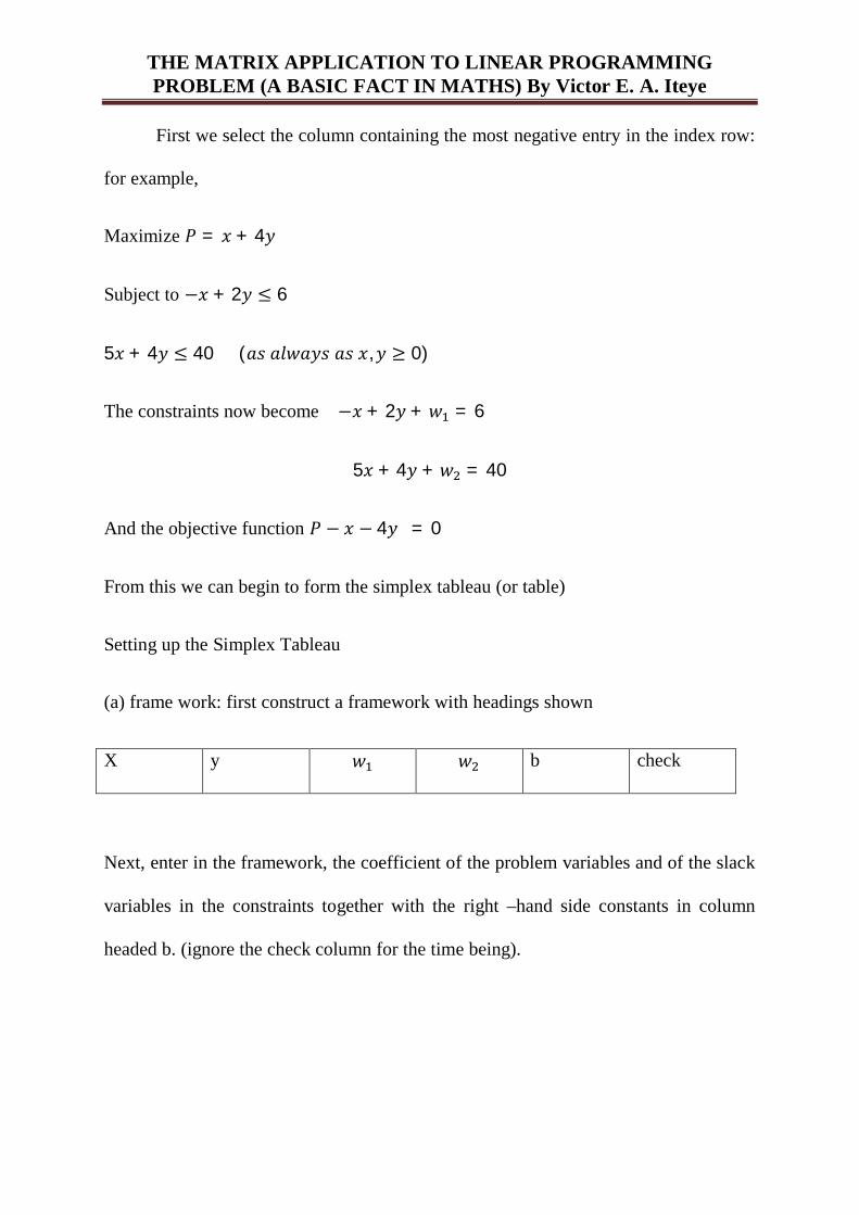
First we select the column containing the most negative entry in the index row:
for example,
Maximize 푃 = 푥 + 4푦
Subject to −푥 + 2푦 ≤ 6
5푥 + 4푦 ≤ 40(푎푠푎푙푤푎푦푠푎푠푥,푦 ≥ 0)
The constraints now become −푥 + 2푦 + 푤 = 6
5푥 + 4푦 + 푤 = 40
And the objective function 푃 − 푥 − 4푦 = 0
From this we can begin to form the simplex tableau (or table)
Setting up the Simplex Tableau
(a) frame work: first construct a framework with headings shown
X y 푤 푤 b check
Next, enter in the framework, the coefficient of the problem variables and of the slack
variables in the constraints together with the right –hand side constants in column
headed b. (ignore the check column for the time being).
THE MATRIX APPLICATION TO LINEAR PROGRAMMING PROBLEM (A BASIC FACT IN MATHS) By Victor E. A. Iteye
body Unit matrix
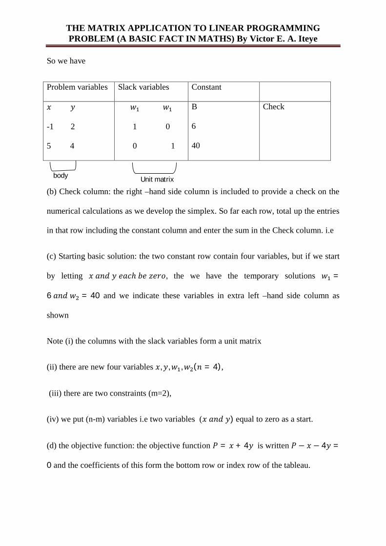
So we have
Problem variables Slack variables Constant
푥 푦
-1 2
5 4
푤 푤
1 0
0 1
B
6
40
Check
(b) Check column: the right –hand side column is included to provide a check on the
numerical calculations as we develop the simplex. So far each row, total up the entries
in that row including the constant column and enter the sum in the Check column. i.e
(c) Starting basic solution: the two constant row contain four variables, but if we start
by letting 푥푎푛푑푦푒푎푐ℎ푏푒푧푒푟표, the we have the temporary solutions 푤 =
6푎푛푑푤 = 40 and we indicate these variables in extra left –hand side column as
shown
Note (i) the columns with the slack variables form a unit matrix
(ii) there are new four variables 푥,푦,푤 ,푤 (푛 = 4),
(iii) there are two constraints (m=2),
(iv) we put (n-m) variables i.e two variables (푥푎푛푑푦) equal to zero as a start.
(d) the objective function: the objective function 푃 = 푥 + 4푦 is written 푃 − 푥 − 4푦 =
0 and the coefficients of this form the bottom row or index row of the tableau.
THE MATRIX APPLICATION TO LINEAR PROGRAMMING PROBLEM (A BASIC FACT IN MATHS) By Victor E. A. Iteye
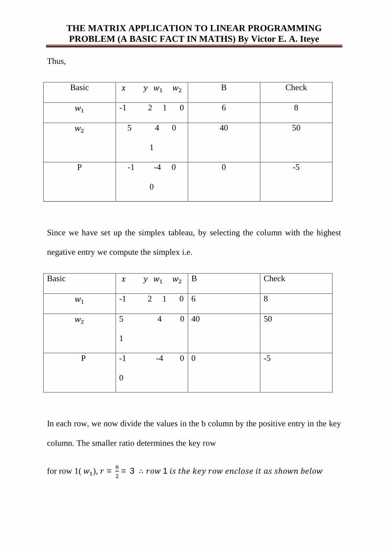
Thus,
Basic 푥푦푤 푤 B Check
푤 -1 2 1 0 6 8
푤 5 4 0
1
40 50
P -1 -4 0
0
0 -5
Since we have set up the simplex tableau, by selecting the column with the highest
negative entry we compute the simplex i.e.
Basic 푥푦푤 푤 B Check
푤 -1 2 1 0 6 8
푤 5 4 0
1
40 50
P -1 -4 0
0
0 -5
In each row, we now divide the values in the b column by the positive entry in the key
column. The smaller ratio determines the key row
for row 1( 푤 ), 푟 = = 3 ∴ 푟표푤1푖푠푡ℎ푒푘푒푦푟표푤푒푛푐푙표푠푒푖푡푎푠푠ℎ표푤푛푏푒푙표푤
THE MATRIX APPLICATION TO LINEAR PROGRAMMING PROBLEM (A BASIC FACT IN MATHS) By Victor E. A. Iteye
Key row
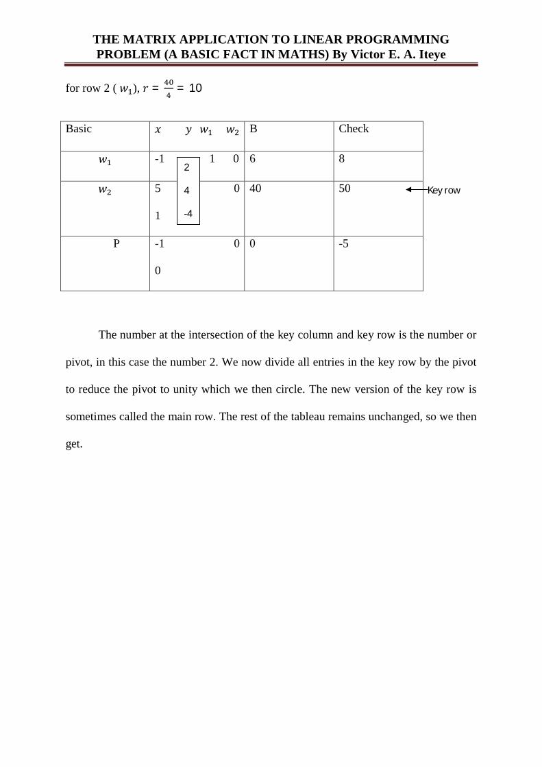
for row 2 ( 푤 ), 푟 = = 10
Basic 푥푦푤 푤 B Check
푤 -1 1 0 6 8
푤 5 0
1
40 50
P -1 0
0
0 -5
The number at the intersection of the key column and key row is the number or
pivot, in this case the number 2. We now divide all entries in the key row by the pivot
to reduce the pivot to unity which we then circle. The new version of the key row is
sometimes called the main row. The rest of the tableau remains unchanged, so we then
get.
2
4
-4
THE MATRIX APPLICATION TO LINEAR PROGRAMMING PROBLEM (A BASIC FACT IN MATHS) By Victor E. A. Iteye
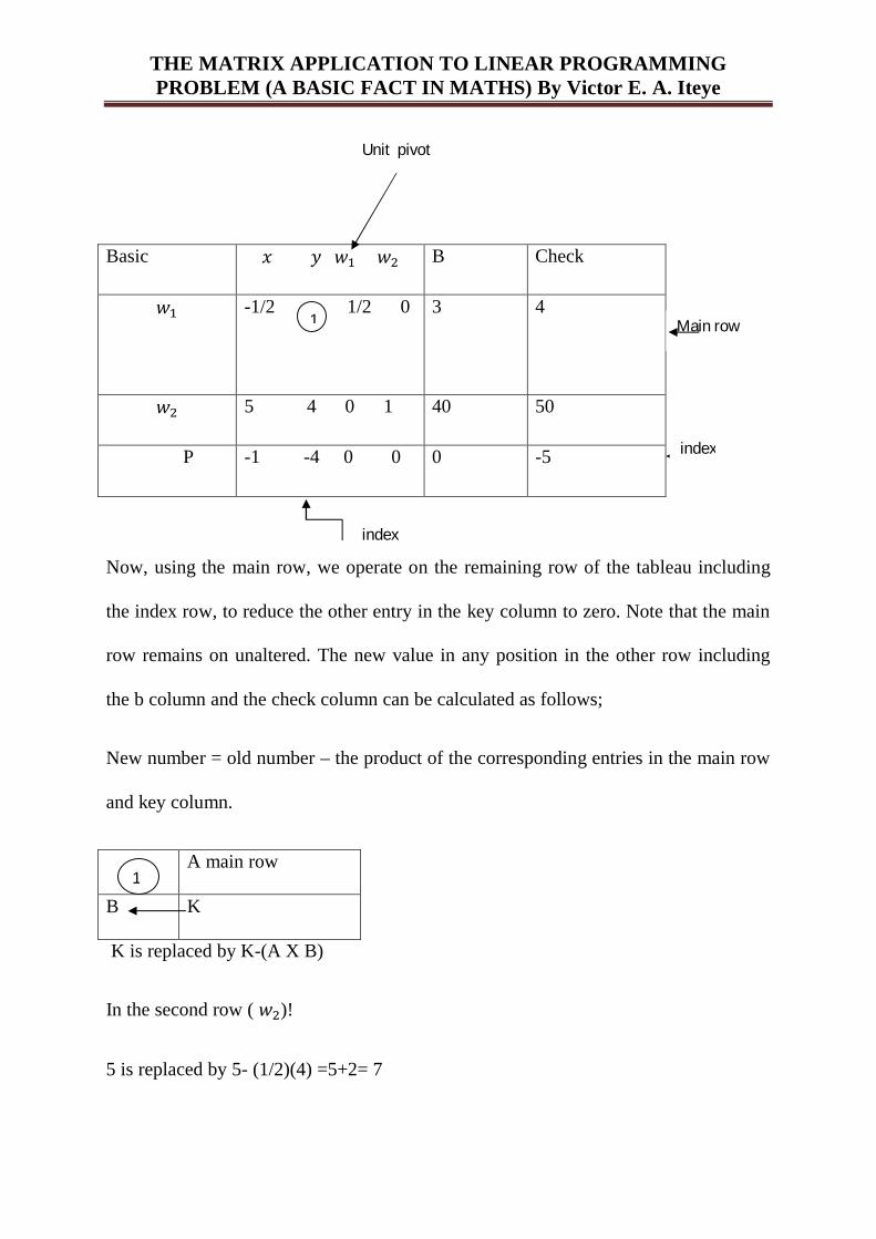
Basic 푥푦푤 푤 B Check
푤 -1/2 1/2 0 3 4
푤 5 4 0 1 40 50
P -1 -4 0 0 0 -5
Now, using the main row, we operate on the remaining row of the tableau including
the index row, to reduce the other entry in the key column to zero. Note that the main
row remains on unaltered. The new value in any position in the other row including
the b column and the check column can be calculated as follows;
New number = old number – the product of the corresponding entries in the main row
and key column.
A main row
B K
K is replaced by K-(A X B)
In the second row ( 푤 )!
5 is replaced by 5- (1/2)(4) =5+2= 7
1
Unit pivot
Main row
index
index
1

THE MATRIX APPLICATION TO LINEAR PROGRAMMING PROBLEM (A BASIC FACT IN MATHS) By Victor E. A. Iteye
4 is replace by 4- (1)(4) = 4-4 =0
0 is replaced by 0- (1/2) (4) =0 -2 = -2
1 is replaced by 1- 0 (4) =1-0 =1
40 is replaced by 40 – (3)(4) =40 -12 =28
50 is replaced by 50 –(4)(4) = 50 -16 =34
And in the third row (p):
-1 is replaced by – 1 -(-1/2)(-4) =- 1 -3 = -3
Completing the operations for rows ( 푤 )푎푛푑(푝), we have
Basic 푥푦푤 푤 B Check
푤 -1/2 1 1/2 0 3 4
푤 7 4 0 1 28 34
P -1 -4 0 0 12 11
The Dual Simplex Algorithm
(i) While in the optimal tableau, select the leaving basic variable which will be the
one with most negative right hand side.
(ii) for the entry variables, determinant the
푚푖푛푧 − 푐푎
=푧 − 푐푎

THE MATRIX APPLICATION TO LINEAR PROGRAMMING PROBLEM (A BASIC FACT IN MATHS) By Victor E. A. Iteye
Where Z-C is the objective role moment headed by 푢 (푒푛푡푟푦푣푎푟푖푎푏푙푒)
(iii) determine the solution using the Gauss – Jordan elimination method.
(iv) stop where there is no negative right hand side, if otherwise go to step (1)
Example
Solve the linear programming problem below using the Dual simplex method.
min푍 = 6푢 + 5푢
Subject to
푈 + 4푈 + 5푈 ≥ 12
7푈 + 5푈 ≥ 35
푈 ,푈 ≥ 0
Solution
In dual simplex method a linear constant having surplus variables are multiplied
by – 1. hence, the program becomes
min푍 = 6푢 + 5푢 + 0푢 + 0푈
Subject to
−푈 −4푈 + 푈 = −12−7푈 −5푈 + 푈 = −35푈 푈 , 푈 ≥ 0
Next, we solve using a tableau.
THE MATRIX APPLICATION TO LINEAR PROGRAMMING PROBLEM (A BASIC FACT IN MATHS) By Victor E. A. Iteye
Tableau 1
BV 푈 푈 푈 푈 RHS
푈 -1 -4 0 푈 -12
푈 - 7 - 5 0 1 - 35
Z 6 5 0 0
The arrow at 푈 has the most negative RHS and hence the leaving variables.
Computing for the entry variables by the algorithm (II); we have
−67
−55
will give the smallest quotient hence -7 is the pivot element and 푈 the entry
variable.
Tableau II
BV 푈 푈 푈 푈 RHS
푈 0 -23/7 1 -1/7 -7
푈 1 5/7 0 1/7 5
Z 6 5/7 0 6/7 -30
By Gauss- Jordan computation, we have
//
//
= 1푎푛푑 × =
We have 1 and 6 which implies that 푈 is the entry variable.
THE MATRIX APPLICATION TO LINEAR PROGRAMMING PROBLEM (A BASIC FACT IN MATHS) By Victor E. A. Iteye
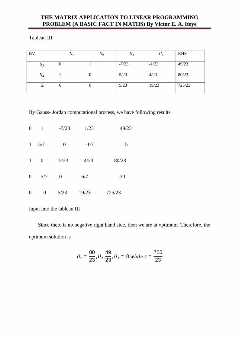
Tableau III
BV 푈 푈 푈 푈 RHS
푈 0 1 -7/23 -1/23 49/23
푈 1 0 5/23 4/23 80/23
Z 6 0 5/23 19/23 725/23
By Gauss- Jordan computational process, we have following results
0 1 -7/23 1/23 49/23
1 5/7 0 -1/7 5
1 0 5/23 4/23 80/23
0 5/7 0 6/7 -30
0 0 5/23 19/23 725/23
Input into the tableau III
Since there is no negative right hand side, then we are at optimum. Therefore, the
optimum solution is
푈 =8023
,푈 ,4923
,푈 = 0푤ℎ푖푙푒푧 =72523
THE MATRIX APPLICATION TO LINEAR PROGRAMMING PROBLEM (A BASIC FACT IN MATHS) By Victor E. A. Iteye
Solution of integer programming problems:
Integer programming ideas, with problems of minimizing and maximizing a
function of many variables subject to equality and inequality constraints and
integrality restrictions on some or all of the variables
Types of integer programming problems
(1) pure (all integer) programming
(2) mixed integer programming
(3) zero – one (binary) integer programming
For convenience and for the purpose of this work, we are concentrating on pure
integer –programming.
The pure integer –programming model is a linear programming model where all
the decision, variables are restricted to integer values which are non –negative.
However if only some of the variables are integers, the problem is a mixed integer
program.
THE MATRIX APPLICATION TO LINEAR PROGRAMMING PROBLEM (A BASIC FACT IN MATHS) By Victor E. A. Iteye
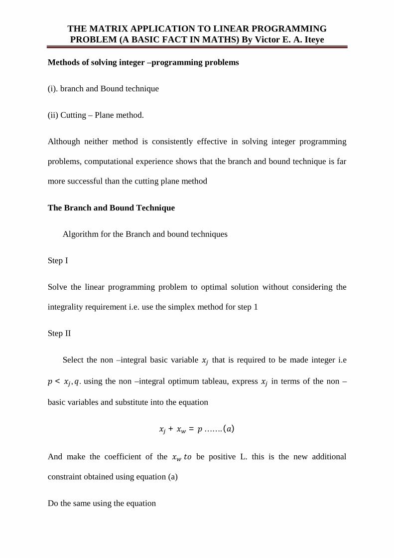
Methods of solving integer –programming problems
(i). branch and Bound technique
(ii) Cutting – Plane method.
Although neither method is consistently effective in solving integer programming
problems, computational experience shows that the branch and bound technique is far
more successful than the cutting plane method
The Branch and Bound Technique
Algorithm for the Branch and bound techniques
Step I
Solve the linear programming problem to optimal solution without considering the
integrality requirement i.e. use the simplex method for step 1
Step II
Select the non –integral basic variable 푥 that is required to be made integer i.e
푝 < 푥 , 푞. using the non –integral optimum tableau, express 푥 in terms of the non –
basic variables and substitute into the equation
푥 + 푥 = 푝… … . (푎)
And make the coefficient of the 푥 푡표 be positive L. this is the new additional
constraint obtained using equation (a)
Do the same using the equation
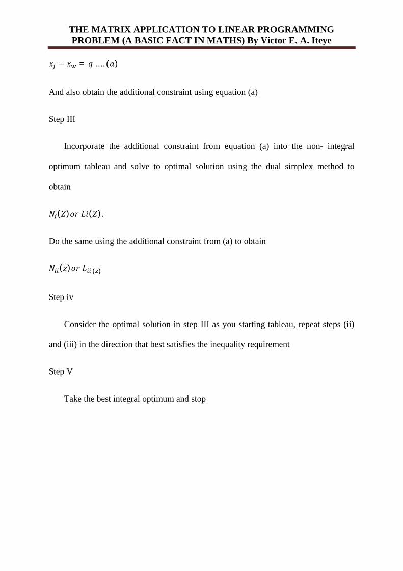
THE MATRIX APPLICATION TO LINEAR PROGRAMMING PROBLEM (A BASIC FACT IN MATHS) By Victor E. A. Iteye
푥 − 푥 = 푞… . (푎)
And also obtain the additional constraint using equation (a)
Step III
Incorporate the additional constraint from equation (a) into the non- integral
optimum tableau and solve to optimal solution using the dual simplex method to
obtain
푁 (푍)표푟퐿푖(푍).
Do the same using the additional constraint from (a) to obtain
푁 (푧)표푟퐿 ( )
Step iv
Consider the optimal solution in step III as you starting tableau, repeat steps (ii)
and (iii) in the direction that best satisfies the inequality requirement
Step V
Take the best integral optimum and stop
THE MATRIX APPLICATION TO LINEAR PROGRAMMING PROBLEM (A BASIC FACT IN MATHS) By Victor E. A. Iteye
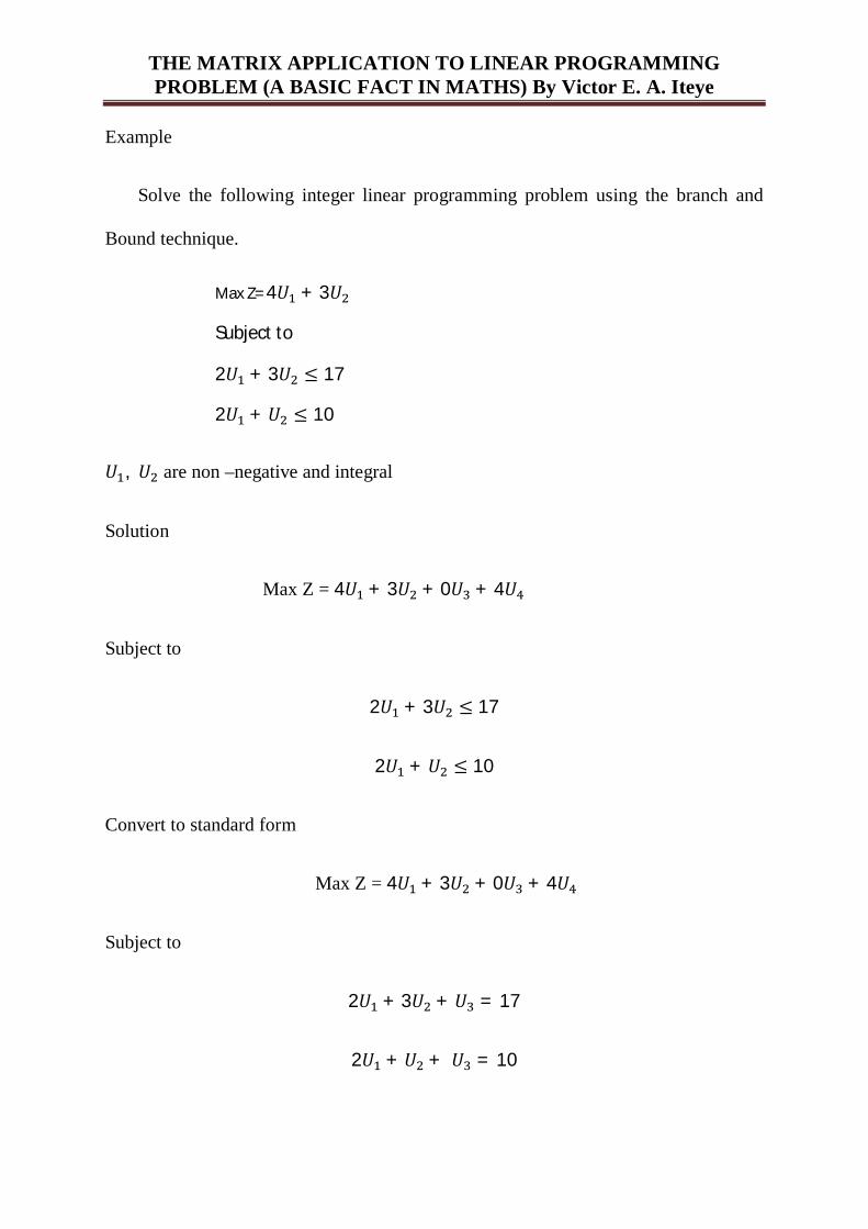
Example
Solve the following integer linear programming problem using the branch and
Bound technique.
푈 , 푈 are non –negative and integral
Solution
Max Z = 4푈 + 3푈 + 0푈 + 4푈
Subject to
2푈 + 3푈 ≤ 17
2푈 + 푈 ≤ 10
Convert to standard form
Max Z = 4푈 + 3푈 + 0푈 + 4푈
Subject to
2푈 + 3푈 + 푈 = 17
2푈 + 푈 + 푈 = 10
Max Z= 4푈 + 3푈
Subject to
2푈 + 3푈 ≤ 17
2푈 + 푈 ≤ 10
THE MATRIX APPLICATION TO LINEAR PROGRAMMING PROBLEM (A BASIC FACT IN MATHS) By Victor E. A. Iteye
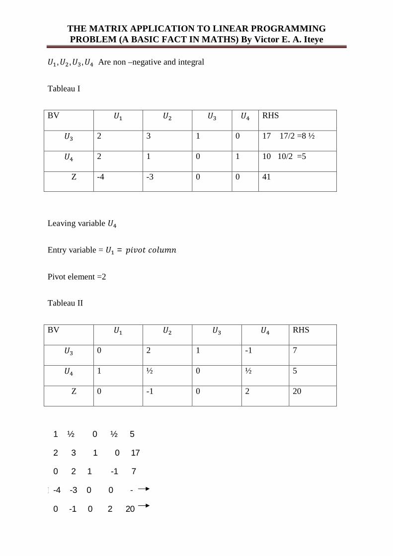
푈 ,푈 ,푈 ,푈 Are non –negative and integral
Tableau I
BV 푈 푈 푈 푈 RHS
푈 2 3 1 0 17 17/2 =8 ½
푈 2 1 0 1 10 10/2 =5
Z -4 -3 0 0 41
Leaving variable 푈
Entry variable = 푈 = 푝푖푣표푡푐표푙푢푚푛
Pivot element =2
Tableau II
BV 푈 푈 푈 푈 RHS
푈 0 2 1 -1 7
푈 1 ½ 0 ½ 5
Z 0 -1 0 2 20
Input into tableau II
1 ½ 0 ½ 5
2 3 1 0 17
0 2 1 -1 7
-4 -3 0 0 -
0 -1 0 2 20

THE MATRIX APPLICATION TO LINEAR PROGRAMMING PROBLEM (A BASIC FACT IN MATHS) By Victor E. A. Iteye
From tableau II (-1) is the most negative implies that 푈 is the entry variable while 푈
will give us the smallest quotient and hence the leaving variable next, go to
Tableau III
BV 푈 푈 푈 푈 RHS
푈 0 1 ½ -1/2 7/2
푈 1 0 ¼ ¾ 1/3/4
Z 0 0 1/2 3/2 47/2=23 ½
No=(23 ½ )
We make the pivot element to be unity and any other element above and below the
pivot element zero is
Input into tableau III above next,
푈 = 31/2푖. 푒3 < 푈 < 4 is the variable to be made integral
(i.e. 푈 ≤ 3,푈 ≥ 4 if 푈 ≤ 3, we add slack variable therefore,
푈 + 푈 = 3… (푎)
From tableau III
푈 + 푈 + 1/2푈 − 1/2푈 = 7/2
∴ 푈 = 7/2 − 푈 − 1/2푈 + 1/2푈
0 1 ½ -½ 7/2
1 ½ 0 ½ 5
1 0 -1/4 ¾ 13/4
0 -1 0 2 20
0 -1 1/2 3/2 47/2
THE MATRIX APPLICATION TO LINEAR PROGRAMMING PROBLEM (A BASIC FACT IN MATHS) By Victor E. A. Iteye
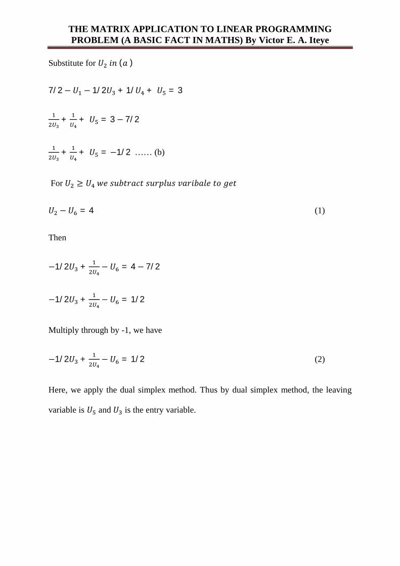
Substitute for 푈 푖푛(푎)
7/2 − 푈 − 1/2푈 + 1/푈 + 푈 = 3
+ + 푈 = 3 − 7/2
+ + 푈 = −1/2 …… (b)
For 푈 ≥ 푈 푤푒푠푢푏푡푟푎푐푡푠푢푟푝푙푢푠푣푎푟푖푏푎푙푒푡표푔푒푡
푈 − 푈 = 4 (1)
Then
−1/2푈 + − 푈 = 4 − 7/2
−1/2푈 + − 푈 = 1/2
Multiply through by -1, we have
−1/2푈 + − 푈 = 1/2 (2)
Here, we apply the dual simplex method. Thus by dual simplex method, the leaving
variable is 푈 and 푈 is the entry variable.

THE MATRIX APPLICATION TO LINEAR PROGRAMMING PROBLEM (A BASIC FACT IN MATHS) By Victor E. A. Iteye
Tableau IV
BV 푈 푈 푈 푈 푈 RHS
푈 0 1 0 0 1 3
푈 1 0 0 ½ -1/2 7/2
푈 0 0 1 -1 -2 1
Z 0 0 0 2 1 23 [푁 ( )]
0 0 1 -1 -2 1
0 1 1/2 -1/2 0 7/2
0 1 0 0 1 3
1 0 -1/4 3/4 0 13/2
1 0 0 1/2 -1/2 7/2
0 0 ½ 3/2 0 47/2
0 0 0 2 1 23
Input into tableau (1) above Ni fe(23) denoted a non –integral solution for tableau
with 23 as the objective function value

THE MATRIX APPLICATION TO LINEAR PROGRAMMING PROBLEM (A BASIC FACT IN MATHS) By Victor E. A. Iteye
Tableau V
BV 푈 푈 푈 푈 푈 RHS
푈 0 1 ½ ½ 0 7/2
푈 1 0 -1/4 ¾ 0 13/4
푈
1 0 0 ½ -1/2 -1/2
Z 0 0 0 2/7 0 47/2
Leaving variable =푈
Entry variable =푈
Again using the dual simplex method, we have the following computed table:
Tableau (VI)
BV 푈 푈 푈 푈 푈 RHS
푈 0 1 0 0 -1 7/2
푈 1 0 ½ 0 3/2 13/4
푈 0 0 -1 1 -1/2 -1/2
Z 0 0 0 2 3 22 [푁 ( )]

THE MATRIX APPLICATION TO LINEAR PROGRAMMING PROBLEM (A BASIC FACT IN MATHS) By Victor E. A. Iteye
0 0 -1 1 -2 1
0 1 1/2 -1/2 0 7/2
0 1 0 0 -1 4
1 0 -1/4 3/4 0 13/4
1 0 1/2 0 3/2 5/2
0 0 ½ 3/2 0 47/2
0 0 0 2 1 23
Input into tableau (i) above Nii (22) denoted a non –integral solution from tableau (ii)
with 22 as the objective function value i.e.
No (23 ½ )
Now, from tableau (i)
푈 = 7/2 = 31/2 ⇒ 3 < 푈 < 4
⇒ 푈 ≤ 3표푟푈 + 푈 = 3… . (4.3.5)
Tha is after adding a slack variable while
푈 ≥ 4표푟푈 − 푈 = 4 … ..(4.3.6)
Ni(23)
Ni(22)
THE MATRIX APPLICATION TO LINEAR PROGRAMMING PROBLEM (A BASIC FACT IN MATHS) By Victor E. A. Iteye
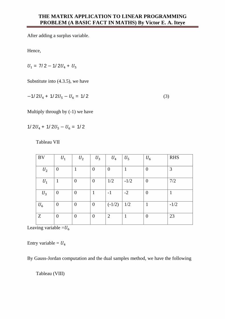
After adding a surplus variable.
Hence,
푈 = 7/2 − 1/2푈 + 푈
Substitute into (4.3.5), we have
−1/2푈 + 1/2푈 − 푈 = 1/2 (3)
Multiply through by (-1) we have
1/2푈 + 1/2푈 − 푈 = 1/2
Tableau VII
BV 푈 푈 푈 푈 푈 푈 RHS
푈 0 1 0 0 1 0 3
푈 1 0 0 1/2 -1/2 0 7/2
푈 0 0 1 -1 -2 0 1
푈 0 0 0 (-1/2) 1/2 1 -1/2
Z 0 0 0 2 1 0 23
Leaving variable =푈
Entry variable = 푈
By Gauss-Jordan computation and the dual samples method, we have the following
Tableau (VIII)
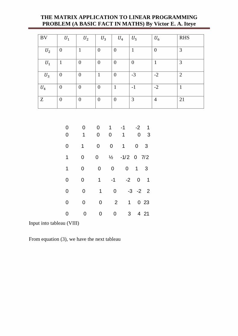
THE MATRIX APPLICATION TO LINEAR PROGRAMMING PROBLEM (A BASIC FACT IN MATHS) By Victor E. A. Iteye
BV 푈 푈 푈 푈 푈 푈 RHS
푈 0 1 0 0 1 0 3
푈 1 0 0 0 0 1 3
푈 0 0 1 0 -3 -2 2
푈 0 0 0 1 -1 -2 1
Z 0 0 0 0 3 4 21
Input into tableau (VIII)
From equation (3), we have the next tableau
0 0 0 1 -1 -2 1 0 1 0 0 1 0 3
0 1 0 0 1 0 3
1 0 0 ½ -1/2 0 7/2
1 0 0 0 0 1 3
0 0 1 -1 -2 0 1
0 0 1 0 -3 -2 2
0 0 0 2 1 0 23
0 0 0 0 3 4 21
THE MATRIX APPLICATION TO LINEAR PROGRAMMING PROBLEM (A BASIC FACT IN MATHS) By Victor E. A. Iteye
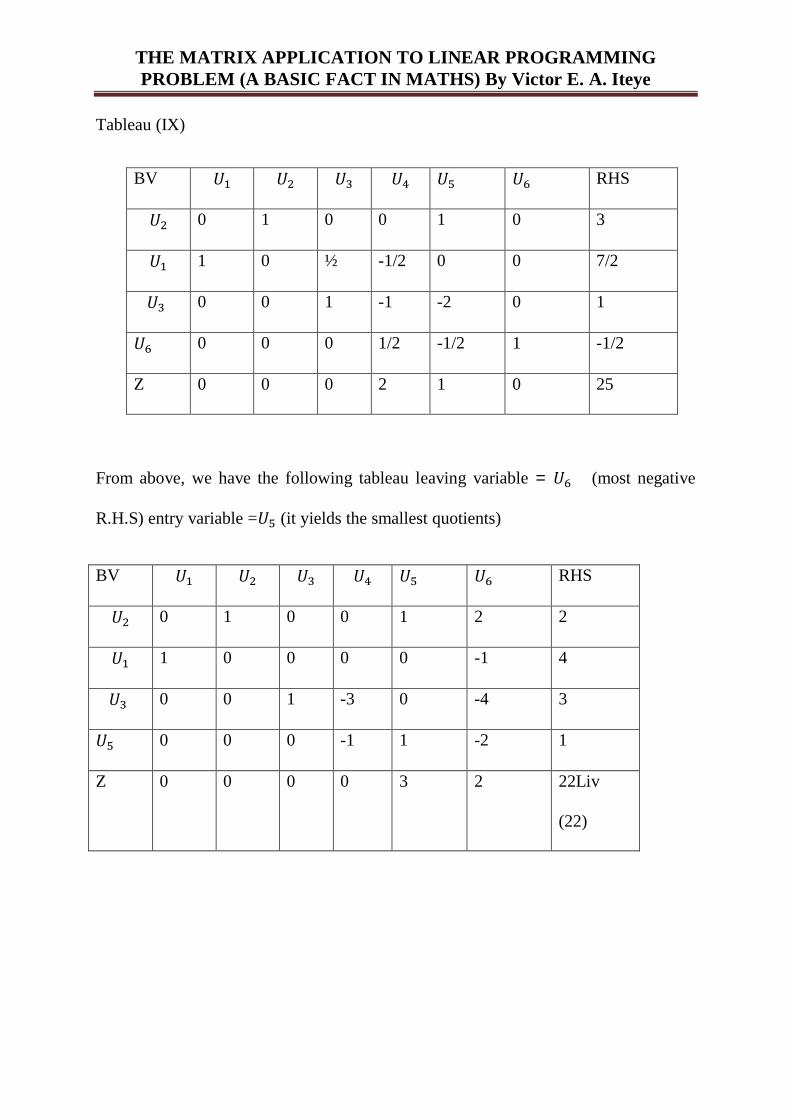
Tableau (IX)
BV 푈 푈 푈 푈 푈 푈 RHS
푈 0 1 0 0 1 0 3
푈 1 0 ½ -1/2 0 0 7/2
푈 0 0 1 -1 -2 0 1
푈 0 0 0 1/2 -1/2 1 -1/2
Z 0 0 0 2 1 0 25
From above, we have the following tableau leaving variable = 푈 (most negative
R.H.S) entry variable =푈 (it yields the smallest quotients)
BV 푈 푈 푈 푈 푈 푈 RHS
푈 0 1 0 0 1 2 2
푈 1 0 0 0 0 -1 4
푈 0 0 1 -3 0 -4 3
푈 0 0 0 -1 1 -2 1
Z 0 0 0 0 3 2 22Liv
(22)
THE MATRIX APPLICATION TO LINEAR PROGRAMMING PROBLEM (A BASIC FACT IN MATHS) By Victor E. A. Iteye
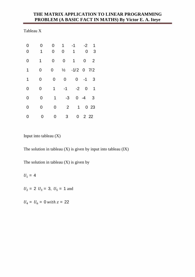
Tableau X
Input into tableau (X)
The solution in tableau (X) is given by input into tableau (IX)
The solution in tableau (X) is given by
푈 = 4
푈 = 2푈 = 3, 푈 = 1 and
푈 = 푈 = 0푤푖푡ℎ푧 = 22
0 0 0 1 -1 -2 1 0 1 0 0 1 0 3
0 1 0 0 1 0 2
1 0 0 ½ -1/2 0 7/2
1 0 0 0 0 -1 3
0 0 1 -1 -2 0 1
0 0 1 -3 0 -4 3
0 0 0 2 1 0 23
0 0 0 3 0 2 22
THE MATRIX APPLICATION TO LINEAR PROGRAMMING PROBLEM (A BASIC FACT IN MATHS) By Victor E. A. Iteye
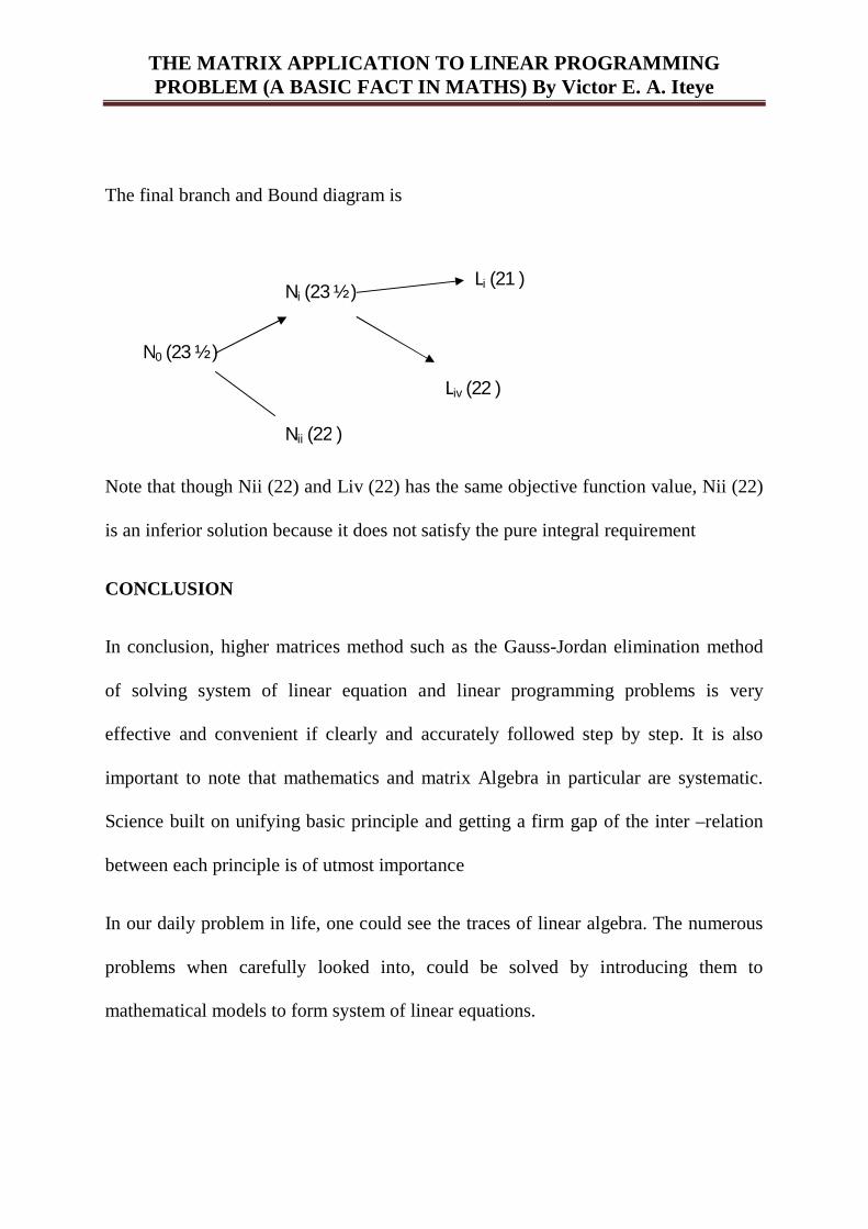
The final branch and Bound diagram is
Note that though Nii (22) and Liv (22) has the same objective function value, Nii (22)
is an inferior solution because it does not satisfy the pure integral requirement
CONCLUSION
In conclusion, higher matrices method such as the Gauss-Jordan elimination method
of solving system of linear equation and linear programming problems is very
effective and convenient if clearly and accurately followed step by step. It is also
important to note that mathematics and matrix Algebra in particular are systematic.
Science built on unifying basic principle and getting a firm gap of the inter –relation
between each principle is of utmost importance
In our daily problem in life, one could see the traces of linear algebra. The numerous
problems when carefully looked into, could be solved by introducing them to
mathematical models to form system of linear equations.
Ni (23 ½ )
N0 (23 ½ )
Nii (22 )
Li (21 )
Liv (22 )