
measurement-based characterization of large-scale
304
MEASUREMENT-BASED CHARACTERIZATION OF LARGE-SCALE NETWORKED SYSTEMS by REZA MOTAMEDI A DISSERTATION Presented to the Department of Computer and Information Science and the Graduate School of the University of Oregon in partial fulfillment of the requirements for the degree of Doctor of Philosophy December 2016
-
Upload
khangminh22 -
Category
Documents
-
view
0 -
download
0
Transcript of measurement-based characterization of large-scale

MEASUREMENT-BASED CHARACTERIZATION OF LARGE-SCALE
NETWORKED SYSTEMS
by
REZA MOTAMEDI
A DISSERTATION
Presented to the Department of Computer and Information Scienceand the Graduate School of the University of Oregon
in partial fulfillment of the requirementsfor the degree of
Doctor of Philosophy
December 2016

DISSERTATION APPROVAL PAGE
Student: Reza Motamedi
Title: Measurement-Based Characterization of Large-Scale Networked Systems
This dissertation has been accepted and approved in partial fulfillment of the requirementsfor the Doctor of Philosophy degree in the Department of Computer and InformationScience by:
Reza Rejaie ChairAllen Malony Core MemberJun Li Core MemberWalter Willinger Core MemberDavid Levin Institutional Representative
and
Scott L. Pratt Dean of the Graduate School
Original approval signatures are on file with the University of Oregon Graduate School.
Degree awarded December 2016
ii

c© 2016 Reza Motamedi
iii

DISSERTATION ABSTRACT
Reza Motamedi
Doctor of Philosophy
Department of Computer and Information Science
December 2016
Title: Measurement-Based Characterization of Large-Scale Networked Systems
As the Internet has grown to represent arguably the largest “engineered” system on
earth, network researchers have shown increasing interest in measuring this large-scale
networked system. In the process, structures such as the physical Internet or the many
different (logical) overlay networks that this physical infrastructure enables have been the
focus of numerous studies. Many of these studies have been fueled by the ease of access
to “big data”. Moreover, they benefited from advances in the study of complex networks.
However, an important missing aspect in typical applications of complex network
theory to the study of real-world distributed systems has been a general lack of attention
to domain knowledge. On the one hand, missing or superficial domain knowledge
can negatively affect the studies “input”; that is, limitations or idiosyncrasies of the
measurement methods can render the resulting graphs difficult to interpret if not
meaningless. On the other hand, lacking or insufficient domain knowledge can result in
specious “output”; that is, popular graph abstractions of real-world systems are incapable
of accounting for “details” that are important from an engineering perspective.
In this thesis, we take a closer look at measurement-based characterization of a few
real-world large-scale networked systems and focus on the role that domain knowledge
plays in gaining a thorough understanding of these systems key properties and behavior.
iv

More specifically, we use domain knowledge to (i) design context-aware measurement
strategies that capture the relevant information about the system of interest, (ii) analyze
the captured view of the networked system baring in mind the abstraction imposed by
the chosen graph representation, and (iii) scrutinize the results derived from the analysis
of the graph-based representations by investigating the root causes underlying these
findings. The main technical contribution of our work is twofolds. First, we establish
concrete connections between the amount and level of domain knowledge needed and
the quality of the measurements collected from networked systems. Second, we also
provide concrete evidence for the role that domain knowledge plays in the analysis of
views inferred from measurements collected from large-scale networked systems.
v

CURRICULUM VITAE
NAME OF AUTHOR: Reza Motamedi
GRADUATE AND UNDERGRADUATE SCHOOLS ATTENDED:University of Oregon, Eugene, ORSharif University of Technology, Tehran, IranIran University of Science & Technology, Tehran, Iran
DEGREES AWARDED:Doctor of Philosophy in Computer and Information Science,2016, University of OregonMaster of Science in Information Technology,2010, Sharif University of TechnologyBachelor of Engineering in Computer Software Engineering,2007, Iran University of Science & Technology
AREAS OF SPECIAL INTEREST:Distributed Systems, Computer Networks, Measurement, Data Science
PROFESSIONAL EXPERIENCE:
Graduate Research Fellow, Department of Computer and Information Science,University of Oregon, 2010 - present
Research Intern, Department of Computer Science, Duke University, Feb 2015 -May 2015
Network Analyst and Designer, Advanced Information & CommunicationTechnology Center, 2009
Chief Information Officer, SIEMENS SSK, 2006 - 2007
GRANTS, AWARDS AND HONORS:
Student Travel GrantCAIDA’s BGP Hackaton (San Diego) - 2016
Student Travel GrantACM Conference on Online Social Networks (San Fransisco) - 2015
vi

Julie and Rocky Dixon Graduate Innovation AwardUniversity of Oregon - 2014
Gurdeep Pall Scholarship AwardUniversity of Oregon - 2013
Clarence and Lucille Dunbar Scholarship AwardUniversity of Oregon - 2012
Student Travel GrantACM Internet Measurement Conference (Boston) - 2012
Student Travel GrantIPAM Workshop on Multi Resolution Analysis (Lake Arrowhead) - 2011
Juilf Scholarship AwardUniversity of Oregon - 2011
PUBLICATIONS:
R. Gonzalez, R. Cuevas, R. Motamedi, R. Rejaie, and A. Cuevas. Assessingthe Evolution of Google+ in its First Two Years. IEEE/ACM Transactions onNetworking (ToN), 24(3):1813–1826, 2016.
R. Motamedi, R. Rejaie, and W. Willinger. A Survey of Techniques for InternetTopology Discovery. IEEE Communications Surveys & Tutorials, 17(2):1044–1065, 2014.
R. Gonzalez, R. Cuevas, R. Motamedi, R. Rejaie, and A. Cuevas. Google+or google-?: Dissecting The Evolution of the New OSN in its First Year. InProceedings of the 22nd International Conference on World Wide Web, pages483–494. ACM, 2013.
R. Motamedi, R. Rejaie, W. Willinger, D. Lowd, and R. Gonzalez. Inferring coarseviews of connectivity in very large graphs. In Proceedings of the second ACMconference on Online social networks, COSN 2014, Dublin, Ireland, October 1-2,2014, pages 191–202. ACM, 2014.
R. Motamedi. WalkAbout – a Random Walk Based Framework to CharacterizeOSNs. In Proceedings of the Second Internet Multi-Resolution AnalysisWorkshop, Lake Arrowhead, IPAM, July 2011.
vii

M. Moshref, R. Motamedi, and H. R. Rabiee. LayeredCast – A Hybrid Peer-to-PeerLive Layered Video Streaming Protocol. In Proceedings of the fifth internationalsymposium of telecommunication, Kish, Iran, Dec, IST 2010.
viii

ACKNOWLEDGEMENTS
None of my accomplishments during the course of this eventful journey through
the years of my PhD, no matter how feeble, would have been possible without the help
and support of many. I would like to acknowledge them for their support along the way.
Above all I would like to acknowledge the tremendous sacrifices that my parents made to
ensure that I had an excellent education. Although their physical presence was lacking
from my life in the past six year, their love, devotion and support always guided me
forward. For this and much more, I am forever in their debt.
I am very grateful to my advisor Reza Rejaie who guided my research, shared his
insights and ideas, encouraged me continually and provided me with opportunities in any
possible way during the course of my time in Eugene. Working with him taught me far
more than research skills and helped me handle fasts and slows of the life of a graduate
student.
I had the privilege of having some of the most extraordinary research mentors.
I would like to thank Walter Willinger for sharing his time and invaluable experience
in research and non-research matters. His advice and recommendations were crucial
to my progress on numerous occasions. I would also like to express my gratitude to
Bruce Maggs for his mentorship and the opportunity he provided me as an intern at
Duke University. Many thanks to Ruben Cuevas for his counsel in research and genuine
friendship. I would also like to explicitly thank my committee members, Prof. Allen
Malony, Prof. Jun Li, Prof. David Levin, and Prof. Walter Willinger for taking the time
to review my dissertation and giving valuable suggestions and feedback.
Working closely with Bahador Yeganeh, Bala Chandrasekaran, and Roberto
Gonzales were some of the highlights of my life during my PhD, and the hours spent
ix

together at white boards and at lunch created friendships which I hope to keep for many
years to come. I owe special thanks to my friends and colleagues in the ONRG Lab and
other research groups at University of Oregon, including Saed Rezaei, Soheil Jamshidi,
and Pedram Rooshenas for their invaluable support and suggestions throughout my PhD
study. They were wonderful group-mates and friends and made my last few years of PhD
an enjoyable and memorable journey.
The truth is that I have had an incredible team to work with and be inspired by
throughout the course of my PhD. Each of you has contributed to my academic success
in a meaningful way, and I am sincerely grateful for your support.
x

To my dearest parents, my beloved Brandi, and all my teachers.
xi

TABLE OF CONTENTS
I. INTRODUCTION . . . . . . . . . . . . . . . . . . . . . . . . . . . . . . . . 1
1.1. Challenges and Foci in Studying Distributed Systems . . . . . . . . . 2
1.2. Over Arching Themes of the Thesis . . . . . . . . . . . . . . . . . . 3
1.3. Scope & Contributions . . . . . . . . . . . . . . . . . . . . . . . . . 4
1.4. Dissertation Outline . . . . . . . . . . . . . . . . . . . . . . . . . . 8
Part I. Online Social Networks . . . . . . . . . . . . . . . . . . . . . . . . . . . 9
II. ONLINE SOCIAL NETWORKS; BACKGROUND . . . . . . . . . . . . . . 10
2.1. Introduction . . . . . . . . . . . . . . . . . . . . . . . . . . . . . . . 10
2.2. Online Social Network as a Graph . . . . . . . . . . . . . . . . . . . 11
2.3. Comparing Online Social Networks Through Measurement . . . . . . 12
2.4. Graph Clustering & Community Detection . . . . . . . . . . . . . . 18
2.5. Identifying Key Users; Importance and Influence . . . . . . . . . . . 24
III. WALKABOUT; INFERRING COARSE VIEWS OF VERY LARGE GRAPHSUSING RANDOM WALKS . . . . . . . . . . . . . . . . . . . . . . . . . 27
3.1. Introduction . . . . . . . . . . . . . . . . . . . . . . . . . . . . . . . 28
3.2. The Behavior of Many Short RWs . . . . . . . . . . . . . . . . . . . 30
xii

Chapter Page
3.3. Detecting Regions in a Graph . . . . . . . . . . . . . . . . . . . . . 33
3.4. WalkAbout . . . . . . . . . . . . . . . . . . . . . . . . . . . . . . . 36
3.5. WalkAbout in Action . . . . . . . . . . . . . . . . . . . . . . . . . . 41
3.6. Regions vs. Communities . . . . . . . . . . . . . . . . . . . . . . . 49
3.7. A New Kind of Validation . . . . . . . . . . . . . . . . . . . . . . . 55
3.8. Summary . . . . . . . . . . . . . . . . . . . . . . . . . . . . . . . . 58
IV. CHARACTERIZING AND COMPARING GROUP-LEVEL USER BEHAVIORIN MAJOR ONLINE SOCIAL NETWORKS . . . . . . . . . . . . . . . 60
4.1. Introduction . . . . . . . . . . . . . . . . . . . . . . . . . . . . . . . 61
4.2. Methodology & Datasets . . . . . . . . . . . . . . . . . . . . . . . . 65
4.3. Crawlers . . . . . . . . . . . . . . . . . . . . . . . . . . . . . . . . 69
4.4. Connectivity & Account Age . . . . . . . . . . . . . . . . . . . . . . 72
4.5. User Activity . . . . . . . . . . . . . . . . . . . . . . . . . . . . . . 73
4.6. User Reactions . . . . . . . . . . . . . . . . . . . . . . . . . . . . . 78
4.7. Exploring Relation Among Different Group Behavior . . . . . . . . . 84
4.8. Temporal Analysis . . . . . . . . . . . . . . . . . . . . . . . . . . . 86
4.9. Summary . . . . . . . . . . . . . . . . . . . . . . . . . . . . . . . . 93
V. “WHO’S WHO” IN TWITTER . . . . . . . . . . . . . . . . . . . . . . . . . 95
5.1. Introduction . . . . . . . . . . . . . . . . . . . . . . . . . . . . . . . 96
5.2. Capturing the Elite Network . . . . . . . . . . . . . . . . . . . . . . 99
5.3. Macro-Level Structure . . . . . . . . . . . . . . . . . . . . . . . . . 105
5.4. Micro-Level Structure . . . . . . . . . . . . . . . . . . . . . . . . . 109
xiii

Chapter Page
5.5. Influence Among Elites . . . . . . . . . . . . . . . . . . . . . . . . 131
5.6. Summary . . . . . . . . . . . . . . . . . . . . . . . . . . . . . . . . 140
Part II. The Internet . . . . . . . . . . . . . . . . . . . . . . . . . . . . . . . . . 142
VI. INTERNET TOPOLOGY MAPPING; TAXONOMY & TECHNIQUES . . . 143
6.1. Introduction . . . . . . . . . . . . . . . . . . . . . . . . . . . . . . . 144
6.2. Taxonomy . . . . . . . . . . . . . . . . . . . . . . . . . . . . . . . 147
6.3. Interface-Level . . . . . . . . . . . . . . . . . . . . . . . . . . . . . 152
6.4. Router-Level . . . . . . . . . . . . . . . . . . . . . . . . . . . . . . 168
6.5. PoP Level . . . . . . . . . . . . . . . . . . . . . . . . . . . . . . . . 177
6.6. AS-Level . . . . . . . . . . . . . . . . . . . . . . . . . . . . . . . . 183
6.7. Discussion . . . . . . . . . . . . . . . . . . . . . . . . . . . . . . . 196
6.8. Summary . . . . . . . . . . . . . . . . . . . . . . . . . . . . . . . . 204
VII. POP-LEVEL TOPOLOGY OF THE INTERNET; ON THE GEOGRAPHY OFX-CONNECTS . . . . . . . . . . . . . . . . . . . . . . . . . . . . . . . 206
7.1. Introduction . . . . . . . . . . . . . . . . . . . . . . . . . . . . . . . 206
7.2. Our Approach in a Nutshell . . . . . . . . . . . . . . . . . . . . . . 208
7.3. Localized Measurements . . . . . . . . . . . . . . . . . . . . . . . . 211
7.4. Inferring AS Interconnects . . . . . . . . . . . . . . . . . . . . . . . 216
7.5. Pinning X-Connects to Facilities . . . . . . . . . . . . . . . . . . . . 229
7.6. Validation & Comparison . . . . . . . . . . . . . . . . . . . . . . . 239
7.7. Summary . . . . . . . . . . . . . . . . . . . . . . . . . . . . . . . . 244
xiv

Chapter Page
VIII.SUMMARY AND FUTURE WORK . . . . . . . . . . . . . . . . . . . . . . 247
8.1. Summary . . . . . . . . . . . . . . . . . . . . . . . . . . . . . . . . 247
8.2. Future Work . . . . . . . . . . . . . . . . . . . . . . . . . . . . . . 247
APPENDIX: ALFRED: ACQUIRING LOCATION FROM REVERSE DNS . . . . 251
A.1. ALFReD for Mining Attributes from PTR Records . . . . . . . . . . 252
A.2. ALFReD in Action . . . . . . . . . . . . . . . . . . . . . . . . . . . 257
A.3. Summary . . . . . . . . . . . . . . . . . . . . . . . . . . . . . . . . 263
REFERENCES CITED . . . . . . . . . . . . . . . . . . . . . . . . . . . . . . . . 264
xv

LIST OF FIGURES
Figure Page
2.1 The Empirical degree distribution of real OSN graphs vs. the fitted power lawdistribution. . . . . . . . . . . . . . . . . . . . . . . . . . . . . . . . . 13
2.2 Actual and randomized collaboration network of arXiv . . . . . . . . . . . 15
2.3 Actual and randomized network of a UK university faculty members . . . . 15
2.4 Visualizing two clusters of well connected nodes in a real graph . . . . . . 20
3.5 The effect of main parameters on the shape of the dvr histogram . . . . . . 30
3.6 The effect of connectivity features of a graph on the dvr histogram. . . . . . 33
3.7 Applying WalkAbout to Flickr snapshot . . . . . . . . . . . . . . . . . . . 43
3.8 Applying WalkAbout to Twitter snapshot . . . . . . . . . . . . . . . . . . 45
3.9 Applying WalkAbout to Google+ snapshot . . . . . . . . . . . . . . . . . . 47
3.10 Comparison of Louvain communities and WalkAbout regions. . . . . . . . 50
3.11 Characteristics of Louvain communities mapped to WalkAbout regions . . . 53
3.12 The comparison of the execution time for different techniques. . . . . . . . 54
3.13 Distribution of confidence in mapping groups to identified regions . . . . . 56
4.14 Basic user characteristics in different groups of each OSN. . . . . . . . . . 71
4.15 CDF of average number of daily posts per user . . . . . . . . . . . . . . . . 73
4.16 Skewness of posts/tweets contributions . . . . . . . . . . . . . . . . . . . . 73
4.17 CDF of average percentage of reshared posts per user . . . . . . . . . . . . 75
4.18 Percentage of post of each type for FB, TW and G+ . . . . . . . . . . . . . 76
4.19 CDF of average number of reactions received per user per post . . . . . . . 78
4.20 The distribution of the time between post creation & reaction across differenttarget OSNs . . . . . . . . . . . . . . . . . . . . . . . . . . . . . . . . 79
xvi

Figure Page
4.21 CDF of average number of daily reactions to posts of individual users . . . 81
4.22 The balance in the distribution of reaction across the posts . . . . . . . . . 83
4.23 Summary distribution of Likes to each type of posts for the Popular group inFB, TW and G+ . . . . . . . . . . . . . . . . . . . . . . . . . . . . . . 83
4.24 The effect 3 200 collectable tweets. . . . . . . . . . . . . . . . . . . . . . . 87
4.25 The aggregate number of posts per day . . . . . . . . . . . . . . . . . . . . 88
4.26 The aggregate number of reactions per day . . . . . . . . . . . . . . . . . . 90
5.27 The total number of nodes and edges that are reached by top-n elites. . . . . 103
5.28 PageRank of elites in 10K-ELITE grouped by their popularity rank . . . . . 104
5.29 Strongly connected components of the elite networks . . . . . . . . . . . . 107
5.30 The dynamics of LSCC as the network expands . . . . . . . . . . . . . . . 108
5.31 The number of identified resilient communities vs. number of runs . . . . . 112
5.32 Conductance vs. size of traditional and resilient communities . . . . . . . . 114
5.33 Modulairty of traditional and resilient communities . . . . . . . . . . . . . 114
5.34 The distribution of category and country in each community . . . . . . . . 116
5.35 The dynamics of communities as the elite network expands . . . . . . . . . 119
5.36 Graph structure at the community level . . . . . . . . . . . . . . . . . . . . 121
5.37 The coappearance of unstable accounts with communities . . . . . . . . . . 124
5.38 Distribution of the number of related communities for nodes in communitiesin the 10K-ELITE . . . . . . . . . . . . . . . . . . . . . . . . . . . . . 126
5.39 Using elite communities as landmarks to cluster regular users. . . . . . . . 130
5.40 Visualizing centrality captured through the social graph. . . . . . . . . . . . 133
5.41 Visualizing reaction-based influence metrics of elites. . . . . . . . . . . . . 136
5.42 Overlap among different influence measures . . . . . . . . . . . . . . . . . 138
5.43 Distribution of the popularity rank across communities . . . . . . . . . . . 139
6.44 The Internet topology at different granularities . . . . . . . . . . . . . . . . 147
xvii

Figure Page
6.45 Sample view of geo-footprint for multiple ASes . . . . . . . . . . . . . . . 152
6.46 traceroute from Host1 to Host2 and the interface-level path . . . . . . . . . 152
6.47 False links inferred by traceroute in the presence of load balancers . . . . . 155
6.48 A toy topology and corresponding subnets represented by clouds . . . . . . 166
6.49 Overlapping traceroutes with no common hops . . . . . . . . . . . . . . . 169
6.50 Graph based alias resolution . . . . . . . . . . . . . . . . . . . . . . . . . 172
6.51 False positive in graph based alias resolution due to the presence of a layer 2switch; The green interface succeeds the blue and the red interface in twotraceroute so red & blue are inferred to be aliases. . . . . . . . . . . . . 173
6.52 Analytical Alias Resolution . . . . . . . . . . . . . . . . . . . . . . . . . . 174
6.53 PoP level topology. . . . . . . . . . . . . . . . . . . . . . . . . . . . . . . 178
6.54 The PoP-level topology of Cogent . . . . . . . . . . . . . . . . . . . . . . 180
6.55 AS graph annotation with AS relations . . . . . . . . . . . . . . . . . . . . 190
7.56 An example router-level topology depicting an inter-AS x-connect. . . . . . 217
7.57 Fan-in, and Fan-out structures . . . . . . . . . . . . . . . . . . . . . . . . 218
7.58 “traceroute views” and the physical router-level topology . . . . . . . . . . 222
7.59 “traceroute views” and the physical router-level topology . . . . . . . . . . 224
7.60 The effect of c on pinning . . . . . . . . . . . . . . . . . . . . . . . . . . . 236
7.61 The effect of c on the distribution of believes for all nodes. . . . . . . . . . 237
8.62 A toy Internet topology map that encodes geographical coverage of network,the number and the location of network interconnects . . . . . . . . . . 249
A.63 Frequent domains in AS’s IP space . . . . . . . . . . . . . . . . . . . . . . 259
A.64 The distribution of the amount of information recovered by ALFReD . . . 259
A.65 Comparison MaxMind & ALFReD . . . . . . . . . . . . . . . . . . . . . . 261
A.66 ALFReD vs. its rivals . . . . . . . . . . . . . . . . . . . . . . . . . . . . . 262
A.67 ALFReD vs. its rivals . . . . . . . . . . . . . . . . . . . . . . . . . . . . . 262
xviii

Figure Page
A.68 Distribution of geo-hints not extracte by ALFReD . . . . . . . . . . . . . . 263
xix

LIST OF TABLES
Table Page
1. Characteristics of LCC snapshots of target OSNs . . . . . . . . . . . . . . 41
2. FL – Basic features of identified regions . . . . . . . . . . . . . . . . . . . 43
3. TW – Basic features of identified regions . . . . . . . . . . . . . . . . . . . 45
4. G+ – Basic features of identified regions . . . . . . . . . . . . . . . . . . . 46
5. Number of mapped communities to each region . . . . . . . . . . . . . . . 52
6. The duration of data collection for different target OSNs . . . . . . . . . . 70
7. Basic characteristics of the collected datasets for Random, Cross and Popularaccounts in all three OSNs. . . . . . . . . . . . . . . . . . . . . . . . . 71
8. Rank correlation between popularity, activity and reaction . . . . . . . . . . 84
9. Basic characteristics of the elite networks . . . . . . . . . . . . . . . . . . 106
10. General statistics of communities identified in each view. . . . . . . . . . . 113
11. The accounts that act as in/out bridges in each community. . . . . . . . . . 127
12. Top 10 most influential elites in the 10K-ELITE . . . . . . . . . . . . . . . 137
13. Different resolutions of Internet topology . . . . . . . . . . . . . . . . . . 151
14. Target CoreSite colos . . . . . . . . . . . . . . . . . . . . . . . . . . . . . 210
15. Characteristics of vantage points and destination IPs . . . . . . . . . . . . . 212
16. Details on heuristics used in each campaign . . . . . . . . . . . . . . . . . 225
17. Percentage of IPs reassigned to owner ASes of routers by different heuristicsin each campaign. . . . . . . . . . . . . . . . . . . . . . . . . . . . . . 227
18. Aggregation guidelines . . . . . . . . . . . . . . . . . . . . . . . . . . . . 228
19. The number of in- and out-anchors identified by the individual techniques foreach target colo facility . . . . . . . . . . . . . . . . . . . . . . . . . . 233
20. Sample propagation matrices for association and disassociation . . . . . . . 235
xx

Table Page
21. The number of pinned nodes of various types . . . . . . . . . . . . . . . . 240
22. The number of mapped IP-level inter-AS peerings and the aggregate numberof xconnects that they represent . . . . . . . . . . . . . . . . . . . . . . 240
23. Comparing CFS and BP . . . . . . . . . . . . . . . . . . . . . . . . . . . . 245
xxi

CHAPTER I
INTRODUCTION
In different information and technological distributed systems, there exists the
need for a monitoring and measurement of processes to analyze the health of the
platform, incorporate proper controlling mechanisms, and identify the most desired new
features of the system. In computer science research, these distributed systems cover a
wide variety of interconnected systems. Examples of such systems include but are not
limited to electric power grids, the world wide web, social networking sites, and the
Internet. The traditional approach in the research of distributed systems is to present
the relationships/interactions between the individual parts of the system as (large scale)
complex networks. The analysis, characterization, and distinction of such a complex
network in return yields insight about the distributed system that the network represents.
Recent popularity of complex networks stems from their generality and flexibility
in representing systems limited not only to man-crafted structure, but including natural
and biological systems as well. As a result, the ease of access to big data produced an
abundance of publications in this area. These studies mostly involve representing the
structure of interest as a network, followed by an analysis of the topological features of
the obtained representation performed in terms of a set of measurements. One important
missing element in the research on distributed systems casted as complex networks is the
lack of attention to domain knowledge and how the shortcomings of the measurement
approach and limitations of complex networks may affect the captured view. The extent to
which calculated measures are informative has also not been at the center of attention.
In this thesis, we take a closer look at measurement-based analysis of a few large
scale distributed systems. The emphasis on the role of domain knowledge lies at the heart
1

of this thesis. More specifically we use domain knowledge in: (i) designing a context
aware measurement strategy, (ii) analyzing the captured view of the networked system,
and (iii) investigating the root causes that lead to certain properties of the system. Our
target systems include various online social networks and the physical interconnections of
the Internet.
Challenges and Foci in Studying Distributed Systems
The Measurement and characterization of distributed systems is not without is
challenges. The most relevant challenges in this domain include:
Scale: Distributed systems are often very large. Social networks have millions of active
accounts and billions of relationships. There are approximately 40K networks in the
Internet and it is approximated that each has up to a few thousand routers. While complex
networks provide a flexible platform for the representation of these large systems,
capturing, characterizing, and analyzing these systems at scale is an open problem.
Heterogeneity: Heterogeneity of entities and subsystem proposes an additional challenge
in the study of distributed systems. For instance, in social network studies not all user
accounts are similar, as some belong to individuals and others belong to corporations.
These heterogeneities in turn effect the measurement and influence the findings.
Data: The availability and quality of data is yet another challenging aspect. Needless
to say, the study of some distributed system data is in fact considered a well-kept secret
for confidentiality and privacy reasons. While publicly available data has proven to be
a valuable source of information for researchers, more elaborate data collection tools
and techniques are often necessary to collect the most relevant information from the
system. These active data collection efforts are often limited by the API thresholds. The
2

heterogeneity of the system also imposes additional obstacles as each subsystem offers a
different API, which in turn complicates the data collection process.
Domain Knowledge: The knowledge of the context and domain governing the system
is not only necessary to the design of a proper data collection methodology, but is also
critical in characterizing and analyzing the captured view of the distributed system and
drawing informative and meaningful conclusions from the analysis. For instance, the
insight on the limitation of data collection techniques in general, the rules and attributes
of an online social network, and common practices of network operators are of great
importance in the measurement-based studies of distributed systems that we target in
this dissertation. The overall challenge is therefore the need for an extra level of “care”
to ensure the correctness of the findings inferred from the views of the distributed system
that are captured using techniques with many limitations. Indeed this level of assurance is
impossible without a sufficient amount of domain knowledge.
Over Arching Themes of the Thesis
Although we target various kinds distributed systems in our research, the design of
the measurement methodologies and analysis frameworks have many similarities.
Complex Network Analysis
Our research studies mainly fall in the category of complex network measurement
and analysis. In our analysis we often present the target system as a network (or a graph)
and aim to draw inference using this graph structure from the underlying system. We
often use graph partitioning and clustering (in Chapters III and V) to identify groups of
nodes that are tightly connected within the group and are less interconnected between
different groups. In all cases we use these groups to explain some aspect of the network
3

by analyzing the root cause for the formation of such highly knit groups. When graph
partitioning falls short, we utilize more sophisticated machine learning methods for
drawing inference over networks (in Chapter VII).
Big Data; Is More Always Better?
Another recurring theme in our research on distributed systems regards the usage of
“big data”. We argue that more data is not necessarily better and in many ways controlled
measurements can help arrive at more meaningful findings. To this end, we often take
a targeted approach to collect data from the most relevant and informative parts of any
target distributed system. Examples of such methods can be found in Chapters IV and V
where our measurement methodology allow us to find great wealth of information about a
small yet important set of users of OSNs. Similarly, in Chapter VII we demonstrate how
domain knowledge can help devise a traceroute-based campaign to uncover details of
network interconnection in a specific geographical area among a set of target networks.
Scope & Contributions
The main technical contribution of our work is the established connections between
the domain knowledge and the measurement of networked systems, and the analysis of
the views captured from complex networked systems. The following projects represent
our proposed solutions to the aforementioned problems.
Inferring Coarse Views of Connectivity in Very Large Graphs
In this research, we present a simple framework, called WalkAbout, to infer a
coarse view of connectivity in very large graphs by identifying well-connected “regions”
with different edge densities and determining the corresponding inter- and intra-region
4

connectivity. We leverage the transient behavior of many short random walks (RW)
on a large graph that is assumed to have regions of varying edge density, but whose
structure is otherwise unknown. The key idea is that as RWs approach the mixing time of
a region, the ratio of the number of visits by all RWs to the degree for nodes in that region
converges to a value proportional to the average node degree in that region. Leveraging
this indirect sign of connectivity enables our proposed framework to effectively scale with
graph size.
We demonstrate the capabilities of WalkAbout by applying it to three major OSNs
(i.e. Flickr, Twitter, and Google+) and obtaining a coarse view of their connectivity
structure. For comparison, we illustrate how the communities that are obtained by running
a popular community detection method on these OSNs stack up against the WalkAbout-
discovered regions. Finally, we examine the “meaning” of the regions obtained by
WalkAbout, and demonstrate that users in the identified regions exhibit common social
attributes.
Characterisation and Comparison of Group-level User Behavior in Major Online Social Networks
In a detailed measurement-based study to characterize and compare the behavior of
users in Facebook, Twitter, and Google+, our solution involves a “group-level” analysis.
We focus on Popular, Cross (with account in three OSNs) and Regular groups of users
in each OSN since they offer complementary views. We capture user behavior with the
following metrics: user connectivity, user activity and user reactions. Our group level
methodology enables us to capture major trends in the behavior of small but important
groups of users, and to conduct inter- and intra-OSN comparisons of user behavior.
Furthermore, we conduct temporal analysis on different aspects of user behavior for all
5

groups over a two-year period. Our analysis leads to a set of useful insights including:
(i) The more likely reaction by Facebook and Google+ users is to express their opinion
whereas Twitter users tend to relay a received post to other users and thus facilitate its
propagation. Despite the culture of reshare among Twitter users, a post by a Popular
Facebook user receives more Reshares than a post by a Popular Twitter user. (ii) Added
features in an OSN can significantly boost the rate of action and reaction among its users.
Dissecting Twitter Elite Power Network
Highest degree nodes in Online Social Networks (OSNs) such as Twitter can be
viewed as “social elites” or “connectivity hubs” as they are followed by many users and
therefore have influence over their followers. All these elites along with their pairwise
friendship relations form a structure that we refer to as “The Elite Network”. The
Elite Network serves as the backbone of the OSN structure and thus its characteristics
offer valuable insights about the core of any OSN. Despite their importance, the
characterization of elite networks has received little attention among computer scientists.
Our research presents a detailed analysis of the macro- and micro-level structure of the
Twitter elite network. Using PageRank of elites in the elite network, we show that the
Twitter elite network has an “onion-like” structure where the more popular elites are
in the center and adding less popular elites only adds to this structure’s outer layers.
Furthermore, this network is composed of a number of “communities” that exhibit strong
social cohesion. The examination of pairwise tightness between these communities
reveals the coarse structure (and level of interest) among these communities. Finally,
by exploring the aggregate influence of individual elites on other elites based on various
measures, we demonstrate that no single measure can capture all the aspects of influence.
6

Mapping X-Connects Inside a Colocation
A significant fraction of the Internet’s physical infrastructure (e.g. routers, switches,
and related equipment) is hosted at a relatively small number of physical building
complexes such as colocation facilities (or carrier hotels) and Internet eXchange Points
(IXPs). More importantly, these facilities have generally known street addresses and thus
can be accurately geo-located. Companies like Equinix, CoreSite, and Telx manage and
operate these carrier-neutral colocation facilities (also called colos) where they provide,
among other offerings, interconnection services. These facilities supply the infrastructure
(e.g. rack space, cabling, power, and physical security) necessary for network operators to
colocate their routers for easy interconnection.
This observation motivated our new methodology that is specifically designed to
map a given colo facility. This methodology relies on targeted active measurements to
identify not only all the PoPs of all the ASes present in that colo facility, but also the
corresponding inter-AS connectivity that is visible to active probing at that location. In
turn, this methodology defines a very promising, widely applicable, and highly accurate
approach for geo-locating potentially hundreds or thousands of IP addresses (i.e. all the
discovered IPs of the interfaces on the routers in the co-located PoPs) to the street address
of that facility.
This work focuses on identifying interconnections of the “x-connect” (read cross
connect) type, i.e. dedicated point-to-point private peering links (which might be used
to carry transit traffic or peer-to-peer traffic) that the network operators can buy from
the colo providers so that their networks can exchange traffic within the confines of
these facilities. In particular, our goal is to infer who is interconnecting with whom in
which colos and in which cities. Precisely locating the private peering links between
two networks is a prerequisite for studying, for example, the root causes of the peering
7

disputes between large content and eyeball providers in recent years. We illustrate the
approach with case studies of colos in Los Angles, Chicago, and Miami. These studies
demonstrate the promise as well as the challenges inherent in such a mapping effort.
Dissertation Outline
This dissertation is organized in two parts. Part I covers the material related to
the analysis of social networks and Part II focuses on discovering the topology of the
Internet. Part I is organized as follows. In Chapter II, we briefly discuss the background
and the related work on analytical measurement-based characterization of social networks
used as foundation of our own projects in Part I. Chapter III presents WalkAbout, our
proposed tool for coarsening large graphs and its application represented by three OSNs.
In Chapter IV, we present a new methodology to characterize and compare OSNs by
focusing on the behavior of diverse “groups” of users. We then show that such a group-
level cross comparison allows us to compare various aspects of the underlying OSNs
without the need for exhaustive crawls of the systems. We discuss the importance of
“Elite Power Networks” and present our methodology to effectively collect the elite
network of Twitter in Chapter V. Our detailed characterization of this network reveals
interconnection between communities of elites and allows us to identify key elite users.
Part II is composed of two chapters. Chapter VI covers a rather detailed survey
on tools and techniques for Internet topology discovery. In Chapter VII, we propose
a methodology for capturing interconnections between networks that participate in
one colocation facility to recover PoP-level maps of the topology of the Internet.
We demonstrate the applicability of our method by mapping interconnections inside
three colocation facilities. Finally, we present concluding remarks and future possible
directions for research in Chapter VIII.
8

Part I
Online Social Networks
9

CHAPTER II
ONLINE SOCIAL NETWORKS; BACKGROUND
Introduction
In the past decade, the increasing popularity of Online Social Networks (OSNs) has
led to a growing public fascination with new forms of digital connectedness. Examples
of such networks cover a variety of systems such as Email lists, discussion groups, chat
and instant messaging, audio and video conferencing, networks of financial interactions,
collaborative systems, virtual worlds and games, micro-blogging and multimedia-
blogging, and general-purpose social sharing networks. An in depth understating of an
OSN, often facilitated through complex network analysis on its social graph structure, is
essential for the evaluation of the state of the current system for social and economical
purposes. The identification of the network’s shortcomings and most critical new features
are also important. This comprehensive understanding allows researchers to synthesize
artificially crafted graphs that capture the most important features of an OSN which are
most useful for modeling purposes. For instance, the analysis on the structure of an OSN
leads to the identification of most influential and trusted users [31, 59, 43], understanding
how information diffuses over the social system [90, 154, 193, 218], designing defense
mechanisms for the system against tampering by fake users [262], or even providing
services such as web search that are not the main mission of OSNs [15, 14].
This Chapter lists the most relevant work to our studies on Online Social Networks.
After providing a brief background and context in Section 2.2, we cover a few studies
on general characterization and comparison of connectivity features, user behavior,
and temporal evolution of various OSNs in Section 2.3. In Section 2.4, we provide an
10

overview of graph clustering and community detection techniques. We then cover work
related to the identification of key users and the estimation of their influence on online
social networks in Section 2.5.
Online Social Network as a Graph
In their simplest form, online social networking sites allow (registered) users to
publish and read posts by other users. Most sites also encourage users to form friendships,
therefore allowing “friends” to automatically receive updates on the content posted
by their friends. A user can also repost others’ contents or engage in an interaction
by commenting on or replying to another user’s post. The common denominator
in the studies of OSNs is to represent the systems as graphs. These social graphs
encode relationships (e.g. friendship, repost, reply) as edges between nodes that often
represent user accounts. Depending on the OSN, social graphs can be either directed
or undirected. For instance, in Twitter many relationships are asymmetric, therefore
the graph that captures the relationship is a directed one. In order to capture a friend-
follower relationship between two users (represented by two vertex in the graph), in
which ufol follows ufri, a common encoding is to assume an edge from ufri to ufol. In this
case, messages travel along the direction of the edges on this follow graph. On the other
hand, in Facebook friendships are symmetric, therefore the social graph of Facebook can
be represented as an undirected graph. These social graphs are often referred to as the
connectivity graphs since they represent the most trivial type of relationship in the social
network.
Similar to the friendships, the interaction between users can be encoded as graphs.
As an example, in Twitter if urt retweets uorig, one can encode this relationship as a
11

directed edge from uorig to urt. Therefore, many different graph-based representations
can be derived from an OSN, each capturing one aspect of the underlying system.
Comparing Online Social Networks Through Measurement
The public popularity of OSNs spawned great interest among social and computer
scientists to monitor and characterize different aspects of these social systems [163, 254,
258, 270, 191, 190, 119]. A significant number of studies examine an OSN individually
(e.g. Twitter [163], Facebook [197], and Google+ [119]) by devising sophisticated
measurement tools for capturing (commonly referred to as crawlers) and characterizing
various aspects of the OSN. Numerous metrics have been proposed to help quantify
specific properties of these networks. Such quantitative characterization inherently
facilitates comparison between these social systems. Moreover, the growing number of
alternative social networking websites that provide similar functionalities to the most
popular OSNs motivated researchers to directly compare properties of various OSNs. The
conducted studies in this field can be broadly classified into three classes:
Social Graph & Connectivity Properties
The earliest studies on OSNs focused on characterizing their social graphs. The
commonly reported properties in all such networked systems include power law degree
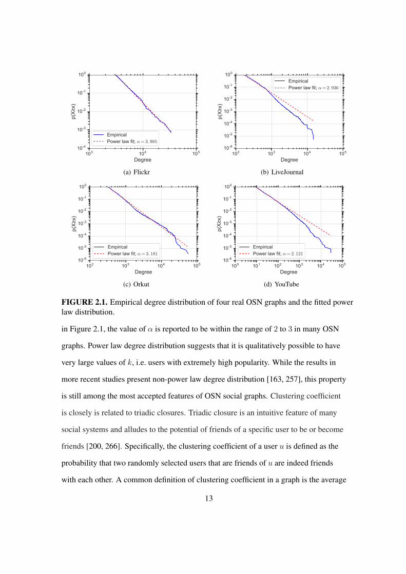
distribution1 [74], high clustering coefficient [266], and small-world properties [21].
Power law degree distribution means the fraction of nodes in the graph that have k
relationships to other nodes is proportional to k−α, in which α is the parameter of the
distribution (α > 0). Figure 2.1 demonstrates the empirical degree distribution of four
real social graphs [191] and the fitted power law distributions. As seen in the OSN graphs
1Graphs whose node degrees follows power law distribution are commonly referred to as scale-free.
12
103 104 105
Degree
10-4
10-3
10-2
10-1
100p(
Xx)
EmpiricalPower law fit; α= 3. 985
(a) Flickr
102 103 104 105
Degree
10-6
10-5
10-4
10-3
10-2
10-1
100
p(X
x)
EmpiricalPower law fit; α= 2. 936
(b) LiveJournal
102 103 104 105
Degree
10-6
10-5
10-4
10-3
10-2
10-1
100
p(X
x)
EmpiricalPower law fit; α= 3. 181
(c) Orkut
100 101 102 103 104 105
Degree
10-6
10-5
10-4
10-3
10-2
10-1
100
p(X
x)
EmpiricalPower law fit; α= 2. 121
(d) YouTube
FIGURE 2.1. Empirical degree distribution of four real OSN graphs and the fitted powerlaw distribution.
in Figure 2.1, the value of α is reported to be within the range of 2 to 3 in many OSN
graphs. Power law degree distribution suggests that it is qualitatively possible to have
very large values of k, i.e. users with extremely high popularity. While the results in
more recent studies present non-power law degree distribution [163, 257], this property
is still among the most accepted features of OSN social graphs. Clustering coefficient
is closely is related to triadic closures. Triadic closure is an intuitive feature of many
social systems and alludes to the potential of friends of a specific user to be or become
friends [200, 266]. Specifically, the clustering coefficient of a user u is defined as the
probability that two randomly selected users that are friends of u are indeed friends
with each other. A common definition of clustering coefficient in a graph is the average
13

of clustering coefficient of all users in the social graph. Alternatively, global clustering
coefficient of a graph can be defined as follows:
global clustering coefficient =3× No. of triple nodes connected by 3 edges
No. of triple nodes connected by at least 2 edges
Finally, a graph is considered small-world if its average local clustering coefficient is
higher than the randomized version of the graph, and if the graph has approximately
the same mean-shortest path length as its corresponding randomized graph (so called
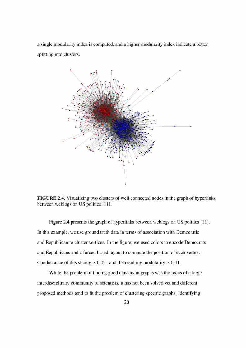
“six degrees of separation”) [266]. Figures 2.2 and 2.3 present two real sample social
graphs [198, 168] and their randomized counterparts. We applied a commonly used
rewiring technique in which each endpoint of each edge can be rewired with a constant
probability to randomize the graphs. Within the graphs, we set the rewiring probability
to 0.5. We also used forced-based layouts to visualize them [109]. We observe clear
topological structures in the form of closed triangles (three vertices that are fully
connected) and groups of well-connected vertices in the original graph. These structures
are, however, not visible in the randomized graphs. Figures also report on two metrics
in these graphs, namely clustering coefficient and average path length. We observe in
both examples that randomization clearly reduces the clustering coefficient but does not
affect the average path length. Therefore, these social graphs are examples of small-world
graphs.
The existence of these properties (or lack there of) in real social graphs has been the
focus of many studies. The connectivity properties of the social graph for Facebook [257,
29, 117], Twitter [163, 59], Google+ [178, 227, 119] and other less popular OSNs [70,
128] have been carefully analyzed recently. The results presented in these studies reveal
the social properties of the underlying system and the extent to which they resemble each
other and other social systems by comparing the quantitative metrics representing each
14
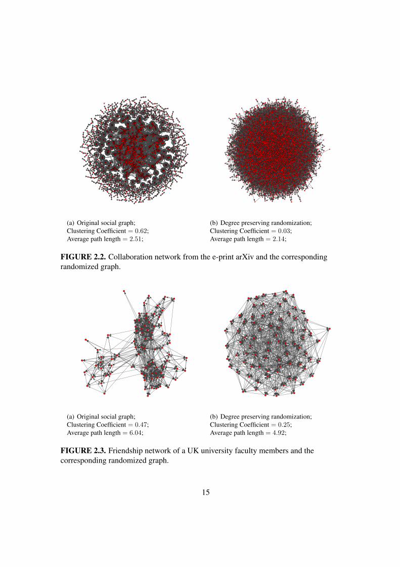
(a) Original social graph;Clustering Coefficient = 0.62;Average path length = 2.51;
(b) Degree preserving randomization;Clustering Coefficient = 0.03;Average path length = 2.14;
FIGURE 2.2. Collaboration network from the e-print arXiv and the correspondingrandomized graph.
(a) Original social graph;Clustering Coefficient = 0.47;Average path length = 6.04;
(b) Degree preserving randomization;Clustering Coefficient = 0.25;Average path length = 4.92;
FIGURE 2.3. Friendship network of a UK university faculty members and thecorresponding randomized graph.
15

social system. Some studies explicitly focus on comparing the social graphs of different
OSNs. Mislove et al. [191] analyze the graph properties for Orkut, Flickr, LiveJournal,
and YouTube. Their results confirmed the power-law and small-world properties in all
OSNs. In the same year, Ahn et al. [16] compared the topological structures of Cyworld,
MySpace, and Orkut by reporting the degree distribution, clustering property, and degree
correlation. Magno et al. [178] performed an early analysis on Google+ and identified its
main similarities and differences with other OSNs like Facebook and Twitter. Gonzalez
et al. [119] also compared the connectivity properties of the social graph of Google+,
Facebook, and Twitter. Although all the social graph of these OSNs seem to have similar
topological attributes, the small differences in them seem to render some networks more
suitable for specific purposes. For instance, it is widely accepted that Twitter is used as a
message propagation network, but Facebook is mostly used for social biding.
Users’ Behavior in Online Social Networks
Users’ behavior can also to be characterized based on real data collected from
OSNs. In particular, previous studies have used two different strategies: Passive
measurements [38, 228] and active measurements [275, 127, 119]. The former
captures traces of traffic or click streams that allow user interaction with the OSN to be
reconstructed, whereas the latter uses crawling techniques to tell “who does what” in the
system.
Gyarmati et al. [127] used active measurements to characterize user activity in the
not so popular OSNs of Bebo, MySpace, Netlog, and Tagged. They defined activity as
the time a user stays online in the system. Alternatively, a recent study by Gonzalez et al.
[120, 119] actively collected the posts contributed to Google+ by its users to characterize
the level of their interaction with the system. Another important feature of many OSNs
16

is user reaction to posts, for instance, in the form of liking or resharing a post created by
other users. In the same study, Gonzales et al. measured the amount of reaction that posts
receive. In a recent study on Pinterest, Han et al. [128] focused on the difference between
the acts of posting and reposting by considering user gender and post topics. Their results
show that in their target OSN, there is a significant variance between the frequency of
posting and reposting across topics. They also show that gender is an important factor in
the level of user engagement with the system.
These studies also commonly reported a high level of skewness withing user
activity and reaction [146]. Skewness refers to the measurement of asymmetry within a
probability distribution. Large skewness means that the mean value of the distribution
poorly captures the outliers. For instance, it has been reported that 1% of Google+
users receive more than 80% of reactions in the system [120]. Similarly, the duration
of OSN users’ online sessions exhibit high skewness and show power law distribution
characteristics. These commonly reported skewed distributions of user properties pose
additional challenges when sampling techniques are used in the characterization of social
systems.
Evolution of Online Social Networks
The evolution of OSNs has also been the focus of research in the past. The
objective of these studies is not to capture the OSN social graph as a single snapshot
at a certain point in time, but to characterize the OSN as an evolving distributed social
system, in which new user accounts are created, new friendships are formed or removed,
and content is shared through the media. The analysis of the evolution of the social graph
properties [119, 190, 16, 284, 110, 114, 217], the evolution of the interactions between
17

users [145], and the evolution of users’ availability (time spent online) over time [44] are
a few examples of such studies.
The evolution of Flickr and Yahoo! with respect to their number of users,
friendships, and the structure of their connected components was studied by Kumar et al.
[162]. Rejaie et al. [217] studied the evolution of the network size and the user activity
in MySpace and Twitter. Gonzalez et al. [119, 120] studied the growth in the number of
users and their daily activity in Google+ by capturing and monitoring the network’s main
component over the course of two years.
While studies on the evolution of OSNs primarily focus on capturing the dynamics
of the system, they also provide great insight for modeling and predicting their growth
and decline. For example, Garcia et al. [113] used snapshots of Friendster to create a
model that identifies growth patterns that result in social graph structures that are more
resilient to users’ departure.
Graph Clustering & Community Detection
One of the commonly studied aspects of graphs that represent real social systems
is detecting clusters in them or their community structure. This involves organizing
vertices in clusters (also referred to as communities, partitions, or modules) with many
edges connecting vertices of the same cluster and comparatively few edges connecting
vertices of different clusters. Finding such clusters is considered to be very important,
since each one can be considered as a fairly independent segment of a graph. In social
graphs, each community is often formed as a result of common interests of a group of
users (i.e. homophily) [186].
In the analysis of clusters in graph, one important question is how to evaluate the
“goodness” of the resulting clusters. This evaluation allows researchers to compare
18

clusters as well as the techniques that identified them. Two commonly used goodness
indexes are conductance [41] and modularity [201]. Conductance, which is a value in
[0, 1] measures how well a certain bipartition of nodes splits the graph. Therefore, for
each cut through the edges in the graph a single conductance value can be computed. For
a given cut that splits the graph into S and S, conductance (ϕ) is defined as:
ϕ(S, S) =
∑i∈S
∑j∈S ai,j
min(∑
i∈S∑
j∈V ai,j,∑
i∈S∑
j∈V ai,j)(2.1)
in which aij = 1 if an edge exists between vertex i and j. A small conductance index
means few edges are cut in order to split the graph into two halves (i.e. the community
and the rest of the graph).
On the other hand, modularity measures how well a graph divides into clusters.
In other words, a graph with high modularity computed for a certain grouping of nodes
into clusters have dense connections between the nodes within modules, but sparse
connections between nodes in different modules. Modularity (Q) of the graph G over
grouping C is defined as follows:
Q(G, C) =k∑i=1
(eii − a2i ) (2.2)
in which k is the number of communities in C, eii is fraction of edges in community i,
and ai is the fraction of edges with at least one side in community i. Using the above
definition, modularity essentially measures the fraction of the edges in the network that
connect vertices in the same cluster minus the expected value of the same quantity in the
randomized version of the graph. Therefore, for each graph partitioning into communities
19
a single modularity index is computed, and a higher modularity index indicate a better
splitting into clusters.
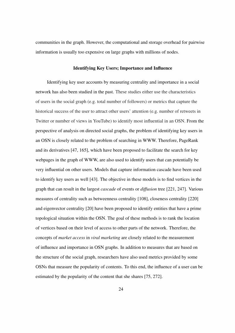
FIGURE 2.4. Visualizing two clusters of well connected nodes in the graph of hyperlinksbetween weblogs on US politics [11].
Figure 2.4 presents the graph of hyperlinks between weblogs on US politics [11].
In this example, we use ground truth data in terms of association with Democratic
and Republican to cluster vertices. In the figure, we used colors to encode Democrats
and Republicans and a forced based layout to compute the position of each vertex.
Conductance of this slicing is 0.091 and the resulting modularity is 0.41.
While the problem of finding good clusters in graphs was the focus of a large
interdisciplinary community of scientists, it has not been solved yet and different
proposed methods tend to fit the problem of clustering specific graphs. Identifying
20

clusters in graphs can be broadly categorized into two categories. In a global clustering,
each vertex of the input graph is assigned a cluster in the output, whereas in a local
clustering, the cluster assignments are performed with respect to a certain subset of
vertices in the graph to create a bi-partitioning of the input graph.
Local Graph Clustering: Local clustering methods aim to detect a tightly interconnected
partition around a given seed vertex. The time complexity of most algorithms that fill
in this category are proportional to the size of the local cluster and not the entire graph.
Local graph partitioning using PageRank [22] is one of the most popular approaches in
this domain. In this method, first a localized PageRank vector is used to rank vertices
based on their distance (similarity) to the seed vertex. Then a sweep over this ordering
is used to find a set of vertices that minimizes the normalized cut (conductance) and
therefore results in a good bi-partitioning.
A few prior studies have used RWs to distinguish local clusters. For instance, to
distinguish sybil from trusted accounts in an OSN, random walks are used to measure
accounts’ relative connectivity from trusted vertices [58, 263]. Therefore the algorithm
divides users into two groups; a group that falls within the local cluster and the rest of
vertices that do not.
Global Graph Clustering: The general goal underlying global clustering methods is
to produce a grouping of nodes into modules (also referred to as clusters, communities,
partitions) that is optimal (or close to optimal) with respect to a given cluster quality
measure [107, 164, 129]. Uncovering the community structure exhibited by networks is a
crucial step in understanding the complex systems. Many algorithms have been proposed
that show great potential in detecting communities within small to mid-size networks that
are sometimes artificially generated and therefore have known community structures.
The two main classes of approaches in this field are community detection and graph
21

partitioning. While community detection methods perform bottom-up clustering, graph
partitioning methods typically perform in a top-down fashion by splitting the graph into
sets of nodes with low interconnections [149, 41].
Most methods work by optimizing an objective function. Since this is typically
NP-hard, greedy or heuristic methods are usually necessary. One of the most popular
metrics for community detection is modularity, which relates the number of edges
within clusters to the expected number for a random graph. Louvain method [40] is
one of the most scalable and effective algorithms that aims at optimizing modularity. It
greedily assigns nodes to communities based on their local connectivity, then coarsens
the graph by replacing each community with a single node. This procedure repeats until it
reaches a local optimum of modularity. However, in most real-world graphs, modularity
tends to favor smaller communities of around 100 nodes [169]. Other measures such
as conductance also tend to favor small clusters in real-world graphs, limiting their
effectiveness at describing high-level structure.
Graph partitioning techniques [150, 151] adopt a top-down approach. These
techniques divide the vertices in groups of predefined size, such that the number of
edges lying between the groups is minimal. These methods optionally recurse within
each partition to obtain the desired granularity [88, 150, 151]. While this does discover
larger regions than the bottom-up approaches, these regions may or may not faithfully
represent the overall graph structure. For example, methods that optimize the popular
normalized cut criterion tend to produce regions of approximately equal size, even when
this leads to poorly separated regions. Furthermore, some approaches require specifying
seed instances for each partition [22] or the total number of partitions, both of which can
be difficult to determine a priori. Finally, many of these techniques, including spectral
22

clustering [149], do not scale with graph size and often require a complete snapshot of the
target graph or its adjacency matrix.
Spectral clustering techniques attempt to partition a graph into dense groups
of nodes, for instance by minimizing the normalized cut. These techniques typically
involve finding eigenvectors of the adjacency matrix of a graph or one of its derivatives.
This transforms the initial set of vertices into points in the space whose coordinates
are elements are eigenvectors. Classical clustering techniques such as K-means [170]
can then be used to cluster vertices. The main complexity of these techniques lies in
the calculation of eigenvectors which is computationally expensive (O(n3)). There are
more scalable alternatives which do not use eigenvectors (Graclus [84]) or approximate
them instead by using techniques such as power method. However, methods based on
the normalized cut tend to create clusters whose sizes are known a priori (often time
balanced), which may lead to clusters that are not well-separated since the provided sizes
are not correct.
The Markov clustering algorithm (MCL) [260] has proven particularly effective for
finding structure in biological networks. It works by defining and iteratively refining a
stochastic flow until each node has a non-zero flow to just one other node. Nodes with the
same target are grouped into the same community. The main limitation of MCL is its poor
scalability with the graph size. MLR-MCL [225] is a multi-level, regularized variant of
MCL that improves the scalability and quality of MCL.
Some proposed algorithms use random walks and “flows” [259, 213, 225, 130]
for community detection. The random walk or the associated transition matrix are used
to compute a measure of distance between all pairs of nodes. This distance measure
is in turn used to cluster groups of nodes that are closer to each other, and hence find
23
communities in the graph. However, the computational and storage overhead for pairwise
information is usually too expensive on large graphs with millions of nodes.
Identifying Key Users; Importance and Influence
Identifying key user accounts by measuring centrality and importance in a social
network has also been studied in the past. These studies either use the characteristics
of users in the social graph (e.g. total number of followers) or metrics that capture the
historical success of the user to attract other users’ attention (e.g. number of retweets in
Twitter or number of views in YouTube) to identify most influential in an OSN. From the
perspective of analysis on directed social graphs, the problem of identifying key users in
an OSN is closely related to the problem of searching in WWW. Therefore, PageRank
and its derivatives [47, 165], which have been proposed to facilitate the search for key
webpages in the graph of WWW, are also used to identify users that can potentially be
very influential on other users. Models that capture information cascade have been used
to identify key users as well [43]. The objective in these models is to find vertices in the
graph that can result in the largest cascade of events or diffusion tree [221, 247]. Various
measures of centrality such as betweenness centrality [108], closeness centrality [220]
and eigenvector centrality [20] have been proposed to identify entities that have a prime
topological situation within the OSN. The goal of these methods is to rank the location
of vertices based on their level of access to other parts of the network. Therefore, the
concepts of market access in viral marketing are closely related to the measurement
of influence and importance in OSN graphs. In addition to measures that are based on
the structure of the social graph, researchers have also used metrics provided by some
OSNs that measure the popularity of contents. To this end, the influence of a user can be
estimated by the popularity of the content that she shares [75, 272].
24

Since influence and importance have many aspects, many studies used multiple
metrics to capture them. Kwak et al. [163] ranked Twitter users by (i) their number
of followers, (ii) PageRank computed over the social graph and, (iii) their number of
retweets to identify the most influential users. They reported a higher correlation between
the number of followers and PageRank metrics compared to the correlations among other
pairs of metrics2. Welch et al. [267] computed PageRank over both graph and social
graphs, and then compared the resulting rankings. They concluded that PageRank over
the social graph reveals the popularity of a user and PageRank over the retweet graph
demonstrates user influence. However, since their retweet graph has a direct edge from
the original sender to each retweeting user (essentially a collection of a number of star-
graphs), it does not capture the diffusion of the tweet and thus the resulting PageRank
on the retweet graph does not reveal a correct measure of influence. To overcome this
issue, some studies tried to heuristically reconstruct the diffusion tree using the timing of
the reposts and the friendships among users that are invalided in the diffusion [30, 60].
Backshy et al. [30] tried to predict individual influence by predicting how an individual
can start a cascade event of a certain size and depth. To do so, they first proposed a
technique to reconstruct the retweet diffusion tree using the entire social graph. However,
due to the limited data collection capacity, they used an old snapshot of the social graph
that was captured approximately 10 months prior to the retweet events. This timing gap
potentially leads to error in retweet tree reconstruction. Cogan et al. [75] studied user
interactions on Twitter. They designed an algorithm to reconstruct the conversational
graphs (mentions, retweets, replies). Their goal was to reconstruct cascade trees that
capture interactions between individual users, and measure the influence of a user based
on the cascades that started from each user. Deng et al. [81] argued that past history is
2This higher level of correlation seems inherent since PageRank centrality and degree centrality aregreatly correlated.
25

not sufficient when measuring influence. Instead, they assume that users are primarily
influenced by their friends. Using the social graph of Weibo (Chinese Twitter) and retweet
information, they used a Baysian method to estimate the pairwise influence of users
(influence over each edge) and therefore predict the properties of new diffusion trees.
Wu et al. [272] also studied the influence on Twitter. However, their main focus is to
capture “who listens to whom on Twitter” and report that conventional media sources
with large number of followers play a different role in message propagation to regular
users compared to other online celebrities.
26

CHAPTER III
WALKABOUT; INFERRING COARSE VIEWS OF VERY LARGE GRAPHS USING
RANDOM WALKS
This chapter presents a simple framework, called WalkAbout, to infer a coarse
view of connectivity in very large graphs; that is, identify well-connected “regions”
with different edge densities and determine the corresponding inter- and intra-region
connectivity. We leverage the transient behavior of many short random walks (RW)
on a large graph that is assumed to have regions of varying edge density but whose
structure is otherwise unknown. The key idea is that as RWs approach the mixing time of
a region, the ratio of the number of visits by all RWs to the degree for nodes in that region
converges to a value proportional to the average node degree in that region. Utilizing this
indirect sign of regional connectivity enables our proposed framework to effectively scale
with graph size.
After describing the design of WalkAbout, we demonstrate the capabilities of
WalkAbout by applying it to three major OSNs (i.e. Flickr, Twitter, and Google+) and
obtaining a coarse view of their connectivity structure. In addition, we illustrate how the
communities that are obtained by running a popular community detection method on
these OSNs stack up against the WalkAbout-discovered regions. Finally, we examine
the “meaning” of the regions obtained by WalkAbout, and demonstrate that users in the
identified regions exhibit common social attributes.
WalkAbout is different from the prior approaches in graph clustering as it is not
optimizing a single metric or objective function. Rather, it is a heuristic approach that
relies on an interesting transient phenomenon to explore the coarse view of structure in
very large graphs. More specifically, WalkAbout does not only produce a single coarse
27

view of connectivity, but also its parameters allow a user to explore the connectivity
structure to identify proper view at the desired resolution.
Introduction
Large-scale, networked systems such as the World Wide Web or Online Social
Networks (OSNs) can be represented as graphs where nodes represent individual entities,
such as web pages or user accounts, and directed or undirected edges represent relations
between these entities, such as interaction or friendship between users [159, 191, 249].
Characterizing the connectivity structure of such a graph, in particular at scale, often
provides deeper insight into the corresponding networked system and has motivated many
researchers to analyze graph representations of large networked systems (e.g. [16]).
It is often very useful to obtain a coarse view of the connectivity structure of a
huge graph that shows a few major tightly connected components or regions of the graph
along with the inter- and intra-region connectivity. Such a regional view also enables
a natural top-down approach to the analysis of large graphs, where one first examines
the regional connectivity of a huge graph and then zooms in to individual regions to
explore their structure in further detail. However, capturing a regional view of a huge
graph is a non-trivial task that existing tools and techniques are not able to achieve.
While many techniques exist for graph clustering [268, 83], graph partitioning [150], and
community detection [40, 213, 107], these approaches do not work well for discovering
coarse regional views in very large graphs. These methods usually scale poorly, force
regions to have similar size, or find communities that are too small. For example, existing
techniques (e.g. Louvain [40]) are likely to identify tens of thousands of communities in
the structure of a large OSN that is still too complex for high-level analysis to determine
the full picture of inter-community connectivity.
28

This chapter presents a simple top-down framework, called WalkAbout, to identify
tightly connected regions in a large unknown graph and subsequently characterize the
regional view of its connectivity structure. The main idea is to leverage the behavior of
an army of short random walks (RW) on a graph to identify nodes that are located in the
same region. When the random walks are longer than the mixing time of an individual
region and shorter than the mixing time of the overall graph, the ratio of node degree to
expected number of visits is proportional to the edge density of that region. We refer to
this quantity as the degree/visit ratio (dvr). If individual regions in a graph have different
edge densities and shorter mixing times than the entire graph, we can leverage the dvr
“signal” to identify the regions, their corresponding nodes and their intra- and inter-
region connectivity. The main novelty of WalkAbout is to leverage this indirect sign
of connectivity to identify tightly connected nodes in a region. This leads to a very
scalable method: in a graph with |V | nodes, |E| edges, and a regional mixing time of
wl, WalkAbout requires only O(wl × |E|) time and O(|V |) space. A few parameters in
WalkAbout enable one to explore different aspects of the regional connectivity in order to
produce the outcome with the desired resolution.
In our empirical evaluation, we apply WalkAbout to three major OSNs: Flickr,
Twitter and Google+. Compared to Louvain [40], the gold standard for scalable
community detection, WalkAbout runs faster and finds larger, coarser regions. Most
communities discovered by Louvain can be mapped to a single one of WalkAbout’s
regions, suggesting that WalkAbout is providing a higher-level view of the network
than Louvain. Finally, we analyze the regions in Flickr and show that different regions
discovered by WalkAbout correspond to different interest groups, providing a meaningful
coarse view of this OSN.
29

40 45 50 55 600
0.05
0.1
0.15
0.2P
DF
dvr
wl=10
wl=20
wl=50
wl=100
(a) Walk length
44 46 48 50 52 54 560
0.05
0.1
0.15
0.2
PD
F
dvr
smw prob=0.01
smw prob=0.02
smw prob=0.04
smw prob=0.08
(b) Graph mixing time
10 20 30 40 50 600
0.05
0.1
0.15
0.2
PD
F
dvr
Avg. degree=24.74
Avg. degree=33.94
Avg. degree=44.30
Avg. degree=53.29
(c) Average node degree
40 45 50 55 600
0.05
0.1
0.15
0.2
PD
F
dvr
MinDeg=0
MinDeg=25
MinDeg=50
MinDeg=75
(d) Minimum degree
10 30 50 7040
45
50
55
60
wl
dvr
deg<50
deg>100
(e) Effect of node degree
FIGURE 3.5. The effect of main parameters on the shape of the dvr histogram
The remainder of this chapter is organized as follows. Section 3.2 explores the
behavior of short random walks and dvr on graphs with a single region. Section 3.3
extends this analysis to multiple region graphs and motivates using dvr for region
identification. In Section 3.4, we present the full details of WalkAbout, our step-by-
step framework for identifying regions in large graphs. To demonstrate and evaluate
WalkAbout, we apply it to three major OSNs in Section 3.5. In Section 3.6, we compare
the characteristics of Louvain communities with WalkAbout regions. We show that the
regions discovered by WalkAbout are indeed meaningful in Section 3.7. We conclude the
chapter in Section 3.8 and summarize our future plans.
The Behavior of Many Short RWs
Random Walks (RW) are a well-known technique for sampling graphs. A RW
on a graph starts from an arbitrary node and at each step moves to a randomly chosen
30

neighbor of the current node. Consider a graph G = [V,E] where V and E denote
the set of graph vertices and edges, respectively. In an undirected, connected, and non-
bipartite graph, the probability that a sufficiently long RW would be at a particular node
x converges to deg(x)2×|E| [173]. The mixing time TG(ε) of a graph G is the walk length at
which the probability of being at each node is within ε of the stationary distribution. In
this chapter, we will use this term somewhat informally, without specifying a particular
value of ε.
Suppose we run |V | RWs in parallel, one starting at each node. Let V (x,wl) denote
the expected number of RWs that are at a particular node x after wl number of steps (e.g.,
walk length of wl). Since one RW is started at each node, V (x, 0) = 1. For other values
of wl, we can define V (x, k) inductively:
V (x, 0) = 1
V (x,wl) =∑
n∈Neighbors(x)
V (n,wl − 1)
deg(n)for wl > 0 (3.1)
This function can be computed iteratively with complexity O(|E|wl). As wl
reaches the mixing time, V (x,wl) converges to |V |deg(x)2×|E| . Hence, when wl is sufficiently
long, the following holds for all nodes:
deg(x)
V (x,wl)≈ 2× |E|
|V |(3.2)
We refer to the fraction deg(x)V (x,wl)
as the degree/visit ratio or dvr. Equation (2)
indicates that the dvr converges to the average degree of the graph.
In practice, estimating the mixing time for an arbitrary graph is a known
hard problem. In this section, we will explore the dependency of dvr on wl through
31

simulations on different synthetically-generated graphs. The graphs are generated by
selecting the range of node degrees, the distribution of node degrees across this range,
and then randomly connecting the nodes until all half-edges are connected. For each
simulation, we show a normalized histogram of dvr values across all nodes, which
represents the empirical distribution of dvr values for that simulation.
Effect of Walk Length: Figure 3.5(a) shows the evolution of the dvr histogram as we
increase walk length over a generic random graph. As the walk length increases, the
variation in dvr across different nodes decreases, leading to the formation of a narrower
peak in the histogram. As wl reaches the mixing time, the probability of visiting each
node becomes approximately proportional to its degree.
Effect of Mixing Time: To explore the effect of mixing time on the dvr histogram, we
show in Figure 3.5(b) the evolution of the dvr histogram for a small-world graph as we
increase the level of clustering (and thus the mixing time) for a particular walk length
(wl = 20). As the mixing time becomes longer, the variation in dvr values increases
because the RWs are farther from convergence.
Effect of Average Node Degree (E): Figure 3.5(c) presents the effect of average node
degree (i.e. changing |E| when |V | is fixed) on the shape of the dvr histogram at a given
walk length (wl = 20). Increasing the average node degree shifts the corresponding
peak to higher dvr values. It is worth noting that the placement of each peak is in perfect
agreement with the average degree of each graph.
Effect of Minimum Node Degree: Figure 3.5(d) shows the contribution of low degree
nodes to the shape of the dvr histogram by plotting the histogram only for nodes whose
degree is larger than a threshold Dmin. We find that higher degree nodes show less
variation in dvr than low degree nodes, i.e. filtering low degree nodes leads to a sharper
peak in the histogram. Figure 3.5(e) depicts the evolution of summary distribution of dvr
32

20
40
60
80
50
55
60
650
0.01
0.02
0.03
dvrAvg. Degree
PD
F
(a) Changing edge density of oneregion
20
40
60
80
2000
4000
6000
80000
0.01
0.02
0.03
Region Size
PD
F
(b) Changing the size of oneregion
20
40
60
80
12
34
5
x 104
0
0.01
0.02
0.03
dvrBridge Size
PD
F
(c) Changing the num. of bridgeconnections
FIGURE 3.6. The effect of connectivity features of a two-region graph on the dvrhistogram (wl = 20)
across two groups of nodes with different degrees which shows that the range of dvr is
inversely proportional with node degree and rapidly decreases with the walk length. This
property is due to the fact that higher degree nodes are averaging over more neighbors in
each update of V (x,wl), thus reducing the variation.
Detecting Regions in a Graph
To infer a coarse view of graph connectivity, we assume that each graph consists
of a number of weakly inter-connected regions, where individual regions have varying
edge density. We use the term “region” instead of “community” to emphasize the fact that
regions are often much larger in size than typical communities, and are identified based
on a heuristic rather than optimizing an objective function or a metric.
We have no a priori knowledge of either the number of regions or their relative
size and make no assumptions about the precise nature of the inter-region connectivity or
intra-region connections.
33

The Key Idea
Our approach is to leverage the behavior of RWs that are shorter than the mixing
time of the graph to identify nodes in each region of the graph. To this end, consider RWs
that start from randomly selected nodes of a graph G = [V,E] that has multiple regions.
Based on our discussion in Section 3.2, the fraction of RWs that start in region i (Gi =
[Vi, Ei]) of the graph is equal to the fraction of nodes in that region (i.e. |Vi||V | ). If the length
of those RWs is approximately equal to the mixing time of regions Gi, a majority of RWs
will remain within that starting region, and for all practical purposes, we can view the
different regions of the graph as disconnected partitions. Thus, we can use Equation (3.2)
to determine the value of the dvr ratio to which node x in region i converges to as follows:
dvri(x) =deg(x)
E[V (x,wl)]=
(2× |Ei|)|Vi|
, (3.3)
Equation 3.3 shows that the degree-to-visit ratio for nodes x in region i equals
2×|Ei||Vi| which is the average node degree for region i. Therefore, if regions of the graph
have different average node degrees, the dvri(x) values for nodes in each region converge
to a different dvr value, i.e. form a peak at a different location in the dvr histogram across
all nodes. We can represent each region with its associated non-overlapping range of dvr
values and then map visited nodes to a region based on their dvr values. Furthermore, as
discussed earlier, other key connectivity features of a region i (e.g. mixing time and size)
affect the shape of the corresponding peak.
As the length of the RWs increases beyond the mixing time of individual regions,
the RWs are likely to leave their starting regions and contribute to the number of
visits for nodes in other regions of the graph. This in turn decreases the gap in the
34

dvri(x) values for different regions and the dvr values for all nodes converge to a single
value (determined by Equation (3.2)) as soon as the walk length of the RWs agrees
approximately with the mixing time of the entire graph. Therefore, the separation
between peaks in the dvr histogram that are associated with different regions of a graph
is a transient phenomenon that occurs for RWs whose walk lengths are between region-
specific mixing times and the mixing time for the entire graph. The more pronounced the
regions, the larger the gaps between the mixing times of individual regions and the entire
graph, which in turn translates to a longer transient phase and simplifies the detection of
different regions. In a nutshell, the similarity in dvr value serves as a promising indirect
signal that reveals a tight connectivity among a group of nodes in a graph. The indirect
nature of the dvr signal coupled with the ability to efficiently obtain dvr values using short
random walks enables our approach to scale with graph size.
Validation with Synthetic Graphs
Next we use synthetic graphs to demonstrate how our basic idea can reveal (or
decode) the regional connectivity features within a graph. To this end, we consider a
graph G with two regions, R0 and R1, both with 4K nodes and random connectivity
and an average degree of 70 and 60, respectively. We connect these two regions with b
bridge connections, where each bridge connection is between a pair of random nodes
from these regions, and its default value is b=10k. In essence, the value of b controls the
inter-region connectivity and thus the mixing time of the entire graph. To illustrate the
effect of regional connectivity features on the shape of the dvr histogram, we keep region
R0 fixed and systematically change features of R1 and the value of b.
Figure 3.6(a) shows the evolution of the dvr histogram as we vary the average node
degree in R1 between 50 and 66. We observe that as the average degree of R1 increases,
35

the corresponding peak gradually moves to higher dvr values and blends into the peak for
R0 until individual peaks are no longer distinguishable. Figure 3.6(b) shows how varying
the size of R1 from 1K to 8K nodes affects the shape of the dvr histogram when all other
parameters remain constant. Increasing the size of a region proportionally increases
the number of RWs that start from that region which in turn leads to a proportionally
larger peak. Since we normalize dvr and plot the PDF, the peak corresponding to R0
decreases in size. Finally, Figure 3.6(c) illustrates the effect of increasing the number
of bridge edges (or bridge width) between the two regions from 5K to 50k. We note that
as the bridge width increases, the two peaks gradually merge and become less and less
distinguishable. This is due to the fact that increasing bridge width decreases the mixing
time of the entire graph and thus shrinks the transition phase where the peaks for two
regions can be clearly identified.
In summary, these examples illustrate that the behavior of many short RWs on a
single graph can be extended to multi-region graphs as long as the mixing time of the
entire graph is sufficiently larger than the the mixing time of individual regions.
WalkAbout
In this section, we present WalkAbout, our proposed method for inferring and
exploring a regional (i.e. coarse) view of connectivity for large graphs. We first discuss
some of the basic challenges in designing such a methodology and then describe our
approach and how it addresses these challenges.
Basic Challenges
The behavior of many short RWs on a large graph motivates the idea of using
the similarity of dvr values to identify individual regions of a graph where regions
36

are represented as a collection of nodes with non-overlapping ranges of dvr values.
To implement this idea in practice, a number of challenges arise. First, we recall that
the variation of dvr values across nodes with degree d in a given region decreases
monotonically while the median value converges towards the average node degree of the
region. More importantly, the degree of variation and its rate of convergence is inversely
proportional to the node degree d, i.e. dvr values of higher degree nodes exhibit smaller
variations and convergence faster than lower degree nodes. The typically large fraction of
low degree nodes in big graphs coupled with the wider variation and slower convergence
rate of their dvr values make it difficult to accurately associate a set of nodes with their
corresponding region. This problem is further exacerbated by the fact that different
regions may have a different mixing time and overlapping ra nges of dvr values.
Main Steps of WalkAbout
Given a large graph G[V,E], the goal of WalkAbout is to identify the number
of regions, map all nodes to their corresponding region, and determine the inter- and
intra-region connectivity (i.e. fraction of edges that are connecting nodes in different
regions or the same region). We call such a representation of a large graph a regional (or
coarse) view of the graph. To overcome the above-mentioned challenges, WalkAbout
identifies individual regions in two steps. First, it identifies a “core” component for
each region. Such a component consists of a collection of high degree nodes in that
region based on the similarity of their dvr values. Second, it considers each of these
core components, views their elements as “anchors” and maps the remaining low degree
nodes to the various regions based on the nodes’ relative reachability to each core. This
approach can effectively cope with the variations of the dvr values for low degree nodes
and is less sensitive to the walk length. The WalkAbout technique comes with a set of
37

parameters/options that enable the exploration of the regional connectivity of a graph
and support experimentation with different coarse views of a graph. In the following, we
describe the five main steps of the WalkAbout technique.
1) Determining dvr Values for Individual Nodes: We emulate the behavior of |V | short
RWs starting from individual nodes in the graph and derive the probability of visits and
use that probability to determine the degree-to-visit ratio for individual nodes at walk
length wl, similar to Equation (1).
2) Creating the dvr Histogram: Given the dvr values of different nodes , our goal
is to group nodes with similar dvr values and use them as the core elements for the
corresponding region. To this end, we bin the nodes based on their dvr values and
generate a histogram to identify the most common values (i.e. “peaks”) which in turn
suggest the existence of different regions. To reduce the noise that the wide variation of
dvr values for low degree nodes introduces, we first filter out all nodes whose degree is
smaller than a threshold Dmin. In fact Dmin is a parameter that can be used to control
the visibility of nodes that are under possible consideration for being selected as core
elements. It provides a knob for examining the trade-offs that result from increasing the
level of noise caused by a larger number of low degree nodes (i.e. small Dmin values) –
allowing for more noise typically results in the identification of a larger number of less
reliable core elements and hence regions. Next, while the dvr values for higher degree
nodes are significantly more reliable, these nodes may not have a profound impact on
the shape of the histogram due to the often small fraction of high degree nodes. We
deal with this issue by introducing a bias towards the dvr v alues of high degree nodes.
In particular, for each high degree node, we multiply its dvr value by its node degree.
In effect, we simply increase the frequency of the dvr values of the high degree nodes
proportional to their node degree. The resulting conditioned histogram is in general more
38

amenable to reveal the presence of reliable regions since it has more pronounced peaks
that are less sensitive to the value of Dmin parameter.
3) Identifying Core of a Region From the Histogram: Identifying regions from a
dvr histogram requires (i) determining a proper walk length that generates the best
histogram, and (ii) detecting the regions from the resulting histogram. To deal with item
(i), we progressively increase the walk length and repeat steps (1) and (2) to generate the
resulting histogram. We carefully examine the evolution of the histogram as a function
of walk length and select the histogram where the peaks are most pronounced and most
separated. By definition, such a histogram should be formed when the walk length is
close to the mixing time of individual regions. In such a histogram, each peak (i.e. a
local maximum that is surrounded by two local minimum values) represents a region’s
core whose range of dvr values is specified by the dvr values corresponding to the two
minimum values. This heuristic can be viewed as a naive one-dimensional clustering
technique. We examine the connectivity among nodes that are part of each core to ensure
that they form a connected component1. This check also reveals whether the cores of
two separate regions with overlapping dvr ranges appear as a single peak which makes it
difficult to distinguish them from the histogram in the first place. At the end of this step,
we have the number of regions and the list of high degree nodes that form the core of each
region.
4) Mapping Low-Degree Nodes to Cores: We use the relative reachability of low degree
nodes to identified cores in order to map them. To this end, we start N RWs from each
node where each RW walk continues until it hits a node in one of the cores. Each walk
provides a sample of reachability for this node. The node is mapped to the core with the
1It is not a required condition that core nodes form a connected component. However, forming aconnected component does indicate that the core is coherent.
39

highest reachability. The fraction of RWs that hit the most reachable core indicates our
confidence in mapping a node to that region.
5) Producing the Regional View: Once nodes in each region of the graph are identified,
we determine the edges that are within each region or connecting two different
regions. Then we produce a diagram that incorporates all the information about
regional connectivity of a graph including (i) a circle represents a region with the area
logarithmically proportional to the size of the region, (ii) arrows between two regions
indicate the inter-region connectivity and their width as well as color is proportional with
the relative fraction of directed half-edges between two regions. Intra region half-edges
are represented with the modularity of a region and thus are not shown in the regional
view to keep this less crowded.
Inferring vs. Exploring Regions
The design of WalkAbout provides several parameters or knobs that can be tuned
to explore different coarse views of a given graph. These parameters include the walk
length, the Dmin threshold, and the precise nature of determining how low degree
nodes get mapped to regions (core anchors). In essence, examining the effect of these
parameters on the resulting regional views facilitates studying the quality of a given
regional view in terms of its robustness to the choices WalkAbout offers to its users. In
this sense, WalkAbout can be viewed as a framework for exploring regional connectivity
in an interactive manner rather than a technique for producing a single regional view.
It is also important to emphasize that since WalkAbout is not trying to optimize
an explicit objective function (e.g. modularity [201], the regional view that results from
running WalkAbout for a given graph is not unique. Instead, by harvesting a transient
phenomenon, we face a new challenge in the form of deciding on a proper walk length.
40
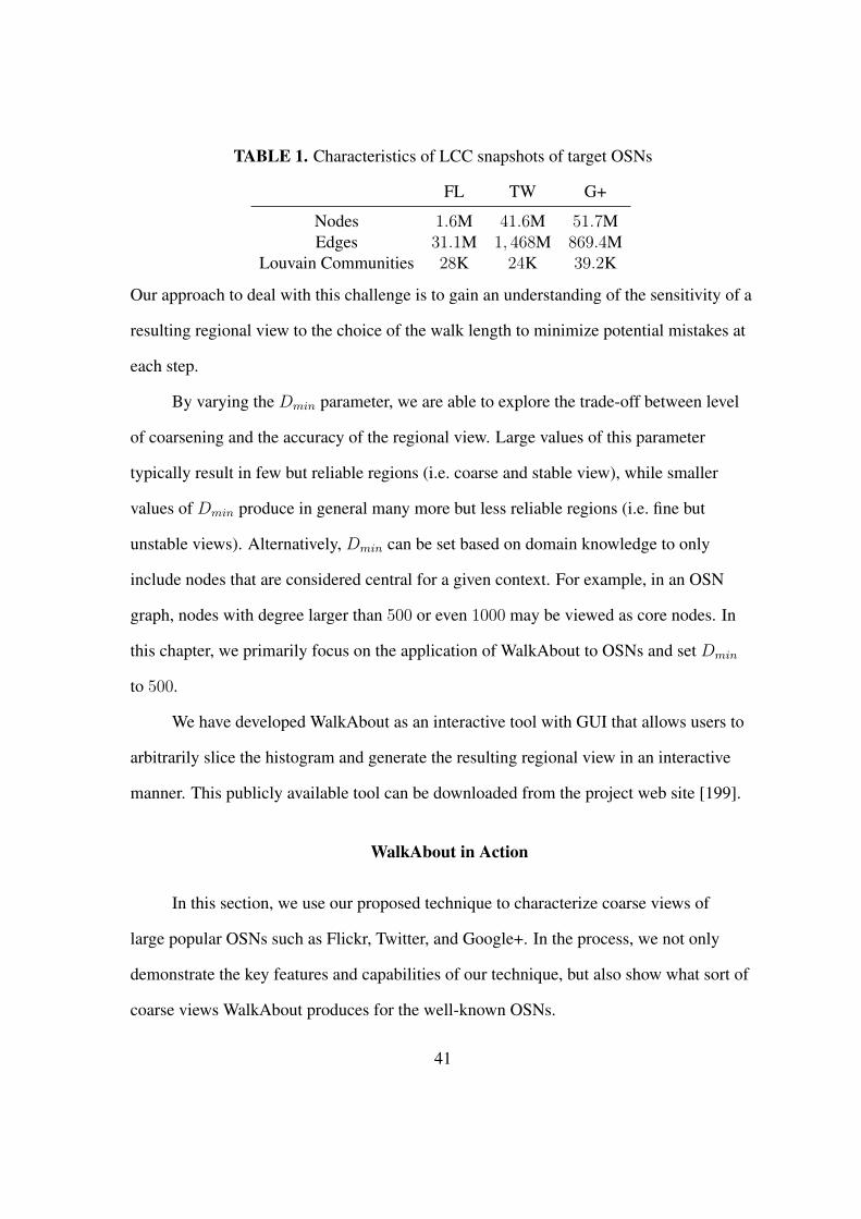
TABLE 1. Characteristics of LCC snapshots of target OSNs
FL TW G+
Nodes 1.6M 41.6M 51.7MEdges 31.1M 1, 468M 869.4M
Louvain Communities 28K 24K 39.2K
Our approach to deal with this challenge is to gain an understanding of the sensitivity of a
resulting regional view to the choice of the walk length to minimize potential mistakes at
each step.
By varying the Dmin parameter, we are able to explore the trade-off between level
of coarsening and the accuracy of the regional view. Large values of this parameter
typically result in few but reliable regions (i.e. coarse and stable view), while smaller
values of Dmin produce in general many more but less reliable regions (i.e. fine but
unstable views). Alternatively, Dmin can be set based on domain knowledge to only
include nodes that are considered central for a given context. For example, in an OSN
graph, nodes with degree larger than 500 or even 1000 may be viewed as core nodes. In
this chapter, we primarily focus on the application of WalkAbout to OSNs and set Dmin
to 500.
We have developed WalkAbout as an interactive tool with GUI that allows users to
arbitrarily slice the histogram and generate the resulting regional view in an interactive
manner. This publicly available tool can be downloaded from the project web site [199].
WalkAbout in Action
In this section, we use our proposed technique to characterize coarse views of
large popular OSNs such as Flickr, Twitter, and Google+. In the process, we not only
demonstrate the key features and capabilities of our technique, but also show what sort of
coarse views WalkAbout produces for the well-known OSNs.
41

Datasets and Methodology
In the following, we rely on anonymized snapshots of the largest connected
component (LCC) of the social graphs of Flickr (FL) that was captured by Mislove et al.
[191], a snapshot of the Twitter (TW) social graph that was collected by Kwak et al.
[163], and a snapshot of Google+ (G+) from a recent study by Gonzalez et al. [119].
Table 1 summarizes the main characteristics of these snapshots.
When applying the WalkAbout technique to each OSN, we consider these snapshots
as undirected graphs, i.e. converting any directed edge between two nodes (for TW and
G+) into an undirected edge, and collapsing a pair of edges if they are reciprocal. For
each OSN, we apply WalkAbout and show the following results: (i) the evolution of the
conditioned dvr histogram (see Section 3.4) as a function of walk length to illustrate
the selection of target walk length. (ii) the shape of the modified histogram at the target
walk length that shows the peaks used for identifying individual regions, (iii) a table that
summarizes the main features of the identified cores (number of nodes and the average
degree in each core) and the corresponding regions (the percentage of total nodes and
edges, average degree and modularity), and (iv) a sketch of the regional view of the OSN.
We refer to the collection of specified values for the WalkAbout parameters, namely
Dmin and wl, as the target setting. In particular, we used Dmin = 500 throughout this
analysis. To examine the robustness of our results to different choices of Dmin values, we
repeated our analysis with Dmin values that are 10% larger or smaller and observed no
significant differences.
42
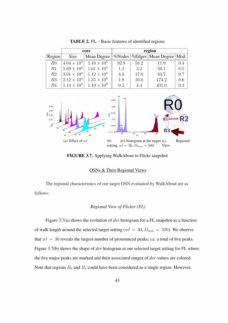
TABLE 2. FL – Basic features of identified regions
core regionRegion Size Mean Degree %Nodes %Edges Mean Degree Mod.R0 4.04× 10³ 1.10× 10³ 92.8 58.2 11.9 0.4R1 5.69× 10² 1.01× 10³ 1.2 3.2 50.1 0.5R2 3.01× 10³ 1.12× 10³ 4.0 17.6 83.7 0.7R3 2.12× 10³ 1.35× 10³ 1.8 16.6 174.2 0.6R4 1.14× 10³ 1.10× 10³ 0.2 4.4 431.0 0.3
15
20
25
30
10
20
30
40
500
0.01
0.02
0.03
0.04
dvrwl
PD
F
(a) Effect of wl
20 25 30 350
0.005
0.01
0.015
0.02
0.025
dvr
PD
F
R0
R1
R2
R3R4
(b) dvr histogram at the targetsetting, wl = 30, Dmin = 500
R0R0R1R1 R2R2
R3R3R4R4
(c) RegionalView
FIGURE 3.7. Applying WalkAbout to Flickr snapshot
OSNs & Their Regional Views
The regional characteristics of our target OSN evaluated by WalkAbout are as
follows:
Regional View of Flicker (FL)
Figure 3.7(a) shows the evolution of dvr histogram for a FL snapshot as a function
of walk length around the selected target setting (wl = 30, Dmin = 500). We observe
that wl = 30 reveals the largest number of pronounced peaks; i.e. a total of five peaks.
Figure 3.7(b) shows the shape of dvr histogram at our selected target setting for FL where
the five major peaks are marked and their associated ranges of dvr-values are colored.
Note that regions R3 and R4 could have been considered as a single region. However,
43

because of the observed dip around dvr = 35, we split that peak into two regions. We
later discuss the effect of this decision. Due to their small sizes and to keep the number
of regions within limits, we did not consider several very small peaks in the middle of the
histogram whose dvr was 21.96 < dvr < 33.4 and contained between 1 to 100 nodes
(with the median of 8 nodes). This is indeed one way to explore the tradeoff between
the accuracy or resolution (by keeping many core components) and complexity of the
resulting view. Note that WalkAbout reveals these peaks and allows us to explore them if
a higher resolution is desired.
Table 2 summarizes the key features of the five identified cores and their
corresponding regions. We observe that the cores include between 500-4000 nodes and
collectively contain less than 1% of nodes of the graph. Except for R1, they are all of
similar sizes. The resulting regions are very imbalanced, with R0 containing more than
92% of all nodes and 58% of all edges and having average degree of 11.9 and modularity
of 0.4. The other regions are very small and contain only some 0.2%-4% of all nodes.
However, regions R2 and R3 have a high average degree and thus include a much larger
fraction of edges. At the same time, regions R2 and R3 have a much higher modularity
than R0. All the identified cores and regions form connected components. Figure 3.7(c)
sketches the regional view of the FL structure. This figure shows that for all practical
purposes, regions R3 and R4 are weakly connected to the other three regions. We recall
that these two regions are created as a result of splitting the right most peak of the dvr
histogram into two parts. Given their strong inter-connectivity, an option would be to
merge these two regions together and consider them as a single region, thus producing a
yet coarser view of the FL connectivity structure.
44
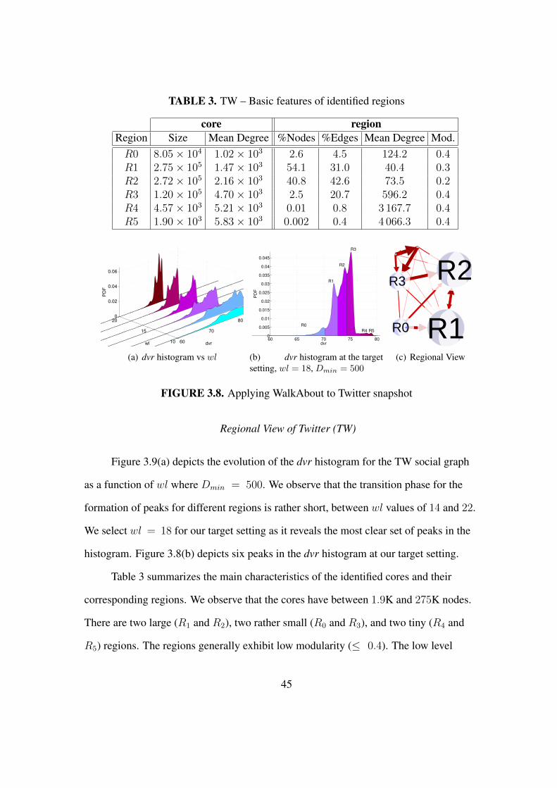
TABLE 3. TW – Basic features of identified regions
core regionRegion Size Mean Degree %Nodes %Edges Mean Degree Mod.R0 8.05× 10⁴ 1.02× 10³ 2.6 4.5 124.2 0.4R1 2.75× 10⁵ 1.47× 10³ 54.1 31.0 40.4 0.3R2 2.72× 10⁵ 2.16× 10³ 40.8 42.6 73.5 0.2R3 1.20× 10⁵ 4.70× 10³ 2.5 20.7 596.2 0.4R4 4.57× 10³ 5.21× 10³ 0.01 0.8 3 167.7 0.4R5 1.90× 10³ 5.83× 10³ 0.002 0.4 4 066.3 0.4
60
70
80
10
15
200
0.02
0.04
0.06
dvrwl
PD
F
(a) dvr histogram vs wl
60 65 70 75 800
0.005
0.01
0.015
0.02
0.025
0.03
0.035
0.04
0.045
dvr
PD
F
R0
R1
R2
R3
R4 R5
(b) dvr histogram at the targetsetting, wl = 18, Dmin = 500
R0R0 R1R1
R2R2R3R3
R4R4
R5R5
(c) Regional View
FIGURE 3.8. Applying WalkAbout to Twitter snapshot
Regional View of Twitter (TW)
Figure 3.9(a) depicts the evolution of the dvr histogram for the TW social graph
as a function of wl where Dmin = 500. We observe that the transition phase for the
formation of peaks for different regions is rather short, between wl values of 14 and 22.
We select wl = 18 for our target setting as it reveals the most clear set of peaks in the
histogram. Figure 3.8(b) depicts six peaks in the dvr histogram at our target setting.
Table 3 summarizes the main characteristics of the identified cores and their
corresponding regions. We observe that the cores have between 1.9K and 275K nodes.
There are two large (R1 and R2), two rather small (R0 and R3), and two tiny (R4 and
R5) regions. The regions generally exhibit low modularity (≤ 0.4). The low level
45

of modularity for regions in TW indicates that regions do not exhibit tight internal
connectivity. An interesting fact about the two tiny regions is that they have an order
of magnitude larger average degree than the other regions but still exhibit the same
modularity. Figure 3.8(c) depicts the resulting regional view for the TW structure and
reveals that regions R1 and R2 have strong mutual connectivity and play a central role
in the graph. R0 is connected to R1 and R2 from one side while R5, R4 and R3 form a
triangle structure that connect to the rest of the regions primarily through R2.
Regional View of Google+ (G+)
Figure 3.9(a) depicts the evolution of the dvr histogram for the G+ graph as we
change wl. The histogram which most clearly reveals different regions is formed around
wl = 20. Therefore, we select this wl as our target setting. The corresponding histogram
is shown in Figure 3.9(b) and reveals the existence of six distinguishable peaks. While the
regions R4 and R5 result from rather small peaks, we still use them as cores because they
are clearly separated from other peaks and also have large average degrees.
TABLE 4. G+ – Basic features of identified regions
core regionRegion Size Mean Degree %Nodes %Edges Mean Degree Mod.R0 2.18× 10⁵ 1.73× 10³ 82.0 62.8 25.8 0.3R1 4.00× 10⁴ 7.13× 10³ 16.3 33.5 69.2 0.6R2 6.51× 10³ 1.70× 10³ 0.6 1.0 54.2 0.7R3 9.94× 10³ 2.28× 10³ 0.9 1.9 73.8 0.8R4 7.40× 101 3.71× 10⁴ 0.2 0.5 74.5 0.7R5 1.45× 10² 1.78× 10⁴ 0.1 0.3 175.4 0.6
Table 4 summarizes the main features of the identified cores and regions. We
observe that the core sizes vary between 74 and 218k which is much more skewed46

20
40
60
80
10
20
30
40
500
0.05
0.1
dvrwl
PD
F
(a) dvr histogram vs wl
20 30 40 50 60 70 800
0.01
0.02
0.03
0.04
0.05
0.06
0.07
0.08
dvr
PD
F
R0
R1
R2R3
R4R5
(b) dvr histogram at the targetsetting, wl = 20, Dmin = 500
R0R0 R1R1R2R2
R3R3
R4R4R5R5
(c) Regional View
FIGURE 3.9. Applying WalkAbout to Google+ snapshot
compared to the other OSNs. These cores lead to a dominant region R0, a moderate-
sized region R1, and four tiny regions. All regions except for R0 exhibit a rather
high modularity (0.6-0.8). Figure 3.9(c) plots the regional view of the connectivity
structure for G+. We observe that R4 and R5 are tightly inter-connected but have a weak
connectivity to the other regions. The other four regions have a moderate chain-like inter-
connectivity structure of the form R2-R3-R1-R0.
Lessons Learned
The obtained regional views of the connectivity structures of some of the most
popular OSNs provide a novel and useful abstraction of the large-scale real-world
systems. They offer a manageable high-order view of how nodes are mapped into various
regions of different sizes, along with a quantitative assessment of the corresponding inter-
and intra-region connectivity.
A common observation from applying WalkAbout to the three OSNs is that separate
regions (peaks) with close-by dvr values tend to have stronger inter-region connectivity
than regions that result from clearly separated peaks in the dvr histogram. Such behavior
is to be expected for real-world graphs. For one, our approach for mapping high degree
47

nodes to cores based on slicing peaks in the histogram is ambiguous for high degree
nodes whose dvr values are close to the border value of a region. Moreover, the size of a
region and its mixing time can vary widely across different regions of a large graph. This
in turn makes the selection of a proper walk length challenging. For example, a particular
walk length that is close to a region’s mixing time and thus clearly reveals the associated
peak in the dvr histogram could be too long for other regions. This behavior can cause
some of the RWs of other regions to leave their starting points and move to other close-by
regions. The fraction of such “misbehaving” RWs depends on the walk length and the
relative connectivity between starting and neighboring regions. Both of the above factors
tend to decrease the gap between the dvr ranges of close-by regions proportional to their
pairwise connectivity. However, given the coarse resolution of the considered regional
views of a graph, the resulting ambiguities do not significantly impact the value that can
be derived from examining such coarse views of large-scale graphs.
Also note that the number of peaks that appear in a dvr histogram changes with
the walk length which, in turn, can change the perspective of what peak size should be
considered to be significant. Our focus here has been on considering only a handful
of regions so that the resulting regional views are manageable. WalkAbout is clearly
an interactive framework and can be used to identify a different number of regions and
examine how such selections affect the characteristics of the resulting regional views.
As our results show, the identified regions by WalkAbout could be very imbalanced
in size. In particular, a large region may consist of two or more smaller regions that are
not properly recognizable during the first round. One way to explore the structure of
these larger regions is to apply WalkAbout to each identified regions. This hierarchical
application might be able to identify the internal structure (sub-regions) of a large region
48

if they have sufficiently distinct average degrees and shorter mixing time than the entire
region. This issue remains as a future work for us to explore in more detail.
The other proposal that is left as future work is to utilize the dvr values computed
at various walk lengths for clustering the vertices in the core. In this schema, each node
will be associated with a vector of dvr values for a range of walk lengths during which the
dvr histograms exhibit separation between peaks. Classic clustering techniques such as
Gaussian Mixture Models or K-means can be used to identify cluster of nodes that have
similar dvr values at different walk lengths, are indeed in areas in the graph with similar
average degree. This approach can be used to (a) identify regions that have different
mixing times, and (b) automate the process of region identification in graph.
WalkAbout as an Interactive Tool
We have implemented WalkAbout as an interactive tool for browsing coarse-view
of connectivity for large graphs. Our tool accepts the edge view of a large graph and
produces dvr histogram. A user can browse through the evolution of the histogram as a
function of the walk length and Dmin to select its desired parameters, and then focus on
the desired histogram to interactively determine the number and location of individual
peaks (regions). Our tool then generates the input for viewing the resulting regional view
on an existing visualization program (such as Gephi [36]). The key feature of our tool is
the ability for a user to interact with the process to determine the proper parameters based
on those interactions. Our tool is publicly available at the project webpage [199].
Regions vs. Communities
Community detection in graphs is a commonly used technique that can also be
viewed as providing a coarse view of a graph (i.e. community-level instead of regional-
49

TW G+ FL0
0.2
0.4
0.6
0.8
Modularity
Louvain
Large Louv
WA
TW G+ FL
101
102
103
Average Degree
TW G+ FL
102
104
106
Size
FIGURE 3.10. Comparison of Louvain communities and WalkAbout regions.
level view). Community detection techniques typically group nodes into tightly connected
groups, called a community, based on an objective function (e.g. modularity) and present
characteristics of the detected communities without emphasis on the inter-community
connectivity. In this section, we compare and contrast the regional view that WalkAbout
produces with the community view of a large graph. Given the similarity between the
notion of a “community” and a “region”, and the popularity of applying community
detection techniques for graph analysis, this comparison helps us relate the regional view
of the graph with a related concept (i.e. community) that is widely used. To this end, we
have to run a community detection technique on our large target graphs. Unfortunately,
most of the commonly-used community detection techniques do not scale to graphs
with more than tens of millions of nodes [84], or require the number of communities
as an input (e.g. Metis [150, 151]), or recursively partition the graph into balanced
communities that may not lead to the most tightly connected communities [150]. Due to
these limitations, we use the Louvain community detection technique [40] that implements
a greedy method to optimize the “modularity” of identified communities. Louvain is often
considered to be the gold standard for scalable community detection and has a publicly
available and robust implementation.
50

We applied Louvain to our targeted OSN structures and identified 28K, 39K,
and 24K communities of various sizes in FL, G+, and TW, respectively. Importantly,
these results show that the number of communities in these graphs are several orders of
magnitude larger than the number of regions. This large number of communities implies
that the graph connectivity at the community level is still too complex for high-level
analysis (e.g. determining the full picture of inter-community connectivity.)
Figure 3.10 presents the summary distribution of the main features (modularity,
size and average degree) across all regions and all communities associated with each each
OSN. It has been shown that community detection techniques such as Louvain tend to
identify a large number of small communities to achieve a high modularity score [169].
To examine the effect of community size, we have also included the results where we
only consider the large communities that consist of 1000 or more nodes. We observe
that communities are typically more than four orders of magnitude smaller than regions.
However, size-wise, the largest communities clearly have an overlap with the obtained
regions. While the modularity of communities is typically higher than the modularity
of regions, this gap is more pronounced in less clustered graphs (e.g. TW) than in more
clustered graphs like FL and G+. Also, the large communities exhibit higher modularity
than the WalkAbout-derived regions, and the average degree of the communities is
smaller than its counterpart for regions (irrespective of community size).
To gain more insight into connectivity-related features, we examine the placement
of the 1000 nodes with the highest degree in each region across the different communities.
Interestingly, we find that in all three OSNs, the top 1000 nodes are located in 5 or 6
communities, with some of those communities attracting significantly more nodes than
others. Moreover, both the size (15K-359K for FL, 72K-22M for TW, and 336K-16M
for G+) and the modularity of these few communities (0.48-0.75 for FL, 0.28-0.78 for
51

TABLE 5. Number of mapped communities to each region
FL
Region CommunitiesR0 26 987R1 173R2 639R3 251R4 7
TW
Region CommunitiesR0 142R1 13 171R2 10 003R3 724R4 9R5 5
G+
Region CommunitiesR0 29 577R1 9 545R2 93R3 32R4 18R5 2
TW, and 0.35-0.89 for G+) are comparable with typical values for the WalkAbout-
derived regions. These results suggest that the large communities that are needed for
accommodating high-degree nodes exhibit characteristics very similar to the WalkAbout-
identified regions.
Mapping Communities to Regions
To further explore the relationship between the community- and regional-level
views of these graphs, we map individual Louvain communities to the identified regions
for the same graph. In particular, for each community c, we determine the region where
each node of this community is located and identify the region R that contains a majority
of nodes in that community. Then community c is mapped to that region R that hosts
a majority of its nodes, and the confidence for this mapping is equal to the fraction of
c’s nodes that are located in R. Table 5 summarizes the number of communities that are
mapped to the individual regions of each OSN. In the extreme case, if the nodes in each
community are randomly located in different regions, then all communities are mapped to
the largest region(s) with a confidence equal to the region’s relative size. We observe that
the mapping confidence for 75% of the communities in every single region is 100%, and
for 90% of communities, all but one small region in FL (R4) has a mapping confidence
52
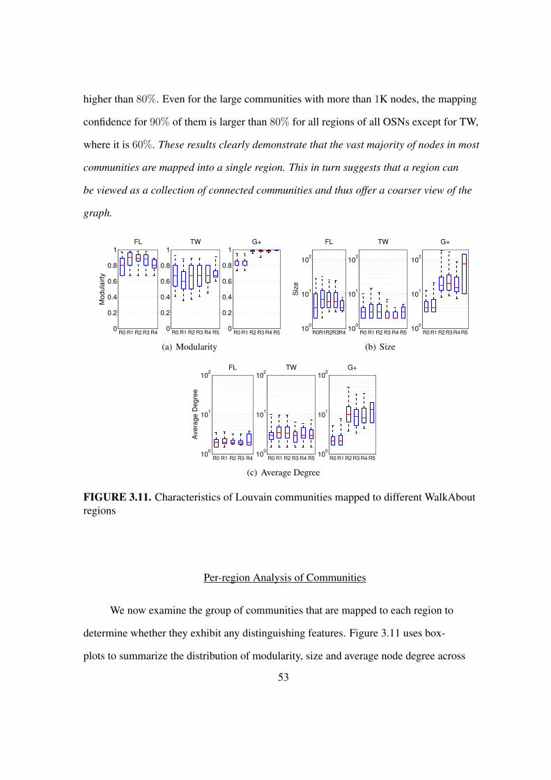
higher than 80%. Even for the large communities with more than 1K nodes, the mapping
confidence for 90% of them is larger than 80% for all regions of all OSNs except for TW,
where it is 60%. These results clearly demonstrate that the vast majority of nodes in most
communities are mapped into a single region. This in turn suggests that a region can
be viewed as a collection of connected communities and thus offer a coarser view of the
graph.
0
0.2
0.4
0.6
0.8
1FL
R0 R1 R2 R3 R4
Mo
du
lairty
0
0.2
0.4
0.6
0.8
1TW
R0 R1 R2 R3 R4 R50
0.2
0.4
0.6
0.8
1G+
R0 R1 R2 R3 R4 R5
(a) Modularity
100
101
102
FL
R0R1R2R3R4
Siz
e
100
101
102
TW
R0 R1 R2 R3 R4 R510
0
101
102
G+
R0 R1 R2 R3 R4 R5
(b) Size
100
101
102
FL
R0 R1 R2 R3 R4
Ave
rag
e D
eg
ree
100
101
102
TW
R0 R1 R2 R3 R4 R510
0
101
102
G+
R0 R1 R2 R3 R4 R5
(c) Average Degree
FIGURE 3.11. Characteristics of Louvain communities mapped to different WalkAboutregions
Per-region Analysis of Communities
We now examine the group of communities that are mapped to each region to
determine whether they exhibit any distinguishing features. Figure 3.11 uses box-
plots to summarize the distribution of modularity, size and average node degree across
53

102
104
105
G+
TW
FL
Second
Louvain
WA: Map to Core
WA: dvr
FIGURE 3.12. The comparison of the execution time for different techniques.
all communities that are mapped to each region of individual OSNs. These figures
illustrate that there does not appear to be a strong correlation between the modularity
of communities in a region and the modularity of the entire region. This observation is
explained by the fact that the modularity of a region depends, among other factors, on
the inter-community connectivity. We also observe that in general, there is no significant
difference in the modularity, size and average degree of the communities that are mapped
to each region, i.e. regions are not generally distinguishable based on the characteristics
of their communities despite the difference in their average degree and size. The only
exceptions to this observation are regions R3, R4 and R5 in G+ that contain communities
with a significantly higher and more homogeneous modularity, larger size and higher
average degree. This is intriguing since larger size or higher node degree could lead
to lower modularity in a single community. These findings suggest that identifying
individual regions by merging communities in a bottom-up fashion (using modularity)
is in general challenging. Alternatively, a top-down approach to region detection such as
WalkAbout shows more promise.
54

Comparing Run-time
Finally, we compare the run times of WalkAbout and the Louvain community
detection technique on an Intel X5650 2.66GHz computer with 72GB RAM which is
sufficient to hold the entire social graph of any target OSN in memory. Figure 3.12 shows
the comparison of the run time per individual technique over each OSN using log scale
for the x-axis. We further split the run time of WalkAbout into two components: (i) the
calculation of the dvr values for high degree nodes to detect cores and (ii) mapping of
low-degree nodes to those cores. These results show that the run times of both techniques
are similar over small graphs (e.g. 10 second difference for FL). However, as the graph
size increases, Louvain requires a significantly longer run time and the gap between
WalkAbout and Louvain seems to be widening. We also recall that for graphs of the
size of these OSNs, many popular community detection or graph clustering techniques
(including spectral clustering [72]) quickly run into scalability issues and cannot be used
at all [107].
A New Kind of Validation
So far we have primarily focused on the connectivity features of regions and
how they are aligned with smaller entities in a large graph such as communities. Since
regions are not derived based on an objective function, there is no obvious way to
validate/examine their accuracy. To tackle the challenging problem of “validation” of
WalkAbout-derived regions, we conduct a case study to investigate whether users in each
identified region exhibit similar social attributes that act as the underlying factors for the
formation of the region.
55

0
0.2
0.4
0.6
0.8
1
Gro
up
Ma
pp
ing
Co
nfid
en
ce
R0 R1 R2 R3 R4
(a) FL – 99K groups
0
0.2
0.4
0.6
0.8
1
Gro
up
Ma
pp
ing
Co
nfid
en
ce
R0 R1 R2 R3 R4
(b) FL – 44K large groups
FIGURE 3.13. Distribution of confidence in mapping groups to identified regions. Largegroups have more than 10 members.
Are Regions Meaningful?
Our ability to answer the posed question depends on the availability of
semantically-rich metadata that contains social context. However, given adequate
metadata, answering the above question will shed light on whether an identified region
represents a meaningful portion of an OSN. In our case study, we focus on FL because of
the availability of rich metadata with social context for this OSN.
More precisely, for our FL snapshot, we have a list of 99K social groups (with
their names) where each group consists of a collection of users with common interest.
A user can be a member of multiple groups. The names of most groups provide great deal
of information about the groups’ interests or context (e.g. big and hot, bigblkmuscles,
bigbulls, boys, everydaymen, fatboys). Similarly to the mapping of communities
to regions (Section 3.6), we map each group to a region where most of their users
are located. Figure 3.13(a) and 3.13(b) shows the summary distribution of mapping
confidence for all groups and for the 44K groups with more than 10 users to the five
regions in FL, respectively. We observe that groups that are mapped to regions R1-R4
exhibit a very high confidence despite the small size of these regions. The mapping
confidence drops for larger groups but it is still a couple of orders of magnitude larger
56

than the relative size of the group. More specifically, regions R1, R2, R3 and R4 make
up 1.2%, 4%, 1.8%, and 0.2% of nodes in the graph but the typical confidence for their
mapped groups is 0.8, 0.9, 0.92, and 0.58, respectively. These results suggest that the
social context of each group is likely a driving force for its mapping to these four regions.
In contrast, the typical confidence for mapped groups to region R0 is comparable to
its relative size. This indicates that social forces discernible from our data may not be
primarily responsible for the mapping of groups to region R0. To learn the context of
individual regions, we manually examined the names of groups that are mapped to
that region. Our examination reveals a very pronounced pattern among group names
associated with the following regions2: Group names in R1 are mostly related to male
nudity and adult content, group names in R2 are hinting at female nudity and adult
content, and group names in both R3 and R4 have a common ethnic attribute, i.e. either
have Arabic names or posts in Arabic, which is aligned the finding is Section 3.5 that
positions the two regions in close proximity of each other. As expected, group names in
R0 do not show a coherent theme.
Are Communities Meaningful?
We use the same methodology to examine the “validity” of communities;
i.e. checking whether the names of mapped groups to individual communities indicate
a common social theme in the community. In the case of regions without any pronounced
social theme (e.g. R0), one of their large communities may indeed have a social context
whereas for regions with an existing social context (e.g. R1), a community may offer an
even more specific context. The large number and diverse size of communities in the FL
2The spreadsheet of FL group names that are mapped to each FL regions (or community) are availableonline at http://onrg.cs.uoregon.edu/WalkAbout/group_per_region/
57

social graph make it difficult to examine all communities. Since small communities do
not provide sufficient information to identify their social theme, we only focus on the
three largest communities that are mapped to each region of FL. Careful examination
of names of groups that are mapped to each one of these large communities reveals that
large communities in R0 do not seem to have any social theme and large communities in
all other regions often exhibit a theme that is very similar to the identified theme for the
whole region. The only exception is a community in R2 that contains groups with clearly
more specific group names. In summary, our preliminary investigations suggest that some
large communities that are embedded within a region are not “meaningful” in the sense
that they exhibit rather diverse social themes that makes them not much more focused
than the WalkAbout-identified region in which that they reside.
Summary
In this chapter, we present a new scalable framework called WalkAbout for
examining and inferring regional views of connectivity for very large graph and
demonstrate its application to three well-known OSNs. Moreover, we conduct a
comparison between regional- and community-level views of large OSN and present a
case study where we “validate” the individual regions and communities; i.e. examining
in detail the available meta-data for social themes that are associated with the obtained
groupings of nodes in an OSN and are prime candidates for the root cause(s) behind the
formation of these groupings.
The presented design of WalkAbout and the experience we gained from applying it
to real-world OSNs suggest a number of extensions and improvements. We are currently
exploring the usage of different walk lengths for computing a dvr vector, as opposed
to a single dvr value, that could result in identification of region cores at different
58

random walk lengths. We also plan to explore the recursive application of WalkAbout
to identify potential sub-regions within each identified region. In the same vein, we
intend to examine how the regional- and community-level views of a large graph can
inform each other to yield a hybrid approach for a “multi-scale” exploration of the graph’s
connectivity (e.g. examining the connectivity between large communities within a given
region to obtain a higher-resolution view of graph connectivity). Extending WalkAbout to
allow for overlapping regions by dealing region core as landmarks in the graph is another
line of future research. Finally, collecting semantically rich meta-data that enables the
illustrated validations of groupings such as regions, clusters, or communities is another
item on our research agenda in this area.
59

CHAPTER IV
CHARACTERIZING AND COMPARING GROUP-LEVEL USER BEHAVIOR IN
MAJOR ONLINE SOCIAL NETWORKS
The research conducted on the characterization of Online Social Networks in the
last years has created a solid basis to address fundamental, yet challenging issues such as
identifying the most suitable OSN for different purposes (e.g. broadcasting information
or obtaining feedback) and defining initial guidelines for an informed utilization of
OSNs. What is necessary to address many of these issues is a quantitative comparison
between the behavior of users in different OSNs. The challenge is, however, the large
size of these networks, which renders such a comparison not trivial. On the other hand
the user properties and behavioral attributes are reported to be skewed which further
complicates this comparison. In this chapter, we propose a new methodology for a
detailed measurement study to characterize and compare the behavior OSNs at the
“group-level”. Based on this methodology, we conduct a comparative analysis on the
behavior of users in Facebook (FB), Twitter (TW) and Google+ (G+). We focus on
Popular, Cross (with account in three OSNs) and Random groups of users in each OSN
since they offer complementary views. We capture user behavior with the following
metrics: user connectivity, user activity and user reactions. Our group-level methodology
enables us to capture major trends in the behavior of small but important groups of
users, and to conduct inter- and intra-OSN comparison of user behavior. Furthermore,
we conduct temporal analysis on different aspects of user behavior for all groups over
a two-year period. Our analysis leads to a set of useful insights including: (i) Popular
Facebook users have 4 and 47 times more followers than Popular Twitter and Google+
users, respectively. (ii) The more likely reaction by Facebook and Google+ users is to
60

express their opinion whereas Twitter users tend to relay a received post to other users
and thus facilitate its propagation. Despite the culture of reshare among Twitter users, a
post by a Popular Facebook user receives more Reshares than a post by a Popular Twitter
user. (iii) Added features in an OSN can significantly boost the rate of action and reaction
among its users.
Introduction
Major Online Social Networks (OSNs) such as Facebook or Twitter are among
the most popular services on the Internet with billions of subscribers and hundreds
of millions of daily visitors. OSNs enable individual users to connect to other users,
disseminate their information throughout the network while collecting the reactions
from other users without any geographic or time constraint. These unique capabilities
have motivated different entities, ranging from individuals and celebrities to companies
and sport teams to join OSNs often with different goals. For isntance, OSNs enable
individual companies to closely interact with their customers and receive feedback on
their products [42]. The growing popularity of major OSNs has effectively turned them
into “online societies” with a profound impact on the social, political and economical
aspects of our daily lives.
The growing importance of large OSNs raises a basic question: How do users
behave with respect to publishing posts and reacting to other users’ posts in a specific
OSN? Shedding any light on these seemingly simple questions not only informs current
users of an OSN that to what extent an OSN might serve their goals but also enables
non-member entities to assess whether the OSN might be a fit for their needs. To
underscore the importance of these issues, it is worth noting that many companies pay
large premiums in order to adopt various techniques that may help them attract a larger
61

number of active followers in a major OSN. However, tackling the above questions is
challenging for several reasons including the following: First, users in an OSN often
exhibit a diverse characteristics with skewed distributions [97]. Identifying interesting
groups could be difficult specially if there is not a reliable way of identifying their
users. Second, existing theories and techniques in “behavioral sciences” are not easily
applicable to OSNs in large scale because they often require the collection of specific data
through customized questionnaires which is not feasible for large scale data collection
over OSNs. Third, even characterizing the behavior of individual users based on their
basic attributes (e.g. connectivity, posted content and their reactions) could be complex
due to the difficulties in determining user intentions (for establishing a connection, or
generating a post, or reacting to other users’ posts). Fourth, in the absence of a uniform
methodology to characterize user behavior across multiple OSNs, it is not feasible to
meaningfully compare and contrast them. In the face of these challenges, a large body
of prior empirical research on OSNs has often focused on specific characteristics of a
single OSN such as user connectivity [119, 163, 117], evolution of OSN size [217] or user
behavior [127, 275].
In this chapter, we characterize and compare the behavior of users in three major
OSNs, namely Facebook (FB), Twitter (TW) and Google+ (G+). The first contribution
of this study is our methodology which relies on “group-level” data collection,
characterization and comparison. We focus on the following three interesting groups
of users in each OSN as follows: Popular users with a very large number of followers,
Cross users with verified accounts in all three OSNs, and Random users. Popular users
represent the most well-connected entities in each OSN while Cross users are entities with
common interest in all three OSNs and Random users show the behavior of the crowd (i.e.
many low-degree, moderately active users). Our approach to characterize user behavior
62

at the group-level has several advantages: (i) It allows us to cope with the diversity of
user behavior which is expected to be much more homogeneous within each group, (ii) it
naturally lends itself to sampling as we need to focus on sample users in selected groups,
(iii) we can meaningfully compare the behavior of similar groups in different OSNs, and
(iv) comparing the behavior of different groups in a single OSN often offers a valuable
insight. We rely on three set of metrics to characterize the behavior of a user in each
group: the connectivity of the user in the social graph, the activity of the user with respect
to publishing posts, and the reaction of other users (e.g. likes and comments) to the user’s
posts.
The second contribution of this study is a detailed measurement that presents a
head-to-head comparison between FB, TW and G+. We carefully populate the three target
groups in each OSN, collect their information using custom crawlers and characterize
the group-level behavior using our three sets of metrics as we present in Section 4.2.
In particular, users in the Cross group allow us to view and compare the ecosystem of
these three OSNs from the perspective of the same set of users. Using the collected
information for users in target groups, we conduct group-level characteristics of users by
examining different aspects of their connectivity (in Section 4.4), activity (in Section 4.5)
and received reactions to their posts (in Section 4.6). We also conduct temporal analysis
on the daily rates of actions and reactions for each groups in different OSNs in Section
4.8. Our analysis leads to a series of inter- and intra-OSN comparison between groups
that reveal to the following important insights:
(i) TW is the OSN that observes a higher volume of information (i.e. posts). However,
despite the lower volume of posts, FB presents a higher volume of reactions. G+ is
currently far behind both FB and TW in both the volume of activities and reactions,
63

except in the case of Popular G+ users that exhibit a similar level of activity to Popular
FB users.
(ii) Our results indicate that TW users prefer to broadcast (i.e. Retweet) information
posted by their friends whereas in G+ users prefer to provide feedback (in the form
of Comments or Likes). FB users also show a preference toward feedback reactions,
however the number of Reshares per post is equal in FB and TW.
(iii) The level of popularity among Popular users in major OSNs seems to be dictated
by external factors and is not influenced by the level of activity of users in the OSN.
However, popularity is correlated with both level of activity and reactions among
unpopular users.
(iv) Posts including photos and videos are more attractive compared to posts including a
link or text only posts. However, videos are still one of the least common types of posts
representing less than 11% of all posts.
The previous observations help to shed a light on some of the initial questions. In
particular, we conclude that:
(i) TW seems to be the most suitable OSN for users interested in consuming information
(i.e. readers) due to the higher volume of information in that OSN. Furthermore, TW or
FB would be the more appropriate OSN for those users interested on propagating their
information (e.g. advertisement campaigns), and FB and G+ are also a great fits for users
interested in obtaining feedback (e.g. from voters or fans).
(ii) Popular users do not need to be very active in major OSNs to increase their popularity.
Instead, users interested in attracting more reactions should focus on publishing photos
and videos.
64

Methodology & Datasets
Characterizing user behavior is challenging because user attributes often exhibit a
very skewed distribution in major OSNs. Therefore, any characterization of the overall
user population in an OSN would primarily represent a significant number of users with
a low level of connectivity to the rest of social graph andmoderately active users. Clearly
such characterization does not reveal much about other important group of users (e.g.
users with a large number of followers) if they only compose a very small fraction of total
user population. Furthermore, the characteristics of individual users in a specific group
may also significantly vary. To cope with these issues, we conduct our analysis at the
group-level rather than user-level since the collective characteristics of users in a group
offer a more reliable measure of their behavior. We consider the following three groups of
users that intuitively represent complementary subsets of user population in each OSN:
– Random users provide a global view of user population that primarily represents a
large fraction of typical users with moderate to low connectivity and activity (i.e.
the crowd).
– Popular users attract the largest number of followers in an OSN and thus represent
the most visible (i.e. well connected) accounts in an OSN.
– Cross users represent samples of users that have an account in all three target
OSNs. Having a concurrent footprint in all three OSNs suggests the particular
interest among these users and a special role that they might play in the overall
ecosystem of major OSNs.
Considering these three groups in each OSN enables us to conduct meaningful
comparisons between different groups within each OSN or similar groups across different
65

OSNs without the need for capturing a complete snapshot of individual OSN which is
not often feasible. While we generally refer to an account in each OSN as a “user”, each
account can clearly represent many other entities ranging from celebrities and politicians
to companies and sport teams. Next we briefly describe our techniques for populating the
dataset of each group.
Random Users
Given various constraints for data collection from each OSN, we need to use a
different approach to select random users in each OSN: For G+, we have collected a
snapshot of the largest connected component (LCC) of the network and selected a random
subset of LCC users. FB offers two types of accounts: (i) regular accounts and fan pages.
Regular accounts are created by individual users and their number of friends is limited to
only 5K1. Fan pages, however, are created by individuals, groups and companies in order
to broadcast information to their fans as they do not have any limitation on the number of
followers. In order to properly compare inter- and intra-OSN comparison between groups,
we only focus on random fan pages (or pages) in FB. FB provides an indexed list of all
the fan pages2, that allows us to easily identify a random subset of these users. Finally,
we select random TW users by examining random IDs that are associated with valid users
[217]. Toward this end, we monitor TW’s public timeline to detect some of the newly
generated accounts and use a conservative estimate for the valid range of ID space.
1We recall that connections between FB users are bidirectional. Thus, the number of followers andfriends for each users is the same.
2https://www.facebook.com/directory/pages
66

Popular Users
This group includes accounts with a very large number of followers (i.e. popular
users). In G+, we have selected accounts from the LCC with the largest number of
followers. Since capturing complete snapshots of TW and FB are not feasible due to their
large size and the limitations imposed by their APIs, we have relied on external sources3
to obtain sorted lists of 20K most popular users. We have crawled the reported 20K most
popular users in each OSN to collect their up-to-date number of followers and determine
their proper ranking within the list of most followed accounts. Our approach to identify
popular users is reasonable since (i) very popular users in major OSNs are often well-
known in the marketing and social-media communities, and (ii) potentially missing few
popular users from this group should not qualitatively affect our analysis.
Cross Users
Identifying users that have an account in all three OSNs is a non-trivial task. To
achieve this goal, we leverage the explicit links that G+ users provide to their FB and TW
accounts in their profiles. We examined all G+ users inside its LCC and identified all G+
users with explicit links to their TW and FB accounts. We filtered users who provided
more than one links to another OSN4 and identified 7.3K G+ accounts with exactly one
link to FB and TW. We have manually inspected some of these “triplet accounts” and
confirmed that they are associated with the same individual user or company in all cases.
3www.socialbakers.com,www.alianzo.com,www.twitaholic.com
4Our closer inspection revealed that some of these users improperly set these links, e.g. listing links totheir favorite accounts in another OSN.
67

While we have a large number of random and popular accounts from all three
OSNs, we limited the number of users in all groups to 7.3K (i.e. the size of the Cross
group) in order to ensure a proper comparison.
Collected Information
We have developed a separate crawler for each OSN that uses its API features to
collect the following information for the selected users in each group:
– User Profile: The profile provides the number of followers and friends and (in some
OSNs) the creation otime of user account. If account creation time is not explicitly
specified in the profile, we use the time of first user post as a good estimate for its
creation time.
– Account’s Activity: In this study, all the public posts (or tweets) generated by the
user along with their timestamps make up its activity. This information enables
us to classify collected posts based on their content into five categories: “text”,
“video”, “photo”, “link” and “other”5. Examples of “other” post types are check-
in in FB and Hangout in G+. One limitation in collecting account activity is that
the TW API only provides the last 3 200 tweets for each user. This implies that the
captured tweet history for very active TW users could represent a limited recent
window of time in case the user published more than 3.2K tweets. We discuss
the implications of this limitation on our analysis in Section 4.8. Throughout this
chapter we use the terms post and tweet interchangeably.
– Reactions to Posts: For any captured public post, we also collect all the following
types of public reaction to the post: (i) Likes (in FB), +1s (in G+) and Favorites (in
5Twitter only supported “text” and “link” type of posts at the time of this study.
68

TW) are reactions by other users who indicate their interest to a post; (ii) Shares
(in FB), Reshares (in G+) and Retweets (in TW) are reactions by which a user
relays a received post to her followers; (iii) Comments on a post are (positive or
negative) reactions by other users. Note that the support for retrieving comment
reactions did not exist in the TW API at the time of our data collection. For clarity
of discussion in the rest of this chapter, we will refer to these types of reactions as
Likes, Reshares and Comments, respectively.
Crawlers
Further details about our crawlers and their performance is as follows.
Facebook crawler: This crawler receives a user ID (or username) as input and uses
the FB API to collect the number of fans, the posts as well as all the reactions to
each individual post of that user. Furthermore, the crawler allows the gathering of
more detailed information such as the type of post. To gain access to posts (and other
information) the FB API requires the use of a valid access token that is provided to
registered FB applications. In addition, FB imposes a maximum number of 600 queries
in the period of 10 minutes. In order to speed up our crawling process we use multiple
instances of the crawler working in parallel.
Twitter crawler: Our TW crawler receives as input a user identifier that can be either
a TW id or screen-name and queries the TW API to obtain the user’s profile attributes,
the total number of published tweets, and the most recent 3 200 tweets published by the
user along with the number of reactions associated with each one of the user’s tweets.
Consequentially if a user has published more than 3 200 tweets, we can only retrieve the
last 3 200. At the time of this study, TW imposed a limit of 150 requests per hour per IP
address. To overcome this limitation, we used PlanetLab [71] infrastructure to parallelize
69

our data collection process. Specifically, our crawler sends requests to TW API using
approximately 450 PlanetLab machines as proxies6, so that we can multiply the speed of
our data collection in proportion to the number of used proxies.
G+ crawler: This crawler is composed by two modules. The first one collects the public
profile information as well as the connectivity information of all the users in the largest
connected component (LCC) of G+. This module is a web-crawler that parses the web
page of G+ users to collect the previous information. The second module uses the G+
API to collect all the public posts as well as their associated reactions. Google limits the
number of queries to the G+ API to 10K per hour per access token. In order to overcome
the rate limit we have created several hundred accounts with their correspondent access
tokens and leverage the proxies infrastructure in PlanetLab explained above to speed up
our crawling data collection. Further details on this crawler can be found in [119].
We re-emphasize that our crawlers only collect publicly available information.
Prior studies have reported that 92-94% of Twitter accounts are public [217, 59] whereas
roughly 33% of posts in G+ are public [148]. Furthermore, all the posts published by FB
pages are public by definition.
TABLE 6. The duration of data collection for different target OSNs
OSN Start date Duration
FB 3/12/2013 9 daysTW 4/28/2013 5 daysG+ 5/27/2013 1 days
Table 6 lists the start time and duration of crawl for each dataset. Table 7
summarizes the basic information for the datasets associated with our three target groups
in each OSN as follows: (i) the aggregate number of posts (and some other attributes)
6Note that the proxy functionality is not native in PlanetLab nodes, so we have installed these proxies inPlanetLab nodes.
70
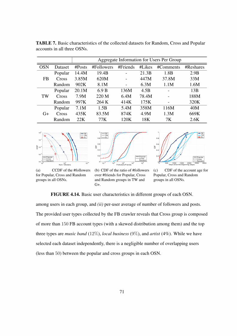
TABLE 7. Basic characteristics of the collected datasets for Random, Cross and Popularaccounts in all three OSNs.
Aggregate Information for Users Per Group
OSN Dataset #Posts #Followers #Friends #Likes #Comments #Reshares
FBPopular 14.4M 19.4B - 21.3B 1.8B 2.9BCross 3.85M 620M - 447M 37.8M 33M
Random 902K 8.1M - 6.3M 1.1M 1.6M
TWPopular 20.1M 6.9 B 136M 4.5B - 13BCross 7.9M 220 M 6.4M 78.4M - 188M
Random 997K 264 K 414K 175K - 320K
G+Popular 7.1M 1.5B 5.4M 358M 116M 40MCross 435K 83.5M 874K 4.9M 1.3M 669K
Random 22K 77K 120K 18K 7K 2.6K
100
105
1010
10−4
10−3
10−2
10−1
100
Num. followers
CC
DF
FB
TW
G+
Popular
Cross
Random
(a) CCDF of the #followersfor Popular, Cross and Randomgroups in all OSNs.
10−2
100
102
104
106
0
0.2
0.4
0.6
0.8
1
Followers/Friends
CD
F
FB
TW
G+
Popular
Cross
Random
(b) CDF of the ratio of #followersover #friends for Popular, Crossand Random groups in TW andG+.
0 500 1000 1500 2000 2500 30000
0.2
0.4
0.6
0.8
1
Days since the beginning (days)
CD
F
FB
TW
G+
Popular
Cross
Random
(c) CDF of the account age forPopular, Cross and Randomgroups in all OSNs.
FIGURE 4.14. Basic user characteristics in different groups of each OSN.
among users in each group, and (ii) per-user average of number of followers and posts.
The provided user types collected by the FB crawler reveals that Cross group is composed
of more than 150 FB account types (with a skewed distribution among them) and the top
three types are music band (12%), local business (9%), and artist (4%). While we have
selected each dataset independently, there is a negligible number of overlapping users
(less than 50) between the popular and cross groups in each OSN.
71

Connectivity & Account Age
In this section, we briefly examine the connectivity of individual users and their
account age. These basic characteristics of target groups not only provide useful context
for the rest of our analysis but can also be viewed as a part of group-level behavior. Figure
4.14(a) depicts the CCDF of the number of followers for users in each target group using
a log-log scale. Groups associated with each OSN are shown with a different colors using
a different line type for each group. Figure 4.14(a) demonstrates that the distribution of
number of followers (i.e. out-degree) among users in each group is much less skewed than
the entire user population as it was reported in prior studies (e.g. [257, 29, 163, 119]).
Furthermore, Popular users in all OSNs exhibit a larger variations in their number of
followers (out-degree of the nodes in the social graph). We observe a clear separation
in the popularity of groups in different OSNs where FB is the most and G+ is the least
popular among similar groups. For instance, the median number of followers among
Popular FB, TW, and G+ users are 1.92M, 490K and 41K, respectively. Figure 4.14(b)
presents a complementary aspect of user connectivity by depicting the CDF of the ratio
of #followers to #friends for individual users in TW and G+ groups. This figure clearly
illustrates that the connectivity of Popular users is very imbalanced as they have thousand
times more followers. The connectivity of Cross users is relatively more balanced as
this group contains users with more followers and also users with more friends. The
Random group also has a relatively balanced connectivity but its fraction of users with
more friends is larger than Cross group.
Figure 4.14(c) shows the CDF of account age (i.e. the time between the account
creation and our data collection time7) for users in each group. We observe that accounts
7Since FB and G+ do not explicitly provide the account creation time, we estimate it using the time ofthe first post.
72

in TW groups are rather older than FB and much older than groups in G+. Interestingly,
the relative age of accounts among three groups in each OSN is similar, with Random
accounts are generally older and Popular accounts are generally younger than other
groups.
Popular Cross Random10
−3
10−2
10−1
100
101
102
Po
st
Ra
te (
po
sts
/da
y)
FB
FB
FB
TW
TW
TW
G+
G+
G+
FB
TW
G+
FIGURE 4.15. CDF of averagenumber of daily posts per user
0 0.2 0.4 0.6 0.8 10
0.2
0.4
0.6
0.8
1
% of users
Accum
ula
tive %
of posts
FB
TW
G+
Popular
Cross
Random
FIGURE 4.16. Skewness ofposts/tweets contributions
User Activity
This section focuses on the group-level analysis of user activity in the three OSNs
from a few different angles. By “activity”, we refer to an action of a user that leads to the
created of a post (or tweet). The published post can be original or a reshare of another
user’s post.
Average Activity Rate
We use the average post rate of a user in terms of the number of posts per day as
the primary indicator of her level of activity which is independent of her account age.
Figure 4.15 shows the summary distribution of activity rate among users in each target
group for all three OSNs using the boxplot format (representing 5th, 25th, 50th, 75th and
73

95th percentiles) with log scale y axis. This figure reveals the following interesting points:
First, within each OSN, the relative order for user activity from high to low is Popular,
Cross and Random group. This relative ordering is more pronounced in TW and G+.
The activity rate within each group often varies around two orders of magnitude. The
skewness in the distribution of activity rate in all groups varies among different groups
(as shown in Figure 4.16). In Popular groups as well as Cross groups in FB, the top 20%
of users generate roughly 66% of daily posts. However, the top 20% of users in the cross
groups in TW and G+ and random group in FB are responsible for 80%-90% of all posts
in their group. The contribution of users in random G+ and TW is the most skewed with
5% of users being responsible for 90% of the posts. Second, comparing the activity rate of
popular users across three OSNs indicates that popular FB and G+ users exhibit a rather
similar rate (with respect to the median and the range of values) which is roughly an order
of magnitude lower than popular TW users. Third, the activity rate of cross users on TW
is the highest (with the median value of 1 post/day) which is followed by their posting
rate on FB (with the median value of 1 post every 2.5 days). These users post on their G+
accounts at a much lower rate of once a month. Fourth, among the Random groups, FB is
the most active one and is followed by TW and then G+. Specifically, a typical FB, TW
and G+ user publishes 0.07 posts/day, 0.02 posts/day, and 0.01 posts/day, respectively.
Random TW users show a significantly larger variation in their activity rate compared to
user in other Random groups.
Abandoned Accounts
The average activity rate of a user only offers a coarse measure of the overall rate
at which a user publishes posts over the age of her account. More specifically, the activity
rate does not directly indicate whether a user regularly visits her account to publish post
74
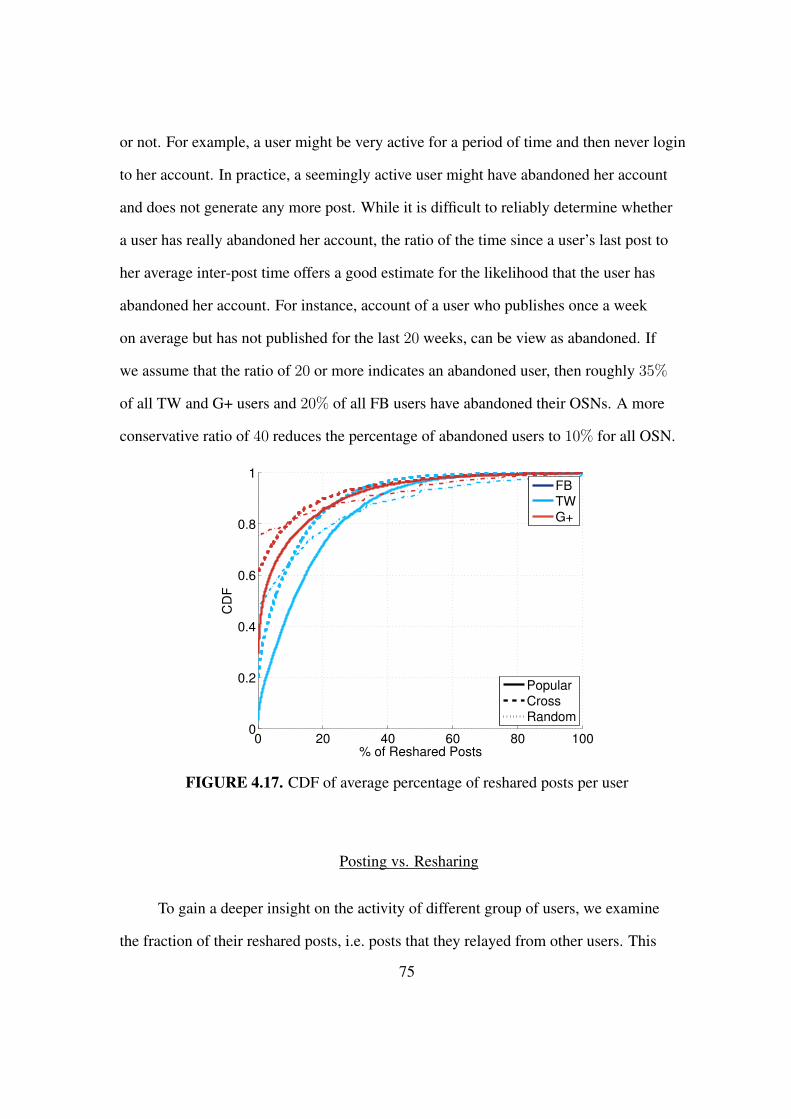
or not. For example, a user might be very active for a period of time and then never login
to her account. In practice, a seemingly active user might have abandoned her account
and does not generate any more post. While it is difficult to reliably determine whether
a user has really abandoned her account, the ratio of the time since a user’s last post to
her average inter-post time offers a good estimate for the likelihood that the user has
abandoned her account. For instance, account of a user who publishes once a week
on average but has not published for the last 20 weeks, can be view as abandoned. If
we assume that the ratio of 20 or more indicates an abandoned user, then roughly 35%
of all TW and G+ users and 20% of all FB users have abandoned their OSNs. A more
conservative ratio of 40 reduces the percentage of abandoned users to 10% for all OSN.
0 20 40 60 80 1000
0.2
0.4
0.6
0.8
1
% of Reshared Posts
CD
F
FB
TW
G+
Popular
Cross
Random
FIGURE 4.17. CDF of average percentage of reshared posts per user
Posting vs. Resharing
To gain a deeper insight on the activity of different group of users, we examine
the fraction of their reshared posts, i.e. posts that they relayed from other users. This
75
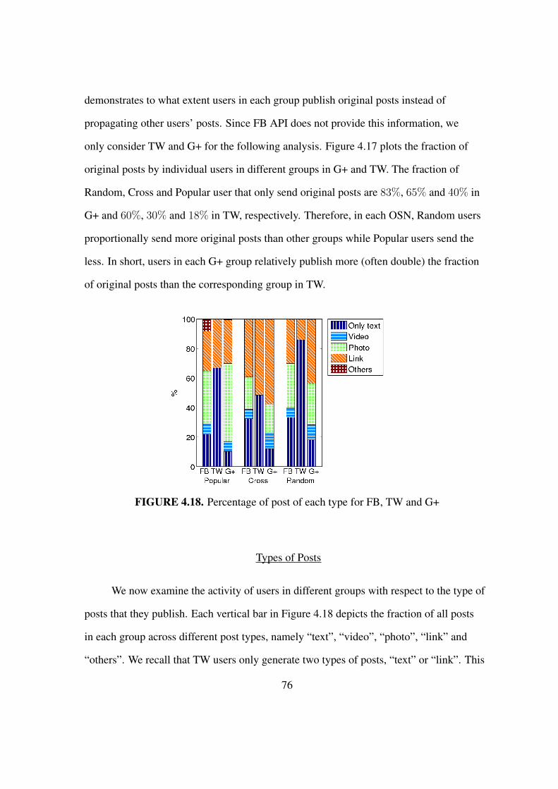
demonstrates to what extent users in each group publish original posts instead of
propagating other users’ posts. Since FB API does not provide this information, we
only consider TW and G+ for the following analysis. Figure 4.17 plots the fraction of
original posts by individual users in different groups in G+ and TW. The fraction of
Random, Cross and Popular user that only send original posts are 83%, 65% and 40% in
G+ and 60%, 30% and 18% in TW, respectively. Therefore, in each OSN, Random users
proportionally send more original posts than other groups while Popular users send the
less. In short, users in each G+ group relatively publish more (often double) the fraction
of original posts than the corresponding group in TW.
FIGURE 4.18. Percentage of post of each type for FB, TW and G+
Types of Posts
We now examine the activity of users in different groups with respect to the type of
posts that they publish. Each vertical bar in Figure 4.18 depicts the fraction of all posts
in each group across different post types, namely “text”, “video”, “photo”, “link” and
“others”. We recall that TW users only generate two types of posts, “text” or “link”. This
76

figure demonstrates the following points about the type of generated posts by all users in
each group: (i) The combination of “text”, “photo” and “link” posts represent more than
85% of posts in all FB and G+ groups. Despite its increasing contribution in the Internet
traffic [35], the “video” posts only comprises 6-11% of posts in these OSNs. (ii) Popular
G+ users show a clear preference for “photos” which makes up more than half of their
total posts. (iii) “link” is the dominant post type among Random G+ and all Cross users.
(iv) We observe a larger fraction of “text” posts among users in all FB groups (21-33%)
than the corresponding G+ groups (10%-18%). This suggests that users in all FB groups
are more likely to express themselves using text posts than G+ users. (vi) Popular and
Random TW users show a clear preference for “text” posts that makes up roughly half of
posts among Cross TW users.
We also examined the fraction of post types across all posts by individual users
in each group and observed that this fraction generally follows the distribution of all
published posts by the Popular groups (Figure 4.18). Furthermore, we did not observe
any measurable correlation between the activity rate of a user and its tendency to publish
a certain type of posts.
The summary of our main findings on group-level analysis of user activity is as
follows: User activity is skewed in all groups and the relative order of activity among
groups in each OSN is Popular, Cross and Random. Popular FB and G+ users exhibit
a similar rate of activity which is roughly an order of magnitude less than Popular
TW users. Similarly, Cross users publish more posts on TW followed by FB at a much
higher rate than G+. FB and G+ Random groups are the most and least active among
the Random groups, respectively. Up to one-third of TW and G+ users and one-fifth of
FB users might have abandoned their OSN or at least they do not actively publish. TW
users generally reshare other users’ post much more often than G+ users. However, in
77

10−5
100
105
1010
0
0.2
0.4
0.6
0.8
1
Likes attracted per Post
CD
F
FB
TW
G+
Popular
Cross
Random
(a) Like
10−5
100
105
0
0.2
0.4
0.6
0.8
1
Comments attracted per Post
CD
F
FB
G+
Popular
Cross
Random
(b) Comment
10−5
100
105
0
0.2
0.4
0.6
0.8
1
Resharers attracted per Post
CD
F
FB
TW
G+
Popular
Cross
Random
(c) Reshare
FIGURE 4.19. CDF of average number of reactions received per user per post
each OSN, Random users publish more original posts whereas Cross and Popular users
primarily relay the post from other users. Cross users have a tendency to publish “link”
posts while Popular (FB and G+) groups publish “photo” posts more often than other
groups.
User Reactions
One of the main motivation for different entities (specially companies, brands,
celebrities, politicians) to join an OSN is to obtain other users’ reactions to their post.
The level and type of reaction by users in an OSN depends on many factors including
the popularity of certain type of reactions (i.e. its culture), its offered features for user
reaction and possibly the content of a post. Therefore, characterizing user reactions in
an OSN provides a valuable insight on how and why different group of users publish
their information at that OSN. Toward this end, we consider user reactions at the group-
level as a key aspect of behavior for individual groups in this section. In particular, we
examine three types of reactions to each post, namely Likes, Comments, and Reshares, as
we described in Section 4.2. We do not consider Comments for posts in TW since its API
does not provide this information.
78
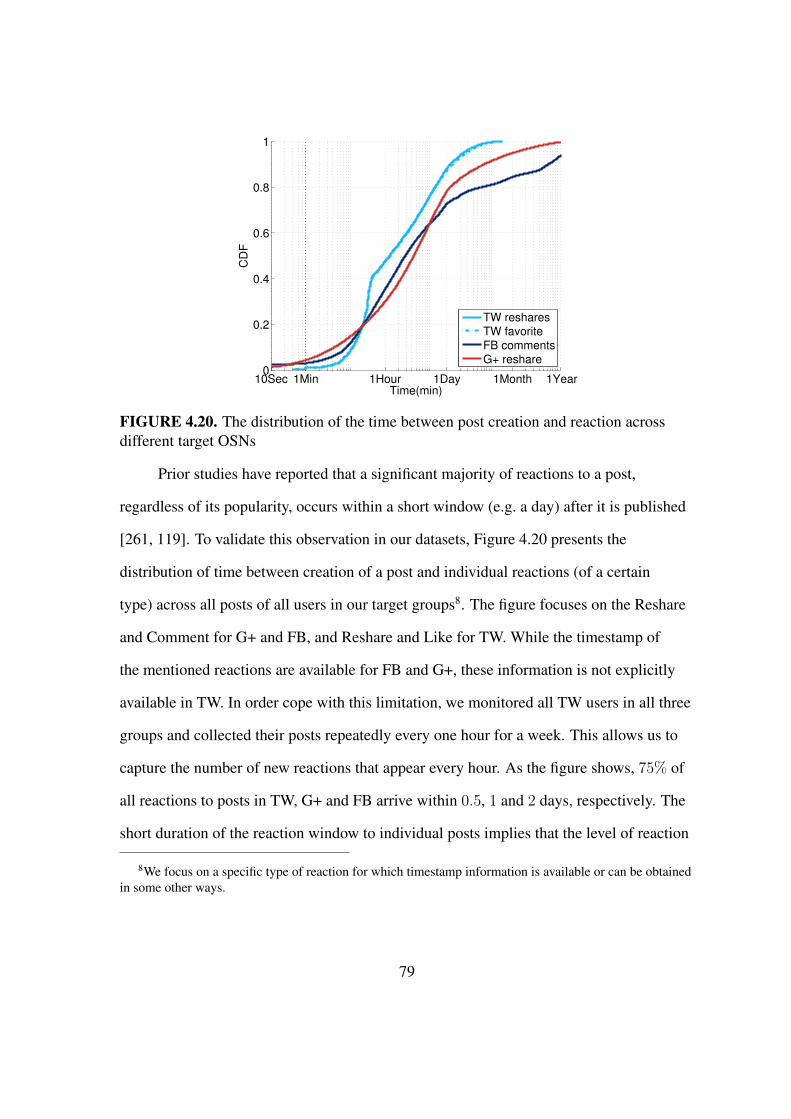
10Sec 1Min 1Hour 1Day 1Month 1Year0
0.2
0.4
0.6
0.8
1
Time(min)
CD
F
TW resharesTW favorite
FB commentsG+ reshare
FIGURE 4.20. The distribution of the time between post creation and reaction acrossdifferent target OSNs
Prior studies have reported that a significant majority of reactions to a post,
regardless of its popularity, occurs within a short window (e.g. a day) after it is published
[261, 119]. To validate this observation in our datasets, Figure 4.20 presents the
distribution of time between creation of a post and individual reactions (of a certain
type) across all posts of all users in our target groups8. The figure focuses on the Reshare
and Comment for G+ and FB, and Reshare and Like for TW. While the timestamp of
the mentioned reactions are available for FB and G+, these information is not explicitly
available in TW. In order cope with this limitation, we monitored all TW users in all three
groups and collected their posts repeatedly every one hour for a week. This allows us to
capture the number of new reactions that appear every hour. As the figure shows, 75% of
all reactions to posts in TW, G+ and FB arrive within 0.5, 1 and 2 days, respectively. The
short duration of the reaction window to individual posts implies that the level of reaction
8We focus on a specific type of reaction for which timestamp information is available or can be obtainedin some other ways.
79

to a post can be properly measured by the absolute number of reactions rather than its
rate.
Post-Level Reaction
We start by examining the distribution of the number of reactions (of each type)
to individual posts across all generated posts by users in each group that are shown in
three plots of Figure 4.19. This figure reveals the following important points: First, for
any type of reaction, only posts of Popular users typically receive a significant number
of reactions. In fact, except for the number of Likes for roughly half of the post from
Cross and Random FB users, published posts by all other non-Popular users only receive
a negligible number of reactions of any types. Specifically, the distribution of reaction per
posts across all groups are very skewed with roughly 10-15% of posts attracting 80% of
all reactions. Second, we observe that posts by Popular FB users typically attracts one to
two orders of magnitude more reactions than posts by Popular G+ users for any type of
reactions. Popular TW users attract the lowest number of Likes. Surprisingly, despite the
fact that Reshare is a common reaction type in TW, posts by Popular FB users receives
more Reshares than posts by Popular TW users. Third, for posts by Popular FB users, the
median number of Likes, Comments and Reshares is 625K, 60K and 44K, respectively.
We observe a very similar trend between different types of reactions to posts by Popular
G+ users. In contrast, the typical number of received Reshares for published posts by
TW users is more than three times larger than the number of received Likes. We note that
Like and Reshare reactions require a similar effort (i.e. one or two clicks depending on
the OSN) while Comments demand more effort (i.e. writing some text) from reacting
users. Furthermore, given the large number of followers for Popular users, the observed
reaction to their post offers a reliable view of user reactions in an OSN. Therefore, these
80

10−5
100
105
1010
0
0.2
0.4
0.6
0.8
1
Likes attracted per day
CD
F
FB
TW
G+
Popular
Cross
Random
(a) Like
10−5
100
105
0
0.2
0.4
0.6
0.8
1
Comments attracted per day
CD
F
FB
G+
Popular
Cross
Random
(b) Comment
10−5
100
105
1010
0
0.2
0.4
0.6
0.8
1
Resharers attracted per day
CD
F
FB
TW
G+
Popular
Cross
Random
(c) Resharer
FIGURE 4.21. CDF of average number of daily reactions to posts of individual users
results collectively suggests that FB and G+ users are more interested to express their own
opinion through Like and Comment reactions rather than relaying a post to other users. In
contrast, TW users are three times more likely to relay a post and facilitate its propagation
throughout the TW network. Despite this difference in the culture of reaction, a post by a
Popular FB user receives 75% more Reshares than a post by Popular TW user.
Daily User-Level Reaction
Reactions can also be viewed at the daily-rate for each user which shows the
aggregate number of reactions that a user receive to all her published posts in one day. We
refer to this view as the daily user-level reaction which is clearly a byproduct of the user’s
average daily publishing rate and the average number of reactions (of each type) to each
post. Figure 4.21 shows the distribution of daily user-level reactions across users in each
group. These distributions exhibit trends that are qualitatively similar to the distribution
of post-level reaction (shown in Figure 4.19). The only exception is the distribution of
daily user-level Reshares that is shown in Figure 4.21(c). Comparing the distribution of
daily user-level and post-level Reshare for Popular FB and TW users reveal the following
interesting point. Posts by Popular FB users typically attracts more Reshares than posts
by Popular TW users. However, because of a significantly larger activity rate among
81

Popular TW users (demonstrated in Figure 4.15), the daily user-level reaction for Popular
TW users is larger than that for Popular FB users as shown in Figure 4.21(c).
Another interesting aspect of user-level reaction is the level of balance in the
number of reactions (of any type) to different posts of individual users. To elaborate
on this issue, consider two user u1 and u2 that have a different number of posts but the
same average reaction of 50 per post. u1 receives no reaction to half of her posts and 100
reactions to each one of the other half whereas u2 receive 40 reactions per post to half
of her posts and 60 reactions to each one of the other half. In this example, the number
of reactions for u2 are more balanced than u1. We use Jain’s fairness index [144] to
quantify the level of (im)balance (or fairness) in the number of reactions across posts
of a single user. The value of 1 for Jain’s index indicate perfect balance whereas smaller
values signals a more imbalanced reactions among posts of a user. Figure 4.22 depicts the
summary distribution of Jain’s index only among users (with more than 10 posts)9 in each
candidate group. This figure reveals that: (i) The level of reaction to posts is generally
imbalanced, i.e. the index is smaller than 0.5 for a majority of users; (ii) TW users,
especially in Cross and Random groups, exhibit a very imbalanced level of reactions. In
the case of G+ users, however, half of the Popular group receive a rather balance reaction
to their posts; (iii) The level of balance in reactions is particularly diverse among Popular
FB users.
Effect of Content Type on Reactions
We investigate whether certain type of post by a particular group of users might
trigger a larger number of reactions. To do so, we split all generated posts by each group
of users across different types and examine the distribution of the number of reaction
9For a user with a smaller number of post, the index could be very noisy.
82
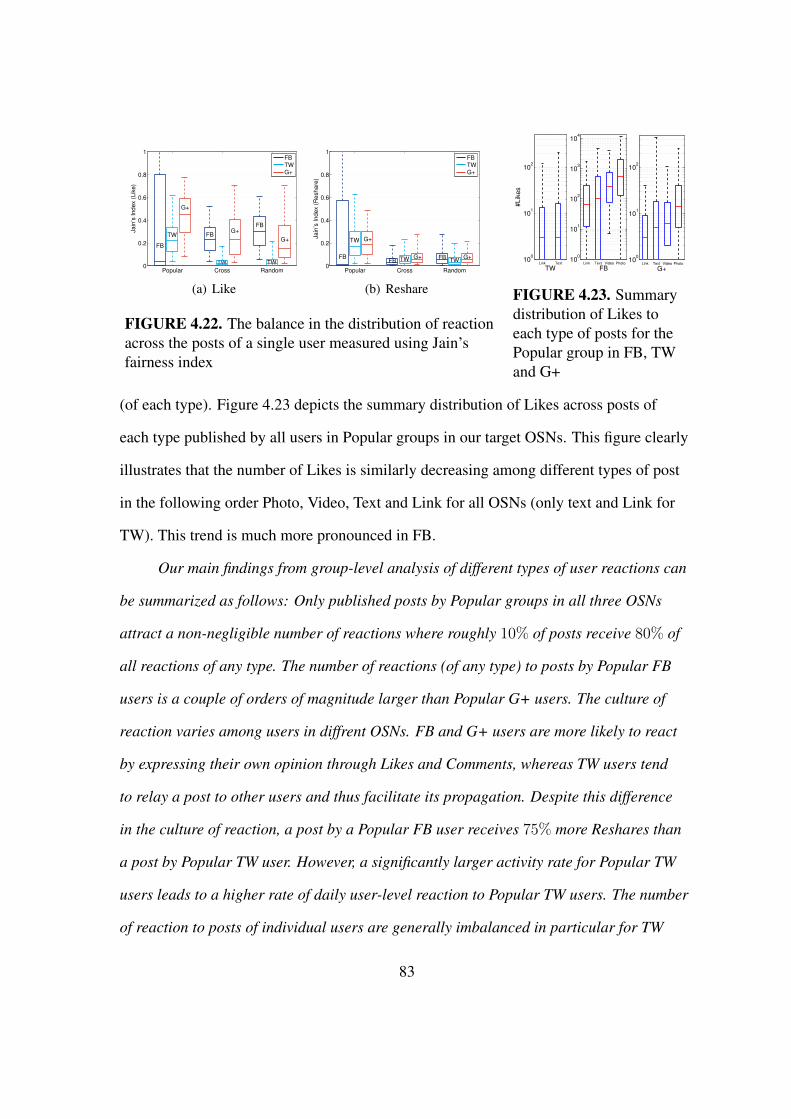
Popular Cross Random0
0.2
0.4
0.6
0.8
1
Jain
’s Index (
Lik
e)
FB
FB
FB
TW
TW TW
G+
G+
G+
FB
TW
G+
(a) Like
Popular Cross Random0
0.2
0.4
0.6
0.8
1
Jain
’s Index (
Reshare
)
FBFB
FB
TW
TW TW
G+
G+ G+
FB
TW
G+
(b) Reshare
FIGURE 4.22. The balance in the distribution of reactionacross the posts of a single user measured using Jain’sfairness index
100
101
102
TWLink Text
#L
ike
s
100
101
102
103
104
FBLink Text Video Photo
100
101
102
G+Link Text Video Photo
FIGURE 4.23. Summarydistribution of Likes toeach type of posts for thePopular group in FB, TWand G+
(of each type). Figure 4.23 depicts the summary distribution of Likes across posts of
each type published by all users in Popular groups in our target OSNs. This figure clearly
illustrates that the number of Likes is similarly decreasing among different types of post
in the following order Photo, Video, Text and Link for all OSNs (only text and Link for
TW). This trend is much more pronounced in FB.
Our main findings from group-level analysis of different types of user reactions can
be summarized as follows: Only published posts by Popular groups in all three OSNs
attract a non-negligible number of reactions where roughly 10% of posts receive 80% of
all reactions of any type. The number of reactions (of any type) to posts by Popular FB
users is a couple of orders of magnitude larger than Popular G+ users. The culture of
reaction varies among users in diffrent OSNs. FB and G+ users are more likely to react
by expressing their own opinion through Likes and Comments, whereas TW users tend
to relay a post to other users and thus facilitate its propagation. Despite this difference
in the culture of reaction, a post by a Popular FB user receives 75% more Reshares than
a post by Popular TW user. However, a significantly larger activity rate for Popular TW
users leads to a higher rate of daily user-level reaction to Popular TW users. The number
of reaction to posts of individual users are generally imbalanced in particular for TW
83
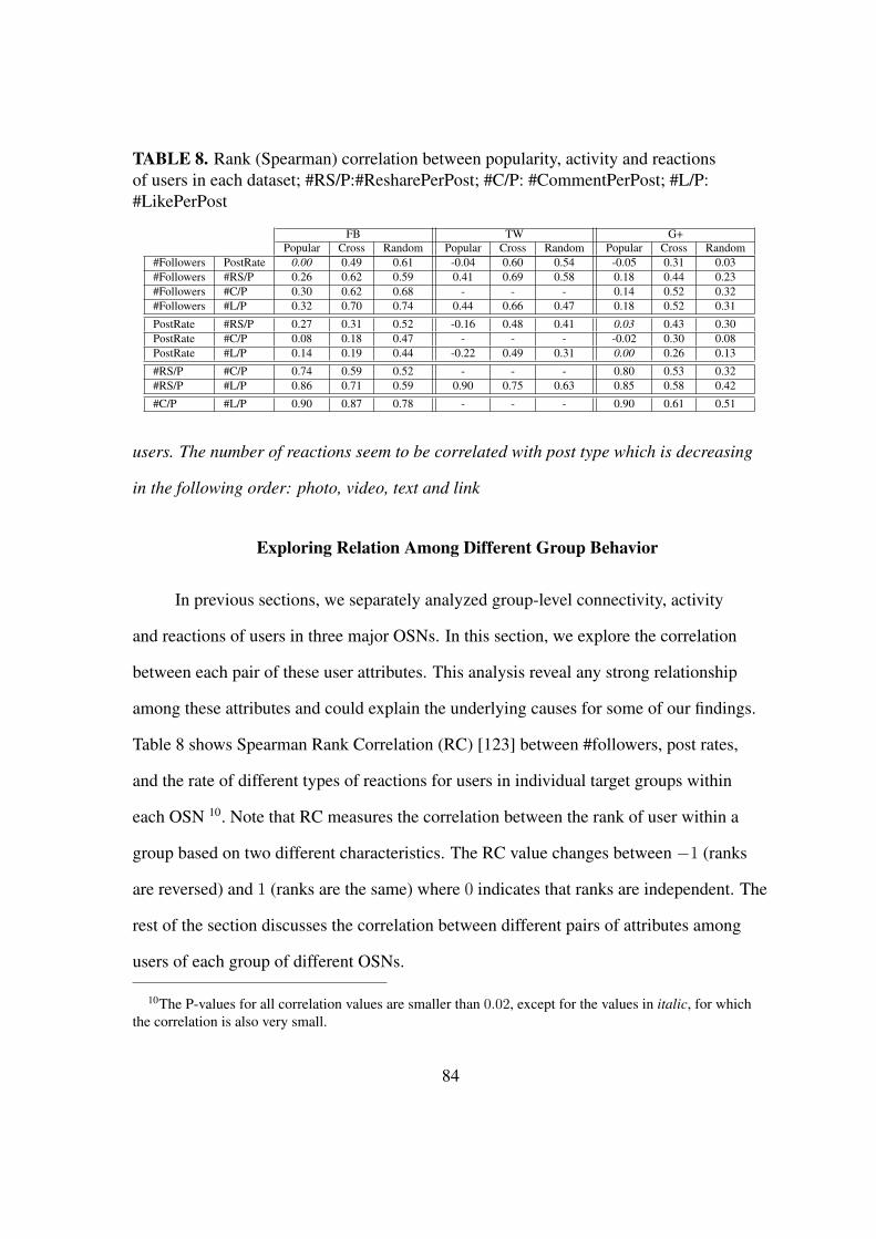
TABLE 8. Rank (Spearman) correlation between popularity, activity and reactionsof users in each dataset; #RS/P:#ResharePerPost; #C/P: #CommentPerPost; #L/P:#LikePerPost
FB TW G+Popular Cross Random Popular Cross Random Popular Cross Random
#Followers PostRate 0.00 0.49 0.61 -0.04 0.60 0.54 -0.05 0.31 0.03#Followers #RS/P 0.26 0.62 0.59 0.41 0.69 0.58 0.18 0.44 0.23#Followers #C/P 0.30 0.62 0.68 - - - 0.14 0.52 0.32#Followers #L/P 0.32 0.70 0.74 0.44 0.66 0.47 0.18 0.52 0.31
PostRate #RS/P 0.27 0.31 0.52 -0.16 0.48 0.41 0.03 0.43 0.30PostRate #C/P 0.08 0.18 0.47 - - - -0.02 0.30 0.08PostRate #L/P 0.14 0.19 0.44 -0.22 0.49 0.31 0.00 0.26 0.13
#RS/P #C/P 0.74 0.59 0.52 - - - 0.80 0.53 0.32#RS/P #L/P 0.86 0.71 0.59 0.90 0.75 0.63 0.85 0.58 0.42
#C/P #L/P 0.90 0.87 0.78 - - - 0.90 0.61 0.51
users. The number of reactions seem to be correlated with post type which is decreasing
in the following order: photo, video, text and link
Exploring Relation Among Different Group Behavior
In previous sections, we separately analyzed group-level connectivity, activity
and reactions of users in three major OSNs. In this section, we explore the correlation
between each pair of these user attributes. This analysis reveal any strong relationship
among these attributes and could explain the underlying causes for some of our findings.
Table 8 shows Spearman Rank Correlation (RC) [123] between #followers, post rates,
and the rate of different types of reactions for users in individual target groups within
each OSN 10. Note that RC measures the correlation between the rank of user within a
group based on two different characteristics. The RC value changes between −1 (ranks
are reversed) and 1 (ranks are the same) where 0 indicates that ranks are independent. The
rest of the section discusses the correlation between different pairs of attributes among
users of each group of different OSNs.
10The P-values for all correlation values are smaller than 0.02, except for the values in italic, for whichthe correlation is also very small.
84

– Connectivity vs. Activity: We observe that these two user characteristics are not
correlated for Popular groups in all OSNs (RC ≤ |0.05|). However, they exhibit a
moderate correlation among users in Cross and Random groups especially for TW
and FB (0.49 ≤ RC ≤ 0.61).
– Connectivity vs. Reactions: These two characteristics exhibit a high correlation
in FB and TW Cross and FB Random groups (0.59 ≤ RC ≤ 0.75) and moderate
correlation in TW Random and Popular as well as G+ Cross groups. This suggests
that only in these groups having more followers leads to a larger rate of reactions of
any types. For other groups, the correlation between connectivity and reaction rate
is generally positive but low (RC ≤ 0.32).
– Activity vs. Reactions: Interestingly, only FB Random and TW Cross groups show
a moderate correlation between these two characteristics (0.44 ≤ RC ≤ 0.52).
In contrast, there is no correlation between activity and any type of reaction for
Popular G+ group and even low inverse correlation for Popular TW group. All
other groups show low positive correlation.
– Different Types of Reactions: The RC between different types of reactions
indicate a significant positive correlation between all pairs in all Popular groups
(0.74 ≤ RC ≤ 0.90)). In fact, the correlation between all pairs of reactions is
at least moderate or high in all Cross group and only slightly lower in all Random
groups.
In summary, increasing the rate of activity has a moderate effect on the number of
connection (number of followers) and received reaction only in a few groups. In general,
higher level activity by a user does not lead to more reactions from others. Different types
85

of reactions are generally correlated and this correlation is more pronounced in Popular
and then Cross groups.
Temporal Analysis
So far we have examined the average user activity and received reaction during
the time that a user has participated in an OSN. These average metrics provide an
overall measure of user behavior but do not reveal any information on the short term
evolution of users activities and reactions. In this section, we examine the temporal
evolution of group-level user activities and reactions in different OSNs to compare these
characteristics of different groups over time and identify any event that affected user
behavior. We focus on daily activity or reaction over a 26-months measurement window
between January 1st 2011 and March 1st 2013. We recall that TW API only provides
the last 3 200 tweets published by users. We refer to a user who has published more than
3 200 tweets during our 26-months measurement window as a saturated user. Saturated
users make up 65%, 17% and 2% of users in Popular, Cross and Random TW groups,
respectively. The collected tweets for 90% of saturated users in Popular (and Cross)
groups represent a recent window of user activity whose length is uniformly distributed
over our measurement window.
To demonstrate this effect Figure 4.24 compares the observable with the complete
history of activity for OSNs. In these analysis we assume that users have uniform daily
activity rates over their entire age. For each date, observable history includes the non-
saturate users, whereas the complete includes the users that exist in the system (i.e. the
accounts that are created before that date). Figure 4.24(a) shows observable history
as the sum of daily post rate of users that our dataset captures in comparison to the
complete history in Figure 4.24(b) for the three systems. Figure 4.24(b) shows that the
86

J F M A M J J A S O N D J F M A M J J A S O N D J F M
101
103
105
Popular
J F M A M J J A S O N D J F M A M J J A S O N D J F M
102
104
Pos
t Rat
e of
Cap
ture
d U
sers
Cross
J F M A M J J A S O N D J F M A M J J A S O N D J F M
100
102
104
Random
Days
FB TW G+
(a) Sum of post-rates for captured users
J F M A M J J A S O N D J F M A M J J A S O N D J F M
101
103
105
Popular
J F M A M J J A S O N D J F M A M J J A S O N D J F M
102
104
Pos
t Rat
e of
Use
rs in
the
Sys
tem
s
Cross
J F M A M J J A S O N D J F M A M J J A S O N D J F M
100
102
104
Random
Days
FB TW G+
(b) Sum of post-rates for users in the three OSNs
FIGURE 4.24. The sum of the average post rate of users in the three systems incomparison to the sum of the post rate of users that we can collect their post in eachday. (The picture shows the effect of 3 200 accessible tweets.)
total daily post rate of users in TW is higher than the other systems. Therefore, when
drawing conclusions from the captured history (Figure 4.24(a)), which only shows the
daily observable post rate, extra care is needed to conclude meaningful findings.
In summary, the incomplete history of activity for saturated users indicates that the
activity (and their associated reactions) for Popular and Cross TW users are generally
underestimated in our analysis and the error is larger for earlier months. In particular, we
have the complete datasets for approximately 30 days, and from that date backwards our
dataset progressively loses TW posts due the saturated users. We carefully consider this
limitation of TW datasets in our analysis.
Evolution of Daily Activity
We start by exploring the temporal evolution of the aggregate number of daily
published posts by all users in individual groups that are shown in Figure 4.25 with
a log-scale y-axis. This figure unveils a few interesting points: First, the saw-tooth
pattern in all plots is due to the roughly 30% lower level of activity during weekends
compared to weekdays for all groups. Second, the activity rate for all groups exhibits a
generally growing trend over time but the slope of increase is much higher among Popular
87

J F M A M J J A S O N D J F M A M J J A S O N D J F M10
3
104
105
Popular
J F M A M J J A S O N D J F M A M J J A S O N D J F M10
2
103
104
Num
ber
of P
osts Cross
J F M A M J J A S O N D J F M A M J J A S O N D J F M10
1
102
103
Random
Months
FB TW G+
FIGURE 4.25. Aggregate number of posts per day (Jan. 1st 2011 - March 1st 2013)
and Cross groups. The activity rate for any TW group is consistently higher than the
corresponding FB group despite the fact that the presented rate for TW is merely a lower
bound (because of the saturated users). In fact, the gap in the activity of Popular TW and
FB groups in the last few months of our measurement appears to be widening. Third,
we observe a significant jump in the activity of all G+ groups shortly after Jun. 21, 2011
when the system was released. After this initial surge, all G+ groups exhibit a slower
growth in their activity rate compared to other groups and even appear to become flat
during some periods of time. For the activity rate of both Cross and Random groups, we
can observe a significant gap between G+ and other two OSNs that has persisted during
the entire life-time of the G+ system. This indicates that Cross users clearly prefer to
publish their posts in TW and FB rather than G+. The activity rate of the Popular G+
group has initially increased in multiple steps till it reaches close to the rate of Popular
FB and TW groups (around Feb-Jun of 2012) and has become seemingly flat during the
last nine months. This has led to an increasing gap between the activity of Popular G+
88

users and other Popular groups. With the current growth patterns, it seems unlikely that
G+ groups can close the gaps in activity with the corresponding group in FB or TW. Our
closer inspection of activity in all groups showed that both the increase in the number of
active users and the growth in the average activity of participating users has contributed
to the growing trend in their activity over time. Fourth, the time of some of the noticeable
changes in the activity rate of different groups appear to be aligned with and thus must be
caused by the following events:
– (i) Introduction of “Timeline” feature by FB (Jan. 2012): The short-term increase
in the activity of all FB groups around Jan-Feb. 2012 appears to be caused by to the
newly-introduced Timeline feature that allows users to publish their historical posts.
– (ii) Introduction of interface with 3rd-Party website by FB (Jun. 2012): The step-
like increase in the activity of Popular FB users is apparently triggered by a new
feature that allows users to share a post through a 3rd party website and collects
associated reactions on users’ FB accounts.
– (iii) Introduction of new G+ features: The step-like increases in the activity rate of
Popular and Cross G+ group are aligned with release of certain G+ features during
the first few months after its release [118].
– (iv) Holiday season: The small drop in the activity of users in all groups during the
last two weeks of Dec. is due to the holiday season.
It is intriguing that the introduction of new features in FB leads to a significant and
long-term increase in user activity whereas new features in G+ appear to create a short-
term excitement among users that quickly fades away.
89

J F M A M J J A S O N D J F M A M J J A S O N D J F M10
2
104
106
108
Popular
J F M A M J J A S O N D J F M A M J J A S O N D J F M10
2
104
106
107
Nu
mb
er
of
Lik
es Cross
J F M A M J J A S O N D J F M A M J J A S O N D J F M10
0
102
103
105
Random
Months
FB TW G+
(a) Likes
J F M A M J J A S O N D J F M A M J J A S O N D J F M10
2
104
106
Popular
J F M A M J J A S O N D J F M A M J J A S O N D J F M10
2
104
106
Nu
mb
er
of
Co
mm
en
ts
Cross
J F M A M J J A S O N D J F M A M J J A S O N D J F M10
0
102
103
105
Random
Months
FB TW G+
(b) Comments
J F M A M J J A S O N D J F M A M J J A S O N D J F M10
2
104
106
108
Popular
J F M A M J J A S O N D J F M A M J J A S O N D J F M10
2
104
106
Nu
mb
er
of
Re
sha
rers
Cross
J F M A M J J A S O N D J F M A M J J A S O N D J F M10
0
102
103
105
Random
Months
FB TW G+
(c) Resharers
FIGURE 4.26. Aggregate number of reactions per day (Jan. 1st 2011 - March 1st 2013)
Evolution of Daily Reaction
We now turn our attention to the temporal evolution of aggregate daily reactions of
each type to posts by all users in each group that is shown in Figure 4.26. We can observe
that all types of reactions to most groups (except for some G+ groups) exhibit a steady
growth with time. Apart from the initial major jump in reactions for all G+ groups, their
growth is slower than the corresponding groups in other OSNs. The main findings for
each type of reactions can be summarized as follows:
Like: Like is known to be a very popular type of reaction among FB users. Figure 4.26(a)
confirms this observation and shows that the daily rate of Likes by users in all FB groups
is a couple of orders of magnitude larger than other OSNs. The sudden increase in the rate
90

of Likes for posts in all FB groups in Jun. 2012 is aligned with the addition of 3rd party
feature by FB. Interestingly, the introduction of timeline feature by FB does not seem to
have a measurable effect on its rate of Likes despite its impact on the activity rate.
Reshares: Among all three OSNs, resharing is the most common type of reaction in
TW (retweeting). This observation coupled with the higher activity rate for all TW
groups (reported in Figure 4.25) suggest that TW groups should attract the highest rate
of Reshares. However, the daily rate of Reshare for all groups in Figure 4.26(c) depicts
a different picture. Between Jan.-Sep. 2011, the rate of attracted Reshare by Popular and
Cross TW groups is significantly higher than the corresponding groups in FB and G+11.
However, the introduction of the timeline and 3rd-party features by FB has dramatically
boosted the rate of Reshares for published posts by all FB groups since Sep. 2011. These
step-like increases are particularly visible in the number of Reshares for posts of Popular
groups. Interestingly, as a result of these two features, the rate of Reshare reactions for
all FB groups has clearly surpassed (or reached the same level as) the corresponding TW
groups despite the strong culture of Resharing (i.e., Retweeting) among TW users. We
note that while the activity and reaction rates for TW groups in the last few weeks of our
measurement window are very accurate, they are still lower than (or equal to) the rate of
corresponding FB groups. Therefore, any potential error in the activity or reaction rate of
TW groups does not affect the above conclusions.
Comments: The number of daily Comments for FB groups is much larger than G+
groups. The boosting effect of new FB features is not as visible in the daily Comments
of FB groups except for the 3rd-party feature among Popular FB users. While the number
of Comments for all FB groups has increased during our measurement period, the slope
of this increase is significantly lower than other reactions types for FB groups. The daily
11Since the TW rates could be greatly underestimated during this period, the actual gap in receivedReshares between TW and other OSNs must be even larger than what Figure 4.26(c) suggests.
91

rate of comments for G+ groups remains significantly lower than FB groups and does not
exhibit much growth for Cross and Random groups. The rate of Comments for Popular
G+ groups only show sudden increases that are clearly triggered by added features and
promotional events during the first six months after G+ was launched.
Note that any increase in the daily rate of reaction for each group is a byproduct
of the increase in the daily number of posts by its users and the growth in the average
number of reactions to their posts. Our careful examination of these two factors indicated
that the daily activity of users in each group is the primarily contributing factor that
determines the rate of received reactions (of any type) by the users. The perfect temporal
alignment between the sudden increase in the activity in FB and G+ groups with the
sudden growth in the rate of some reaction types, is another evidence that user activity
is the main determining factor for the rate of reaction.
The main findings of our temporal analysis can be summarized as follows: The
activity in all groups exhibits a persistent growth with a higher pace for Popular and
Cross groups during the past two years. This growth in the activity is driven by the
increasing number of users and the higher rate of activity among them. The activity of
all TW groups is consistently higher than the corresponding FB group and a couple
of order of magnitude larger than the corresponding G+ groups. The introduction of
new features by different OSNs (in particular FB) has led to a significant and long-term
increase in the activity of their users. The rate of Likes is much higher for FB groups and
seems to have been affected only by a the introduction of 3rd-party feature. As a result of
two newly added features by FB, the rate of observed Reshare reaction by FB users has
dramatically increased and clearly surpassed the observed rate by TW users despite the
fact that resharing is a native feature in TW. Cross users publish posts on TW at a higher
92

rate than FB, but receive a larger rate of Likes, Comments and even Reshares from FB
users.
Summary
This chapter presents a measurement-based characterization of group-level user
behavior in three major OSNs, Facebook, Twitter and Google+. We consider Popular,
Cross and Random groups of user in our analysis as they reveal a complemenary view
of user population. Our group-level approach to characterize user-behavior enables us to
compare the behavior of uses in similar groups across different OSNs or the behavior
of users in different groups of a particular OSN. We consider several aspects of user
connectivity, user activity and user reactions as three key dimensions of user behavior in
our analysis. We also conduct termporal analysis to examine short-term changes in group-
level user behavior and their potential causes. Our analysis provide a set of interesting and
insightful findings such as the following examples: (i) Only published posts by Popular
groups in all three OSNs attract a non-negligible number of reactions with a very skewed
distribution among Popular users. (ii) The number of reactions (of any type) to posts by
Popular FB users is a couple of orders of magnitude larger than Popular G+ users. (iii)
The more likely reaction by FB and G+ users is to express their own opinion whereas
TW users tend to relay a received post to other users and thus facilitate its propagation.
Despite the culture of reshare among TW users, a post by a Popular FB user receives
more Reshares than a post by Popular TW user. (iv) Added features in an OSN can
significantly boost the rate of action and reaction among its users.
We plan to extend this work in the following directions: First, we plan to examine
post content to gain a deeper insight on the published content and associated context by
individual users in each group. Second, we are conducting a more detailed study on Cross
93

group to better determine their publishing strategy in different OSNs and identify whether
they use multiple OSNs for a similar or complementary purposes.
94
CHAPTER V
“WHO’S WHO” IN TWITTER: A FIRST LOOK AT THE TWITTER ELITE
NETWORK
Accounts with the largest numbers of followers in Online Social Networks (OSNs)
such as Twitter can be viewed as “social elites”. The power-law distribution of degree
in social graphs posits that these elites are followed by many users [18, 200]. All these
elites along with their pairwise relations form a structure that we refer to as the elite
network. Despite their importance, the characterization of elite networks has received
little attention among researchers [230, 111]. As a result of the high visibility of elites
within the OSN, the elite network can be viewed as the core of the OSN social graph, thus
its characteristics offer valuable insights about the backbone of the network.
This chapter presents a detailed analysis of the micro- and macro-level structures
of the Twitter elite network. We start by explaining our methodology used to capture
a complete snapshot of the Twitter elite network that contains the 10K most followed
accounts on Twitter. We show through component analysis that a significant majority
of users in the elite networks with sizes equal to or smaller than 10K nodes form a large
strongly connected component (LSCC) and users that are not inside this component are
followed by the users in the LSCC. We identify communities of tightly interconnected
elites and show that these communities exhibit similar social and/or geographical
attributes. We further use these communities to characterize the topological structure
of elite network at the micro-level. Finally, we identify the most influential elites by
characterizing pairwise influence between them using three different measures.
95

Introduction
Recent research on OSNs is inundated with studies on their social graphs as a
whole. However, due to the large number of nodes and edges in the social graph of any
major OSN, coupled with the commonly-reported skewed distribution of user properties
(e.g. degree – number of friends and followers – and user activity), most characteristics
are dominated by users that often play insignificant social roles. This motivates our study
to shift the focus from the entirety of an OSN to a very small number of outliers that
matter the most. A small percentage of nodes with the highest degree (accounts with
the largest number of followers) in any OSN social graph can be viewed as “social elites”
since they directly influence the millions of users they are connected to or followed by.
In fact, the induced sub-graph [86] of these high degree nodes and their inter-connection
that we call elite network, can be viewed as the “core” or “backbone” of the OSN social
graph. Capturing and characterizing the connectivity structure of the elite network reveals
the key attributes of this core component. Characterizing this core component also offers
valuable insights about the impact/influence of elites on each other, which is interesting
on its own. In fact, while social scientists have extensively examined the characteristics
of elite power networks and elite influence in offline social networks [265, 89, 192, 216],
this topic has received limited attention in the context of OSNs from computer scientists.
Few prior studies focused on the elite network in major OSNs [26], and those that explore
connectivity among high degree nodes (e.g. [191]) only explored their basic connectivity
features (e.g. reciprocity, density) or focused on rich-club properties [206] by measuring
the tendency of high degree nodes to interconnect to each other. In the absence of insights
about the elite network in various OSNs, existing graph generation models for OSNs (e.g.
[18, 166, 55]) do not incorporate any requirement for the connectivity features among
96

high degree nodes (i.e. elites). Therefore, the backbone of their resulting graphs do not
properly represent the structure of a typical OSN [25].
Additionally, since many regular users directly follow at least a few elites, elite
users can serve as landmarks for clustering regular users in the OSN as well. Therefore,
the characterization of the elite network potentially leads to impactful findings, not only
about about elites, but also about the OSN as whole.
In this chapter, we tackle the following three fundamental questions about the
elite network in a major OSN, namely Twitter: (i) What are the macro- and micro-level
structural characteristics of the Twitter elite network? (ii) What insights can be gained by
studying the elite networks about the entire graph? (iii) How can we assess the influence
among Twitter elites?
In Section 5.2, we describe our technique for identifying the top 10K Twitter
accounts with the largest number of followers and the pairwise directed friend-follower
connections among them. The resulting social sub-graph among the top 10K Twitter
accounts enables us to examine the Twitter elite network at different sizes (smaller than
10K). Furthermore, we obtained the social category and country information for these
accounts along with their profile information and all the available tweets for all 10K
elite accounts. The “view” n-ELITE is defined as the Twitter elite network which is the
graph of friend-follower relationships between the top-n most followed accounts. We use
these views to study the elite network and examine how various characteristics of the elite
network evolves as less popular elites are included in the elite network.
In Section 5.3, we explore the macro structure of the Twitter elite network. In
particular, we show that the elite network, regardless of its size, is a single weakly
connected competent, but has multiple strongly connected components where 90%+ of
the nodes are located in the largest strongly connected component (LSCC). Furthermore,
97

the elite network exhibits an “onion-like” layered structure where users with more
followers have the highest PageRank centrality values as well (calculated on the elite
network). Hence, the most followed elites are at the core and less popular elites form
layers around the core.
We then focus on the structure of the elite network in Section 5.4 at the community
level. Toward this end, we first motivate and define the notion of resilient community
[57, 229] and then identify such communities (and their associated nodes) among elites
as well as a group of unstable nodes that includes accounts that do not belong to a single
community in each of the views of the elite network. Leveraging the social and country
attributes of individual elites, we demonstrate that the identified communities exhibit a
strong social cohesion (i.e. clear social theme among accounts in resilient communities).
This in turn confirms that these communities represent meaningful units of the elite
network. We further explore how these communities evolve as one extends the size of
the elite network to include less popular accounts. We characterize relative connectivity
and coupling between communities which in turn reveals an inter-community structure (or
inter-community interest) in the elite network. Furthermore, we demonstrate that unstable
nodes act as “hubs” as they sit between two or more elite communities and also identify
community members who serve as bridges to other communities.
Finally, we investigate the influence of individual elites on the rest of the elite
network in Section 5.5. Similar to prior studies [59] we use different measures, namely
PageRank, retweet and reply to capture influence over other elites. We argue that the
number of retweets and replies are not necessarily enough to capture the influence and
that the number of elites who have been influenced is also an important factor. We
determine the aggregate influence of an individual elite on the rest of the elite network
and show the factors that affect the measured influence. We then identify the list of top-
98

N most influential users based on each measure and examine the overlap among them as
a function of N. We show that the top-10 most influential accounts based on PageRank,
Retweet, and Reply are mostly political/corporate elites, news media and magazines, and
gossip/entertainment celebrities, respectively. Section 5.6 summarizes and concludes this
chapter.
Capturing the Elite Network
Our goal is to capture the Twitter elite network - that is a subgraph of Twitter that
includes the top-N most-followed accounts (i.e. node with the highest (out)degree) and
the relationships among them (i.e. edges)1. Furthermore, we need to annotate each node
with its social and geographical (location) attributes in order to explore the impact of
these attributes in relationships among elites. There are a few issues that we need to
address before we achieve this goal as follows. First, we need to specify the minimum
number of followers that qualifies a user as an elite. Second, we need to efficiently
identify all of the qualified Twitter accounts, their attributes, and the connections (e.g.
friend-follower relationship) among them. In particular, since these users have millions of
followers, it is prohibitively expensive to find all their pairwise connections by collecting
and examining all their followers.
To cope with these challenges, our data collection strategy for capturing Twitter
elite network consists of the following four steps:
1. Capturing a list of most-followed Twitter accounts through public resources and
random walks used as seeds.
2. Inferring their pairwise connections.
1We use the terms nodes with highest degree and most followed accounts interchangeably.
99

3. Identifying missing accounts, validating the information, and collecting pairwise
connections.
4. Collecting all profile information and available tweets of discovered accounts.
The details of individual steps are as follows:
Step 1: To bootstrap the data collection process, we crawl lists of the most
followed accounts from online resources. In particular, marketing websites such as
socialbakers.com offer professionally maintained lists of most followed accounts in
variety of OSNs in different social categories (e.g. celebrities, actors, sport, community,
...). Each list on socialbakers.com provides up to 1000 top accounts in the selected
category along with the number of followers and username for each account. We collect
the list associated with all offered categories and subcategories and create a unified list
that includes all the uniquely-discovered user accounts with their number of followers
(and associated rank), their category and location. This resulting unified list consists of
59 832 unique users whose number of followers varies from 263 to 81M, and they are
associated with 123 categories and 191 unique countries.
We also conduct approximately 2K random walks on the list of friends from
randomly selected Twitter accounts to identify high-degree nodes. The theory of random
walk [173] indicates the likelihood of a visit by a walker to a node is proportional to the
degree of that node in the graph. Therefore, random walks offer an efficient technique to
identify highest degree nodes [248, 215].
Equipped with these two techniques to identify potential highest degree nodes,
we then create a master list that includes more than 60K accounts. We mainly focus
on the top 10K accounts with the most followers from this master list. In this list, 89%
are exclusively reported on socialbakers.com, 3.2% are exclusively identified through
random walks, and 7.8% are found through both techniques. It is worth noting that the
100

overall popularity rank of the accounts exclusively found by random walk is at least 133
out of 10K.
Step 2: To collect all the connections among the identified accounts in the previous
step, our key observation is that the number of friends for elites are almost always
several orders of magnitude smaller than the number of followers. Therefore, instead
of followers, we collect the complete list of friends for each selected account from Twitter
(using its API). This implies that the connection between account ufri and its follower
account ufol (denoted as ufri → ufol) is discovered when we collect the friend list of
account ufol, i.e. each edge is discovered from the follower side. This simple observation
ensures that all pairwise connections among the selected accounts are identified efficiently
(without collecting all followers of all accounts). The total number of crawled friend-
follower relationships for all elite accounts is 504.8M which consists of 95M unique
friends for the top 10K most-followed elites.
Step 3: At this point, we have a snapshot of the most-followed Twitter accounts
and their pairwise directed connections. It is indeed possible that the identified top 10K
accounts from online sources supplemented with the the list collected from random walks
do not accurately capture the top 10K accounts on Twitter, i.e. some elite accounts might
be missing. We take a few steps to verify whether the collected information is correct
and complete. Our final step is similar to the approach proposed by Avrachenkov et al.
[27]. The observation is that any such missing elite account should be followed by many
elites already identified as top 10K accounts. Note that we already obtained the entire list
of friends for top 10K accounts. We calculate the number of elite-followers for all these
collected friends that are not among the elites, and sort the resulting list by the number of
elite-followers. We start by scanning this list from the top and collect account information
including the number of followers for users in this list. If the number of followers for
101

any of these accounts is larger than the number of followers for the account at rank 10K,
we add it to the master list (at the proper rank) and update the ranks for all elites. We
continue this process until 100 consecutive accounts from this sorted list do not make
it to the master list. We finally identify the edges between these accounts and other
top 10K accounts by collecting their friend list. Using this technique, we detected 264
accounts that are between the rank of 500 and 10K among the top 10K accounts. The
small percentage of missing accounts along with their relatively low ranking indicate
that our master list is accurate. All in all, among the top 10K most followed accounts,
8 704 were exclusively reported in socialbakers.com, 301 were found exclusively using
random walks, and 731 are from both the mentioned resources. Finally, checking the
most followed friends of elites placed 264 new elites on the list of top 10K most followed
elites.
Step 4: We collect all the available tweets for the top 10K Twitter accounts. The
available tweets2 for each account are used to investigate the influence between elites and
gain some insight on how they use Twitter.
Who is Elite?
It is certainly compelling to consider Twitter users with the highest number of
followers as Twitter elites. One remaining question is how many most-followed accounts
should be considered for forming the elite network? We argue that the 10K-ELITE offers
a significantly large view of the elite network in Twitter for several reasons as follows:
First, the skewed distribution of the number of followers implies that the number of
followers rapidly drops with rank. For example, the top 10 most followed accounts
have between 51.9M to 81.7M followers while the last 10 accounts in the top 10K have
2Twitter only provides the last 3 200 generated tweets by each user.
102
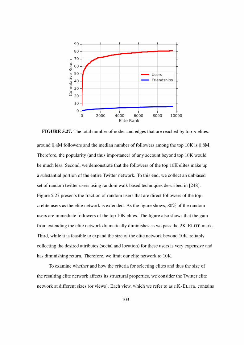
0 2000 4000 6000 8000 10000Elite Rank
0
10
20
30
40
50
60
70
80
90
Cum
ula
tive R
each
Users
Friendships
FIGURE 5.27. The total number of nodes and edges that are reached by top-n elites.
around 0.4M followers and the median number of followers among the top 10K is 0.8M.
Therefore, the popularity (and thus importance) of any account beyond top 10K would
be much less. Second, we demonstrate that the followers of the top 10K elites make up
a substantial portion of the entire Twitter network. To this end, we collect an unbiased
set of random twitter users using random walk based techniques described in [248].
Figure 5.27 presents the fraction of random users that are direct followers of the top-
n elite users as the elite network is extended. As the figure shows, 80% of the random
users are immediate followers of the top 10K elites. The figure also shows that the gain
from extending the elite network dramatically diminishes as we pass the 2K-ELITE mark.
Third, while it is feasible to expand the size of the elite network beyond 10K, reliably
collecting the desired attributes (social and location) for these users is very expensive and
has diminishing return. Therefore, we limit our elite network to 10K.
To examine whether and how the criteria for selecting elites and thus the size of
the resulting elite network affects its structural properties, we consider the Twitter elite
network at different sizes (or views). Each view, which we refer to as nK-ELITE, contains
103

0 1 2 3 4 5 6 7 8 9Rank (thousands)
0.0000
0.0002
0.0004
0.0006
0.0008
0.0010 PageRank
(a) Nodes PageRanks grouped byrank
0 1 2 3 4 5 6 7 8 9Rank (thousands)
0.0005
0.0000
0.0005
0.0010
0.0015 PageRank Difference
(b) Difference in PageRank foredges
FIGURE 5.28. PageRank of elites in 10K-ELITE grouped by their rank; Difference inPageRank of follower-friend at both ends of each edge in 10K-ELITE, grouped by therank of the friends
the top n-thousand most-followed accounts and friend-follower relationships between
them.
Our final argument with respect to the size of the elite network lies in its structure
as a graph as it extends to cover less popular elites. The question that helps characterize
this extension is “whether the centrality of individual elites in the elite network is a
function of their overall popularity (i.e. total number of followers)?” Given the directed
nature of the elite network, we compute the PageRank [207] of each node as a measure
of its centrality3. Figure 5.28(a) shows the summary distribution of nodes’ PageRanks
computed over the 10K-ELITE presented as boxplots. In this plot, nodes are grouped
according to their rank based on the number of followers in buckets each one with 1K
nodes. In essence, each group represents the new set of nodes that are added to each
view to create the next extended view. This figure reveals a pattern where the PageRank
centrality of elites in the elite network generally decreases with their overall popularity.
3We computed PageRank on a network with inverted edges, to ensure that PageRank values correspondwith importance and reasonable definition of centrality.
104

We also included a similar plot for the difference in the PageRank of users at the ends of
each edge in 10K-ELITE in Figure 5.28(b). Similar to the previous analysis, all edges are
grouped into 10 buckets according to the rank of the friend and the summary distribution
presents PageRankfri − PageRankfol. We observe that as we go to buckets that contain less
popular elites, the the difference between the centrality of friend and follower decreases.
These two figures suggest that elites form an “onion-shape” structure where the highest
ranked elites are in the center, and other groups with lower ranks form layers around the
core. Most friend-follower relationships (directed edges) have their friend side in the
inner layers and the follower side in the outer layers. This result supports our choice of
the size of the elite network, since the plot demonstrates the PageRank of elites at lower
rank buckets are effectively similar. Therefore, including more elites only adds more
layers around this onion-like topology structure.
In summary, our data collection pipeline is capable of identifying the top 10K most
followed Twitter accounts and all their friend-follower relationships, i.e. 10K-ELITE.
More than 80% of the users in Twitter follow at least one account in 10K-ELITE, and
including less popular accounts seems to have a minimal effect on the reach of 10K-
ELITE. Additionally, this network exhibits an “onion-shape” structure, with more popular
elites in the center of the network and less popular elites forming outer layers. Most elites
in the outer layers are following elites in the inner layers, but are being followed by elites
in close by layers.
Macro-Level Structure
Before we conduct any analysis on the Twitter elite network, we present a number
of basic characteristics for each view of the elite network in Table 9, including the number
of nodes and directed edges (|E|), reciprocity (Rcp), transitivity or clustering coefficient
105

TABLE 9. Basic characteristics of the elite networks and their weakly and stronglyconnected components
CC SCC
View |E| Rcp Tran Diam #CC %|V | %|E| #SCC %|V | %|E|
1K-ELITE 49K 0.35 0.3 7 1 100.0 100.0 64 93.5 94.62K-ELITE 126K 0.34 0.24 7 2 100.0 100.0 110 94.2 95.63K-ELITE 231K 0.32 0.2 7 3 99.9 100.0 171 94.1 95.84K-ELITE 344K 0.31 0.18 7 3 100.0 100.0 231 94.0 95.95K-ELITE 491K 0.32 0.17 7 3 100.0 100.0 279 94.2 96.16K-ELITE 648K 0.33 0.16 7 2 100.0 100.0 337 94.1 96.27K-ELITE 816K 0.34 0.16 7 2 100.0 100.0 370 94.5 96.48K-ELITE 1.0M 0.37 0.17 7 2 100.0 100.0 401 94.8 96.79K-ELITE 1.2M 0.4 0.18 8 2 100.0 100.0 439 94.9 96.910K-ELITE 1.4M 0.42 0.19 9 2 100.0 100.0 454 91.5 97.0
(Tran), and diameter (Diam). We also include the number of connected components and
strongly connected components. This table clearly shows that as the size of the elite
network is extended (from 1K to 10K), it becomes denser (average degree increases from
49 to 152), the fraction of reciprocated edges initially drops and then increases, and its
diameter slightly increases. In all views, 32-40% of the friend-follower relationships are
reciprocal, which is higher compared to the reported 22% for the entire Twitter social
graph [163]. Interestingly, we observe that all views of the elite network have a single
weakly connected component that includes an absolute majority of all nodes except for
one or two nodes. However, the number of strongly connected components (SCC) grows
roughly proportional with the size of the elite network. The rank correlation between
the number of public vs. elite followers for top-10K elite is around 0.55 while the rank
correlation between their public vs. elite friends is 0.1, i.e. the popularity of elites among
all users and elites are moderately correlated.
106

3
935
(a) 1K-ELITE
2
2
2
2
22
2
2
2
2
2
4
4708
(b) 5K-ELITE
2
2
2
22
2
2
2
2
2
2
4
4
4
2
9146
(c) 10K-ELITE
FIGURE 5.29. The connectivity of strongly connected components of the elite networks
Overall Structure of the Social Graph
In this section, we conduct (strongly) connected component analysis [97] on
different views of the elite networks in order to reveal their overall topological structure.
As we reported in Table 9, each view of the elite network has many strongly connected
components (SCC). However, the largest strongly connected component (LSCC) in
each view contains an absolute majority of all elites while all other SCCs have a single
node (and in a few cases a handful of nodes). The right section of Table 9 summarizes
the fraction of nodes and edges that are within the LSCC in each view. This table shows
that the LSCC in each view contains 91-94% of all nodes and 94-97% of all edges of the
corresponding elite network.
To gain more insight into the structure of the elite network, Figure 5.29 visualizes
the strongly connected component structure of 1K-ELITE, 5K-ELITE, and 10K-ELITE
as directed graphs where each circle represents a SCC with the number indicating the
number of nodes in that SCC. LSCC is shown with a green circle in the center. Arrows
represent friend→follower relationships between users in different SCCs. These figures
clearly illustrate that in all views the SCCs form a “star-like” structure where the LSCC
is in the center and there are a number of directed edges from every other SCC (that we
107

6K..7K
9K..10K
4K..5K
5K..6K
2K..3K
3K..4K
8K-OSCC
2K-LSCC
1K-LSCC
1K-OSCC
1K..2K3K-LSCC
4K-LSCC
5K-LSCC
6K-LSCC
10K-OSCC
10K-LSCC
9K-LSCC
8K-LSCC
7K-LSCC
8K..9K
7K..8K
9K-OSCC2K-OSCC 3K-OSCC 4K-OSCC 5K-OSCC 7K-OSCC6K-OSCC
FIGURE 5.30. The dynamics of LSCC as the network expands
call “outsider”) to nodes in LSCC. We recall the direction of edges are from a friend
to a follower (or the direction of tweet propagation.) Therefore, Figure 5.29 indicates
that nodes in the LSCC have an interest in and receive tweets from nodes in other
SCCs (through the elite network) but the opposite is not true. In fact, more than 99% of
outsiders are followed by users in the LSCC. Most outsider nodes are in a single node
SCC and few of them consist of two or more nodes. For example, the Pope has four
accounts that only follow each other but they are followed by many accounts inside the
LSCC.
As more nodes are included in the view of the elite network, other SCCs in one
view may be pulled into the LSCC in the next view since the extended view may include
more shortcuts. Figure 5.30 illustrates via Sankey diagram [5] how the LSCC and the
outsider in each view are mapped/split to the LSCC and the outsider in the next view4.
In this figure individual views of the elite network are shown along the x axis. For
each view, the two vertical boxes represent LSCC and the outsider. The vertical box at
the bottom of each column represents the LSCC and the box on the top represents the
4An interactive visualization of this diagram is available on our project pageix.cs.uoregon.edu/˜motamedi/research/elite/evol/sankey_in_out_lscc.html
108

outsider. Groups of elites ranked by their number of followers are all presented in the first
column alongside 1K-ELITE. Extending the elite network adds one of the groups to a
view to create the next view, for instance accounts with rank [1K..2K] join 1K-ELITE to
create 2K-ELITE. As the plot shows, more than 95% of these newly added elites join the
LSCC and the rest join the other SCCs. An examination of these views also reveals that
roughly 13-20% of nodes in other SCCs are pulled into the LSCC in the next view. Note
however that a group of other SCCs have no friends (i.e. no incoming edges) and thus
remain outside the LSCC regardless of the size of the elite network.
Micro-Level Structure
In this section, we characterize the connectivity structure of the elite network at the
community level.
Detecting Communities Among Elites
We start by exploring whether there are groups of tightly connected nodes (or
communities) inside the network and then use these communities as the basic elements
to explore the coarser representation of each view of the elite network.
There are two basic issues in identifying communities in the elite networks. First,
most commonly-used community detection techniques take undirected graphs as input
while the elite network is a directed graph [107]. To address this issue, we first convert
each view of the elite network into an undirected graph by turning each directed edge
into a single undirected edge, therefore connecting nodes with two undirected edges (or
an edge with the weight of 2) when reciprocal edges exist. This representation allows us
to encode tighter binds between users with reciprocal edges. Our approach is therefore
different from prior studies (e.g. [169]) where they simply consider a directed graph
109

as undirected. Second, the outcome of the most commonly used community detection
techniques (e.g. Louvain [40], BigCalmm [276], InfoMap [222]) is non-deterministic.
More specifically, multiple runs of a single algorithm on the same graph produce different
numbers of communities and/or different grouping of nodes into communities. Our
empirical stability comparison of a few well-known community detection algorithms
showed that COMBO results in communities with more stable mapping of nodes to
those communities while maximizing the community modularity, i.e. the identified
communities in various runs are more similar compared the detected communities by
other techniques. To address the stability issue, we use COMBO [240] that relies on multi-
objective optimization to find tight communities. We only consider a group of nodes as
a community if they consistently mapped to the same community across different runs.
Toward this end, we adopt the following strategy: We run the community detection
technique on each view of the elite network k times and determine the communities
that individual nodes are mapped to in each run in a vector with k values, called the
“community vector”. Then, we group all the nodes that are consistently (i.e. all k times)
mapped to the same community (i.e. have the same community vector) and refer to the
group as a Resilient Community. The process of detecting communities also results in
groups of nodes for which no other node has the same community vector. We group this
set of nodes and nodes in resilient communities with a size smaller than 10 and refer to
them as Unstables. Therefore, unstable nodes are those that have none to only a few other
nodes in their resilient community. These unstable nodes have the tendency to be grouped
with other resilient communities of nodes as a single traditional community across
different runs, and therefore can not be considered as a part of any resilient community.
Clearly increasing k is more restrictive and may lead to smaller resilient
communities since more runs can simply split a community to two (or more) smaller
110

ones. Figure 5.31 shows the effect of k on the number of resilient communities identified
in 1K-ELITE, 5K-ELITE and 10K-ELITE. As the figure shows, increasing k can split
resilient communities and increase the number of resilient communities. This number
may shrink, however, when the newly created resilient communities include less than the
minimum threshold size of resilient communities, which we set to 10. Note that in all runs
of COMBO, a community smaller than 20 nodes was never identified, i.e. our threshold
does not dissolve a community in the unstable group. It is also interesting to note that
the effect of increasing k is more considerable in 5K-ELITE. This indeed suggests that
this view has a less pronounced community-level structure since each run leads to the
identification of a very different grouping of nodes as communities [57]. Figure 5.31
also shows that in all cases the number of resilient communities stabilizes after the initial
increase. We conservatively consider k = 100 in our analysis, as having more runs does
not lead to the identification of more resilient communities in the elite networks. Since the
term “community” is the well accepted term to refer to a group of nodes that are tightly
connected, we simply use the term “community” to refer to a resilient community, and
when necessary use term “traditional community” to specifically refer to a community
identified in a single run of the community detection algorithm.
Table 10 presents the general statistics of the communities identified in each view.
As the table shows, COMBO detects different numbers of communities in each run. The
minimum and maximum number of detected traditional communities are reported in the
table. Note that detecting the same number of communities does not mean that the run
of COMBO lead to the same splitting of nodes across communities. Using the previously
described approach, we identified between 10 to 29 resilient communities with 10+ nodes
that collectively cover 92-99%+ of all the nodes in each view of the elite network. Thus,
111

0 20 40 60 80 100runs
10
15
20
25
# R
esi
lient
Com
munit
ies
1K-ELite
5K-ELite
10K-ELite
FIGURE 5.31. The number of identified resilient communities as a function of k in threeviews of the elite network.
less than 8% of the elites are categorized as the unstables and this percentage in 10K-
ELITE is only 1.6%.
We should reemphasize that the identified communities in (different views of)
the elite network could hypothetically be very different from communities on the entire
Twitter social graph that contain many regular (i.e. non-elite) users. Later in this chapter
we discuss and demonstrate that these identified communities provide a great potential for
identifying communities among regular users as well.
Resilient vs. Traditional Communities
It is not clear if the resilient communities contain groups of well-knit nodes inside
the community with a low level of interconnection to other resilient communities. To
examine whether resilient communities exhibit different connectivity/size characteristics
compared to regular communities, which in turn could affect the result of our community-
based analysis, we compare the identified communities and traditional communities. We
use conductance [41] and modularity [201] as two measure of a graph structure with
respect to the identified communities in the graph. Conductance measures how well a
112

TABLE 10. General statistics of communities identified in each view.
Min Trad. Com. Max Trad. Com. Res. Com. % Unstable
1K-ELITE 6 7 12 7.92K-ELITE 7 9 20 8.03K-ELITE 8 9 11 2.54K-ELITE 9 10 16 4.05K-ELITE 8 10 22 6.56K-ELITE 8 9 29 5.57K-ELITE 9 11 13 2.48K-ELITE 8 8 11 1.79K-ELITE 8 9 10 1.210K-ELITE 8 9 14 1.6
certain bipartition of nodes splits in the graph. Therefore, for each community – a cut
through the edges in the graph – we can compute a single conductance value. Small
conductance values mean that a small number of edges are cut to split the graph into
two halves (i.e. the community and the rest of the graph). On the other hand, modularity
measures how well a graph divides into modules. In other words, a graph with high
modularity computed for a certain grouping of nodes into modules (communities) has
dense connections between the nodes within modules, but sparse connections between
nodes in different modules. For each graph partitioning into communities a single
modularity is computed.
We separately identified communities in each view of the elite network. Figure 5.32
shows the scatter plot of conductance and size of traditional communities identified in all
100 runs of COMBO, the resilient communities, and also the unstables in the 10K-ELITE
view. We recall that smaller conductance suggests a better separation of the community
from the rest of the graph. A close comparison of the communities with the identified
traditional communities shows that for similar sizes, their conductance values are indeed
smaller or similar. There are only two rather small resilient communities that higher
113
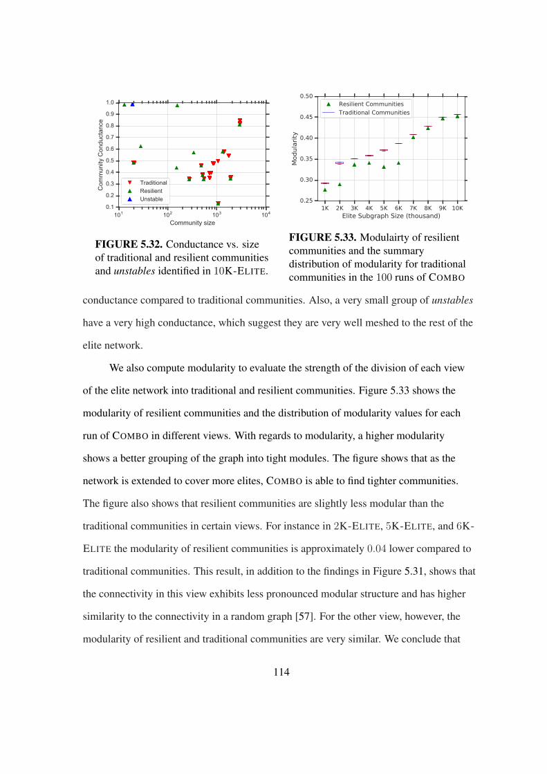
101 102 103 104
Community size
0.1
0.2
0.3
0.4
0.5
0.6
0.7
0.8
0.9
1.0C
omm
unity
Con
duct
ance
TraditionalResilientUnstable
FIGURE 5.32. Conductance vs. sizeof traditional and resilient communitiesand unstables identified in 10K-ELITE.
1K 2K 3K 4K 5K 6K 7K 8K 9K 10KElite Subgraph Size (thousand)
0.25
0.30
0.35
0.40
0.45
0.50
Modula
rity
Resilient Communities
Traditional Communities
FIGURE 5.33. Modulairty of resilientcommunities and the summarydistribution of modularity for traditionalcommunities in the 100 runs of COMBO
conductance compared to traditional communities. Also, a very small group of unstables
have a very high conductance, which suggest they are very well meshed to the rest of the
elite network.
We also compute modularity to evaluate the strength of the division of each view
of the elite network into traditional and resilient communities. Figure 5.33 shows the
modularity of resilient communities and the distribution of modularity values for each
run of COMBO in different views. With regards to modularity, a higher modularity
shows a better grouping of the graph into tight modules. The figure shows that as the
network is extended to cover more elites, COMBO is able to find tighter communities.
The figure also shows that resilient communities are slightly less modular than the
traditional communities in certain views. For instance in 2K-ELITE, 5K-ELITE, and 6K-
ELITE the modularity of resilient communities is approximately 0.04 lower compared to
traditional communities. This result, in addition to the findings in Figure 5.31, shows that
the connectivity in this view exhibits less pronounced modular structure and has higher
similarity to the connectivity in a random graph [57]. For the other view, however, the
modularity of resilient and traditional communities are very similar. We conclude that
114

resilient communities each contain a group of nodes with a large number of social ties
within the resilient community and a small number of friendships with users in other
resilient communities.
Social/Geo Footprint of Communities
In this section, we address the root cause of community formation in the elite
network. Our focal question is “do nodes in a community exhibit any social cohesion?”
Answering this question reveals whether the identified communities represent meaningful
elements of the elite network or not. It is worth reminding that approximately 90% of
elites are collected from socialbakers.com. This resource tags each account with 8
categories, 137 subcategories and 196 countries. To tackle the problem at hand, we
leverage this category and location information that we collected for elites. We present
two histograms that show the number of nodes across 10 most common categories (i.e.
social footprint) and countries (i.e. geo footprint) in each community. Figure 5.34 depicts
the social and geo footprints for the 9 largest communities in 10K-ELITE. The footprints
of these communities exhibit varying levels of social and/or geo (or language) cohesion.
Since many of these accounts belong to easily recognizable individuals/entities, we can
also examine the identity of accounts in each community and use their social context to
learn more about the “theme” associated with each community5.
Here we describe the dominant themes in the 10 largest communities in 10K-
ELITE. The number in the parenthesis following each community name is the number
of accounts in that community.
C1 - US Popstar (2799): This community is associated with celebrities, popstars and
entertainment media. The vast majority of these elites are from the US with the remainder
5The identity of accounts mapped to individual community in each view are available online at ix.cs.uoregon.edu/˜motamedi/research/elite/tables/elite10000_20160112 for readers.
115
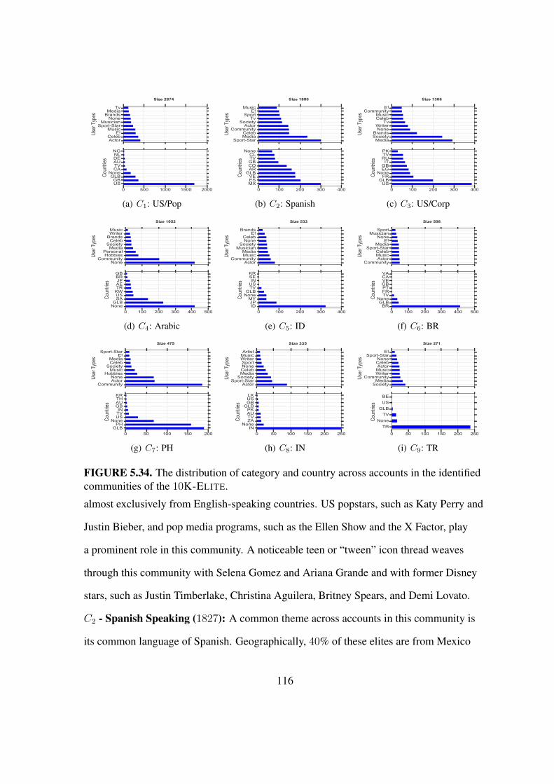
ActorCeleb
E!Music
Sport-StarMusician
NoneBrandsMedia
Tv
User
Typ
es
0 500 1000 1500 2000USGB
GLBNone
CATVAUDENLNG
Coun
tries
Size 2874
(a) C1: US/Pop
Sport-StarMediaCeleb
CommunityActor
SocietyTv
SportE!
Music
User
Typ
es
0 100 200 300 400MXESVE
GLBARCOGBTVCL
None
Coun
tries
Size 1880
(b) C2: Spanish
MediaSocietyBrands
NoneWriter
TvCelebMusic
CommunityE!
User
Typ
es
0 100 200 300 400US
GLBFR
NoneEGGB
ITRUTVPK
Coun
tries
Size 1306
(c) C3: US/Corp
NoneCommunity
HobbiesPersonal
MediaSociety
CelebBrandsWriterMusic
User
Typ
es
0 100 200 300 400 500NoneGLB
SAUSKWTRAEJPBRGB
Coun
tries
Size 1052
(d) C4: Arabic
ActorCommunity
MusicMedia
MusicianSociety
NoneCeleb
E!Brands
User
Typ
es
0 100 200 300 400IDJP
MYNoneGLB
TVUSIN
SEKR
Coun
tries
Size 533
(e) C5: ID
CommunityActorMusicCeleb
Sport-StarMedia
E!None
MusicianSport
User
Typ
es
0 100 200 300 400 500BR
GLBNone
TVFRPTGBVECAVA
Coun
tries
Size 508
(f) C6: BR
CommunityActorNone
HobbiesMusic
SocietyCelebMedia
E!Sport-Star
User
Typ
es
0 50 100 150 200GLB
PHNone
USTVIN
GBAUTHKR
Coun
tries
Size 475
(g) C7: PH
ActorSport-Star
SocietyMediaCelebNoneSportWriterMusicArtist
User
Typ
es
0 50 100 150 200 250IN
NoneZATVAUPK
GLBGBUSLK
Coun
tries
Size 335
(h) C8: IN
SocietyMedia
CommunityWriterMusicActor
CelebNone
Sport-StarE!
User
Typ
es
0 50 100 150 200 250
TRNone
TVGLB
USBE
Coun
tries
Size 271
(i) C9: TR
FIGURE 5.34. The distribution of category and country across accounts in the identifiedcommunities of the 10K-ELITE.
almost exclusively from English-speaking countries. US popstars, such as Katy Perry and
Justin Bieber, and pop media programs, such as the Ellen Show and the X Factor, play
a prominent role in this community. A noticeable teen or “tween” icon thread weaves
through this community with Selena Gomez and Ariana Grande and with former Disney
stars, such as Justin Timberlake, Christina Aguilera, Britney Spears, and Demi Lovato.
C2 - Spanish Speaking (1827): A common theme across accounts in this community is
its common language of Spanish. Geographically, 40% of these elites are from Mexico
116

and 30% are from Spain. Yet, the geographic distribution draws from a wide swath of
both Spanish-speaking elites with a small, but important group of non-Spanish speaking
elites. Another theme which is less pronounced in this community is the focus on sports.
This community consists of numerous globally popular soccer icons, such as Cristiano
Ronaldo and Wayne Rooney, and sports organizations, such as FIFA and the Olympics,
but also Spanish-speaking actors and popstars, such as the Columbian singer Shakira and
Puerto Rican singer Ricky Martin.
C3 - US Corporate Celebrities & Media (1234): This community is associated with
the US and Global media stars and corporate elites in the US and UK. This community
consists of accounts associated with media groups, corporations and global entities. For
example, this community consists of global news and media organizations, such as the
BBC, the Guardian (the entire news family), Reuters, CNN, The Economist, all major TV
channels in the US, and personalities such as Anderson Cooper and Piers Morgan. Global
business leaders, corporations, and institutions are also central to this community, such
as Bill Gates, Samsung Mobile, Unicef, Facebook, Google, and NASA. We refer to this
community as “US/Corp”.
C4 - Arabic Speaking (956): This community mainly consists of Arab elites.
Interestingly, these accounts mostly belong to media agencies and communities.
We should note that the many of the elites in this community are not indexed in
socialbakers.com, hence the most common country and user type in Figure 5.34(d)
is None. However, we extract its social and language context by manually inspecting
elites in this community. Mentionable famous Arab accounts in this community are Al-
Arabiya and the Al-Jazeera news group.
117

C5 - Brazilian (496): Referred to as “BR”, this community is almost entirely populated
by Brazilian cultural elite individuals and organizations, such as the soccer stars Kaka and
Neymar, and the television network, Rede Globo.
C6 - Filipino (461): Referred to as “PH”, Most accounts in this community are celebrities
from the Philippines. Although many accounts in this community are categorized as
GLOBAL (see Figure 5.34(g)), close examination revealed that they are in fact Filipino.
C7 - Indonesian and Malaysian (231): Users in this community are mostly from
Indonesia and Malaysia. Interestingly, the elites within this community represents a
diverse selection of celebrities and communities. An example of a user in this community
is Agnes Monica, the Indonesian popstar. We refer to this community as “ID”.
C8 - Indian (317): Referred to as “IN”, this community represents a range of Twitter
accounts for cultural and political Indian elites. For example, the actor Amitabh Bachan,
the cricket star Suresh Raina, and Narendra Modi, the Prime Minister of India, are in this
community.
C9 - Turkish (242): This community consists of various categories of Turkish elites.
Popular Turkish organizations, such as the soccer club Galatasaray, NTV television
networks and online media celebrity Cem Ylmaz are in this community.
C10 - K-Pop (142): This community mainly consists of Korean popstars. Among well
known elites we can name the Korean actor Siwon Choi. Even non-Korean accounts
within this community are focused around K-Pop (e.g. @allkpop).
Other communities, which each include less than 50 users, include Thai (28), Adult
(20), US TV stars (19), and Global fun (13).
118

E5K-US/Musician/E!/Music
E5K-PH
E5K-GLB/CommunityE5K-KR
E5K-FR/Music/E!
E3K-IDE3K-BR
E6K-UNSTABLE
E5K-US/Media
E5K-BR
E5K-US/Sport
E5K-ID
E5K-IN
E6K-PK
E3K-IN
E2K-US/GLB/Fashion
E6K-RU/Music
E6K-GB/Actor
E6K-US/JP/GLB/Media
E6K-FR/Media
E10K-K-PoP
E6K-THE9K-US/Corp
E7K-TR
E9K-BR
E9K-PH
E10K-UNSTABLE
E9K-US/Pop
E9K-Spanish
E7K-PH
E9K-IN
E7K-KR
E1K-ID
E1K-ES/GB/Celeb
E2K-US/Brands
E1K-IN
E1K-US/GLB/Media
E2K-GLB/Media
E9K-ID
E9K-Arabic
E6K-IN
E6K-ID
E7K-IN
E7K-GLB
E7K-US/Corp
E7K-BR
E6K-BR
E4K-US/Sport
E4K-IDE4K-BR
E4K-IN
E4K-TR
E4K-US Pop
E9K-TR
E10K-TR
E10K-IN
E10K-ID
E10K-Arabic
E10K-PH
E10K-BR
E10K-US/Pop
E1K-UNSTABLE
E10K-US/Corp
E10K-Spanish
E4K-US/Actor/Media
E4K-IT
E4K-US/Music
E10K-GLB/Fun
E8K-UNSTABLE
E10K-TH
E7K-ID
E7K-Arabic
E1K-BR
E8K-Arabic
E9K-UNSTABLE
E8K-BR
E8K-PH
E8K-ID
E8K-US/Corp
E8K-TR
E8K-IN
E2K-GB/Celeb
E8K-US/Actor/Brands
E2K-ES/GB/Celeb
E2K-IN
E2K-US/Actor
E2K-ID
E2K-BR
E6K-GLB/Community
E6K-US/Sport
E6K-KRE9K-Adult
E6K-US/GLB/Brands!
E6K-FR
E10K-US/TVE10K-AdultE6K-US/Media
E6K-US/Sport
E1K-GLB/Community
E1K-TR
E1K-MX/Celeb E2K-Spanish
E4K-Spanish E5K-Spanish
E6K-SpanishE7K-Spanish
E8K-Spanish
E7K-US/Pop
E7K-IT
E6K-ES/E!
E5K-IT
E5K-US/Music
E5K-US/GB/Actor
E5K-US/Actor/Fashion
E4K-US/Celeb
E4K-ES
E4K-US/GB/Actor
E4K-PH
E3K-PHE2K-PH
E3K-TR
E3K-US/GB/Celeb
E3K-US/Celeb
E2K-US/Celeb
E2K-UNSTABLE
E3K-US/Sport
E5K-RU/Music
E5K-GLB/US/Media
E5K-JP
E5K-UNSTABLE
E4K-UNSTABLE
E4K-FR
E4K-KR
E5K-US/E!/CommunityE5K-FR/MediaE3K-US/Media
E3K-US/Actor
E1K-PH
E1K-US Pop2
E1K-US Pop1
E2K-US/Sport
E2K-GLB/US/MediaE2K-US/Celeb/Media
E2K-US/Pop
E2K-TR
E1K-SA E2K-FRE2K-JP
E2K-US/Celeb
E3K-UNSTABLE
E5K-US/Actor
E5K-TR E7K-US/Sport
E6K-US/Music/E!E6K-TR
E6K-GB/E!E6K-US/Actor/Music
E7K-UNSTABLE
E6K-ES/GB/Sport
E6K-IT/Music
E6K-US/Music
E6K-US/Pop
E6K-US/Actor
E6K-GLB/Community
E6K-PH
E8K-US/Pop
E8K-US/GLB/DE/E!
E3K-Spanish
FIGURE 5.35. The dynamics of communities as the elite network expands; 1K-ELITE
through 10K-ELITE
Communities in Different Views
Since different views of the elite network are related and are formed simply by
adding less popular elites, this raises the following questions: “Are communities in
different views of the elite network are related, and if so how?” To answer this question,
we keep track of the communities by following their individual nodes across different
views. This in turn reveals the overlapping users between two communities in consecutive
views and shows the similarity of the communities. Figure 5.356 shows the relationships
among communities in consecutive views as we extend the size of the elite network
using a Sankey flow diagram [5]. Each group of vertically aligned boxes represents
communities in a single view that are ordered from the smallest (in the left) to the largest
(in the right) view of the elite network. Each community is labeled with the view where it
is identified (e.g. E10K) and the theme of the community (e.g. US Pop). Each edge/flow
6The interactive version of this figure is available on our project page: ix . cs . uoregon . edu /
˜motamedi/research/elite/evol/elite-extension_rcom-sankey
119

(from left to right) between two communities indicates the number of overlapping
nodes between them. Note that at each view, 1K of the nodes are new compared to the
previous view. Hence, the cumulative height of all boxes in each column increases from
left to right. The abundance of thick edges on this plot suggests that many users in any
community across various views remain together and form a community in the next
view. Specifically, 60-98% of node pairs in one community fall within the boundaries
of a single community in the next consecutive view. Not surprisingly, careful examination
of the social and geo footprint of related communities in different views also shows that
the theme of most communities remains the same across different views (e.g. “E8K-
BR” to “E9K-BR”). On the other hand, the theme for a small number of communities
slightly evolves as more nodes join the community (e.g. “E6K-US/Media” evolves
to “E7K-US/Corp” in which more “corporations” joined the community and slightly
generalized its social footprint). We can also observe some splits and mergers in the
graph (e.g. “E9K-ID” splits into a larger “E10K-ID” and a smaller “E10K-K Pop”, and
“E6K-Spanish” and “E6K-ES/GB/Sport” merge to form “E7K-Spanish” – a large mostly,
Spanish speaking community.) For the rest of our analysis in this section, we primarily
focus on the communities in the largest elite network, 10K-ELITE, as it contains the most
modular communities.
Inter-Community Connectivity
As we showed earlier in this chapter, communities represent meaningful elements
of the elite network. In this section, we characterize its structure at a coarse view with
regards to the communities and their inter-connectivity. To this end, we explore their
pairwise connectivity in terms of (i) direct friend-follower relationships, and (ii) indirect
pairwise coupling.
120

USPop
Arabic
IN
TH
PH
GLBFun
Adult
USCorp
BR
unstable
ID
USTV
K-PoP
TR
Spanish
(a) The number of direct friend-follower relationsbetween communities identified in 10K-ELITE
USPop
Spanish
USCorp
Arabic
ID
BR
PH
IN
TRK-PoP
TH
Adult
USTV
GLBFun
12
97
88
96
12
97
4
4
39
3
88 3
8
9
3
4
7
3
4
88
3
12
(b) The frequency of co-appearance of communitiesidentified in 10K-ELITE
FIGURE 5.36. Graph structure at the community level
Direct Friend-Follower Relationships
Figure 5.36(a) sketches the inter-community connectivity in the 10K-ELITE. In
this figure, each circle represents a community (or the group of unstable nodes) where
the size of the circle indicates the population of nodes in the community7. The direct link
from Ci to Cj represents a relationship between accounts in Ci and their followers in Cj .
The width of each link encodes the absolute number of friend-follower relationships,
while its color (level of darkness) encodes the level of bias in connections between two
communities. Bias is measured as the difference between the number of follow relations
between two communities and the same number in the randomized version of the elite
network. It is worth noting that in order to avoid messiness, Figure 5.36(a) only shows
a link when the inter-community bias is positive (i.e. the number of edges between two
communities is larger than the randomized version of the network) and also does not
present the self loops. As the figure shows, the communities in 10K-ELITE mainly sit
7A minimum size is used for the circles to fit the labels.
121

around the unstable group. The following observations can be drawn from this diagram:
First, we clearly observe a structure among these US-based communities which indicates
the relatively high level of interest/attention among them. The connectivity bias between
them is very large compared to rest of the graph (dark gray and black edges), although
the number of links between these communities are not very large (thickness of the
edges). The largest number of inter-community edges are from “US/Crop” to “unstables”
and “IN”, and from “Spanish” to “unstables”. Second, there is a substantial number of
links between PH and IN that suggest interest between these two communities. Third, a
number of nation-centric communities (e.g. BR, ID, PH, TR) do not have any significant
connectivity to any other community, but are following the “unstables”. Fourth, the
only community with negative connectivity bias to all other communities including the
“unstables” is the Arabic speaking community. Similarly, the “Adult” community has a
very small connectivity bias to other communities.
Indirect Pairwise Coupling
Direct connections between communities are only one aspect of inter-community
relationships. In this section we introduce pairwise coupling between two communities,
which is a more subtle measure of relationships among communities. While the last
analysis reveals the interest between different communities captured by friend-follower
relationships, this one shows which communities have tighter interconnections or perhaps
contain overlapping sections. To assess the notion of coupling between each pair of
communities in the 10K-ELITE, we examine different runs of the community detection
to determine whether two communities “co-appeared in one traditional community”.
We use the frequency of co-appearance for each pair of communities across all runs
as a relative measure of coupling between resilient communities. We recall that as we
122

increase the number of runs of the community detection algorithm (or k in Section )
to identify resilient communities, it is more likely for a traditional community to split
into two or more resilient communities. This analysis illustrates whether some groups of
communities are tightly coupled and could address any side effect of using a large k.
Figure 5.36(b) summarizes the pairwise coupling between communities in 10K-
ELITE where each circle represents a community and the thickness of the undirected
edge between them shows their co-appearance (i.e. indirect coupling) in traditional
communities. We also included the number of the pairwise co-appearances on the edge
labels. This graph demonstrates coupling between communities that are mainly aligned
with the discovered relationships in Figure 5.36(a). The figure shows high level coupling
among a) US/Corp, US/TV and Thai, b) Indonesian and K-PoP, c) Indian and Filipino,
and d) US/Pop and Global/Fun communities. We also see that Turkish, Spanish, Arab,
and Brazilian communities never co-appear with another community, which is mostly
aligned with the results in the previous section. Note that some of these high levels
of coupling are not so obvious by looking at the direct follow relation. For instance,
while ID and K-Pop have high coupling in this view, only a small number of edges
exist between the two communities. Later in this chapter we investigate the possible root
cause of this high coupling. The notion of pairwise-coupling can also be used to further
coarsen the community-level structure in the network. We can achieve this by simply
considering communities with a high level of coupling (a threshold on coappearance) as
one community. As a result, if we consider the threshold of 50 coapperances for merging
communities, the summary view would include 9 communities instead in 15.
123
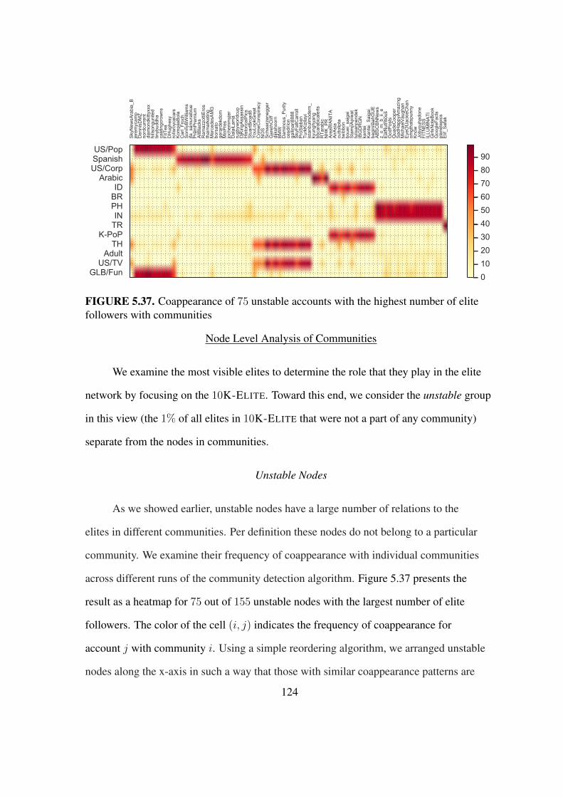
SkyN
ewsA
rabi
a_B
jere
myc
amp
Den
nisD
MZ
nord
curre
ntdi
amon
dkitt
yxxx
hills
ongu
nite
dtin
ybud
dha
cast
ingc
row
nsFi
tTea
DH
ughe
syro
llsro
ycec
ars
Kom
pasB
ola
Car
l_Fr
och
Sonn
yBW
illiam
sjfa
_sam
urai
blue
Prem
Prem
ium
AllB
lack
sR
amaz
zotti
Eros
thai
mar
ketin
gM
erce
desA
MG
bors
ato
gera
rdek
dom
Min
Pres
joch
emm
yjer
Dal
aiLa
ma
rugb
ywor
ldcu
pD
jKin
gAss
assi
nH
isto
rical
Pics
Stua
rtBro
ad8
YouL
ookG
reat
Crim
eCon
spira
cyN
OS
Schw
arze
negg
erG
aret
hClif
fdi
jksh
oorn
BMW
Dam
inou
s_Pu
rity
cesd
rilon
gallin
ari8
888
SkyF
allC
arro
llPr
oSie
ben
Turk
Kizi
layi
ista
nbul
mod
ern_
kyun
ghya
ngbb
cara
bica
lerts
RTa
rabi
cN
HK_
PRAr
eaW
ANIT
AAi
rAsi
acu
ttolip
tatw
ibbo
nbo
uei_
saig
aiSt
ampA
piw
attu
lisan
pend
ekIB
GD
RG
Nka
ntei
Kant
ei_S
aiga
ibe
gini
laah
GU
EAB
SCBN
New
sz_
o_m
_b_i
i_e
EatN
utrit
ious
God
Post
sQ
uade
Coo
per
SadH
appy
Amaz
ing
Mic
hael
Vaug
han
EyeO
fJac
kieC
han
omgt
hats
punn
yKn
owJo
byou
hado
neFl
TNES
SIL
LUM
lNAT
IG
irlsN
oteB
ook
Goo
gleF
acts
plan
etep
ics
Elif_
Safa
k
US/PopSpanishUS/Corp
ArabicID
BRPHIN
TRK-PoP
THAdult
US/TVGLB/Fun 0
102030405060708090
FIGURE 5.37. Coappearance of 75 unstable accounts with the highest number of elitefollowers with communities
Node Level Analysis of Communities
We examine the most visible elites to determine the role that they play in the elite
network by focusing on the 10K-ELITE. Toward this end, we consider the unstable group
in this view (the 1% of all elites in 10K-ELITE that were not a part of any community)
separate from the nodes in communities.
Unstable Nodes
As we showed earlier, unstable nodes have a large number of relations to the
elites in different communities. Per definition these nodes do not belong to a particular
community. We examine their frequency of coappearance with individual communities
across different runs of the community detection algorithm. Figure 5.37 presents the
result as a heatmap for 75 out of 155 unstable nodes with the largest number of elite
followers. The color of the cell (i, j) indicates the frequency of coappearance for
account j with community i. Using a simple reordering algorithm, we arranged unstable
nodes along the x-axis in such a way that those with similar coappearance patterns are
124

closer. We emphasize that the sum of the values in each row is not necessarily 100%,
because a node may coappear with more than one resilient community in each run of
the community detection. We recall that the higher the frequency of coappearance of a
node and a community suggests a tighter coupling between them. In fact, a node that
frequently coappears with two (or more) communities could be viewed as a (overlapping)
member of those communities which was disconnected from the communities due to
our strict coappearance requirement in forming resilient communities. Therefore, this
analysis illustrates how the set of unstable nodes can be further divided in accordance
with the coupling with the resilient communities. As the figure shows, there are a few
distinct coappearance patterns among nodes in Figure 5.37. These patterns are in fact
aligned with inter-community couplings in Figure 5.36(b), i.e. groups of communities
that have many unstable nodes coappearing with them have high coupling as well. A
few examples of these patterns are as follows: (i) A group of unstable nodes mostly
coappears with US/Pop and Global/Fun communities. The manual inspection of these
accounts shows that they are associated with less popular US-based accounts with various
foci. (ii) Another group of unstable nodes mostly coappears with the Spanish speaking
community and has a lower level of coupling with any other community. The users in this
set are mostly sport-related but not necessarily Spanish speaking, such as @rugbyworldcup,
@StuartBroad8, and @AllBlacks. (iii) The figure also shows that a group of unstable users
coappears with the ID and the K-Pop communities. Although the direct interconnection
between the two communities is low (as shown in Figure 5.36(a)) and the communities
do not seem to be contextually similar when compared to other communities, unstable
nodes in this group are tightly coupled with both communities and seem to be a part of
both communities. Users in this group include a few Asian online celebrities.
125

Uns
tabl
e
US/
Pop
Span
ish
US/
Cor
p
Arab
ic ID BR PH IN TR
K-Po
P TH
Adul
t
US/
TV
GLB
/Fun
Resilient Community
0
2
4
6
8
10
12
14
Num
ber o
f Ext
erna
l Com
mun
ities
IncomingOutgoing
FIGURE 5.38. Distribution of the number of related communities for nodes incommunities in the 10K-ELITE
Accounts that Connect Communities
Since individual communities contain related accounts, one natural question is “Do
specific nodes act as bridges to/from other communities?” In general, our analysis shows
that almost all users in the 10K-ELITE have at least one external incoming or outgoing
connection to a community other than their own. To answer this question, we make a
distinction between incoming (inBr(C)) and outgoing (outBr(C)) bridge node(s) for
community C that have incoming/outgoing connections from/to users in the largest
number of other unique communities. In other words, we measure the importance of a
bridge node based on the number of unique communities that it connects to rather than
the actual number of connections to other communities. For example, if node n1 has
1 000 external followers (i.e. followers in other communities) that are all located in two
communities and node n2 has 100 external followers that spread across 10 communities,
we consider n2 to be an outBr(C) as it is visible among a larger number of communities.
126

TABLE 11. The accounts that act as in/out bridges in each community.
Community inBr(s) outBr(s)
US/Pop 6BillionPeople, JonahLupton, p0tcomkatyperry, justinbieber, rihanna, ladygaga,ArianaGrande, aliciakeys, NICKIMINAJ,
kanyewest, ParisHilton, rickygervaisSpanish HalfordisMe instagram, verifiedUS/Corp EnergyDrinkRen twitter, HuffingtonPost, Support
Arabic KavalonThatsMe benlandis, paulatooths, TheGodLight, AxelKoster,neoseol, sodan4
ID fadjroeL UberSoc, echofonBR drangelocarbone KAKA, neymarjr, giseleofficialPH itsmovies, Drrake Earth PicsIN LeBronJames, LordLouis3 GreatestQuotes, LordLouis3, Brilliant Ads
TR Doarutkay, hidoturkoglu15, ertemsener, omerrcelik RT Erdogan, cbabdullahgul, Ahmet Davutoglu,memetsimsek, TurkishAirlines
K-PoP siwon407, jucklee TwitBirdTH Woodytalk Woodytalk
Adult Hot Girls 247, nlpantyhose, SexyCreeps gspot1177US/TV yokoono, shwood yokoono, MarthaStewart
GLB/Fun History Pics History Pics
Figure 5.38 presents the summary distribution of the number of unique external
communities for elites in each community. In essence, the boxplots of Figure 5.38
illustrate how many other elite communities the users in each community of elites
generally pay attention to (i.e. have in-edge or follow) and receive attention from
(i.e. have out-edge or being followed by), respectively. As the figure shows, users in
most communities are following a less diverse set of elites, compared to the variation
of the elites that are following them. On average, elites pay attention to 1-5 other
communities, but receive attention from 2-8 communities. The Arabic speaking and the
Thai communities are exceptions, because their set of friends are more diverse than the
followers. On one hand, users in Arabic speaking and US/TV communities follow the
most diverse set of other elites. On the other hand, elites in US/TV and Global/Fun have
the most diverse set of followers. There are a few outliers in most communities (shown
as stars) that have friends and followers in almost all communities. Per our definition,
these outliers act as an incoming/outgoing bridge for each community from/to external
communities in the elite network.
127

We individually examine these bridging accounts and their social contexts. Table 11
presents the usernames of the accounts in each community that have followers and friends
in the largest number of other communities as inBr and outBr for their community.
We observe that most of the outBr are well-recognized and popular individuals/entities
with appeal across diverse groups. However, the inBr are either not recognizable or are
genuinely interested in many different groups. We examine whether inBr/outBr are
different from the users in each community who have the largest in/out degrees. Indeed,
the users with the largest number of in/out degrees are among the inBr and outBr in
most of communities, respectively. Inversely, in all communities, inBr/outBr are among
the top 5% accounts with the highest in/out degree in that community. We have also
examined the PageRank of the incoming and outgoing bridge nodes in Table 11 to see
whether these bridges are among the most central nodes in the elite network. In general,
there exists a positive correlation between the number of external communities that a node
connects with and the PageRanks centrality of the node, and the PageRank of outBr are
higher than the rest of the nodes.
In summary, the analysis of social and community footprints along with the
identification of accounts in each community reveals cohesion among users in each
community around themes that are obvious in some cases (e.g. language, region, country,
business) and more subtle in other cases. The observed cohesion in these communities
indicates that they represent meaningful elements of the elite network. As we extend
the elite network, the number of communities could change. However, there is a clear
relationship among communities in different views as these related communities represent
the evolving view of a group of nodes with a specific and slowly changing social theme.
The inter-community connectivity and coupling can be used to create coarse views of the
topology of the elite network. These coarse summary views capture the interest among
128

communities and community hierarchies, respectively. Finally, the analysis at the node
level either among nodes inside a community or unstable nodes reveals the nodes that
are bridging a community to other communities or reside at the boundary of two or more
communities.
Tracing Elite Communities in the Entire Social Graph
As we mentioned earlier, the identified communities in the elite network only
reveal the modular structure of friendships among elites, and therefore the communities
of regular users could hypothetically be very different from communities of the elite
network. Our goal in this section is to check “whether the communities detected in the
elite network provide any insight about the topological structure of the entire graph.” Our
analysis is in part motivated by the observation that many communities remain effectively
the same as the elite network is extended in its size, as provided earlier in this section.
Since it is impossible for us to capture the full social graph of Twitter, our methodology
uses a random sample of Twitter users and traces the existence of modular structures
using the communities identified among elites. To this end, we use communities of elites
in particular as landmarks for an interest-based clustering of regular users.
Landmark Clustering Using the Elite Communities
As we showed earlier in Figure 5.27, 80% of the regular users follow at least one
elite in the 10K-ELITE. Given the high reach of the elites in this view, it seems natural
to use them as landmarks to classify regular users based on the elites that they follow.
Figure 5.39 presents a detailed view of the elite friends of the 10K+ regular randomly
sampled Twitter users. In each plot we group the regular users on the x-axis based on the
number of elite friends (elites that the sample user follows). Figure 5.39(a) presents the
129

1 2 3 4 5 6 7 8 9Regular Users Grouped by the Num. Elite Friends: 2n
0
2
4
6
8
10
Com
mun
ities
of E
lite
Frie
nds
(a) Distribution of number of elitecommunities that a regular user follows
1 2 3 4 5 6 7 8 9Regular Users Grouped by the Num. Elite Friends: 2n
20
30
40
50
60
70
80
90
100
Belo
ngin
g Fa
ctor
(b) Distribution of the belonging factor
FIGURE 5.39. Using elite communities as landmarks to cluster regular users.
summary distribution of the number of communities amongst the corresponding elite
friends. As the figure shows, each regular user follows elites that are in 1-8 different
communities. We use these elite communities as landmarks to cluster regular users. For
each regular user, we first compute a belonging vector that counts the fraction of its elite
friends that are in any community. A regular user is then mapped to the elite community
that makes up for the majority of its elite friends. Figure 5.39(b) shows the maximum
element in the belonging vector that we refer to as the belonging factor. As our results
demonstrate, the median belonging factor is at least 70%. Therefore, most regular users
can be confidently mapped to a single elite community.
We also examined the friend-follower relationships between regular users (edges)
with respect to the elite communities for approximately 100K edges. For each edge, we
map the friend and the follower to a community as previously explained and check if they
map to the same community. Our examination shows that 64.8% of the friend-follower
relationships are between users who map to the same community. Note that 69.1% of
relationships among elites are within the same community.
130

We conclude that the identified communities in the elite subgraph provide a
great set of landmarks for clustering regular users that follow the elites. Therefore,
via community detection on a very small portion of the social graph, namely the elite
network, we can effectively identify groups of tightly connected nodes in almost the entire
graph.
Influence Among Elites
In this section, we turn our attention to how the elites may influence other elites
on Twitter. Influence is a rather subtle effect of user u on other users that may not be
properly measured by a single metric. In the context of graph theory and complex
network analysis, various indicators of centrality have been proposed to measure the
importance of each node, e.g. the number of followers (out degree), betweenness,
closeness, or eigenvector centrality. Alternatively, historical measurements of a user’s
user in engaging an audience, such as the number of retweets, mentions, or comments
have also been used to quantify users’ influence. These measures of importance are in fact
correlated with the degree to which a user can influence others in the same network [97].
Prior studies on Twitter mention the subtleties in quantifying the influence and used
various metrics to capture different aspects of influence. Kwak et al. [163] used three
metrics – the number of followers, PageRank, and the number of retweets – and found
that the ranking of the most influential users differed depending on the metric. Cha et al.
[59] also compared three different measurements of influence – the number of followers,
retweets, and mentions – and reported that the most followed users did not necessarily
score high on the other metrics.
We consider the following two sources of information to measure the influence
of elite user u on other elites in the 10K-ELITE: (i) Social graph: The social
131

interconnections captured in the elite network help us measure the centrality of a user’s
topological position within that network. (ii) User engagement: The success of an elite
in engaging others also serves as a resource to measure influence. Specifically, we use
interactions in the form of retweet and reply in our analysis.
Our objective in this work is slightly different than those of the prior studies, since
our focus is to capture the influence of elites on each other and not the regular users in the
OSN. Hence, we extend or modify the formerly introduced measurements of influence
as needed. For instance, we do not use metrics such as the total number of retweets or
favorites of a user’s tweet, since they cannot be broken down by the regular or the elite
users who contributed to those numbers. We also do not intend to reconstruct the actual
diffusion tree which may contain regular users. Therefore we specifically focus on the
engagement-based influence regardless of its diffusion. With respect to indices that
are based on user engagement, we extend the commonly used metrics (e.g. number of
retweets) and consider the number of unique users that engage with the influencer as well.
Next, we describe how we identify the most influential elites using each one of
these data sources, and then examine the overlap among influential users based on each
metric.
Social Graph
The most primitive measure of influence captured through the elite subgraph is
the user popularity, i.e. the number of elite followers. In the context of the social graph,
popularity translates to the node out-degree. It is important to remember that since tweets
cascade through the system, the number of followers alone does not reflect the influence
comprehensively. More sophisticated measures such as PageRank [46] are used to better
capture propagation of influence along the network.
132

106 107 108
Num. Followers
101
102
103
104
Num
. Elit
e Fo
llow
ers instagram
mikeyk
BarackObama
PontifexPontifex_es
Pontifex_ptPontifex_it
nytimes
jimmyfallon
0.0008
0.0016
0.0024
0.0032
0.0040
0.0048
0.0056
0.0064
Page
Ran
k
FIGURE 5.40. Visualizing centrality captured through the social graph.
The PageRank of a node measures its centrality in the network by showing its
relative reachability to other nodes. PageRank is essentially a generalization of degree
centrality and is correlated with the number of nodes that can be reached from the node
by different paths. However, the contributions of faraway nodes are penalized as the
length of the paths increase. In the elite network, PageRank translates to how easily a
tweet by an elite reaches (and influences) other elites. We compute the PageRanks of
nodes in the 10K-ELITE to measure their centrality. A key question is “whether (and
to what extent) the PageRank of a node is correlated with its number of followers and
elite followers (i.e. the out-degree in the entire network and the out-degree in the elite
network)?” To explore this issue, Figure 5.40 presents the number of followers (on the
x axis), number of elite followers (on the y axis), and the PageRank (as the size and the
color of circles) for all elites in the 10K-ELITE using a log scale for both axes. We also
labeled 10 accounts with the highest PageRank values in this figure. We observe a few
interesting points in this figure. First, the figure shows a high correlation between the
number of followers and the number of elite followers. Second, we observe that many
133

accounts with the highest PageRanks have indeed a large number of followers and elite
followers (notice the top right corner of the figure). However, it is interesting that some
users (e.g. all Pope Francis’s accounts) whose number of (elite) followers are an order
of magnitude smaller than the maximum number of (elite) followers, still achieve some
of the highest PageRanks. An example of such a case in the figure is @mikeyk, the co-
founder and CTO of Instagram, that has the second highest PageRank despite having a
small number of regular and elite followers. Our hypothesis is that his high PageRank is
due to his close tie to @instagram (Instagram’s official account on Twitter), which has the
highest PageRank. To test this hypothesis, we remove instagram from the elite network,
which leads to the drop of mikeyk’s PageRank to rank 3 288, hence our hypothesis is
correct.
Social Engagement: Reply & Retweet
The number of reactions to a certain tweet is a measure of the tweet’s popularity
and in turn the popularity of the user who posted it. Prior studies have used retweets
to measure influence among Twitter users [59, 163, 30, 60]. They mostly use the
total number of retweets for all tweets posted by a user to measure her influence [59].
Calculating PageRank over the retweet graph has also been proposed a metric to measure
influence [267]. The main difficulty in using this method is the way Twitter organizes the
retweets; for each retweet by user ux, Twitter indicates the identifier of the corresponding
original tweet and the user uorig that posted the original tweet. Therefore, the intermediate
users involved in the diffusion of a tweet are obscured. To tackle this limitation, some
studies proposed techniques to reconstruct the diffusion tree and compute the PageRank
on the diffusion construct. All these measures, however, count the users under influence
as equal and cannot distinguish influence on elite and regular users.
134

Our proposal is to measure pairwise influence of elites on each other and then
aggregate those measurements. In addition to using retweets, we also use replies as they
provide a measure of an elite’s capability to trigger a reaction in other elites. Our dataset
contains more than 31M tweets from the accounts in 10K-ELITE. 6.5M of these tweets
are retweets and 5M are replies.
We capture the overall influence of user u (in terms of retweet or reply) on all other
elites with the following three metrics: (i) Number of reactions is the total number of
retweets (or replies) of original tweets posted by u that is captured in our dataset. Note
that this metric is a simple extension of the number of retweets used in prior studies to
identify key influential users that counts all the reactions, not just those by the elites. (ii)
Number of influenced elites is the number of unique elites that have retweeted (or replied
to) at least one of u’s original tweets. (iii) Aggregate influence of user u is the summation
of the fractions of any other elites’ captured tweets that is a retweet of (or is a reply to)
tweets originally generated by u. More specifically:
Aggregate Influence(u) =∑
v∈Elite
RTu→vNv
(5.1)
where RTu→v and Nv denote the number of times that user v retweeted (or replied to)
user u and Nv is the total number of v’s tweets.
Figure 5.41 shows a three-dimensional measure of retweet and reply influence for
users in the 10K-ELITE as scattered plots. Each circle in Figure 5.41(a) (Figure 5.41(b))
represents a single elite u where its x coordinate indicates the total number of retweet
(reply) by other elites, and its y coordinate shows u’s aggregate retweet (reply) influence.
We also encode the number of influenced elites by each user in both the size and the color
of each circle. Additionally, we labeled some of the key circles with the name of their
corresponding user. Figure 5.41(a) illustrates a few interesting points: First we observe
135
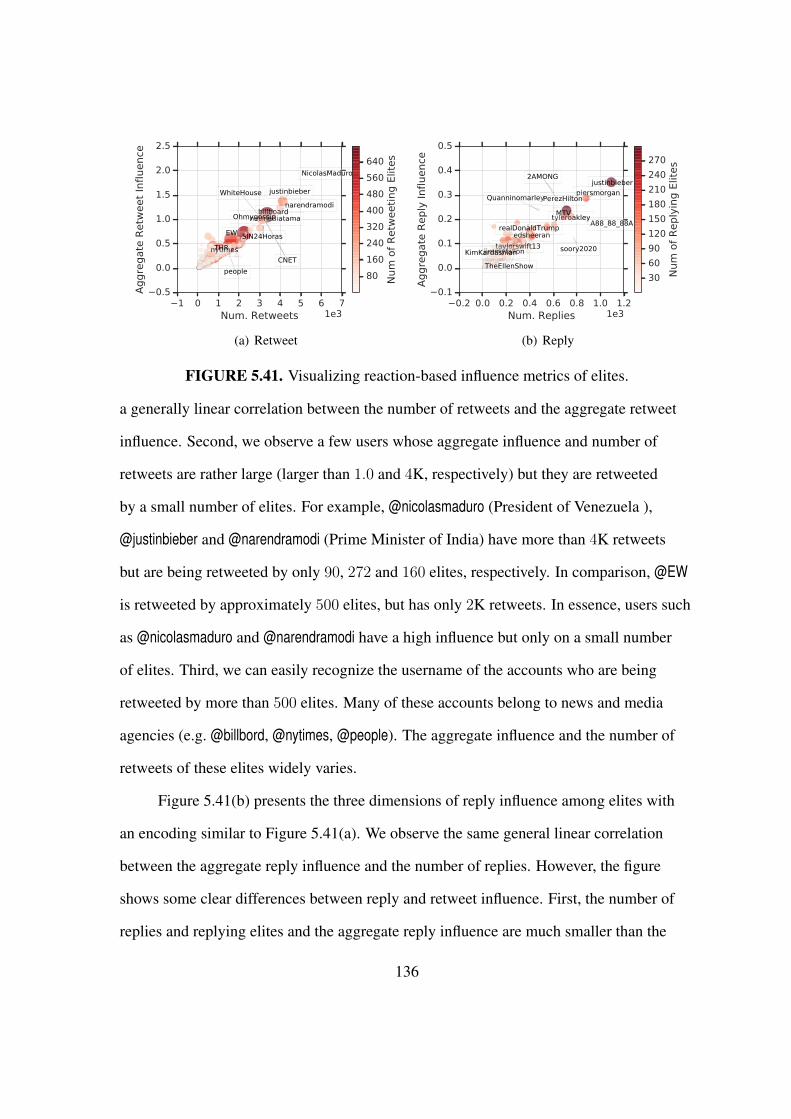
1 0 1 2 3 4 5 6 7Num. Retweets 1e3
0.5
0.0
0.5
1.0
1.5
2.0
2.5A
ggre
gate
Retw
eet
Influence
NicolasMaduro
justinbieber
narendramodi
netmediatamabillboard
CNET
SIN24Horas
Ohmygossip
WhiteHouse
EW
nytimes
people
THR
80
160
240
320
400
480
560
640
Num
of
Retw
eeti
ng E
lites
(a) Retweet
0.2 0.0 0.2 0.4 0.6 0.8 1.0 1.2Num. Replies 1e3
0.1
0.0
0.1
0.2
0.3
0.4
0.5
Aggre
gate
Reply
Influence
justinbieber
A88_88_88A
piersmorgan
soory2020
tyleroakley
2AMONG
QuanninomarleyPerezHilton
TheEllenShow
taylorswift13
MTV
edsheeranrealDonaldTrump
jimmyfallonKimKardashian
30
60
90
120
150
180
210
240
270
Num
of
Reply
ing E
lites
(b) Reply
FIGURE 5.41. Visualizing reaction-based influence metrics of elites.
a generally linear correlation between the number of retweets and the aggregate retweet
influence. Second, we observe a few users whose aggregate influence and number of
retweets are rather large (larger than 1.0 and 4K, respectively) but they are retweeted
by a small number of elites. For example, @nicolasmaduro (President of Venezuela ),
@justinbieber and @narendramodi (Prime Minister of India) have more than 4K retweets
but are being retweeted by only 90, 272 and 160 elites, respectively. In comparison, @EW
is retweeted by approximately 500 elites, but has only 2K retweets. In essence, users such
as @nicolasmaduro and @narendramodi have a high influence but only on a small number
of elites. Third, we can easily recognize the username of the accounts who are being
retweeted by more than 500 elites. Many of these accounts belong to news and media
agencies (e.g. @billbord, @nytimes, @people). The aggregate influence and the number of
retweets of these elites widely varies.
Figure 5.41(b) presents the three dimensions of reply influence among elites with
an encoding similar to Figure 5.41(a). We observe the same general linear correlation
between the aggregate reply influence and the number of replies. However, the figure
shows some clear differences between reply and retweet influence. First, the number of
replies and replying elites and the aggregate reply influence are much smaller than the
136
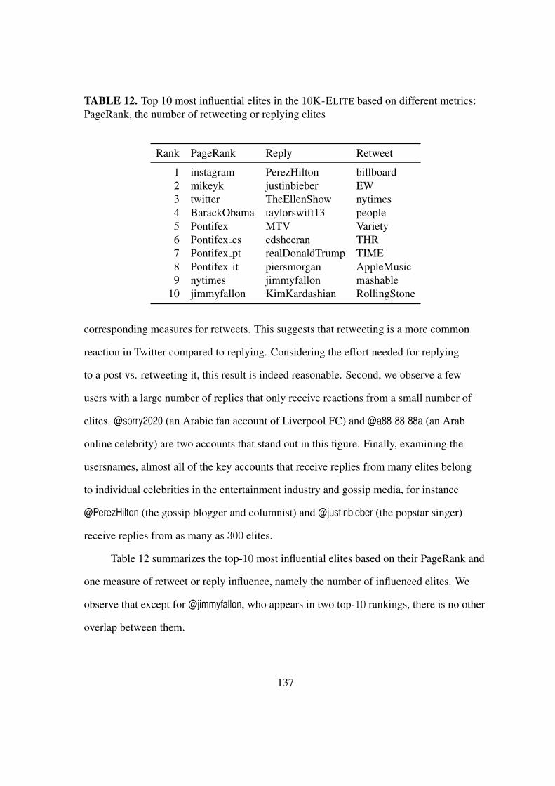
TABLE 12. Top 10 most influential elites in the 10K-ELITE based on different metrics:PageRank, the number of retweeting or replying elites
Rank PageRank Reply Retweet
1 instagram PerezHilton billboard2 mikeyk justinbieber EW3 twitter TheEllenShow nytimes4 BarackObama taylorswift13 people5 Pontifex MTV Variety6 Pontifex es edsheeran THR7 Pontifex pt realDonaldTrump TIME8 Pontifex it piersmorgan AppleMusic9 nytimes jimmyfallon mashable
10 jimmyfallon KimKardashian RollingStone
corresponding measures for retweets. This suggests that retweeting is a more common
reaction in Twitter compared to replying. Considering the effort needed for replying
to a post vs. retweeting it, this result is indeed reasonable. Second, we observe a few
users with a large number of replies that only receive reactions from a small number of
elites. @sorry2020 (an Arabic fan account of Liverpool FC) and @a88 88 88a (an Arab
online celebrity) are two accounts that stand out in this figure. Finally, examining the
usersnames, almost all of the key accounts that receive replies from many elites belong
to individual celebrities in the entertainment industry and gossip media, for instance
@PerezHilton (the gossip blogger and columnist) and @justinbieber (the popstar singer)
receive replies from as many as 300 elites.
Table 12 summarizes the top-10 most influential elites based on their PageRank and
one measure of retweet or reply influence, namely the number of influenced elites. We
observe that except for @jimmyfallon, who appears in two top-10 rankings, there is no other
overlap between them.
137

56% 72%12%
64%
20% 4%12%
reply retweet
PageRank
Top 25 most influential
(a) Ranked as top 25
47% 49%15%
47%
17% 15%21%
reply retweet
PageRank
Top 100 most influential
(b) Ranked as top 100
34% 34%16%
36%
14% 14%36%
reply retweet
PageRank
Top 1000 most influential
(c) Ranked as top 1K
FIGURE 5.42. Overlap among different influence measures
The observed minimal overlap among the top-10 most influential users based on
different measure raises the following question: “How does the overlap among the top-N
most influential users based on different metrics change with N?” Exploring this question
reveals the level of separation between the influential users according to each measure.
The three Venn diagrams in Figure 5.42 present pairwise and three-way overlap among
top-N influential users according to the three metrics for N equal to 25, 100 and 1K. We
observe that the 3-way overlap among different groups of influential users grows with N
from 12% to 21% and 36%. Interestingly, even for the top-1K, between 34-36% of users
are considered influential based on just a single metric, and the plots do not reveal any
similarity between ranking observed by any two metrics. Hence, each of these metrics
captures a different aspect of importance/influence, and the topological centrality of a
user’s position in the social graph does not lead to his success in attracting large reactions
from other elites. This finding is generally aligned with the lack of correlation in various
measurements of influence in prior studies [59, 163].
138
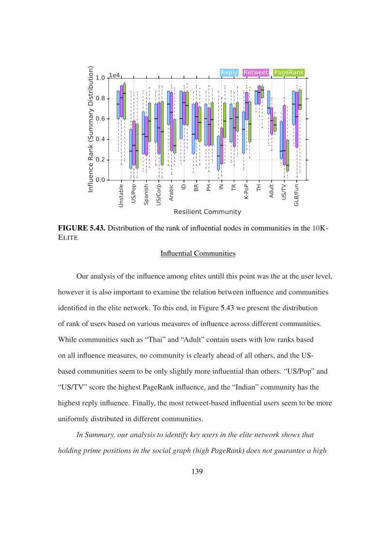
Unst
able
US/P
op
Spanis
h
US/C
orp
Ara
bic ID BR
PH IN TR
K-P
oP
TH
Adult
US/T
V
GLB
/Fun
Resilient Community
0.0
0.2
0.4
0.6
0.8
1.0
Influence
Rank
(Sum
mary
Dis
trib
uti
on)
1e4 Reply Retweet PageRank
FIGURE 5.43. Distribution of the rank of influential nodes in communities in the 10K-ELITE
Influential Communities
Our analysis of the influence among elites untill this point was the at the user level,
however it is also important to examine the relation between influence and communities
identified in the elite network. To this end, in Figure 5.43 we present the distribution
of rank of users based on various measures of influence across different communities.
While communities such as “Thai” and “Adult” contain users with low ranks based
on all influence measures, no community is clearly ahead of all others, and the US-
based communities seem to be only slightly more influential than others. “US/Pop” and
“US/TV” score the highest PageRank influence, and the “Indian” community has the
highest reply influence. Finally, the most retweet-based influential users seem to be more
uniformly distributed in different communities.
In Summary, our analysis to identify key users in the elite network shows that
holding prime positions in the social graph (high PageRank) does not guarantee a high
139

influence measured through retweet and reply. Users with the highest level of influence
captured via retweet are mostly related to news media and music industry, while those
who exhibit the highest level of reply influence are present with the entertainment gossip
media industries. Analyzing the distribution of influential users among communities, we
observe a couple of communities have disproportionately few influential users, and US-
based communities include the most influential ones.
Summary
In this chapter, we captured and analyzed the elite network of Twitter. We define
n-ELITE as the view of the elite network that contains all the friend-follower relationships
between the n most followed accounts in Twitter. We showed that the most popular elites
(accounts with the largest number of followers) are more central in the elite network, and
as the less popular elites are added to the network, they sit in outer layers of an “onion-
like” structure. We demonstrated that the followers of the 10K-ELITE comprise 80%
of the users in the entire OSN, and argued for limiting the size of this elite network
to the top 10K most followed accounts. We showed that the network is composed of
tightly connected communities with strong social cohesion. We unveiled the coarse
level structure of the elite network using these communities and identified at the user
level the accounts that sit at the overlapping boundaries of some communities. We also
demonstrated the potential usage of these communities as landmarks to cluster the OSN
by mapping a regular user to the community that contains the majority of the elites that
it follows. While 35% of the friend-follower relationships between elites fall across the
boundaries of different communities, the percentage of friend-follower relationships
between regular users that are mapped to different elite communities is 39%. Finally, we
assessed the aggregate influence of each elite on the rest of the elite network using three
140

different methods and explored the (dis)similarities among top-N influential users based
on various metrics. We plan to extend this work by investigating the temporal evolution of
the elite network along with its underlying causes and implications.
141

Part II
The Internet
142

CHAPTER VI
INTERNET TOPOLOGY MAPPING; TAXONOMY & TECHNIQUES
Capturing an accurate view of the Internet topology is of great interest to the
networking research community as it has many uses ranging from the design and
evaluation of new protocols and services to the vulnerability analysis of the network’s
infrastructure. However, the scale of today’s Internet coupled with its distributed and
heterogeneous nature makes it very challenging to acquire a complete and accurate
snapshot of the topology. The purpose of this survey is to examine the main research
studies that have been conducted on topics related to Internet topology discovery in the
last 15-20 years and present some of the main lessons learned from these past efforts.
To this end, we classify these prior studies according to the “resolution” or “level” of
the topology; that is, interface-level, router- level, PoP-level and AS-level. For each
resolution, we describe the main techniques and tools used for data collection, identify
their major limitations and issues, and discuss the key implications that these limitations
have on the quality of the collected data. In the process, we present the latest efforts
in modeling the Internet’s topology at the different levels and report on the role that
geographic characteristics play in this context. We present the lessons learned as a
checklist that every researcher working on Internet topology discovery-related problems
should consult to minimize the risk of repeating some of the same or similar mistakes that
have been made in the past and as a result have hampered progress in this important area
of Internet research.
143

Introduction
Composed of approximately 50 000 networks or Autonomous Systems (AS), the
Internet reigns as the ultimate network of networks. Most of these networks are separately
owned and managed (however companies that own and manage multiple ASes do
exist [50]), cover different geographic areas, build their own physical infrastructures, and
serve different purposes. For example, an AS can be a Network Service Provider (NSP),
an Internet Service Provider (ISP), an education network, a Content Provider (CP),
a Content Distribution Network (CDN) or can provide any combination of these or
other services. The diversity in network type and business along with their autonomous
management makes it clear why individual ASes use network equipment from different
vendors to build and operate different infrastructures, possibly with greatly varying
physical topologies and why, in turn, not all ASes deploy the same intra-domain routing
protocol but instead use the one(s) that best support(s) their operational needs. It also
explains why one of the critical features of the Border Gateway Protocol (BGP) is its
expressiveness – the ability to let ASes with potentially competing business interests
express different policies for interconnecting with one another, presumably for the
purpose of enabling the smooth and economically viable exchange of traffic.
As a result of this diversity, its scale, and its distributed and heterogeneous
nature, mapping the Internet’s global topology is inherently difficult and enormously
challenging. For one, since the decommissioning of the NSFNET [189], there exists
no entity or organization that has a complete picture (i.e., “ground truth”) of the entire
Internet or its individual constituents or ASes. Moreover, there exists no protocol or
service whose sole purpose is the discovery of the network topology[223, 202]. In
fact, the measurement tools that are most often used for topology discovery are merely
“engineering hacks” that researchers have proposed to collect information about the
144

Internet topology. In particular, the two most commonly used techniques for topology
discovery, namely traceroute and BGP, have originally been designed for entirely different
purposes – traceroute as originally introduced by V. Jacobson is a network debugging tool
[253, 282, 23] and BGP is the de-facto standard inter-domain routing protocols in today’s
global Internet that indicates reachability rather than connectivity of individual ASes [49].
These difficulties and challenges notwithstanding, the study of the Internet’s
topology has fascinated both networking and non-networking researchers for the last 15-
20 years. While non-networking researchers view the Internet or its topology as a prime
example of a complex and large-scale technological network and are mainly interested
in studying its structural properties and predicting its behavior, the network research
community’s interest is in general motivated by more practical concerns. For example,
various topological properties of the Internet affect the performance of network protocols,
network applications and services. Thus, a better understanding of the Internet topology
and its main characteristics would enable network researchers to design better network
protocols or services and evaluate them under more realistic conditions. Moreover, an
accurate map of the Internet would be very helpful for network engineers and operators
who are constantly trying to improve or optimize the allocation of network resources such
as proxies, replica servers, and data centers. Similarly, having a detailed and complete
map of the Internet’s topology, preferably annotated with attributes such as the exact
geographic location of certain network equipment, could inform the study of a wide
range of security-related problems and protocols such as backtracking malicious traffic
or assessing the vulnerability of the Internet to blackouts or attacks on parts of its physical
infrastructure.
The purpose of this survey is twofold. First, by viewing the Internet’s topology
at different well-defined resolutions or levels of detail (i.e., interface-level, router-level,
145

Point-of-Presence or PoP-level, and AS-level), we present a systematic assessment of
the main studies that have dealt with measuring and/or modeling the Internet’s topology
and have been published in the last 15-20 years. Second, by describing in detail the data
collection techniques and tools, types of collected datasets, and inference methods used in
these different studies, we provide a checklist that every researcher interested in working
on Internet topology-related problems should consult before using these tools, datasets,
or methods in their own work. Importantly, this checklist collects in one place our current
understanding of the main limitations that these tools, datasets or methods have when
used in the context of Internet topology research. In a nutshell, by being aware of these
limitations and understanding their root causes, researchers will be able to answer for
themselves whether or not the used tools, datasets, or methods are of sufficient quality to
successfully tackle the particular research problem they are interested in. In this sense,
this survey reports on lessons learned from 15-20 years of Internet topology research
that will hopefully prevent researchers from repeating some of the same or similar
mistakes that have been made in the past and that have negatively impacted progress in
this important area of networking research.
The rest of this survey is organized as follows: Section 6.2 presents the notion of
different Internet topology resolutions which defines our taxonomy. Sections 6.3, 6.4,
6.5, and 6.6 cover Internet topology at interface-level, router-level, PoP-level, and AS-
level, respectively. In each section, we discuss the main data collection techniques and
tools, types of collected datasets, and inference methods that have been used to study the
topology at the corresponding resolution. We conclude our survey in Section 6.8 with a
discussion of the main lessons learned and mention some of the exciting open research
problems that will require new and creative solution methods.
146
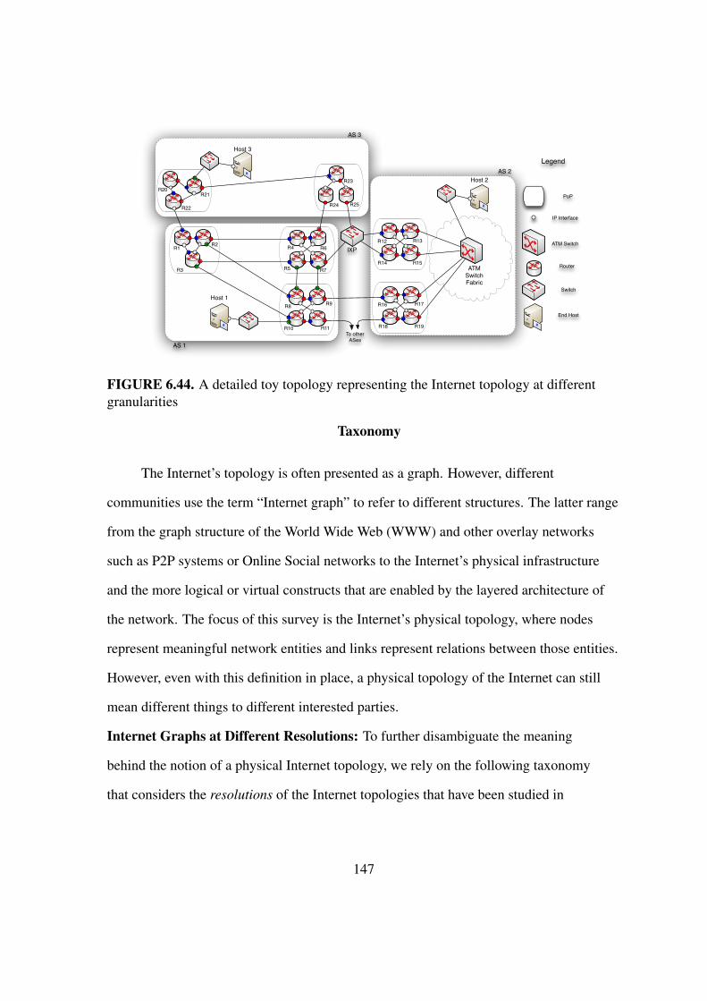
IXP
Host 1
Host 3
ATM SwitchFabric
AS 1
AS 2
AS 3
Host 2
R1 R4R2
R3
R9
R6
R5 R7
R11R10
R8
R12
R14
R13
R15
R16
R18
R17
R19
R20
R22
R21
R24
R23
R25
ATM Switch
Router
Switch
End Host
Legend
IP Interface
To other ASes
PoP
FIGURE 6.44. A detailed toy topology representing the Internet topology at differentgranularities
Taxonomy
The Internet’s topology is often presented as a graph. However, different
communities use the term “Internet graph” to refer to different structures. The latter range
from the graph structure of the World Wide Web (WWW) and other overlay networks
such as P2P systems or Online Social networks to the Internet’s physical infrastructure
and the more logical or virtual constructs that are enabled by the layered architecture of
the network. The focus of this survey is the Internet’s physical topology, where nodes
represent meaningful network entities and links represent relations between those entities.
However, even with this definition in place, a physical topology of the Internet can still
mean different things to different interested parties.
Internet Graphs at Different Resolutions: To further disambiguate the meaning
behind the notion of a physical Internet topology, we rely on the following taxonomy
that considers the resolutions of the Internet topologies that have been studied in
147

the past [223, 45, 283, 91]. In particular, we view Internet topology at four different
granularity or resolution levels, organized from finest to coarsest as follows:
I) Interface level: At this level, a node represents a network interface with a
designated IP address. An interface belongs to a host or a router and there is a one-to-one
mapping between nodes and IPs [231, 177]. At the same time, a link between two nodes
shows a direct network layer connectivity between them. This implies that the topology
at this level ignores devices functioning at OSI layers lower than the network or IP layer
(e.g. hubs and switches).
II) Router level: The topology at this level is often the result of grouping interfaces
that belong to the same router [244]. At this level, a node represents an IP-compliant
network device (e.g. a host or a router with multiple interfaces). Two nodes are connected
by an edge if the corresponding devices have interfaces that are on the same IP broadcast
domain.
III) PoP level: A PoP (Point of Presence) is a concentration of routers that belong
to the same AS [104, 279]. ASes commonly build their physical networks in a more or
less pronounced hierarchical manner; that is, an AS’s PoPs are interconnected to form the
AS’s “backbone” and are also the locations where the AS connects to the PoPs of other
ASes [271] and where it provides access to its customers or end users. In this sense, a
node in the topology at this level represents a PoP that belongs to an AS. A link between
two PoPs indicates that there is physical connectivity between the routers of the two PoPs.
IV) AS level: As opposed to the previous constructs, the AS-level topology
represents a more logical view of the Internet [181, 87]. A node at this level represents
an AS identified by a 16-bit (recently also a 32-bit) AS number. A link in the AS-level
topology represents a business relationship between two ASes. Theses relationships
reflect who pays whom when traffic is exchanged between the ASes in question and
148

are key to a properly functioning and financially viable Internet ecosystem [223, 188].
Traditionally, these relationships are categorized into a) customer-provider (C2P), b) peer-
peer (P2P), and c) sibling relationships, but other forms of relationships are known to
exist as well. Since ASes typically cover entire geographic regions, with different PoPs
in those regions’ major cities, the physical connectivity between two ASes that have an
established business relationship often occurs at multiple locations. Thus, an AS link is
virtual rather than physical in nature in the sense that it is an abstraction and typically
represents multiple physical connections between the two ASes [264].
In this survey, we make use of this taxonomy to categorize prior Internet topology
studies. Moreover, for the different studies concerned with one and the same resolution,
we (i) provide a detailed assessment of the limitations of the techniques employed to
collect data, as well as an assessment of the quality of the collected data that is used
to study the topology at the given resolution, and (ii) carefully examine the geographic
characteristics of the inferred topology and the extent to which the topology at the given
resolution is annotated with geographic attributes.
Figure 6.44 shows three resolutions of the topology. At the finest level, the
router-topology is presented. The PoP-level topology is generated when PoPs and the
connections between them are considered. Finally, the AS-level topology is obtained
when we look only at the ASes and the links between them.
Data Types and Data Collection: The nature of the data and the type of data collection
techniques are two other elements that we use to classify prior Internet topology studies.
Regarding the nature of the collected data, measurements can be performed in the control
plane or the data plane. In terms of measurements performed in the control plane, the
collected data reveals information about routing in the Internet. For instance, BGP tables
store the AS paths to reach different prefixes and they are classic examples of control
149

plane data. In contrast, data plane measurements aim to discover the actual paths that
packets travel along. The simplest measurement of this form is Ping. It measures the
reachability of a target IP address and also reports the Round Trip Time (RTT) between
the target IP and a source, based on the route that the probe packets take in the Internet.
Regarding the collection technique, a measurement can be either active or passive. In
active measurements, actual packets (i.e. probe messages) are sent into the network and
the replies are collected. On the other hand, passive measurements only tap into a wire
and collect the information that is already flowing over that wire. traceroute and BGP
monitors are examples of active and passive measurement techniques, respectively. A list
of commonly-employed data sources and measurement techniques used for studying the
Internet topology at each resolution is provided in Table 13.
Geographic Attributes of The Topology: Although a main element of a topology is
connectivity, geography is another element that, when appropriate, can be added to the
topology to increase its usability. However, the definition of a geographically annotated
topology depends on the different resolutions of the Internet topology. Interfaces, routers
and PoPs are entities that can in theory be geographically mapped to an exact location on
a map. A geographical Internet map at these three levels of resolution involves assigning
a pair of longitude and latitude coordinates to each entity. Therefore, the topology graph
consists of points on the map and the links that connect those points together.
However, in the case of the AS-level topology, geography is a more subtle notion
and typically refers to the geographic region covered by an AS. In such a view, an AS
is shown as a colored area on a map that represents its coverage, and different ASes
covering parts of that same region are stacked vertically and are shown in different colors.
In such a representation, AS relationships can be represented by connections between
the differently-colored regions and can be further refined by incorporating the ASes’
150

TABLE 13. Different resolutions of Internet topology and the commonly used datasources to capture the topology in addition to the corresponding limitations andchallenges
Resolution Tools & techniques Limitations & challengesInterface-level traceroute Router response inconsistency
Opaque Layer 2 cloudsLoad balance routersProbe message filtering
Subnet discovery Router response inconsistencyProbe message filtering
Router-level Alias Resolution ScalabilityInaccurate (false positive and false negative)
SNMP Only applicable to one ASRequires administrative authorities over theAS
MRINFO Only applicable to ASes with DVMRPmulticast-ready routers
Aggregation techniques Mapping IP to Geo is inaccurateDNS name to Geo is not always applicableDNS misnaming can add more error
Delay based techniques Sensitive to knowledge of geography andplacement of candidate PoPs
Online data sources Public online data is not always up-to-dateAS level BGP Reachability announcement protocol with
built in information hidingtraceroute Mapping IP to AS number is not trivial
Using private IPs and other interface levelinconsistencies add more complexities
Internet Routing Registries Obsolete data
PoPs and showing the inter-AS connections at the PoP-level. This picture is further
complicated by the existence of Internet eXchange Points (IXP), where multiple networks
connect at one (or a few close-by) physical locations through a multipoint connection.
As a result, the complete geo-annotated AS-level topology should be viewed as a hyper-
graph [223] where nodes cover areas and links are annotated by the locations of the their
corresponding PoPs.
151
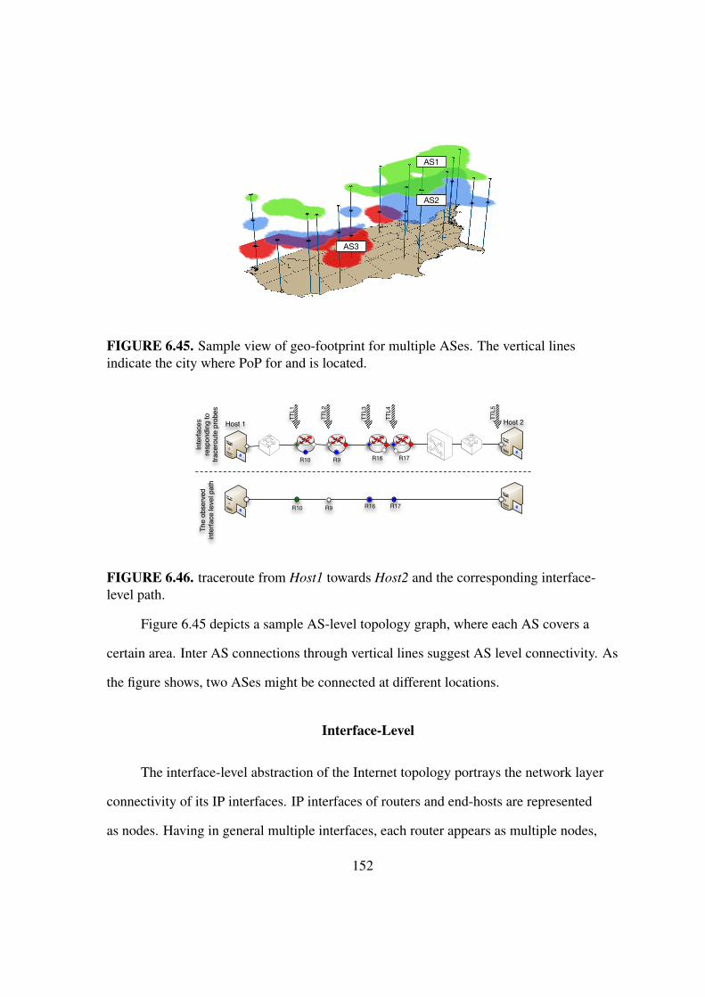
AS1
AS3
AS2
AS1
FIGURE 6.45. Sample view of geo-footprint for multiple ASes. The vertical linesindicate the city where PoP for and is located.
Host 1 Host 2
R9R10 R16 R17
TTL1
TTL2
TTL3
TTL4
R9R10 R16 R17
Inte
rface
s re
spon
ding
to
trace
rout
e pr
obes
TTL5
The
obse
rved
in
terfa
ce le
vel p
ath
FIGURE 6.46. traceroute from Host1 towards Host2 and the corresponding interface-level path.
Figure 6.45 depicts a sample AS-level topology graph, where each AS covers a
certain area. Inter AS connections through vertical lines suggest AS level connectivity. As
the figure shows, two ASes might be connected at different locations.
Interface-Level
The interface-level abstraction of the Internet topology portrays the network layer
connectivity of its IP interfaces. IP interfaces of routers and end-hosts are represented
as nodes. Having in general multiple interfaces, each router appears as multiple nodes,
152

while normal end-hosts with one interface are depicted as a single node. The topology
is typically simplified by ignoring end-hosts, therefore nodes only represent router
interfaces. Links represent direct network layer connectivity between nodes. However,
not all these links are point-to-point. For instance, layer 1 and layer 2 clouds can be
traversed, although the connectivity is represented as a single link.
traceroute is the most widely used tool to map the topology of the Internet at this
resolution. Based on the nature of the technique and the type of data it produces, it is an
active measurement method performed in the data plane [49, 39]. It uses limited Time-To-
Live (TTL) probes. The traceroute probes launched from a source to a target successively
discover the IP addresses of IP-compliant router interfaces along the forward path, and at
each hop measured RRT values are also reported. Multiple probe messages with the same
TTL can be used to discover the IP at the same hop. In the perfect scenario, probes for the
same hop would initiate a response from the same IP, but each would produce a slightly
different RTT due to the inherently dynamic nature of network traffic. In the rest of this
survey we assume that a single probe message is used for each hop discovery. Figure 6.46
shows the conducted traceroute from Host1 to Host2 and the observed interface-level
path. Only one IP address per hop is identified, and the result does not indicate any layer
2 infrastructures.
Each individual traceroute measurement reveals one IP path composed of multiple
IP segments. To discover the topology at the interface-level, the outcome of many
traceroute measurements should be merged. traceroute-based techniques require a
number of traceroute capable hosts (vantage points), and a list of target IPs. During a
measurement campaign, a set of vantage points launch traceroute probes towards a given
set of targets. The overall observed interface-level topology is generated from the union
of all the IP paths, each measured by a traceroute.
153
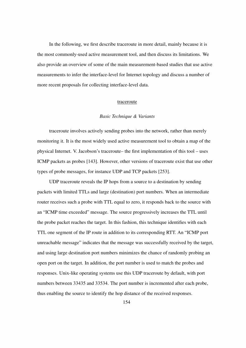
In the following, we first describe traceroute in more detail, mainly because it is
the most commonly-used active measurement tool, and then discuss its limitations. We
also provide an overview of some of the main measurement-based studies that use active
measurements to infer the interface-level for Internet topology and discuss a number of
more recent proposals for collecting interface-level data.
traceroute
Basic Technique & Variants
traceroute involves actively sending probes into the network, rather than merely
monitoring it. It is the most widely used active measurement tool to obtain a map of the
physical Internet. V. Jacobson’s traceroute– the first implementation of this tool – uses
ICMP packets as probes [143]. However, other versions of traceroute exist that use other
types of probe messages, for instance UDP and TCP packets [253].
UDP traceroute reveals the IP hops from a source to a destination by sending
packets with limited TTLs and large (destination) port numbers. When an intermediate
router receives such a probe with TTL equal to zero, it responds back to the source with
an “ICMP time exceeded” message. The source progressively increases the TTL until
the probe packet reaches the target. In this fashion, this technique identifies with each
TTL one segment of the IP route in addition to its corresponding RTT. An “ICMP port
unreachable message” indicates that the message was successfully received by the target,
and using large destination port numbers minimizes the chance of randomly probing an
open port on the target. In addition, the port number is used to match the probes and
responses. Unix-like operating systems use this UDP traceroute by default, with port
numbers between 33435 and 33534. The port number is incremented after each probe,
thus enabling the source to identify the hop distance of the received responses.
154
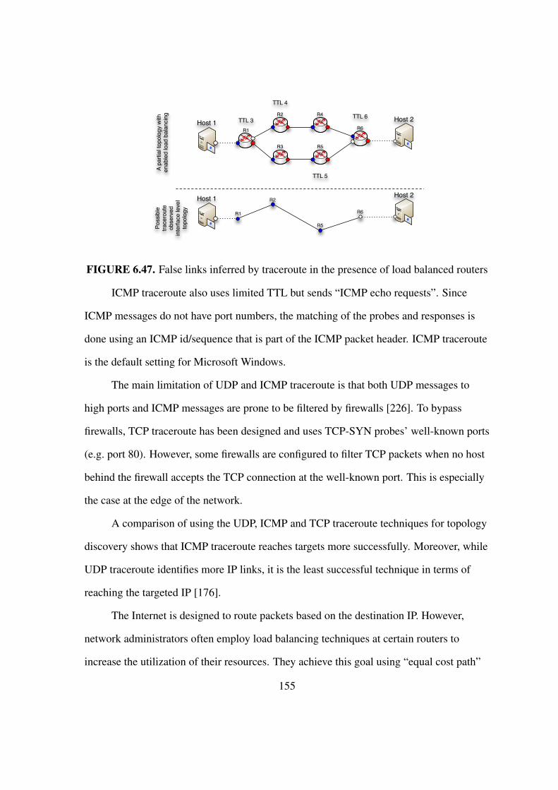
Host 2Host 1 TTL 3
TTL 4
TTL 5
TTL 6
R1
R2
R3
R4
R5
R6
Host 2Host 1
R1
R2
R5
R6
A pa
rtial
topo
logy
with
en
able
d lo
ad b
alan
cing
Poss
ible
tra
cero
ute
obse
rved
in
terfa
ce le
vel
topo
logy
FIGURE 6.47. False links inferred by traceroute in the presence of load balanced routers
ICMP traceroute also uses limited TTL but sends “ICMP echo requests”. Since
ICMP messages do not have port numbers, the matching of the probes and responses is
done using an ICMP id/sequence that is part of the ICMP packet header. ICMP traceroute
is the default setting for Microsoft Windows.
The main limitation of UDP and ICMP traceroute is that both UDP messages to
high ports and ICMP messages are prone to be filtered by firewalls [226]. To bypass
firewalls, TCP traceroute has been designed and uses TCP-SYN probes’ well-known ports
(e.g. port 80). However, some firewalls are configured to filter TCP packets when no host
behind the firewall accepts the TCP connection at the well-known port. This is especially
the case at the edge of the network.
A comparison of using the UDP, ICMP and TCP traceroute techniques for topology
discovery shows that ICMP traceroute reaches targets more successfully. Moreover, while
UDP traceroute identifies more IP links, it is the least successful technique in terms of
reaching the targeted IP [176].
The Internet is designed to route packets based on the destination IP. However,
network administrators often employ load balancing techniques at certain routers to
increase the utilization of their resources. They achieve this goal using “equal cost path”
155

in their implementation of the inter-domain routing protocols OSPF [195] or IS-IS [56].
Per packet and per flow load balancing are the two types of load balancing techniques
that network administrators typically use. In per packet load balancing, each packet is
individually load balanced, while in the per flow case, packets from the same flow are
routed along the same path. Routers use IP headers to identify flows, and these headers
include fields such as Source IP Address, Destination IP Address, Protocol, Source Port
Number, Destination Port Number, the IP Type of Service (TOS), the ICMP Code and
the Checksum. Note that in the case of the traditional traceroute technique, the values in
some of these fields vary for different probes so as to be able to match the probes and the
responses.
As a result, per flow load balancing may result in the routing of probes of the same
traceroute measurement through different paths. Put differently, when measuring a load
balanced route, some traceroute techniques will infer the existence of an IP segment that
does not exist in the actual topology. Figure 6.47 shows a possible traceroute when it
travels through a load balanced path. R1 is a load balanced router. Probe messages can
either visit R2 or R3 based on the load balancing decision made at R1. In our example, for
TTL 3, 4, and 5, the visited routers are R1, R2, and R5, respectively. As a result, a false
link between R2 and R5 is inferred. Paris traceroute [23] has been designed to address this
issue by using probes that are routed similarly when per flow load balancing is in use. By
manipulating the ICMP headers in the probes, Paris traceroute ensures that all the packets
of a traceroute measurement take the same path. Paris traceroute resolves the flow based
load balancing anomalies in the observed route, but anomalies due to per packet load
balancing are not resolved.
156

Limitations & Issues
traceroute is used predominantly in network troubleshooting. In fact, it has
been designed as a generic reachability diagnosis tool, and using it for discovering the
interface-level topology of the Internet is both an after-thought and a less-than-perfect
heuristic [183]. In general, the limitations and issues concerning the use of traceroute for
interface measurements have to do with the nature of the measurement method itself and
with the inherent difficulties of using large-scale distributed measurement platforms for
performing Internet-wide traceroute campaigns. In the following, we summarize the most
important limitations and issues when using traceroute for the purpose of discovering the
interface-level topology of the Internet.
Measurement Limitations: First and foremost, there exists no unique setting for a
router’s response to a TTL zero probe. The router configuration determines the response,
and network operators are in charge of, among other tasks, configuring routers. With
respect to responding to TTL zero probes, network operators typically choose one of
the following five policies: (i) Null interface routers means to remain reticent to the
probes. For these routers, traceroute detects their existence, but not their interface address
(“anonymous routers”) [277]. In this case, the RTT is also not reported. (ii) Probed
interface routers means to respond with the IP address of the probed interface. This
configuration is most common when the router is directly probed. (iii) Incoming interface
routers says to respond with the IP address of the interface from which the probe message
was received. This configuration is reported to be the most common setting when the
router is probed with indirect TTL-limited messages [122]. (iv) Shortest-path interface
routers says to respond with the IP address of the interface that is closest to the source.
Note that because of asymmetric routing in today’s Internet, the incoming interface and
shortest-path interface are not necessarily the same. (v) Default interface routers says to
157

respond always with a designated fixed interface IP address (i.e. irrespective of the probed
interface). (vi) Default IP routers says to respond with a randomly-selected IP address.
This IP can be configured indifferent to the IPs assigned to any of the router’s interfaces.
In addition to these router configuration settings, firewalls can also be configured to
prevent probed routers from responding. In short, a traceroute probe packet suggests the
existence of one interface per router in the foreword path, at best.
A second limitation of traceroute is that the IP address it records at each hop is
not necessarily a valid IP address. This can occur due to (mal)practices in assigning
IP addresses to router interfaces. (Mis)configured IP addresses sometimes suggest the
appearance of private non-routable addresses and carrier-grade NAT (large scale NAT)
addresses. Such addresses can lead to routing loops or other anomalies because they can
be used by multiple ASes. In addition, these IPs cannot be mapped to a single router or
an AS and cannot be used to map the location of the interface because of the one-to-many
relationship between the IP and the assigned interfaces.
Third, the RTT value reported at each hop cannot be used to accurately measure
the delay to and from the target. traceroute is a foreword route diagnostic tool, and a rule
of thumb in Internet routing is that routes between two IPs are not always symmetric.
Hence, the path taken by a traceroute probe may differ from the path taken by its
response. In fact, variations in the delay between two consecutive hops could be due to
congestion on the link, variable delays in the router’s queues, or asymmetric routing.
A fourth limitation that has become increasingly more relevant in today’s Internet is
that layer 2 clouds are generally opaque to a traceroute. These clouds have the explicit
purpose of hiding the network infrastructure from the IP layer. For example, ATM
(Asynchronous Transfer Mode) clouds are completely hidden from traceroute. From
the perspective of traceroute, an AS using ATM switches provides direct connectivity
158
between its IP routers, although in reality the IP interfaces are interconnected via a
collection of ATM switches. For instance, in the observed topology of AS2 in Figure
6.44, routers directly connected to the ATM cloud have a mesh-like interconnectivity.
A more popular layer 2 technology is MultiProtocol Label Switching (MPLS), and
it is commonly used to configure tunnels passing through multiple routers. It has
been reported that at least 30% of the paths tested in a recent study traverse an MPLS
tunnel [242, 92]. Routers using MPLS can be configured to either decrement the TTL
(MPLS opaque option), as traceroute requires, or ignore the TTL field completely. If
MPLS routers are configured to respond back to ICMP traceroute messages, extra tags
(e.g. MPLS Label=1048 Exp=7 TTL=1 S=0) appear in the resulting traceroute
measurement and reveal the existence of an MPLS tunnel. Although it is be possible to
detect MPLS tunnels from traceroute measurements [242, 92], the inference methods are
known to be imperfect and are very specific to MPLS tunnels.
Large-Scale Measurements Issues: Clearly, the choice of vantage points and targets
impacts the observable interface-level topology. For example, the probability of
sampling an IP segment is directly related to the placement of the vantage points and
the type of IP segment. In particular, back-up inter-AS routes are hard to discover,
and IP segments representing inter-AS peer-to-peer relationships are among the least
discoverable ones [49]. To deal with these and similar issues, two approaches have been
proposed. First, Eriksson et al. [101, 28] suggested a statistical approach to infer the
unseen components of the Internet. By proposing to map the problem to a statistical
“unseen species problem”, they first estimate the number of unseen components using
incomplete observations. Next, matrix completion techniques are used to infer the
components and the connectivity between the inferred components and the rest of the
topology. The inferred topology is then validated by adaptive targeted probing. The
159

second approach relies on targeted probing to discover less visible IP segments. In this
case, domain experts use their knowledge of the topology and routing policies to devise
targeted mapping experiments. The rationale behind this approach is that doing more
measurements does not compensate for the measurement bias [49]. Instead, this bias can
be addressed by making informed decisions about the locations of the vantage points and
targets in relation to the IP segments in question. For instance, Augustin et al. [24] use
targeted probing with traceroute to discover peering links at Internet Exchange Points
(IXPs) that are otherwise hard to detect.
Given a platform with a set of vantage points and targets, orchestrating a large
measurement campaign often imposes a high load on the network as a whole and the
measurement infrastructure in particular. The measurement load is higher closer to the
vantage points and the set of targets as these segments are redundantly sampled. The
high probe traffic may be even be viewed and identified as a Denial of Service (DoS)
attack by Intrusion Detection Systems (IDS) [236]. The redundant measurements are
classified in [93] into two different types. “Intra-monitor redundancy” occurs close to a
vantage point. An individual vantage point redundantly measures the IP segments in its
vicinity due to the tree-like structure of routers rooted at the vantage point. “Inter-monitor
redundancy” occurs close to targets. Similar to the former type of redundancy, the tree-
like structure of routers close to a target causes these routers to be redundantly probed by
multiple vantage points.
Different methods to reduce the overhead resulting from such redundancies have
been proposed in the literature. On the one hand,“far probes” [93] are proposed to address
the intra-monitor redundancy. In this case, when the topology close to the vantage point
is fully discovered, instead of using traceroute with probes starting with TTL 1, a higher
TTL value is chosen. On the other hand, “top set” (collaborative probing) [93, 252] aims
160

to address the inter-monitor redundancy. Consider two vantage points running traceroute
to the target t. The idea is that if the corresponding routes merge at an intermediate router,
they will follow the same path toward t due to destination based routing. Therefore, a
per target stop list is required to halt the measurement from one vantage point when
the rest of the route is already discovered from former measurements conducted by the
other vantage point. Beverly et al. [39] used high frequency measurement with adaptive
probing techniques to limit the imposed measurement load, while keeping the discovery
rate high. In each cycle, their “interface set cover” algorithm minimizes the traceroute
load while maintaining a high discovery rate. To maximize the gain from each traceroute,
“subnet centric probing” selects targets to reveal the maximum information from the
inside of a network.
Large-Scale traceroute Campaigns
Obtaining the Internet-wide interface-level topology hinges on the idea of
performing traceroute measurements between many different vantage points and targets,
i.e. collecting data from a large-scale traceroute campaign. In the following, we discuss in
more detail the pre-requisites for performing such campaigns and using the resulting data
for inferring the interface-level Internet topology; that is, the availability of appropriate
measurement platforms and a solid understanding of the coverage and completeness of
the obtained data.
Measurements Platforms: Starting with the original paper published in 1998 by Pansiot
and Grad [208], there have been many traceroute-based Internet topology studies that
have gradually improved our understanding of the Internet’s topology. These studies
have either used a single vantage point (e.g. Pansiot and Grad [208]), a moderate
number of dedicated instrumentation boxes located across the network (e.g. Skitter
161

[54] or its successor Archipelago [51]), or relied on a publicly available general-purpose
experimentation platform like PlanetLab (e.g. iPlane [177], RocketFuel [244] and [252]).
The use of public traceroute servers, also known as looking glasses, to conduct
active measurements has also gained much attention, mainly due to the large coverage
in term of the placement of vantage points. However, as publicly available resources
that have been deployed with the network operator community in mind, these traceroute
servers impose limits on the rate at which active measurements can be performed. As
a result, they are mainly used for small-scale measurement experiments and validation
(e.g. RETRO [133] and [24]). Note that in addition to traceroute, many looking glasses
also have the capability to issue other network-related debugging commands, especially
in support of BGP, and their use for collecting BGP data will be described in Section 6
below.
Although using dedicated boxes or relying on PlanetLab are still very common
approaches to conducting Internet-wide active measurement campaigns, more recent
studies have started to deploy platforms that support “crowd-sourcing measurement
campaigns”; that is, use of software agents to collect measurements from a large number
of vantage points (e.g. Scriptroute [245], Dimes [231], Bitprobe [142]). By asking end
users to download a simple measurement plug-in, the idea is to turn massive numbers of
unpredictable end-users (in terms of their availability and capabilities) at the edge of the
Internet into vantage points and not rely on a small number of dedicated machines in well
provisioned networks (e.g. PlanetLab).
These newer platforms use either an altruistic model (e.g. Dimes [231]) whereby
individual users are encouraged to participate in the platform and serve as a measurement
node for the good of science, or deploy incentive-based models (e.g. Ono [68] and Dasu
[224]). Based on recent experience with such incentive-based platforms that aim to ensure
162

that the measurements conducted by the software agents are beneficial for both the users
and the experimenter, they are able to attract and retain end users in larger numbers than
their altruistic counterparts. As such, they have the potential of growing into Internet
measurement platforms that will consist of an unprecedented number of powerful vantage
points. However, as already alluded to in Section , performing, for example, crowd-
sourcing traceroute campaigns on such platforms requires extra care in their design and
instrumentation due to concerns over excessive network loads and security issues (for
more details, see for example [224]).
Coverage & Completeness: Early studies such as [54] or [51] have suggested the
utilization of a few vantage points and a large set of targets that are well distributed
across the network. The claim was that the gain from adding vantage points increases
only marginally by adding more vantage points [33]. However, later studies reported that
despite the diminishing return of extra vantage points, the observed topology is more
complete [232]. This discussion of the quantity (i.e. number) vs. the quality (i.e. location)
of the vantage points of a measurement platform is in need of yet another revision with
the recent discovery of massive amounts of peering links at IXPs, the vast majority of
which being completely invisible to past traceroute campaigns [13]. This finding confirms
earlier observations that only purposefully-placed new vantage points have a chance to
detect certain types of IP segments when relying on data plane measurements only [49]
and serves as an important reminder that networking researchers have a long way to go
before being able to claim to have a complete map of the interface-level Internet topology.
In their quest to produce a more complete picture of the interface-level topology,
researchers have not only increased the number of vantage points and targets [68, 224]
but also the duration of the period over which the measurements are performed [39].
While the former can increase the scope of the captured topology but depends critically
163

on the placement of the vantage points, the latter can also reveal a more complete view
by exploiting the dynamic nature of the topology (e.g. measurement probes launched
at certain times may take rarely used back-up routes due to, for example, router failure-
induced route changes). However, the drawback of this solution is that it cannot easily
distinguish between routes that have been seen in the past but no longer exist. In general,
it is not easy to account for such an inherent churn when allowing longer measurement
periods, and there are currently only error-prone heuristics in place to deal with the
problems caused by this “solution.”
Other Approaches
Although traceroute is the most commonly used method for obtaining the interface-
level topology, its limitations have expedited the proposal of other approaches to collect
additional connectivity information. While traceroute with different types of probe
messages mainly attempts to penetrate through firewall filters, other active measurement
techniques are used to address its other limitations.
IP Options
IP options are fields in the IP packet header that provide additional information for
the packet’s routing. Packets with enabled IP options are processed according to the type
of enabled IP option by intermediate routers. As a result, these packets may be routed
differently than other packets, or additional information can be registered in the packets.
To obtain a more accurate and complete topology, IP options have been widely employed
to enrich the collected data with more information when possible.
The completeness of a captured topology is correlated with the number of vantage
points performing the traceroute measurements. The cost and the complexity of the
164

deployment of these vantage points may limit the observed view of the interface-level
topology. “Source Routing” (SR) offers more flexibility to discover network topology
because it allows the sender to specify at most 9 routers that a given packet should go
through before reaching the destination. The intermediate routers should also have this
option enabled. When used in conjunction with traceroute, source routing increases the
scope of the discovered topology. This can be used to direct the probes to a route that is
not usually taken by packets. In essence, source routed probes allow the vantage point to
observe an additional view of the network. Although the number of SR-capable routers
is a small fraction of all routers in the Internet (around 8%), Govindan et al. [122] show
that this number is enough to capture 90% of the topology in a sparse random graph using
simulation. However, this number seems very optimistic for traceroute measurements, due
to the sensitivity of the observation to the placement of source route enabled routers and
the fact that the Internet topology is not random. Augustin et al. [24] have also exploited
the IPv4 “Loose Source Record Route” (LSRR) option to increase the coverage of their
vantage points without increasing their number. Although they found LSRR-capable
routers in many different ASes, they report that routers ignore traceroute probe messages
with LSSR option much more frequently than regular traceroute probes. In effect, source
routing is used only very infrequently in the context of topology measurement.
The asymmetric nature of Internet routing implies that the discovered routes are
only forward routes from the vantage points to the targets. Reverse traceroute [153]
uses the “Record Route” (RR) option and “IP Timestamp” to detect the interfaces on the
reverse routes as well. An RR enabled probe stores the router interfaces it encounters.
The IP standard limits the number of stored interfaces to 9. If the distance from the
vantage point to the target is shorter than 9 hops, then the probe will return interfaces
observed on the reverse path. A probe with IP timestamp option stores up to four ordered
165
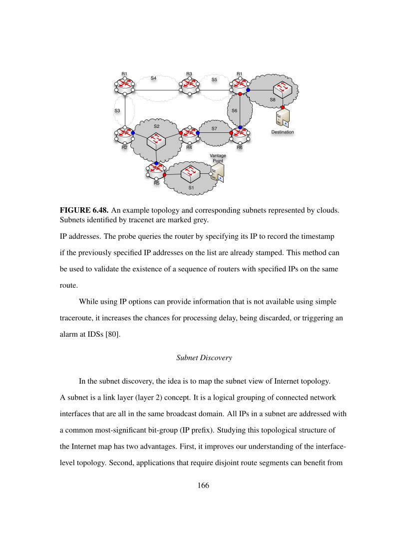
S4R1
S3
S2
S5
S6
S8
S7
S1
R2
R5
R4
R3 R1
R6
Vantage Point
Destination
FIGURE 6.48. An example topology and corresponding subnets represented by clouds.Subnets identified by tracenet are marked grey.
IP addresses. The probe queries the router by specifying its IP to record the timestamp
if the previously specified IP addresses on the list are already stamped. This method can
be used to validate the existence of a sequence of routers with specified IPs on the same
route.
While using IP options can provide information that is not available using simple
traceroute, it increases the chances for processing delay, being discarded, or triggering an
alarm at IDSs [80].
Subnet Discovery
In the subnet discovery, the idea is to map the subnet view of Internet topology.
A subnet is a link layer (layer 2) concept. It is a logical grouping of connected network
interfaces that are all in the same broadcast domain. All IPs in a subnet are addressed with
a common most-significant bit-group (IP prefix). Studying this topological structure of
the Internet map has two advantages. First, it improves our understanding of the interface-
level topology. Second, applications that require disjoint route segments can benefit from
166

this view of the Internet. In the subnet graph, each subnet is a node and subnets adjacent
to one router are connected via an edge. Figure 6.48 shows the topological structure of a
sample network. Corresponding subnets are depicted as clouds.
Subnet level discovery tools such as xnet [256] aim to reveal all ping-able IP
addresses on a subnet. xnet identifies boundaries associated with the IP prefix of a subnet
with a series of tests on IPs that can potentially be in one subnet. The methodology is
developed based on the fact that all IP addresses in one subnet share a prefix and have at
most one-hop distance difference from a vantage point. The problem is that the size of
the subnet is in general unknown. Given IP address t that is n hops away from a vantage
point, xnet probes IPs in the prefix that includes t starting from the smallest /31 prefix
(mate-31). If the probes to all IPs in this prefix travel through the same route and their
hop distances to the vantage point are within the boundaries that support their existence
in the same subnet as t, then the target prefix is expanded and IPs in this expanded prefix
are subjected to the same tests. xnet incrementally expands the prefix until at least one
IP fails the tests. At this point the last successfully tested prefix identifies the subnet that
includes t.
tracenet [255] uses the same principles as xnet to find subnets along a path. It runs
xnet on IP addresses discovered by traceroute from a vantage point to a destination.
Figure 6.48 shows the application of tracenet on a sample topology and identified subnets
are depicted in grey. In this figure, Interfaces discovered by traceroute are marked as
red circles, and blue circles represent interfaces discovered by the xnet component of
the tool. If traceroute returns the incoming interface of each visited router, tracenet is
able to identify the corresponding subnets along the route from the vantage point to the
destination. The principal assumption in tracenet is that routers are configured with an
incoming interface response setting. However, if a router is configured with another
167

setting, xnet discovers an invalid subnet on the path. For instance, in Figure 6.48, if R1
responds with its green interface, S5 is discovered instead of S6 as the fourth subnet on
the route.
Router-Level
The router-level topology shows the routers and the interconnectivity among their
interfaces in the Internet. At this resolution of the Internet topology, nodes represent end-
hosts (with one interface) or routers (typically with multiple interfaces) and links show
layer 3 connectivity between these devices. The topology at this level can be viewed
as the outcome of the aggregation of IP interfaces that belong to a single router. The
following two main techniques are considered for collecting the router-level topology:
– Alias Resolution: Alias resolution [122, 243] or router disambiguation [33]
is a set of techniques used to identify the IP interfaces that belong to the same
router. Such disambiguation is necessitated by the aggregation of traceroute data
that underlies the inference of the router-level topology from the interface-level
topology. The main challenge consists of relating different interfaces of a router
that were discovered in different traceroute measurements.
– Recursive Router Discovery: Another class of techniques employed for obtaining
the router-level topology relies on a router’s capability to be queried for its neighbor
on each interface. The Simple Network Measurement Protocol (SNMP) and the
Internet Group Management Protocol (IGMP) are two methods that can be used to
discover the neighboring routers of a queried router in an intranet and the Internet,
respectively.
168
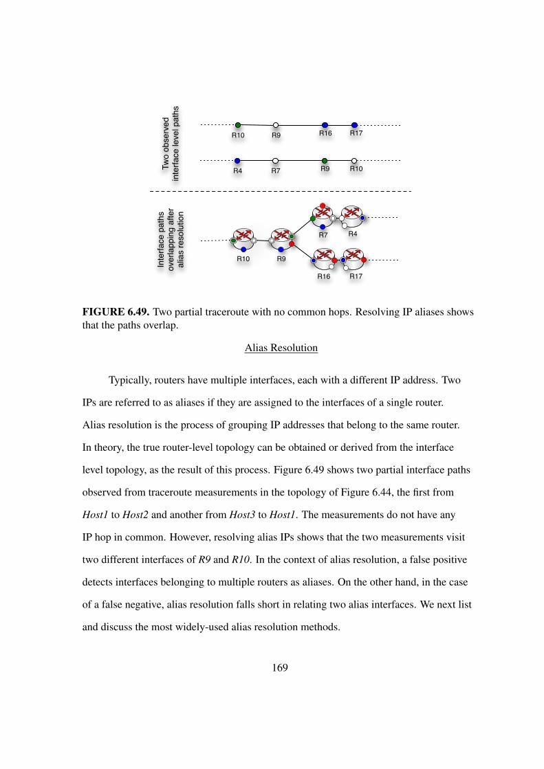
R9R10
R16 R17
R9R10 R16 R17
Inte
rface
pat
hs
over
lapp
ing
afte
r al
ias
reso
lutio
nTw
o ob
serv
ed
inte
rface
leve
l pat
hs
R7R4 R9 R10
R7 R4
FIGURE 6.49. Two partial traceroute with no common hops. Resolving IP aliases showsthat the paths overlap.
Alias Resolution
Typically, routers have multiple interfaces, each with a different IP address. Two
IPs are referred to as aliases if they are assigned to the interfaces of a single router.
Alias resolution is the process of grouping IP addresses that belong to the same router.
In theory, the true router-level topology can be obtained or derived from the interface
level topology, as the result of this process. Figure 6.49 shows two partial interface paths
observed from traceroute measurements in the topology of Figure 6.44, the first from
Host1 to Host2 and another from Host3 to Host1. The measurements do not have any
IP hop in common. However, resolving alias IPs shows that the two measurements visit
two different interfaces of R9 and R10. In the context of alias resolution, a false positive
detects interfaces belonging to multiple routers as aliases. On the other hand, in the case
of a false negative, alias resolution falls short in relating two alias interfaces. We next list
and discuss the most widely-used alias resolution methods.
169

Common Source Address: This technique was proposed and used by Pansiot
et al. [208] in their original traceroute-based topology study and was also implemented
in Meractor [156]. When resolving the alias of the IP address A, Meractor sends a TCP
or a UDP alias probe towards an unused port number of A that replies with an ICMP
“port unreachable” message. This message typically has the IP address of the router’s
shortest-path interface as its source address. If the source IP address of the reply message
is different from A, these two IPs are aliases of the same router. This method is prone to
the router response configuration problems discussed in Section .
Common IP-identification Counter: The packet ID in the IP header is used for
packet reassembly after fragmentation. This technique assumes that a router has a single
IP ID counter. For such a router, consecutive packets generated from the router have
consecutive IP IDs, regardless of the interface from which the packet left the router.
The Ally tool described in [244] and used in the Rocketfuel project implements this
mechanism to detect aliases. It sends a UDP probe packet with a high port number to
two potential alias IPs. The ICMP “Port Unreachable” responses are encapsulated within
separate IP packets and each includes an ID (x and y) in the IP header. Then, it sends
the third packet to the address that responded first. Assuming that z is the ID of the
third response, if x < y < z and z − x is small (e.g. smaller than 200 in case of Ally
[244, 157]), the addresses are assumed to be aliases [244].
Alias resolution based on the ID fingerprint is prone to false negatives due to ID
increment settings on routers that are larger than one [69], the absence of a global IPID
counter for some router [69], or unexpected jitter in the delivery of probe messages. False
positives can also occur as a result of randomly synchronized ID counters of two routers,
but this problem can be mitigated by running more tests after a wait period. The other
major drawback of this ID-based technique is the overhead of running it on a large set of
170
discovered interfaces; its complexity is O(n2) for a set of n interfaces. In the case of Ally,
some heuristics have been proposed to improve the efficiency of the tool by restricting the
possible alias candidates using delays and TTLs [244]. The idea is that alias candidates
should have similar TTLs from different vantage points. Thus, the list of candidate aliases
can be pruned based on the difference in the hop count distance from common vantage
points.
RadarGun [37] mitigates the limitations of Ally by modeling the changes in the
packet ID counter. Instead of directly testing each pair of IP addresses separately, it
iteratively probes the list of IP addresses at least 30 times. Two IPs are inferred to be
aliases if the “velocity” of their corresponding ID counters are consistent in all their
responses. The probe complexity of RadarGun is O(n). The main drawback of this
technique is the potential of error when used on a large list of IPs. Since routers use a
16-bit counter for the packet ID, counter wrap-arounds can occur during the measurement
period. If the probes to the same IP are separated by a period of 40 seconds or longer due
the large number of IPs on the list, multiple wrap-arounds are likely to occur. Although
the designers of RadarGun have accounted for the possibility of a single wrap-around, the
accuracy of the technique diminishes in the presence of multiple wrap-arounds.
DNS-Name: The similarities in DNS names associated with router interfaces can
also be used to infer aliases [244, 243], but this approach also has a number of limitations.
For one, this technique only works when an AS uses a clear naming convention for
assigning DNS names to router interfaces. Second, the complexity of the naming
conventions may require human intervention to resolve aliases which limits the scalability
of this method. Lastly, the technique is known to be highly inaccurate at the AS borders.
The interfaces of border routers usually belong to different ASes which are likely to use
171

Host 1
Host 3
Host 2
R6
R24
R23
R25
R21
FIGURE 6.50. Graph based alias resolution; The green interface succeeds the blue andthe red interface in two traceroute so red & blue would be aliases.
different naming conventions. This observation complicates the use of this technique for
performing alias resolution at the AS borders [122].
Graph-Based Resolution Heuristics: traceroute measurement can offer heuristics
on alias inference [243]. Graph-based alias resolution constructs a directed graph by
overlaying an individual traceroute measurement as illustrated in Figure 6.44. The
“common successor” heuristic suggests which two IP addresses may be aliases. This
heuristic relies on the prevalence of routers that respond to traceroute probes with the
incoming interface. When two traceroute paths merge, the common IP belongs to the
second router on the shared path. IP addresses prior to the common IP should belong to
different interfaces of a single router and hence would be aliases. Figure 6.50 shows a
partial view of a traceroute measurement from Host1 and Host2 toward Host3 in our toy
example. In this example, the black interface succeeds the red interface in one traceroute
and succeeds the blue interface in another traceroute. The heuristic suggests that the blue
and the red interfaces are aliases.
This heuristic falsely infers aliases in the presence of layer 2 switches or multiple-
access clouds. Figure 6.51 depicts an alternate topology to Figure 6.50. The traceroute
172

Host 1
Host 3
Host 2
R6
R24
R23
R25
R21
R26
FIGURE 6.51. False positive in graph based alias resolution due to the presence ofa layer 2 switch; The green interface succeeds the blue and the red interface in twotraceroute so red & blue are inferred to be aliases.
view in both figures are similar, hence the heuristic infers R26’s red interface and R23’s
blue interface are aliases.
The “same traceroute” heuristic identifies IP addresses that can not be aliases. Since
each packet visits a router only once, this heuristic states that two IPs occurring on the
same traceroute can not be aliases.
Analytical Alias Resolution: Given a set of traceroute-derived paths, Analytical
Alias Resolver (AAR) [126] utilizes the common IP address assignment scheme to infer
IP aliases within two opposite paths, one from A to B and the other from B to A. It first
identifies the subnets that are linking the routers (as discussed in ). Then it aligns the two
traceroute paths using the discovered subnets. Alias IPs are easily resolved when point-to-
point links are used and the route is symmetric. To illustrate this technique, consider the
traceroute measurements between Host1 and Host2 shown in Figure 6.52. The top view
shows the two traceroute paths and the identified subnets. The bottom view depicts how
the detected subnets can be used to align the two traceroute paths and resolve aliases.
The Analytic and Probe-based Alias Resolver (APAR) [125] consists of an
analytical and probe-based component. The analytical component uses the same
173

Host 1 Host 2
Host 1 Host 2
2 Tr
acer
oute
s An
d D
etec
ted
Subn
ets
Alia
s R
esol
utio
n U
sing
Det
ecte
d Su
bnet
s
FIGURE 6.52. Analytical Alias Resolution for detecting IP aliases on a symmetric pathsegment.
scheme as ARR, while the probe-based component increases the accuracy of mapping
with limited probing overhead. The probe-based component uses ping-like probes
to determine the distance to each observed IP and mitigates false positives. Any two
interfaces can be aliases only if their hop distance differs by at most one hop from a
single vantage point. This ping-like probe also helps to identify aliases when the source
address of the reply is different from the probed IP (i.e. the Common Source Address
approach).
Record Route Option: The DisCarte tool [235] uses the standard traceroute with
enabled Record Route (RR) IP option to detect IP aliases. For the first nine hops, two
interfaces are captured, one in the forward path and one in the reverse path. Although
the technique sounds intuitive, it is difficult to use effectively in practice because of
inconsistent RR implementations by routers and the complexity of aligning RR data with
traceroute data. DisCarte uses Disjunctive Logic Programming (DLP) to intelligently
merge RR and traceroute data. However, its implementation does not scale to large
datasets. For instance, the application of DisCarte on traces between 379 sources and
376,408 destinations is reported to be so complex that is in fact intractable.
174

Progressive Router Discovery
In some networks, routers store information about their neighboring routers.
Using this information, the topology can be discovered progressively. In a local area
network with SNMP-enabled routers, a list of neighboring interfaces can be identified
from the “ipRoute Table MIB” entry of the router [237]. This technique can be
used recursively to discover new routers and the connectivity between them. Although
accurate, the use of this technique is limited to the interior of an AS and can only be used
by the network administrators with adequate privileges.
More recently, MRINFO has been used to discover the topology at the router-level
using IGMP messages with a similar incremental method [209, 187]. Upon receipt of
an IGMP “ASK NEIGHBORS” message, an IPv4 multicast-capable router replies with
an IGMP “NEIGHBORS REPLY” message that lists all its interfaces and the directly
connected interface of the neighboring router. The applicability of this technique is
however limited to DVMRP multicast-enabled routers, and their number in today’s
Internet is small.
Modeling
The most-cited work on Internet topology modeling is by Faloutsos et al. [102].
In their paper, they relied on the traceroute data collected by Pansiot et al. [208] in mid-
1995 which consisted of the inferred router-level paths taken by packets in the Internet
and produced an observed router topology. One of their main observations was the scale-
free structure of the inferred router topology; that is, the power-law degree distribution of
routers. Intuitively, this finding implies the existence of a small number of high-degree
core routers and a large number of lower degree edge routers. This paper fueled many of
175
the subsequent studies on modeling the Internet’s router-level topology (e.g. [19]) that
aimed at reproducing the observed scale-free structure of the inferred topology.
Although the observations reported in [102] seem plausible, many domain experts
argued that they are indeed erroneous [269]. For one, no publicly available router
topologies exhibit the claimed scale-free structure. For example, in the publicly available
maps of Internet2, there is no evidence of a few highly-connected core routers. Second,
technology constraints and engineering intuition rule out the existence of high-degree
core routers in real-world networks. When configuring a router, network operators are
limited by the tradeoff between traffic volume vs. degree. In particular, a core router
that processes a large volume of traffic on each interface cannot have a large number
of interfaces. On the other hand, routers at the edge of the network carry less traffic
per interface and are capable of having more interfaces. These constraints suggest that
while router topologies can in theory exhibit degree distributions that are consistent
with the reported power-law behavior, the high-degree routers must necessarily be at
the edge of the network and not in its core. Ironically, because of the measurement
platforms used, none of the traceroute campaigns performed in the past would be able
to detect those high-degree nodes at the network edge. Third, there is a clear mismatch
between the observed scale-free topology and the design philosophy of the Internet.
An important requirement of the original DARPA network design was that “Internet
communication must continue despite loss of networks or gateways” [271]. However,
in a scale-free topology, a failed high-degree central router can lead to a partitioning of
the network as shown by Albert et al. [19], an alleged property that became well-known
as the Internet’s “Achilles’ heel”. Lastly, it has been shown that the errors in the router-
level topology considered in [102] are a result of the afore-mentioned limitations of the
alias resolution methods and the fact that the inferred high-degree nodes are an artifact
176

of traceroute’s inability to penetrate opaque layer-2 clouds—the observed topology of
a group of routers at the edge of a layer-2 cloud appears as a mesh-like (e.g. complete
graph) interconnection among all routers and automatically results in the appearance of
high-degree nodes.
Alternatively, Heuristically Optimal Topology (HOT) models have been proposed
to model the Internet topology. These models are based on the method of reverse-
engineering and rely on domain knowledge as an alternative resource as compared to
using data in the form of traceroute measurements to drive the modeling effort. HOT
models are comprised of the following three main components: (i) An objective function
that captures the ISP’s business goals, (ii) technology constraints that dictate that the basic
design of the ISP’s router topology reflect a tradeoff that has to be made between cost and
efficiency, and (iii) the uncertainty in the environment in the form of the traffic demands
imposed on the network. When combining all these ingredients, constraint optimization
can be used to construct an optimal router topology for an ISP with the stated objective
and demands. The construction of such an optimal solution may be NP-hard, but
HOT models are not concerned with optimality. Instead, they are concerned with the
construction of heuristically optimal solutions that result in “good” performance [271]. A
hallmark of the resulting ISP router topologies is the presence of a pronounced backbone
consisting of low-degree but high-capacity routers. Moreover, such a backbone is fed by
tree-like access networks that are built from high-degree but low-capacity routers, with
additional links added for redundancy and resilience.
PoP Level
The PoP-level is the ideal resolution to study the connectivity of an AS when the
objective is identifying all the locations where, at least in theory (i.e. ignoring routing
177

Same AS BackboneTo PoPs of other ASes
To end users
(a) Cookie cutter design used in the PoPof an AS [34, 131]
A3.PoP1
A1.PoP1
A1.PoP2
A1.PoP3 A2.PoP2
A2.PoP1
A3.PoP2
Location 1
Location 2
Location 3
Location
PoP
Legend
(b) The PoP-level topology our example
FIGURE 6.53. PoP level topology.
policies), the AS can exchange traffic with its neighbors. As a result, the topology at this
level is also very useful for potential customers of an AS who may be interested in the
geographic coverage of the AS or in knowing the locations where they can connect.
Terminology & Approaches
The term PoP (Point of Presence) is a loosely defined term within the Internet
community. Internet service providers use PoP to refer to either a physical building with
a specific address where they keep their routers, or a metropolitan area where customers
can reach their services. In the research community, however, a PoP usually means a
collection of tightly connected routers owned by an AS that by design work as a group to
provide connectivity to users or to other PoPs of that same AS or other ASes. Therefore,
PoPs are the reflection of a hierarchical design principle that many ASes apply when
designing their physical infrastructure. Adhering to such a design achieves scalability and
facilitates maintainability of a network.
Network operators often apply “cookie cutter” patterns when designing PoPs
[34, 131]. This modular design strategy simplifies network debugging and management.
178

Figure 6.53(a) depicts an example of such a cookie cutter pattern applied to the design of
a PoP. Certain patterns are explicitly recommended by some network equipment vendors
and show how their products are best used for the buildup of PoPs of certain sizes and
with desirable properties (e.g. redundancy, scalability). The design typically ensures
redundant within-PoP connectivity, access for customers of the AS that owns the PoP,
and connectivity to the rest of the Internet. As a result of this practice, the PoPs of many
different ASes have similar internal (e.g. router-level) structure and are found as repeated
patterns across the global Internet.
A node in the PoP-level topology of the Internet is the PoP of a given AS and is
ideally tagged with the PoP’s owner (i.e. AS) and geographical information (i.e. location).
Inter-PoP links can be categorized into two types. While core or backbone links connect
two PoPs of the same AS, peering links connect PoPs of different ASes. Figure 6.53(b)
shows the PoP-level topology corresponding to the network in Figure 6.44. Each PoP
is identified by its AS and its location. Although AS1.PoP1 and AS3.PoP1 are in the
same location (building), each one is represented by a PoP or node. Backbone links are
represented by lines, and dotted lines show peering links.
Prior studies in this area have considered three different basic approaches for
obtaining the PoP-level topology of the Internet. The first and the most common
approach has been to identify PoPs by aggregating data collected from traceroute
measurements. This method receives either an interface-level or a router- level topology
as input and groups nodes that belong to one PoP. Relevant studies are discussed in
Section .
The second approach is delay-based, but instead of using the per-hop RTT
information from traceroute, it relies on delay estimates obtained from ping
measurements. Yoshida et al. [279] used this technique to detect the PoPs of four major
179
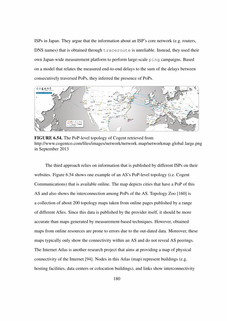
ISPs in Japan. They argue that the information about an ISP’s core network (e.g. routers,
DNS names) that is obtained through traceroute is unreliable. Instead, they used their
own Japan-wide measurement platform to perform large-scale ping campaigns. Based
on a model that relates the measured end-to-end delays to the sum of the delays between
consecutively traversed PoPs, they inferred the presence of PoPs.
FIGURE 6.54. The PoP-level topology of Cogent retrieved fromhttp://www.cogentco.com/files/images/network/network map/networkmap global large.pngin September 2013
The third approach relies on information that is published by different ISPs on their
websites. Figure 6.54 shows one example of an AS’s PoP-level topology (i.e. Cogent
Communications) that is available online. The map depicts cities that have a PoP of this
AS and also shows the interconnection among PoPs of the AS. Topology Zoo [160] is
a collection of about 200 topology maps taken from online pages published by a range
of different ASes. Since this data is published by the provider itself, it should be more
accurate than maps generated by measurement-based techniques. However, obtained
maps from online resources are prone to errors due to the out-dated data. Moreover, these
maps typically only show the connectivity within an AS and do not reveal AS peerings.
The Internet Atlas is another research project that aims at providing a map of physical
connectivity of the Internet [94]. Nodes in this Atlas (map) represent buildings (e.g.
hosting facilities, data centers or colocation buildings), and links show interconnectivity
180

between them. Atlas is built using resources such as online maps and other publicly
available information from different repositories or databases.
Aggregation Methods
In the following, we discuss prior studies that focused on interface and router
aggregation to unravel PoP-level topology. Due to the importance of geography at this
resolution, we also discuss the studies that examined geographical characterization of
PoPs.
The first study that focused on the discovery of PoPs was Rocketfuel [244]. It tried
to infer the structure of an AS using traceroute measurement and used the PoP-
level topology to visualize an AS infrastructure. Rocketfuel first identified alias IPs using
Ally’s packet ID counter method. It then leveraged the inferred DNS naming conventions
used by an AS to geolocate the discovered IPs using a tool called UNDNS. UNDNS uses
a large set of regular expressions to extract city and airport codes embedded in DNS
names and infer the geographical location of an interface. In the end, Rocketfuel groups
interfaces that are mapped to one and the same geographical location into a PoP.
iPlane [177] extends the approach advanced by Rocketfuel. First, a Meractor-like
[156] alias resolution is used to identify routers. Additionally, iPlane uses a mate-30
heuristic similar to AAR [126] and identifies subnets to find candidate alias pairs. A
Packet ID fingerprinting technique is used on the candidate alias pairs to infer aliases
[244]. Next, DNS names are used to geo-locate routers and group them into PoPs.
However, this step is riddled with issues. For one, for some routers, there is no DNS name
assigned to any of their interfaces. Also, there is no guarantee that assigned DNS names
contain any relevant geography-related information. Furthermore, DNS misnaming can
introduce error to this mapping process. DNS names are voluntarily assigned by network
181

administrators and interface misnaming is fairly common especially due to relocating
routers and using old assigned DNS names [281]. In a final step, iPlane considers all
routers that it has not been able to map to a location and assigns them a location using
a clustering approach that is based on a notion of similarity between interfaces with
respect to routing and performance. To this end, iPlane probes all interfaces with ICMP
echo probes from different Planet Lab nodes. Each interface is assigned a vector in
which the ith element is the length of the path from the ith vantage point. Hence the PoP
detection problem is translated into a clustering problem involving these measurements,
and interfaces in one cluster are assumed to belong to the same PoP.
Note that both projects rely heavily on the capability to extract information
about the location of a router from the DNS name assigned to it. The structure of DNS
names was recently revisited by Chabarek et al. [62]. Their study shows that aside from
geographical information, DNS names may include information about interface types,
bandwidth, and router manufacturers. However, meaningful encodings are more common
in the core of the Internet [62], and the naming structure tends to be strongly tied to the
AS that owns the router [105].
Another popular approach is to use geo-IP databases to assign a location to an IP
address. Tian et al. [252] use these databases in conjunction with a heuristic approach
to locate router interfaces. They initially rely on existing geo-IP databases to annotate
the given interface level topology graph with geographic information. The resulting
annotated graph contains some clusters corresponding to each city. Their heuristic
technique re-annotates an interface to a new location if the new annotation results in more
coherent groupings, where more links are inside a group. Each group is detected as a
PoP. One basic problem with this approach is the well-known inaccuracy of the freely or
commercially available geo-IP databases [212, 239, 124].
182

A PoP consists of a set of routers with high interconnectivity among them. Links
inside a PoP are usually very short, implying small delays in general. These properties
were used by Feldman et al. [104, 233] to propose a more automatic approach for
detecting PoPs. In their graph-based approach, network “motifs” are used to detect
repeated patterns in traceroute-derived interface-level topologies collected by
DIMES [231]. These repeated patterns are used to identify tightly connected interfaces.
To this end, they ignore all links with a delay above a certain threshold (5 ms); these links
are likely to be long-haul connections between distant PoPs. This step generates a graph
with disconnected components, each of which is a candidate to represent either a single
PoP or multiple PoPs. Different refinement techniques are applied to either split one
component or merge different components to detect the PoPs based on graph motifs. To
geolocate the inferred PoPs, they use several geolocation services including the MaxMind
GeoIP [185]. Finally, they validate their PoP-level topology using a DNS name-based
geo-localization data base and two geo-IP data bases. Their claim is that by not using the
DNS names as part of their methodology, this information can be used as “ground truth”
to validate the accuracy of their technique. Unfortunately, the accuracy of using DNS
names to infer geographical location of an interface is questionable [281].
AS-Level
The Internet’s topology at the AS-level is typically modeled using a simple
graph where a node is an AS identified by an AS number. As previously described, an
Autonomous System or AS is commonly defined as a collection of IP prefixes under
the control of a single network operator that presents a common, clearly defined routing
policy to the Internet [132]. In such an AS graph, links represent logical connectivity
between two ASes and are labeled according to the type of connection; customer-
183

provider, peer-peer, and sibling relationship. The logical connectivity between two ASes
usually represents multiple physical connections that are established between PoPs of the
two ASes, presumably to enable the efficient exchange of traffic between them.
This graph representation of the AS topology has a number of limitations. First,
each AS has a geographical footprint that may overlap with the footprint of another AS.
This feature cannot be illustrated using a simple node to represent an AS, unless the
node is replaced by a region that covers the area in question. Second, ASes are widely
considered to be coherent entities with a clearly defined routing policy. However, for
historical reasons or due to their often global reach, some ASes use different policies
in different parts of their network. In this context, Muhlbauer et al. [196] demonstrated
that treating ASes as atomic structures is a severe over-simplification and negatively
impacts our understanding of inter-domain routing. Third, the fact that many inter-AS
links represent multiple geographically dispersed physical AS connections cannot be
captured by a simple graph. Fourth, IXPs also complicate the AS-level topology by
providing connectivity between many ASes, most commonly through layer 2 multiple
access clouds. As a result, in a realistic AS topology graph, IXPs should be modeled as
links that connect more than two ASes. Together, these issues suggest that a hyper-graph
[223] provides a more detailed and informative structure of the Internet’s AS topology.
However, these numerous limitations notwithstanding, simple graph representations of
the AS-level topology are considered to be useful and have been studied for the past two
decades to a great extent.
AS Topology Data Sources
Techniques for discovering the AS-level topology rely mainly on the following
three data sources: BGP information, traceroute measurements, and Internet Routing
184

Registries (IRR) [139]. Below we discuss each type of data source and its limitations in
more detail.
BGP Information: BGP is the de-facto standard inter-domain routing protocol of
the Internet. BGP is a path vector protocol in which routing decisions are made based
on reachability via the advertised AS paths and expressed network policies. The term
“reachability protocol” has been used to emphasize this characteristic of BGP. BGP uses
the AS number to specify the origin AS of a prefix and ASes along the path to reach the
origin AS.
BGP data has been collected by various projects and has subsequently been used
in different forms. BGP information can be obtained from various resources, including
(i) BGP archive: Oregon RouteViews [12] and Reseaux IP Europeens (RIPE) Routing
Information Service (RIS) [9] collect BGP route information through a set of route
collectors also known as BGP monitors or vantage points. The original purpose of these
projects was to help network operators with troubleshooting and debugging tasks, and
for these purposes, the data has proved to be invaluable. Both services collect routing
table dumps and route update traces on an ongoing basis. While BGP dumps show the
best path to reach other ASes, the back-up links and the dynamic nature of BGP routes
are more likely captured by “route updates”. (ii) Route Servers: A route server is a BGP-
speaking router that offers interactive login access via telnet or ssh and permits third
parties to run many non-privileged router commands [280]. For example, BGP summary
information can be obtained by executing the “show BGP summary” command. (iii)
Looking Glasses: A looking glass is a web interface to a BGP router which often allows
basic BGP data querying and supports limited use of debugging tools such as ping and
traceroute [280].
185

BGP information was the first data source used to map the AS-level topology [121].
Two representative studies that use both BGP dumps and updates to capture the AS-level
topology are [280, 179]. Although passive collections of BGP tables and updates have
fueled many studies concerned with the AS-level topology, there also have been efforts
that used active measurements of BGP. In this context, a BGP beacon [180, 49] is a router
that actively advertises and withdraws prefixes. Observing the resulting announcements
from the perspective of different route collectors within the larger Internet enables
researchers to infer some of BGP’s overall behavior (e.g. protocol convergence time
and the average AS distance an advertisement travels in the control plane). In a similar
manner, BGP route poisoning prevents BGP announcements from reaching an AS. Bush
et al. [49] used this technique to measure the prevalence of default routes in the Internet
and explain the differences in the AS-level topologies obtained from control vs. data
plane measurements.
Using BGP for inferring the AS-level topology has several advantages. First,
compared to Internet registries, the data collected from BGP shows the actual reachability
as seen from the perspective of the Internet control plane. Hence, the data is typically not
prone to being stale, obsolete or incorrect. Second, BGP updates can be used to study the
dynamic behavior of Internet routing which, in turn, can reveal otherwise hard-to-detect
backup links. Third, engineering solutions such as the use of BGP beacons and route
poisoning can be applied on top of BGP to improve our view of the topology.
Despite all its advantages, using BGP information to infer the AS-level topology
is not without limitations. The main reason is that BGP is merely an information hiding
protocol and only indicates reachability, not connectivity. More specifically, AS path
announcements are primarily used for loop detection. For traffic engineering reasons,
adding an AS in the announcements is not uncommon. Also, ASes may announce AS
186

paths that do not correspond to real paths [196]. Moreover, as a path vector protocol, BGP
does not announce information about every available path. As a result, back-up paths
might never appear in the BGP dumps. In fact, since BGP only announces the best paths,
many alternative AS paths remain hidden from any route collector. Since route collectors
are normally deployed in larger ISPs and mostly in the US and Europe, their observed
AS-level topology is biased to be more complete for these regions. Additionally, even if
the route collectors were randomly placed in different ASes, the likelihood of discovery
of an AS relationship is proportional to the number of ASes using that link [133, 49]. This
finding proves a measurement bias in BGP-based AS topologies because P2P links are
only used for traffic originating from the customers of any of the peering ASes. Hence
P2P AS relations are in general much harder to discover than C2P AS relationships [133].
In fact, the majority of the missing AS links in AS-level topologies inferred from BGP
data are known to be P2P links [202]. The severeness of this bias and the resulting
degree of incompleteness of even the most-carefully inferred currently available AS-level
topologies have recently come to light with the discovery of massive amounts of public
peering links (i.e. P2P AS connections) at a large European IXP [13], most of which have
remained invisible in presently available BGP data.
traceroute Measurement: Another approach to discover the Internet’s
AS-level topology is to use the interface-level topology obtained from traceroute
measurements. In this approach, each IP in a traceroute is mapped to its corresponding
AS. BGP routing tables and IRR can be used to map an IP to an AS based on the IP
prefixes that are announced by the AS [182]. Consecutive IPs that belong to two different
ASes reveal the connectivity between ASes.
This technique has the advantage of revealing a potentially more detailed view
of the AS-level topology. Recall that ASes can be connected at multiple locations.
187

traceroute-based measurements allow us to distinguish between multiple inter-AS
connections between two ASes. In addition, traceroute measurements often use more
vantage points, mainly because deploying a traceroute vantage point is much easier than
deploying a BGP route collector. As a result, the AS-level topologies inferred from data
collected by large-scale traceroute measurement campaigns are generally considered to be
more complete than those collected from BGP information [231, 68, 224].
Apart from the limitations of traceroute that we discussed in Section , active
measurements in the data plane have other limitations when used for mapping the AS-
level topology. First, IP-to-AS mapping is a non-trivial task. Prefix registries are often
incomplete and using BGP for mapping IPs to AS numbers is not accurate due to BGP’s
information hiding characteristics. Second, discovering a false inter-AS connection is
likely due to inconsistencies in router responses [68, 282]. Third, private IPs and IPs in
the carrier-grade NAT (large-scale NAT) IP range may also appear in a traceroute which
renders the IP-to-AS mapping impossible for these IPs[282].
Finally, it is worth mentioning that when measuring the AS-level topology using
BGP and traceroute measurements respectively, what is really measured are the Internet
control and data planes. While the control plane focuses on “reachability”, the data plane
is all about “connectivity”. The inconsistencies in the data plane and the control plane
measurement may result in different and inconsistent views of the Internet AS-level
topology. In general, these issues stem from the limitations of the data that is used to
infer the topology and the lack of knowledge about the effects of these limitations on the
observed topology [49]. For instance, “default routing” limits the view of passive BGP
measurements while it has the potential of enhancing the view of active measurements
(e.g. observe the route). The general consensus is that the AS-level topology inferred
from measurements in the data plane results in a more accurate and complete view as
188

compared to relying on measurements in the control plane [49, 271, 223]. However, [13]
is a reminder of the caveat associated with this consensus.
Internet Routing Registries: The Routing Arbiter Database (RADb) provided by
IRR is a group of look-up databases maintained by several organizations. These databases
are designed to provide fundamental information about routing in the Internet, including
documented routing policies, regulations, and peering information
The main advantage of using IRR is its simplicity. All the information is accessible
via the WHOIS command and can be obtained through FTP servers. Being based on
data provided by the different ASes themselves, this resource does not exhibit the sort
of limitations that data obtained through measurements have. However, when using
this resource, extra care is needed for different reasons. For one, since these registries
are populated and maintained on a completely voluntary basis, the available data may
be stale or incomplete due to confidentiality reasons, personnel changes in the different
ASes, or because of the overhead of updating an external data store. For instance, reports
that checked the accuracy of RIPE-provided data show inconsistencies in different IRR-
provided databases [219].
AS Relationship & AS Tiers
Although the logical AS-level topology is interesting in itself, to be more useful in
practice, the inter-AS routing policies should also be inferred. We recall that the business
relations between connected ASes are broadly classified into [137] (1) Customer-Provider
(C2P), (2) Peer-Peer (P2P), and (3) Sibling relations. From a financial perspective, in a
189
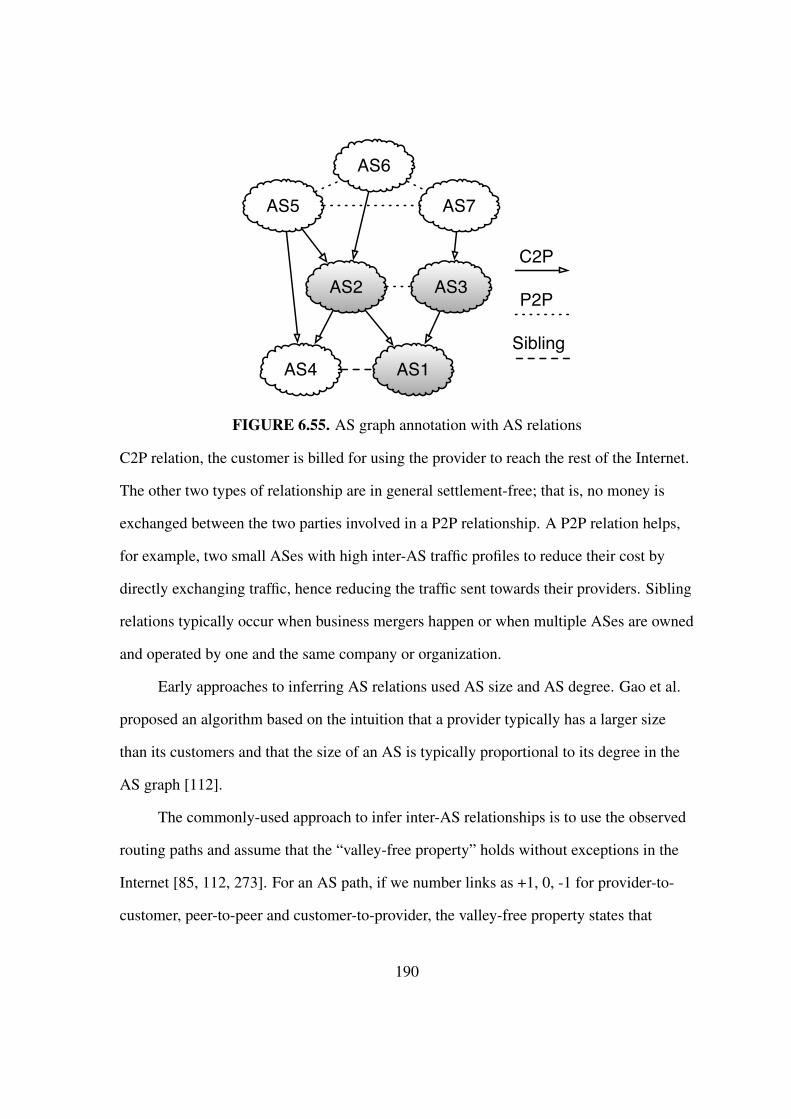
AS1
AS3AS2
AS4
AS7
AS6
AS5
C2P
P2P
Sibling
FIGURE 6.55. AS graph annotation with AS relations
C2P relation, the customer is billed for using the provider to reach the rest of the Internet.
The other two types of relationship are in general settlement-free; that is, no money is
exchanged between the two parties involved in a P2P relationship. A P2P relation helps,
for example, two small ASes with high inter-AS traffic profiles to reduce their cost by
directly exchanging traffic, hence reducing the traffic sent towards their providers. Sibling
relations typically occur when business mergers happen or when multiple ASes are owned
and operated by one and the same company or organization.
Early approaches to inferring AS relations used AS size and AS degree. Gao et al.
proposed an algorithm based on the intuition that a provider typically has a larger size
than its customers and that the size of an AS is typically proportional to its degree in the
AS graph [112].
The commonly-used approach to infer inter-AS relationships is to use the observed
routing paths and assume that the “valley-free property” holds without exceptions in the
Internet [85, 112, 273]. For an AS path, if we number links as +1, 0, -1 for provider-to-
customer, peer-to-peer and customer-to-provider, the valley-free property states that
190

any valid path should only see a sequence of +1’s, followed by at most one 0, followed
by a sequence of -1’s. The type of relationship assignment can be formulated as an
optimization problem. Given an undirected graph representation of the AS topology and
a set of AS-level paths, the aim is to assign policy labels to the links in such a way as to
minimize the number of invalid routes. Although this problem is proven to be NP-hard,
some approximation techniques have been presented in the literature [85].
An alternative approach is to check the consistency of inferred relations (using
any of the above methods) with other measurements [181]. For instance, Muhlbauer
et al. [196] used traceroute measurements to estimate the accuracy of the inference by
comparing the inferred routes and the real routes. In their approach, they use multiple
quasi-routers to capture route diversity within the ASes.
Traditionally, the AS-level topology is widely regarded to be hierarchical in nature,
where ASes are categorized into different tiers [85, 273]. Tier-1 ASes are defined as those
that don’t buy transit from any other AS. These tier-1 ASes form a complete graph (i.e.
full mesh connectivity) at the highest tier. Tier-2 providers are customers of the tier-1
ASes using them for Internet transit. Additionally, tier-2 ASes use peer-peer relations
with other tier-2 ASes to decrease the transit cost. This hierarchical structure can be
extended to more levels. However, this perception is changing. First, many new ASes
(e.g. content providers and Content Distribution Networks (CDN)) are inherently different
from the traditional ISPs and also tend to have many connections at various locations.
These new types of ASes do not fit within the traditional tiered AS hierarchy. In addition,
new studies explain this changing perception using the abundance of missing links and
the limited observability of P2P connections in currently studied AS topologies [271].
Although the existence of large transit ASes at the highest tier remains valid, the tier-
based hierarchical view is replaced by a flatter but more modular view. Figure 6.55 shows
191

an example of an annotated AS graph. AS1, AS2, and AS3 are the ASes in our previous
examples. AS5, AS6, and AS7 are tier-1 ASes forming a full mesh at the highest tier.
However, there is no longer a pronounced hierarchical structure below these tier-1s.
Coverage & Completeness
As of 2011, diligently-inferred AS-level topologies consists of approximately
40,000 ASes and 115,000 to 135,000 edges, with 80,000-90,000 C2P links and the rest
P2P links [271]. While such topologies seem to be complete with respect to their node
sets (i.e. ASes), their edge sets are typically inaccurate and miss a large number of AS-
links, especially with respect to P2P links.
A great deal of research has been dedicated to studying the question of
completeness of inferred AS-level topologies. The “Lord of the Links” study [133]
compares BGP routing tables, Internet Routing Registries, and traceroute measurements,
cross validates the topology captured from these various sources and captures a more
complete view of the AS topology. The authors of this study also extract a significant
amount of new information from the operational IXPs worldwide and use this information
in their cross validation process.
The incompleteness of the Internet AS map has also been studied (e.g. [202, 203]).
Oliveira et al. [204] use ground truth data provided by a large tier-1 ISP to validate the
accuracy of their derived AS maps for a few target ASes. The ground truth is built upon
router configuration files, syslogs, BGP command outputs, and personal communications
with the network operators. Oliveira et al. [202] categorize the missing links into hidden
and invisible links. Invisible links are missing due to the limitations imposed by the
placement of vantage points. Hidden links, on the other hand, can be found with further
measurements. On the active measurement side, the importance of the distribution of
192

traceroute vantage points is studied by Shavitt et al. [232]. Given a large set of vantage
points, they use sensitivity analysis and measure the changes in the discovered topology
using a different number of vantage points. They show that although increasing the
number of vantage points can help reducing sampling bias, it can not overcome the bias
due to their placement. They conclude that measuring from within a network is important
for discovering more of its links, mainly for low-tier ASes.
More recently, the AS-level map underwent a major revamping due to the
availability of ground truth data from one of the largest IXPs in Europe with some 400 AS
members [13]. The main finding was that in this single IXP, there are more than 50,000
P2P links visible, which is more than the total number of P2P inferred Internet-wide.
This finding suggests the total number of P2P links in the Internet is likely to be larger
than 200,000. More importantly, this recent observation shows that the presently-used
AS-level Internet topologies are far from complete, with much room for improvement.
Geolocation
Apart from prior studies on the geographic locations of PoPs of an AS, little has
been done on mapping the geography of ASes (i.e. the geographical area that is served by
an AS). The notion of the geography of an AS has become even more delicate with the
emergence of newer types of ASes such as larger content providers, CDNs and and cloud
providers. While the geography of a traditional AS like 7018 (AT&T North America)
is well defined in the sense that it covers the US, defining the geography for ASes like
15169 (Google) or 20940 (Akamai) is more complicated as they cover roughly the whole
globe.
Internet registries and directories such as PeeringBD [211] provide a plethora of
information about the geography of ASes. PeeringDB for instance provides a list of
193

public and private facilities where an AS has PoPs. Similar to other online resources,
these directories are easy to use but can be out of date and incomplete.
The geographical footprint of eyeball ASes (ISP that serve residential costumers)
was studied in [214]. Using large-scale measurements from Peer-to-Peer applications, the
authors of this study identify a large set of end-host IPs. These IPs are then mapped to
ASes. Next, the geographical coverage an of AS is estimated using the geo-density of a
large number of its customers. Different IP-to-geolocation databases are used to find the
location of an IP address, taking into account the errors inherent in those databases. Since
a large volume of customers are used to map the geo-footprint of an AS, the potential
error in IP-to-geo mapping does not influence the final discovered coverage of the AS.
Modeling
Several studies have examined the presumed AS topology of the Internet from a
graph-theoretic perspective and have proposed different graph-based network models.
However, there is no consensus on which of the studied models is more relevant or
realistic due to the incompleteness of the inferred topologies. Zhou et al. [285] propose
a growth model with Positive-Feedback-Preference which reproduces many topological
properties of inferred AS-level topologies. Their model, however, uses the Skitter [54]
traceroute dataset to infer the target AS-level topology. As discussed earlier, this dataset
suffers from well-known limitations of traceroute-based mapping efforts. For instance,
the observed power-law degree distribution of this AS topology is known to be due to
the bias in the measurement techniques [223, 271]. Mahadevan et al. [179] used the AS
topologies inferred from multiple data sources that included BGP, traceroute and WHOIS
measurements. They compared the resulting graphs from a graph-analysis perspective and
reported that the “joint degree distribution” can be used to characterize the Internet AS
194

graph. They also showed how the data collection peculiarities can explain differences in
their graph comparison study.
The evolution of the Internet AS map has also been investigated. The main
challenge with respect to the long-term evolution of the topology is to distinguish
between topology changes and changes due to routing dynamics. Oliveira et al. [205]
compose a model that distinguishes between the two different events. Their findings
suggest that the impact of transient routing dynamics on topology decreases exponentially
over time. Dhamdhere et al. [82, 10] take a different approach in characterizing the AS
map evolution. They compare the AS maps collected during the past 12 years using BGP
dumps. They report that the AS-level topology was growing exponentially until 2001,
but this growth has settled into a slower exponential growth in terms of both ASes and
inter-AS links. However, the average path length has remained the same. These measured
graph properties can be used in topology generators to build AS-level models of the
Internet.
In view of the latest understanding of the quality of the different inferred AS-
level topologies that have been studied in the past, a recent common theme in AS
topology modeling has been that a proposed model is only as good as the underlying data.
Moreover, there has been increasing awareness that any strict graph-theoretic treatment of
the AS-level Internet topology necessarily misses out on the key fact that this topology is
a construct that is mainly driven by economic factors and decisions. [64, 65, 82] are early
attempts at addressing these points. For example, Chang et al. [65] use a policy-based
graph model, where policies are implemented in a simulated environment and effect how
ASes decide to create new AS relations. Similar to the HOT modeling approach for the
router-level topology, their model follows the reverse-engineering approach. As part of an
AS’s decision making process, they consider the gain from P2P links and C2P links, using
195

simulated traffic demands. Using different profiles for ASes with different objectives,
they model the behavior of these ASes and model the Internet using an evolutionary
framework. To validate the model, they use publicly available measurements and perform
their own measurement experiments to check for consistency of the model with the
real-world Internet. Lodhi et al. [172] build on this initial attempt described in [64] and
consider an agent-based network formation model for the AS-level Internet. The proposed
model, called GENESIS, is based on realistic provider and peering strategies, with ASes
acting in a myopic and decentralized manner to optimize a cost-related fitness function.
Discussion
Examples of “Big (Internet) Data”
The Internet is arguably the largest man-made complex system. As such, it has
attracted the attention of the larger scientific community, and the number of studies
on topics related to measuring, analyzing, modeling, predicting and providing a basic
understanding of the structure and behavior of this highly-engineered network has
increased dramatically over the last two decades. Importantly, this increase in Internet-
related publications started with the initial availability of large new datasets of Internet-
specific measurements (e.g. traffic traces [167, 210], routing data [12, 121]), and the
subsequent explosive growth has been largely driven by “big Internet data”; that is,
publicly available or proprietary datasets resulting from large-scale measurement
experiments that tend to produce voluminous amounts of observations.1 Typically, these
observations have rich semantic content and often provide useful information about the
1As part of the Ark project [51] alone, some 10 billion traceroute measurements have beencollected during September 2007 and January 2011.
196

Internet as a whole or about its individual components (e.g. ASes, routers, protocols,
services).
In general, the producers and owners of the various types of “big Internet data” are
network researchers or operators, and while their reasoning for collecting data may vary,
practical reasons (e.g. for trouble shooting) almost always trump altruistic arguments
(e.g. for the good of science). For example, in the case of Internet topology-related big
data which is the focus of this survey, the realization that the influence of the Internet’s
structure or topology on the network’s functionality (and vice versa) is in general not
well-understood but is the root cause of many encountered networking problems has
been the main motivation for data collection projects such as Route Views [12] and RIPE
RIS [9]. The measurements from these and similar efforts have proven to be invaluable
for purposes such as network management, trouble-shooting, and debugging. In addition,
they have also informed the design of new protocols, applications, and services and have
contributed to an increased awareness of the vulnerability of the Internet to a growing
number of ever more potent cyber threats.
Economics of the Internet and Interconnection
Economics is the driving force for two networks or autonomous systems (ASes)
to interconnect or peer with one another for the purpose of exchanging traffic between
them directly rather than indirectly (e.g. by relying on a third party such as a transit
provider). In case the two parties determine that interconnecting makes sense financially,
they then must decide on the geographic locations where their networks will physically
interconnect as well as on the type of interconnection. For example, the two parties are
likely to first examine opportunities where both networks already have a presence in the
same city or even in the same colocation facility in a city and then consider the available
197

interconnection options. Among the available peering options, the most common ones are
private peering and public peerings. Two networks peer privately by buying a dedicated
fiber or point-to-point circuit (also called cross-connect, or x-connect, for short) from the
colocation facility provider where they are both customers (e.g., rent cabinet space for
accommodating their routers and servers). That same facility may also house (parts of)
the switching fabric of an Internet eXchange Point (IXP), in which case the two networks
have the opportunity to establish a public peering by simply purchasing and utilizing a
port at the IXP2.
For the past 15+ years, researchers have studied in great detail the non-physical
construct known as the Internet’s AS-level topology, where nodes are (routed) ASes and
links are logical entities indicating that the involved ASes interconnect with one another
in one or more locations around the world (e.g. see [10, 223, 271] and references therein).
However, these past efforts have largely ignored the physical realizations of these logical
AS-links; that is, the different geographic locations (e.g. city, colocation facility) where
two networks interconnect physically to directly exchange traffic with one another.
To appreciate the need for a better understanding of physical interconnections in the
Internet, consider the case of the U.S. where there is a range of small to large colocation
companies that are in the business of selling interconnections. As for-profit companies
that are often also publicly traded, they are mandated to provide business-specific details
in their SEC filings, and a cursory reading of the financial statements released by these
for-profit companies shows that Equinix dominates the x-connect market in the US with
some 97K connections (as of 1Q 2016) [3], followed by companies such as Telx3 with
some 50K and CoreSite with about 20K [106, 152, 7, 77, 76]. In terms of the underlying
2Recent technological advances, especially the introduction of VLAN services over an IXP switchingfabric, have started to blur the notions of public and private peering.
3Telx was acquired by Digital Realty Trust in late 2015.
198

economics, with an approximate monthly cost of $300 for a x-connect in some of the
major cities in the US [251], in the case of Equinix, the revenues from selling x-connects
in the US alone amount to about $270M per year [99, 100]; sale of x-connects is the
second largest revenue generator for these companies after selling cabinet or colocation
space in their buildings. However, little to nothing is known publicly about where all
these x-connects in the US or elsewhere are located (i.e. in which colocation facility
in which city) and which ASes are parties to which x-connect. As a result, developing
a principled approach to accurately answering questions such as “In which cities and
with which networks a major content provider (e.g. Google or Netflix) establish private
peering? , and with whom?” or “Where are all the x-connects that Netflix uses to deliver
its content to an eyeball provider like Comcast and which networks are parties of these
interconnections?” has loomed as an important open problem that has vexed network
researchers and operators alike. Such an approach would not only allow for a systematic
assessment of reported peering disputes (e.g. see [175] and references therein), but would
also complement recent work on mapping the US long-haul fiber-optic infrastructure [96]
by adding the missing x-connects between service providers in colocation facilities across
the US. In turn, such an augmented map of the US long-haul fiber-optic cables could be
used to aid recent efforts for a speed-of-light Internet [238] by examining the nature of
the delay that is due to packets traversing x-connects (i.e. being handed over from one
network to another) in different colocations along their end-to-end paths.
The current lack of transparency about the geography of (and parties to) x-connects
is akin to an earlier problem that concerned public peerings at IXPs and arose from a
need to understand which member ASes of an IXP peer publicly with one another; that
is, exchange traffic over the IXP’s public switching fabric. However, the task of mapping
the x-connects inside a commercial colocation facility is inherently more difficult than
199

mapping the public peerings between the different members of an IXP. At IXPs, member
ASes use their IXP-assigned addresses to establish peerings with other member ASes.
The existence of an IXP-assigned address within general-purpose traceroute probes is a
commonly used heuristic for inferring the presence of a public peering link between two
member ASes of an IXP [274, 24, 224, 116, 13]. In the absence of any such comparable
solid “hints” or indicators, the problem of inferring the presence of x-connects between
ASes that are customers of one and the same colocation facility is extremely challenging
and requires creative new solutions.
Lessons Learned & a Check List
A key lesson learned from surveying the existing literature on Internet topology
discovery has been the realization that “more is not always better.” That is, using more
measurements from the same traceroute campaign or from the same set of BGP
monitors is now viewed as a non-starter for solving the severe degree of incompleteness
of all past and current inferred Internet topology maps at all four levels. In this sense, “big
Internet data” is a reminder that the extraction of key information from big data cannot
rely on big data analytics alone but is often intimately tied to applying detailed domain
knowledge and hard-to-quantify engineering intuition.
A closely-related lesson is that in the context of data sources for Internet topology
discovery, “less can actually be more” in the sense that a strategically-placed vantage
point can have much better visibility in certain substrates of the Internet topology than a
large number of vantage points that have been selected in an ad-hoc fashion or are tied to
a fixed measurement platform. The recent IXP studies [13, 67, 66] are prime examples
that highlight this point.
200

At a more technical level, the main lesson from getting to know the lay of the
land with respect to Internet topology discovery is that “details matter.” For example,
using traceroute measurements “blindly” without knowing the technique’s main
idiosyncrasies detailed in Sections 6.3 and 6.4 is bound to lead to incorrect result, flawed
claims or wrong findings about the Internet in general and its topologies at the different
levels in particular. Similar comments apply to the “blind” use of BGP measurements or
other data sources that have been tapped for Internet topology discovery.
Even though many of the datasets that have been used in the context of Internet
topology discovery have been created by network researchers, as owners of these
datasets, they have largely failed to communicate to the users or consumers of their data
the main limitations and issues. A notable exception is the original work by Pansiot
and Grad [208], but unfortunately, their diligent efforts listing critical issues with
traceroute and highlighting important artifacts in the obtained data has been all but
ignored and forgotten by the networking community [161]. As illustrated in this survey,
this failure to properly educate the networking community and scientific community
at large about the pitfalls and drawbacks of using the available data “as is” has led to
numerous dead-end research efforts. Importantly, it has in general hampered progress in
this important area of Internet research as evidenced by a lack of high-quality maps of the
Internet topology at any of the described levels, even to this date.
To improve upon this unfortunate situation, we provide in the following a checklist
that is a compilation of the main lessons learned from past work in this area. We
encourage every researcher interested in working on Internet topology-related problems to
consult this checklist before embarking on their own work of any measurement, analysis
or modeling efforts that make use of tools, datasets, or methods that have been precisely
201

addressed in past work in this area. Our checklist consists of a number of increasingly
more detailed questions for that any interested researcher should ask upfront:
– What datasets are used or generated for the planned work?
– What techniques have been used to obtain the data?
– What are the (known) limitations of the used techniques and what is known about
how these limitations impact the quality of the data?
– How can the known data quality issues impact the results of the planned work?
– If the known data quality issues are claimed to be minor, do the obtained results and
findings withstand further scrutiny based on alternative data or available domain
knowledge?
In a nutshell, by raising researchers awareness of the limitations of the used
measurement techniques and how they may affect the resulting data, researchers will
be able to answer for themselves whether or not the used tools, datasets, or methods are of
sufficient quality to successfully tackle the particular research problem they are interested
in. We view consulting this straightforward checklist as a first step that will hopefully
prevent researchers from repeating some of the same or similar mistakes that have been
made in the past and that have negatively impacted the progress in this important area of
networking research.
Outlook
If past experience is any indication, progress in terms of discovering more accurate,
complete, and internally consistent Internet topologies at different levels will come
from renewed effort that gives quality priority over quantity when it comes to Internet202

measurements. Here, quality refers first and foremost to the choice of the locations of
the vantage points used in large-scale measurement campaigns but also includes the
diligence necessary to eliminate as many of the known idiosyncrasies inherent in most
of the presently-used measurement techniques. Recent examples that demonstrate the
promising results that measurement platforms with purposefully-chosen vantage points
can produce over conventional measurement infrastructures in the context of Internet
topology discovery are seen in [24, 13, 224, 116]. However, these are early efforts, and
the potential for carefully and purposefully-designed next-generation measurement
platforms with programmable vantage points in strategic locations indicates an exciting
future for research in Internet topology discovery.
Regarding many of the measurement techniques underlying Internet topology
discovery, we have shown in this survey that despite gradual and significant progress
and achievements in increasing our understanding of the many idiosyncrasies of
traceroute or BGP and how they affect the integrity and quality of the resulting
data, the Internet topologies that one can infer are at best inadequate. A main reason for
this unfortunate situation is that neither traceroute nor BGP have been designed for
Internet topology discovery but have been “re-purposed” by researchers for that very task.
Instead of accepting this situation as a “fait accompli”, the time seems ripe to try and do
away with the utilization of such “engineering hacks” for the purpose of Internet topology
mapping. To this end, we advocate for the pursuit of a “clean slate” design of techniques
and/or protocols for the explicit and exclusive purpose of Internet topology discovery
at a given level. The objective of such an effort is plain and simple: the design of new
measurement techniques that enable researchers to measure what they want to measure,
and not just what they can measure.
203

Lastly, main Internet topology-related modeling studies covered in this survey
indicate a clear preference for treating Internet topologies at any level strictly as graph-
theoretic constructs and relying mainly graph theory to study their properties and
behavior. However, from a networking perspective, such an approach is largely counter-
intuitive because the existing Internet topologies at the different layers are highly-
engineered systems with pronounced structures and well-defined functionalities. As such,
structure trumps randomness when it comes to Internet topology design, and even the
latest random graph models (e.g. scale-free networks of the preferential attachment type
or the many variants thereof [19]) fail to account for the networks’ real-world structures,
let alone their functionalities. The HOT models discussed in Section 6.6 are proof that
real-world technological networks such as the Internet’s interface-level, router-level,
or PoP-level topologies are amenable to mathematical formulations of network design
problems that can account for the main underlying engineering-based design criteria and
principles and have solutions that are fully consistent with networking reality. Extending
this approach to non-technological networks such as the Internet AS-level topology, an
inherently economics-driven construct, looms as an exciting open research area, and
studies such as [64, 65, 171] are initial attempts in this direction.
Summary
This chapter is concerned with the use of “big Internet data” in the form of massive
amounts of traceroute measurements and BGP-derived observations for the main purpose
of Internet topology discovery. To this end, we consider the Internet’s topology at
different resolutions or levels and organize the body of research that has been produced
in the past 15-20 years on Internet topology discovery and related topics into studies
204

concerned with the interface-level, router-level, PoP-level, and AS-level topologies of
the Internet, respectively.
For each level, we introduce the data used to capture the corresponding topology
and classify the data sources based on their type (i.e. data plane vs. control plane
measurements) and the techniques used to collect them (i.e. active vs. passive
measurement methods). We explain in detail the problems of the different most
commonly-used techniques and discuss the limitations and issues that these problems
create when using the resulting data for Internet topology discovery at each level. In the
process, we show how the main studies in this area have dealt with these known issues
of the different data sources and also review the existing literature in this area with an
eye on efforts that address geographical properties of the Internet topology and present
innovative approaches to Internet topology modeling at different levels.
We conclude with a discussion of some of the main lessons gained from surveying
the existing literature on Internet topology discovery. By transforming these lessons into
a simple and straightforward checklist, it is our hope that future researchers interested
in working on Internet topology-related problems will first consult and reflect upon this
checklist, and by doing so will avoid making the same or similar mistakes that have
hampered progress in this important area of Internet research. At the same time, we also
list a number of challenging new problems as part of an exciting research agenda, and
the timely solution of these and similar problems promises the advancement of Internet
topology discovery by leaps.
205

CHAPTER VII
POP-LEVEL TOPOLOGY OF THE INTERNET; ON THE GEOGRAPHY OF
X-CONNECTS
Companies like Equinix, CoreSite, and Digital Reality Trust manage and operate
carrier-neutral colocation facilities (colos) where they provide, among other offerings,
interconnection services. Given such a colo facility, our goal is to rely exclusively on
publicly available data to identify all interconnections of the cross-connect (x-connect)
type in that facility, where a x-connect is a dedicated point-to-point private network
interconnect that network operators can buy from the colo provider so that their networks
can exchange traffic within the confines of the colo. Determining the geographic locations
of the x-connects between two networks is a prerequisite for studying a number of inter-
domain related networking problems including peering disputes, congestion, or routing
problems. This chapter presents a multi-pronged approach for inferring the x-connects in
a given colocation facility. We illustrate our approach with case studies of colos in Los
Angeles, Chicago, and Miami, and compare our results to those obtained from related
ground truth and prior efforts. Our findings attest to the potential of our approach, and
highlight the remaining open challenges in accurately mapping x-connects to the colo
facilities where they are established.
Introduction
In this chapter, we provide more transparency in the ways networks interconnect
with one another by presenting a methodology that is specifically designed to map
interconnections of the x-connect type to the geographic location where they are
established and utilized. In particular, given any colocation facility in the U.S., we
206

describe a new approach for determining which ASes use x-connects to interconnect with
which other ASes in the same facility. Our starting point is publicly available information
about the tenants of the target colocation facility that can vary greatly in quality with
respect to completeness, accuracy, and recency and that exists in various forms (e.g. data
sheets, marketing materials, company websites, PeeringDB [211]). Note however, that
these or similar public resources provide no interconnection-related information, for
the listed tenants, a business aspect that most networks treat as proprietary information
and are under no obligation to share with third parties. Intended to shed more light on
these largely propriety interconnection-related business practices, our methodology for
mapping the target facility’s x-connects consists of the following four main components:
– Input data: Localized measurements: To increase the likelihood that a traceroute
probe “hits” the target colocation facility, we utilize different Internet measurement
platforms for performing purposefully-designed and geographically-constrained
traceroute measurements in the data plane as we describe in Section 7.3.
– Inferring candidate x-connects: To accurately detect the x-connects between two
ASes from traceroute data, we adopt a new approach of identifying the boarder
router for each AS and we present a number of heuristics for tackling this problem
in Section 7.4.
– Pinning x-connects to target facility: In Section 7.5, we construct a Markov
Random Field – a probabilistic graphical model – that captures the inferred
underlying router-level connectivity structure surrounding the target facility in a
way that is as consistent as possible with the comprehensive view derived from our
traceroute measurements. The resulting model serves as input to a probabilistic
inference technique, namely Belief Propagation algorithm, for pinning discovered
x-connects to a target facility.
207

– Output data: A list of mapped AS-interconnections: Our final product is a number
of different sets of mapped interconnects, including the set of x-connects inside the
target facility. In particular, we document how inaccurate accounting of x-connects
can easily lead to inflated numbers.
Our validation efforts are described in Section 7.6. In particular, we rely on control
plane information obtained from a few strategically-situated routers and compare their
(naturally very limited) visibility into the x-connects inside our target facilities with our
results. Moreover, from one tenant AS in the largest colocation facility we targeted in our
study, we obtained the ground truth with respect to the x-connects that this tenant (i.e.
a large CDN) utilized in that facility at the time of our measurements. This allows us to
compare our results against hard-to-come-by ground truth for one tenant AS in one of our
target facilities.
Finally, we make use of some original findings reported in a recent study by Giotsas
et al. [115] who developed a specialized inference method for mapping the peering
interconnections of some 10 networks to physical facilities. As a by-product of their
work, the authors obtained a set of x-connects that their approach mapped to one of
our target facilities. We report on a careful comparison study between this dataset and
our findings and illustrate why mapping x-connects to their geographic location (i.e.
colocation facility) is an extremely delicate affair that requires great care at each and
every step of any specialized inference method that is designed to geographically map
interconnections.
Our Approach in a Nutshell
When two ASes decide to establish a peering interconnection at a colo facility,
they have basically two options. They can peer privately by buying a dedicated transport
208
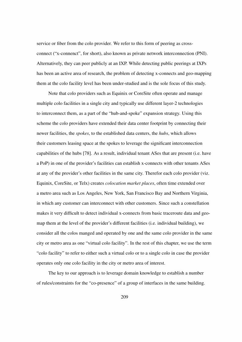
service or fiber from the colo provider. We refer to this form of peering as cross-
connect (“x-connenct”, for short), also known as private network interconnection (PNI).
Alternatively, they can peer publicly at an IXP. While detecting public peerings at IXPs
has been an active area of research, the problem of detecting x-connects and geo-mapping
them at the colo facility level has been under-studied and is the sole focus of this study.
Note that colo providers such as Equinix or CoreSite often operate and manage
multiple colo facilities in a single city and typically use different layer-2 technologies
to interconnect them, as a part of the “hub-and-spoke” expansion strategy. Using this
scheme the colo providers have extended their data center footprint by connecting their
newer facilities, the spokes, to the established data centers, the hubs, which allows
their customers leasing space at the spokes to leverage the significant interconnection
capabilities of the hubs [78]. As a result, individual tenant ASes that are present (i.e. have
a PoP) in one of the provider’s facilities can establish x-connects with other tenants ASes
at any of the provider’s other facilities in the same city. Therefor each colo provider (viz.
Equinix, CoreSite, or Telx) creates colocation market places, often time extended over
a metro area such as Los Angeles, New York, San Francisco Bay and Northern Virginia,
in which any customer can interconnect with other customers. Since such a constellation
makes it very difficult to detect individual x-connects from basic traceroute data and geo-
map them at the level of the provider’s different facilities (i.e. individual building), we
consider all the colos manged and operated by one and the same colo provider in the same
city or metro area as one “virtual colo facility”. In the rest of this chapter, we use the term
“colo facility” to refer to either such a virtual colo or to a single colo in case the provider
operates only one colo facility in the city or metro area of interest.
The key to our approach is to leverage domain knowledge to establish a number
of rules/constraints for the “co-presence” of a group of interfaces in the same building.
209

TABLE 14. Target CoreSite colos: their addresses, and the number of unique primaryASNs for tenants from CoreSite (CS), from PeeringDB (PDB), and their union (ASN).
Colo Address(es) CS PDB ASN
LA1/2One Wilshire /
290 217 444900 N Alameda St
CH1 427 S La Salle St 38 13 44MI1 2115 NW 22nd St 27 10 27
For instance, the very definition of an IP alias set implies that the group of interfaces
that comprises an alias set must be co-present in a colo facility. Then, we would like
to consider a collection of independent pieces of evidence to infer whether individual
interfaces are located at a specific facility. The key challenge in adopting this intuitive
strategy is that any individual instance of a co-presence rule/constraint is prone to error
(e.g. DNS misnaming of an interface results in it being geo-mapped to a different city).
This in turn could lead to the conflicting inference from different rules. More importantly,
conducting inference by iteratively applying these rules could easily magnify a seemingly
small error and render this approach useless.
To cope with these issues, we adopt a novel element for this problem in the form
of a probabilistic inference approach from a collection of independent and potentially
inconsistent pieces of evidence. In particular, we apply Belief Propagation algorithm
to perform inference on a Markov Random Field graphical model that is tailored to the
problem at hand. This probabilistic framework has the additional advantage that it can
be used as a starting point by anyone who may have more informative measurements
and/or access to better or improved heuristics that can be used to refine the underlying
graphical model (e.g. modify inter-dependencies by imposing tighter constraints). Over
time, incorporating such improvements can be expected to improve the completeness and
accuracy of this mapping effort to the point where the desired transparency in the ways
networks interconnect with one another becomes reality.
210

Localized Measurements
This section describes how we conduct purposefully designed data-plane
measurements in the form of traceroute probes such that they are more likely to pass
through (and thus reveal the presence of) a potential interconnect between a pair of
tenant ASes in our target facility. To maximize the likelihood of detecting possible
interconnects between tenants in a target facility with a limited number of measurements,
our probing strategy consists of the following three steps: (i) collecting publicly available
data about our target colo facility in full measure; (ii) selecting the source and destination
of traceroute probes to be as close to the facility as possible with respect to both network
and geographic distance; and (iii) launching probes in a criss-cross fashion to examine all
possible pair-wise interconnects between tenants of our target facility. We next describe
the first two steps steps in more detail.
Colocation Data Acquisition
Collecting publicly available information about a target colo facility includes
obtaining (i) the physical address of the facility, (ii) a list of customers (i.e. colo tenants),
and (iii) a list of partner IXPs that are reachable in the facility. For a given facility, to
capture a comprehensive list of tenants and partner IXPs, we use publicly available
information on different web sites (including those of the facility provider’s company, the
different tenants that publicize their presence in the facility, and third-parties that collect
some of this information) and supplement (and compare) it with similar information
provided by databases such as PeeringDB [211] that are maintained for the main purpose
of facilitating the exchange of information related to Internet interconnections (i.e.
peerings).
211

TABLE 15. Characteristics of vantage points and destination IPs selected for campaignsaround each colo
MI1 CH1 LA1/2IP AS IP AS IP AS
LG 24 21 23 22 95 77RIPE 10 6 24 16 47 21
Local IP 24 19 23 29 95 179Local Web 86 15 272 17 1,049 64Unseen AS 78 1 20 8 2,493 68
One complicating factor in acquiring colocation data is that many of the available
lists of tenants include the names of the different tenant networks/organization but don’t
provide the ASNs that these networks use to announce their routed prefixes. However,
to be able to identify possible interconnections in a target facility from traceroute
measurements, we need to be able to obtain the relevant ASNs for each of the facility’s
tenant. To this end, we combine various ASN-related information obtained from pulic
sources (such as Hurricane Electric BGP Toolkit [98], whois services, and AS-related
repositories maintained by CAIDA [52]) and infer for each tenant AS its primary ASN.
To identify the primary ASNs for each tenant network, we use AS relationship data from
CAIDA [53] and count the number of relationships between individual ASN and all other
ASNs associated with the customer list in a target facility. Then, for each tenant, we pick
the ASN(s) with the maximum number of relationships as the primary ASN(s) for the rest
of our analysis.
Table 14 summarizes the collected information about our target facilities, including
their street address and the number of primary ASNs for the list of tenants that we
obtained from CoreSite, PeeringDB and their union, respectively.
212

Source Selection
Our ability to effectively localize our probes depends primarily on having access to
vantage points (VP) at close-by locations. To address this issue, we leverage both Looking
Glasses and RIPE Atlas nodes.
Looking Glasses (LG)
Major ISPs usually offer a LG as a web-based front-end to one or more back-
end routers that allows a user to interactively run network debugging commands on the
back-end routers. The associated web page also provides the ASN and the city where
individual routers are located. Providers often enforce a tight rate-limit on their LGs’
usage which renders them unsuitable for large-scale measurement campaigns. Using a
list of 200+ LGs from traceroute repositories (e.g. [155]) and PeeringDB, we select the
sources for our traceroute probes as follows. First, we select those LGs that are within a
tenant AS; next, if no LG exists inside a given tenant AS, we look for LGs in its customer
cone and select the LGs with the shortest AS-hop distance. For these selected LGs, we
subsequently obtain their list of back-end routers and their locations. Given the list of
back-end routers associated with these selected close-by LGs, we select all that are inside
the city of our target colo. If no such VP is found, we pick one that is geographically
closest to the target facility. In our case studies, the median geo-distance of the selected
VPs/routers used for our measurement is less than 10 miles, and 95% of the routers are
within 1 000 miles of the target facilities.
RIPE Atlas
RIPE Atlas is a global network of remotely programmable probes that can launch
basic network measurements such as ping and traceroute. RIPE’s API allows one to
213

select probes in specific ASes (if there are any) that are within a certain geographic area.
This feature is ideally suited for our localized measurement, and we select all RIPE
probes that are within a 100-mile radius of the target colo regardless of their ASes and
use them to run Paris traceroute [23].
These two measurement infrastructures offer complementary views of the data-
plane. While LGs are usually located in major transit ASes and only very rarely in small
eyeball ASes, RIPE probes are typically found in eyeball ASes and less frequently in
transit ASes. The top part of Table 15 shows the number of tenant ASes in which we
have identified VPs from each platform, along with the total number of VPs for our target
facilities. LGs provide a desired vantage point in more tenant ASes than RIPE Atlas does.
Destination Selection
To increase the likelihood that our localized data-plane measurements traverse an
interconnection inside our target facility, we select destination IP addresses in the tenant
ASes and ensure the IPs are geolocated to the vicinity of the target colo. Specifically,
we rely on the following three sets of destination IPs for our localized traceroute
measurements.
Local IPs
Using a large pool of geo-located IP addresses collected from a few major P2P
applications [214], we look for an IP address within each of the tenant ASes that has the
shortest geo-distance from the target colo facility. If we do not find such an IP for a tenant
AS or if the obtained distance is found to be more than 100 miles from the target colo, we
examine the advertised /24 prefixes by that tenant AS, geolocate the prefixes, and select
the one with the shortest geo-distance from the colo facility. Similar to [234], to infer the
214

geographic location of individual IPs, we use the majority vote among different IP-geo
databases that include EdgeScape [17], MaxMind [185], and IP2Location [141]1. The
average distance of IPs in this pool from their corresponding target facility is between 40
to 75 miles for different campaigns, i.e. these destinations IPs are usually within the same
metropolitan area of the target facility.
Local Web Servers
Some colo customers provide web hosting services and use the colo facility to
house (parts of) their server farms. However, hosting providers also tend to distribute
their deployments in a few colo market places for fault tolerance and avoiding single point
of failure, therefore selecting a single IP in these ASes may not be sufficient. By targeting
the web services that they host, and are potentially deployed in our target colo, we should
be able to hit their interconnects with other tenant ASes in our target colo. Assuming
that local institutions (e.g. schools, local government agencies, and small businesses) are
likely to use these hosting providers, the web address of these institutions offer promising
local targets for our traceroute probes. To identify these local institutions, we crawl online
directories (e.g. Yelp, Google maps and Yellow Pages) and compile a list of their web
pages. We then look up the corresponding IP addresses and infer their geolocations and
their ASes (using Team Cymru IP-ASN service [250]2). We only select IP addresses as
destination IPs that belong to a tenant AS of the target colo and are geolocated within
a 50-mile radius of the facility. Our primary localized targeted measurements include
traceroutes from RIPE VPs to both local IPs and local web servers, and from LGs to local
1Unless stated otherwise, we always use the majority voting scheme throughout our work when geo-locating IPs using IP-geo databases.
2We primarily rely on Team Cymru IP-ASN service [250] to identify the ASN that advertises each IP
215

IPs. We then supplement these measurements with additional measurement as discussed
in the next section.
Unseen ASes
Irrespective of how we select VPs and/or destination IPs, our traceroute
measurements may fail to reveal some of the tenant ASes in the target facility. To detect
these “unseen ASes”, we use simple BGP-based IP-ASN mapping and rely on IP-geo
mapping. If for a tenant, no IP is found in the target city, it is marked as an unseen AS.
To discover the local footprint of these ASes, we conduct more comprehensive localized
data-plane measurements. Specifically, we identify all the /24 prefixes advertised by
each unseen AS, geo-locate the first IP in each prefix, and select all those IPs that are
within a 50-mile radius of our target colo as destinations for our probes. We supplement
the primary measurements with additional localized measurements obtained by running
traceroutes from the local RIPE VPs to the IPs associated with the “unseen ASes.”
The bottom part of Table 15 summarizes the number of tenant ASes for each
target colo in which we found at least one close-by destination IP using each of the three
discussed methods. Local IPs provide a desirable target in a majority of tenant ASes in
each of the target colos.
Inferring AS Interconnects
As a result of performing only localized measurements, we are able to significantly
limit the number of traceroute measurements that we exploit for mapping the x-
connects in a target facility. In total, we only ran 170K, 8K, and 2.5K traceroutes for our
measurement campaigns in LA, Chicago, and Miami, respectively. Moreover, we were
able to run all of these measurements in a single day, and repeated the data collection five
216
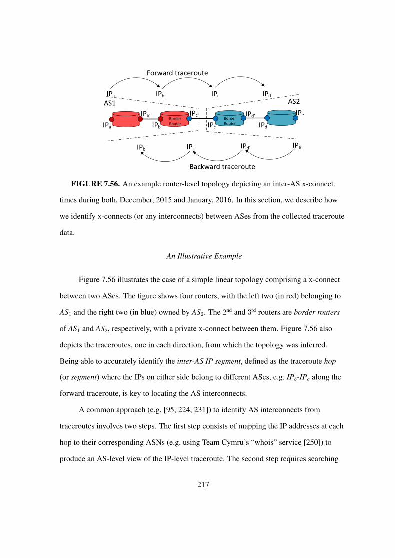
IPa IPb
IPb'
IPc
IPc'
IPd
IPd' IPe
AS1 AS2
Border Router
Border Router
IPb' IPc' IPd' IPe
IPa IPb IPc IPd
Forward traceroute
Backward traceroute
FIGURE 7.56. An example router-level topology depicting an inter-AS x-connect.
times during both, December, 2015 and January, 2016. In this section, we describe how
we identify x-connects (or any interconnects) between ASes from the collected traceroute
data.
An Illustrative Example
Figure 7.56 illustrates the case of a simple linear topology comprising a x-connect
between two ASes. The figure shows four routers, with the left two (in red) belonging to
AS1 and the right two (in blue) owned by AS2. The 2nd and 3rd routers are border routers
of AS1 and AS2, respectively, with a private x-connect between them. Figure 7.56 also
depicts the traceroutes, one in each direction, from which the topology was inferred.
Being able to accurately identify the inter-AS IP segment, defined as the traceroute hop
(or segment) where the IPs on either side belong to different ASes, e.g. IPb-IPc along the
forward traceroute, is key to locating the AS interconnects.
A common approach (e.g. [95, 224, 231]) to identify AS interconnects from
traceroutes involves two steps. The first step consists of mapping the IP addresses at each
hop to their corresponding ASNs (e.g. using Team Cymru’s “whois” service [250]) to
produce an AS-level view of the IP-level traceroute. The second step requires searching
217
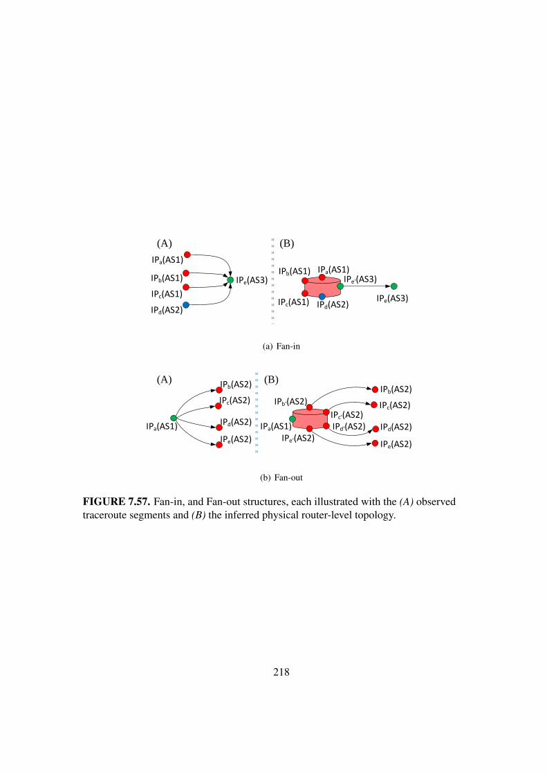
IPe(AS3)
IPa(AS1)
IPb(AS1)
IPc(AS1)
IPd(AS2)IPe(AS3)
IPa(AS1)IPb(AS1)
IPc(AS1) IPd(AS2)
IPe'(AS3)
(A) (B)
(a) Fan-in
IPb'(AS2)
IPc'(AS2)IPd'(AS2)
IPe'(AS2)IPa(AS1)IPa(AS1)
IPb(AS2)
IPc(AS2)
IPd(AS2)
IPe(AS2)
(A) (B)IPb(AS2)
IPc(AS2)
IPd(AS2)
IPe(AS2)
(b) Fan-out
FIGURE 7.57. Fan-in, and Fan-out structures, each illustrated with the (A) observedtraceroute segments and (B) the inferred physical router-level topology.
218

the obtained AS-level view to find adjacent hops with different ASes which is then
viewed as an indication of an interconnect between those ASes at that hop. Since the
IP-to-ASN mapping in step one is known to be error-prone ([63, 180, 138]), we take a
different approach and focus on the more challenging problem of inferring the inter-AS IP
segment in measured traceroutes.
What makes the task of accurately inferring the inter-AS IP segment corresponding
to a x-connect from traceroutes difficult is the required sharing of IP addresses between
two connected ASes [175, 32]. Specifically, the IP addresses on both ends of a x-connect
should be part of the same subnet, often a /30 or /31 subnet. This implies that of the two
parties (i.e. ASes) to a x-connect, one is supposed to allocate the IP addresses for both
interfaces of the x-connect at hand. What complicates the problem even further is the
fact that the nature or direction of shared IP addresses between two connected ASes is
generally unknown and could even vary across different x-connects on a single router.
Since the commonly-used approach described above is in general not capable of dealing
with these complications, alternative solutions or heuristics are needed.
To highlight this issue, consider Figure 7.56 where the interfaces on both ends of
the x-connect (IPc and IP′c) are allocated by AS2. A traceroute from AS1 to AS2 traverses
through IPa→ IPb→ IPc which identifies IPb–IPc as the inter-AS IP segment. However,
a traceroute in the reverse direction—IPd′ → IPc′ → IPb′—identifies an incorrect inter-AS
IP segment, namely IPc′–IPb′ . Similarly, the case where the VP from where traceroutes
are launched resides on a border router of, say, AS1, but the IP visited at the first hop
of the resulting traceroutes is in a different AS also causes problems and needs special
attention. To deal with such cases, we also consider the segment from the VP to the first
219

hop’s IP (i.e. the segment between hop0 and hop1)), representing the hop-zero segment to
be part of the traceroute.3
Inferring AS Owner of Border Routers
To tackle the problem of accurately inferring from traceroutes the inter-AS IP
segments corresponding to x-connects, we build on prior studies, especially [32] that
have proposed various heuristics to identify these inter-AS IP segments. However,
instead of tackling the problem directly, we change our focus and are explicitly interested
in systematically identifying the owner ASes of border routers. Once this ownership
is established, we can associate all interfaces of a border router with its owner AS,
regardless of their BGP-based mapping, and the sharing of IP addresses between (the
border routers of) any two ASes does therefore no longer complicate the task of inferring
the location of the x-connects between (the border routers of) these ASes. To solve this
new and previously largely ignored problem of inferring the AS ownership of border
routers, we describe below a number of old and new heuristics and illustrate how they
help us achieve our goal.
A Majority AS in an Alias Set
While “majority voting” is not a new heuristic, we include it here for completeness
and to illustrate its particular implementation for the problem at hand. To start, each alias
set that is identified by an alias resolution technique represents a subset of interfaces
associated with a router. Utilizing some conventional IP-to-AS mapping technique (based
on BGP information) for individual IPs in an alias set, we use a (conservative) majority
voting among the interfaces to determine the owner AS of the router. More specifically,
3We identified a substantial number of AS-links at hop-zero. For instance, in our LA campaign we find76 x-connects exclusively at hop zero.
220

given an alias set, we consider the corresponding router to belong to AS1 if the number of
interfaces in the set that are owned by AS1 is more than two-times plus one the number of
interfaces mapped to any other AS, i.e. a clear majority of interfaces are mapped to AS1.
This conservative majority criteria ensures that no owner is determined when the alias set
is small or does not have a dominant owner AS. In such cases, we call the corresponding
router “ambiguous” (i.e. its owner AS is not determined) and rely on other heuristics to
resolve the ambiguity.
Fan-in & Fan-out
To explain this new heuristic, consider a collection of inter-AS IP segments (with
two IPs, one on either side) from different traceroutes that either share the first or the
second IP (of the segment). We refer to these scenarios as fan-in, shown in Figure 7.57(a),
and fan-out, shown in Figure 7.57(b)). In these figures, the color of each IP address
denotes the AS that advertises the IP and the color used for routers indicates the owner
AS of the router.
In the absence of layer-2 switches along the path, a plausible router-level topology
that is consistent with all these inter-AS IP segments is shown on the right-hand side of
Figure 7.57(a) for fan-in and on the right-hand side of Figure 7.57(b) for fan-out. In the
case of fan-in, a router-level is plausible if it satisfies the condition that the first hops of
all inter-AS segments in a fan-in scenario (e.g. IPa through IPd in Figure 7.57(a)) form
an alias set. In the case of fan-out, the condition is that for each second hop in a fan-out
scenario, there is an IP address from the same subnet (thus owned by the same AS) that
is a member of an alias set with the first hop IP address. Once such alias sets are inferred,
we apply our conservative majority voting heuristic to determine the owner AS of the set
or label the router as “ambiguous.”
221
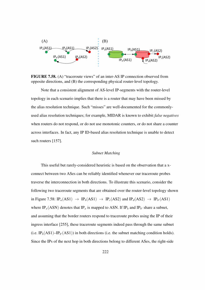
IPa(AS1) IPc(AS2)
IPd(AS2)
IPb(AS1)
IPb'(AS1)
(A) (B)
IPa(AS1)
IPd(AS2)
IPb(AS1)
IPb'(AS1)IPc(AS2)
IPc'(AS2)
FIGURE 7.58. (A) “traceroute views” of an inter-AS IP connection observed fromopposite directions, and (B) the corresponding physical router-level topology.
Note that a consistent alignment of AS-level IP-segments with the router-level
topology in each scenario implies that there is a router that may have been missed by
the alias resolution technique. Such “misses” are well-documented for the commonly-
used alias resolution techniques; for example, MIDAR is known to exhibit false negatives
when routers do not respond, or do not use monotonic counters, or do not share a counter
across interfaces. In fact, any IP ID-based alias resolution technique is unable to detect
such routers [157].
Subnet Matching
This useful but rarely-considered heuristic is based on the observation that a x-
connect between two ASes can be reliably identified whenever our traceroute probes
traverse the interconnection in both directions. To illustrate this scenario, consider the
following two traceroute segments that are obtained over the router-level topology shown
in Figure 7.58: IPa(AS1) → IPb(AS1) → IPc(AS2) and IPd(AS2) → IPb′(AS1)
where IPx(ASN) denotes that IPx is mapped to ASN. If IPb and IPb′ share a subnet,
and assuming that the border routers respond to traceroute probes using the IP of their
ingress interface [255], these traceroute segments indeed pass through the same subnet
(i.e. IPb(AS1)–IPb′(AS1)) in both directions (i.e. the subnet matching condition holds).
Since the IPs of the next hop in both directions belong to different ASes, the right-side
222

router must be owned by AS2 and therefore the link IPb(AS1)–IPb′(AS1) is the x-connect
between these two ASes. Indeed this implies that IPd(AS2) and IPb(AS1) are part of an
alias set, but failed to be identified as such by the alias resolution technique.
To apply this heuristic, we use XNET [255] to identify all IP address pairs that are
on the same subnet. Among the IP-segments from AS1 to AS2 and the reverse direction,
we examine whether the far-side of one inter-AS IP segment (IPb′(AS1)) is in the same
subnet as the near-side of another IP-segment (IPb(AS1)) in the reverse direction. If this
condition is satisfied, we then set the owner AS of the near-side (IPb) to be AS2 instead of
AS1.
Sink IPs
Another original heuristic is based on the empirical observation that traceroutes
that are destined toward small regional tenant ASes reveal two common patterns. For
one, many such traceroutes terminate at a specific set of IP addresses, referred to as sink
IPs, before they reach the destination AS. In addition, these sink IP addresses are never
encountered in traceroutes toward other ASes. The observed strong association between
small regional ASes and sink IPs suggests that these sink IPs indeed reside on a router
that is owned by the regional AS.
To validate this heuristic, we manually examined more than 500 sink IPs and
observed that while the PTR record (DNS name) of a sink IP has a domain that
matches the AS that advertises the IP address through BGP, the name also tends to
contain hints that point to the regional AS. For instance, the sink IP for Televergence
Solutions Inc. (AS30188) is advertised by GTT (AS3257) and its DNS name is
televergence-gw.ip4.gtt.net. Thus, instead of relying on inaccurate BGP-based AS
223
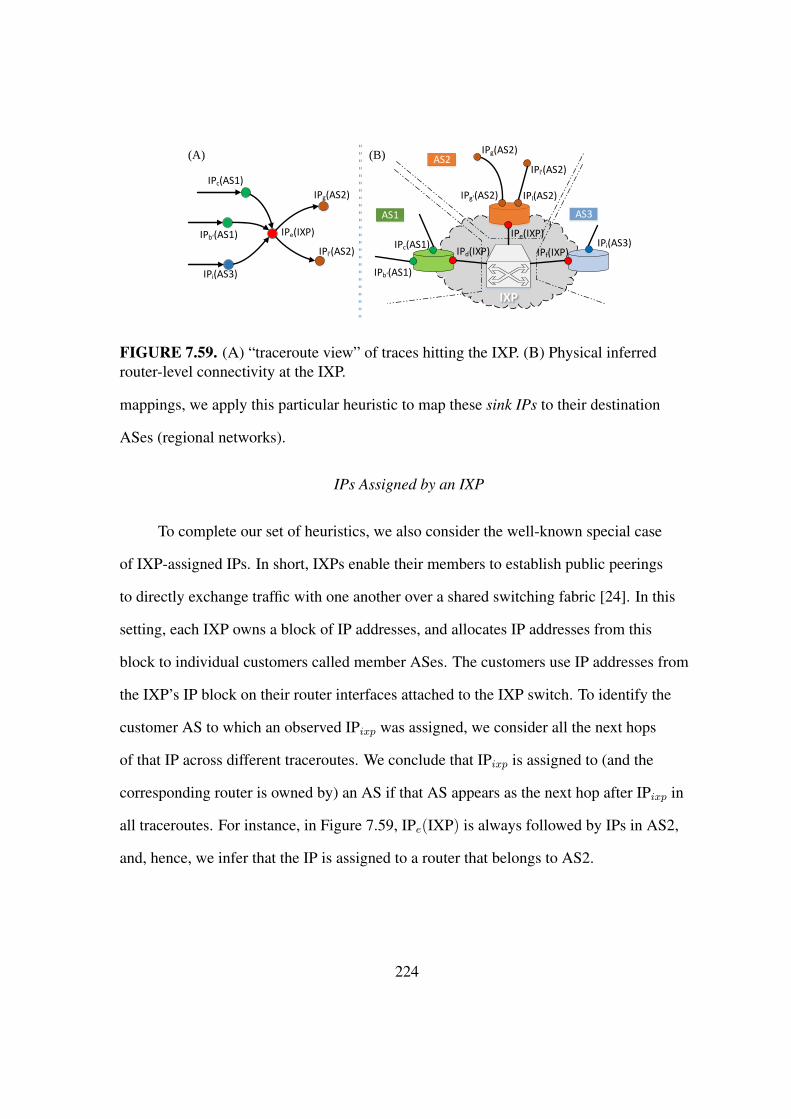
IPb'(AS1)
IPc(AS1) IPd(IXP)
IPe(IXP)
IPf(IXP)
IPg(AS2)
IPg'(AS2)
IPi(AS3)
IPl(AS2)
IPl'(AS2)
AS1 AS3
IXP
AS2
IPg(AS2)
IPl'(AS2)
IPc(AS1)
IPi(AS3)
IPe(IXP)IPb'(AS1)
(A) (B)
FIGURE 7.59. (A) “traceroute view” of traces hitting the IXP. (B) Physical inferredrouter-level connectivity at the IXP.
mappings, we apply this particular heuristic to map these sink IPs to their destination
ASes (regional networks).
IPs Assigned by an IXP
To complete our set of heuristics, we also consider the well-known special case
of IXP-assigned IPs. In short, IXPs enable their members to establish public peerings
to directly exchange traffic with one another over a shared switching fabric [24]. In this
setting, each IXP owns a block of IP addresses, and allocates IP addresses from this
block to individual customers called member ASes. The customers use IP addresses from
the IXP’s IP block on their router interfaces attached to the IXP switch. To identify the
customer AS to which an observed IPixp was assigned, we consider all the next hops
of that IP across different traceroutes. We conclude that IPixp is assigned to (and the
corresponding router is owned by) an AS if that AS appears as the next hop after IPixp in
all traceroutes. For instance, in Figure 7.59, IPe(IXP) is always followed by IPs in AS2,
and, hence, we infer that the IP is assigned to a router that belongs to AS2.
224

TABLE 16. Details on heuristics used in each campaign
Miami Chicago Los Angeles
Alias sets 576 738 3644IPs in alias sets 3279 3996 22573
Alias sets with majority 512 645 3074
Fan-in 336 370 4023IPs in fan-in 658 696 6441
IPs fan-in with majority 404 401 3823
Fan-out 285 366 3125IPs in fan-out 362 473 4122
IPs fan-out with majority 215 226 2278
Sink IP 284 475 3063
Resolved IXP IP 26 43 420
Subnets matched IP 10 16 180
Evaluation of our Heuristics
To evaluate the effectiveness of the different heuristics, we consider all of our
collected traceroute measurements and give in Table 16 a detailed account of how the
heuristics performed for each of our measurement campaigns.
We use MIDAR [157] to identify all alias sets that belong to the same router in
order to apply the majority voting heuristic among all the IPs that traceroutes visited. As
the input to alias resolution, we consider the union of two sets S1 and S2 of IP addresses
in a measurement campaign; S1 is the set of IP addresses observed in the traceroutes and
S2 denotes the set of IP addresses in /30 subnets of the IPs in S1. Including the set S2
allows us to identify more IPs from each alias set due to IP sharing. The top portion of
Table 16 shows, for each campaign, the number of identified alias sets, the counts of IPs
in these sets, and the number of alias sets where our conservative majority voting scheme
identifies an owner. Such an owner is identified for 83-88% of alias sets. 2-4% of the
IP addresses in the discovered alias sets (when the scheme identifies an owner AS) are
225

inferred to be on routers that do not belong to the AS that advertises them via BGP. The
second and third portions of Table 16 reports the same quantities for our fan-in and fan-
out heuristics. The bottom portion of the table gives the number of IPs that result from
applying the subnet matching, sink IP, and IXP-assigned IP heuristics, respectively, for
each of our campaigns.
Where our heuristics have insufficient evidence to reliably infer the owner AS of a
router and therefore label that router as “ambiguous”, we apply an additional heuristic
(here called the “valley-free heuristic”) that leverages commonly used control plane
information in the form of inferred AS relationships (e.g. [53]). Specifically, we consider
all traceroutes that pass through an interface, say IPx, of an ambiguous router (i.e. IPx
represents an IP from the relevant alias set) and focus on the AS-level view of the three
hop segment containing the hop before and after IPx. We then iterate through the list of
potential owner ASes of IPx and check each time whether the resulting AS-level path
segment is indeed valley-free. A valley-free route is one in which the transit AS is not the
customer of either ASes connected by the transit provider. Any candidate AS that results
in a valley-free AS-level segment in all traceroutes is considered as a viable owner for this
particular ambiguous router. In our data where we encounter more than 400 ambiguous
routers, we identify a single AS owner in 90% of the cases using this valley-free heuristic.
Note that once we identify the owner AS of a router, we assign all IPs in the alias
set to the owner AS (of the router). Some of these IPs may have been originally mapped
to a different AS (e.g. based on BGP advertisements), and these IPs are now reassigned to
the owner AS. We observe such IP-to-AS reassignments for 10-15% of all observed IPs
in each measurement campaign and different heuristics contribute between 5-35% to the
226

TABLE 17. Percentage of IPs reassigned to owner ASes of routers by different heuristicsin each campaign.
Miami Chicago Los Angeles
Alias 23.00 14.60 16.91IXP 8.67 13.35 13.33Sink 24.33 35.40 32.55
Fan-in 20.67 17.08 18.78Fan-out 36.33 28.57 36.48
Subnet Match 3.33 4.04 2.66
Valley Free 16.00 18.32 15.04
reassignments. Table 17 shows the percentages4 of IPs that get reassigned to a different
AS by the different heuristics in each measurement campaign.
We validate this router-aware IP-to-AS mapping heuristic using two different data
sources. For one, we use information published by IXPs and PeeringDB to validate the
owner AS of IXP-assigned IP addresses inferred through our heuristics. We observe
that more than 92% of the inferred owner ASes for IXP-assigned IPs are consistent with
this public information. Second, we use hints embedded in DNS names that suggest IP
address sharing between two ASes. A DNS naming convention used by some ASes (e.g.
Level3, GTT, NTT and PCCW) is to embed the name of the peer AS in the DNS name
for the IP address used to establish the peering link. For this type of validation, we focus
on the IP addresses that our heuristics mapped to an AS other than the BGP-based owner
AS. For example, in the case of ae-0.teliasonera.chcgil09.us.bb.gin.ntt.net we
check to see if the IP address is inferred to be assigned to AS1299 (i.e. TeliaSonera). Out
of nearly 4K such IP addresses that we examined, some 25% have a valid DNS name,
and about 40% of these names explicitly indicated IP address sharing. More than 90%
4The sum of percentages along a column can be more than 100% as multiple heuristics may suggest thesame remapping.
227

TABLE 18. Aggregation guidelines
(I) Fan-in aggregation
Near-side Far-side
141.136.106.153 → 63.218.42.589.149.130.129 → 63.218.42.5141.136.106.157 → 63.218.42.5141.136.106.161 → 63.218.42.5141.136.106.5 → 63.218.42.5141.136.111.205 → 63.218.42.589.149.129.121 → 63.218.42.5
(II) Subnet matching aggregation
Near-side Far-side
141.136.106.153 → 63.218.42.563.218.42.129 → 63.218.42.6
of the hints extracted from the DNS names match the router owner AS inferred by our
heuristics5.
Accurate AS Interconnect Counting
An important implication of accurately inferring the owner AS of border routers
is that the resulting router-level view allows for a more accurate accounting of the actual
number of x-connects encountered in traceroutes. For example, the fan-in scenario in
Figure 7.57(a) clearly shows that there is a single x-connect between the two ASes;
simply counting inter-AS IP segments in different traceroutes [95, 224, 115] would result
in over-counting x-connects.
The following two guidelines are concerned with properly aggregating different
views of a single x-connect between a pair of ASes.
5We provide the list of all the remapped IP addresses with the associated PTR record throughthe following online tables: onrg . cs . uoregon . edu / impact / resources / router -asn/validate/
228

Fan-in Aggregation: Motivated by the fan-in scenario illustrated in Figure 7.57(a),
this guideline advises to aggregate all the observed AS-level IP segments or interconnects
that have the same far-side IP address and consider them as different views of the same x-
connect in the same direction. For instance, Figure 7.57(a) shows 7 inter-AS IP segments,
but we count them as only one x-connect.
Subnet Matching Aggregation: This guideline is motivated by our subnet
matching heuristics. It suggests aggregating all the discovered AS-level IP segments
whose far-side IP addresses are used for the two ends of an interconnection and consider
these segments as different views of one and the same x-connect in opposite directions
(See Figure 7.58). Table 18(II) shows an example case with 2 inter-AS IP segments that
are counted under this guideline as a single x-connect since the far-side IP addresses
belong to a /31 subnet and therefore are two ends of one interconnection.
Note that these guidelines can be used in combination as well. As our examples in
Tables 18(I) and 18(II) demonstrate, all the AS-level IP segments in the two examples
can be aggregated to a single x-connect between AS3257 and AS3491. To illustrate the
practical relevance of these aggregation guidelines for properly accounting for the actual
number of x-connects in a target facility, the median number of aggregated views across
our measurement campaigns is 2, but we encountered cases were as many as 40 different
views were aggregated to yield a single x-connect.
Pinning X-Connects to Facilities
Equipped with the ability to infer x-connects between the owner AS of border
routers from our localized traceroute measurements, in this section we describe our
strategy for determining whether those x-connects can be mapped to the inside or outside
of our target facility. This “pinning” process consists of considering the interface IPs
229

on both sides of the inferred AS interconnections, identifying a set of “anchors” (i.e.
interfaces that can be reliably mapped to the inside or outside of the target facility),
and then performing belief-propagation-based inference on a purposefully constructed
graphical model. This model reflects our best efforts described in Sections 7.3 and 7.4
at inferring an underlying router-level connectivity structure surrounding the target
facility that is as consistent as possible with the comprehensive view derived from all
our traceroute measurements. In this section, we describe this pinning process in more
detail.
Pinning Process: Anchors
We start by selecting all the observed IP addresses in a measurement campaign
for which we have any clues that they may be located in the target colo. To identify this
“relevant” pool of IP addresses for pinning, we first remove all IP addresses that are
associated with routers owned by ASes that are not tenants in the target facility. Next,
we eliminate all the observed IP addresses in a measurement campaign for which we
cannot find any evidence that they are geo-located to the target city. To this end, we
remove all interfaces associated with any alias set if geo-location hints in all their PTR
records (when available) indicate a location other than the target city. We also remove any
interface that is not mapped to the target city by any of the IP-geo mapping databases (see
Section 7.3). Any remaining IP address is included in the relevant pool and considered for
pinning.
To bootstrap the pinning process, we rely on a set of anchors that can be reliably
mapped to the inside or outside of our target colo. For determining which subset of the
“relevant” pool of IP addresses can serve as reliable inside/outside anchors, we examine
230
the relevant pool of IP addresses for the following three types of solid location-specific
evidence:
Facility Information in DNS Names: Some networks encode specific information
about the colo that hosts their deployment site in PTR records (DNS names). This in turn
provides reliable information about the interface location at the facility level. Examples
for such encodings include rt0as-equinix.vx.shawcable.net which clearly suggests
deployment in an Equinix colo or as22822-9.111eighthave.ny.ibone.comcast.net
which reveals the address of the facility to be 111, 8th ave, NYC, which is a well-known
major Internet hub in NYC. We rely on our in-house DNS parser (i.e. ALFReD [194]) to
detect and extract any such hints from the PTR records of relevant interfaces.
IPs co-located with IXPs: Publicly-available partnerships between IXPs and colos
(e.g. Any2 IXPs and CoreSite) offer additional specific evidence for identifying IP
addresses that are located inside a colo. For one, individual IXPs have their own dedicated
and well known IP prefixes from which they assign an address (IPixp) to the interface
of a member’s router that connects to the IXP switching fabric [24]. Unless the IXP
partners with other colo facility providers, all these IPs are clearly located in the colo of
interest.6 Second, any IP address that is observed on a traceroute prior to the IP from the
partner IXP’s prefix should also be located in the same colo [115]. To explain, consider
a traceroute segment with the consecutive 3 hops IPa(AS1) → IPIXP → IPb(AS2)
that belong to AS1, IXP and AS2, respectively. If AS1 is a member of the IXP and is
only present in the target colo facility, we conclude that IPa must be located inside the
same facility. Note that we cannot reliably draw the same conclusion for IPb that is
attached to the next-hop router [115]. Furthermore, an IXP partnering with other colo
6Some of the larger IXPs typically partner with multiple colo facilities e.g. www.laiix.net.
231

facility providers in the same city helps identify anchors that are located outside our target
facility.
Using Small Regional ASes: The presence of small regional ASes at a colo provides a
good opportunity for identifying anchors at that facility or validating already discovered
anchors. For economic reasons, a small regional tenant AS is most likely to have its
PoP only in a single colo in that city where it establishes all its interconnects. In fact,
presence in colos of different providers in the same city is proportionally more costly
and unnecessary for a small regional AS that typically deals with limited traffic volume.
We consider all observed IPs (including any LG) associated with such small regional
ASes to be located in the same colo facility. More formally, we use CAIDA’s AS rank
data [52] and consider a tenant AS to be a small regional AS if it has less than 5 ASes
in its customer cone and advertises less than 50 /24-prefixes. We also cross check any
selected regional ASes with PeeringDB to ensure that they do not have deployment sites
at multiple colos in the metro area of our target facility. Note that this evidence only
provides anchors inside the target facilities.
Table 19 presents the number of in/out anchors that we identified using each of
these three techniques in each one of the target cities. The number and relative fraction of
in/out anchors in each campaign depends on various factors including the number of colo
facilities in the target city and the number of tenant ASes in the target colo.
Pinning Process: Graphical Model Construction
We first present a set of domain knowledge-based co-presence rules/constraints that
indicate whether a group of interfaces is (or is not) co-located in the same colo facility.
We then construct a Markov Random Field (MRF) graphical model to encode all these
association rules/constraints along with their level of strength/certainty. The resulting
232

TABLE 19. The number of in- and out-anchors identified by the individual techniques foreach target colo facility
Miami Chicago Los AngelesIN OUT IN OUT IN OUT
DNS hints 0 21 0 40 3 43Small regional AS 11 0 126 0 336 0IXP 0 5 2 18 153 37IXP near-side 0 2 1 9 85 27
model serves as input to a probabilistic algorithm to determine whether individual IP
addresses are mapped inside or outside of the target facilities in a city.
Defining Co-presence Rules: We consider the following rules (or associations) that will
later on aid in the (probabilistic) inference of the co-presence of a group of interfaces in a
colo. These rules are ordered based on the level of confidence in their outcome (from low
to high).
1. Intra-domain links: The presence of two adjacent IPs from the same AS (i.e. intra-
domain IP-segment) on a traceroute with a very short RTT difference hints at co-
location of the IPs. The likelihood of co-location is inversely proportional to the
RTT difference.
2. Inter-domain Links: Similar to the previous case, the existence of two adjacent
IPs from different ASes (i.e. inter-domain IP segment) on a traceroute suggest that
the IPs are co-located. The likelihood of co-location is higher for interconnects
compared to intra-domain IP segments, since remote AS peering is often times
avoided for economical reasons. Note that in our case studies we require the
difference in RTT delays to be no more than 30ms to imply even the weakest
likelihood of co-presence.
233

3. PoP-Tag Rules: Among a number of operators, it is common practice to use DNS
naming conventions that embed a city name (or code) concatenated with numerical
values as a “PoP-tag” to distinguish interfaces associated with individual PoPs in a
metro area. For example, the DNS name for all interfaces associated with a specific
PoP of Level3 in Seattle has the format *.seattle1.Level3.net. We extract these
PoP-tags (in the form of Level3.net:seattle1) from DNS names and leverage
them to define the following two rules: (i) All interfaces of a tenant AS of a colo
facility that are associated with the same PoP-tag must be located in that same
colo facility. (ii) Two IPs of one and the same tenant AS of a colo facility that are
associated with different PoP-tags must be located in different colo facilities.
4. Alias Association: All interfaces in an alias set belong to a single router and must
therefore be co-located in the same colo facility.
Graphical Model Construction: We examine the “relevant” pool of interfaces derived
from a measurement campaign against our co-presence constraints and identify any
group of interfaces that satisfy any of these constraints. Then, we use a graphical
model of the Markov Random Field (MRF) type [158, 174] to encode all the observed
instances of individual co-presence constraints as an undirected graph. MRF is a
mathematical framework that is particularly well suited for solving inference problems
with uncertainty in observed data. We represent each interface as a node in the graph
and its association with other interfaces are encoded as edges with the proper weight (i.e.
level of confidence) between them. For instance, each instance of an alias or PoP tag
association rule is represented as a star-shaped graphlet where all relevant interface nodes
connect to the “association type” node in the center. Each node can be in a finite number
of states that statistically depend only upon the state of its neighbors. The probabilistic
independence of non-neighboring nodes is a key requirement for the applicability of234

TABLE 20. Sample propagation matrices for association and disassociation, ε < ϕ
(a) Association
V1 V2 φ P0 0 ε+ ϕ ε+ϕ
4ε+2ϕ
0 1 ε ε4ε+2ϕ
1 0 ε ε4ε+2ϕ
1 1 ε+ ϕ ε+ϕ4ε+2ϕ
(b) Disassociation
V1 V2 φ P0 0 ε+ ϕ ε+ϕ
4ε+3ϕ
0 1 ε+ ϕ ε+ϕ4ε+3ϕ
1 0 ε+ ϕ ε+ϕ4ε+3ϕ
1 1 ε ε4ε+3ϕ
the MRF model; That is unrelated nodes in an MRF (i.e. interfaces for which there is
no joint probability distribution on their location) have independent random variable
(conditioned over the location rest of the nodes). This essentially means that if two IPs
are a) not aliases, b) have not been seen in an IP-segment, or c) do not have similar PTR,
knowing the location of one does not affect our belief about the location of the other.
In our MRF model, we assign a binary random variable to each node. The two
states of IN and OUT indicate whether the node is inside or outside the colo (i.e. P (n =
IN) = 1 - P (n = OUT)), respectively. The state of each inside (outside) anchor node
is set to 1 (0). The joint probability distribution between all connected pairs of nodes
is represented by a Propagation Matrix, where entry (i, j) equals the probability (i.e.
based on the relative confidence of the constraint) of a node being in state j given that its
neighbor is in state i. A desired feature of MRF is its ability to effectively encode both
association and disassociation between nodes, i.e. whether two nodes must have similar or
opposite states. More specifically, for a pair of connected nodes, v1 and v2, we can define
the joint probability for each one of the four possible states. As shown in Table 20, a co-
presence association (e.g. being in an alias set) is encoded by assigning high probability
to similar states (e.g. (v1 = 0) ∧ (v2 = 0)) and low probability to opposite states (e.g.
(v1 = 1) ∧ (v2 = 0)). Conversely, disassociation (e.g. different PoP tags) requires the
235

84868890929496
% A
nch
or
inAnchor in & hit(BP)
2468
10121416
% A
nch
or
out
Anchor out & hit(BP)
1 2 3 4 5 6 7 8 9 100.5
1.0
1.5
2.0
2.5
3.0
% A
nch
or
in
Anchor in & miss(BP)
1 2 3 4 5 6 7 8 9 1060657075808590
% A
nch
or
out
Anchor out & miss(BP)
(a) Los Angeles; Test and validate to find the proper c
405060708090
100
% A
nch
or
in
Anchor in & hit(BP)
0.060.040.020.000.020.040.06
% A
nch
or
out
Anchor out & hit(BP)
1 2 3 4 5 6 7 8 9 100
5
10
15
20
25
% A
nch
or
in
Anchor in & miss(BP)
1 2 3 4 5 6 7 8 9 10949596979899
100
% A
nch
or
out
Anchor out & miss(BP)
(b) Chicago; Test and validate to find the proper c
FIGURE 7.60. The effect of c on i) the inferred believes about the anchors not used inBP; 40% anchors used in BP, and ii) the distribution of believes for all nodes.
opposite assignment of probabilities (Table 20). Note that the model allows two PoP-tags
of a network to be both OUT.
The joint probabilities are defined based on two parameters: ϕ is the main
parameter as ε is often set to a small value (0.05). In theory, a large training set should
be used to “learn” the value of ϕ. However, for our problem, this approach is not feasible.
Instead, we take a more pragmatic approach and argue that as long as the joint probability
for each co-presence constraint captures the relative ranking of our level of confidence
associated with these constraints, a probabilistic inference technique properly pins
individual interfaces without being too sensitive to the value of ϕ. In fact, the insensitivity
to the value of ϕ implies that the inferred solutions represent a basic pattern that is not an
artifact or side-effect of a specific parameter setting. We enforce the relative ranking of
the above-defined co-presence constraints by setting ϕ = k × c, where k is the order of a
co-presence constraint based on our level of confidence, i.e. the higher the confidence, the
larger the value of k. Therefore, c is a parameter that defines the relative gap/difference
between the value of ϕ for two adjacent constraints.
236
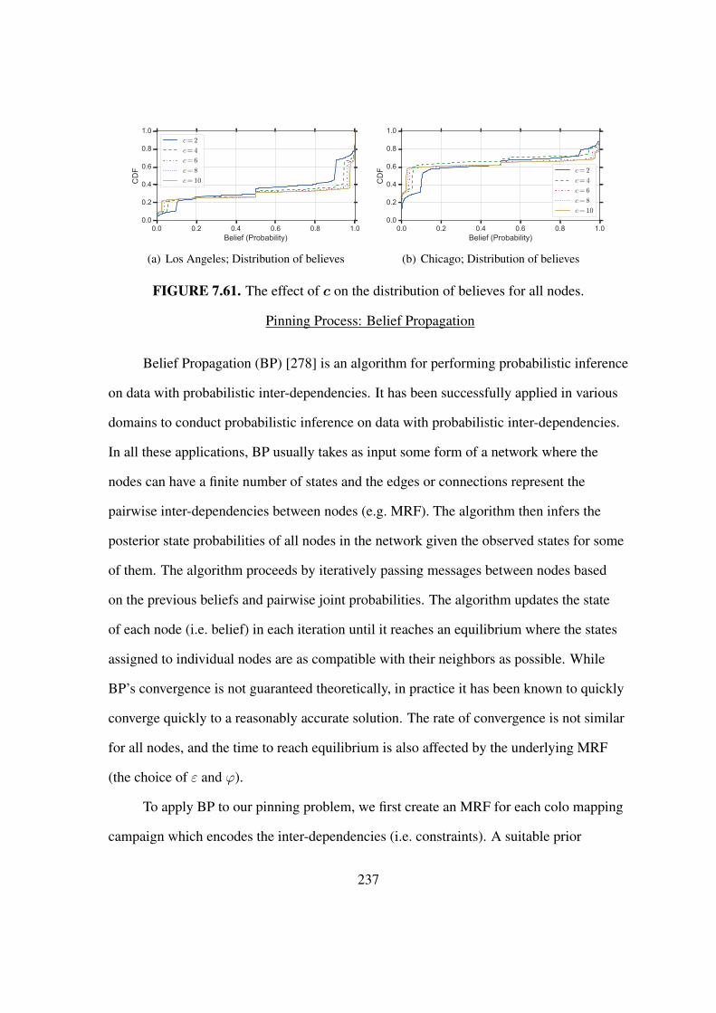
0.0 0.2 0.4 0.6 0.8 1.0Belief (Probability)
0.0
0.2
0.4
0.6
0.8
1.0C
DF
c= 2
c= 4
c= 6
c= 8
c= 10
(a) Los Angeles; Distribution of believes
0.0 0.2 0.4 0.6 0.8 1.0Belief (Probability)
0.0
0.2
0.4
0.6
0.8
1.0
CD
F c= 2
c= 4
c= 6
c= 8
c= 10
(b) Chicago; Distribution of believes
FIGURE 7.61. The effect of c on the distribution of believes for all nodes.
Pinning Process: Belief Propagation
Belief Propagation (BP) [278] is an algorithm for performing probabilistic inference
on data with probabilistic inter-dependencies. It has been successfully applied in various
domains to conduct probabilistic inference on data with probabilistic inter-dependencies.
In all these applications, BP usually takes as input some form of a network where the
nodes can have a finite number of states and the edges or connections represent the
pairwise inter-dependencies between nodes (e.g. MRF). The algorithm then infers the
posterior state probabilities of all nodes in the network given the observed states for some
of them. The algorithm proceeds by iteratively passing messages between nodes based
on the previous beliefs and pairwise joint probabilities. The algorithm updates the state
of each node (i.e. belief) in each iteration until it reaches an equilibrium where the states
assigned to individual nodes are as compatible with their neighbors as possible. While
BP’s convergence is not guaranteed theoretically, in practice it has been known to quickly
converge quickly to a reasonably accurate solution. The rate of convergence is not similar
for all nodes, and the time to reach equilibrium is also affected by the underlying MRF
(the choice of ε and ϕ).
To apply BP to our pinning problem, we first create an MRF for each colo mapping
campaign which encodes the inter-dependencies (i.e. constraints). A suitable prior
237

belief/state for anchor nodes is initially set to be inside or outside the target facility. We
then run the BP algorithm until 90% of the nodes reach a steady state. The outcome of the
algorithm shows the probabilistic beliefs about the location of each node. We divide the
location of nodes into three sets based on their resulting probability: (i) hit: stable nodes
whose probability to be in the target facility is more than 90%. (ii) miss: stable nodes
whose probability to be in the target facility is less than 10%. (iii) close call: the rest of
the nodes including those that did not reach an equilibrium.
We use a common test/validation technique to assess the sensitivity of BP’s
outcome to the value of c. We remove 10% − 60% of randomly selected anchors for
testing, and run the BP algorithm with the remaining anchors. We repeat each test 10
times using different random sets of anchors. As an example, consider the case where
the goal is to maximize the number of correctly inferred inside/outside anchors for
our measurement in LA using 40% of anchors for testing. The left-side plots in Figure
7.60 (from top to bottom) show the summary distribution of the fraction of test anchors
inside the target facility in LA that are mapped as hit,close-call or miss, as a function
of c. The right-side plots show the same information for test anchors outside the target
facility in LA. These results demonstrate that once the value of c exceeds 3 or 4, more
than 94% of inside anchors are correctly mapped and the variations across different runs
is very small. The mapping accuracy for outside anchors is around 82% and exhibits a
somewhat larger variability. Given the significantly smaller fraction of outside anchors
in LA, the relatively lower accuracy in mapping outside interfaces is not surprising. This
examination suggest that for c-values between 4 and 9, the BP algorithm results in the
highest level of accuracy.
This examination suggest that for c-values between 4 and 9, the BP algorithm
results in the highest level of accuracy. To offer more insight into the choice of c on
238

the outcome of BP algorithm, Figure 7.61 presents the inferred distribution of belief
probabilities for all nodes when running the BP algorithm with different values of c. This
results illustrate that the probability distribution quickly become bimodal as we increase
c. This implies that the inferred probabilities represent a basic pattern in the data that is
not an artifact of the choice of c or of the selected thresholds for defining hits and misses.
Pining Results
To demonstrate the applicability and feasibility of our pinning process for mapping
AS interconnections or peerings inside a target colo, we present the results of pining
for three CoreSite colos in Los Angeles, Chicago, and Miami, respectively. Table 21
summarizes the total number of nodes of each kind in our MRF framework and gives
the breakdown of their pinning to inside and outside of the colos. Table 22 shows the
number of IP-level interconnects where both ends are mapped to the target colos with
their breakdown between private and public in each target facility. Finally, we apply the
two aggregation guidelines alluded to in Section to avoid over-counting the number of
physical x-connects between two AS. The bottom row of Table 22 presents the number of
consolidated x-connects in each facility and shows that the number of physical x-connects
is two to four times smaller than the number of IP-level interconnects before aggregation.
Validation & Comparison
Colocation facility providers in general are not willing to disclose information
regarding interconnectivity of their tenant ASes, and our attempts at obtaining such
information from some colo providers were futile as well. In addition, tenant ASes
themselves are reluctant to share the details of their interconnectivity with other ASes,
unless they are sufficiently coarse so as to not reveal the type, precise location, and name
239
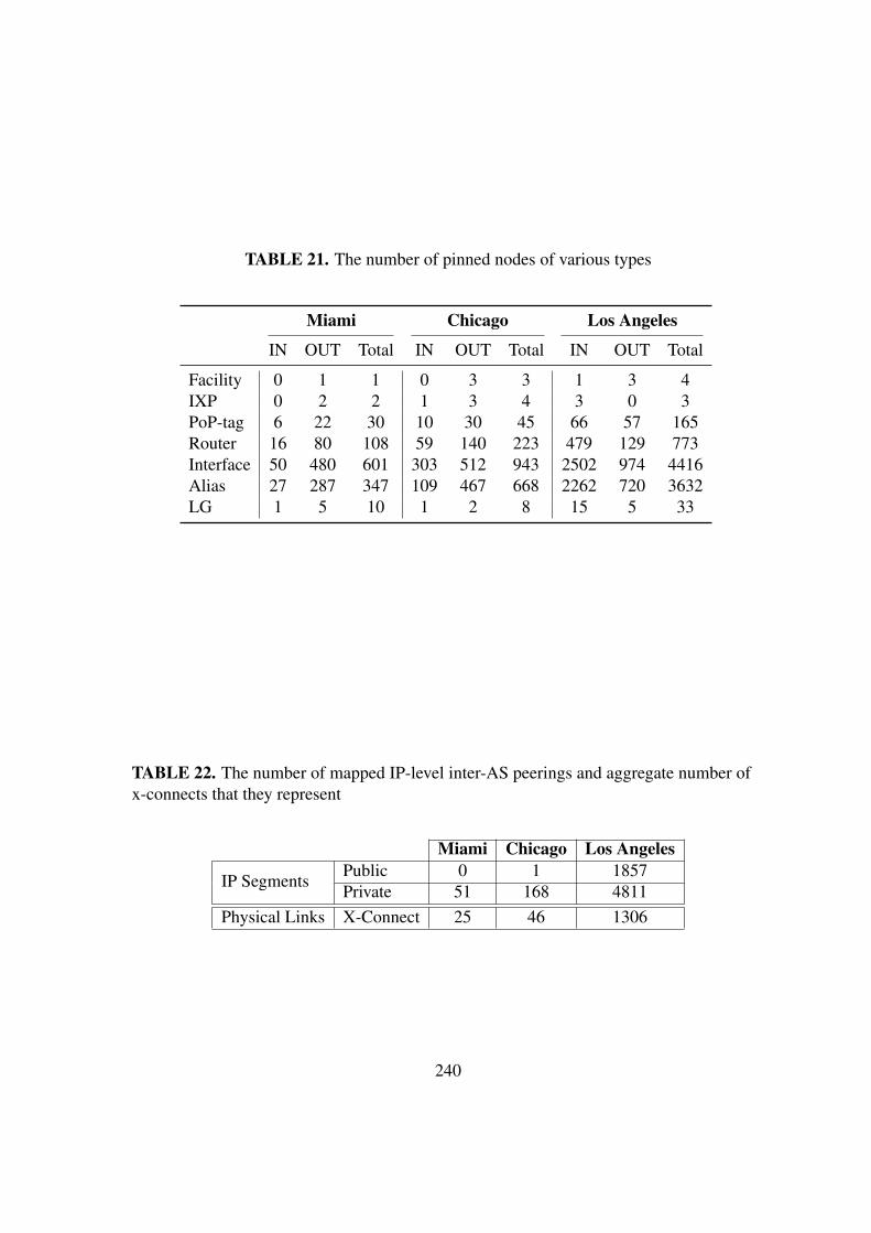
TABLE 21. The number of pinned nodes of various types
Miami Chicago Los Angeles
IN OUT Total IN OUT Total IN OUT Total
Facility 0 1 1 0 3 3 1 3 4IXP 0 2 2 1 3 4 3 0 3PoP-tag 6 22 30 10 30 45 66 57 165Router 16 80 108 59 140 223 479 129 773Interface 50 480 601 303 512 943 2502 974 4416Alias 27 287 347 109 467 668 2262 720 3632LG 1 5 10 1 2 8 15 5 33
TABLE 22. The number of mapped IP-level inter-AS peerings and aggregate number ofx-connects that they represent
Miami Chicago Los Angeles
IP SegmentsPublic 0 1 1857Private 51 168 4811
Physical Links X-Connect 25 46 1306
240

of the peer of an interconnection [103]. With the scarcity of any reliable ground truth,
it is inherently challenging to directly validate our approach for detecting and pinning
x-connects at a target colo. In light of these difficulties, we assess the completeness and
correctness of our pinned x-connects through comparison with independent sources of
information.
At a high level, note that as of June 2016, CoreSite [77] claims that some 2.4K x-
connects are used in LA while our approach maps a total of 1, 306 to the LA CoreSite
location. Although we appear to map only about 55% of CoreSite’s x-connects in LA,
it is important to recall that our approach is not designed to reveal colo-specific internal
connectivity support such as CoreSite’s Open Cloud Exchange [79] which alone serves
some 100 tenant ASes.
Using Control-Plane Information
The presence of BGP routers that are accessible via LGs at specific colos in the
target city provides a valuable validation opportunity. In particular, we obtain the output
of SHOW BGP SUMMARY on a router that is owned by a tenant AS of a target colo to identify
which tenant ASes “established BGP session” with other tenant ASes. The output also
includes the next hop IP associated with each session which enables us to extract the
corresponding PoP-tag from its DNS name (if any). We obtained this information from
three BGP routers in Los Angeles: two routers owned by Hurricane Electric (HE) that
are located at Equinix and CoreSite, and a router owned by Akamai located at CoreSite.
Our approach has identified and pinned all 5 AS links between Akamai and other tenant
ASes, and 124 out of 160 AS links between HE and other tenants, captured through their
router at CoreSite. A manual inspection of the missing AS links for HE revealed that the
241

AS links at CoreSite serve as backup routes while routes through Equinix are a preferred
option. This path preference, in turn, prevents our probes from discovering these links.
We also validate the PoP-tags that are pinned to the inside and outside of our
CoreSite facility by BP against PoP-tags extracted from these three BGP routers in Los
Angeles. More specifically, we consider a PoP-tag that is pinned to the inside (outside) of
our CoreSite facility as valid if it is associated with an obtained next hop IP from a BGP
router at the CoreSite (Equinix) facility. We observe that out of the 14 PoP-tags inferred
by BP that can be evaluated with information obtained from the HE routers, 12 are valid.
Moreover, out of the 9 PoP-tags inferred by BP that can be checked with information
obtained from the Akamai router, all 9 are valid.
Comparison with CFS
A recent study by Giotsas et al. [115] focused on pinning interconnects associated
with 10 target networks to colo facilities using a technique called Constrained Facility
Search (CFS). As a by-product of their approach, they opportunistically inferred and
pinned a number of interconnections between other networks at various locations using
traceroute data collected between Feb. and Sep. of 2015. We obtained from the authors
of [115] all the AS interconnect records including 620 records of x-connects type that
they mapped to the CoreSite facility in Los Angeles, and we used this set to cross-validate
our mapped x-connects in the same facility since it is one of our target facilities. Each
interconnect “record” in this set that was obtained via the CFS method includes the two
connected ASes (AS-level), the IP address of the near-side of the interconnect, and the
peering type (public-local, x-connect, private-tethering, public-remote).
Since we consider x-connects as a physical interconnection between routers, we
first consolidate all the CFS interconnect records of the same type whose near-side IPs are
242

aliases. This consolidation reduces the number of CFS-based records of x-connect type
from 620 to 342 that are associated with 265 AS-links. Next, we divide these 342 CFS-
based x-connect records into different groups based on their alignment with our results.
Table 23 shows this breakdown along the following different groups:
G1, Non-tenant AS: We disregard 3 AS-links and 3 CFS-based x-connects records from
the obtained list since they are associated AS4323 that is not a tenant in the target facility.
G2, Matched x-Connects: From the provided list of CFS-based x-connect records, there
are 43 (associated with 30 AS links) that our approach identifies with the same peering
type and pins to the same target facility. If we relax the requirement of having similar
peering type, the number of matched interconnects increases to 137 associated with 99
AS-links. The discovery of a different peering type for these 99 AS-links at the same
facility suggests that the involved ASes shifted towards more public peering over time.
G3, Missing x-Connects: There are 202 reported CFS-based x-connect records (143 AS
links) reported by CFP that are missing from our data. We divide these records into two
subgroups: G3.1, Targeted: For 100 of these missing records (69 AS links), we indeed
have performed, as part of our measurement campaign for this target facility, a localized
traceroute by placing our source and destination in the corresponding tenant ASes but did
not observe an interconnection. A careful examination of these missing 100 CFS-based
x-connect records revealed that for 17 of them (9 AS links), our measurement indeed
observe at least one IP-level interconnect between the networks, but our approach did not
map it inside the target facility because at least one end of the interconnection is geo-
located outside of LA. We argue that the remaining 83 CFS-based x-connect records
(60 AS-links) are likely the result of using historical data and no longer reflect the more
recent interconnectivity picture that was explored during the course of our study. G3.2,
Not Targeted: There are 102 CFS-based x-connect records (77 AS-links) for which we
243
were unable to perform localized measurements and therefore do not have any reliable
evidence to either confirm or dismiss their existence. To further examine these cases, we
obtained from the authors of [115] the raw traceroutes that were responsible for 30% of
these cases to be inferred by the CFS method. A close examination of these traceroutes
produced the following results: G3.2.1 For 73% of the 102 CFS-based x-connect records
in question, none of the provided traceroute passes through an inter-AS IP segment where
both sides are geo-located to LA by any IP-geo mapping tool. A possible explanation for
this observation is the re-allocation of IP addresses. However, the large fraction of these
cases suggests a possible error in how the CFS approach maps certain scenarios. G3.2.2
For 14%, the CFS-based x-connect records are inferred from traceroutes that contain
loops and should therefore not be considered for such inference [68]. G3.2.3 This leaves
13% of the 102 CFS-based x-connect records (approximately 4% of all 342 consolidated
CFS-based x-connect records) that are mapped by CFS but missing from our results.
One possible explanation for this remaining discrepancy could be the inherently dynamic
nature of interconnects at the target colo between the 10-month interval that separated
the two mapping efforts. A second possible explanation is that the limited selection of
VPs for our measurement campaigns could negatively impact the visibility of certain
interconnects. However, this latter reason seems unlikely since many of the traceroutes
that were used by CFP to infer these missing interconnects were launched from VPs that
are geographically far from the target colo, e.g. Russia and Bangladesh.
Summary
This chapter proposes a methodology for identifying the x-connects that the
tenants of a given colocation facility purchase from the colo provider to interconnect
their networks. Using localized data plane measurements to minimize measurement
244

TABLE 23. The breakdown of the 342 reported x-connects (265 AS links) mapped toCoreSite-LA by CFS in comparison with BP’s result at the same colo
X-Connect AS-Link
G1, Related to non-tenant ASes 3 3G2, Matched peering 137 99
G2.1, Consistent type 43 30G2.2, Different types 94 69
G3, Missing AS links 202 143G3.1, Targeted 100 69G3.2, Not Targeted 102 77
G3.2.1, Far-side IP is remote 73%G3.2.2, traceroute has a loop 14%G3.2.3, X-connect not observed 13%
overhead, we employ a probabilistic framework in the form of a Markov Random
Field graphical model. This model encodes our best understanding of the underlying
router-level connectivity that is as consistent as possible with the comprehensive but
necessarily limited view derived from the totality of our measurements. We apply a Belief
Propagation algorithm for performing inference on our graphical model and illustrate
our approach to accurately mapping or “pinning” x-connects to a facility in the context
of commercial target colo facilities in three different cities. We validate our results
exploiting limited available ground truth and compare them with relevant findings that
were reported an independent recent study.
Our validation and comparison efforts highlight the advantage that comes with
having two mostly complementary methodologies for providing more transparency in
the ways networks interconnect with one another – the CFS approach developed in [115]
and the approach presented in this chapter. It will be through cross-checking and cross-
validating between these methods that advances in increasing our visibility into the
geography (and parties to) peering interconnections (private and public) will happen.
Thus, despite a number of remaining challenges that these complementary efforts have
245

revealed to date, the “grand challenge” in this area of mapping the interconnectivity in
Equinix’s datacenters looms as a difficult but no longer impossible open problem.
246

CHAPTER VIII
SUMMARY AND FUTURE WORK
Summary
This thesis focuses on characterizing large-scale networked systems using
measurement. Our target systems include various online social networks and the structure
of the physical interconnections in todays Internet. Throughout our studies we are careful
to revisit the measurement methodology, quality of the collected data and derived findings
from the analysis of the measurements through the lens of domain knowledge. We also
use domain knowledge to our advantage and refrain from collecting “big data” and
processing it in the hope of finding insightful results. In this context, the methodologies
proposed here are “targeted” rather than “opportunistic”, that is, we are aware of the
limitations and biases within the data collection process we use to perform measurements
and answer specific questions about a system.
Future Work
The research presented in this thesis can be extended in several directions. Possible
future work can be broadly divided based on the target systems under investigation in
this thesis: (i) Social Networks, and (ii) Topology of the Internet. Following is a brief
description of identified research avenues (see specific chapters for more details).
Graph Coarsening with Varying Length Random Walks
In Chapter III, we demonstrated how dvr values computed from short random walks
of a certain length can be used as signal to group high degree nodes (core nodes) into
247

clusters that reside in different regions of a graph. As the results showed, the variation
in the distribution of dvr captures a transient phenomenon before random walks mix in
the graph. We are currently exploring the usage of different walk lengths for computing a
dvr vector, as opposed to a single dvr value, which could result in identification of region
cores at different random walk lengths. To do so, we first identify the cluster of nodes
with similar dvr values using Gaussian Mixture Models (GMM) among high degree
nodes. Fitted GMMs cluster the nodes by assigning each node to the multivariate normal
components that maximize the component posterior probability given the set of all dvr
values. We use hard clustering which assigns each node to exactly one cluster. Therefore,
for each WL we compute one assignment of top nodes to clusters. We use “successive
resilient clustering” to find groups of nodes that are always clustered together for WLs
in a range. A region core is group of high degree nodes that are always assigned to the
same cluster. Our evaluation of the primary results reveal that the identified region cores
become more pure as more diverse walk lengths are included in the clustering.
Temporal Evolution of Elite Network
Our crawler for the Twitter elite network is capable of capturing one full snapshot
of the 10K-ELITE every week. This provides a great opportunity to investigate the
evolution of this important subgraph of the social network. A microscopic analysis of the
elite networks will reveal how popular users gain or lose followers, while its macroscopic
characterization at the community level helps identify the forces behind the evolution
(birth, death, split, merge) of communities overtime [48]. Additionally, such investigation
can help identify the internal or external events that lead to changes in the ranking of
elites based on various measures of influence.
248

AS1
AS3
AS2
AS1
FIGURE 8.62. Internet topology map that encodes geographical coverage of network,number and location of network interconnects
City Level Mapping of Interconnections Between Networks’ Points of Presence
Our solution to map x-connects inside a collocation facility can be used to
geolocate more network interconnects at the granularity of “colocation marketplace”.
Indeed, the proposed targeted methodology in Chapter VII allows us to map the PoP-
level topology of the Internet one colocation at a time. Despite the importance of
building-level mapping of network interconnects, it is crucial to point out that the
mapping does not even exist at the city-level. Thankfully, the tools and heuristics we
have developed in combination with our proposed methodology provide a promising
solution to this problem. Therefore, creating a city-level map of network interconnections
is certainly a feasible future project. The existence of such a highly detailed map, in
combination with recent advances in the research conducted in this area, such as the
recently assembled repositories of publicly available maps of the physical infrastructure
of different networks [160, 94], and research about elements of the physical Internet
infrastructure with fixed geographic locations such as routers, PoPs, or long-haul fiber-
249

optic cables [95, 96], will bring us even closer to the ideal view of the Internet topology
similar to the depiction in Figure 8.62.
250
APPENDIX
ALFReD: ACQUIRING LOCATION FROM REVERSE DNS
Extracting attributes such as location, role, and port technology from PTRs (reverse
DNS names) is not a novel idea. Network operators and system administrators have long
been using this information for debugging purposes.
The earliest work in this domain within the network research community is UnDNS
by Spring et al. [244], which aims to automatically extract geo-information from the
reserve DNS names. UnDNS uses regular expressions to reveal geo-information from a
name. The main challenge of this approach lies in the wide variation in the name formats
used by system administrators. The regular expressions should be compiled manually,
which requires domain knowledge about the geography and location codes. To write
rules that do not lead to erroneous results, the regular expressions have to be very specific
in some cases (e.g. los-angles, losangles, lax, and lsanca all refer to Los Angles in
PTR records used by different networks). Therefore, the task has to be done specifically
for each AS, which leads to the need to write a large number of regular expressions.
Naming formats and conventions may also change over time as networks expand, and
some changes in the format will render the previously compiled regular expression
useless. For instance, applying UnDNS to ip-64-32-149-181.lax1.megapath.net
does not reveal the association of the name with Los Angeles, but can show that
ip-64-32-149-181.lax.megapath.net refers to Los Angeles. Therefore, using AS
specific PTR record parsing rule sets leads to a very high maintenance and expansion
overhead, as the need for parsing PTR records assigned by new ASes arise, and as these
ASes occasionally change their naming conventions.
251
Our mining tool for extracting information from PTR records is implemented in
ALFReD (Acquiring Location From Reverse DNS). Our tool differs from UnDNS as we
use a large dictionary of keywords that reveal relevant information from any reverse DNS
name, regardless of the AS. We expand on the geolocation idea by also extracting port
(interface) technologies (e.g. fios for Fiber Optic Service) and router role attributes (e.g.
gw for gateway) from reverse DNS names. At its core, ALFReD is a parser that uses a
few large dictionaries of location and network related keywords commonly used in PTR
records to extract any relevant information. This approach is similar to the one taken by
PathAudit [61, 62] which also relies on dictionaries. The main limitation of PathAudit,
however, is its naive trie-based name parsing mechanism, in which a keyword in the
dictionary can match any part of a PTR record. For instance, PathAudit returns lax as
a relevant geo-hint in galaxy-capital-management-lp-iaf1070334.cu. As opposed to
a trie-based approach, we specifically search for meaningful segments inside the PTR
records. DRoP [135, 136] is another PTR parsing tool that leveraged a dictionary-based
mechanism. However, the usage of dictionaries in DRoP was limited to partly automating
the regular expression inference, not to extract relevant information.
We next describe the parsing mechanism of ALFReD in Section A.1. We apply
ALFReD on a large body of PTR records to show its strength in inferring information
from names and compare it with its rival in Section A.2. It is worth noting that ALFReD
is also available to the public through an online web-based interface [194].
ALFReD for Mining Attributes from PTR Records
Parsing Segments
We primarily search for meaningful segments inside a PTR record. To this
end, we first identify the first and the second level domains in a PTR record. After
252

removing the domain (lax1.cable-cyber.verizon.net), we split the remainder
string at non-alphabetic characters (such as numbers, dots and dashes). For
instance, the list of segments extracted from lax1.cable-cyber.verizon.net is
[’lax’, ’cable’, ’cybercable’]. These string segments are checked against a series
of dictionaries to reveal any relevant embedded hints. Note that an exact match should
exist between a segment and a term in one of our dictionaries. Going back to our previous
example, lax matches with an entry in our airport code dictionary. Having manually
examined a large number of PTR records, we observed that digits that trail each segment
could carry additional information. To illustrate, consider ge-0-.gw6.pao1.alter.net
and te-1-.gw6.pao3.alter.net; our hypothesis is that pao1 and pao3 refer to different
points of presence (PoPs) in Paolo Alto, CA. To capture this detail, in addition to the
dictionary keyword, ALFReD outputs the trailing digits in addition to the segment.
Listing A.1 shows an sample output from ALFReD.
253
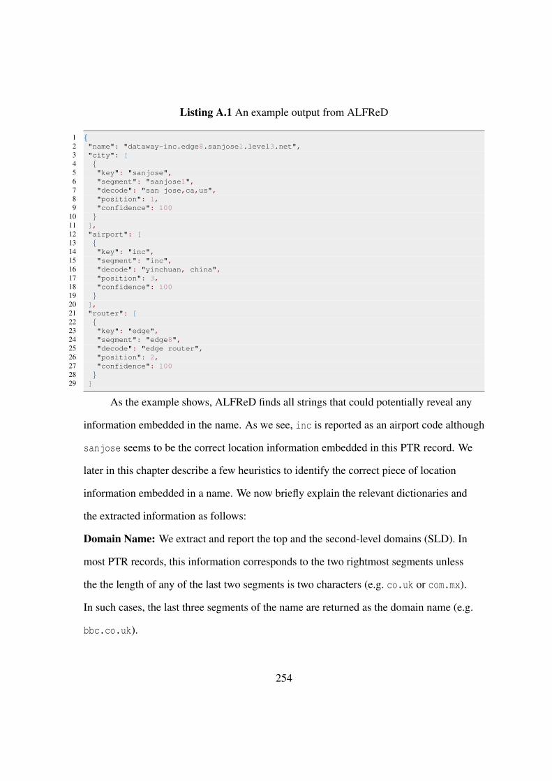
Listing A.1 An example output from ALFReD
1 {2 "name": "dataway-inc.edge8.sanjose1.level3.net",3 "city": [4 {5 "key": "sanjose",6 "segment": "sanjose1",7 "decode": "san jose,ca,us",8 "position": 1,9 "confidence": 100
10 }11 ],12 "airport": [13 {14 "key": "inc",15 "segment": "inc",16 "decode": "yinchuan, china",17 "position": 3,18 "confidence": 10019 }20 ],21 "router": [22 {23 "key": "edge",24 "segment": "edge8",25 "decode": "edge router",26 "position": 2,27 "confidence": 10028 }29 ]
As the example shows, ALFReD finds all strings that could potentially reveal any
information embedded in the name. As we see, inc is reported as an airport code although
sanjose seems to be the correct location information embedded in this PTR record. We
later in this chapter describe a few heuristics to identify the correct piece of location
information embedded in a name. We now briefly explain the relevant dictionaries and
the extracted information as follows:
Domain Name: We extract and report the top and the second-level domains (SLD). In
most PTR records, this information corresponds to the two rightmost segments unless
the the length of any of the last two segments is two characters (e.g. co.uk or com.mx).
In such cases, the last three segments of the name are returned as the domain name (e.g.
bbc.co.uk).
254

Interface Technology: We consider commonly used interface technology conventions
from Cisco [73], Juniper [147] and Huawei [134] to populate a dictionary of commonly
used terms that refer to port technologies. We also consider guidelines provided
by NANOG [246] to improve this dictionary. Overall this dictionary includes 150
keywords. Few interface codes overlap with the geo location dictionaries, for instance,
wan is conventionally used for “Wide Area Networks” and is also the airport code for
“Waverney” airport in Australia, so extra care is necessary in inferring the correct
information from these keywords. As a common strategy, ALFReD reports all possible
hints and delegates any speculations to the user.
Router: ALFReD also reports network related keywords (e.g. “wireless”, “host”, “edge”)
which hint at the router’s attribute [246]. We build a dictionary of these keywords
totalling 58 entries. While this dictionary started as one that was built solely using domain
knowledge and a manual inspection of names, it was later expanded using techniques
explained later in the chapter.
Location Information: We have used a few separate dictionaries for extracting location
information (geo hints) from a PTR record. Our first dictionary is 3-letter airport codes.
We collected airport codes from airportcodes.org [1] which includes more than 3.5K
airport codes. Second, we use CLLI codes. A CLLI code (Common Language Location
Identifier) is used within the North American telecommunications industry to specify the
location of a telecommunication equipment. We obtained a total of 22K 6-letter CLLI
codes from telcodata.us [6]. Note that each city does not have a unique CLLI code, for
instance ‘STTLWA’, ‘STTMWA’ and ‘STTNWA’ are all valid CLLI codes for Seattle,
WA. We also observed the usage of many 4-letter CLLI codes. Hence, we added 11K
4-letter CLLI codes to this dictionary as well. Third, we check each segment against
255
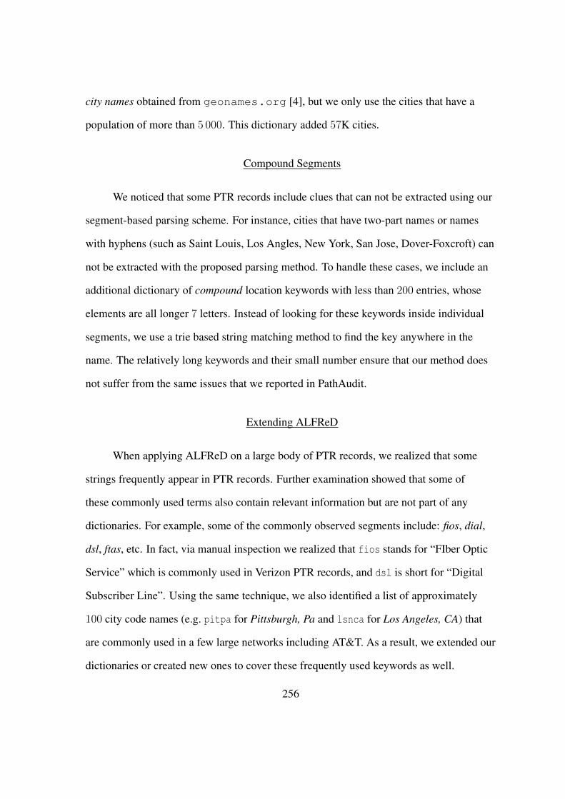
city names obtained from geonames.org [4], but we only use the cities that have a
population of more than 5 000. This dictionary added 57K cities.
Compound Segments
We noticed that some PTR records include clues that can not be extracted using our
segment-based parsing scheme. For instance, cities that have two-part names or names
with hyphens (such as Saint Louis, Los Angles, New York, San Jose, Dover-Foxcroft) can
not be extracted with the proposed parsing method. To handle these cases, we include an
additional dictionary of compound location keywords with less than 200 entries, whose
elements are all longer 7 letters. Instead of looking for these keywords inside individual
segments, we use a trie based string matching method to find the key anywhere in the
name. The relatively long keywords and their small number ensure that our method does
not suffer from the same issues that we reported in PathAudit.
Extending ALFReD
When applying ALFReD on a large body of PTR records, we realized that some
strings frequently appear in PTR records. Further examination showed that some of
these commonly used terms also contain relevant information but are not part of any
dictionaries. For example, some of the commonly observed segments include: fios, dial,
dsl, ftas, etc. In fact, via manual inspection we realized that fios stands for “FIber Optic
Service” which is commonly used in Verizon PTR records, and dsl is short for “Digital
Subscriber Line”. Using the same technique, we also identified a list of approximately
100 city code names (e.g. pitpa for Pittsburgh, Pa and lsnca for Los Angeles, CA) that
are commonly used in a few large networks including AT&T. As a result, we extended our
dictionaries or created new ones to cover these frequently used keywords as well.
256

Heuristic for Resolving Conflicting Information
As shown before in Listing A.1, different segments of a name may hint at
conflicting information. This issue is more problematic in the case of conflicting
location information. For instance, due to the abundance of airport codes, a segment
inside a name may match a code that does not reveal the location in reality (e.g.
although inc is an airport code, it does not seem to reveal the correct location in
dataway-inc.edge8.sanjose1.level3.net). We use three simple heuristics to identify
the location information with the highest likelihood of correctness.
Overlapping Dictionaries: A key may exist in two different dictionaries. For instance,
bbr could both refer to a backbone router or Baillif Airport. When a segment matches a
key in two different dictionaries, we assign a lower confidence to it compared to the case
when the key is only in one dictionary. The correct location code is most likely among the
the keys with the highest confidence.
Key Length: If two location codes are found in a name, we first compare their length
then and select the longer one. The rationale is that the likelihood of two strings randomly
matching each other is inversely proportional to the strings’ length.
Segment Position: In addition to the key itself, ALFReD also returns the position of
the segment where the keyword is identified. Examining a large body of PTR records
and observing naming patterns and conventions followed by operators [246, 241], we
observed that keys that appear later in a PTR record likely reveal the location information.
This heuristic is used as the last tie breaker to identify the correct location information.
ALFReD in Action
In this section we analyze the results from parsing a large set of PTR records using
ALFReD. This analysis not only shows the functionality of ALFReD as an tool to extract
257

information from PTR records, but also allows us to see the frequency and the different
type of information that is coded in PTR records by different administrators. We also use
PathAudit [61, 62] and DRoP [135] to compare ALFReD with its rivals.
Mapping ASes Using ALFReD
In our first case study, we use ALFReD to reveal information in the PTR records
assigned by one AS. Since our goal is to analyze and compare PTR records assigned
by different ASes, we use the methodology similar to the one proposed by Ferguson
et al. [105] to maximize the number of names recovered for each AS. However, we try
to minimize the effort in searching for PTR records used by an AS as we explain the
following: Instead of sweeping the entire IP space assigned to our target AS, we only
focus on /24 prefixes that the AS uses for assigning IPs to network devises. To find these
prefixes, we use CAIDA’s ARK project dataset [51]. The dataset is collected as the result
of CAIDA’s large-scale traceroute-based measurements. We first identify all IPs observed
in their measurements during September of 2015. We then map each IP to an AS number
using Team Cymru’s whois tool [250]. We finally include all /24 prefixes that contain
the IPs that belong to our target ASes. We perform reverse DNS look up using dig
command [140, 2] to scan all IPs in the selected prefixes of our target ASes.
We focus on four large ASes, namely AT&T, Level3, Cogent, and Verizon. We
identified 157, 682, 404, and 35 503 prefixes in these networks respectively. Using the
described dig-based reverse DNS look up method, we find 40K, 174K, 103K, and 9M
PTR records in these prefixes respectively. Interestingly the domain name of these IPs
does not always correspond with the PTR assigned to the same AS. Figure A.63 shows
the domain names of IPs in three of these AS’s IP space. In order to study the AS specific
conventions and type of informations embedded in each AS we only focus on the PTR
258
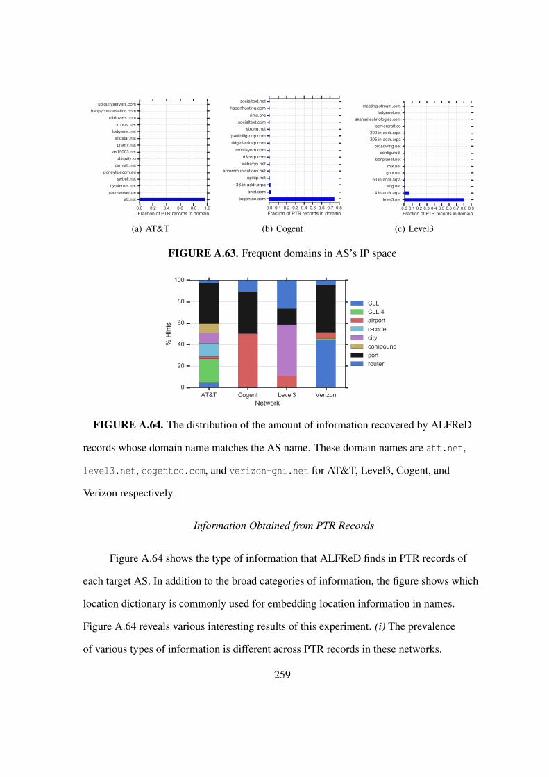
0.0 0.2 0.4 0.6 0.8 1.0Fraction of PTR records in domain
att.netyour-server.denyinternet.net
swbell.netponeytelecom.eu
zermatt.netubiquity.io
as15003.netprserv.net
wildstar.netlodgenet.net
irchost.netunixlovers.com
happyconversation.comubiquityservers.com
(a) AT&T
0.0 0.1 0.2 0.3 0.4 0.5 0.6 0.7 0.8Fraction of PTR records in domain
cogentco.comanet.com
38.in-addr.arpaepikip.net
arcommunications.netwebaxys.netd3corp.com
morrisyorn.comridgefieldcap.comparkhillgroup.com
strong.netsocialtext.com
rims.orghagenhosting.com
socialtext.net
(b) Cogent
0.0 0.1 0.2 0.3 0.4 0.5 0.6 0.7 0.8 0.9Fraction of PTR records in domain
level3.net4.in-addr.arpa
wcg.net63.in-addr.arpa
gblx.netmik.net
bbnplanet.netconfigured.
broadwing.net205.in-addr.arpa209.in-addr.arpa
servercraft.coakamaitechnologies.com
lodgenet.netmeeting-stream.com
(c) Level3
FIGURE A.63. Frequent domains in AS’s IP space
AT&T Cogent Level3 VerizonNetwork
0
20
40
60
80
100
% H
ints
CLLICLLI4airportc-codecitycompoundportrouter
FIGURE A.64. The distribution of the amount of information recovered by ALFReD
records whose domain name matches the AS name. These domain names are att.net,
level3.net, cogentco.com, and verizon-gni.net for AT&T, Level3, Cogent, and
Verizon respectively.
Information Obtained from PTR Records
Figure A.64 shows the type of information that ALFReD finds in PTR records of
each target AS. In addition to the broad categories of information, the figure shows which
location dictionary is commonly used for embedding location information in names.
Figure A.64 reveals various interesting results of this experiment. (i) The prevalence
of various types of information is different across PTR records in these networks.
259

(ii) Location information extracted from AT&T’s PTR records come from various
dictionaries, but the other networks seem to use conventions that strictly use certain types
of keywords. (iii) A large amount of router role information can be inferred from names
used in Level3. This fraction of router role information extracted from names in other
networks is much less. (iv) The yield of different location dictionaries is AS dependent.
While the usage of CLLI codes is frequent in Verizon, Cogent uses airport codes and
Level3 prefers to use city names.
Mapping Footprint of ASes with ALFReD
We use the location information inferred from the PTR records of each network to
find its geographical coverage. For comparison, we also use MaxMind IP geolocation
dataset [184] and find the geo footprint of the target ASes using this dataset as well.
Figure A.65 presents comparative views of these inferred geo-footprints using the two
geolocation tools. As all the figures show, MaxMind only geolocates the IPs to the United
States and does not provide a finer resolution for geolocation. However, ALFReD is
able to geolocate the reverse DNS names of these IPs to specific cities in the United
States. The plots reveal that all the target ASes have mostly similar coverage with large
deployments along the coasts and also considerable IPs in the Midwest.
ALFReD vs. its Rivals
In this section we use ALFReD to infer the information from a pool of PTR records
from various ASes. To this end, we use the PTR records provided by CAIDA’s Ark
project [8]. Due to the large scale of the measurement campaign and scheduling scheme
of this project, this dataset contains names from all major ASes. We use this dataset to
compare the location information extracted by ALFReD to those of DRoP and PathAudit.
260
ALFReD
MaxMind
(a) AT&T
ALFReD
MaxMind
(b) Cogent
ALFReD
MaxMind
(c) Level3
ALFReD
MaxMind
(d) Verizon
FIGURE A.65. Comparison of IP-geolocation using MaxMind (bottom) and DNS-geolocataion using ALFReD (top) for four target networks
Figure A.67 shows the coverage of these three parsing tools using a Venn diagram. While
ALFReD is capable of extracting location information from 228K (22%) of the 1M PTR
records obtained from CAIDA, this number is 112K (11%) and 5K (5%) for DRoP and
PathAudit, respectively. These results clearly show that ALFReD is more capable of
extracting location information from PTR records assigned by various ASes.
261

8K107K7K
487K
69K 174K28K
DRoPPathAudit
ALFReD
FIGURE A.66. Comparison ofthe number of PTR records that areparsed by each tool
31K
24K1K
135K
72K 13K9K
DRoPPathAudit
ALFReD
FIGURE A.67. Comparison of thenumber of PTR records that pack alocation information according toeach tool
We also examine the records that are parsed by DRoP and PathAudit but not
ALFReD. Specifically, we check the geo-hints extracted by each tool. If these hints
are correctly extracted by other tools, we can add them to ALFReD’s dictionaries as
well. Figure A.68 provides the number of times each geo-hint is extracted from all PTR
records in this dataset. We make the following observations from these plots: (i) Many
geo-hints extracted by DRoP do not seem to be keywords that are easily recognizable.
Our manual examination of many of these character strings did not reveal any indication
that the string could refer to a location. In the case of PathAudit, some of the extracted
strings can be recognized (e.g. pennsylvania). Many of these strings are state names,
and are ignored by ALFReD as a result of our city-level geolocation focus. Another issue
with respect to PathAudit results is its parsing mechanism, which looks for dictionary
keys anywhere in the PTR record. For instance PathAudit infers reno as a geo-hint from
renovation.yourespressob1.com, tge1-7-1-1.grenoh1-rtr800.div.neo.rr.com
and laco01-c1.core02.mtl-1250.fibrenoire.ca which are obviously incorrect. (ii)
Comparing the distribution of geo-hints extracted exclusively by ALFReD and those that
262
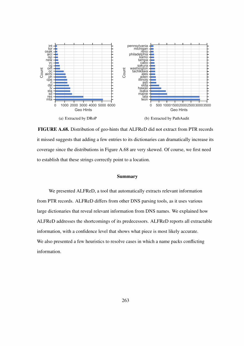
0 1000 2000 3000 4000 5000 6000Geo Hints
mtaressdsta
lvdsl
ricpeph
aichioc
omcgvc
newispaici
osaktorint
Cou
nt
(a) Extracted by DRoP
0 500 100015002000250030003500Geo Hints
leonlala
maineisaka
hawaiieldaasti
illinoisadenales
tachikawawashington
sakuracabo
tampakamo
philadelphiareno
michiganpennsylvania
Cou
nt(b) Extracted by PathAudit
FIGURE A.68. Distribution of geo-hints that ALFReD did not extract from PTR records
it missed suggests that adding a few entries to its dictionaries can dramatically increase its
coverage since the distributions in Figure A.68 are very skewed. Of course, we first need
to establish that these strings correctly point to a location.
Summary
We presented ALFReD, a tool that automatically extracts relevant information
from PTR records. ALFReD differs from other DNS parsing tools, as it uses various
large dictionaries that reveal relevant information from DNS names. We explained how
ALFReD addresses the shortcomings of its predecessors. ALFReD reports all extractable
information, with a confidence level that shows what piece is most likely accurate.
We also presented a few heuristics to resolve cases in which a name packs conflicting
information.
263

REFERENCES CITED
[1] Airport Codes. https://www.airportcodes.org. Accessed: 2014-09-05.
[2] Domain Names - Implementation and Specification.https://www.ietf.org/rfc/rfc1035.txt. Accessed: 2014-09-16.
[3] Equinix Q1 2016 Earnings Conference Call.http://phx.corporate-ir.net/External.File?item=UGFyZW50SUQ9MzM2OTc1fENoaWxkSUQ9LTF8VHlwZT0z&t=1&cb=635979891794307751.
[4] GeoNames. https://www.geonames.org. Accessed: 2014-09-05.
[5] Sankey diagram. https://en.wikipedia.org/wiki/Sankey_diagram.
[6] Telcodata.us telecommunications database. https://www.telcodata.us.Accessed: 2014-09-05.
[7] Telx Cross Connects. http://www.telx.com/interconnection/.
[8] The CAIDA UCSD IPv4 Routed /24 DNS Names Dataset. http://www.caida.org/data/active/ipv4_dnsnames_dataset.xml.Accessed: 2014-09-09.
[9] RIPE RIS. https://www.ripe.net/data-tools/stats/ris/routing-information-service, 2011.
[10] A. Dhamdhere and C. Dovrolis. Twelve years in the evolution of the Internetecosystem. IEEE/ACM Transactions on Networking (ToN), 19(5), 2011.
[11] L. A. Adamic and N. Glance. The political blogosphere and the 2004 us election:divided they blog. In Proc. of the workshop on Link discovery. ACM, 2005.
[12] Advanced Network Technology Center. University of Oregon Route Views Project.http://www.routeviews.org, 2013.
[13] B. Ager, N. Chatzis, A. Feldmann, N. Sarrar, S. Uhlig, and W. Willinger. Anatomy ofa large european IXP. In Proc. of SIGCOMM. ACM, 2012.
[14] R. Agrawal, B. Golshan, and E. Papalexakis. Homogeneity in web search results:Diagnosis and mitigation. Technical Report TR-2015-007, Data InsightsLaboratories, San Jose, California, June 2015.
[15] R. Agrawal, B. Golshan, and E. Papalexakis. Overlap between google and bing websearch results!: Twitter to the rescue? In Proc. of COSN. ACM, 2015.
264

[16] Y. Y. Ahn, S. Han, H. Kwak, S. Moon, and H. Jeong. Analysis of TopologicalCharacteristics of Huge Online Social Networking Services. In Proc. of WWW.ACM, 2007.
[17] Akamai. EdgeScape Service Description. http://uk.akamai.com/dl/brochures/edgescape_service_description.pdf, March 2002.
[18] R. Albert and A.-L. Barabasi. Statistical mechanics of complex networks. Reviews ofModern Physics, 74(1), 2002.
[19] R. Albert, H. Jeong, and A.-L. Barabasi. Error and attack tolerance of complexnetworks. Nature, 406(6794), 2000.
[20] A. Alvarez-Socorro, G. Herrera-Almarza, and L. Gonzalez-Dıaz. Eigencentralitybased on dissimilarity measures reveals central nodes in complex networks.Scientific reports, 5, 2015.
[21] L. A. N. Amaral, A. Scala, M. Barthelemy, and H. E. Stanley. Classes of small-worldnetworks. Proc. of NAS, 97(21), 2000.
[22] R. Andersen, F. Chung, and K. Lang. Local graph partitioning using pagerankvectors. In Proc. of Foundations of Computer Science (FOCS). IEEE, 2006.
[23] B. Augustin, X. Cuvellier, B. Orgogozo, F. Viger, T. Friedman, M. Latapy,C. Magnien, and R. Teixeira. Avoiding Traceroute Anomalies with ParisTraceroute. In Proc. of IMC. ACM SIGCOMM, 2006.
[24] B. Augustin, B. Krishnamurthy, and W. Willinger. IXPs: Mapped? In Proc. of IMC.ACM, 2009.
[25] C. Avin, Z. Lotker, and Y.-A. Pignolet. On the elite of social networks. PersonalCommunication, 2012.
[26] C. Avin, Z. Lotker, Y.-A. Pignolet, and I. Turkel. From caesar to twitter: an axiomaticapproach to elites of social networks. arXiv preprint arXiv:1111.3374, 2011.
[27] K. Avrachenkov, N. Litvak, L. O. Prokhorenkova, and E. Suyargulova. Quickdetection of high-degree entities in large directed networks. In Proc. of ICDM.IEEE, 2014.
[28] B. Eriksson, P. Barford and J. Sommers and R. Nowak. Inferring UnseenComponents of the Internet Core. Journal on Selected Areas in Communications,IEEE, 29(9), 2011.
[29] L. Backstrom, P. Boldi, M. Rosa, J. Ugander, and S. Vigna. Four Degrees ofSeparation. CoRR, abs/1111.4570, 2011.
265

[30] E. Bakshy, J. M. Hofman, W. A. Mason, and D. J. Watts. Everyone’s an influencer:quantifying influence on twitter. In Proc. of WSDM. ACM, 2011.
[31] E. Bakshy, J. M. Hofman, W. A. Mason, and D. J. Watts. Identifying influencers ontwitter. In Proc. of WSDM. ACM, 2011.
[32] Balakrishnan Chandrasekaran and Georgios Smaragdakis and Arthur Berger andMatthew Luckie and Keung-Chi Ng. A Server-to-Server View of the Internet. InProc. of CoNEXT. ACM, 2015.
[33] P. Barford, A. Bestavros, J. Byers, and M. Crovella. On the marginal utility ofnetwork topology measurements. In Proc. of IMC. ACM SIGCOMM, 2001.
[34] D. Barnes and B. Sakandar. Cisco LAN switching fundamentals. Cisco Press, 2004.
[35] T. Barnett. 2015 cisco vni complete forecast update: Key trends include mobility,m2m and multimedia content. http://blogs.cisco.com/sp/2015-cisco-vni-complete-forecast-update-key-trends-include-mobility-m2m-and-multimedia-content, 2015.
[36] M. Bastian, S. Heymann, M. Jacomy, et al. Gephi: An Open Source Software forExploring and Manipulating Networks. AAAI, 2009.
[37] A. Bender, R. Sherwood, and N. Spring. Fixing ally’s growing pains with velocitymodeling. In Proc. of IMC. ACM SIGCOMM, 2008.
[38] F. Benevenuto, T. Rodrigues, M. Cha, and V. Almeida. Characterizing user behaviorin online social networks. In Proc. of IMC. ACM SIGCOMM, 2009.
[39] R. Beverly, A. Berger, and G. G. Xie. Primitives for active Internet topologymapping: Toward high-frequency characterization. In Proc. of IMC. ACMSIGCOMM, 2010.
[40] V. D. Blondel, J.-L. Guillaume, R. Lambiotte, and E. Lefebvre. Fast unfolding ofcommunities in large networks. Journal of Statistical Mechanics: Theory andExperiment, 2008(10), 2008.
[41] B. Bollobas. Modern graph theory, volume 184. Springer Science & Business Media,2013.
[42] V. Bolotaeva and T. Cata. Marketing opportunities with social networks. Journal ofInternet Social Networking and Virtual Communities, 2010, 2010.
[43] S. P. Borgatti. Identifying sets of key players in a social network. Computational &Mathematical Organization Theory, 12(1), 2006.
[44] A. Boutet, A. Kermarrec, E. Le Merrer, and A. Van Kempen. On the impact of usersavailability in osns. In ACM SNS, 2012.
266

[45] C. M. Bowman, P. B. Danzig, U. Manber, and M. F. Schwartz. Scalable Internetresource discovery: Research problems and approaches. Communications of theACM-Association for Computing Machinery-CACM, 37(8), 1994.
[46] S. Brin and L. Page. The anatomy of a large-scale hypertextual web search engine. InProc. of WWW), 1998.
[47] S. Brin and L. Page. Reprint of: The anatomy of a large-scale hypertextual websearch engine. Computer Networks, 56(18), 2012.
[48] P. Brodka, S. Saganowski, and P. Kazienko. Group evolution discovery in socialnetworks. In Advances in Social Networks Analysis and Mining (ASONAM). IEEE,2011.
[49] R. Bush, O. Maennel, M. Roughan, and S. Uhlig. Internet optometry: assessing thebroken glasses in Internet reachability. In Proc. of IMC. ACM SIGCOMM, 2009.
[50] X. Cai, J. Heidemann, B. Krishnamurthy, and W. Willinger. Towards anAS-to-organization Map. In Proc. of IMC. ACM SIGCOMM, 2010.
[51] CAIDA. Archipelago (Ark) Measurement Infrastructure.http://www.caida.org/projects/ark/.
[52] CAIDA. AS Rank: AS Ranking. http://as-rank.caida.org/.
[53] CAIDA. AS Relationships.http://www.caida.org/data/as-relationships/.
[54] CAIDA. Skitter.http://www.caida.org/tools/measurement/skitter/.
[55] G. Caldarelli. Scale-free networks: complex webs in nature and technology. OUPCatalogue, 2007.
[56] R. W. Callon. Use of OSI IS-IS for routing in TCP/IP and dual environments. rfc1195: see online http://tools.ietf.org/html/rfc1195, 1990.
[57] R. Campigotto, J.-L. Guillaume, and M. Seifi. The power of consensus: randomgraphs have no communities. In Proc. of ASONAM. ACM, 2013.
[58] Q. Cao, M. Sirivianos, X. Yang, and T. Pregueiro. Aiding the Detection of FakeAccounts in Large Scale Social Online Services. In Proc. of NSDI, 2012.
[59] M. Cha, H. Haddadi, F. Benevenuto, and P. K. Gummadi. Measuring user influence intwitter: The million follower fallacy. AAAI, 2010.
267

[60] M. Cha, A. Mislove, and K. P. Gummadi. A measurement-driven analysis ofinformation propagation in the flickr social network. In Proc. of WWW. ACM,2009.
[61] J. Chabarek. PathAudit.https://github.com/jc-wail/WAIL/tree/master/PathAudit.
[62] J. Chabarek and P. Barford. What’s in a name?: decoding router interface names. InProc. of IMC. ACM SIGCOMM, 2013.
[63] H. Chang, S. Jamin, and W. Willinger. Inferring AS-level Internet topology fromrouter-level path traces. In ITCom. International Society for Optics and Photonics,2001.
[64] H. Chang, S. Jamin, and W. Willinger. Internet connectivity at the AS-level: anoptimization-driven modeling approach. In Proc. of the MoMeTools workshop.ACM SIGCOMM, 2003.
[65] H. Chang, S. Jamin, and W. Willinger. To peer or not to peer: Modeling the evolutionof the Internet’s AS-level topology. Ann Arbor, 1001, 2006.
[66] N. Chatzis, G. Smaragdakis, J. Bottger, T. Krenc, and A. Feldmann. On the benefitsof using a large IXP as an Internet vantage point. In Proc. of IMC. ACMSIGCOMM, 2013.
[67] N. Chatzis, G. Smaragdakis, A. Feldmann, and W. Willinger. There is more to IXPsthan meets the eye. ACM SIGCOMM Computer Communication Review, 43(5),2013.
[68] K. Chen, D. R. Choffnes, R. Potharaju, Y. Chen, F. E. Bustamante, D. Pei, andY. Zhao. Where the sidewalk ends: Extending the Internet AS graph usingtraceroutes from P2P users. In Proc. of CoNEXT. ACM, 2009.
[69] W. Chen, Y. Huang, B. F. Ribeiro, K. Suh, H. Zhang, E. d. S. e Silva, J. Kurose, andD. Towsley. Exploiting the IPID field to infer network path and end-systemcharacteristics. In Proc. of the PAM. Springer, 2005.
[70] D. Choi, J. Han, T. Chung, Y.-Y. Ahn, B.-G. Chun, and T. T. Kwon. Characterizingconversation patterns in reddit: From the perspectives of content properties and userparticipation behaviors. In Proc. of COSN. ACM, 2015.
[71] B. Chun, D. Culler, T. Roscoe, A. Bavier, L. Peterson, M. Wawrzoniak, andM. Bowman. Planetlab: an overlay testbed for broad-coverage services. ACMSIGCOMM Computer Communication Review, 2003.
[72] F. R. Chung. Spectral Graph Theory, volume 92. American Mathematical Soc., 1997.
268

[73] Cisco Systems. Configuring Router Interfaces.http://www.cisco.com/c/en/us/td/docs/security/security_management/cisco_security_manager/security_manager/4-1/user/guide/CSMUserGuide_wrapper/rtintf.pdf.
[74] A. Clauset, C. R. Shalizi, and M. E. Newman. Power-law distributions in empiricaldata. SIAM review, 51(4), 2009.
[75] P. Cogan, M. Andrews, M. Bradonjic, W. S. Kennedy, A. Sala, and G. Tucci.Reconstruction and analysis of twitter conversation graphs. In Proc. of Workshop onHotSocial. ACM, 2012.
[76] CoreSite. CoreSite Cross Connects.http://www.coresite.com/solutions/interconnection/cross-connects. Accessed: 2016-06-01.
[77] CoreSite. CoreSite: Investor Presentation, June 2016.http://phx.corporate-ir.net/External.File?item=UGFyZW50SUQ9NjM2NTEwfENoaWxkSUQ9MzQwOTY3fFR5cGU9MQ==&t=1.
[78] CoreSite. CoreSite SEC Filings 02/12/2016.http://www.coresite.com/investors/financial-reports/sec-filings.
[79] CoreSite. THE CORESITE OPEN CLOUD EXCHANGE - One Connection.Countless Cloud Options.http://www.coresite.com/solutions/cloud-services/open-cloud-exchange.
[80] W. de Donato, P. Marchetta, and A. Pescape. A hands-on look at active probing usingthe IP prespecified timestamp option. In Proc. of PAM. Springer, 2012.
[81] Q. Deng and Y. Dai. How your friends influence you: Quantifying pairwiseinfluences on twitter. In Prof. of the CSC. IEEE, 2012.
[82] A. Dhamdhere and C. Dovrolis. Ten years in the evolution of the Internet ecosystem.In Proc. of IMC. ACM SIGCOMM, 2008.
[83] I. S. Dhillon, Y. Guan, and B. Kulis. Kernel k-means: Spectral Clustering andNormalized Cuts. In Proc. of SIGKDD. ACM, 2004.
[84] I. S. Dhillon, Y. Guan, and B. Kulis. Weighted graph cuts without eigenvectors amultilevel approach. IEEE Transactions on Pattern Analysis and MachineIntelligence (TPAMI), 29(11), 2007.
269

[85] G. Di Battista, M. Patrignani, and M. Pizzonia. Computing the types of therelationships between autonomous systems. In Proc. of the INFOCOM, volume 1.IEEE, 2003.
[86] R. Diestel. Graph theory {graduate texts in mathematics; 173}. Springer-VerlagBerlin and Heidelberg GmbH & amp, 2000.
[87] X. A. Dimitropoulos, D. V. Krioukov, and G. F. Riley. Revisiting Internet AS-leveltopology discovery. In Proc. of PAM. Springer, 2005.
[88] H. N. Djidjev. A Scalable Multilevel Algorithm for Graph Clustering and CommunityStructure Detection. In Algorithms and Models for the Web-Graph. Springer, 2008.
[89] G. W. Domhoff. Who rules America?: power and politics, and social change.McGraw-Hill Humanities, Social Sciences & World Languages, 2006.
[90] P. Domingos and M. Richardson. Mining the network value of customers. In Proc. ofSIGKDD. ACM, 2001.
[91] B. Donnet and T. Friedman. Internet topology discovery: a survey. CommunicationsSurveys & Tutorials, IEEE, 9(4), 2007.
[92] B. Donnet, M. Luckie, P. Merindol, and J.-J. Pansiot. Revealing MPLS tunnelsobscured from traceroute. ACM SIGCOMM Computer Communication Review,42(2), 2012.
[93] B. Donnet, P. Raoult, T. Friedman, and M. Crovella. Deployment of an algorithm forlarge-scale topology discovery. Journal on Selected Areas in Communications,IEEE, 24(12), 2006.
[94] R. Durairajan, S. Ghosh, X. Tang, P. Barford, and B. Eriksson. Internet Atlas: aGeographic Database of the Internet. In Proc. of the Workshop HotPlanet. ACM,2013.
[95] R. Durairajan, J. Sommers, and P. Barford. Layer 1-Informed Internet TopologyMeasurement. In Proc. of IMC, 2014.
[96] R. Durairajan, J. Sommers, W. Willinger, and P. Barford. InterTubes: A Study of theUS Long-haul Fiber-optic Infrastructure. In Proc. of the SIGCOMM, 2015.
[97] D. Easley and J. Kleinberg. Networks, crowds, and markets: Reasoning about ahighly connected world. Cambridge University Press, 2010.
[98] H. Electric. Hurricane Electric BGP Toolkit. http://bgp.he.net/.
[99] Equninix. Equinix Reports Fourth Quarter and Year-End 2015 Results.http://www.equinix.com/company/news-and-events/press-releases/equinix-reports-fourth-quarter-2014-results/.
270

[100] Equninix. Historical Quarterly and Year-End Results. http://investor.equinix.com/phoenix.zhtml?c=122662&p=quarterlyearnings.
[101] B. Eriksson, P. Barford, J. Sommers, and R. Nowak. DomainImpute: Inferringunseen components in the Internet. In Proc. of INFOCOM. IEEE, 2011.
[102] M. Faloutsos, P. Faloutsos, and C. Faloutsos. On power-law relationships of theInternet topology. 29(4), 1999.
[103] N. Feamster. Revealing Utilization at Internet Interconnection Points. Available atSSRN 2756888, 2016.
[104] D. Feldman and Y. Shavitt. Automatic large scale generation of Internet pop levelmaps. In IEEE GLOBECOM 2008. IEEE, 2008.
[105] A. D. Ferguson, J. Place, and R. Fonseca. Growth analysis of a large ISP. In Proc.of IMC. ACM SIGCOMM, 2013.
[106] D. Fitzgerald. Equinix Inc., the Internet’s Biggest Landlord.http://www.wsj.com/articles/equinix-inc-the-internets-biggest-landlord-1414451918.
[107] S. Fortunato. Community detection in graphs. Physics Reports, 486(3), 2010.
[108] L. C. Freeman. A set of measures of centrality based on betweenness. Sociometry,1977.
[109] T. M. Fruchterman and E. M. Reingold. Graph drawing by force-directedplacement. Software: Practice and experience, 21(11), 1991.
[110] S. Gaito, M. Zignani, G. Rossi, A. Sala, X. Wang, H. Zheng, and B. Zhao. On thebursty evolution of online social networks. In Proc. of KDD HotSocial Workshop.ACM, 2012.
[111] J. Ganesh. Social network analysis reveals the alternative list of global power elite.http://www.datasciencecentral.com/profiles/blogs/the-alternative-list-of-global-power-elite,2015.
[112] L. Gao. On inferring autonomous system relationships in the Internet. IEEE/ACMTransactions on Networking (ToN), 9(6), 2001.
[113] D. Garcia, P. Mavrodiev, and F. Schweitzer. Social resilience in online communities:The autopsy of friendster. In Proc. of COSN. ACM, 2013.
[114] S. Garg, T. Gupta, N. Carlsson, and A. Mahanti. Evolution of an online socialaggregation network: an empirical study. In Proc. of IMC. ACM SIGCOMM, 2009.
271

[115] V. Giotsas, G. Smaragdakis, B. Huffaker, M. Luckie, and k. claffy. Mapping PeeringInterconnections to a Facility. In Proc. of CoNEXT. ACM, Dec 2015.
[116] V. Giotsas, S. Zhou, M. Luckie, et al. Inferring Multilateral Peering. In Proc. ofCoNEXT. ACM, 2013.
[117] M. Gjoka, M. Kurant, C. Butts, and A. Markopoulou. Walking in facebook: A casestudy of unbiased sampling of osns. In IEEE INFOCOM, 2010.
[118] R. Gonzalez, R. Cuevas, R. Motamedi, R. Rejaie, and A. Cuevas. Google+ orgoogle-?. dissecting the evolution of the new osn in its first year. Technical reportavailable at:http://www.it.uc3m.es/˜rcuevas/techreports/g+TR2012.pdf,Universidad Carlos III de Madrid, 2012.
[119] R. Gonzalez, R. Cuevas, R. Motamedi, R. Rejaie, and A. Cuevas. Google+ orgoogle-?: dissecting the evolution of the new osn in its first year. In Proc. of WWW.International World Wide Web Conferences Steering Committee, 2013.
[120] R. Gonzalez, R. Cuevas, R. Motamedi, R. Rejaie, and A. Cuevas. Assessing theEvolution of Google+ in its First two Years. IEEE/ACM Transactions onNetworking (ToN), 2015.
[121] R. Govindan and A. Reddy. An analysis of Internet inter-domain topology and routestability. In Proc. of the INFOCOM, volume 2. IEEE, 1997.
[122] R. Govindan and H. Tangmunarunkit. Heuristics for Internet Map Discovery. InINFOCOM, volume 3. IEEE, 2000.
[123] Z. Govindarajulu. Rank correlation methods. Technometrics, 1992.
[124] B. Gueye, S. Uhlig, and S. Fdida. Investigating the imprecision of IP block-basedgeolocation. In Proc. of PAM. Springer, 2007.
[125] M. Gunes and K. Sarac. Resolving IP aliases in building traceroute-based Internetmaps. IEEE/ACM Transactions on Networking (ToN), 17(6), 2009.
[126] M. H. Gunes and K. Sarac. Analytical IP alias resolution. In Communications,2006. ICC’06. IEEE International Conference on, volume 1. IEEE, 2006.
[127] L. Gyarmati and T. Trinh. Measuring user behavior in online social networks.Network, IEEE, 2010.
[128] J. Han, D. Choi, A. Choi, J. Choi, T. Chung, T. T. Kwon, J.-Y. Rha, C.-N. Chuah,et al. Sharing topics in pinterest: Understanding content creation and diffusionbehaviors. In Proc. of COSN. ACM, 2015.
272

[129] S. Harenberg, G. Bello, L. Gjeltema, S. Ranshous, J. Harlalka, R. Seay,K. Padmanabhan, and N. Samatova. Community detection in large-scale networks:a survey and empirical evaluation. Wiley Interdisciplinary Reviews: Comput. Stat.,6(6), 2014.
[130] T. Hashimoto, Y. Sun, and T. Jaakkola. From random walks to distances onunweighted graphs. In Advances in Neural Information Processing Systems, 2015.
[131] G. Haviland. Designing High-Availability Campus Networks, 2000.
[132] J. Hawkinson and T. Bates. Guidelines for creation, selection, and registration of anAutonomous System (AS). RFC 1930 (Best Current Practice), Avaiable onlinehttp://www.ietf.org/rfc/rfc1930.txt, March 1996. Updated byRFC 6996.
[133] Y. He, G. Siganos, M. Faloutsos, and S. Krishnamurthy. Lord of the links: aframework for discovering missing links in the Internet topology. IEEE/ACMTransactions on Networking (ToN), 17(2), 2009.
[134] Huanetwork. The naming conventions of huawei ar routers.http://www.huanetwork.com/blog/the-naming-conventions-of-huawei-ar-routers/.
[135] B. Huffaker, M. Fomenkov, and k. claffy. DDec (BETA). http://ddec.caida.org/.
[136] B. Huffaker, M. Fomenkov, and k. claffy. DRoP:DNS-based Router Positioning.ACM SIGCOMM Computer Communication Review, 44(3), 2014.
[137] G. Huston. Interconnection, peering, and settlements. In Proc. of the INET,volume 9, 1999.
[138] Y. Hyun, A. Broido, and k. claffy. Traceroute and BGP AS Path Incongruities.Technical report, CAIDA, Mar 2003.
[139] Internet Routing Registry. Obtaining IRR Data.ftp://ftp.radb.net/radb/dbase, 2013.
[140] I. Internet Systems Consortium. Dig Manual Pages.https://ftp.isc.org/isc/bind9/cur/9.9/doc/arm/man.dig.html.
[141] IP2Location. IP2Location DB9, 2015. http://www.ip2location.com/,2015.
[142] T. Isdal, M. Piatek, A. Krishnamurthy, and T. Anderson. Leveraging BitTorrent forend host measurements. In Proc. of the PAM. Springer, 2007.
[143] V. Jacobson. Traceroute. see source code:ftp://ftp.ee.lbl.gov/traceroute.tar.gz.
273

[144] R. Jain, D.-M. Chiu, and W. R. Hawe. A quantitative measure of fairness anddiscrimination for resource allocation in shared computer system. Eastern ResearchLaboratory, Digital Equipment Corporation, 1984.
[145] J. Jiang, C. Wilson, X. Wang, P. Huang, W. Sha, Y. Dai, and B. Y. Zhao.Understanding Latent Interactions in Online Social Networks. In Proc. of IMC.ACM SIGCOMM, 2010.
[146] D. Joanes and C. Gill. Comparing measures of sample skewness and kurtosis.Journal of the Royal Statistical Society: Series D (The Statistician), 47(1), 1998.
[147] Juniper Systems, Inc. Interface naming overview.http://www.juniper.net/techpubs/en_US/junos12.3/topics/concept/interfaces-interface-naming-overview.html.
[148] S. Kairam, M. Brzozowski, D. Huffaker, and E. Chi. Talking in circles: Selectivesharing in google+. In Proc. of SIGCHI. ACM, 2012.
[149] R. Kannan, S. Vempala, and A. Vetta. On clusterings: Good, bad and spectral.Journal of the ACM (JACM), 51(3), 2004.
[150] G. Karypis and V. Kumar. METIS - Unstructured Graph Partitioning and SparseMatrix Ordering System, Version 2.0. 1995.
[151] G. Karypis and V. Kumar. A Fast and High Quality Multilevel Scheme forPartitioning Irregular Graphs. Journal on Scientific Computing, 20(1), 1998.
[152] V. Katsenelson. How I Bought the Internet - and You Can Too. http://www.institutionalinvestor.com/blogarticle/3310914/blog/how-i-bought-the-internetand-you-can-too.html#.VTl6IycVhBc.
[153] E. Katz-Bassett, H. V. Madhyastha, V. K. Adhikari, C. Scott, J. Sherry,P. Van Wesep, T. E. Anderson, and A. Krishnamurthy. Reverse traceroute. In NSDI,volume 10, 2010.
[154] D. Kemp, J. Kleinber, and E. Tardos. Maximizing the spread of influence in a socialnetwork. In Proc. of SIGKDD, 2003.
[155] T. Kernen. traceroute.org. http://www.traceroute.org.
[156] K. Keys. iffinder.http://www.caida.org/tools/measurement/iffinder/.
[157] K. Keys, Y. Hyun, M. Luckie, and K. Claffy. Internet-scale IPv4 alias resolutionwith MIDAR. IEEE/ACM Transactions on Networking (TON), 21(2), 2013.
[158] R. Kindermann, J. L. Snell, et al. Markov random fields and their applications,volume 1. American Mathematical Society Providence, RI, 1980.
274

[159] J. M. Kleinberg, R. Kumar, P. Raghavan, S. Rajagopalan, and A. S. Tomkins. TheWeb as a graph: measurements, models, and methods. In Computing andcombinatorics. Springer, 1999.
[160] S. Knight, H. X. Nguyen, N. Falkner, R. Bowden, and M. Roughan. The Internettopology zoo. Journal on Selected Areas in Communications, IEEE, 29(9), 2011.
[161] B. Krishnamurthy, W. Willinger, P. Gill, and M. Arlitt. A Socratic method forvalidation of measurement-based networking research. Computer Communications,34(1), 2011.
[162] R. Kumar, J. Novak, and A. Andtomkins. Structure and evolution of online socialnetworks. In Proc. of KDD. ACM, 2006.
[163] H. Kwak, C. Lee, H. Park, and S. Moon. What is Twitter, a Social Network or aNews Media? In Proc. of WWW. ACM, 2010.
[164] A. Lancichinetti and S. Fortunato. Community detection algorithms: a comparativeanalysis. Physical review E, 80(5), 2009.
[165] A. N. Langville and C. D. Meyer. Google’s PageRank and beyond: The science ofsearch engine rankings. Princeton University Press, 2011.
[166] S. Lattanzi and D. Sivakumar. Affiliation networks. In Proc. of STOC. ACM, 2009.
[167] W. E. Leland, M. S. Taqqu, W. Willinger, and D. V. Wilson. On the self-similarnature of Ethernet traffic. 23(4), 1993.
[168] J. Leskovec, J. Kleinberg, and C. Faloutsos. Graph evolution: Densification andshrinking diameters. ACM Transactions on Knowledge Discovery from Data(TKDD), 1(1), 2007.
[169] J. Leskovec, K. J. Lang, A. Dasgupta, and M. W. Mahoney. Community structure inlarge networks: Natural cluster sizes and the absence of large well-defined clusters.Internet Mathematics, 6(1), 2009.
[170] S. Lloyd. Least squares quantization in pcm. IEEE transactions on informationtheory, (2), 1982.
[171] A. Lodhi, A. Dhamdhere, and C. Dovrolis. Analysis of peering strategy adoption bytransit providers in the Internet. In Proc. of the INFOCOM Workshops, 2012.
[172] A. Lodhi, A. Dhamdhere, and C. Dovrolis. GENESIS: An agent-based model ofinterdomain network formation, traffic flow and economics. In Proc. of theINFOCOM. IEEE, 2012.
[173] L. Lovasz. Random Walks on Graphs: A Survey. Combinatorics, Paul erdos iseighty, 2(1), 1993.
275

[174] D. Lowd and A. Rooshenas. The libra toolkit for probabilistic models. Journal ofMachine Learning Research, 16, 2015.
[175] M. Luckie, A. Dhamdhere, D. Clark, B. Huffaker, et al. Challenges in InferringInternet Interdomain Congestion. In Proc. of IMC, 2014.
[176] M. Luckie, Y. Hyun, and B. Huffaker. Traceroute Probe Method and Forward IPPath Inference. In Proc. of IMC. ACM SIGCOMM, 2008.
[177] H. V. Madhyastha, T. Isdal, M. Piatek, C. Dixon, T. Anderson, A. Krishnamurthy,and A. Venkataramani. iPlane: An information plane for distributed services. InProc. of OSDI. USENIX, 2006.
[178] G. Magno, G. Comarela, D. Saez-Trumper, M. Cha, and V. Almeida. New Kid onthe Block: Exploring the Google+ Social Graph. In Proc. of IMC. ACMSIGCOMM, 2012.
[179] P. Mahadevan, D. Krioukov, M. Fomenkov, X. Dimitropoulos, A. Vahdat, et al. TheInternet AS-level topology: three data sources and one definitive metric. ACMSIGCOMM Computer Communication Review, 36(1), 2006.
[180] Z. M. Mao, R. Bush, T. G. Griffin, and M. Roughan. BGP Beacons. In Proc. ofIMC. ACM SIGCOMM, 2003.
[181] Z. M. Mao, L. Qiu, J. Wang, and Y. Zhang. On AS-level path inference. In ACMSIGMETRICS Performance Evaluation Review, volume 33. ACM, 2005.
[182] Z. M. Mao, J. Rexford, J. Wang, and R. H. Katz. Towards an accurate AS-leveltraceroute tool. In Proc. of the Conference on Applications, Technologies,Architectures, and Protocols for Computer Communications. ACM, 2003.
[183] P. Marchetta, V. Persico, E. Katz-Bassett, and A. Pescape. Dont trust traceroute(completely). In Proc. of CoNEXT Student workshop. ACM, 2013.
[184] MaxMind. Free World Cities Database.https://www.maxmind.com/en/free-world-cities-database.Accessed: 2015-12-01.
[185] MaxMind-LLC. GeoIP, 2016. http://www.maxmind.com, 2016.
[186] M. McPherson, L. Smith-Lovin, and J. M. Cook. Birds of a feather: Homophily insocial networks. Annual review of sociology, 2001.
[187] P. Merindol, V. Van den Schrieck, B. Donnet, O. Bonaventure, and J.-J. Pansiot.Quantifying ASes multiconnectivity using multicast information. In Proc. of IMC.AC SIGCOMMM, 2009.
276

[188] C. Metz. Interconnecting ISP networks. Internet Computing, IEEE, 5(2), 2001.
[189] D. L. Mills and H.-W. Braun. The NSFNET backbone network. 17(5), 1987.
[190] A. Mislove, H. S. Koppula, K. P. Gummadi, P. Druschel, and B. Bhattacharjee.Growth of the flickr social network. In Proc. of WOSN. ACM, 2008.
[191] A. Mislove, M. Marcon, K. P. Gummadi, P. Druschel, and B. Bhattacharjee.Measurement and Analysis of Online Social Networks. In Proc. of IMC. ACM,2007.
[192] G. Moore. The structure of a national elite network. American Sociological Review,1979.
[193] E. Mossel and S. Roch. On the submodularity of influence in social networks. InProc. of Symposium on Theory of Computing. ACM, 2007.
[194] R. Motamedi and R. a. Rejaie. ALFReD – Acquiring Location From Reverse DNS.atossa.cs.uoregon.edu:8080/alfred/, 2015.
[195] J. Moy. OSPF version 2. rfc 2328: see onlinehttp://tools.ietf.org/html/rfc2178, 1997.
[196] W. Muhlbauer, A. Feldmann, O. Maennel, M. Roughan, and S. Uhlig. Building anas-topology model that captures route diversity. ACM SIGCOMM ComputerCommunication Review, 36(4), 2006.
[197] A. Nazir, S. Raza, and C.-N. Chuah. Unveiling facebook: a measurement study ofsocial network based applications. In Proc. IMC. ACM, 2008.
[198] T. Nepusz, A. Petroczi, L. Negyessy, and F. Bazso. Fuzzy communities and theconcept of bridgeness in complex networks. Physical Review E, 77(1), 2008.
[199] M. Nerenberg, R. Motamedi, and R. Rejaie. Interactive Graph Coarsening byWalkAbout. Code available at:http://onrg.cs.uoregon.edu/WalkAbout, University of Oregon, 2014.
[200] M. E. Newman. The structure and function of complex networks. SIAM review,45(2), 2003.
[201] M. E. Newman. Modularity and community structure in networks. Proc. of NAS,103(23), 2006.
[202] R. Oliveira, D. Pei, W. Willinger, B. Zhang, and L. Zhang. The (in)completeness ofthe observed Internet AS-level structure. IEEE/ACM Transactions on Networking(ToN), 2010.
277

[203] R. Oliveira, W. Willinger, and B. Zhang. Quantifying the completeness of theobserved Internet AS-level structure. Technical report, UCLA, 080026, Sep 2008.
[204] R. V. Oliveira, D. Pei, W. Willinger, B. Zhang, and L. Zhang. In search of theelusive ground truth: the internet’s as-level connectivity structure. In ACMSIGMETRICS Performance Evaluation Review, volume 36. ACM, 2008.
[205] R. V. Oliveira, B. Zhang, and L. Zhang. Observing the evolution of Internet AStopology. ACM SIGCOMM Computer Communication Review, 37(4), 2007.
[206] T. Opsahl, V. Colizza, P. Panzarasa, and J. J. Ramasco. Prominence and control: theweighted rich-club effect. Physical review letters, 101(16), 2008.
[207] L. Page, S. Brin, R. Motwani, and T. Winograd. The PageRank citation ranking:bringing order to the Web. 1999.
[208] J.-J. Pansiot and D. Grad. On routes and multicast trees in the Internet. ACMSIGCOMM Computer Communication Review, 28(1), 1998.
[209] J.-J. Pansiot, P. Merindol, B. Donnet, and O. Bonaventure. Extracting intra-domaintopology from mrinfo probing. In Proc. of PAM. Springer, 2010.
[210] V. Paxson and S. Floyd. Wide area traffic: the failure of Poisson modeling.IEEE/ACM Transactions on Networking (ToN), 3(3), 1995.
[211] PeeringDB. Exchange Points List.https://www.peeringdb.com/private/participant_list.php,2013.
[212] I. Poese, S. Uhlig, M. A. Kaafar, B. Donnet, and B. Gueye. IP geolocationdatabases: unreliable? ACM SIGCOMM Computer Communication Review, 41(2),2011.
[213] P. Pons and M. Latapy. Computing communities in large networks using randomwalks. Journal of Graph Algorithms and Applications, 10(2), 2006.
[214] A. H. Rasti, N. Magharei, R. Rejaie, and W. Willinger. Eyeball ASes: fromgeography to connectivity. In Proc. of IMC. ACM SIGCOMM, 2010.
[215] A. H. Rasti, M. Torkjazi, R. Rejaie, N. Duffield, W. Willinger, and D. Stutzbach.Respondent-driven sampling for characterizing unstructured overlays. In Proc. ofthe INFOCOM. IEEE, 2009.
[216] G. Ravid and E. Currid-Halkett. The social structure of celebrity: an empiricalnetwork analysis of an elite population. Celebrity Studies, 4(2), 2013.
[217] R. Rejaie, M. Torkjazi, M. Valafar, and W. Willinger. Sizing Up Online SocialNetworks. IEEE Network, 2010.
278

[218] M. Richardson and P. Domingos. Mining knowledge-sharing sites for viralmarketing. In Proc. of SIGKDD. ACM, 2002.
[219] N. RIPE. Routing registry consistency check reports.http://www.ripe.net/projects/rrcc, 2009.
[220] Y. Rochat. Closeness centrality extended to unconnected graphs: The harmoniccentrality index. In ASNA, number EPFL-CONF-200525, 2009.
[221] E. M. Rogers. Diffusion of innovations. Simon and Schuster, 2010.
[222] M. Rosvall and C. Bergstrom. Maps of information flow reveal community structurein complex networks. In Proc. of the NAS. Citeseer, National Academy of Sciences,2007.
[223] M. Roughan, W. Willinger, O. Maennel, D. Perouli, and R. Bush. 10 Lessons from10 Years of Measuring and Modeling the Internets Autonomous Systems. SelectedAreas in Communications, 2011.
[224] M. A. Sanchez, J. S. Otto, Z. S. Bischof, D. R. Choffnes, F. E. Bustamante,B. Krishnamurthy, and W. Willinger. Dasu: Pushing experiments to the Internet’sedge. In Proc. of NSDI. USENIX, 2013.
[225] V. Satuluri and S. Parthasarathy. Scalable graph clustering using stochastic flows:applications to community discovery. In Proc. of KDD. ACM, 2009.
[226] S. Savage. Sting: A TCP-based Network Measurement Tool. In Proc. of USITS,volume 2. USENIX, 1999.
[227] D. Schioberg, F. Schneider, H. Schioberg, S. Schmid, S. Uhlig, and A. Feldmann.Tracing the birth of an osn: Social graph and profile analysis in google+. In ACMWebSci, 2012.
[228] F. Schneider, A. Feldmann, B. Krishnamurthy, and W. Willinger. Understandingonline social network usage from a network perspective. In Proc. of IMC. ACMSIGCOMM, 2009.
[229] M. Seifi, I. Junier, J.-B. Rouquier, S. Iskrov, and J.-L. Guillaume. Stable communitycores in complex networks. In Complex Networks. Springer, 2013.
[230] N. K. Sharma, S. Ghosh, F. Benevenuto, N. Ganguly, and K. Gummadi. Inferringwho-is-who in the twitter social network. ACM SIGCOMM ComputerCommunication Review, 42(4), 2012.
[231] Y. Shavitt and E. Shir. DIMES: Let the Internet measure itself. ACM SIGCOMMComputer Communication Review, 35(5), 2005.
279

[232] Y. Shavitt and U. Weinsberg. Quantifying the importance of vantage pointsdistribution in Internet topology measurements. In INFOCOM, IEEE. IEEE, 2009.
[233] Y. Shavitt and N. Zilberman. A structural approach for PoP geo-location. In Proc. ofthe INFOCOM. IEEE, 2010.
[234] Y. Shavitt and N. Zilberman. A geolocation databases study. Journal on SelectedAreas in Communications, IEEE, 29(10), 2011.
[235] R. Sherwood, A. Bender, and N. Spring. Discarte: a disjunctive Internetcartographer. 38(4), 2008.
[236] R. Sherwood and N. Spring. Touring the Internet in a TCP sidecar. In Proc. of IMC.ACM SIGCOMM, 2006.
[237] R. Siamwalla, R. Sharma, and S. Keshav. Discovering Internet Topology.Unpublished manuscript, 1998.
[238] A. Singla, B. Chandrasekaran, P. Godfrey, and B. Maggs. The internet at the speedof light. In Proc. of Hot Topics in Networks. ACM, 2014.
[239] S. Siwpersad, B. Gueye, and S. Uhlig. Assessing the geographic resolution ofexhaustive tabulation for geolocating internet hosts. In Proc. of PAM. Springer,2008.
[240] S. Sobolevsky, R. Campari, A. Belyi, and C. Ratti. General optimization techniquefor high-quality community detection in complex networks. Physical Review E,90(1), 2014.
[241] M. Solutions. A Proper Server Naming Scheme.https://www.mnxsolutions.com/devops/a-proper-server-naming-scheme.html. Accessed: 2014-09-05.
[242] J. Sommers, P. Barford, and B. Eriksson. On the prevalence and characteristics ofMPLS deployments in the open Internet. In Proc. of IMC. ACM SIGCOMM, 2011.
[243] N. Spring, M. Dontcheva, M. Rodrig, and D. Wetherall. How to resolve IP aliases.Technical report, Univ. Michigan, UW CSE Tech. Rep, 2004.
[244] N. Spring, R. Mahajan, and D. Wetherall. Measuring isp topologies with rocketfuel.ACM SIGCOMM Computer Communication Review, 32(4), 2002.
[245] N. T. Spring, D. Wetherall, and T. E. Anderson. Scriptroute: A Public InternetMeasurement Facility. In Proc. of USITS. USENIX, 2003.
[246] R. A. Steenbergen. A practical guide to (correctly) troubleshooting with traceroute.North American Network Operators Group, 2009.
280

[247] D. Strang and S. A. Soule. Diffusion in organizations and social movements: Fromhybrid corn to poison pills. Annual review of sociology, 1998.
[248] D. Stutzbach, R. Rejaie, N. Duffield, S. Sen, and W. Willinger. On unbiasedsampling for unstructured peer-to-peer networks. IEEE/ACM Transactions onNetworking (TON), 17(2), 2009.
[249] D. Stutzbach, R. Rejaie, and S. Sen. Characterizing Unstructured OverlayTopologies in Modern P2P File-Sharing Systems. IEEE/ACM Transactions onNetworking (ToN), 16(2), 2008.
[250] Team Cymru. IP to ASN Mapping.https://www.team-cymru.org/IP-ASN-mapping.html.
[251] Telegeography. Colocation cross connect prices vary greatly between US, Europe.https://www.telegeography.com/products/commsupdate/articles/2014/07/15/colocation-cross-connect-prices-vary-greatly-between-us-europe/.
[252] Y. Tian, R. Dey, Y. Liu, and K. W. Ross. China’s Internet: Topology mapping andgeolocating. In Proc. of INFOCOM. IEEE, 2012.
[253] M. C. Toren. tcptraceroute: an implementation of traceroute using TCP SYNpackets. man page, 2001, see source code:http://michael.toren.net/code/tcptraceroute/.
[254] M. Torkjazi, R. Rejaie, and W. Willinger. Hot today, gone tomorrow: on themigration of myspace users. In Proc. of WOSN. ACM, 2009.
[255] M. Tozal and K. Sarac. Tracenet: an Internet topology data collector. In Proc. ofIMC. ACM SIGCOMM, 2010.
[256] M. E. Tozal and K. Sarac. Subnet level network topology mapping. In Proc. of theIPCCC. IEEE, 2011.
[257] J. Ugander, B. Karrer, L. Backstrom, and C. Marlow. The Anatomy of the FacebookSocial Graph. CoRR, abs/1111.4503, 2011.
[258] M. Valafar, R. Rejaie, and W. Willinger. Beyond friendship graphs: a study of userinteractions in flickr. In Proc. of WOSN. ACM, 2009.
[259] S. Van Dongen. A cluster algorithm for graphs. Report-Information systems, (10),2000.
[260] S. M. Van Dongen. Graph clustering by flow simulation. 2001.
281

[261] F. Viegas, M. Wattenberg, J. Hebert, G. Borggaard, A. Cichowlas, J. Feinberg,J. Orwant, and C. Wren. Google+ ripples: a native visualization of informationflow. In Proc. of WWW. ACM, 2013.
[262] B. Viswanath, M. A. Bashir, M. B. Zafar, S. Bouget, S. Guha, K. P. Gummadi,A. Kate, and A. Mislove. Strength in numbers: Robust tamper detection in crowdcomputations. In Proc. of COSN. ACM, 2015.
[263] B. Viswanath, A. Post, K. P. Gummadi, and A. Mislove. An Analysis of SocialNetwork-Based Sybil Defenses. ACM SIGCOMM Computer CommunicationReview, 41(4), 2011.
[264] F. Wang and L. Gao. On inferring and characterizing Internet routing policies. InProc. of IMC. ACM SIGCOMM, 2003.
[265] S. Wasserman and J. Galaskiewicz. Advances in social network analysis: Researchin the social and behavioral sciences, volume 171. Sage Publications, 1994.
[266] D. J. Watts and S. H. Strogatz. Collective Dynamics of ‘Small-World’ Networks.nature, 393(6684), 1998.
[267] M. J. Welch, U. Schonfeld, D. He, and J. Cho. Topical semantics of twitter links. InProc. of the Conference on Web Seach and Data Mining (WSDM). ACM, 2011.
[268] S. White and P. Smyth. A Spectral Clustering Approach To Finding Communities inGraph. In Proc. of SDM, volume 5. SIAM, 2005.
[269] W. Willinger, D. Alderson, and J. C. Doyle. Mathematics and the internet: A sourceof enormous confusion and great potential. Defense Technical Information Center,2009.
[270] W. Willinger, R. Rejaie, M. Torkjazi, M. Valafar, and M. Maggioni. Research ononline social networks: time to face the real challenges. Performance EvaluationReview, 37(3), 2010.
[271] W. Willinger and M. Roughan. Internet Topology Research Redux. ACMSIGCOMM eBook: Recent Advances in Networking, 2013.
[272] S. Wu, J. M. Hofman, W. A. Mason, and D. J. Watts. Who says what to whom ontwitter. In Proc. of WWW. ACM, 2011.
[273] J. Xia and L. Gao. On the evaluation of AS relationship inferences [Internetreachability/traffic flow applications]. In Proc. of the GLOBECOM, volume 3.IEEE, 2004.
[274] K. Xu, Z. Duan, Z.-L. Zhang, and J. Chandrashekar. On Properties of InternetExchange Points and Their Impact on AS Topology and Relationship. In Proc. ofthe ICRCICN, volume 3042 of LNCS. 2004.
282

[275] Z. Xu, Y. Zhang, Y. Wu, and Q. Yang. Modeling user posting behavior on socialmedia. In ACM SIGIR, 2012.
[276] J. Yang and J. Leskovec. Overlapping community detection at scale: a nonnegativematrix factorization approach. In Proc. of WSDM. ACM, 2013.
[277] B. Yao, R. Viswanathan, F. Chang, and D. Waddington. Topology inference in thepresence of anonymous routers. In In IEEE INFOCOM, 2003.
[278] J. S. Yedidia, W. T. Freeman, and Y. Weiss. Understanding belief propagation andits generalizations. Exploring artificial intelligence in the new millennium, 8, 2003.
[279] K. Yoshida, Y. Kikuchi, M. Yamamoto, Y. Fujii, K. Nagami, I. Nakagawa, andH. Esaki. Inferring PoP-level ISP topology through end-to-end delay measurement.In Proc. of the PAM. Springer, 2009.
[280] B. Zhang, R. Liu, D. Massey, and L. Zhang. Collecting the Internet AS-leveltopology. ACM SIGCOMM Computer Communication Review, 35(1), 2005.
[281] M. Zhang, Y. Ruan, V. S. Pai, and J. Rexford. How DNS Misnaming DistortsInternet Topology Mapping. In Proc. of the USENIX ATC, General Track.USENIX, 2006.
[282] Y. Zhang, R. Oliveira, Y. Wang, S. Su, B. Zhang, J. Bi, H. Zhang, and L. Zhang. Aframework to quantify the pitfalls of using traceroute in AS-level topologymeasurement. Journal on Selected Areas in Communications, IEEE, 29(9), 2011.
[283] Y. Zhang, H.-L. Zhang, and B.-X. Fang. A survey on Internet topology modeling.Journal of Software, 15(8), 2004.
[284] X. Zhao, A. Sala, C. Wilson, X. Wang, S. Gaito, H. Zheng, and B. Zhao. Multi-scaledynamics in a massive online social network. In Proc. of IMC. ACM SIGCOMM,2012.
[285] S. Zhou and R. J. Mondragon. Accurately modeling the Internet topology. PhysicalReview E, 70(6), 2004.
283