Large-scale Quantum ComputingSimulation using Tensor Networks

Author:Sergio Sánchez RamírezDirector:Artur García Sáez

Barcelona Supercomputing Center (BSC-CNS)

Supervisor:Daniel Jiménez González

Departament d’Arquitectura de Computadors (DAC)Universitat Politècnica de Catalunya (UPC)

Barcelona Supercomputing Center (BSC-CNS)

High-Performance Computing SpecializationMaster in Innovation and Research in Informatics

Faculta d’Informàtica de Barcelona (FIB)Universitat Politècnica de Catalunya (UPC) - BarcelonaTech

QUANTICBarcelona Supercomputing Center (BSC-CNS)

Tuesday 29th June, 2021

Abstract

Resource usage of traditional quantum computing simulation techniques scaleexponentially fast either with the number of qubits or the depth of the circuit.Simulations of medium-sized circuits are then intractable but new methods haveappeared on the literature with better scaling than traditional methods. Suchis the case of tensor networks, whose main advantage is that they require ex-ponentially less space and can trade off between fidelity and memory usage. Inthis work, I develop a distributed quantum computing simulator based on tensornetwork methods capable of exactly simulating quantum circuits.

1

Acknowledgements

I like to acknowledge my director Artur for giving me the opportunity of enteringthe field of quantum computing without having a physics background. I wouldalso like to acknowledge the Workflows and Distributed Computing researchgroup from BSC, specially Javier Conejero, for his helping me fix all the issuesI encountered during the course of this work.

As a result of the pandemic, the master has been developed mostly online.I could not have continued forward if it wasn’t for my friends David and Mario,to whom I would like to deeply thank for their help and friendship.

Finally, I would also like to personally thank all the new people that I havemet since I moved to Barcelona two years ago. The experiences we have sharedwill keep with me as beautiful memories of these times.

2

Contents

1 Introduction 51.1 Fundamentals of Quantum Information . . . . . . . . . . . . . . 71.2 Methods for Classical Simulation of Quantum Computing . . . . 9

1.2.1 Schrödinger or Full state vector Simulators . . . . . . . . 91.2.2 Schrödinger-Feynman Simulators . . . . . . . . . . . . . . 11

1.3 Tensor Networks . . . . . . . . . . . . . . . . . . . . . . . . . . . 111.4 State of the Art . . . . . . . . . . . . . . . . . . . . . . . . . . . . 131.5 Objectives . . . . . . . . . . . . . . . . . . . . . . . . . . . . . . . 141.6 Contributions of this work . . . . . . . . . . . . . . . . . . . . . . 151.7 Outline . . . . . . . . . . . . . . . . . . . . . . . . . . . . . . . . 16

2 Design 172.1 Dimension Extents layout . . . . . . . . . . . . . . . . . . . . . . 17

2.1.1 Permutation . . . . . . . . . . . . . . . . . . . . . . . . . 182.1.2 Contraction . . . . . . . . . . . . . . . . . . . . . . . . . . 192.1.3 Schmidt decomposition . . . . . . . . . . . . . . . . . . . 212.1.4 Rechunk . . . . . . . . . . . . . . . . . . . . . . . . . . . . 23

2.2 The SliceFinder Algorithm . . . . . . . . . . . . . . . . . . . . 24

3 Implementation 263.1 Task and data distribution with COMPSs . . . . . . . . . . . . . 26

3.1.1 The @task decorator . . . . . . . . . . . . . . . . . . . . . 273.1.2 Communication backend . . . . . . . . . . . . . . . . . . . 28

3.2 Implementation of the tensor algebra . . . . . . . . . . . . . . . . 283.2.1 Array Initialization . . . . . . . . . . . . . . . . . . . . . . 293.2.2 Permutation . . . . . . . . . . . . . . . . . . . . . . . . . 293.2.3 Contraction . . . . . . . . . . . . . . . . . . . . . . . . . . 293.2.4 Schmidt decomposition . . . . . . . . . . . . . . . . . . . 313.2.5 Rechunk . . . . . . . . . . . . . . . . . . . . . . . . . . . . 333.2.6 Reshape . . . . . . . . . . . . . . . . . . . . . . . . . . . . 33

3.3 Compatibility with the ecosystem . . . . . . . . . . . . . . . . . . 33

4 Evaluation 354.1 Infrastructure . . . . . . . . . . . . . . . . . . . . . . . . . . . . . 354.2 Use cases . . . . . . . . . . . . . . . . . . . . . . . . . . . . . . . 36

4.2.1 Random Quantum Circuits . . . . . . . . . . . . . . . . . 364.2.2 Quantum Fourier Transform . . . . . . . . . . . . . . . . 374.2.3 Random Tensor Networks . . . . . . . . . . . . . . . . . . 38

3

4.3 Trace Execution Analysis . . . . . . . . . . . . . . . . . . . . . . 384.3.1 Baseline . . . . . . . . . . . . . . . . . . . . . . . . . . . . 384.3.2 Experiment #1: Block Size . . . . . . . . . . . . . . . . . 414.3.3 Experiment #2: Local serialization . . . . . . . . . . . . . 43

4.4 Scalability . . . . . . . . . . . . . . . . . . . . . . . . . . . . . . . 484.4.1 Strong Scalability . . . . . . . . . . . . . . . . . . . . . . 484.4.2 Weak Scalability . . . . . . . . . . . . . . . . . . . . . . . 50

4.5 Beyond memory simulation . . . . . . . . . . . . . . . . . . . . . 52

5 Conclusion 545.1 Future Work . . . . . . . . . . . . . . . . . . . . . . . . . . . . . 55

5.1.1 Work around the numpy limit of 32 dimensions . . . . . . 555.1.2 Develop a better slice finder . . . . . . . . . . . . . . . . . 555.1.3 Implement an asynchronous and parallel version of Truncated-

SVD . . . . . . . . . . . . . . . . . . . . . . . . . . . . . . 565.1.4 Offload costly linear algebra operations to GPUs . . . . . 565.1.5 Integrate with optimized tensor transpositions libraries . 565.1.6 Integrate with TBLIS . . . . . . . . . . . . . . . . . . . . 56

4

Chapter 1

Introduction

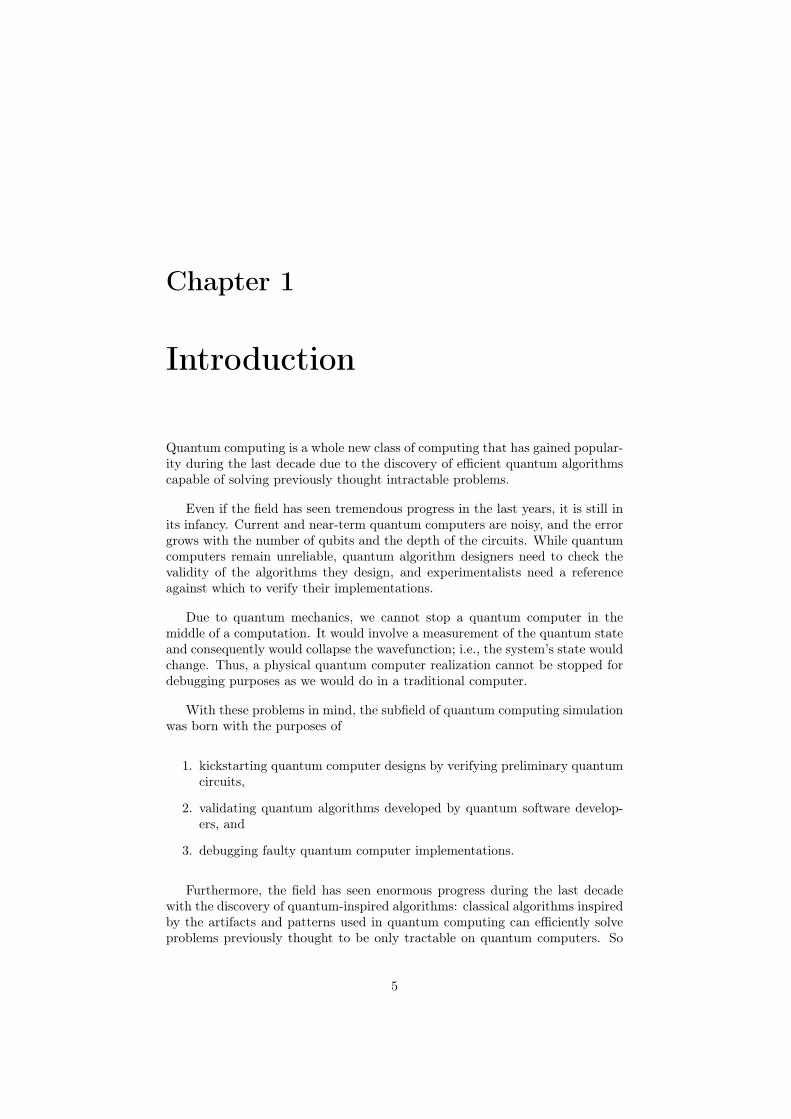
Quantum computing is a whole new class of computing that has gained popular-ity during the last decade due to the discovery of efficient quantum algorithmscapable of solving previously thought intractable problems.

Even if the field has seen tremendous progress in the last years, it is still inits infancy. Current and near-term quantum computers are noisy, and the errorgrows with the number of qubits and the depth of the circuits. While quantumcomputers remain unreliable, quantum algorithm designers need to check thevalidity of the algorithms they design, and experimentalists need a referenceagainst which to verify their implementations.

Due to quantum mechanics, we cannot stop a quantum computer in themiddle of a computation. It would involve a measurement of the quantum stateand consequently would collapse the wavefunction; i.e., the system’s state wouldchange. Thus, a physical quantum computer realization cannot be stopped fordebugging purposes as we would do in a traditional computer.

With these problems in mind, the subfield of quantum computing simulationwas born with the purposes of

1. kickstarting quantum computer designs by verifying preliminary quantumcircuits,

2. validating quantum algorithms developed by quantum software develop-ers, and

3. debugging faulty quantum computer implementations.

Furthermore, the field has seen enormous progress during the last decadewith the discovery of quantum-inspired algorithms: classical algorithms inspiredby the artifacts and patterns used in quantum computing can efficiently solveproblems previously thought to be only tractable on quantum computers. So

5

Chapter 1

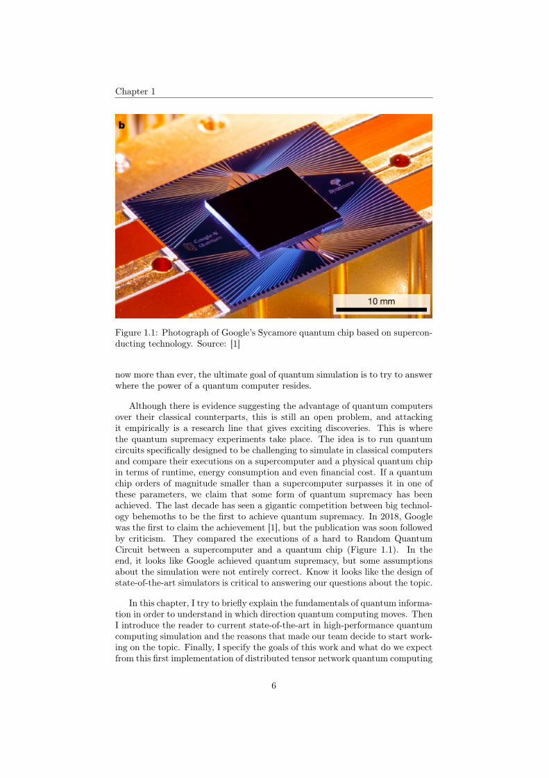
Figure 1.1: Photograph of Google’s Sycamore quantum chip based on supercon-ducting technology. Source: [1]

now more than ever, the ultimate goal of quantum simulation is to try to answerwhere the power of a quantum computer resides.

Although there is evidence suggesting the advantage of quantum computersover their classical counterparts, this is still an open problem, and attackingit empirically is a research line that gives exciting discoveries. This is wherethe quantum supremacy experiments take place. The idea is to run quantumcircuits specifically designed to be challenging to simulate in classical computersand compare their executions on a supercomputer and a physical quantum chipin terms of runtime, energy consumption and even financial cost. If a quantumchip orders of magnitude smaller than a supercomputer surpasses it in one ofthese parameters, we claim that some form of quantum supremacy has beenachieved. The last decade has seen a gigantic competition between big technol-ogy behemoths to be the first to achieve quantum supremacy. In 2018, Googlewas the first to claim the achievement [1], but the publication was soon followedby criticism. They compared the executions of a hard to Random QuantumCircuit between a supercomputer and a quantum chip (Figure 1.1). In theend, it looks like Google achieved quantum supremacy, but some assumptionsabout the simulation were not entirely correct. Know it looks like the design ofstate-of-the-art simulators is critical to answering our questions about the topic.

In this chapter, I try to briefly explain the fundamentals of quantum informa-tion in order to understand in which direction quantum computing moves. ThenI introduce the reader to current state-of-the-art in high-performance quantumcomputing simulation and the reasons that made our team decide to start work-ing on the topic. Finally, I specify the goals of this work and what do we expectfrom this first implementation of distributed tensor network quantum computing

6

Chapter 1

simulator.

1.1 Fundamentals of Quantum Information

The way quantum computing works is fundamentally different from how clas-sical computers work, that it is necessary to give a brief introduction. Thisintroduction skips many topics on quantum computing and focuses on the coreof the topic. Then, we refer the reader to [2] for a larger and deeper explanationof the field.

We first want to explain that the output of a quantum computer is not a value(like a bitstring) but a complex probability distribution. Let us view it from themost fundamental object: the qubit. Analogous to the classical world, a qubitis the smallest possible unit of quantum information. It is a vector representinga 2-state quantum system, but unlike its classical counterpart, the bit, its valueis not discrete but continuous due to the principle of quantum superposition.Technically speaking, a qubit can take any value from the 2-dimensional Hilbertspace H2.

|ψ〉 =

(α0

α1

)where αi ∈ C (1.1)

Given that a qubit represents a vector in a 2-dimensional vector space, manybases may represent it. The most popular basis in the field of quantum com-puting and quantum information is the computational basis.

|0〉 =

(10

)|1〉 =

(01

)(1.2)

However, others can be used, such as the polar basis.

|+〉 =1√2

(11

)|−〉 =

1√2

(1−1

)(1.3)

Thus the amplitudes α0, α1 are the values of the discrete complex probabilitydistribution in which α0 is related to the probability of measuring |0〉 and α1

is related to the probability of measuring |1〉. As the probability distribution islocated in a vector space, the probability distribution will differ in other bases.

|ψ〉 = α0 |0〉+ α1 |1〉 = α+ |+〉+ α− |−〉 (1.4)

But how are these quantum amplitudes α related to the probability of mea-suring a specific state? When we measure the state of the qubit, two thingshappen:

1. The qubit state vector is projected onto the basis vectors of the measure-ment operator.

7

Chapter 1

2. The projected values form a new classical probability distribution, and asample is taken from it.

After the measurement, the qubit changes and points to the measurementresult, also known as "wavefunction collapse." If the measurement is done ona given basis, then the probability of measuring each possible output is thesquared module of each amplitude on the given basis.

p(M(|ψ〉) = |0〉) = ||α0||2 p(M(|ψ〉) = |1〉) = ||α1||2 (1.5)

Operations on the qubit are performed through linear mappings (i.e., ma-trixes). The only requirements for an operator to be valid are that it must be(a) unitary (its norm must be one) and (b) Hermitian. Here we picture the Paulioperators, which are some of the most popular single-qubit quantum operators.

I =

(1 00 1

)X =

(0 11 0

)Y =

(0 −ii 0

)Z =

(1 00 −1

)(1.6)

As an enlightening example, the X operator is also known as the NOToperator as if it is applied to a qubit whose value is one of the computationalbasis, the qubit changes to the other computational basis vector.

X |0〉 = |1〉 X |1〉 = |0〉 (1.7)

When composing a system made out of several qubits, the axioms of quantummechanics assert that the state representing the system is the tensor product ofeach individual qubit system.

|Ψ〉 = |ψ1 . . . ψn〉 = |ψ1〉 ⊗ · · · ⊗ |ψn〉 (1.8)

Let us see it with an example. Imagine we have a system made out oftwo qubits. Then the state vector representing the composite system needs aquantum amplitude for each of the possible outcomes of the states of its qubits.So, for example, if both qubits are in state |0〉, then the amplitude of state |00〉is 1 and thus, the probability of measuring |0〉 in both qubits is also 1.

|00〉 = |0〉 ⊗ |0〉 =

1000

=

α00

α01

α10

α11

(1.9)

To summarizing, a quantum state can be seen as a discrete probability distri-bution where each probability has a complex phase. This phase, combined withits probabilistic nature, makes quantum computing so powerful. It lets probabil-ities of different outcomes interact constructively and destructively, somethingnot possible using classical probabilities.

8

Chapter 1

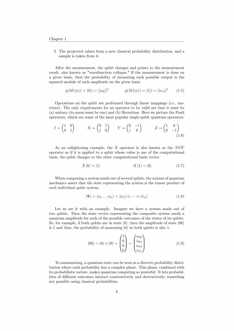
Figure 1.2: Circuit representing the Quantum Fourier Transform. Source: [2].

Operators are not limited operations to single-qubits. They can be con-structed that act on any number of qubits, but this is not done in practicein the field of quantum computing as any n-qubit operator can be decomposedinto a circuit of single- and double-qubit operators. As an enriching example, weshow below some of the most popular double-qubit quantum gates: controlledsingle-qubit gates C(O) and the SWAP gate.

C(O) =

1 0 0 00 1 0 00 0 O11 O12

0 0 O21 O22

SWAP =

1 0 0 00 0 1 00 1 0 00 0 0 1

(1.10)

By composing single- and double-qubit operators, we can build quantumcircuits that express quantum algorithms. These descriptions of circuits canthen be passed to the physical realization of quantum computers or quantumcomputing simulators.

1.2 Methods for Classical Simulation of Quan-tum Computing

Traditionally, there have been two methods for quantum computing simulation.

1.2.1 Schrödinger or Full state vector Simulators

This kind of simulators work by storing and evolving the whole state vector thatdescribes the n-qubit system.

|Ψ〉 = |ψ1〉 ⊗ |ψ2〉 ⊗ · · · ⊗ |ψn〉 (1.11)

The main advantage of this simulation method is that we know the value ofany quantum amplitudes at every step of the simulation, which is of great valuefor debugging a circuit or visualizing the quantum computation while studying

9

Chapter 1

Figure 1.3: Illustration of the partition schemes used to distribute the statevector. Source: [3].

the field as a student. However, it comes at the cost of exponential memoryusage with the number of qubits.

dim Ψ =

n∏i=1

dimψi = 2n (1.12)

Moreover, each quantum gate modifies every entry of the state vector, soevery operation is exponential in the number of qubits.

As memory requirements grow so fast, they soon need to split the statevector and distribute it along compute nodes. Thus, the partition scheme usedby simulators is a crucial component of their performance. Usually, the statevector is split equally along the nodes. “A common strategy to then evaluatea circuit is to pair nodes such that upon applying a single qubit gate, everyprocess must send and receive the entirety of its portion of the state vector toits paired process. The number of communications between paired processes, theamount of data sent in each and the additional memory incurred on the computenodes form a trade off. A small number of long messages will ensure that thecommunications are bandwidth limited, which leads to best performance in thecommunications layer. However this results in a significant memory overhead,due to the process having to store buffers for both the data it is sending andreceiving, and in an application area so memory hungry as quantum circuitsimulation this may limit the size of circuit that can be studied. On the otherhand many short messages will minimise the memory overhead as the messagebuffers are small, but will lead to message latency limited performance as thebandwidth of the network fabric will not be saturated. This in turn leads to poorparallel scaling, and hence again limits the size of the circuit under consideration,but now due to time limitations. Note that the memory overhead is at mosta factor 2, which due to the exponential scaling of the memory requirements,means only 1 less qubit may be studied.” [3] Some communication strategiesand their memory overheads and visualised in Figure 1.3.

10

Chapter 1

1.2.2 Schrödinger-Feynman Simulators

This kind of simulator is inspired by the many-worlds interpretation of quantummechanics and the Path-Integral or Feynman formalism. The idea behind thisis that a circuit is split into two parts by a cut on the lattice. Then double-qubit gates on the cut are then decomposed using the Schmidt decomposition.For example, if the Schmidt rank of the gate is m and the number of gates onthe cut is k, then we can precisely simulate the circuit by simulating all themk paths and summing the results [4, 5]. The execution time is then of com-plexity O

((2n1 + 2n2)mk

)where n1, n2 are the number of qubits of each part.

The evaluation of each part may be performed by Full state vector simulatorsindependently. This cuttings may be performed recursively on each part untiln1 = n2 = 1. At this point, the evaluation of a part is straightforward, but thenumber of instances is exponential in the number of double-qubit gates. Therecommended way of using this kind is to split the circuit until the size of eachpartial state vector fits into memory. This way, communication between nodesis needed during the computation.

This simulation method’s advantages are that the amount of required spaceis exponentially lower than with Schrödinger-like simulators. In addition, theevaluation of different instances exhibits an embarrassingly parallel pattern.Unfortunately, this comes at the cost of an exponential number of instancesthat grow with the number of double-qubit gates.

To sum up, traditionally, there have been two kinds of simulators for quan-tum computing: Full state vector simulators, which scale well on circuit depthbut are heavily limited on the number of qubits and hybrid Schrödinger-Feynmansimulators that scale well on the number of qubits but fail to scale with the cir-cuit depth. A new method has been proposed that keeps the strengths of bothtypes, but at the same time, it may be capable of overcoming their most criticalweaknesses: tensor networks.

1.3 Tensor Networks

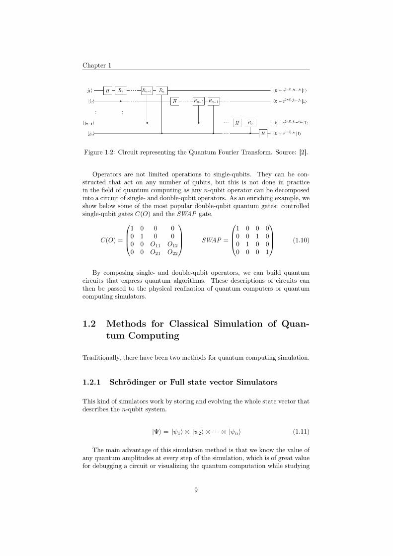
A tensor is an algebraic object that describes a multilinear relationship betweena set of vector spaces. It can be seen as a higher-order generalization of lin-ear transformations. It can be represented by a n-dimensional1 array with anassociated linear algebra. For example, a scalar can be seen as a 0-order ten-sor, a vector as a 1-order tensor, a matrix as a 2-order tensor and so on. OnFigure 1.4, we show a illustration relating index summation notation, graphical

1Note that the semantics of the word dimension may vary depending on the context. Forexample, in the computing world, when we refer to the dimensionality of an array, we arespeaking about the components of the array or the number of values we need to locate anelement in the array precisely. Whereas in the physics and mathematics worlds, this is calledthe rank or order of the tensor. A better translation of the array dimension to the mathematicsworld is the tensor index or label, as we use labels to identify each array dimension. Finally,when we refer to the dimensionality of a given tensor index, it would be called the size of anarray dimension in the programming world.

11

Chapter 1

notation and array visualization.

Figure 1.4: Cheatsheet diagrams of low-order tensor representations. Source:[6]

A more precise way of viewing double-qubit tensors are 4-order tensors, with2 input indexes and 2 output indexes, 1 per qubit. In the following equation,we show an example of the quantum computation using the tensor summation.Two qubits, ψi and φj , are being applied a set of quantum gates, representedby the 2-order tensor H and the 4-order tensor CX, using the tensor summationnotation. The result is a 2-order tensor Ψkl that represents the entangled stateof the two qubits.

Ψkl =∑ijklmo

ψiφjHikHjlCXklmoHmpHoq (1.13)

As we add more tensors with higher order and start connecting all the vectorspaces between them, equations start getting confusing. In order to get a cleanervisualization of tensor equations, a graphical notation known as tensor networksis used [7, 8, 9, 10, 11] where tensors are represented by nodes in a graph andedges represent the tensor indexes connecting the vector spaces of the tensors.Using the tensor network notation, we would have the graph in Figure 1.5 for

12

Chapter 1

Figure 1.5: Tensor network diagram of Equation 1.13.

Equation 1.13.

So transforming a quantum circuit into a tensor network is straightforward.Moreover, the full quantum state vector simulation paradigm can be seen as aparticular case of tensor network where the input quantum state has alreadybeen combined into an n-order tensor.

Evaluation of tensor networks is not done directly: New intermediate tensorsare generated by partial evaluation of a label in the summation. Using the tensornetwork notation, it can be seen as if two connected nodes are merged into oneand the edges connecting both collapse. As systems become larger and circuitsbecome deeper, these intermediate tensors may grow larger as tensors are moreconnected. Furthermore, the size of these intermediate tensors will vary withthe order in which we perform the contraction. Finding the optimal contractionpath is known to be NP-hard for general tensor networks, but some heuristicsare known to yield good enough solutions for medium-sized networks [12, 13].

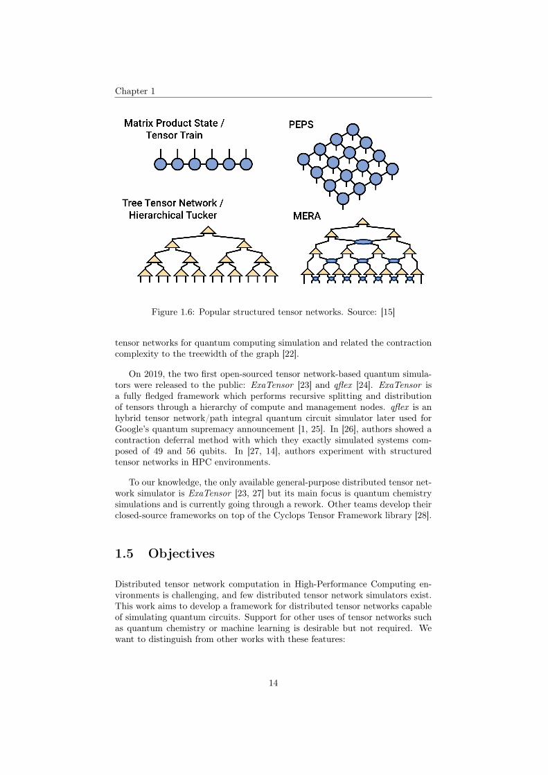
In addition, tensor networks can be used to represent factorizations of quan-tum states. When developing its evolution over a circuit, their structures areconserved by repeatedly contracting and factorizing their tensors. As multiplequbit operators increase the vector space between tensors, structured tensor net-works should also grow exponentially in space as they evolve. But by employingrank-k factorizations instead of exact ones, they obtain approximated repre-sentations in polynomial-space [8, 14]. Some of the most promising structuredtensor networks are shown in Figure 1.6.

1.4 State of the Art

During the last decade, many simulators have been developed, most of whichare of the Full state vector kind [16, 17, 18, 19, 3, 20, 21]. Differences betweenthem lie in implementation optimizations targeting different architectures (e.g.,GPUs), quantum circuits optimizations (e.g., gate fusion) or analysis statisticsbut none of them has yet surpassed the barrier of 45 qubits simulation. Even ifnew supercomputers grow significantly in size, they are not expected to improvemuch.

The use of tensor networks for quantum computing simulation is relativelynew. In 2009, Igor L. Markov and Yaoyun Shi first acknowledged the power of

13

Chapter 1

Figure 1.6: Popular structured tensor networks. Source: [15]

tensor networks for quantum computing simulation and related the contractioncomplexity to the treewidth of the graph [22].

On 2019, the two first open-sourced tensor network-based quantum simula-tors were released to the public: ExaTensor [23] and qflex [24]. ExaTensor isa fully fledged framework which performs recursive splitting and distributionof tensors through a hierarchy of compute and management nodes. qflex is anhybrid tensor network/path integral quantum circuit simulator later used forGoogle’s quantum supremacy announcement [1, 25]. In [26], authors showed acontraction deferral method with which they exactly simulated systems com-posed of 49 and 56 qubits. In [27, 14], authors experiment with structuredtensor networks in HPC environments.

To our knowledge, the only available general-purpose distributed tensor net-work simulator is ExaTensor [23, 27] but its main focus is quantum chemistrysimulations and is currently going through a rework. Other teams develop theirclosed-source frameworks on top of the Cyclops Tensor Framework library [28].

1.5 Objectives

Distributed tensor network computation in High-Performance Computing en-vironments is challenging, and few distributed tensor network simulators exist.This work aims to develop a framework for distributed tensor networks capableof simulating quantum circuits. Support for other uses of tensor networks suchas quantum chemistry or machine learning is desirable but not required. Wewant to distinguish from other works with these features:

14

Chapter 1

• Compatibility with the Python ecosystem: Every discovery in thefield is then made available to scientists as libraries in the most usedlanguage for scientific research, Python. We would want to benefit fromsuch development and offer scientists a semi-automatic way to distributesimulations in supercomputers.

• Architecture-agnostic implementation: With a diverse set of clustersand accelerators, we want a portable application that efficiently works inall architectures.

• Fault-tolerance for Exascale computing: As we approach the Exas-cale era, supercomputers are built with an increasing number of comput-ers and start getting faults during executions more frequently which is notpermissible for day-lasting simulations.

• Profiling support: Optimal parallelization and distribution of tensornetworks is not a well-understood problem yet. Being able to measure andvisualize how the parallelization is performed gives us a good advantagefor improvement.

1.6 Contributions of this work

The main contributions of this work to the state-of-the-art can be enumeratedas the following:

• Design of a partitioning layout for distributed tensors: Few dis-tributed tensor libraries exist and do not consistently explain how theywork. Based on their spare ideas, we designed a layout to divide tensorsinto blocks and developed algorithms to perform tensor algebra on suchblocked layout.

• Implementation of a general purpose distributed tensor networklibrary: We developed a Python library for distributed computation oftensors on top of the COMPSs programming model, that fulfills all of ourgoals.

• Integration with the ecosystem We integrated our library with theecosystem of tensor libraries. Specifically we integrate with opt_einsum[12] and quimb [29] libraries, built on top of the standard numpy libraryfor n-dimensional arrays.

• Implementation of an asynchronous SVD with the COMPSsframework: As multiple concurrent gates will be applied in structuredtensor networks, we need an asynchronous implementation of the SVD toavoid locking the main thread. Synchronization may be occur due to SVDalgorithm being iterative. We modified the SVD implementation of thedislib library [30] for such needs by using nested tasks.

• Discovery of an algorithm for partitioning of tensors: Which andhow tensors from a circuit have to be sliced is not a trivial problem. Ifthe slicing is too fine grained, we will end up with an exponential numberof short tasks and high overhead. If the slicing is too coarsed, there may

15

Chapter 1

not be enough tasks to fully exploit parallelism. We found out that thetensor slicing algorithm is a good heuristic for deciding the partitioningof tensors into tensor blocks and apply it for automatic slicing of tensorsgiven some parameters.

• Exploratory analysis of partitioning configuration: We evaluatethe performance of our application for different block sizes and communi-cation backends, giving a first hint on how efficient simulations should beperformed.

1.7 Outline

This document is organized in the following way:

• Chapter 2. Designs explains the partitioning layout we developed forblock tensor algebra. It also further develops algorithms for performingcommonly-used tensor operations on the new layout. Finally, we describean algorithm that decides the partitioning of tensors from a circuit.

• Chapter 3. Implementation shows the implementation of the algo-rithms presented in the previous chapter using the COMPSs program-ming model. Section 1 gives a brief explanation of what is the COMPSsframework, Section 2 presents the implementation of the tensor algebrausing COMPSs and Section 3 explains the modifications we needed to becompatible with the Python ecosystem. This last section may be skippedif the reader wants to focus on the results of this work.

• Chapter 4. Evaluation We show three circuits known to be hard tosimulate and then evaluate the performance of our application with them.

• Chapter 5. Conclusion The document ends with a summary of theachievements accomplished in this work, opinions regarding state-of-the-art and a list of ideas that could not be implemented for this thesis dueto technical and time constraints.

16

Chapter 2

Design

From a computational point of view, a tensor can be represented by a n-dimensional numerical array. In our case, the size of the array dimensions is setto 2 and, the number of dimensions will grow as we simulate circuits with anincreasing depth and number of qubits. Due to this, the memory required bya tensor will grow exponentially with the number of array dimensions. Currentclusters are provided with around 100 to 1000 GiB per node, which by assumingeach element is a single-precision complex number (8 bytes), would let us storea single tensor of rank 33-36 at much. If we want to simulate circuits whoseintermediate tensors have a higher rank, we need a layout for dividing the tensorand distributing their content. Furthermore, we need a way to decide how toslice the tensor optimally. This chapter tries to answer both of these questionsby presenting a layout for distributed block tensor algebra and an algorithm forselecting tensor indexes to be sliced.

2.1 Dimension Extents layout

Taking inspiration from the block linear algebra, authors in [31, 28] developeda block tensor layout called dimension extents. An “extent” is a synonym for“range” or “slice”. Hence, a dimension extent refers to the range of coordinatesin a dimension which this block contains 1

T [bi1 : ei1 , . . . ,bin : ein ] 0 ≤ bi < ei ≤ dim(i) ∀i ∈ I (2.1)

If we group the beginning and the end of the ranges into vectors b and e,then the space contained by the tensor block is a hyperrectangle whose more

1Notice here that the “dimension” in “dimension extents” does not have the same conno-tation as in the phrase "n-dimensional array"; it has the semantics used in the mathematicaland physics worlds. Here “dimension” refers to the size in elements of a given value of an-coordinate for a n-dimensional array.

17

Chapter 2

distant vertices are located in b and e (Figure 2.1). The dimensions of thetensor block are found to be the longest diagonal of the hyperrectangle, definedas block_shape = e− b. Something noteworthy is that the volume of the spaceit represents is just the product of its components.

Figure 2.1: Hyperrectangle of a tensor block defined by vectors b and e.

If we set a fixed block_shape for all tensor blocks, then we get an uniformgrid of blocks and can get rid of the b and e vectors (Figure 2.2).

Figure 2.2: Tensor sliced into an uniform grid of blocks

2.1.1 Permutation

Permutation is the operation of reordering the indexes or labels of a tensor. Thesimplest example of a tensor permutation is a matrix transposition, in which a2-order tensor has its two indexes swapped.

(Mij)T = Mji (2.2)

From the mathematical perspective, this operation does not have much com-plexity as it is just a permutation of some labels (the indexes). However, fromthe computational point of view, it implies data permutation in memory. Inthe last years, high-performance libraries have appeared in the literature whichwork on dense arrays located on shared memory [32, 33, 34]. In order to makethem work with distributed arrays, we need to analyze the problem.

18

Chapter 2

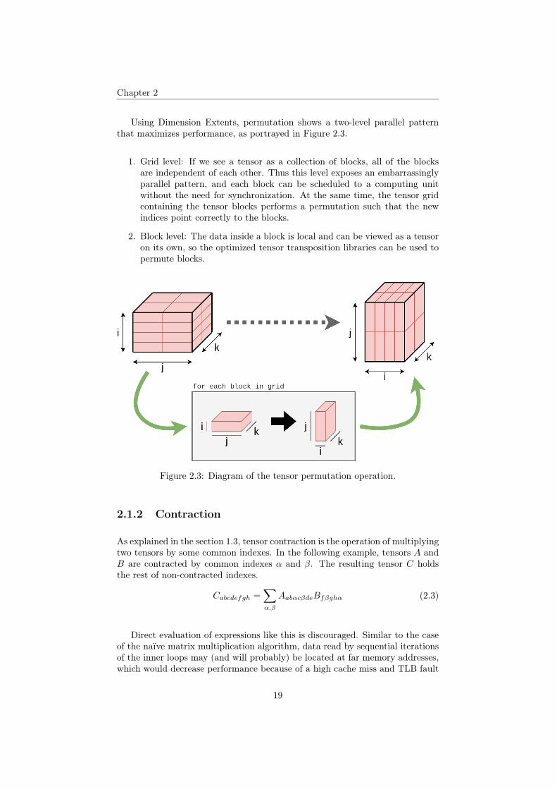
Using Dimension Extents, permutation shows a two-level parallel patternthat maximizes performance, as portrayed in Figure 2.3.

1. Grid level: If we see a tensor as a collection of blocks, all of the blocksare independent of each other. Thus this level exposes an embarrassinglyparallel pattern, and each block can be scheduled to a computing unitwithout the need for synchronization. At the same time, the tensor gridcontaining the tensor blocks performs a permutation such that the newindices point correctly to the blocks.

2. Block level: The data inside a block is local and can be viewed as a tensoron its own, so the optimized tensor transposition libraries can be used topermute blocks.

Figure 2.3: Diagram of the tensor permutation operation.

2.1.2 Contraction

As explained in the section 1.3, tensor contraction is the operation of multiplyingtwo tensors by some common indexes. In the following example, tensors A andB are contracted by common indexes α and β. The resulting tensor C holdsthe rest of non-contracted indexes.

Cabcdefgh =∑α,β

AabαcβdeBfβghα (2.3)

Direct evaluation of expressions like this is discouraged. Similar to the caseof the naïve matrix multiplication algorithm, data read by sequential iterationsof the inner loops may (and will probably) be located at far memory addresses,which would decrease performance because of a high cache miss and TLB fault

19

Chapter 2

ratios. Furthermore, developing optimized implementations for different con-traction patterns is futile as the number of possible contraction patterns tooptimize is immense.

There is a way to circumvent this problem and maximize performance. Bypermuting tensor indexes so that contracting indexes are grouped on one side,and non-contracting indexes are grouped on the other side, tensors can be viewedas matrices,

Ti1, . . . , it︸ ︷︷ ︸M

it+1, . . . , in̄︸ ︷︷ ︸N

≡ TMN t ∈ N (2.4)

and contraction can be performed by calling optimized matrix multiplicationroutines of optimized BLAS libraries.

Cmn =∑k

AmkBkn (2.5)

It is important to notice that once the permutation has been performed,treating the tensor as a matrix is just a matter of view as the tensor has notbeen modified. Furthermore, the volumes of the tensor and its tensor blocks areconserved.

dim(M) =∏i≤t

dim(ai) dim(N) =∏

t<j≤n̄

dim(aj) (2.6)

When performing the matrix multiplication, we have to be careful about thedimension extents layout. Due to the slicing in a higher dimensionality spaceand its projection to a 2D space (the matrix), different layers of the tensor blocksare located at periodically distanced 2D coordinates of the matrix. However, asa block is stored as a whole as a chunk of memory, if we try to concatenate thetensor blocks reshaped in matrix blocks, we would then have a permuted versionof the matrix. In Figure 2.4, the reader can find an example of a 3-order tensormapped into a matrix in which colors distinguish tensor blocks. Theoretically,permutation should preserve the tensor structure after contraction but we haveyet to test it. So we decided to perform only the permutation at the block level,as explained below.

The instructions for performing a contraction using the dimension extentslayout are the following:

1. For each output block in tensor C, we select the blocks from A and Bneeded to compute the resulting block. These blocks are chosen by match-ing coordinates from non-contracting indexes which in the example of Fig-ure 2.5a are indexes j and m.

2. Once the input blocks of A and B have been selected, we group them inpairs by matching the coordinates of contracting indexes. In the exampleshown in Figure 2.5b, the contracting indexes are indexes i and k.

20

Chapter 2

Figure 2.4: Mapping from 3-order tensor to matrix. Tensor blocks are distin-guished by color.

3. Each of the pairwise coupled indexes when contracted will compute apartial contribution to the output block (Figure 2.5c).

4. In order to perform the contraction of the pairwise couple blocks, we maytranspose the tensors, reshape them into matrices and then do a matrixmultiplication (Figure 2.5d).

5. All the partial blocks are summed and we have the output block of C(Figure 2.5e).

Finally, we have to ensure that the block sizes for the contracting indexes dofit. Additionally, we have to compute the grid and block_shape of the resultingtensor. We recommended to lay out their values of the involved tensors as inTable 2.1 such that we assert that the components for the contracting indexesα, β coincide and the values for the non-contracting indexes a, b, c, d, e, f, g, h ofthe resulting tensor C are computed by rows.

a b c d e f g h α βA 2 2 2 1 1 - - - 2 2B - - - - - 1 1 1 2 2C 2 2 2 1 1 1 1 1 - -

Table 2.1: Example of computing the grid or block_shape for a given tensorcontraction.

2.1.3 Schmidt decomposition

The Schmidt decomposition is a factorization of a quantum state as a tensorproduct of two inner product spaces. It can be thought as the opposite operationto the tensor contraction. Let H1, H2 be Hilbert spaces of dimension n and m,n ≥ m. For any a vector w in the space ofH1⊗H2, there exist some orthonormalbases ui ⊂ H1, vi ⊂ H2 such that Equation 2.7 is fulfilled and αi are real, non-negative scalars.

21

Chapter 2

(a) Input blocks selection

(b) Pairwise coupling of tensor blocks

(c) Partial Tensor Block Contraction

(d) Partial Tensor Block Contraction as Matrix Multiplication

(e) Sum of partial block contractions

Figure 2.5: Steps of Tensor Contraction using Dimension Extents

22

Chapter 2

w =

n∑i=1

m∑j=1

βijei ⊗ fj (2.7)

The Schmidt decomposition is a critical operation in structured tensor net-works as when two qubit tensors are contracted to apply a double-qubit gate, weneed then to decompose the resulting tensor to recover the tensors representingthe two qubits and, in this way, preserve the topology of the network.

Similar to the tensor contraction in Section 2.1.2, here there is also a trick inorder to compute it using linear algebra operations. Suppose we permute andreshape the tensor into a matrix so that the two tensor index groups are laid outas rows and columns of the matrix. In that case, the Schmidt decomposition isequivalent to the Singular Value Decomposition (SVD).

Due to the dimension extents layout, the tensor-mapped-matrix will alsohappen to be permuted. Luckily, we found out that SVD is invariant to row,column permutations (Theorem 1) and as such its unaffected by the layout.

Theorem 1 (Permutation Invariance of the Singular Value Decomposition).Given matrix A and its SVD A = UΣV †. Let Rr, Rc be permutation matrixes.Let A′ = RrARc be a row (Rr) and column (Rc) permutation of matrix A, thenits Singular Value decomposition of is,

U ′ = RrU Σ′ = Σ V ′ = RcV (2.8)

Proof. We first replaceA in the definition ofA′ as a row and column permutationof A with its Singular Value Decomposition.

RrARc = RrUΣV †Rc (2.9)

As U and V describe a pair of orthonormal basis on their column vectors,RrU and RcV are just some row reorderings of these vectors. The vectors donot change: it is just a reindexing of the components of the vectors. But mostimportantly, the indexing of the column vectors keep invariant so the singularvalues in Σ are not permuted.

2.1.4 Rechunk

Although not a mathematical operation per se, rechunk is needed from a com-putational point of view. A chunk is equivalent to a block of data so rechunkingmeans the action of changing the size of our tensor blocks. Unlike reshaping,which changes the size of each tensor dimension without changing the datanor the volume represented in the tensor space, rechunking changes the spacerepresented by the block in the tensor.

23

Chapter 2

For example, as explained in Section 2.1.2, we may perform tensor contrac-tion by permuting contracting indexes on one side and non-contracting indexeson the other, and then performing matrix multiplication. This action of takingthe permuted tensor and viewing it as a matrix for matrix multiplication wouldbe a reshape. Data does not change, it is only a matter of view. A rechunksplits and merges tensor blocks so resulting blocks are different.

2.2 The SliceFinder Algorithm

Due to the complexity of distributing tensors, researchers developed the ten-sor slicing or cuttings technique [5, 24] to perform tensor network contractionslocally. The idea behind is inspired by the Feynman-like simulation method.In this case, vector spaces of selected tensor indexes are projected into a singlevalue, usually a basis of the vector space, and the tensors connected by suchlabel are then disconnected. If we contract such sliced network, we will end upwith a partial result. As in the Path Integral paradigm, by summing the resultsof the contraction of all possible network projections, one ends up with an exactresult. In the end, as we are dealing with the summation of network projections,tensor slicing can is equivalent to the decomposition of the network into a sumover the selected labels.

Figure 2.6: Tensor cutting or slicing example. Source: [13]

When we repeatedly contract a sliced tensor network, the contraction ofnon-sliced tensors is redundant. Depending on the selected labels, the overheadof the redundant contraction can be rather large. We also have to take aboutwhich label to project. If the sliced labels are not correctly chosen, the interme-diate tensors can grow large and surpass the available memory. Furthermore, ifwe select too many labels, the number of instances to simulate will grow up ex-ponentially. Luckily, the cotengra [13] library provides us with an optimizationalgorithm, called SliceFinder, for solving this issue.

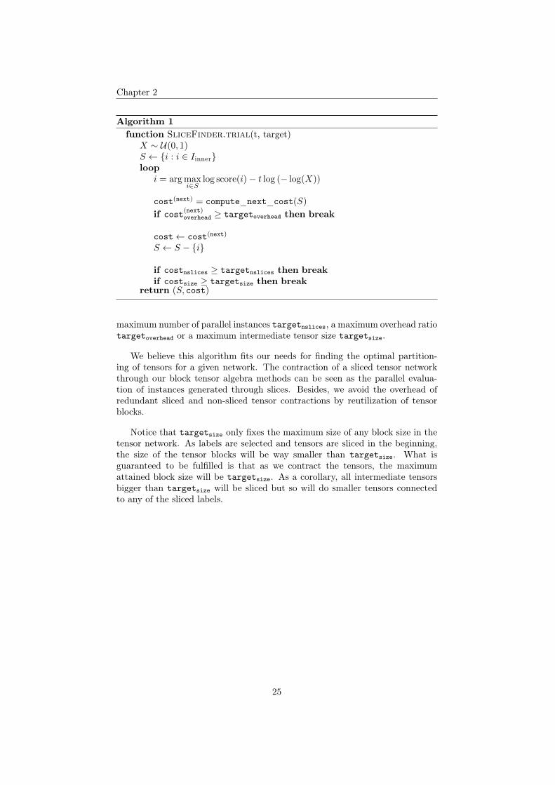
A pseudocode of the algorithm is shown in Algorithm 1. The algorithmstarts by choosing all inner indexes of the network as a candidate solution oneach trial. Then, iteratively takes out the label, which adds less overhead tothe computation. Finally, the loop stops when one of the target threshold hasbeen surpassed.

As shown in Algorithm 1, we may configure the algorithm by setting a

24

Chapter 2

Algorithm 1function SliceFinder.trial(t, target)

X ∼ U(0, 1)S ← {i : i ∈ Iinner}loop

i = arg maxi∈S

log score(i)− t log (− log(X))

cost(next) = compute_next_cost(S)

if cost(next)overhead ≥ targetoverhead then break

cost← cost(next)

S ← S − {i}

if costnslices ≥ targetnslices then breakif costsize ≥ targetsize then break

return (S, cost)

maximum number of parallel instances targetnslices, a maximum overhead ratiotargetoverhead or a maximum intermediate tensor size targetsize.

We believe this algorithm fits our needs for finding the optimal partition-ing of tensors for a given network. The contraction of a sliced tensor networkthrough our block tensor algebra methods can be seen as the parallel evalua-tion of instances generated through slices. Besides, we avoid the overhead ofredundant sliced and non-sliced tensor contractions by reutilization of tensorblocks.

Notice that targetsize only fixes the maximum size of any block size in thetensor network. As labels are selected and tensors are sliced in the beginning,the size of the tensor blocks will be way smaller than targetsize. What isguaranteed to be fulfilled is that as we contract the tensors, the maximumattained block size will be targetsize. As a corollary, all intermediate tensorsbigger than targetsize will be sliced but so will do smaller tensors connectedto any of the sliced labels.

25

Chapter 3

Implementation

In this chapter, we aim to explain the implementation details of our applica-tion. We decided to implement our compute kernels as tasks of the COMPSsprogramming model. This way we can forget about the low-level parallelizationtechnicalities and focus on exposing the parallelization opportunities.

3.1 Task and data distribution with COMPSs

COMP Superscalar (COMPSs) [35, 36, 37] is a framework and task-based pro-gramming model developed by the Workflows and Distributed Computing re-search group at the Barcelona Supercomputing Center with the following keycharacteristics:

• Sequential programming: COMPSs takes parallelization and distribu-tion aspects, such as thread creation and synchronization, data distribu-tion, messaging or fault tolerance.

• Infrastructure agnosticism: COMPSs abstracts applications from theunderlying distributed infrastructure making applications portable be-tween infrastructures with diverse characteristics.

• Bindings for standard programming languages: COMPSs applica-tions can be developed in Java, Python and C/C++.

COMPSs is supported by a runtime system that manages several aspectsof the applications’ execution. Some essential functionalities managed by theruntime are:

• Task Dependency Analysis: Tasks are the basis for parallelism inCOMPSs. The runtime automatically finds the data dependencies be-tween tasks based on the direction of their parameters. With this infor-

26

Chapter 3

mation, it dynamically builds a task dependency graph scheduled by theruntime when they are free of dependencies.

• Data Synchronization: Data accesses from the application’s main pro-gram are automatically synchronized by the runtime when necessary.

• Resource Management: For Cloud environments, the runtime featuresa set of pluggable connectors, each implementing the interaction of theruntime with a particular IaaS Cloud provider. The number of reservedvirtual resources can be elastically adapted to the task load that the run-time is processing.

• Job & Data Management: The runtime is in charge of performing re-mote execution of tasks and the data transfers. It provides an extensibleinterface for supporting several protocols for Job and Data Management.In the current release, two adaptors are implemented: the Non-blockingI/O, which offers high performance in secured environments, and the GATadaptor, which offers interoperability with diverse kinds of Grid middle-ware.

COMPSs is also complemented with a set of tools that eases development,executing monitoring and post-mortem performance analysis.

3.1.1 The @task decorator

In order to make an application work with COMPSs, the developer has to markthe compute kernels as tasks. Any call to a function marked with the @taskdecorator will be handled by COMPSs and executed in a free distributed workerselected by the scheduler. The runtime will also detect if any of the parametersis not managed by the runtime and upload it accordingly.

1 @task()2 def add(a,b):3 return a + b

Listing 3.1: Example of the @task decorator.

The user can specify set the type and dependency direction of the taskparameters as arguments of the @task decorator. The allowed parameter typesare:

• Primitive types

• Strings

• Objects (instances of classes, dictionaries, lists, tuples, . . . )

• Files

• Streams

• IO streams

And the dependency directions are:

27

Chapter 3

• Read-only (IN)

• Read-write (INOUT)

• Write-only (OUT)

• Concurrent (CONCURRENT)

• Conmutative (CONMUTATIVE)

COMPSs automatically detects the parameter type for primitive types, stringsand objects, while the user needs to specify it for files. If unspecified, COMPSswill default the parameter to the IN dependency direction. There is also a groupof COLLECTION kind of directions that allow the detection of COMPSs managedobjects inside a collection, such as a list.

1 @task(a=INOUT , b=IN)2 def add_inplace(a,b):3 a += b

Listing 3.2: Example of COMPSs dependency types setting.

3.1.2 Communication backend

COMPSs’ distribution of task parameters works by serialization of objects intofiles. This way, COMPSs attains fault-tolerance against task failures. If theworking directory is mounted onto a distributed filesystem, then data broad-casting is also obtained without much effort.

At the BSC installations, COMPSs counts with a pair of mounted filesystemsover GPFS, gpfs_scratch and gpfs_home, and can also work using local disk,in which case COMPSs will unicast data through SSH to requesting workers.Usually, gpfs_scratch is preferred over gpfs_home due to a higher number ofreplica servers that offer higher bandwidth and local disk is preferred over GPFSif the reutilization of the data objects is low.

3.2 Implementation of the tensor algebra

This section aims to explain the integration of COMPSs with our computekernels and how we abstracted a distributed n-dimensional block array whosedata is managed by the COMPSs runtime.

In order to jointly manage the blocks a sliced tensor, we developed a Tensorclass that stores and coordinates the grid of blocks. We used numpy’s [38]ndarray for representing the n-dimensional arrays of the grid and blocks. Inthe case of a block, the ndarray stores numerical values. While in the case ofthe grid, it stores references to the block objects managed by the COMPSsruntime.

28

Chapter 3

3.2.1 Array Initialization

The first type of tasks we need is the ones that initialize or upload data toCOMPSs. For this work, we created three simple tasks that generate an arrayin the COMPSs address space: block_full (Listing 3.3), which creates anndarray filled with a value, block_rand (Listing 3.4) that creates a ndarraywith random floating-point numbers and block_pass (Listing 3.5), which is justa hack to upload arrays to the COMPSs runtime and get a reference to it.

1 @task(returns=np.array)2 def block_full(shape , value , dtype , order=’F’):3 return np.full(shape , value , dtype , order)

Listing 3.3: Code of the block_full task.

1 @task(returns=np.array)2 def block_rand(shape):3 return np.asfortranarray(np.random.random_sample(shape))

Listing 3.4: Code of the block_rand task.

1 @task(block=IN, returns=np.ndarray)2 def block_pass(block):3 return block

Listing 3.5: Code of the block_pass task.

3.2.2 Permutation

The numpy.transpose routine permutes the n-dimensional array block. How-ever, as stated in the documentation, it will try to return a view rather than anew array with the permuted data. By calling to numpy.asfortranarray, weforce the view to turn into a copy of the array and perform the operation.

1 @task(block=IN, returns=numpy.ndarray)2 def block_transpose(block: numpy.ndarray , permutator):3 return np.asfortranarray(numpy.transpose(a, permutator))

Listing 3.6: Code of the block_transpose task.

3.2.3 Contraction

As explained in Section 2.1.2, tensor contraction is probably our most criticaloperation. In Listing 3.7 our blocked implementation of the tensordot routineis shown. We decided implement that sequentially executes each pairwise blocktensor contraction as it minimizes the memory usage.

1 @task(a={Type: COLLECTION_IN , Depth: 1},2 b={Type: COLLECTION_IN , Depth: 1},3 returns=np.ndarray)4 def block_tensordot(a, b, axes):5 return sum(np.tensordot(ba , bb , axes) for ba , bb in zip(a, b))

Listing 3.7: Code of the block_tensordot task.

29

Chapter 3

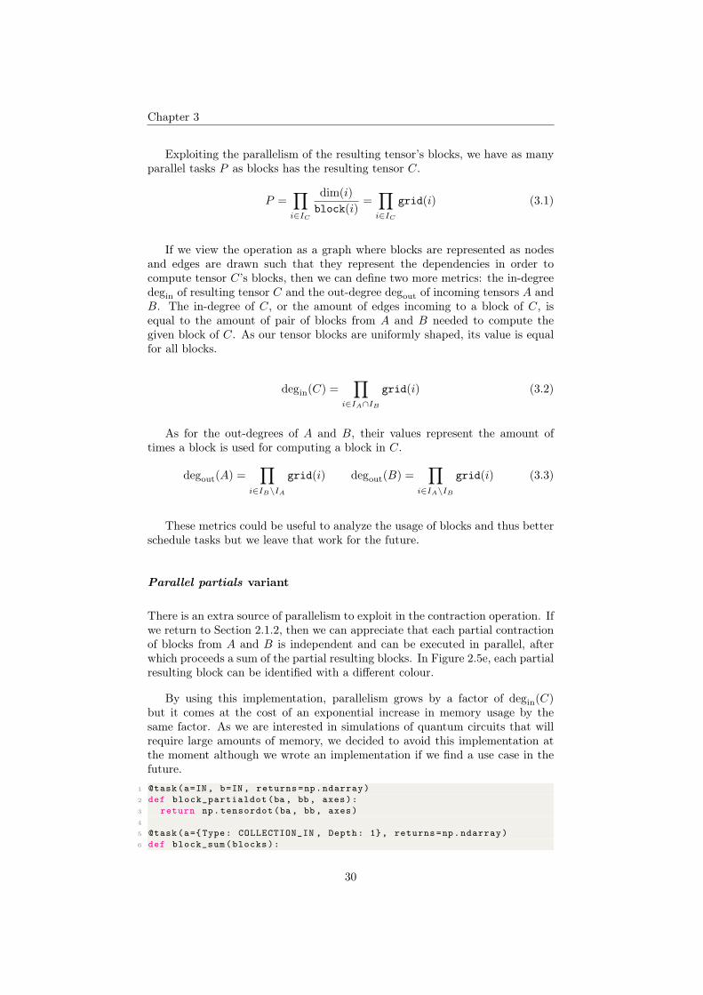
Exploiting the parallelism of the resulting tensor’s blocks, we have as manyparallel tasks P as blocks has the resulting tensor C.

P =∏i∈IC

dim(i)

block(i)=∏i∈IC

grid(i) (3.1)

If we view the operation as a graph where blocks are represented as nodesand edges are drawn such that they represent the dependencies in order tocompute tensor C’s blocks, then we can define two more metrics: the in-degreedegin of resulting tensor C and the out-degree degout of incoming tensors A andB. The in-degree of C, or the amount of edges incoming to a block of C, isequal to the amount of pair of blocks from A and B needed to compute thegiven block of C. As our tensor blocks are uniformly shaped, its value is equalfor all blocks.

degin(C) =∏

i∈IA∩IB

grid(i) (3.2)

As for the out-degrees of A and B, their values represent the amount oftimes a block is used for computing a block in C.

degout(A) =∏

i∈IB\IA

grid(i) degout(B) =∏

i∈IA\IB

grid(i) (3.3)

These metrics could be useful to analyze the usage of blocks and thus betterschedule tasks but we leave that work for the future.

Parallel partials variant

There is an extra source of parallelism to exploit in the contraction operation. Ifwe return to Section 2.1.2, then we can appreciate that each partial contractionof blocks from A and B is independent and can be executed in parallel, afterwhich proceeds a sum of the partial resulting blocks. In Figure 2.5e, each partialresulting block can be identified with a different colour.

By using this implementation, parallelism grows by a factor of degin(C)but it comes at the cost of an exponential increase in memory usage by thesame factor. As we are interested in simulations of quantum circuits that willrequire large amounts of memory, we decided to avoid this implementation atthe moment although we wrote an implementation if we find a use case in thefuture.

1 @task(a=IN, b=IN , returns=np.ndarray)2 def block_partialdot(ba, bb, axes):3 return np.tensordot(ba , bb , axes)4

5 @task(a={Type: COLLECTION_IN , Depth: 1}, returns=np.ndarray)6 def block_sum(blocks):

30

Chapter 3

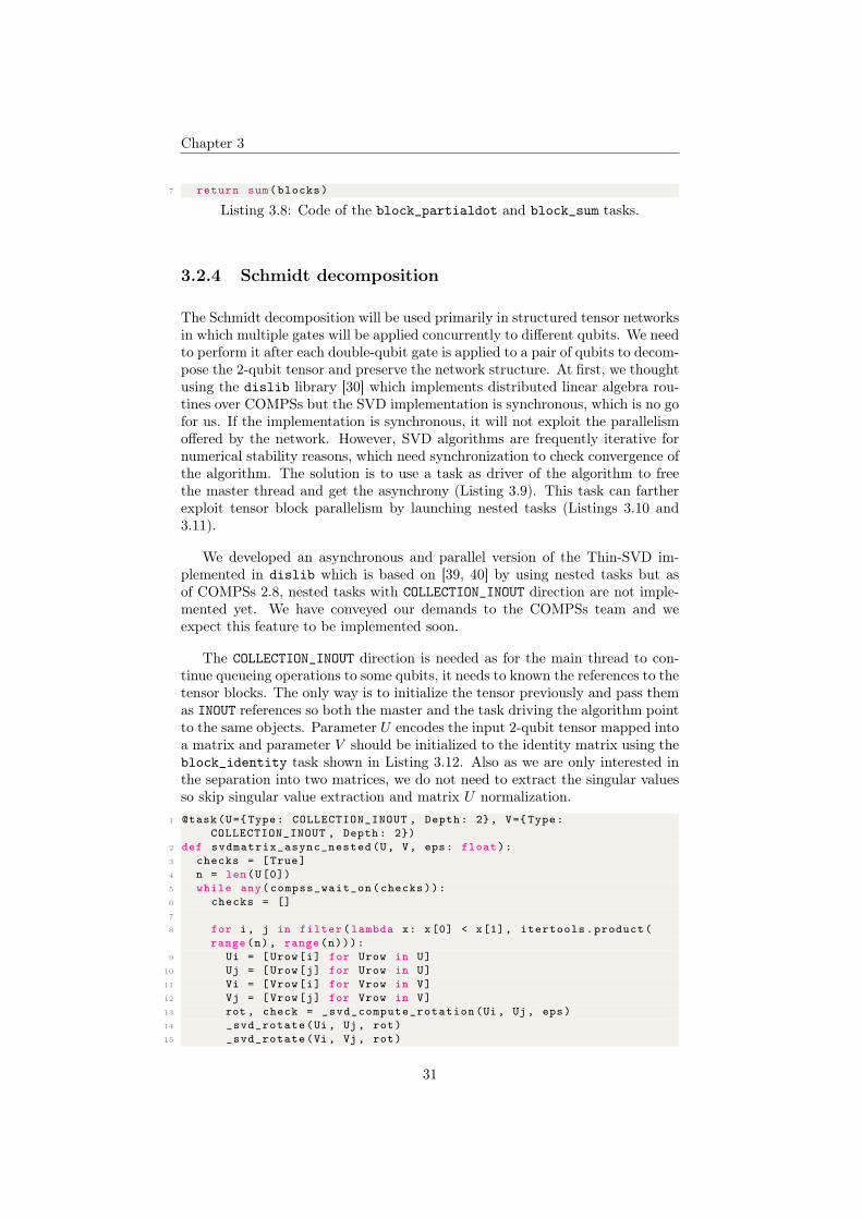
7 return sum(blocks)

Listing 3.8: Code of the block_partialdot and block_sum tasks.

3.2.4 Schmidt decomposition

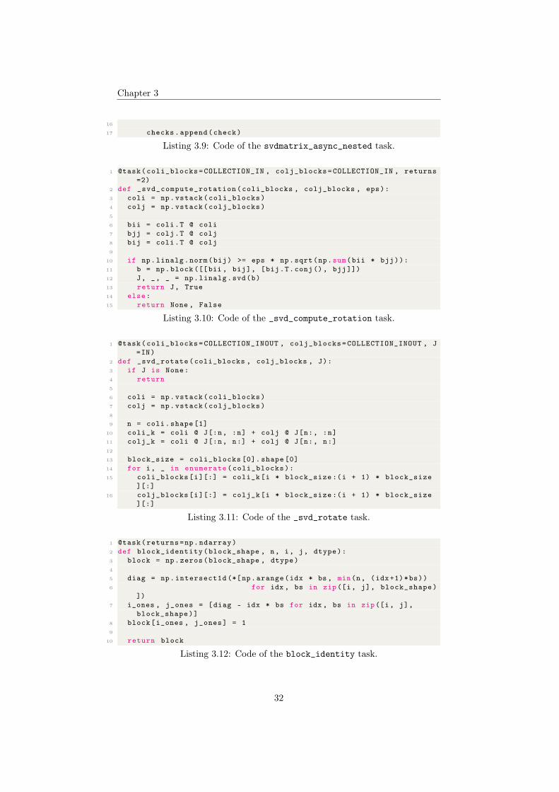
The Schmidt decomposition will be used primarily in structured tensor networksin which multiple gates will be applied concurrently to different qubits. We needto perform it after each double-qubit gate is applied to a pair of qubits to decom-pose the 2-qubit tensor and preserve the network structure. At first, we thoughtusing the dislib library [30] which implements distributed linear algebra rou-tines over COMPSs but the SVD implementation is synchronous, which is no gofor us. If the implementation is synchronous, it will not exploit the parallelismoffered by the network. However, SVD algorithms are frequently iterative fornumerical stability reasons, which need synchronization to check convergence ofthe algorithm. The solution is to use a task as driver of the algorithm to freethe master thread and get the asynchrony (Listing 3.9). This task can fartherexploit tensor block parallelism by launching nested tasks (Listings 3.10 and3.11).

We developed an asynchronous and parallel version of the Thin-SVD im-plemented in dislib which is based on [39, 40] by using nested tasks but asof COMPSs 2.8, nested tasks with COLLECTION_INOUT direction are not imple-mented yet. We have conveyed our demands to the COMPSs team and weexpect this feature to be implemented soon.

The COLLECTION_INOUT direction is needed as for the main thread to con-tinue queueing operations to some qubits, it needs to known the references to thetensor blocks. The only way is to initialize the tensor previously and pass themas INOUT references so both the master and the task driving the algorithm pointto the same objects. Parameter U encodes the input 2-qubit tensor mapped intoa matrix and parameter V should be initialized to the identity matrix using theblock_identity task shown in Listing 3.12. Also as we are only interested inthe separation into two matrices, we do not need to extract the singular valuesso skip singular value extraction and matrix U normalization.

1 @task(U={Type: COLLECTION_INOUT , Depth: 2}, V={Type:COLLECTION_INOUT , Depth: 2})

2 def svdmatrix_async_nested(U, V, eps: float):3 checks = [True]4 n = len(U[0])5 while any(compss_wait_on(checks)):6 checks = []7

8 for i, j in filter(lambda x: x[0] < x[1], itertools.product(range(n), range(n))):

9 Ui = [Urow[i] for Urow in U]10 Uj = [Urow[j] for Urow in U]11 Vi = [Vrow[i] for Vrow in V]12 Vj = [Vrow[j] for Vrow in V]13 rot , check = _svd_compute_rotation(Ui, Uj, eps)14 _svd_rotate(Ui, Uj, rot)15 _svd_rotate(Vi, Vj, rot)

31

Chapter 3

16

17 checks.append(check)

Listing 3.9: Code of the svdmatrix_async_nested task.

1 @task(coli_blocks=COLLECTION_IN , colj_blocks=COLLECTION_IN , returns=2)

2 def _svd_compute_rotation(coli_blocks , colj_blocks , eps):3 coli = np.vstack(coli_blocks)4 colj = np.vstack(colj_blocks)5

6 bii = coli.T @ coli7 bjj = colj.T @ colj8 bij = coli.T @ colj9

10 if np.linalg.norm(bij) >= eps * np.sqrt(np.sum(bii * bjj)):11 b = np.block ([[bii , bij], [bij.T.conj(), bjj]])12 J, _, _ = np.linalg.svd(b)13 return J, True14 else:15 return None , False

Listing 3.10: Code of the _svd_compute_rotation task.

1 @task(coli_blocks=COLLECTION_INOUT , colj_blocks=COLLECTION_INOUT , J=IN)

2 def _svd_rotate(coli_blocks , colj_blocks , J):3 if J is None:4 return5

6 coli = np.vstack(coli_blocks)7 colj = np.vstack(colj_blocks)8

9 n = coli.shape [1]10 coli_k = coli @ J[:n, :n] + colj @ J[n:, :n]11 colj_k = coli @ J[:n, n:] + colj @ J[n:, n:]12

13 block_size = coli_blocks [0]. shape [0]14 for i, _ in enumerate(coli_blocks):15 coli_blocks[i][:] = coli_k[i * block_size :(i + 1) * block_size

][:]16 colj_blocks[i][:] = colj_k[i * block_size :(i + 1) * block_size

][:]

Listing 3.11: Code of the _svd_rotate task.

1 @task(returns=np.ndarray)2 def block_identity(block_shape , n, i, j, dtype):3 block = np.zeros(block_shape , dtype)4

5 diag = np.intersect1d (*[np.arange(idx * bs, min(n, (idx+1)*bs))6 for idx , bs in zip([i, j], block_shape)

])7 i_ones , j_ones = [diag - idx * bs for idx , bs in zip([i, j],

block_shape)]8 block[i_ones , j_ones] = 19

10 return block

Listing 3.12: Code of the block_identity task.

32

Chapter 3

3.2.5 Rechunk

It has also been observed that this operation is not critical for our purposesso we chose to implement a naïve solution in which we iterate sequentiallyover each tensor index and decide whether it needs to be splitted, merged orremain unchanged. In this work, tensor indexes from our simulations havedimensionality 2 so the memory overhead of this processing will be at much ×2.

1 @task(blocks=COLLECTION_IN , returns=np.ndarray)2 def block_merge(blocks , axis: int):3 return np.stack(blocks , axis)

Listing 3.13: Code of the block_merge task.

1 @task(block=IN, returns ={Type: COLLECTION_OUT , Depth: 1})2 def block_split(block: np.ndarray , n: int , axis: int):3 return map(lambda x: x.copy(), np.split(block , n, axis))

Listing 3.14: Code of the block_split task.

3.2.6 Reshape

This task is used when we need to map a tensor into a matrix to perform alinear algebra operation, like the SVD, and then undo the mapping to get backa tensor.

1 @task(block=IN, returns=np.ndarray)2 def block_reshape(block: np.ndarray , shape: tuple):3 return block.reshape(shape , order=’F’)

Listing 3.15: Code of the block_reshape task.

3.3 Compatibility with the ecosystem

A significant proportion of the Python ecosystem for tensor networks is basedon the opt_einsum [12] library which provides an optimized version of numpy’seinsum function. Although its functionality has been partially merged intonumpy, it still counts with some extra features among which it is the capabilityof choosing the execution backend.

It offers Dask, PyTorch, Tensorflow, CuPy, Sparse, Theano, JAX and Auto-grad as native backends. However any user may craft its backend by implement-ing a standard API. First requirement of the API is to implement the tensordotand transpose functions with the interface as specified by numpy and must beavailable on the top module; e.g. if the library is called X, then it can accessthose functions by the X.tensordot and X.transpose names. A third functioneinsum is required for certain operations such as the trace or extraction of thediagonal for example. opt_einsum may also find certain contraction patternsthat can be efficiently executed with BLAS routines such as GEMV (matrix-vector product) or GEMM (matrix-matrix product) but it fallbacks to calling

33

Chapter 3

tensordot if einsum is not implemented. I have not implemented einsum aswe do not use such operations yet or we can rely on tensordot meanwhile, butI plan to support it in the future.

As we also implemented a class that acts on behalf of numpy’s ndarray, thisclass needs an accessible property attribute called shape that returns the sizeof each tensor index. After fulfilling these requirements, the library has beenverified to work with opt_einsum along as with quimb libraries just by addingthe backend=’X’ keyword argument to their respective contraction functions.But just setting the backend keyword will not benefit from tensor slicing.

In order to correctly use the library and slice tensors in blocks, we need firstto find the indexes to be sliced by using cotengra.SliceFinder. It supportsseveral parameters to customize the search, but in this work, we will only usethe target_size to limit the size of the largest tensor blocks. Then we computethe block_shape for each input tensor and finally replace each array of tensornetwork with a Tensor of our own. On construction of a Tensor, we passboth the array and block_shape, and it slices and uploads the subarrays to theCOMPSs runtime.

34

Chapter 4

Evaluation

In this chapter, we see the methods explained in previous chapters in action.Thanks to COMPSs’ integration with Extrae, our simulations can be traced andanalyzed performance-wise with Paraver [41]. We try to analyze the impact ofdifferent execution configurations in the execution time of the application andcheck if it can simulate a circuit whose resource requirements do not fit in onenode.

4.1 Infrastructure

On this work, we had access to the Marenostrum 4 supercomputer which isbased on Intel Xeon Platinum processors, Lenovo SD530 Compute Racks, aLinux Operating System and an Intel Omni-Path interconnection. It is thebiggest cluster of the Barcelona Supercomputing Center facilities.

• Peak performance of 11.15 PFLOP/s

• 3456 nodes:

– Intel Xeon Platinum 8160 24 cores @ 2.1 GHz ×2

– Hyperthreading off

• 384.75 TB of main memory

– 216 nodes with 12× 32 GB DDR4-2667 DIMMS (8 GB/core)– 3240 nodes with 12× 8 GB DDR4-2667 DIMMS (2 GB/core)

• Interconnection networks:

– 100 Gb Intel Omni-Path Full-Fat Tree– 10 Gb Ethernet

• Operating System: SUSE Linux Enterprise Server 12 SP2

35

Chapter 4

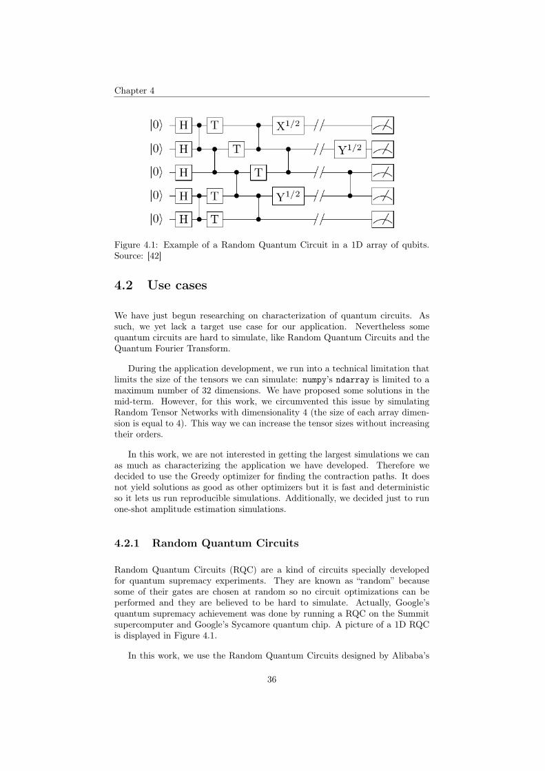
Figure 4.1: Example of a Random Quantum Circuit in a 1D array of qubits.Source: [42]

4.2 Use cases

We have just begun researching on characterization of quantum circuits. Assuch, we yet lack a target use case for our application. Nevertheless somequantum circuits are hard to simulate, like Random Quantum Circuits and theQuantum Fourier Transform.

During the application development, we run into a technical limitation thatlimits the size of the tensors we can simulate: numpy’s ndarray is limited to amaximum number of 32 dimensions. We have proposed some solutions in themid-term. However, for this work, we circumvented this issue by simulatingRandom Tensor Networks with dimensionality 4 (the size of each array dimen-sion is equal to 4). This way we can increase the tensor sizes without increasingtheir orders.

In this work, we are not interested in getting the largest simulations we canas much as characterizing the application we have developed. Therefore wedecided to use the Greedy optimizer for finding the contraction paths. It doesnot yield solutions as good as other optimizers but it is fast and deterministicso it lets us run reproducible simulations. Additionally, we decided just to runone-shot amplitude estimation simulations.

4.2.1 Random Quantum Circuits

Random Quantum Circuits (RQC) are a kind of circuits specially developedfor quantum supremacy experiments. They are known as “random” becausesome of their gates are chosen at random so no circuit optimizations can beperformed and they are believed to be hard to simulate. Actually, Google’squantum supremacy achievement was done by running a RQC on the Summitsupercomputer and Google’s Sycamore quantum chip. A picture of a 1D RQCis displayed in Figure 4.1.

In this work, we use the Random Quantum Circuits designed by Alibaba’s

36

Chapter 4

Figure 4.2: Histogram of input and intermediate tensors involved in the con-traction of the Alibaba’s Random Quantum Circuit with 53 qubits and depth10 using the Greedy optimizer.

Quantum team [43]. Due to the limitations with numpy explained earlier, we arejust able simulate a RQC of 53 qubits and depth 10. The RQCs with a higherdepth used in [43] yield intermediate tensor networks with a rank higher thanwhat numpy can handle, when using the Greedy optimizer.

4.2.2 Quantum Fourier Transform

The Quantum Fourier Trasform (QFT) is the quantum analogue of the DiscreteFourier Transform (DFT). It is an important component of many quantum algo-rithms such as Shor’s algorithm for integer factorization, which can theoreticallybe used for breaking current standard classical encryption protocols. A pictureof its circuit implementation is shown in Figure 1.2.

We noticed that n-qubit QFT exhibits an interesting pattern when using theGreedy optimizer to find the contraction pattern:

• The largest intermediate tensor has rank n if odd and n− 1 if even.• The number of arithmetic operations multiplies by nearly 8 every odd

number of qubits.

In Figure 4.3, we show the histogram of tensor sizes involved in the QFT

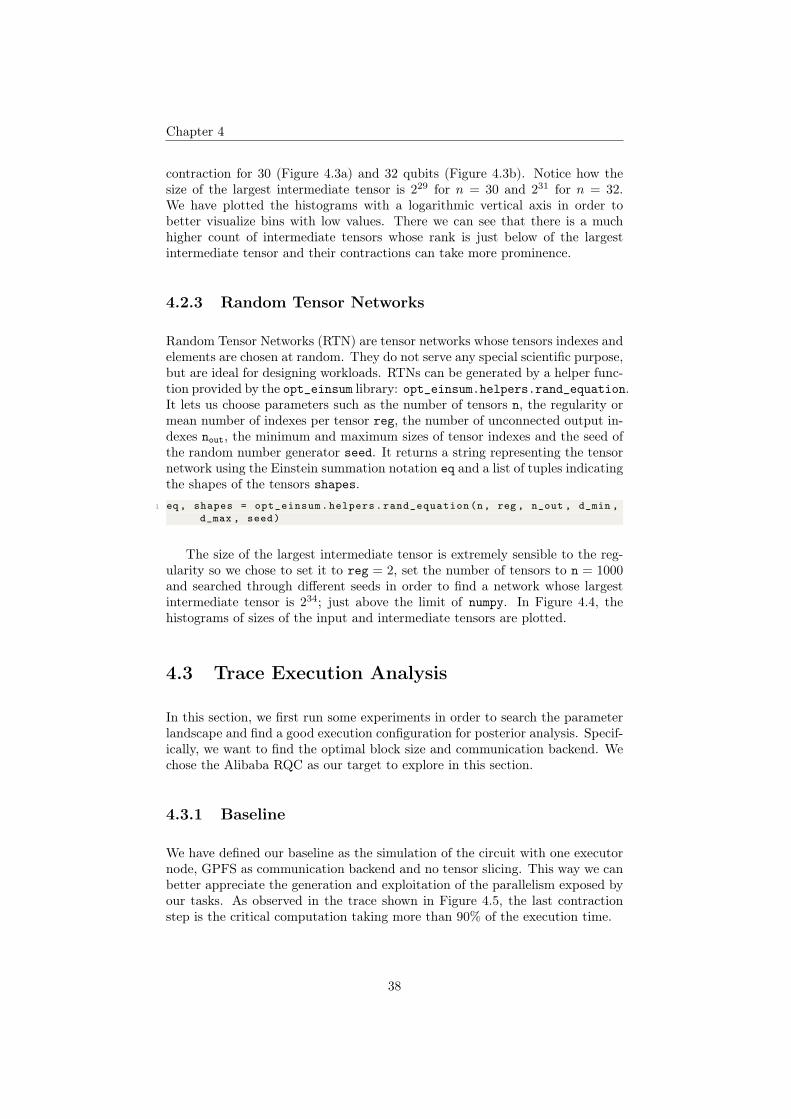
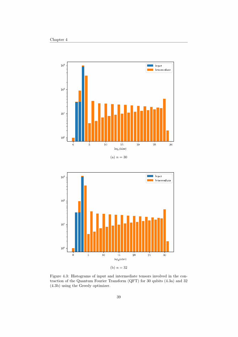
37

Chapter 4

contraction for 30 (Figure 4.3a) and 32 qubits (Figure 4.3b). Notice how thesize of the largest intermediate tensor is 229 for n = 30 and 231 for n = 32.We have plotted the histograms with a logarithmic vertical axis in order tobetter visualize bins with low values. There we can see that there is a muchhigher count of intermediate tensors whose rank is just below of the largestintermediate tensor and their contractions can take more prominence.

4.2.3 Random Tensor Networks

Random Tensor Networks (RTN) are tensor networks whose tensors indexes andelements are chosen at random. They do not serve any special scientific purpose,but are ideal for designing workloads. RTNs can be generated by a helper func-tion provided by the opt_einsum library: opt_einsum.helpers.rand_equation.It lets us choose parameters such as the number of tensors n, the regularity ormean number of indexes per tensor reg, the number of unconnected output in-dexes nout, the minimum and maximum sizes of tensor indexes and the seed ofthe random number generator seed. It returns a string representing the tensornetwork using the Einstein summation notation eq and a list of tuples indicatingthe shapes of the tensors shapes.

1 eq , shapes = opt_einsum.helpers.rand_equation(n, reg , n_out , d_min ,d_max , seed)

The size of the largest intermediate tensor is extremely sensible to the reg-ularity so we chose to set it to reg = 2, set the number of tensors to n = 1000and searched through different seeds in order to find a network whose largestintermediate tensor is 234; just above the limit of numpy. In Figure 4.4, thehistograms of sizes of the input and intermediate tensors are plotted.

4.3 Trace Execution Analysis

In this section, we first run some experiments in order to search the parameterlandscape and find a good execution configuration for posterior analysis. Specif-ically, we want to find the optimal block size and communication backend. Wechose the Alibaba RQC as our target to explore in this section.

4.3.1 Baseline

We have defined our baseline as the simulation of the circuit with one executornode, GPFS as communication backend and no tensor slicing. This way we canbetter appreciate the generation and exploitation of the parallelism exposed byour tasks. As observed in the trace shown in Figure 4.5, the last contractionstep is the critical computation taking more than 90% of the execution time.

38

Chapter 4

(a) n = 30

(b) n = 32

Figure 4.3: Histograms of input and intermediate tensors involved in the con-traction of the Quantum Fourier Transform (QFT) for 30 qubits (4.3a) and 32(4.3b) using the Greedy optimizer.

39

Chapter 4

Figure 4.4: Histograms of input and intermediate tensors involved in the con-traction of a Random Tensor Networks composed of 1000 tensors with regularity2 using the Greedy optimizer.

(a) COMPSs Tasks

(b) Events inside Tasks

Figure 4.5: Baseline trace for Alibaba RQC n = 53,m = 10 executed in 1 node.

40

Chapter 4

4.3.2 Experiment #1: Block Size

In this first experiment, we aim to find the effect of block size in the executionof the simulation. We decided to search a wide selection of block sizes from 220

to 228 elements.

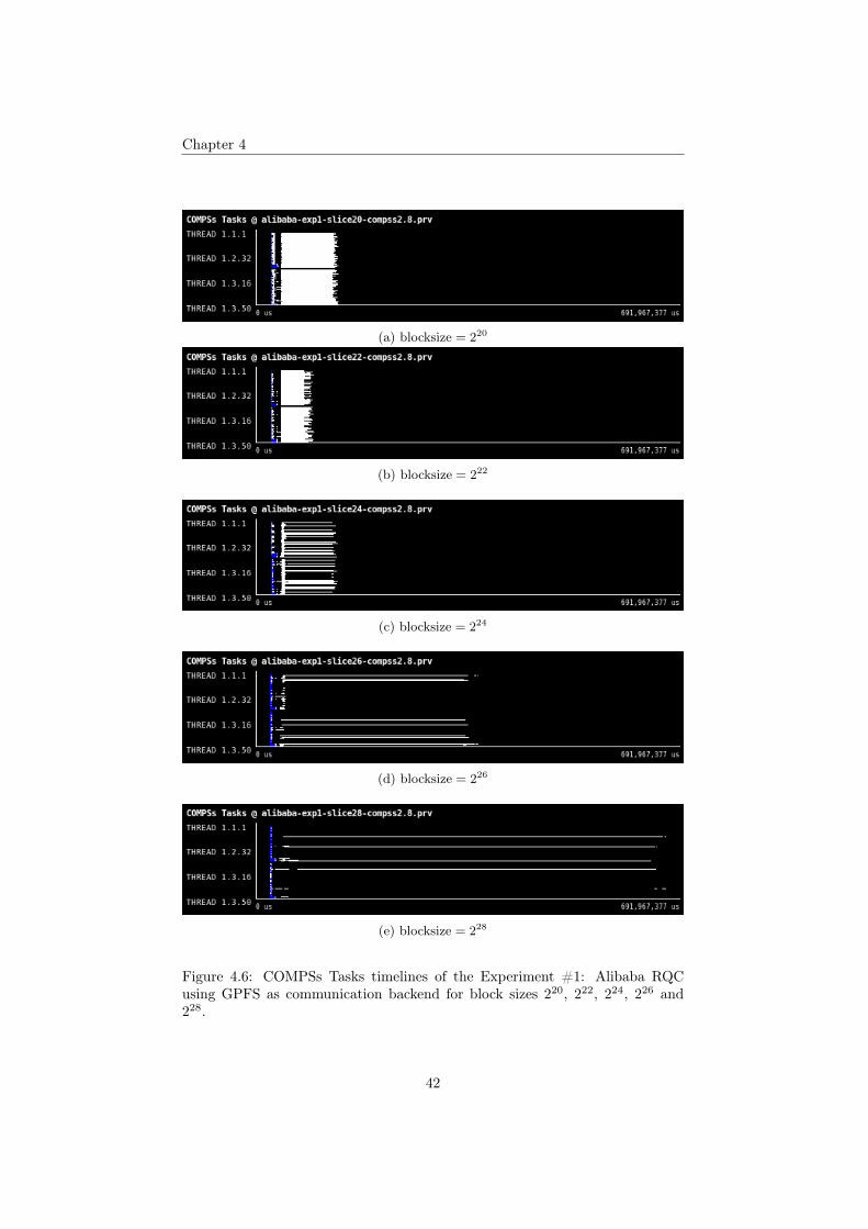
In Figure 4.6, we can see the timeline of executed tasks. First thing tonotice is that the block_pass takes practically no time and can be neglectedfrom the analysis. But just afterwards there is a blank space of between 5-8 s. Ifwe focus into the region, we appreciate that the subsequent block_tensordottasks look to be waiting to a couple of anomalous block_pass tasks that endureduring the whole blank space. This pattern repeats in all the traces that wehave analyzed. At first we thought it was because of the main thread tryingto upload a big tensor to COMPSs, but the block_pass task only takes placesat the beginning where tensors are minuscule (∼ 48 − 128 bytes). Our currenthypothesis is that there is some issue with the deserialization buffer but currentlywe lack the tools in order to explore this in depth. We expect the next versionof COMPSs to bring some light on this subject in the future as it will registerthe serialization and deserialization size of task objects, and task dependenciesby drawing communication lines inside the Paraver traces.

Continuing our analysis we see a clear tend on how as we grow the blocksize, the amount of parallel tasks decays exponentially and so does increase theexecution time of the dominating tasks associated to the largest intermediatetensor. In Figure 4.7, we have measured the parallel efficiency graph as the meannumber of simultaneously executing tasks. We can observer how efficiency peaksat 80% for a block size of 222 elements and then monotonically decreases, whichfits with the observations in Figure 4.6: As we grow the block size, tensor sliceshave a more coarsed granularity and the opportunities to exploit parallelismdiminish.

In Figure 4.8, we have plotted the “Events inside Tasks” timelines for thesame block size executions of Figure 4.6. This timeline shows the the time andinstants our application has devoted to user code (light green), deserialization(red) and serialization (dark green) of task data dependencies, import of librariesused in user code (red brownish), etcetera. The reader may appreciate that onthe first seconds of execution, the deserialization dominates the execution timeof tasks in the first contraction steps the tensors are too small in order tocompensate for communication. As the tensors grow larger on each contractionstep, block_tensordot tasks starts taking more time on user code and makeup for deserialization. But this may not happen as expected if block size is notbig enough as is seen in 4.8a where even though we obtain a high parallelismefficiency, the overhead of communication exceeds the user code time and thus,it decreases the performance of the application.

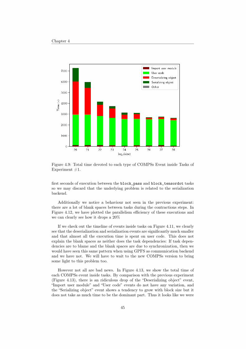
In Figure 4.9, we have plotted the total time of each event type extractedfrom Figure 4.8. We can clearly see that as we grow block size, user code remainsinvariant and serialization and deserialization of objects decreases quickly.

After watching these plots, we find that a block size of 222 is the optimal

41

Chapter 4

(a) blocksize = 220

(b) blocksize = 222

(c) blocksize = 224

(d) blocksize = 226

(e) blocksize = 228

Figure 4.6: COMPSs Tasks timelines of the Experiment #1: Alibaba RQCusing GPFS as communication backend for block sizes 220, 222, 224, 226 and228.

42

Chapter 4

Figure 4.7: Parallelism efficiency as the ratio of mean number of simultaneouslyexecuting tasks for Experiment #1.

configuration for this circuit as it has enough task to obtain a decent parallelismand tasks are not too fine grained for communication overhead to be dominant.Summarizing, a block size of 222 gets the best balance between parallelismefficiency and communication overhead for the Alibaba RQC circuit.

4.3.3 Experiment #2: Local serialization

As explained in Section 3.1, communication between tasks in COMPSs worksby serialization and deserialization of files. Depending of whether the filesys-tem of the working directory is mounted on a network or local, COMPSs mayperform differently. Network filesystems commonly work better when broadcastoperations are frequent while serialization to local disk and unicast distributiontends to shine when data reutilization by nodes is low.

We think that the latter can be similar to our case as tensors are only usedonce for contraction. We also changed to a Data Locality task scheduler so weminimize the amount of network communication. As we noticed in the previousexperiment that the amount of parallelism above a block size of 224 elements islow, we limited our traces to the range of block sizes between 220 and 224.

In Figure 4.10, we can see the timeline of executed tasks for this simulationconfiguration. As in the previous experiment, there is a blank space during the

43

Chapter 4

(a) blocksize = 220

(b) blocksize = 222

(c) blocksize = 224

(d) blocksize = 226

(e) blocksize = 228

Figure 4.8: Events inside Tasks timelines of the Experiment #1: Alibaba RQCusing GPFS as communication backend for block sizes 220, 222, 224, 226 and 228.

44

Chapter 4

Figure 4.9: Total time devoted to each type of COMPSs Event inside Tasks ofExperiment #1.

first seconds of execution between the block_pass and block_tensordot tasksso we may discard that the underlying problem is related to the serializationbackend.

Additionally we notice a behaviour not seen in the previous experiment:there are a lot of blank spaces between tasks during the contractions steps. InFigure 4.12, we have plotted the parallelism efficiency of these executions andwe can clearly see how it drops a 20%

If we check out the timeline of events inside tasks on Figure 4.11, we clearlysee that the deserialization and serialization events are significantly much smallerand that almost all the execution time is spent on user code. This does notexplain the blank spaces as neither does the task dependencies: If task depen-dencies are to blame and the blank spaces are due to synchronization, then wewould have seen this same pattern when using GPFS as communication backendand we have not. We will have to wait to the new COMPSs version to bringsome light to this problem too.

However not all are bad news. In Figure 4.13, we show the total time ofeach COMPSs event inside tasks. By comparison with the previous experiment(Figure 4.13), there is an ridiculous drop of the “Deserializing object” event,“Import user module” and “User code” events do not have any variation, andthe “Serializing object” event shows a tendency to grow with block size but itdoes not take as much time to be the dominant part. Thus it looks like we were

45

Chapter 4

(a) blocksize = 220

(b) blocksize = 221

(c) blocksize = 222

(d) blocksize = 223

(e) blocksize = 224

Figure 4.10: COMPSs Tasks timeline of the Alibaba RQC n = 53,m = 10simulation using local disk.

46

Chapter 4

(a) blocksize = 220

(b) blocksize = 221

(c) blocksize = 222

(d) blocksize = 223

(e) blocksize = 224

Figure 4.11: Events inside Tasks timeline of the Alibaba RQC n = 53,m = 10simulation using local disk.

47

Chapter 4

Figure 4.12: Parallelism efficiency of the Alibaba RQC n = 53,m = 10 simula-tion using local disk.

right on preferring unicast communication over broadcasting using a networkfilesystem, even though we run into the problem of blank spaces. Due to thisissue, we have decided to not use local disk as communication backend and useGPFS instead by default.

4.4 Scalability

In this section we aim to characterize our application’s scalability. Both strongand weak scalability are interesting for us. Weak scalability is a measure of thesize of the simulations we may run, and strong scalability gives us an intuitionon how good our application generates parallelization opportunities to keep thecores busy.

4.4.1 Strong Scalability

We have measured the strong scalability of our application by measuring thespeedup graphed for several configurations of the Alibaba RQC and QFT cir-cuits. The results are plotted in the graph of Figure 4.14. Some points are notshown due to erroneous execution.

48

Chapter 4

Figure 4.13: Total time devoted to each type of event inside tasks for the AlibabaRQC n = 53,m = 10 simulation using local disk.

Figure 4.14: Measured speedup for the Alibaba RQC and QFT simulations withdifferent execution configurations.

49

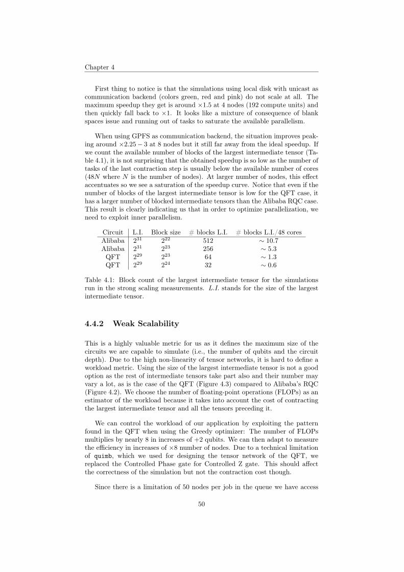
Chapter 4

First thing to notice is that the simulations using local disk with unicast ascommunication backend (colors green, red and pink) do not scale at all. Themaximum speedup they get is around ×1.5 at 4 nodes (192 compute units) andthen quickly fall back to ×1. It looks like a mixture of consequence of blankspaces issue and running out of tasks to saturate the available parallelism.

When using GPFS as communication backend, the situation improves peak-ing around ×2.25− 3 at 8 nodes but it still far away from the ideal speedup. Ifwe count the available number of blocks of the largest intermediate tensor (Ta-ble 4.1), it is not surprising that the obtained speedup is so low as the number oftasks of the last contraction step is usually below the available number of cores(48N where N is the number of nodes). At larger number of nodes, this effectaccentuates so we see a saturation of the speedup curve. Notice that even if thenumber of blocks of the largest intermediate tensor is low for the QFT case, ithas a larger number of blocked intermediate tensors than the Alibaba RQC case.This result is clearly indicating us that in order to optimize parallelization, weneed to exploit inner parallelism.

Circuit L.I. Block size # blocks L.I. # blocks L.I./48 coresAlibaba 231 222 512 ∼ 10.7Alibaba 231 223 256 ∼ 5.3QFT 229 223 64 ∼ 1.3QFT 229 224 32 ∼ 0.6

Table 4.1: Block count of the largest intermediate tensor for the simulationsrun in the strong scaling measurements. L.I. stands for the size of the largestintermediate tensor.

4.4.2 Weak Scalability

This is a highly valuable metric for us as it defines the maximum size of thecircuits we are capable to simulate (i.e., the number of qubits and the circuitdepth). Due to the high non-linearity of tensor networks, it is hard to define aworkload metric. Using the size of the largest intermediate tensor is not a goodoption as the rest of intermediate tensors take part also and their number mayvary a lot, as is the case of the QFT (Figure 4.3) compared to Alibaba’s RQC(Figure 4.2). We choose the number of floating-point operations (FLOPs) as anestimator of the workload because it takes into account the cost of contractingthe largest intermediate tensor and all the tensors preceding it.

We can control the workload of our application by exploiting the patternfound in the QFT when using the Greedy optimizer: The number of FLOPsmultiplies by nearly 8 in increases of +2 qubits. We can then adapt to measurethe efficiency in increases of ×8 number of nodes. Due to a technical limitationof quimb, which we used for designing the tensor network of the QFT, wereplaced the Controlled Phase gate for Controlled Z gate. This should affectthe correctness of the simulation but not the contraction cost though.

Since there is a limitation of 50 nodes per job in the queue we have access

50

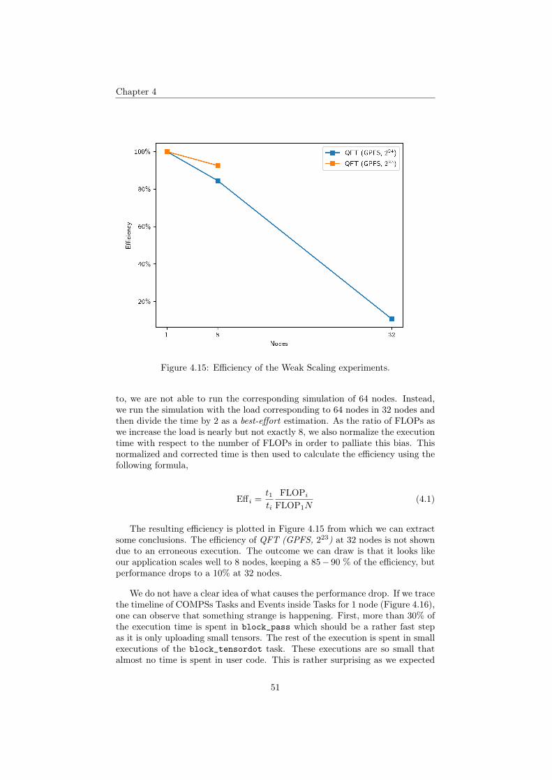
Chapter 4

Figure 4.15: Efficiency of the Weak Scaling experiments.

to, we are not able to run the corresponding simulation of 64 nodes. Instead,we run the simulation with the load corresponding to 64 nodes in 32 nodes andthen divide the time by 2 as a best-effort estimation. As the ratio of FLOPs aswe increase the load is nearly but not exactly 8, we also normalize the executiontime with respect to the number of FLOPs in order to palliate this bias. Thisnormalized and corrected time is then used to calculate the efficiency using thefollowing formula,

Effi =t1ti

FLOPiFLOP1N

(4.1)

The resulting efficiency is plotted in Figure 4.15 from which we can extractsome conclusions. The efficiency of QFT (GPFS, 223) at 32 nodes is not showndue to an erroneous execution. The outcome we can draw is that it looks likeour application scales well to 8 nodes, keeping a 85− 90 % of the efficiency, butperformance drops to a 10% at 32 nodes.

We do not have a clear idea of what causes the performance drop. If we tracethe timeline of COMPSs Tasks and Events inside Tasks for 1 node (Figure 4.16),one can observe that something strange is happening. First, more than 30% ofthe execution time is spent in block_pass which should be a rather fast stepas it is only uploading small tensors. The rest of the execution is spent in smallexecutions of the block_tensordot task. These executions are so small thatalmost no time is spent in user code. This is rather surprising as we expected

51

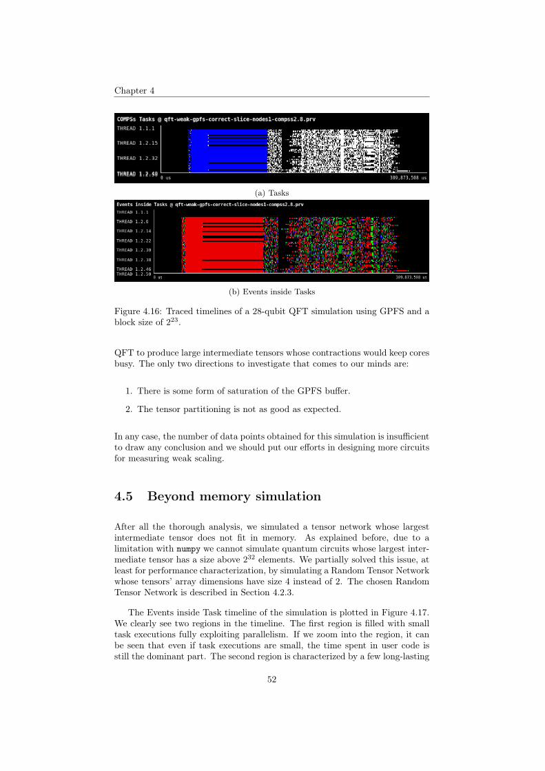
Chapter 4

(a) Tasks

(b) Events inside Tasks

Figure 4.16: Traced timelines of a 28-qubit QFT simulation using GPFS and ablock size of 223.

QFT to produce large intermediate tensors whose contractions would keep coresbusy. The only two directions to investigate that comes to our minds are:

1. There is some form of saturation of the GPFS buffer.

2. The tensor partitioning is not as good as expected.

In any case, the number of data points obtained for this simulation is insufficientto draw any conclusion and we should put our efforts in designing more circuitsfor measuring weak scaling.

4.5 Beyond memory simulation

After all the thorough analysis, we simulated a tensor network whose largestintermediate tensor does not fit in memory. As explained before, due to alimitation with numpy we cannot simulate quantum circuits whose largest inter-mediate tensor has a size above 232 elements. We partially solved this issue, atleast for performance characterization, by simulating a Random Tensor Networkwhose tensors’ array dimensions have size 4 instead of 2. The chosen RandomTensor Network is described in Section 4.2.3.

The Events inside Task timeline of the simulation is plotted in Figure 4.17.We clearly see two regions in the timeline. The first region is filled with smalltask executions fully exploiting parallelism. If we zoom into the region, it canbe seen that even if task executions are small, the time spent in user code isstill the dominant part. The second region is characterized by a few long-lasting

52

Chapter 4

task executions. This suggests that for big tensor networks the SliceFinderdoes not seem to yield an optimal partitioning.

(a) Original

(b) Zoom

Figure 4.17: Events inside Tasks timeline of a Random Tensor Network with1000 input tensors, regularity = 2, dimensionality size = 4, seed = 130, blocksize 222 (Largest intermediate: 234

53

Chapter 5

Conclusion

In this work, we have presented a general method for partitioning tensors intoblocks and developed algorithms for performing tensor algebra in such blockedlayout. Then, we implemented such algorithms using the task-based COMPSsprogramming model to attain parallel and distributed computation. Finally,we evaluated the achieved performance by our application and simulated somehard to simulate quantum circuits.

Although experiments showed that the application did not scale well forlarge number of nodes, we believe this is because of a mixture of parallelizationmisconfiguration, non-optimal partitioning scheme and lack of exploitation ofthe available inner parallelism that can be palliated. We are working closelywith the COMPSs team and we expect these problems to be solved soon.

Despite being a relative new topic, it has been surprising to discover thescarcity of solutions for distributed execution of tensor networks. The majorityof the publications we read had their code unavailable to the public and forthe ones whose code was open-sourced, documentation was scarce and theirapplications only worked for the case developed in their papers. We understandthat the problem is complex and that no general solution is found yet.

Even if there are some ideas on how to perform certain tensor operations ina distributed manner, there is no work unifying them and presenting them allalong with a proper characterization. We believe this work also sets a precedentin that direction by starting to unify ideas published in the wild.

The only general purpose open-sourced simulator we found is ExaTensorbut we could not make it work due to race conditions. Currently, ExaTensor isbeing rewritten from Fortran to C++ and is not production ready. It has alsobeen surprising to find technical limitations in certain standard libraries suchas numpy. The upper bound on the number of dimension of a ndarray seemsillogical to us and has severely limited our work.

In my opinion, the field offers a lot of potential and the presented solutions

54

Chapter 5

are still too poor so that quantum supremacy can be acclaimed.

5.1 Future Work

The application developed in this work is in its early stages of development andas such, many features or optimizations have not been tried yet due to technicallimitations and time constraints. In this section, we enumerate features andfixes that are planned to be integrated in the near-/mid-term.

5.1.1 Work around the numpy limit of 32 dimensions

This is our most critical technical limitation as of writing this work, as it upperbounds the order of the tensors we can build. Currently, we see three solutions:

• Wait for numpy maintainers to fix the issue.

• Make a wrapper around the ndarray class.

• Implement our own of the ndarray subclass.

Out of the three, the first would be ideal but it seems unlikely to be solvedsoon. The wrapper around ndarray is a dirty hack which may add maintenancecomplexity to the code and does not promise to scale well, and implementing ourown ndarray subclass is costly but gives us freedom to optimize our backends.The next steps are to analyze these options and decide which one convey us themost.

5.1.2 Develop a better slice finder

Although cotengra’s SliceFinder algorithm yields acceptable results, we thinkwe can do it better so we find optimal block and task granularity and schedul-ing sequences automatically by analyzing the contraction sequence returned byopt_einsum as a contraction tree. Luckily for us, the cotengra library exportsa ContractionTree class that wraps over the contraction sequence and pro-vides us extra information such as the tensor size and number of FLOPs at eachcontraction. Something similar was done in [43] in order to optimize certaincontraction patterns. If we use such information, we can turn the problem intoa task-assignment optimization problem for which we can find good solutionsefficiently.

55

Chapter 5

5.1.3 Implement an asynchronous and parallel version ofTruncated-SVD

Asynchronous execution of the Singular Decomposition is a must in order to sim-ulate Structured Tensor Networks, which are known for efficient representationof quantum states. As explained in Section 2.1.3, the Schmidt decomposition isperformed after a double-qubit tensor is applied between two connected tensors.As we apply more gates between the tensors, the dimensionality of the tensor in-dex connecting both tensors will grow exponentially fast. In order to limit theirsize, rank-k approximations are performed rather than exact decompositions.

5.1.4 Offload costly linear algebra operations to GPUs

To make GPUs worth using them, the computation complexity of a kernel shouldbe higher than the communication complexity (the cost of sending the datathrough the bus). There are some tensor operations that adjust to this prop-erty; specifically tensor contraction and the Schmidt decomposition. Thanks toCOMPSs capability of multiple task implementations and the seamless integra-tion of CUDA with numpy through cupy, we foresee a working heterogeneoussystem in which the scheduler eases the burden of selecting the executor.

5.1.5 Integrate with optimized tensor transpositions li-braries

Optimal tensor permutation is not a trivial problem. Luckily for us, severallibraries have been published in the last years [32, 33, 34]. We would like totest and integrate them into our application to speedup the tensor permutationoperation.

5.1.6 Integrate with TBLIS

In [44], the author presents a method for tensor contraction without the need oftransposing them into matrices and develops a library based on linear algebrakernels extracted from the BLIS library. We would like to try it as such methodwould significantly decrease our computation time.

56

Bibliography

[1] F. Arute, K. Arya, R. Babbush, D. Bacon, J. C. Bardin, R. Barends,R. Biswas, S. Boixo, F. G. S. L. Brandao, D. A. Buell, B. Burkett, Y. Chen,Z. Chen, B. Chiaro, R. Collins, W. Courtney, A. Dunsworth, E. Farhi,B. Foxen, A. Fowler, C. Gidney, M. Giustina, R. Graff, K. Guerin, S. Habeg-ger, M. P. Harrigan, M. J. Hartmann, A. Ho, M. Hoffmann, T. Huang,T. S. Humble, S. V. Isakov, E. Jeffrey, Z. Jiang, D. Kafri, K. Kechedzhi,J. Kelly, P. V. Klimov, S. Knysh, A. Korotkov, F. Kostritsa, D. Land-huis, M. Lindmark, E. Lucero, D. Lyakh, S. Mandrà, J. R. McClean,M. McEwen, A. Megrant, X. Mi, K. Michielsen, M. Mohseni, J. Mutus,O. Naaman, M. Neeley, C. Neill, M. Y. Niu, E. Ostby, A. Petukhov, J. C.Platt, C. Quintana, E. G. Rieffel, P. Roushan, N. C. Rubin, D. Sank, K. J.Satzinger, V. Smelyanskiy, K. J. Sung, M. D. Trevithick, A. Vainsencher,B. Villalonga, T. White, Z. J. Yao, P. Yeh, A. Zalcman, H. Neven, andJ. M. Martinis, “Quantum supremacy using a programmable superconduct-ing processor,” Nature, vol. 574, pp. 505–510, Oct. 2019.

[2] M. A. Nielsen and I. L. Chuang, Quantum computation and quantum in-formation. Cambridge ; New York: Cambridge University Press, 10thanniversary ed ed., 2010.

[3] T. Jones, A. Brown, I. Bush, and S. C. Benjamin, “QuEST and High Per-formance Simulation of Quantum Computers,” Scientific Reports, vol. 9,p. 10736, Dec. 2019.

[4] S. Boixo, S. V. Isakov, V. N. Smelyanskiy, and H. Neven, “Simulationof low-depth quantum circuits as complex undirected graphical models,”arXiv:1712.05384 [quant-ph], Jan. 2018. arXiv: 1712.05384.

[5] I. L. Markov, A. Fatima, S. V. Isakov, and S. Boixo, “Quantum SupremacyIs Both Closer and Farther than It Appears,” arXiv:1807.10749 [quant-ph],Sept. 2018. arXiv: 1807.10749.

[6] Bradley, Tai-Danae, “Matrices as Tensor Network Diagrams.” https://www.math3ma.com/blog/matrices-as-tensor-network-diagrams.

[7] J. Biamonte, “On the Theory of Modern Quantum Algorithms,”arXiv:2009.10088 [math-ph, physics:quant-ph], Sept. 2020. arXiv:2009.10088.

57

Chapter 5

[8] R. Orus, “A Practical Introduction to Tensor Networks: Matrix ProductStates and Projected Entangled Pair States,” Annals of Physics, vol. 349,pp. 117–158, Oct. 2014. arXiv: 1306.2164.

[9] R. Orus, “Tensor networks for complex quantum systems,” Nature ReviewsPhysics, vol. 1, pp. 538–550, Sept. 2019. tex.ids: orus_tensor_2019-1arXiv: 1812.04011.

[10] S.-J. Ran, E. Tirrito, C. Peng, X. Chen, L. Tagliacozzo, G. Su,and M. Lewenstein, “Lecture Notes of Tensor Network Contractions,”arXiv:1708.09213 [cond-mat, physics:physics, physics:quant-ph], vol. 964,2020. arXiv: 1708.09213.

[11] J. C. Bridgeman and C. T. Chubb, “Hand-waving and interpretive dance:an introductory course on tensor networks,” J. Phys. A, p. 62, 2017. tex.ids:bridgeman_hand-waving_2017-1.

[12] D. G. A. Smith and J. Gray, “opt_einsum - A Python package for optimiz-ing contraction order for einsum-like expressions,” Journal of Open SourceSoftware, vol. 3, p. 753, June 2018.

[13] J. Gray and S. Kourtis, “Hyper-optimized tensor network contraction,”Quantum, vol. 5, p. 410, Mar. 2021.

[14] Y. Zhou, E. M. Stoudenmire, and X. Waintal, “What limits the simulationof quantum computers?,” arXiv:2002.07730 [cond-mat, physics:quant-ph],Mar. 2020. arXiv: 2002.07730.

[15] “Tensor Network.” https://tensornetwork.org/. Accessed on: 2020-07-27.

[16] M. Smelyanskiy, N. P. D. Sawaya, and A. Aspuru-Guzik, “qHiP-STER: The Quantum High Performance Software Testing Environment,”arXiv:1601.07195 [quant-ph], May 2016. arXiv: 1601.07195.

[17] D. S. Steiger, T. Häner, and M. Troyer, “ProjectQ: An Open Source Soft-ware Framework for Quantum Computing,” Quantum, vol. 2, p. 49, Jan.2018. arXiv: 1612.08091.

[18] V. Gheorghiu, “Quantum++: A modern C++ quantum computing li-brary,” PLOS ONE, vol. 13, p. e0208073, Dec. 2018.

[19] H. De Raedt, F. Jin, D. Willsch, M. Willsch, N. Yoshioka, N. Ito, S. Yuan,and K. Michielsen, “Massively parallel quantum computer simulator, elevenyears later,” Computer Physics Communications, vol. 237, pp. 47–61, Apr.2019.

[20] S. Efthymiou, S. Ramos-Calderer, C. Bravo-Prieto, A. Pérez-Salinas,D. García-Martín, A. Garcia-Saez, J. I. Latorre, and S. Carrazza,“Qibo: a framework for quantum simulation with hardware acceleration,”arXiv:2009.01845 [quant-ph], Sept. 2020. arXiv: 2009.01845.

[21] G. G. Guerreschi, J. Hogaboam, F. Baruffa, and N. P. D. Sawaya, “IntelQuantum Simulator: A cloud-ready high-performance simulator of quan-tum circuits,” Quantum Science and Technology, vol. 5, p. 034007, May2020. arXiv: 2001.10554.

58

Chapter 5

[22] I. L. Markov and Y. Shi, “Simulating quantum computation by contract-ing tensor networks,” arXiv:quant-ph/0511069, July 2009. arXiv: quant-ph/0511069.

[23] D. Lyakh, “ExaTENSOR,” 2019.

[24] B. Villalonga, S. Boixo, B. Nelson, C. Henze, E. Rieffel, R. Biswas, andS. Mandrà, “A flexible high-performance simulator for verifying and bench-marking quantum circuits implemented on real hardware,” npj QuantumInformation, vol. 5, p. 86, Dec. 2019. arXiv: 1811.09599.

[25] B. Villalonga, D. Lyakh, S. Boixo, H. Neven, T. S. Humble, R. Biswas,E. G. Rieffel, A. Ho, and S. Mandrà, “Establishing the Quantum SupremacyFrontier with a 281 Pflop/s Simulation,” Quantum Science and Technology,vol. 5, p. 034003, Apr. 2020. arXiv: 1905.00444.

[26] E. Pednault, J. A. Gunnels, G. Nannicini, L. Horesh, T. Magerlein,E. Solomonik, E. W. Draeger, E. T. Holland, and R. Wisnieff, “Pareto-Efficient Quantum Circuit Simulation Using Tensor Contraction Deferral,”arXiv:1710.05867 [quant-ph], Aug. 2020. arXiv: 1710.05867.

[27] T. Nguyen, D. Lyakh, E. Dumitrescu, D. Clark, J. Larkin, and A. Mc-Caskey, “Tensor Network Quantum Virtual Machine for Simulating Quan-tum Circuits at Exascale,” arXiv:2104.10523 [quant-ph], Apr. 2021. arXiv:2104.10523.

[28] E. Solomonik, D. Matthews, J. R. Hammond, and J. Demmel, “CyclopsTensor Framework: reducing communication and eliminating load imbal-ance in massively parallel contractions,” p. 13.

[29] J. Gray, “quimb: A python package for quantum information and many-body calculations,” Journal of Open Source Software, vol. 3, p. 819, Sept.2018.

[30] J. Alvarez Cid-Fuentes, S. Sola, P. Alvarez, A. Castro-Ginard, and R. M.Badia, “dislib: Large Scale High Performance Machine Learning in Python,”in 2019 15th International Conference on eScience (eScience), (San Diego,CA, USA), pp. 96–105, IEEE, Sept. 2019.

[31] D. I. Lyakh, “Domain-specific virtual processors as a portable program-ming and execution model for parallel computational workloads on modernheterogeneous high-performance computing architectures,” InternationalJournal of Quantum Chemistry, vol. 119, p. e25926, June 2019.

[32] D. I. Lyakh, “An efficient tensor transpose algorithm for multicore CPU,Intel Xeon Phi, and NVidia Tesla GPU,” Computer Physics Communica-tions, vol. 189, pp. 84–91, Apr. 2015.

[33] P. Springer, T. Su, and P. Bientinesi, “HPTT: A High-Performance TensorTransposition C++ Library,” arXiv:1704.04374 [cs], May 2017. arXiv:1704.04374.

[34] A.-P. Hynninen and D. I. Lyakh, “cuTT: A High-Performance TensorTranspose Library for CUDA Compatible GPUs,” arXiv:1705.01598 [cs],May 2017. arXiv: 1705.01598.

59

Chapter 5

[35] R. M. Badia, J. Conejero, C. Diaz, J. Ejarque, D. Lezzi, F. Lordan,C. Ramon-Cortes, and R. Sirvent, “COMP Superscalar, an interoperableprogramming framework,” SoftwareX, vol. 3-4, pp. 32–36, Dec. 2015.

[36] F. Lordan, E. Tejedor, J. Ejarque, and R. Rafanell, “ServiceSs: an inter-operable programming framework for the Cloud,” p. 20.

[37] E. Tejedor, Y. Becerra, G. Alomar, A. Queralt, R. M. Badia, J. Torres,T. Cortes, and J. Labarta, “PyCOMPSs: Parallel computational workflowsin Python,” The International Journal of High Performance ComputingApplications, vol. 31, pp. 66–82, Jan. 2017.

[38] C. R. Harris, K. J. Millman, S. J. van der Walt, R. Gommers, P. Virta-nen, D. Cournapeau, E. Wieser, J. Taylor, S. Berg, N. J. Smith, R. Kern,M. Picus, S. Hoyer, M. H. van Kerkwijk, M. Brett, A. Haldane, J. F. delRío, M. Wiebe, P. Peterson, P. Gérard-Marchant, K. Sheppard, T. Reddy,W. Weckesser, H. Abbasi, C. Gohlke, and T. E. Oliphant, “Array program-ming with NumPy,” Nature, vol. 585, pp. 357–362, Sept. 2020.

[39] J. Dongarra, M. Gates, A. Haidar, J. Kurzak, P. Luszczek, S. Tomov, andI. Yamazaki, “The Singular Value Decomposition: Anatomy of Optimizingan Algorithm for Extreme Scale,” SIAM Review, vol. 60, pp. 808–865, Jan.2018.

[40] P. Arbenz and I. Slapnicar, “An Analysis of Parallel Implementations ofthe Block-Jacobi Algorithm for Computing the SVD,” p. 6.

[41] V. Pillet, J. Labarta, T. Cortes, and S. Girona, “Paraver: A tool to visualizeand analyze parallel code,” in Proceedings of WoTUG-18: transputer andoccam developments, vol. 44, pp. 17–31, Citeseer, 1995.

[42] S. Boixo, S. V. Isakov, V. N. Smelyanskiy, R. Babbush, N. Ding, Z. Jiang,M. J. Bremner, J. M. Martinis, and H. Neven, “Characterizing QuantumSupremacy in Near-Term Devices,” Nature Physics, vol. 14, pp. 595–600,June 2018. arXiv: 1608.00263.

[43] C. Huang, F. Zhang, M. Newman, J. Cai, X. Gao, Z. Tian, J. Wu, H. Xu,H. Yu, B. Yuan, M. Szegedy, Y. Shi, and J. Chen, “Classical Simulationof Quantum Supremacy Circuits,” arXiv:2005.06787 [quant-ph], May 2020.arXiv: 2005.06787.

[44] D. A. Matthews, “High-Performance Tensor Contraction without Transpo-sition,” arXiv:1607.00291 [cs], July 2017. arXiv: 1607.00291.

60

List of Figures

1.1 Photograph of Google’s Sycamore quantum chip based on super-conducting technology . . . . . . . . . . . . . . . . . . . . . . . . 6

1.2 Circuit representing the Quantum Fourier Transform . . . . . . . 9

1.3 Illustration of the partition schemes used to distribute the statevector . . . . . . . . . . . . . . . . . . . . . . . . . . . . . . . . . 10

1.4 Cheatsheet diagrams of low-order tensor representations . . . . . 12

1.5 Tensor network diagram of Equation 1.13. . . . . . . . . . . . . . 13

1.6 Popular structured tensor networks. Source: [15] . . . . . . . . . 14

2.1 Hyperrectangle of a tensor block defined by vectors b and e. . . . 18

2.2 Tensor sliced into an uniform grid of blocks . . . . . . . . . . . . 18

2.3 Diagram of the tensor permutation operation. . . . . . . . . . . . 19

2.4 Mapping from 3-order tensor to matrix . . . . . . . . . . . . . . . 21

2.5 Steps of Tensor Contraction using Dimension Extents . . . . . . 22

2.6 Tensor cutting or slicing example. Source: [13] . . . . . . . . . . 24

4.1 Example of a Random Quantum Circuit in a 1D array of qubits.Source: [42] . . . . . . . . . . . . . . . . . . . . . . . . . . . . . . 36

4.2 Histogram of input and intermediate tensors involved in the con-traction of the Alibaba’s Random Quantum Circuit with 53 qubitsand depth 10 using the Greedy optimizer. . . . . . . . . . . . . . 37

4.3 Histograms of input and intermediate tensors involved in the con-traction of the Quantum Fourier Transform (QFT) for 30 qubits(4.3a) and 32 (4.3b) using the Greedy optimizer. . . . . . . . . . 39

4.4 Histograms of input and intermediate tensors involved in the con-traction of a Random Tensor Networks composed of 1000 tensorswith regularity 2 using the Greedy optimizer. . . . . . . . . . . . 40

4.5 Baseline trace for Alibaba RQC n = 53,m = 10 executed in 1node. . . . . . . . . . . . . . . . . . . . . . . . . . . . . . . . . . . 40

61

Chapter 5

4.6 COMPSs Tasks timelines of the Experiment #1: Alibaba RQCusing GPFS as communication backend for block sizes 220, 222,224, 226 and 228. . . . . . . . . . . . . . . . . . . . . . . . . . . . 42

4.7 Parallelism efficiency as the ratio of mean number of simultane-ously executing tasks for Experiment #1. . . . . . . . . . . . . . 43

4.8 Events inside Tasks timelines of the Experiment #1: AlibabaRQC using GPFS as communication backend for block sizes 220,222, 224, 226 and 228. . . . . . . . . . . . . . . . . . . . . . . . . . 44

4.9 Total time devoted to each type of COMPSs Event inside Tasksof Experiment #1. . . . . . . . . . . . . . . . . . . . . . . . . . . 45

4.10 COMPSs Tasks timeline of the Alibaba RQC n = 53,m = 10simulation using local disk. . . . . . . . . . . . . . . . . . . . . . 46

4.11 Events inside Tasks timeline of the Alibaba RQC n = 53,m = 10simulation using local disk. . . . . . . . . . . . . . . . . . . . . . 47

4.12 Parallelism efficiency of the Alibaba RQC n = 53,m = 10 simu-lation using local disk. . . . . . . . . . . . . . . . . . . . . . . . . 48

4.13 Total time devoted to each type of event inside tasks for theAlibaba RQC n = 53,m = 10 simulation using local disk. . . . . 49

4.14 Measured speedup for the Alibaba RQC and QFT simulationswith different execution configurations. . . . . . . . . . . . . . . . 49

4.15 Efficiency of the Weak Scaling experiments. . . . . . . . . . . . . 51

4.16 Traced timelines of a 28-qubit QFT simulation using GPFS anda block size of 223. . . . . . . . . . . . . . . . . . . . . . . . . . . 52

4.17 Events inside Tasks timeline of a Random Tensor Network with1000 input tensors, regularity = 2, dimensionality size = 4, seed= 130, block size 222 (Largest intermediate: 234 . . . . . . . . . . 53

62

List of Tables

2.1 Example of computing the grid or block_shape for a given ten-sor contraction. . . . . . . . . . . . . . . . . . . . . . . . . . . . . 21

4.1 Block count of the largest intermediate tensor for the simulationsrun in the strong scaling measurements . . . . . . . . . . . . . . 50

63