Quantum Computing Summer School - ERA
332
Quantum Computing Summer School [Home] [Members] [Schedule] [Overview] [Sponsors] [Archive/Links] [Contact] Home | Members | Schedule | Overview | Sponsors | Archive/Links | Contact Copyright (C) by V.Bulitko, 2000-2002. All Rights Reserved. For problems or questions regarding this web contact V.Bulitko. Last updated: 03/08/02. http://www.cs.ualberta.ca/~bulitko/qc/ [6/27/2002 2:41:32 PM]
-
Upload
khangminh22 -
Category
Documents
-
view
0 -
download
0
Transcript of Quantum Computing Summer School - ERA
Quantum Computing Summer School
[Home][Members][Schedule][Overview][Sponsors][Archive/Links][Contact]
Home | Members | Schedule | Overview | Sponsors | Archive/Links | Contact
Copyright (C) by V.Bulitko, 2000-2002. All Rights Reserved.For problems or questions regarding this web contact V.Bulitko.
Last updated: 03/08/02.
http://www.cs.ualberta.ca/~bulitko/qc/ [6/27/2002 2:41:32 PM]
Members
[Home][Members][Schedule][Overview][Sponsors][Archive/Links][Contact]
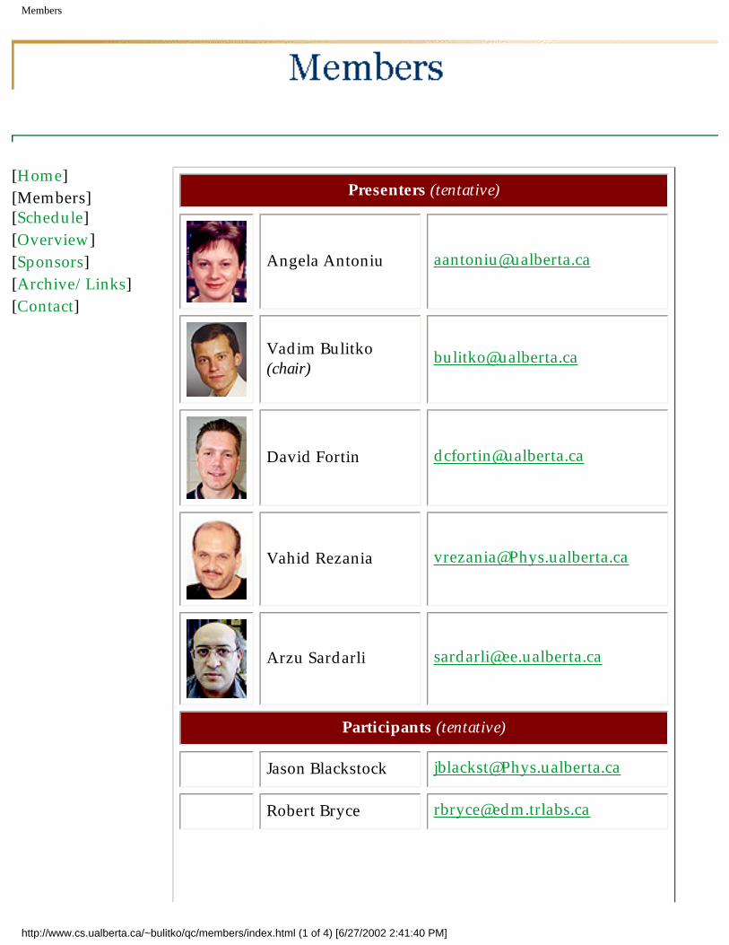
Presenters (tentative)
Angela Antoniu [email protected]
Vadim Bulitko(chair)
David Fortin [email protected]
Vahid Rezania [email protected]
Arzu Sardarli [email protected]
Participants (tentative)
Jason Blackstock [email protected]
Robert Bryce [email protected]
http://www.cs.ualberta.ca/~bulitko/qc/members/index.html (1 of 4) [6/27/2002 2:41:40 PM]
Members
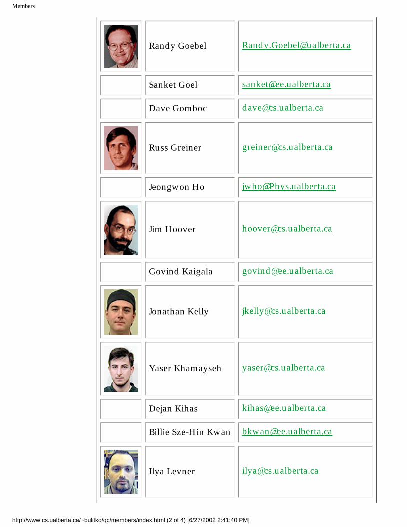
Randy Goebel [email protected]
Sanket Goel [email protected]
Dave Gomboc [email protected]
Russ Greiner [email protected]
Jeongwon Ho [email protected]
Jim Hoover [email protected]
Govind Kaigala [email protected]
Jonathan Kelly [email protected]
Yaser Khamayseh [email protected]
Dejan Kihas [email protected]
Billie Sze-Hin Kwan [email protected]
Ilya Levner [email protected]
http://www.cs.ualberta.ca/~bulitko/qc/members/index.html (2 of 4) [6/27/2002 2:41:40 PM]
Members
Peter Xiaoping Liu [email protected]
Omid Madani [email protected]
Bruce Matichuk [email protected]
Samer Nassar [email protected]
Jim Nastos [email protected]
Ashikur Rahman [email protected]
Lino Ramirez [email protected]
Marlene Rodriguez [email protected]
Daniel Salamon [email protected]
Ajit Paul Singh [email protected]
Dan Tzur [email protected]
Eric Woolgar [email protected]
http://www.cs.ualberta.ca/~bulitko/qc/members/index.html (3 of 4) [6/27/2002 2:41:40 PM]

Members
Herb Yang [email protected]
Peter Yap [email protected]
Home | Members | Schedule | Overview | Sponsors | Archive/Links | Contact
Copyright (C) by V.Bulitko, 2000-2002. All Rights Reserved.For problems or questions regarding this web contact V.Bulitko.
Last updated: 03/08/02.
http://www.cs.ualberta.ca/~bulitko/qc/members/index.html (4 of 4) [6/27/2002 2:41:40 PM]
Schedule
[Home][Members][Schedule][Overview][Sponsors][Archive/Links][Contact]
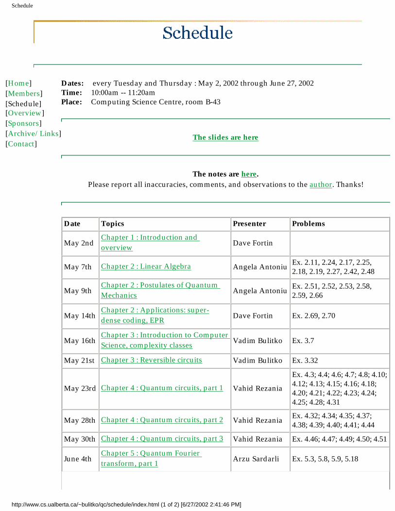
Dates: every Tuesday and Thursday : May 2, 2002 through June 27, 2002Time: 10:00am -- 11:20amPlace: Computing Science Centre, room B-43
The slides are here
The notes are here. Please report all inaccuracies, comments, and observations to the author. Thanks!
Date Topics Presenter Problems
May 2ndChapter 1 : Introduction and overview Dave Fortin
May 7th Chapter 2 : Linear Algebra Angela Antoniu Ex. 2.11, 2.24, 2.17, 2.25, 2.18, 2.19, 2.27, 2.42, 2.48
May 9thChapter 2 : Postulates of Quantum Mechanics Angela Antoniu Ex. 2.51, 2.52, 2.53, 2.58,
2.59, 2.66
May 14thChapter 2 : Applications: super-dense coding, EPR Dave Fortin Ex. 2.69, 2.70
May 16thChapter 3 : Introduction to Computer Science, complexity classes Vadim Bulitko Ex. 3.7
May 21st Chapter 3 : Reversible circuits Vadim Bulitko Ex. 3.32
May 23rd Chapter 4 : Quantum circuits, part 1 Vahid Rezania
Ex. 4.3; 4.4; 4.6; 4.7; 4.8; 4.10; 4.12; 4.13; 4.15; 4.16; 4.18; 4.20; 4.21; 4.22; 4.23; 4.24; 4.25; 4.28; 4.31
May 28th Chapter 4 : Quantum circuits, part 2 Vahid Rezania Ex. 4.32; 4.34; 4.35; 4.37; 4.38; 4.39; 4.40; 4.41; 4.44
May 30th Chapter 4 : Quantum circuits, part 3 Vahid Rezania Ex. 4.46; 4.47; 4.49; 4.50; 4.51
June 4thChapter 5 : Quantum Fourier transform, part 1 Arzu Sardarli Ex. 5.3, 5.8, 5.9, 5.18
http://www.cs.ualberta.ca/~bulitko/qc/schedule/index.html (1 of 2) [6/27/2002 2:41:46 PM]
Schedule
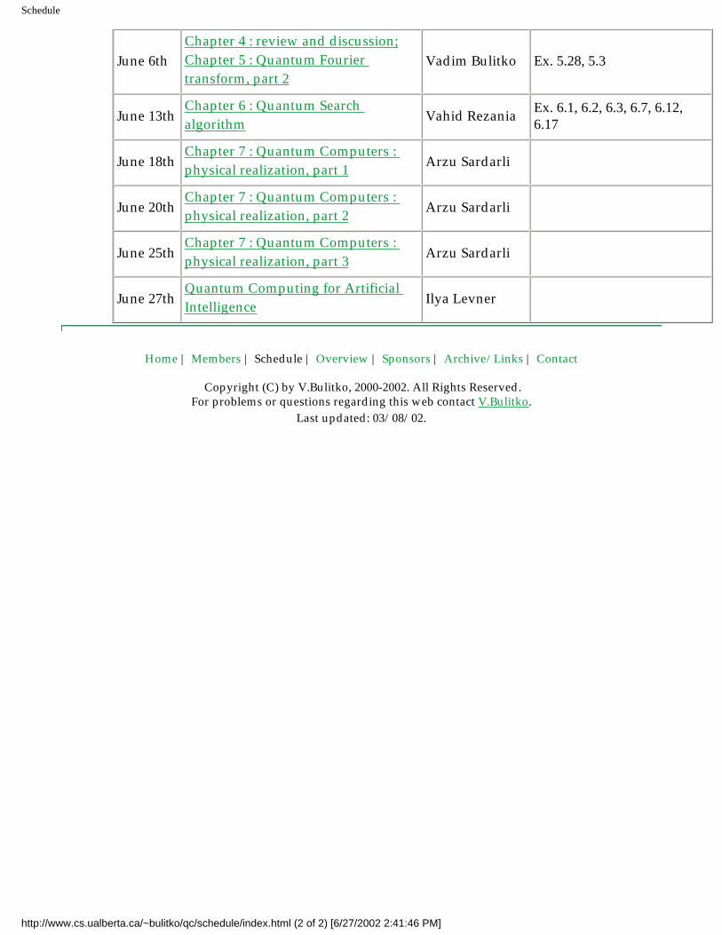
June 6thChapter 4 : review and discussion;Chapter 5 : Quantum Fourier transform, part 2
Vadim Bulitko Ex. 5.28, 5.3
June 13thChapter 6 : Quantum Search algorithm Vahid Rezania Ex. 6.1, 6.2, 6.3, 6.7, 6.12,
6.17
June 18thChapter 7 : Quantum Computers : physical realization, part 1 Arzu Sardarli
June 20thChapter 7 : Quantum Computers : physical realization, part 2 Arzu Sardarli
June 25thChapter 7 : Quantum Computers : physical realization, part 3 Arzu Sardarli
June 27thQuantum Computing for Artificial Intelligence Ilya Levner
Home | Members | Schedule | Overview | Sponsors | Archive/Links | Contact
Copyright (C) by V.Bulitko, 2000-2002. All Rights Reserved.For problems or questions regarding this web contact V.Bulitko.
Last updated: 03/08/02.
http://www.cs.ualberta.ca/~bulitko/qc/schedule/index.html (2 of 2) [6/27/2002 2:41:46 PM]
1
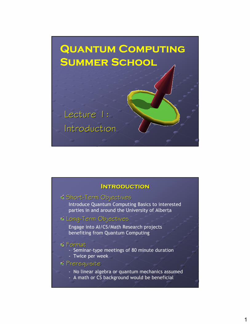
Quantum Computing Summer School
Lecture 1: Lecture 1: IntroductionIntroduction
IntroductionIntroduction
ShortShort--Term ObjectivesTerm Objectives
LongLong--Term ObjectivesTerm Objectives
FormatFormat
PrerequisitePrerequisite
Introduce Quantum Computing Basics to interested parties in and around the University of Alberta
Engage into AI/CS/Math Research projects benefiting from Quantum Computing
- Seminar-type meetings of 80 minute duration- Twice per week
- No linear algebra or quantum mechanics assumed- A math or CS background would be beneficial
2
IntroductionIntroduction
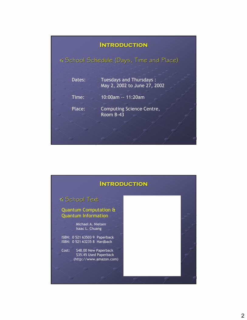
School Schedule (Days, Time and Place)School Schedule (Days, Time and Place)
Dates: Tuesdays and Thursdays : May 2, 2002 to June 27, 2002
Time: 10:00am -- 11:20am
Place: Computing Science Centre, Room B-43
IntroductionIntroduction
School TextSchool Text
Quantum Computation &Quantum Information
Michael A. NielsenIsaac L. Chuang
ISBN: 0 521 63503 9 PaperbackISBN: 0 521 63235 8 Hardback
Cost: $48.00 New Paperback$35.45 Used Paperback
(http://www.amazon.com)
3
IntroductionIntroduction
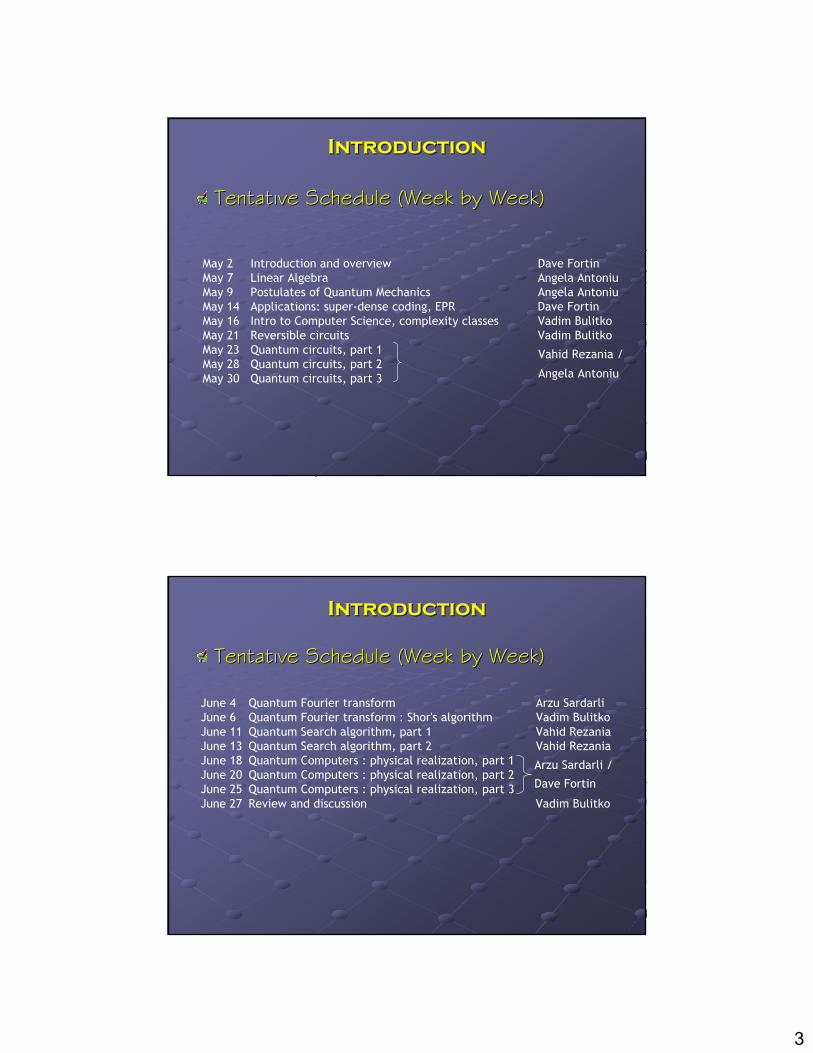
Tentative Schedule (Week by Week)Tentative Schedule (Week by Week)
May 2 Introduction and overview Dave Fortin May 7 Linear Algebra Angela AntoniuMay 9 Postulates of Quantum Mechanics Angela AntoniuMay 14 Applications: super-dense coding, EPR Dave Fortin May 16 Intro to Computer Science, complexity classes Vadim Bulitko May 21 Reversible circuits Vadim Bulitko May 23 Quantum circuits, part 1May 28 Quantum circuits, part 2May 30 Quantum circuits, part 3
Vahid Rezania /
Angela Antoniu
IntroductionIntroduction
Tentative Schedule (Week by Week)Tentative Schedule (Week by Week)
June 4 Quantum Fourier transform Arzu SardarliJune 6 Quantum Fourier transform : Shor's algorithm Vadim Bulitko June 11 Quantum Search algorithm, part 1 Vahid RezaniaJune 13 Quantum Search algorithm, part 2 Vahid RezaniaJune 18 Quantum Computers : physical realization, part 1June 20 Quantum Computers : physical realization, part 2June 25 Quantum Computers : physical realization, part 3 June 27 Review and discussion Vadim Bulitko
Arzu Sardarli /
Dave Fortin
4
IntroductionIntroduction
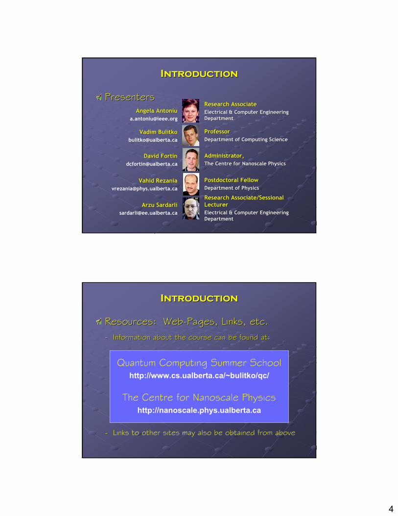
PresentersPresentersAngela Angela AntoniuAntoniu
Vadim BulitkoVadim [email protected]
David FortinDavid [email protected]
VahidVahid [email protected]
ArzuArzu [email protected]
Administrator,Administrator,The The CentreCentre for Nanoscale Physicsfor Nanoscale Physics
ProfessorProfessorDepartment of Computing ScienceDepartment of Computing Science
Research AssociateResearch AssociateElectrical & Computer Engineering Electrical & Computer Engineering DepartmentDepartment
Postdoctoral FellowPostdoctoral FellowDepartment of PhysicsDepartment of Physics
Research Associate/Research Associate/SessionalSessionalLecturer Lecturer Electrical & Computer Engineering Electrical & Computer Engineering DepartmentDepartment
IntroductionIntroduction
Resources: WebResources: Web--Pages, Links, etc.Pages, Links, etc.-- Information about the course can be found at:Information about the course can be found at:
Quantum Computing Summer Schoolhttp://www.cs.ualberta.ca/~bulitko/qc/
The Centre for Nanoscale Physicshttp://nanoscale.phys.ualberta.ca
- Links to other sites may also be obtained from above
5
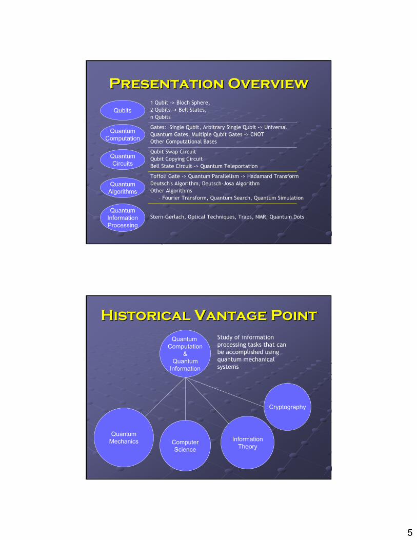
Presentation OverviewPresentation Overview
Qubits
QuantumComputation
QuantumCircuits
QuantumAlgorithms
QuantumInformationProcessing
1 Qubit -> Bloch Sphere, 2 Qubits -> Bell States,n Qubits
Gates: Single Qubit, Arbitrary Single Qubit -> UniversalQuantum Gates, Multiple Qubit Gates -> CNOTOther Computational Bases
Qubit Swap CircuitQubit Copying CircuitBell State Circuit -> Quantum Teleportation
Toffoli Gate -> Quantum Parallelism -> Hadamard TransformDeutsch's Algorithm, Deutsch-Josa AlgorithmOther Algorithms
– Fourier Transform, Quantum Search, Quantum Simulation
Stern-Gerlach, Optical Techniques, Traps, NMR, Quantum Dots
Historical Vantage PointHistorical Vantage PointQuantum
Computation&
QuantumInformation
ComputerScience
InformationTheory
Cryptography
QuantumMechanics
Study of information processing tasks that can be accomplished using quantum mechanical systems
6
What’s a What’s a qubitqubit??
A A qubitqubit has two possible states has two possible states
Unlike bits, a Unlike bits, a quibitquibit can be in a state other thancan be in a state other than
We can form linear combinations of statesWe can form linear combinations of states
A A quibitquibit is a vector in a 2D complex vector is a vector in a 2D complex vector spacespace
0 or 1
0 or 1
0 1ψ α β= +
QubitsQubits
QubitsQubits are computational basis statesare computational basis states-- orthonormalorthonormal basisbasis
-- we cannot examine a bit to determine its we cannot examine a bit to determine its quantum statequantum state
0 for
1 for
ij ij
i ji j
i jδ δ
≠= = =
7
How can a How can a qubitqubit be realized?be realized?
Two polarizations of a photonTwo polarizations of a photon
Alignment of a nuclear spin in a uniform Alignment of a nuclear spin in a uniform magnetic fieldmagnetic field
Two states of an electron orbiting a single Two states of an electron orbiting a single atom (ground or excited state)atom (ground or excited state)
QubitsQubits Cont'dCont'd
We may rewrite as…We may rewrite as…
From a single measurement one obtains From a single measurement one obtains only a single bit of information about the only a single bit of information about the state of the state of the qubitqubitThere is "hidden" quantum information and There is "hidden" quantum information and this info grows exponentiallythis info grows exponentially
0 1ψ α β= +
cos 0 sin 12 2
i ie eα φθ θψ = +
cos 0 sin 12 2
ie φθ θψ = +
We can ignore eiαas it has no observable
effect
8
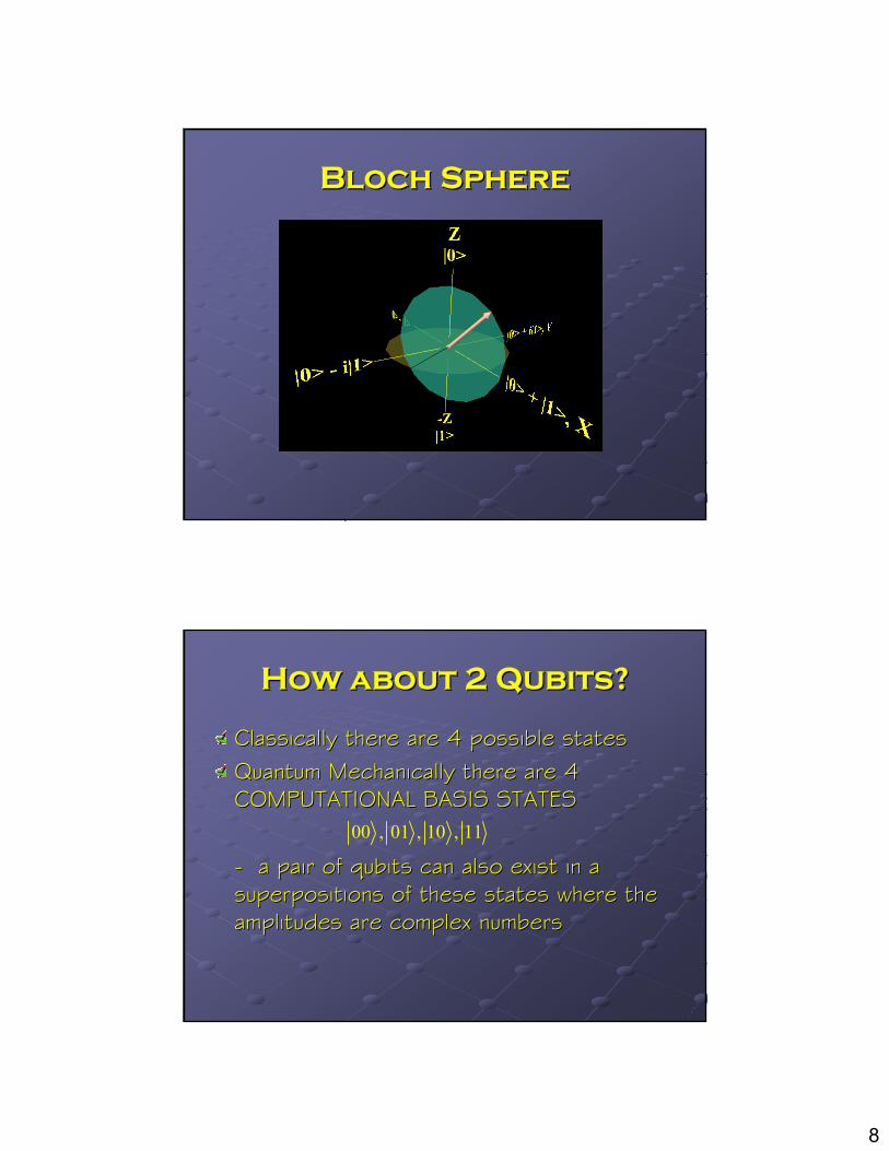
Bloch SphereBloch Sphere
How about 2 How about 2 QubitsQubits??
Classically there are 4 possible statesClassically there are 4 possible statesQuantum Mechanically there are 4 Quantum Mechanically there are 4 COMPUTATIONAL BASIS STATES COMPUTATIONAL BASIS STATES
-- a pair of a pair of qubitsqubits can also exist in a can also exist in a superpositionssuperpositions of these states where the of these states where the amplitudes are complex numbersamplitudes are complex numbers
00 , 01 , 10 , 11
9
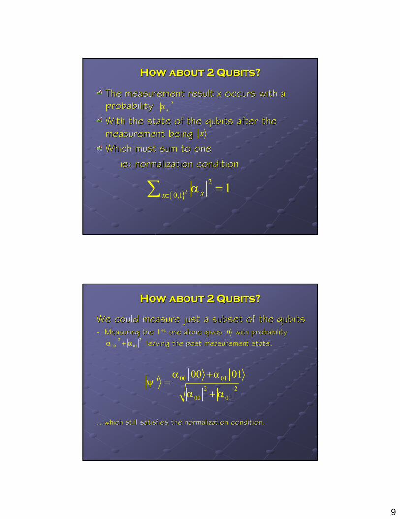
The measurement result x occurs with a The measurement result x occurs with a probability probability With the state of the With the state of the qubitsqubits after the after the measurement being measurement being Which must sum to one Which must sum to one
ieie: normalization condition: normalization condition
How about 2 How about 2 QubitsQubits??
2xα
x
2
2
0,11xx
α∈
=∑
We could measure just a subset of the We could measure just a subset of the qubitsqubits-- Measuring the 1Measuring the 1stst one alone gives with probabilityone alone gives with probability
leaving the post measurement state.leaving the post measurement state.
…which still satisfies the normalization condition.…which still satisfies the normalization condition.
How about 2 How about 2 QubitsQubits??
02 2
00 01α α+
00 01
2 200 01
00 01'
α αψ
α α
+=
+
10
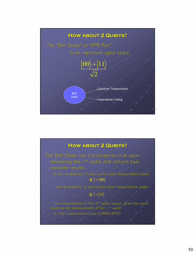
The "Bell State" or "EPR Pair" The "Bell State" or "EPR Pair" is an important is an important qubitqubit state.state.
How about 2 How about 2 QubitsQubits??
00 112+
Quantum Teleportation
Superdense Coding
BellState
The Bell State has the property that upon The Bell State has the property that upon measuring the 1measuring the 1stst qubitqubit one obtains two one obtains two possible results. possible results. -- 0 with probability ½ leaving the post measurement state0 with probability ½ leaving the post measurement state
-- 1 with probability ½ leaving the post measurement state1 with probability ½ leaving the post measurement state
-- The measurement of the 2The measurement of the 2ndnd qubitqubit always gives the same always gives the same result as the measurement of the 1result as the measurement of the 1stst qubitqubit..-- ieie: The measurements are CORRELATED : The measurements are CORRELATED
How about 2 How about 2 QubitsQubits??
' 00φ =
' 11φ =
11
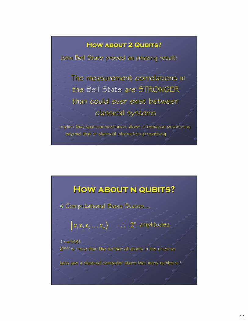
John Bell State proved an amazing result:John Bell State proved an amazing result:
The measurement correlations in The measurement correlations in the the Bell StateBell State are STRONGER are STRONGER than could ever exist between than could ever exist between
classical systemsclassical systems
implies that quantum mechanics allows information processing implies that quantum mechanics allows information processing beyond that of classical information processingbeyond that of classical information processing
How about 2 How about 2 QubitsQubits??
How about n How about n qubitsqubits??
Computational Basis States…Computational Basis States…
amplitudesamplitudes
if n=500 if n=500 22500500 is more than the number of atoms in the universeis more than the number of atoms in the universe
Lets see a classical computer store that many numbers!!!Lets see a classical computer store that many numbers!!!
n1 2 3 2 nx x x x ∴…
12
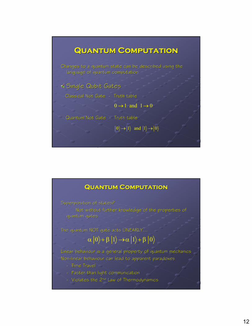
Quantum ComputationQuantum Computation
Changes to a quantum state can be described using the Changes to a quantum state can be described using the language of quantum computationlanguage of quantum computation
Single Single QubitQubit GatesGatesClassical Not GateClassical Not Gate -- Truth tableTruth table
Quantum Not Gate Quantum Not Gate -- Truth tableTruth table
0 1 and 1 0→ →
0 1 and 1 0→ →
Quantum ComputationQuantum Computation
Superposition of states? Superposition of states? Not without further knowledge of the properties of Not without further knowledge of the properties of
quantum gatesquantum gates
The quantum NOT gate acts LINEARLY…The quantum NOT gate acts LINEARLY…
Linear Linear behaviourbehaviour is a general property of quantum mechanicsis a general property of quantum mechanicsNonNon--linear linear behaviourbehaviour can lead to apparent paradoxescan lead to apparent paradoxes
-- Time TravelTime Travel-- Faster than light communicationFaster than light communication-- Violates the 2Violates the 2ndnd Law of ThermodynamicsLaw of Thermodynamics
0 1 1 0α β α β+ → +
13
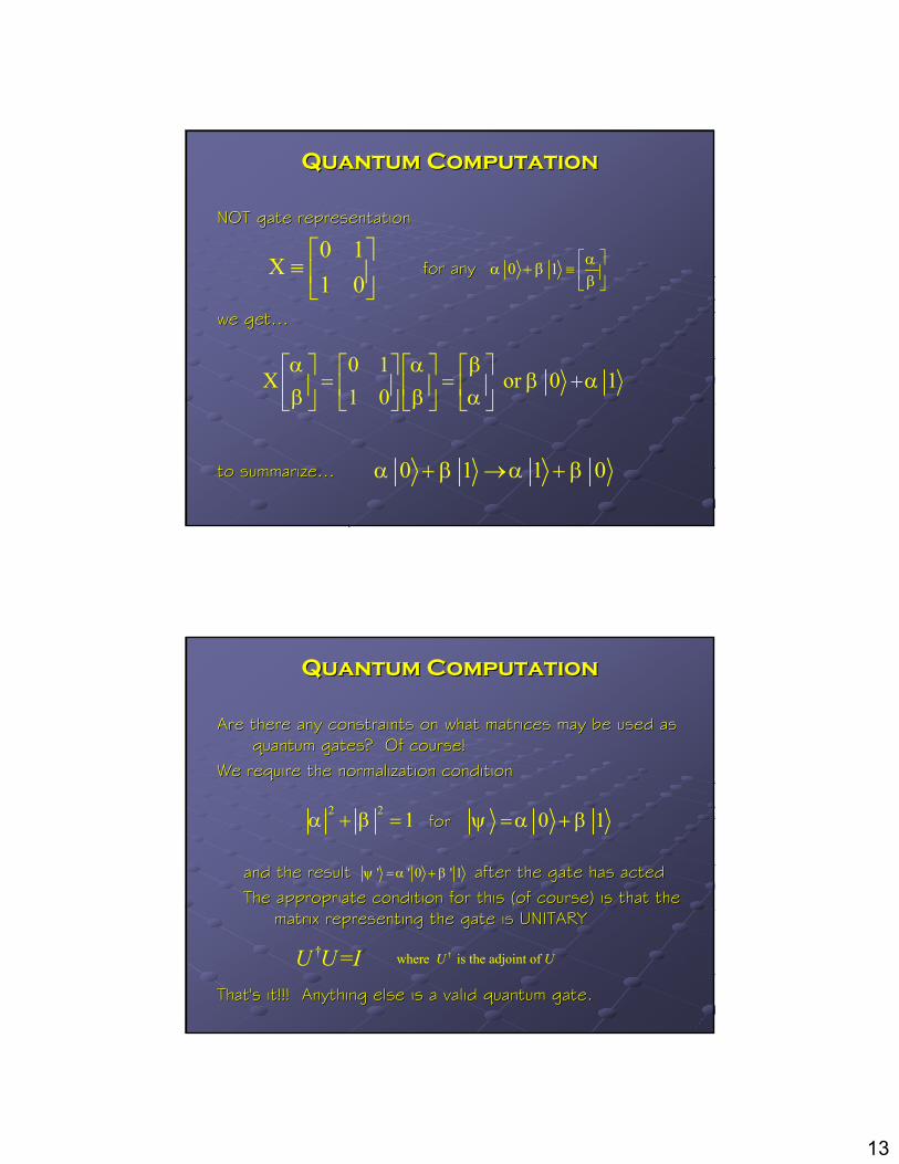
Quantum ComputationQuantum Computation
NOT gate representationNOT gate representation
for anyfor any
we get… we get…
to summarize… to summarize…
0 1X
1 0
≡
0 1 αα β
β
+ ≡
0 1X or 0 1
1 0α α β
β αβ β α
= = +
0 1 1 0α β α β+ → +
Quantum ComputationQuantum Computation
Are there any constraints on what matrices may be used as Are there any constraints on what matrices may be used as quantum gates? Of course!quantum gates? Of course!
We require the normalization conditionWe require the normalization condition
for for
and the result after the gate has actedand the result after the gate has actedThe appropriate condition for this (of course) is that the The appropriate condition for this (of course) is that the
matrix representing the gate is UNITARYmatrix representing the gate is UNITARY
That's it!!! Anything else is a valid quantum gate.That's it!!! Anything else is a valid quantum gate.
2 2 1α β+ = 0 1ψ α β= +
' ' 0 ' 1ψ α β= +
† =U U I †where is the adjoint of U U
14
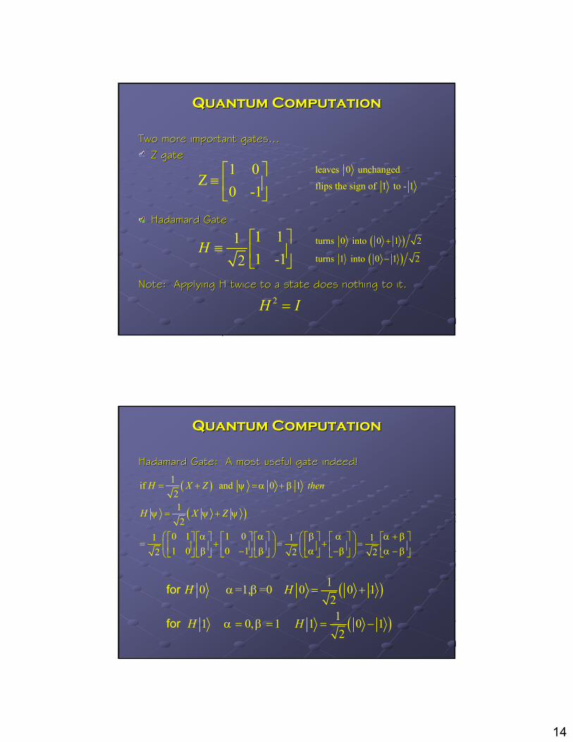
Quantum ComputationQuantum Computation
Two more important gates…Two more important gates…Z gateZ gate
HadamardHadamard GateGate
Note: Applying H twice to a state does nothing to it.Note: Applying H twice to a state does nothing to it.
1 0Z
0 -1
≡
1 111 -12
H ≡
leaves 0 unchanged
flips the sign of 1 to - 1
( )( )
turns 0 into 0 1 2
turns 1 into 0 1 2
+
−
2H I=
Quantum ComputationQuantum Computation
HadamardHadamard Gate: A most useful gate indeed!Gate: A most useful gate indeed!
( )
( )
1 0 =1, =0 0 0 1 21 1 0, 1 1 0 12
H H
H H
α β
α β
= +
= = = −
for
for
( )
( )
1if and 0 1 212
0 1 1 01 1 1 1 0 0 12 2 2
H X Z then
H X Z
ψ α β
ψ ψ ψ
α α β α α ββ β α β α β
= + = +
= +
+ = + = + = − − −
15
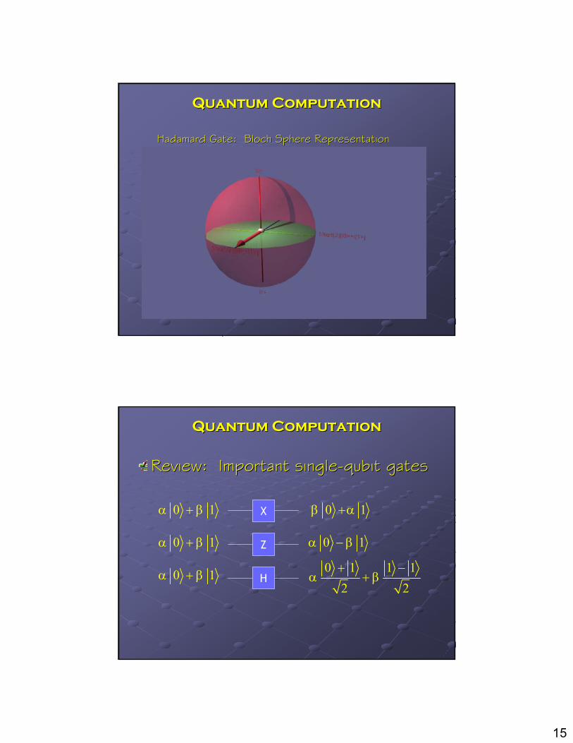
Quantum ComputationQuantum Computation
HadamardHadamard Gate: Bloch Sphere RepresentationGate: Bloch Sphere Representation
Quantum ComputationQuantum Computation
Review: Important singleReview: Important single--qubitqubit gatesgates
0 1α β+
0 1α β+
0 1α β+
X
Z
H
0 1β α+
0 1α β−
0 1 1 12 2
α β+ −
+
16
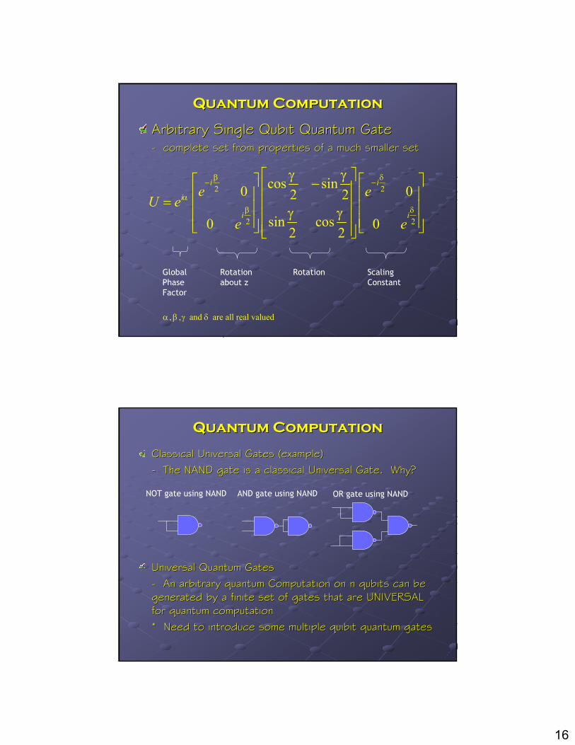
Quantum ComputationQuantum Computation
Arbitrary Single Arbitrary Single QubitQubit Quantum GateQuantum Gate-- complete set from properties of a much smaller setcomplete set from properties of a much smaller set
2 2
2 2
cos sin0 02 2
sin cos0 02 2
i i
i
i i
e eU e
e e
β δ
α
β δ
γ γ
γ γ
− − − =
Global Phase Factor
Rotation about z
Rotation Scaling Constant
, , and are all real valuedα β γ δ
Quantum ComputationQuantum Computation
Classical Universal Gates (example)Classical Universal Gates (example)-- The NAND gate is a classical Universal Gate. Why?The NAND gate is a classical Universal Gate. Why?
Universal Quantum GatesUniversal Quantum Gates-- An arbitrary quantum Computation on n An arbitrary quantum Computation on n qubitsqubits can be can be generated by a finite set of gates that are UNIVERSAL generated by a finite set of gates that are UNIVERSAL for quantum computationfor quantum computation* Need to introduce some multiple * Need to introduce some multiple quibitquibit quantum gatesquantum gates
NOT gate using NAND AND gate using NAND OR gate using NAND
17
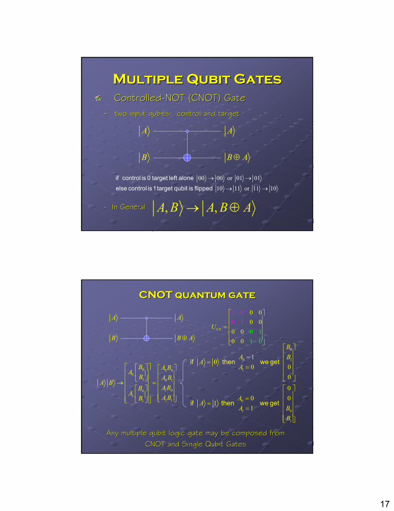
Multiple Multiple QubitQubit GatesGatesControlledControlled--NOT (CNOT) GateNOT (CNOT) Gate
-- two input two input qubitsqubits: control and target: control and target
-- In GeneralIn General
A
B
A
B A⊕
00 00 or 01 01
10 11 or 11 10
→ →
→ →
if control is 0 target left alone else control is 1 target qubit is flipped
, ,A B A B A→ ⊕
CNOT quantum gateCNOT quantum gate
A
B
A
B A⊕
0 00 0
0 00
0 11 0
0
0
10 1
CNU
=
0
0 1
0 10 00
1 0 1
1 001
1 1 01
1 0
1
1 0
0 00
0
0 0 1
1
BA B
AB AA BAB A B
A BABB
AAB AB
AA B
B
= = = → = = = =
if then we get
if then we get
Any multiple Any multiple qubitqubit logic gate may be composed from logic gate may be composed from CNOT and Single CNOT and Single QubitQubit GatesGates
18
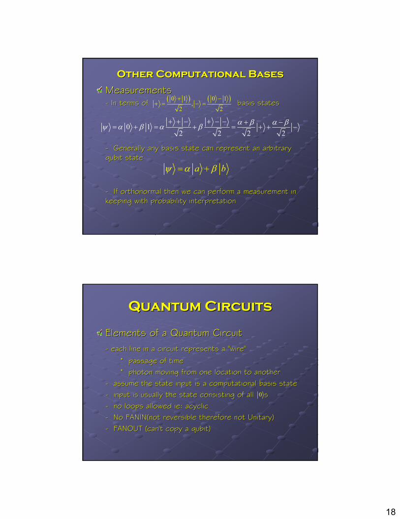
Other Computational BasesOther Computational Bases
MeasurementsMeasurements-- In terms of basis statesIn terms of basis states
-- Generally any basis state can represent an arbitrary Generally any basis state can represent an arbitrary qubitqubit statestate
-- If If orthonormalorthonormal then we can perform a measurement in then we can perform a measurement in keeping with probability interpretationkeeping with probability interpretation
0 12 2 2 2
α β α βψ α β α β+ + − + − − + −
= + = + = + + −
( ) ( )0 1 0 1,
2 2
+ −+ = − =
a bψ α β= +
Quantum CircuitsQuantum Circuits
Elements of a Quantum CircuitElements of a Quantum Circuit-- each line in a circuit represents a "wire" each line in a circuit represents a "wire"
* passage of time * passage of time * photon moving from one location to another* photon moving from one location to another
-- assume the state input is a computational basis stateassume the state input is a computational basis state-- input is usually the state consisting of all sinput is usually the state consisting of all s-- no loops allowed no loops allowed ieie: : acyclicacyclic-- No No FANIN(notFANIN(not reversible therefore not Unitary) reversible therefore not Unitary) -- FANOUT (can't copy a FANOUT (can't copy a qubitqubit))
0
19
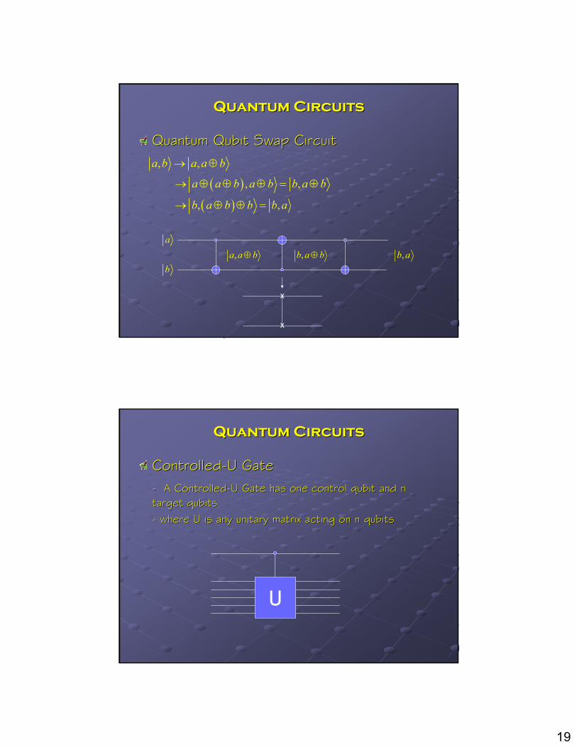
Quantum CircuitsQuantum Circuits
Quantum Quantum QubitQubit Swap CircuitSwap Circuit
( )( )
, ,
, ,
, ,
a b a a b
a a b a b b a b
b a b b b a
→ ⊕
→ ⊕ ⊕ ⊕ = ⊕
→ ⊕ ⊕ =
a
b,b a,b a b⊕,a a b⊕
x
x
Quantum CircuitsQuantum Circuits
ControlledControlled--U GateU Gate-- A ControlledA Controlled--U Gate has one control U Gate has one control qubitqubit and n and n target target qubitsqubits-- where U is any unitary matrix acting on n where U is any unitary matrix acting on n qubitsqubits
U
20
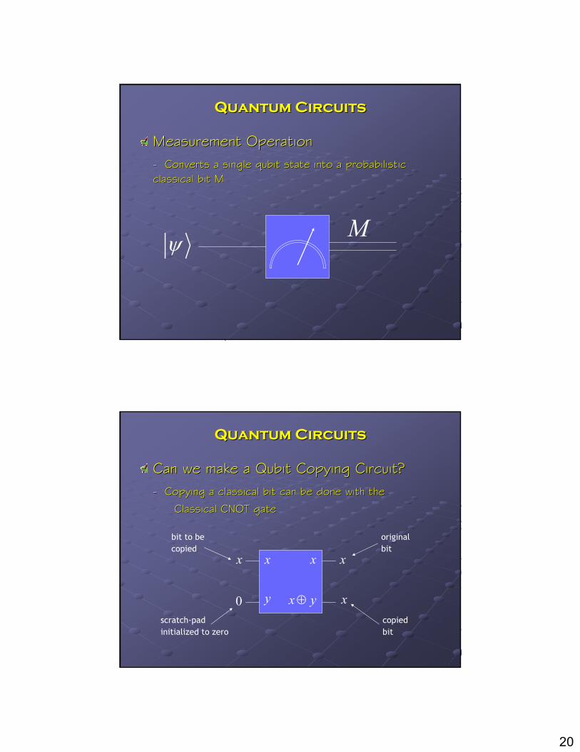
Quantum CircuitsQuantum Circuits
Measurement OperationMeasurement Operation-- Converts a single Converts a single qubitqubit state into a probabilistic state into a probabilistic classical bit Mclassical bit M
ψM
Quantum CircuitsQuantum Circuits
Can we make a Can we make a QubitQubit Copying Circuit?Copying Circuit?-- Copying a classical bit can be done with the Copying a classical bit can be done with the
Classical CNOT gateClassical CNOT gate
x
0
x
x
x x
y x y⊕scratch-padinitialized to zero
bit to becopied
originalbit
copiedbit
21
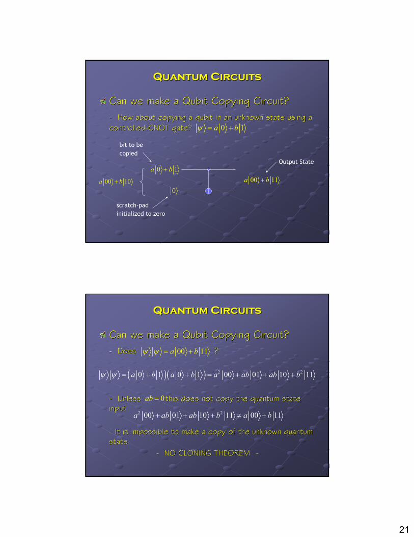
Quantum CircuitsQuantum Circuits
Can we make a Can we make a QubitQubit Copying Circuit?Copying Circuit?-- How about copying a How about copying a qubitqubit in an unknown state using a in an unknown state using a controlledcontrolled--CNOT gate?CNOT gate?
scratch-padinitialized to zero
bit to becopied
Output State
0 1a bψ = +
0 1a b+
000 11a b+00 10a b+
Quantum CircuitsQuantum Circuits
Can we make a Can we make a QubitQubit Copying Circuit?Copying Circuit?-- Does ?Does ?
-- Unless this does not copy the quantum state Unless this does not copy the quantum state input input
-- It is impossible to make a copy of the unknown quantum It is impossible to make a copy of the unknown quantum statestate
-- NO CLONING THEOREM NO CLONING THEOREM --
00 11a bψ ψ = +
( )( ) 2 20 1 0 1 00 01 10 11a b a b a ab ab bψ ψ = + + = + + +
0ab =
2 200 01 10 11 00 11a ab ab b a b+ + + ≠ +
22
Quantum CircuitsQuantum Circuits
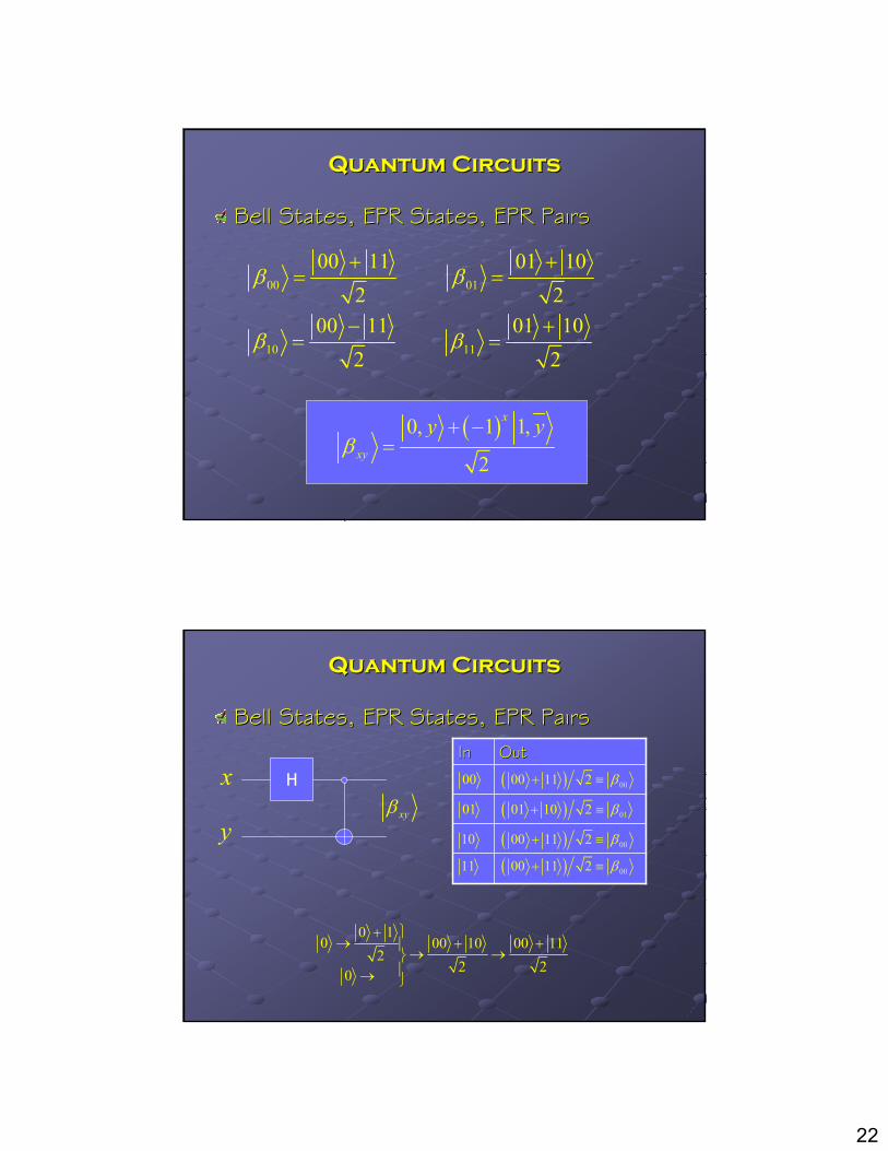
Bell States, EPR States, EPR PairsBell States, EPR States, EPR Pairs
00 01
10 11
00 11 01 10
2 200 11 01 10
2 2
β β
β β
+ += =
− += =
( )0, 1 1,
2
x
xy
y yβ
+ −=
Quantum CircuitsQuantum Circuits
Bell States, EPR States, EPR PairsBell States, EPR States, EPR Pairs
x H
xyβy
0 10 00 10 00 11
22 20
+ → + +→ →
→
OutOutInIn00
01
10
11
( ) 0000 11 2 β+ ≡
( ) 0101 10 2 β+ ≡
( ) 0000 11 2 β+ ≡
( ) 0000 11 2 β+ ≡
23
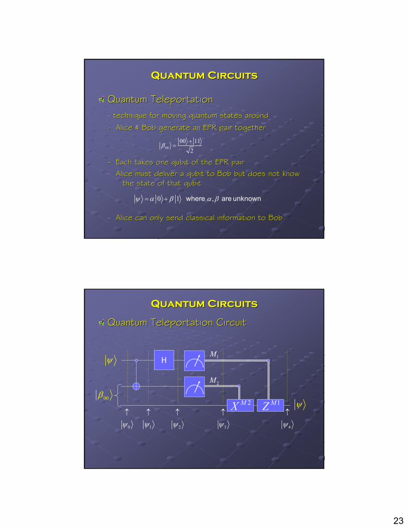
Quantum CircuitsQuantum Circuits
Quantum TeleportationQuantum Teleportation-- technique for moving quantum states aroundtechnique for moving quantum states around
-- Alice & Bob generate an EPR pair togetherAlice & Bob generate an EPR pair together
-- Each takes one Each takes one qubitqubit of the EPR pairof the EPR pair-- Alice must deliver a Alice must deliver a qubitqubit to Bob but does not know to Bob but does not know
the state of that the state of that qubitqubit
-- Alice can only send classical information to Bob Alice can only send classical information to Bob
00
00 112
β+
=
0 1 , ψ α β α β= + where are unknown
Quantum CircuitsQuantum Circuits
Quantum Teleportation CircuitQuantum Teleportation Circuit
H
ψ
1M
2M
2MX 1MZ
ψ
00β
0ψ↑
1ψ↑
2ψ↑
3ψ↑
4ψ↑
24
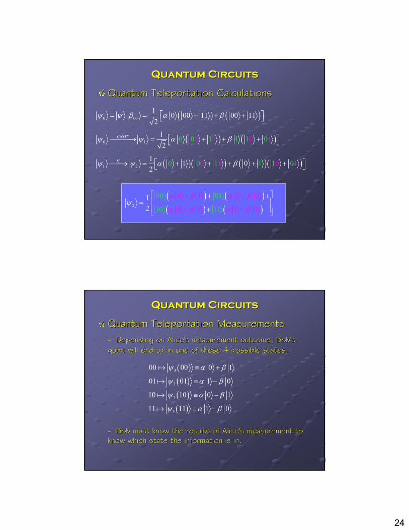
Quantum CircuitsQuantum Circuits
Quantum Teleportation CalculationsQuantum Teleportation Calculations
( ) ( )0 001 0 00 11 00 112
ψ ψ β α β = = + + +
( ) ( )0 1 0 00 1 01 12
1 011CNOTψ ψ α β → = + + +
( )( ) ( )( )1 21 1 00 0 1 1 102
1 0 01Hψ ψ α β → = + + + + +
( ) ( )( ) ( )2
00 01
101 0 1 1 0
02 1 011 1
α β α β
αψ
β α β
+ −
−
+ + =
+ −
Quantum CircuitsQuantum Circuits
Quantum Teleportation MeasurementsQuantum Teleportation Measurements-- Depending on Alice's measurement outcome, Bob's Depending on Alice's measurement outcome, Bob's qubitqubit will end up in one of these 4 possible states.will end up in one of these 4 possible states.
-- Bob must know the results of Alice's measurement to Bob must know the results of Alice's measurement to know which state the information is in.know which state the information is in.
( )( )( )( )
3
3
3
3
00 00 0 1
01 01 1 0
10 10 0 1
11 11 1 0
ψ α β
ψ α β
ψ α β
ψ α β
≡ +
≡ −
≡ −
≡ −
25
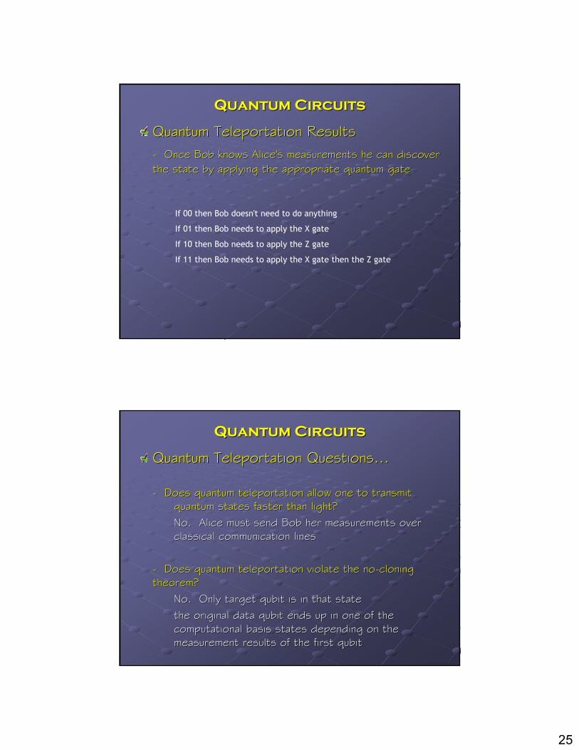
Quantum CircuitsQuantum Circuits
Quantum Teleportation ResultsQuantum Teleportation Results-- Once Bob knows Alice's measurements he can discover Once Bob knows Alice's measurements he can discover the state by applying the appropriate quantum gatethe state by applying the appropriate quantum gate
If 00 then Bob doesn't need to do anything
If 01 then Bob needs to apply the X gate
If 10 then Bob needs to apply the Z gate
If 11 then Bob needs to apply the X gate then the Z gate
Quantum CircuitsQuantum Circuits
Quantum Teleportation Questions…Quantum Teleportation Questions…
-- Does quantum teleportation allow one to transmit Does quantum teleportation allow one to transmit quantum states faster than light?quantum states faster than light?No. Alice must send Bob her measurements over No. Alice must send Bob her measurements over classical communication linesclassical communication lines
-- Does quantum teleportation violate the noDoes quantum teleportation violate the no--cloning cloning theorem?theorem?
No. Only target No. Only target qubitqubit is in that state is in that state the original data the original data qubitqubit ends up in one of the ends up in one of the computational basis states depending on the computational basis states depending on the measurement results of the first measurement results of the first qubitqubit
26
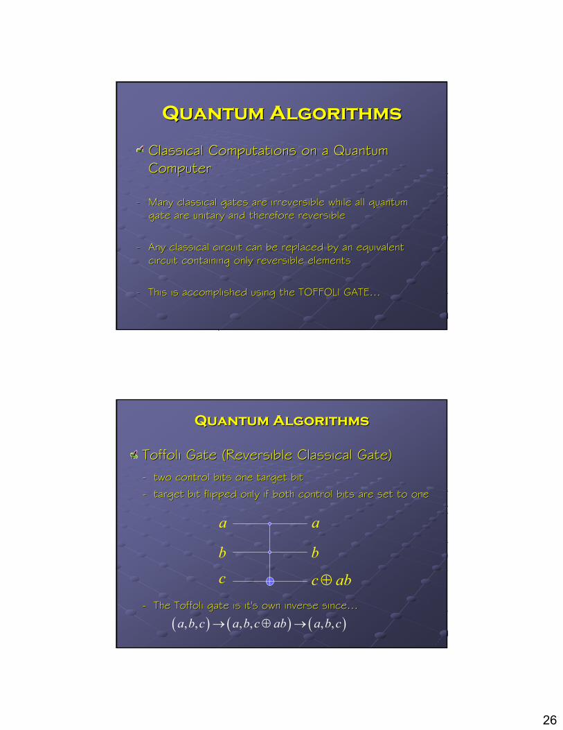
Quantum AlgorithmsQuantum Algorithms
Classical Computations on a Quantum Classical Computations on a Quantum ComputerComputer
-- Many classical gates are irreversible while all quantum Many classical gates are irreversible while all quantum gate are unitary and therefore reversiblegate are unitary and therefore reversible
-- Any classical circuit can be replaced by an equivalent Any classical circuit can be replaced by an equivalent circuit containing only reversible elementscircuit containing only reversible elements
-- This is accomplished using the TOFFOLI GATE…This is accomplished using the TOFFOLI GATE…
Quantum AlgorithmsQuantum Algorithms
ToffoliToffoli Gate (Reversible Classical Gate)Gate (Reversible Classical Gate)-- two control bits one target bittwo control bits one target bit
-- target bit flipped only if both control bits are set to onetarget bit flipped only if both control bits are set to one
-- The The ToffoliToffoli gate is it's own inverse since…gate is it's own inverse since…
a
bc
a
b
c ab⊕
( ) ( ) ( ), , , , , ,a b c a b c ab a b c→ ⊕ →
27
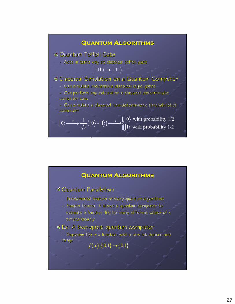
Quantum AlgorithmsQuantum Algorithms
Quantum Quantum ToffoliToffoli Gate Gate -- Acts in same way as classical Acts in same way as classical toffolitoffoli gategate
Classical Simulation on a Quantum ComputerClassical Simulation on a Quantum Computer-- Can simulate irreversible classical logic gatesCan simulate irreversible classical logic gates-- Can perform any calculation a classical deterministic Can perform any calculation a classical deterministic computer can.computer can.-- Can simulate a classical nonCan simulate a classical non--deterministic (probabilistic) deterministic (probabilistic) computercomputer
110 111→
( ) 0 with probability 1/210 0 11 with probability 1/22
H M → + →
Quantum AlgorithmsQuantum Algorithms
Quantum ParallelismQuantum Parallelism-- Fundamental feature of many quantum algorithmsFundamental feature of many quantum algorithms
-- Simple Terms: it allows a quantum computer to Simple Terms: it allows a quantum computer to evaluate a function evaluate a function f(xf(x) for many different values of x ) for many different values of x simultaneouslysimultaneously
Ex: A twoEx: A two--qubitqubit quantum computerquantum computer-- Suppose Suppose f(xf(x) is a function with a one) is a function with a one--bit domain and bit domain and rangerange
( ) : 0,1 0,1f x →
28
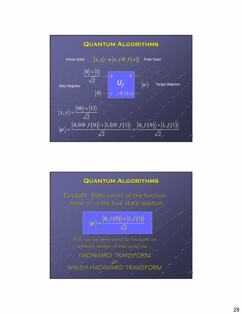
Quantum AlgorithmsQuantum Algorithms
( ), ,x y x y f x→ ⊕
Data Register Target Register
Initial State Final State
00 11,
2x y
+=
0 12+
0
x x
y ( )y f x⊕
ψ
( ) ( ) ( ) ( )0,0 0 1,0 1 0, 0 1, 1
2 2
f f f fψ
⊕ + ⊕ += =
Uf
Eureka!!!! Both values of the function Eureka!!!! Both values of the function show up in the final state solution.show up in the final state solution.
This can be generalized to functions on This can be generalized to functions on arbitrary number of bits using the… arbitrary number of bits using the…
HADAMARD TRANSFORM HADAMARD TRANSFORM or or
WALSHWALSH--HADAMARD TRANSFORM HADAMARD TRANSFORM
Quantum AlgorithmsQuantum Algorithms
( ) ( )0, 0 1, 1
2
f fψ
+=
29
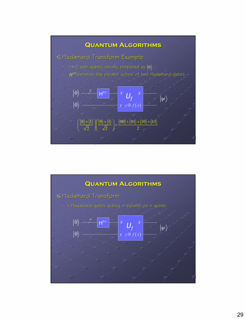
Quantum AlgorithmsQuantum Algorithms
HadamardHadamard Transform Example Transform Example -- n=2 with n=2 with qubitsqubits initially prepared asinitially prepared as
-- denotes the parallel action of two denotes the parallel action of two HadamardHadamard gates gates 0
2H ⊗
0 1 0 1 00 01 10 1122 2
+ + + + +=
0
0 y ( )y f x⊕ψ
x2 2⊗H xUf
Quantum AlgorithmsQuantum Algorithms
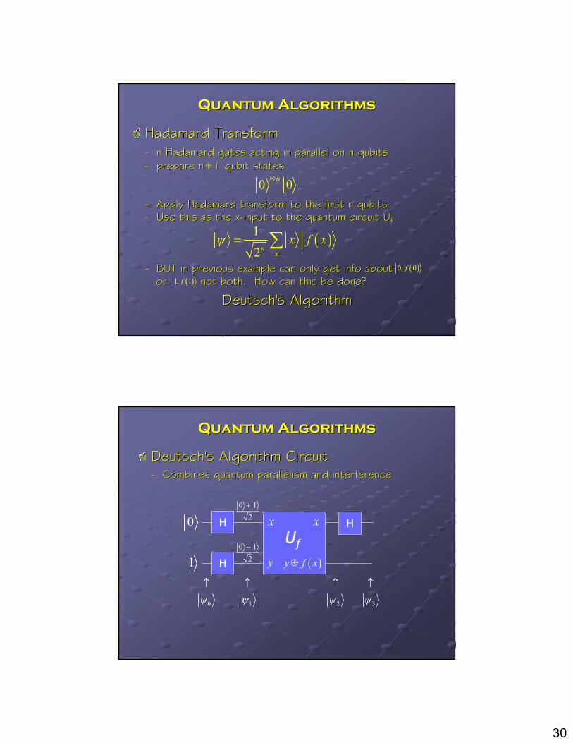
HadamardHadamard Transform Transform -- n n HadamardHadamard gates acting in parallel on n gates acting in parallel on n qubitsqubits
0
0 y ( )y f x⊕ψ
xnn⊗H xUf
30
Quantum AlgorithmsQuantum Algorithms
HadamardHadamard Transform Transform -- n n HadamardHadamard gates acting in parallel on n gates acting in parallel on n qubitsqubits-- prepare n+1 prepare n+1 qubitqubit statesstates
-- Apply Apply HadamardHadamard transform to the first n transform to the first n qubitsqubits-- Use this as the xUse this as the x--input to the quantum circuit Uinput to the quantum circuit Uff
-- BUT in previous example can only get info aboutBUT in previous example can only get info aboutor not both. How can this be done? or not both. How can this be done?
Deutsch's AlgorithmDeutsch's Algorithm
0 0n⊗
( )12n x
x f xψ = ∑( )0, 0f
( )1, 1f
Quantum AlgorithmsQuantum Algorithms
Deutsch's Algorithm CircuitDeutsch's Algorithm Circuit-- Combines quantum parallelism and interferenceCombines quantum parallelism and interference
0 12+
x x
y ( )y f x⊕
0 H
1 H
0 12−
0ψ↑
1ψ↑
2ψ↑
3ψ↑
HUf
31
Quantum AlgorithmsQuantum Algorithms
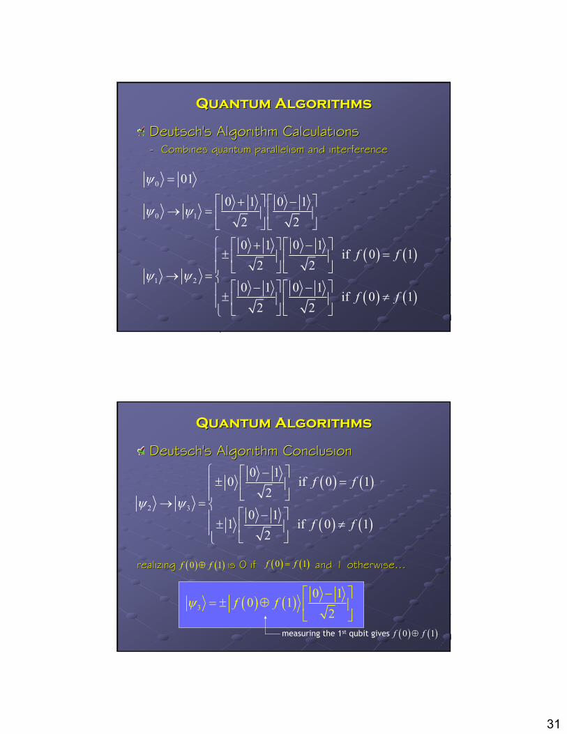
Deutsch's Algorithm CalculationsDeutsch's Algorithm Calculations-- Combines quantum parallelism and interferenceCombines quantum parallelism and interference
0 01ψ =
0 1
0 1 0 12 2
ψ ψ + −
→ =
( ) ( )
( ) ( )1 2
0 1 0 1 if 0 1
2 2
0 1 0 1 if 0 1
2 2
f f
f fψ ψ
+ − ± = → =
− − ± ≠
Quantum AlgorithmsQuantum Algorithms
Deutsch's Algorithm ConclusionDeutsch's Algorithm Conclusion
realizing is 0 if and 1 otherwise… realizing is 0 if and 1 otherwise…
( ) ( )
( ) ( )2 3
0 10 if 0 1
2
0 11 if 0 1
2
f f
f fψ ψ
− ± = → =
− ± ≠
( ) ( )3
0 10 1
2f fψ
− = ± ⊕
( ) ( )0 1f f⊕ ( ) ( )0 1f f=
measuring the 1st qubit gives ( ) ( )0 1f f⊕
32
Quantum AlgorithmsQuantum Algorithms
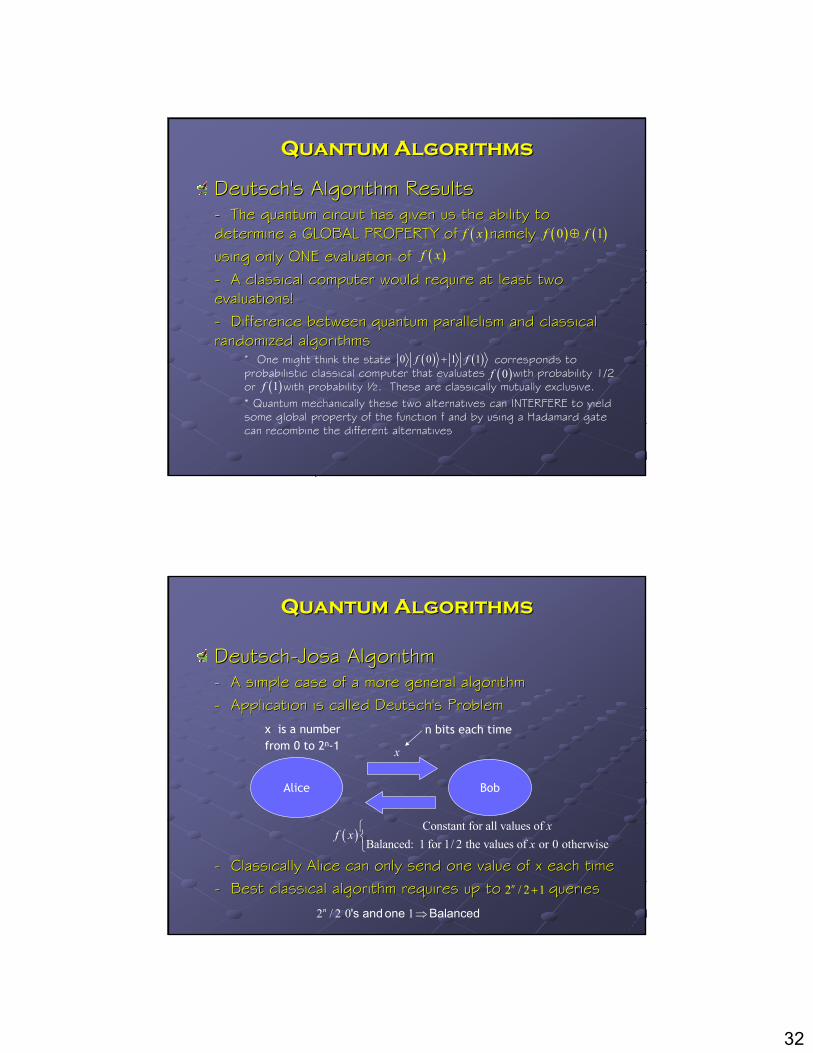
Deutsch's Algorithm ResultsDeutsch's Algorithm Results-- The quantum circuit has given us the ability to The quantum circuit has given us the ability to determine a GLOBAL PROPERTY of namelydetermine a GLOBAL PROPERTY of namelyusing only ONE evaluation ofusing only ONE evaluation of-- A classical computer would require at least two A classical computer would require at least two evaluations! evaluations! -- Difference between quantum parallelism and classical Difference between quantum parallelism and classical randomized algorithmsrandomized algorithms
* * One might think the state corresponds to probabilistic classical computer that evaluates with probability 1/2 or with probability ½. These are classically mutually exclusive.* Quantum mechanically these two alternatives can INTERFERE to yield some global property of the function f and by using a Hadamard gate can recombine the different alternatives
( ) ( )0 1f f⊕( )f x
( )f x
( ) ( )0 0 1 1f f+( )0f
( )1f
DeutschDeutsch--JosaJosa AlgorithmAlgorithm-- A simple case of a more general algorithmA simple case of a more general algorithm-- Application is called Deutsch's ProblemApplication is called Deutsch's Problem
-- Classically Alice can only send one value of x each timeClassically Alice can only send one value of x each time-- Best classical algorithm requires up to queriesBest classical algorithm requires up to queries
Quantum AlgorithmsQuantum Algorithms
Alice Bob
x is a number from 0 to 2n-1
( )Constant for all values of
Balanced: 1 for 1/ 2 the values of or 0 otherwisex
f xx
x
2 / 2 0 1n ⇒'s and one Balanced
2 / 2 1n +
n bits each time
33
DeutschDeutsch--JosaJosa AlgorithmAlgorithm-- If Bob and Alice were able to exchange If Bob and Alice were able to exchange qubitsqubits instead instead of classical bits and if Bob calculated of classical bits and if Bob calculated f(xf(x)) using a unitary using a unitary transform transform UUff then Alice could determine the function in then Alice could determine the function in one query.one query.-- Alice has an n Alice has an n qubitqubit register and a single register and a single qubitqubit register register which she gives to Bobwhich she gives to Bob-- Prepares query and answer register in a superposition Prepares query and answer register in a superposition statestate-- Bob evaluates Bob evaluates f(xf(x) and puts result into answer register) and puts result into answer register-- Alice interferes the states in the superposition using a Alice interferes the states in the superposition using a hadamardhadamard transform on the query registertransform on the query register
Quantum AlgorithmsQuantum Algorithms
1ψ
2ψ
3ψ
0ψ
Quantum AlgorithmsQuantum Algorithms
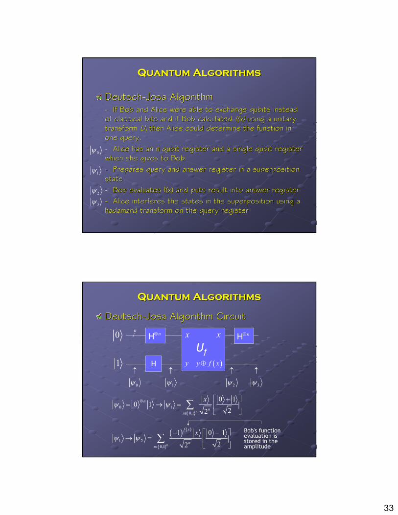
DeutschDeutsch--JosaJosa Algorithm CircuitAlgorithm Circuit
x x
y ( )y f x⊕
0
1 H
0ψ↑
1ψ↑
2ψ↑
3ψ↑
nn⊗H
Uf
n⊗H
0 1
0,1
0 10 1
22n
n
nx
xψ ψ⊗
∈
+ = → =
∑
( ) ( )
1 2
0,1
1 0 122n
f x
nx
xψ ψ
∈
− − → =
∑
Bob's function evaluation is stored in the amplitude
34
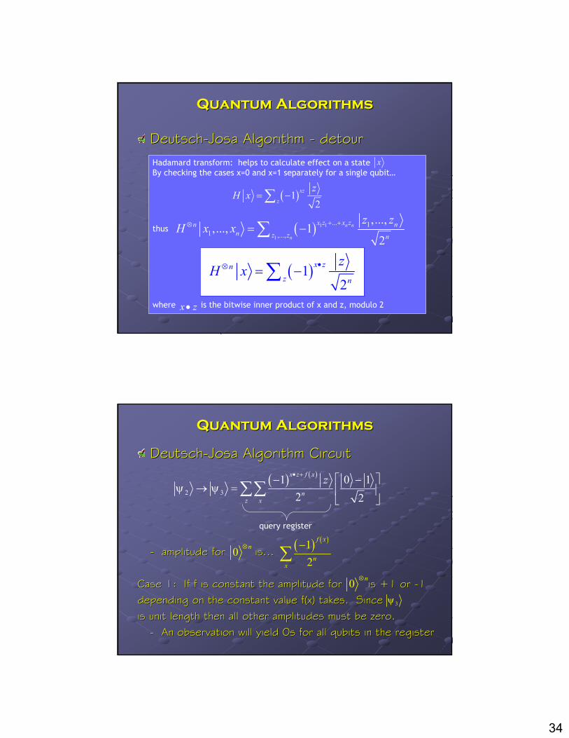
Hadamard transform: helps to calculate effect on a state By checking the cases x=0 and x=1 separately for a single qubit…
thus
where is the bitwise inner product of x and z, modulo 2
Quantum AlgorithmsQuantum Algorithms
DeutschDeutsch--JosaJosa Algorithm Algorithm -- detourdetourx
( )12
xz
z
zH x = −∑
( ) 1 1
1
... 11 ,...,
,...,,..., 1
2n n
n
x z x z nnn z z n
z zH x x + +⊗ = −∑
( )12
x znz n
zH x •⊗ = −∑
x z•
Quantum AlgorithmsQuantum Algorithms
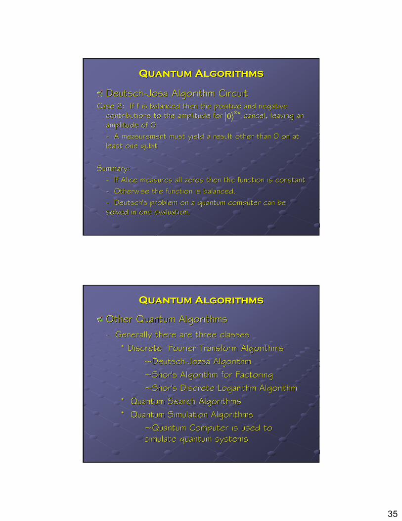
DeutschDeutsch--JosaJosa Algorithm CircuitAlgorithm Circuit
-- amplitude for is…amplitude for is…
Case 1: If f is constant the amplitude for is +1 or Case 1: If f is constant the amplitude for is +1 or --11depending on the constant value depending on the constant value f(xf(x) takes. Since) takes. Sinceis unit length then all other amplitudes must be zero.is unit length then all other amplitudes must be zero.
-- An observation will yield 0s for all An observation will yield 0s for all qubitsqubits in the register in the register
( ) ( )
2 3
1 0 12 2
x z f x
nz x
zψ ψ
• +− − → =
∑∑
query register
0 n⊗ ( ) ( )12
f x
nx
−∑
0 n⊗
3ψ
35
Quantum AlgorithmsQuantum Algorithms
DeutschDeutsch--JosaJosa Algorithm CircuitAlgorithm CircuitCase 2: If f is balanced then the positive and negative Case 2: If f is balanced then the positive and negative
contributions to the amplitude for cancel, leaving an contributions to the amplitude for cancel, leaving an amplitude of 0amplitude of 0-- A measurement must yield a result other than 0 on at A measurement must yield a result other than 0 on at least one least one qubitqubit
Summary: Summary: -- If Alice measures all zeros then the function is constantIf Alice measures all zeros then the function is constant-- Otherwise the function is balanced.Otherwise the function is balanced.-- Deutsch's problem on a quantum computer can be Deutsch's problem on a quantum computer can be solved in one evaluation. solved in one evaluation.
0 n⊗
Quantum AlgorithmsQuantum Algorithms
Other Quantum AlgorithmsOther Quantum Algorithms-- Generally there are three classesGenerally there are three classes
* Discrete * Discrete Fourier Transform AlgorithmsFourier Transform Algorithms~Deutsch~Deutsch--JozsaJozsa AlgorithmAlgorithm~~Shor'sShor's Algorithm for FactoringAlgorithm for Factoring~~Shor'sShor's Discrete Logarithm AlgorithmDiscrete Logarithm Algorithm
* Quantum Search Algorithms* Quantum Search Algorithms* Quantum Simulation Algorithms* Quantum Simulation Algorithms
~Quantum Computer is used to ~Quantum Computer is used to simulate quantum systemssimulate quantum systems
36
Experimental Quantum Experimental Quantum Information ProcessingInformation Processing
The SternThe Stern--GerlachGerlach ExperimentExperimentOptical TechniquesOptical TechniquesNuclear Magnetic ResonanceNuclear Magnetic ResonanceQuantum DotsQuantum DotsTraps: Ion Traps & Neutral Atom TrapsTraps: Ion Traps & Neutral Atom Traps
Thanks!Thanks!
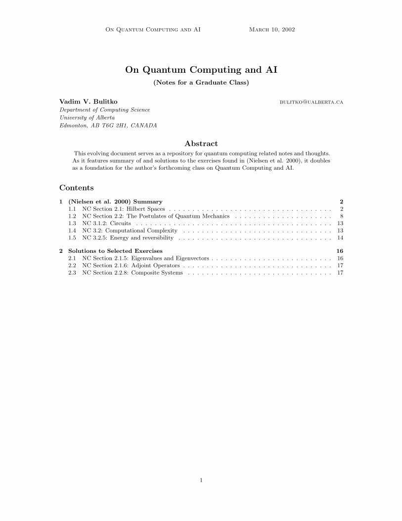
On Quantum Computing and AI March 10, 2002
On Quantum Computing and AI(Notes for a Graduate Class)
Vadim V. Bulitko [email protected]
Department of Computing Science
University of Alberta
Edmonton, AB T6G 2H1, CANADA
AbstractThis evolving document serves as a repository for quantum computing related notes and thoughts.As it features summary of and solutions to the exercises found in (Nielsen et al. 2000), it doublesas a foundation for the author’s forthcoming class on Quantum Computing and AI.
Contents
1 (Nielsen et al. 2000) Summary 21.1 NC Section 2.1: Hilbert Spaces . . . . . . . . . . . . . . . . . . . . . . . . . . . . . . . . . . . 21.2 NC Section 2.2: The Postulates of Quantum Mechanics . . . . . . . . . . . . . . . . . . . . . 81.3 NC 3.1.2: Circuits . . . . . . . . . . . . . . . . . . . . . . . . . . . . . . . . . . . . . . . . . . 131.4 NC 3.2: Computational Complexity . . . . . . . . . . . . . . . . . . . . . . . . . . . . . . . . 131.5 NC 3.2.5: Energy and reversibility . . . . . . . . . . . . . . . . . . . . . . . . . . . . . . . . . 14
2 Solutions to Selected Exercises 162.1 NC Section 2.1.5: Eigenvalues and Eigenvectors . . . . . . . . . . . . . . . . . . . . . . . . . . 162.2 NC Section 2.1.6: Adjoint Operators . . . . . . . . . . . . . . . . . . . . . . . . . . . . . . . . 172.3 NC Section 2.2.8: Composite Systems . . . . . . . . . . . . . . . . . . . . . . . . . . . . . . . 17
1
March 10, 2002 Vadim Bulitko
1. (Nielsen et al. 2000) Summary
The purpose of this section is to provide a highly compressed collection of facts presented in(Nielsen et al. 2000). This is helpful when refreshing material in the past sections.
1.1 NC Section 2.1: Hilbert Spaces
Complex numbers are specified by the real and imaginary parts: a + ib where a, b ∈ R andi2 = −1.
Polar representation: ueiθ = u(cos θ + i sin θ) where θ, u ∈ R and u is called the modulus of thecomplex number.
Complex conjugate: (a+ ib)∗ = a− ib.
Vectors are represented by columns: |v〉 =[v1v2
].
Dual vectors are represented by rows: |v〉† = 〈v| = [v∗1 , v∗2 ].
Matrix multiplication: each element of the new matrix is a sum of products of the first factor’s
row and the second factor’s column rotated to be superimposed on top of the row:[a1 a2
a3 a4
]×[
xy
]=
[a1x+ a2ya3x+ a4y
].
Linear dependence: non-zero vectors |v1〉 , . . . , |vn〉 are linearly dependent iff at least one of themis expressible through the others: |vj〉 =
∑i ai |vi〉 where am ∈ C.
The Pauli matrices: are given as:
• σ0 = I =[
1 00 1
];
• σ1 = σx = X =[
0 11 0
]• σ2 = σy = Y =
[0 −ii 0
]• σ3 = σz = Z =
[1 00 −1
].
Properties:
1. unitary: (σk)†σk = I for all k;
2. Hermitian: (σk)† = σk for all k;
3. eigen-decomposition:
(a) σ0 = I =[
1 00 1
]has the following eigenvectors: |0〉 with the eigenvalue of 1 and
|1〉 with the eigenvalue of 1. Thus:
I =[
1 00 1
](1.1.1)
= 1 · |0〉 〈0|+ 1 · |1〉 〈1| (1.1.2)= |0〉 〈0|+ |1〉 〈1|. (1.1.3)
2
On Quantum Computing and AI March 10, 2002
(b) σ1 = σx = X =[
0 11 0
]has the following eigenvectors: |0〉+|1〉√
2with the eigenvalue
of 1 and |0〉−|1〉√2
with the eigenvalue of −1. Thus:
X =[
0 11 0
](1.1.4)
= 1 · |0〉+ |1〉√2
〈0|+ 〈1|√2
+ (−1) · |0〉 − |1〉√2
〈0| − 〈1|√2
(1.1.5)
= |1〉 〈0|+ |0〉 〈1|. (1.1.6)
(c) σ2 = σy = Y =[
0 −ii 0
]has the following eigenvectors: −i|0〉+|1〉√
2with the eigen-
value of 1 and |0〉−i|1〉√2
with the eigenvalue of −1. Thus:
Y =[
0 −ii 0
](1.1.7)
= 1 · −i |0〉+ |1〉√2
i 〈0|+ 〈1|√2
+ (−1) · |0〉 − i |1〉√2
〈0|+ i 〈1|√2
(1.1.8)
= i |1〉 〈0| − i |0〉 〈1|. (1.1.9)
(d) σ3 = σz = Z =[
1 00 −1
]has the following eigenvectors: |0〉 with the eigenvalue of
1 and |1〉 with the eigenvalue of −1. Thus:
Z =[
1 00 −1
](1.1.10)
= 1 · |0〉 〈0|+ (−1) · |1〉 〈1| (1.1.11)= |0〉 〈0| − |1〉 〈1|. (1.1.12)
Inner Product: (|v1〉 , |v2〉) ∈ C. Properties:
1. matrix product representation: ([v1v2
],
[w1
w2
]) = (|v〉 , |w〉) = 〈v| × |w〉 = 〈v | w〉 =
[v∗1 , v∗2 ]×
[w1
w2
]= v∗1w1 + v∗2w2.
2. ∀ |v〉 [R 3 〈v | v〉 ≥ 0], furthermore: 〈v | v〉 = 0 =⇒ |v〉 = 0;
3. 〈v | αw〉 = 〈α∗v | w〉 = α 〈v | w〉;4. 〈v | x+ y〉 = 〈v | x〉+ 〈v | y〉;5. (|v〉 , |w〉) = (|w〉 , |v〉)∗ = (|w〉∗ , |v〉∗);6. the Cauchy-Schwartz inequality: | 〈v | w〉 |2 ≤ 〈v | v〉 〈w | w〉.
Vector norm: ‖ |v〉 ‖ =√
(|v〉 , |v〉) =√〈v | v〉. Unit vectors: ‖ |v〉 ‖ = 1.
Orthogonality: |v〉 6= 0 and |w〉 6= 0 are orthogonal iff 〈v | w〉 = 0.
Orthonormality: 〈vi | vj〉 = δij where the Dirac’s delta is: δij = 1 if i = j and 0 otherwise.
Gram-Schmidt procedure: given a linearly-independent vector set |vi〉 we can create an or-thonormal set that (i) spans the same subspace and (ii) the first vector is the normalized firstvector of the original set: |w1〉 = |v1〉
‖|v1〉‖ .
3
March 10, 2002 Vadim Bulitko
Outer product: |v〉 〈w| is a linear operator A such that A |u〉 = |v〉 〈w| |u〉 = |v〉 〈w | u〉 =〈w | u〉 |v〉. Here 〈w | u〉 ∈ C. It is easily understood in terms of matrices as |v〉 〈w| is anN ×N matrix and does, therefore, represent a linear operator. Properties:
1. completeness relation: for any orthonormal basis |j〉:∑
j |j〉 〈j| = I.
2. projectors: if |i〉 is a set of orthonormal vectors (i.e., 〈i | j〉 = δij) then the projectionoperator (or projector) |i〉 〈i| projects any vector |v〉 onto the axis of |i〉: |i〉 〈i| |v〉 =|i〉 〈i| (
∑k vk |k〉) = vk |i〉.
Eigenvalues and eigenvectors: linear operator A has λi as its ith eigenvalue and |vi〉 as thecorresponding eigenvector iff A |vi〉 = λi |vi〉. Properties:
1. eigenspace corresponding to eigenvalue λ is the set of eigenvectors corresponding to λ:|w〉 |A |w〉 = λ |w〉. Eigenspace is degenerate when its dimension is above 1 (i.e., it hastwo linearly independent eigenvectors). Non-degenerate eigenspaces are of the form: α |v〉where α ∈ C.
2. eigenvectors corresponding to different eigenvalues are linearly-independent. Therefore,one can speak of an orthonormal set of eigenvectors for an operator. Gram-Schmidtprocedure can be used to generate one.
3. computing eigenvalues and eigenvectors: eigenvalues are [complex] roots to the charac-teristic equation of A’s matrix: c(λ) = det |A − λI| = 0. Here det is the determinant∗.Once λi are computed we can solve the system of linear equations: A |v〉 = λi |v〉 orA |v〉 − λiI = 0 for |v〉 and it will be the eigenvector |vi〉.
4. spectral decomposition: A is normal (i.e., A†A = AA†) iff (i) its eigenvectors are orthogo-nal and (ii) their normalized (i.e., orthonormal) versions |wi〉 can be used to diagonalizethe operator:
A =∑
i
λi |wi〉 〈wi| .
The matrix of this operator is diagonal:
λ1 0 00 λk 00 0 λn
. In terms of matrix product
this can be represented as A = UDU† where D is a diagonal matrix and U is a unitaryoperator.
Adjoint/Hermitian and Normal operators: linear operator A† is adjoint to A iff for any|v〉 , |w〉 the following holds: (|v〉 , A |w〉) = (A† |v〉 , |w〉). Alternatively: 〈v | Aw〉 =
⟨vA† | w
⟩.
Properties:
1. by definition: (|v〉)† = 〈v|;2. (AB)† = B†A†;
3. (A |v〉)† = 〈v|A† but not A |v〉 = 〈v|A†;
4. (A†)† = A;
5. (αA+ βB)† = α∗A† + β∗B†;
∗. Determinant of a 2 × 2 matrix is defined as det
∣∣∣∣[ a bc d
]∣∣∣∣ = ad − bc. Determinants of larger matrices can be
decomposed into determinants of 2 × 2 matrices. For example: det
∣∣∣∣∣∣ a b c
d e fg h i
∣∣∣∣∣∣ = a · det
∣∣∣∣[ e fh i
]∣∣∣∣ + b ·
det
∣∣∣∣[ d fg i
]∣∣∣∣ + c · det
∣∣∣∣[ d eg h
]∣∣∣∣ .
4
On Quantum Computing and AI March 10, 2002
6. A† = (A∗)T ;
7. Normal operators: AA† = A†A;
8. Self-adjoint or Hermitian: A = A†;
9. Hermitian =⇒ normal;
10. A is normal then A is Hermitian iff A has real eigenvalues;
11. any operator A can be represented as A = B+ iC where B,C are Hermitian (C = 0 is Ais Hermitian itself);
12. Hermitian operators have orthogonal eigenvectors?;
13. for any unitary |v〉 (i.e., of modulus 1), V = |v〉 〈v| is Hermitian (V † = V ) and, further-more, V 2 = V ;
14. if H is Hermitian then for any |v〉 (|v〉 ,H |v〉) ∈ R;
15. positive operators: Hermitian (and therefore normal) A is positive iff for any |v〉 R 3〈v | Av〉 = 〈vA | v〉 ≥ 0. Positive operators have non-negative real eigenvalues.
Unitary operators: U is unitary iff U†U = I. Properties:
1. unitary =⇒ normal;
2. unitary =⇒ allows for spectral decomposition;
3. unitary =⇒ allows for reversal: U†(U |v〉) = I |v〉 = |v〉;4. unitary =⇒ preserves inner product: (U |v〉 , U |w〉) = (|v〉 , |w〉);5. unitary =⇒ preserves norm: ‖U |v〉 ‖ = ‖ |v〉 ‖;6. if |vi〉 is an orthonormal basis set then U |vi〉 = wi is also an orthonormal basis
and U =∑
i |wi〉 〈vi|;7. unitary =⇒ has modulus 1 eigenvalues (i.e., λj = eiθj ).
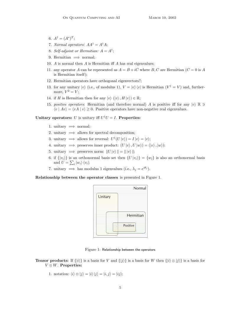
Relationship between the operator classes is presented in Figure 1.
1
Normal
Unitary
Hermitian
Positive
Figure 1: Relationship between the operators
Tensor products: If |i〉 is a basis for V and |j〉 is a basis for W then |i〉 ⊗ |j〉 is a basis forV ⊗W . Properties:
1. notation: |i〉 ⊗ |j〉 = |i〉 |j〉 = |i, j〉 = |ij〉;
5
March 10, 2002 Vadim Bulitko
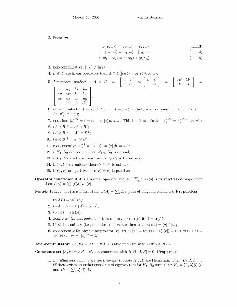
2. linearity:
z(|v, w〉) = |zv, w〉 = |v, zw〉 (1.1.13)|v1 + v2, w〉 = |v1, w〉+ |v2, w〉 (1.1.14)|v, w1 + w2〉 = |v, w1〉+ |v, w2〉 (1.1.15)
3. non-commutative: |vw〉 6= |wv〉;4. if A,B are linear operators then A⊗B(|vw〉) = A |v〉 ⊗A |w〉;
5. Kronecker product: A ⊗ B =[a bc d
]⊗
[x yv w
]=
[aB bBcB dB
]=
ax ay bx byav aw bv bwcx cy dx dycv cw dv dw
;
6. inner product: (|vw〉 , |v′w′〉) = (|v〉 , |v′〉) · (|w〉 , |w′〉) or simply: 〈vw | v′w′〉 =〈v | v′〉 〈w | w′〉;
7. notation: |v〉⊗k = (|v〉 ⊗ · · · ⊗ |v〉)k times. This is left associative: |v〉⊗k = |v〉⊗k−1 ⊗ |v〉 ?
8. (A⊗B)∗ = A∗ ⊗B∗;
9. (A⊗B)T = AT ⊗BT ;
10. (A⊗B)† = A† ⊗B†;
11. consequently: |ab〉† = |a〉† |b〉† = 〈a| 〈b| = 〈ab|;12. if N1, N2 are normal then N1 ⊗N2 is normal;
13. if H1,H2 are Hermitian then H1 ⊗H2 is Hermitian;
14. if U1, U2 are unitary then U1 ⊗ U2 is unitary;
15. if P1, P2 are positive then P1 ⊗ P2 is positive;
Operator functions: if A is a normal operator and A =∑
a a |a〉 〈a| is its spectral decompositionthen f(A) =
∑a f(a) |a〉 〈a|.
Matrix traces: if A is a matrix then tr(A) =∑
iAii (sum of diagonal elements). Properties:
1. tr(AB) = tr(BA);
2. tr(A+B) = tr(A) + tr(B);
3. tr(zA) = z tr(A);
4. similarity transformation: if U is unitary then tr(UAU†) = tr(A);
5. if |u〉 is a unitary (i.e., modulus of 1) vector then tr(A |u〉 〈u|) = 〈u|A |u〉;6. consequently for any unitary vector |v〉, tr(|v〉 〈v|) = tr(|v〉 〈v| |v〉 〈v|) = 〈v| (|v〉 〈v|) |v〉 =〈v | v〉 〈v | v〉 = | |v〉 |4 = 1.
Anti-commutator: A,B = AB +BA, A anti-commutes with B iff A,B = 0.
Commutator: [A,B] = AB −BA, A commutes with B iff [A,B] = 0. Properties:
1. Simultaneous diagonalization theorem: suppose H1,H2 are Hermitian. Then [H1,H2] = 0iff there exists an orthonormal set of eigenvectors for H1,H2 such that: H1 =
∑i λ
′i |i〉 〈i|
and H2 =∑
i λ′′i |i〉 〈i|;
6
On Quantum Computing and AI March 10, 2002
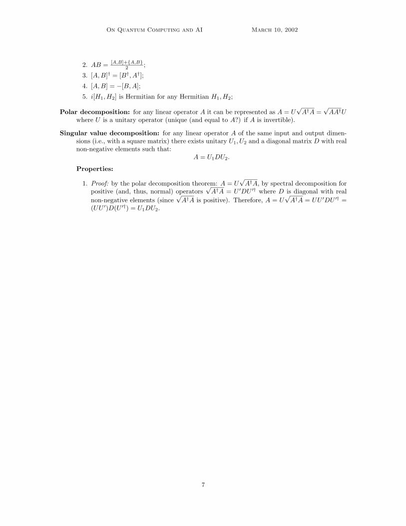
2. AB = [A,B]+A,B2 ;
3. [A,B]† = [B†, A†];
4. [A,B] = −[B,A];
5. i[H1,H2] is Hermitian for any Hermitian H1,H2;
Polar decomposition: for any linear operator A it can be represented as A = U√A†A =
√AA†U
where U is a unitary operator (unique (and equal to A?) if A is invertible).
Singular value decomposition: for any linear operator A of the same input and output dimen-sions (i.e., with a square matrix) there exists unitary U1, U2 and a diagonal matrix D with realnon-negative elements such that:
A = U1DU2.
Properties:
1. Proof: by the polar decomposition theorem: A = U√A†A, by spectral decomposition for
positive (and, thus, normal) operators√A†A = U ′DU ′† where D is diagonal with real
non-negative elements (since√A†A is positive). Therefore, A = U
√A†A = UU ′DU ′† =
(UU ′)D(U ′†) = U1DU2.
7
March 10, 2002 Vadim Bulitko
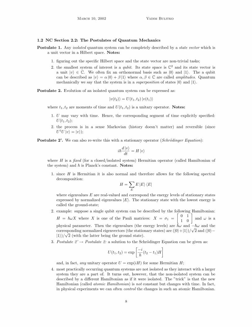
1.2 NC Section 2.2: The Postulates of Quantum Mechanics
Postulate 1. Any isolated quantum system can be completely described by a state vector which isa unit vector in a Hilbert space. Notes:
1. figuring out the specific Hilbert space and the state vector are non-trivial tasks;2. the smallest system of interest is a qubit. Its state space is C2 and its state vector is
a unit |v〉 ∈ C. We often fix an orthonormal basis such as |0〉 and |1〉. The a qubitcan be described as |v〉 = α |0〉 + β |1〉 where α, β ∈ C are called amplitudes. Quantummechanically we say that the system is in a superposition of states |0〉 and |1〉.
Postulate 2. Evolution of an isolated quantum system can be expressed as:
|v(t2)〉 = U(t1, t2) |v(t1)〉
where t1, t2 are moments of time and U(t1, t2) is a unitary operator. Notes:
1. U may vary with time. Hence, the corresponding segment of time explicitly specified:U(t1, t2);
2. the process is in a sense Markovian (history doesn’t matter) and reversible (sinceU†U |v〉 = |v〉);
Postulate 2’. We can also re-write this with a stationary operator (Schrodinger Equation):
i~d |v〉dt
= H |v〉
where H is a fixed (for a closed/isolated system) Hermitian operator (called Hamiltonian ofthe system) and ~ is Planck’s constant. Notes:
1. since H is Hermitian it is also normal and therefore allows for the following spectraldecomposition:
H =∑E
E |E〉 〈E|
where eigenvalues E are real-valued and correspond the energy levels of stationary statesexpressed by normalized eigenvalues |E〉. The stationary state with the lowest energy iscalled the ground-state;
2. example: suppose a single qubit system can be described by the following Hamiltonian:
H = ~ωX where X is one of the Pauli matrices: X = σ1 =[
0 11 0
]and ω is a
physical parameter. Then the eigenvalues (the energy levels) are ~ω and −~ω and thecorresponding normalized eigenvectors (the stationary states) are (|0〉+|1〉)/
√2 and (|0〉−
|1〉)/√
2 (with the latter being the ground state).3. Postulate 2’ → Postulate 2: a solution to the Schrodinger Equation can be given as:
U(t1, t2) = exp[−i~
(t2 − t1)H]
and, in fact, any unitary operator U = exp(iH) for some Hermitian H;4. most practically occurring quantum systems are not isolated as they interact with a larger
system they are a part of. It turns out, however, that the non-isolated system can bedescribed by a different Hamiltonian as if it were isolated. The ”trick” is that the newHamiltonian (called atomic Hamiltonian) is not constant but changes with time. In fact,in physical experiments we can often control the changes in such an atomic Hamiltonian.
8
On Quantum Computing and AI March 10, 2002
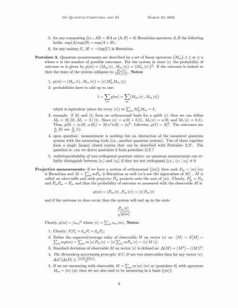
5. for any commuting (i.e., AB = BA or [A,B] = 0) Hermitian operators A,B the followingholds: exp(A) exp(B) = exp(A+B);
6. for any unitary U , H = −i log(U) is Hermitian.
Postulate 3. Quantum measurements are described by a set of linear operators Mm, 1 ≤ m ≤ nwhere n is the number of possible outcomes. For the system in state |v〉 the probability ofoutcome m is given by p(m) = (Mm |v〉 ,Mm |v〉) = ‖Mm |v〉 ‖2. If the outcome is indeed m
then the state of the system collapses to Mm|v〉‖Mm|v〉‖ . Notes:
1. p(m) = (Mm |v〉 ,Mm |v〉) = 〈v|M†mMm |v〉;
2. probabilities have to add up to one:
1 =∑m
p(m) =∑m
(Mm |v〉 ,Mm |v〉)
which is equivalent (since for every |v〉) to∑
mM†mMm = I;
3. example: if |0〉 and |1〉 form an orthonormal basis for a qubit |v〉 then we can defineM0 = |0〉 〈0| ,M1 = |1〉 〈1|. Since |v〉 = a |0〉 + b |1〉, M0 |v〉 = a |0〉 and M1 |v〉 = b |1〉.Thus, p(0) = (a |0〉 , a |0〉) = 〈0| a∗a |0〉 = |a|2. Likewise, p(1) = |b|2. The outcomes area|a| |0〉 xor b
|b| |1〉;
4. open question: measurement is nothing but an interaction of the measured quantumsystem with the measuring tools (i.e., another quantum system). Two of them togetherform a single [larger] closed system that can be described with Postulate 2/2’. Thequestion is: can we derive postulate 3 from postulate 2/2’?
5. indistinguishability of non-orthogonal quantum states: no quantum measurement can re-liably distinguish between |v1〉 and |v2〉 if they are not orthogonal (i.e., 〈v1 | v2〉 6= 0.
Projective measurements: if we have a system of orthonormal |m〉 then each Pm = |m〉 〈m|is Hermitian and M =
∑mmPm is Hermitian as well (m’s are the eigenvalues of M) . M is
called an observable and each projector Pm projects onto the axis of |m〉. Clearly, P †m = Pm
and PmPm = Pm and thus the probability of outcome m measured with the observable M is
p(m) = (Pm |v〉 , Pm |v〉) = 〈v|Pm |v〉
and if the outcome m does occur then the system will end up in the state
Pm |v〉√p(m)
.
Clearly, p(m) = |αm|2 where |v〉 =∑
m αm |m〉. Notes:
1. Clearly: PiPj = δijPi = δijPj ;
2. Define the expected/average value of observable M on vector |v〉 as: 〈M〉 = E[M ] =∑mmp(m) =
∑mm 〈v|Pm |v〉 = 〈v|
∑mmPm |v〉 = 〈v|M |v〉.
3. Standard deviation of observable M on vector |v〉 is defined as: ∆(M) =⟨M2
⟩− (〈M〉)2.
4. The Heisenberg uncertainty principle: if C,D are two observables then for any vector |v〉:∆(C)∆(D) ≥ |〈v|[C,D]|v〉|
2 .
5. If we are measuring with observable M =∑
mm |m〉 〈m| or (postulate 3) with operatorsMm = |m〉 〈m| then we are also said to be measuring in a basis |m〉.
9
March 10, 2002 Vadim Bulitko
6. Repeatability: if we measure with an observable M and get an outcome m then anothermeasurement with M will gives us m again. This is not true with many physical mea-surements indicating that they are not projective. This is also not true with general Mm
(postulate 3) since in general: M†m 6= Mm and MiMj 6= δijMj .
POVM measurements: given a general (postulate 3) system of measurement operators Mm wecan define POVM elements as Em = M†
mMm. Properties/notes:
1.∑
mEm = I (follows from∑
mM†mMm = I);
2. p(m) = 〈v|Em |v〉;3. Em are positive operators;
4. the resulting state (in the case of outcome m) is Mm|v〉√‖Mm|v〉‖
which is not easily expressible
with Em. So POVM elements are used when the resulting states are not important;
5. given a set of positive operators Em that satisfy the completeness relation (∑
mEm = I)we can define the general measurement operators as Mm =
√Em (therefore M†
mMm =Em).
6. projectors Pm = |m〉 〈m| comprise a special case of POVMs: Em = Pm would do.
7. phase: suppose we have a basis |i〉. Then any vector |v〉 has an amplitude αi whenrepresented in the basis: |v〉 =
∑i αi |i〉. We can associate phase factors θi ∈ R with each
|i〉. Then:
(a) relative phase difference: two states |v〉 and |w〉 differ by a relative phase θj in abasis |j〉 iff each |v〉’s amplitude αj differs by a relative phase θj from each |w〉’samplitude βj : αj = eiθjβj . The differences between |v〉 and |w〉 can be detected withappropriate measurement operators.
(b) global phase difference: occurs when all all amplitudes are shifted by eiθ (i.e., whenall θj are equal to θ). This cannot be detected by any measurement operator Mm
since 〈v| e−iθM†mMme
iθ |v〉 = 〈v|M†mMm |v〉.
(c) note: For any two orthonormal bases (|vi〉, |wi〉) the operator converting betweenthem (U |vi〉 = |wi〉) is indeed unitary and can be encoded as: U =
∑|vi〉 〈wi|.
HOWEVER, the difference between a vector expressed in one basis and in the othervector can be a relative phase shift and not necessarily a global phase shift.Example: suppose we are converting from basis |0〉 , |1〉 to |0〉 ,− |1〉. The unitaryoperator is simply U = |0〉 〈0| − |1〉 〈1|. So if we take an arbitrary vector |v〉 =
α |0〉 + β |1〉 then U |v〉 = α |0〉 − β |1〉. Thus, the vector[αβ
]in basis |0〉 , |1〉
and the vector[αβ
]in basis |0〉 ,− |1〉 are related through a relative phase shift
ei0, eiπ. In other words, there is no single θ such that α |0〉+β |1〉 = eiθ(α |0〉−β |1〉).
Postulate 4: Composite Systems: if a composite quantum system consists of n subsystem eachevolving in its Hilbert space Vi then the state of the entire system evolves in
⊗i Vi. Further-
more, if each subsystem is in a particular state |vi〉 then the state of the entire system is⊗
i vi.Notes:
1. motivation: assume super-position principle: if |v〉 and |w〉 are possible states of a systemthen for any α, β ∈ C such that |α|2 + |β|2 = 1 the linear combination α |v〉+β |w〉 is alsoa possible state. Then we can derive postulate 4 using the properties of tensor products.
10
On Quantum Computing and AI March 10, 2002
2. Bell/EPR states. Define:
|b00〉 =|00〉+ |11〉√
2(1.2.1)
|b01〉 =|00〉 − |11〉√
2(1.2.2)
|b10〉 =|10〉+ |01〉√
2(1.2.3)
|b11〉 =|01〉 − |10〉√
2(1.2.4)
It turns out that they form an orthonormal basis for two qubits. Furthermore, for anysingle qubit linear operator V the value of 〈bij |V ⊗I |bij〉 = constV for all i, j. Therefore,it is impossible to distinguish between Bell states by measuring only the first qubit†.It is, however, possible to distinguish between the Bell states reliably since they areorthonormal. Indeed, all one needs to do is to use a set of projective measurementoperators: Pij = |bij〉 〈bij |.
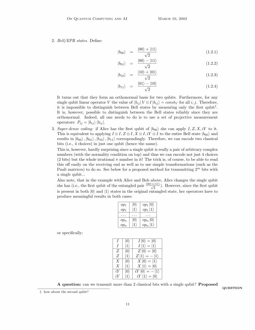
3. Super-dense coding: if Alice has the first qubit of |b00〉 she can apply I, Z,X, iY to it.This is equivalent to applying I ⊗ I, Z ⊗ I,X ⊗ I, iY ⊗ I to the entire Bell state |b00〉 andresults in |b00〉 , |b01〉 , |b10〉 , |b11〉 correspondingly. Therefore, we can encode two classicalbits (i.e., 4 choices) in just one qubit (hence the name).This is, however, hardly surprising since a single qubit is really a pair of arbitrary complexnumbers (with the normality condition on top) and thus we can encode not just 4 choices(2 bits) but the whole irrational π number in it! The trick is, of course, to be able to readthis off easily on the receiving end as well as to use simple transformations (such as thePauli matrices) to do so. See below for a proposed method for transmitting 2m bits witha single qubit...Also note, that in the example with Alice and Bob above, Alice changes the single qubitshe has (i.e., the first qubit of the entangled pair |00〉+|11〉√
2). However, since the first qubit
is present in both |0〉 and |1〉 states in the original entangled state, her operators have toproduce meaningful results in both cases:
op1 |0〉 op1 |0〉op1 |1〉 op1 |1〉. . . . . . . . .opn |0〉 opn |0〉opn |1〉 opn |1〉
or specifically:
I |0〉 I |0〉 = |0〉I |1〉 I |1〉 = |1〉Z |0〉 Z |0〉 = |0〉Z |1〉 Z |1〉 = − |1〉X |0〉 X |0〉 = |1〉X |1〉 X |1〉 = |0〉iY |0〉 iY |0〉 = − |1〉iY |1〉 iY |1〉 = |0〉
A question: can we transmit more than 2 classical bits with a single qubit? ProposedQUESTION
†. how about the second qubit?
11
March 10, 2002 Vadim Bulitko
method: to transmit 2m classical bits prepare an entangled state of m qubits. Give thelast m−1 of them (|q2 . . . qm〉) to Bob and the first one (|q1〉) to Alice. Then Alice appliesone of her 2m linear operators (the one with the index 1 ≤ i ≤ 2m where i is the classicalmessage she is transmitting) on |q1〉 and sends the result to Bob. This is equivalent toapplying opi ⊗ I ⊗ · · · ⊗ I on the initial entangled state. Let’s call the resulting m-qubitstate |bi〉 (1 ≤ i ≤ 2m). The only requirement is that |b1〉 , . . . , |b2m〉 are orthonormaland therefore can be reliably distinguished (e.g., with the observableM =
∑2m
i=1 i |bi〉 〈bi|).4. Entanglement, correlation, and anti-correlation:
(a) Bell states in H2 have components (for each qubit) that project both on |0〉 and |1〉.Therefore, measuring either qubit in the basis |0〉 , |1〉 gives |0〉 with the probability1/2 and |1〉 with the probability 1/2. In other words:
〈bij | |0〉 〈0| |bij〉 =12
(1.2.5)
〈bij | |1〉 〈1| |bij〉 =12. (1.2.6)
So, if we measure the first qubit of any |bij〉 with say the observable M = α |0〉 〈0|+β |1〉 〈1| then we get α in half cases and β in half cases (i.e., p(α) = p(β) = 1
2 ). Sup-pose, we make a measurement and get α. Then if the original Bell state was |0x〉±|1y〉√
2
then the resulting state collapses to |0x〉 (the 1√2
is removed by the normalization).Therefore, now if we measure the second qubit we are bound to see |x〉. So if |x〉 hap-pens to be |0〉 we will get correlation (the second qubit measurement is bound to givethe same result as the first qubit measurement) or (if |x〉 = |1〉) anti-correlation (thesecond qubit measurement is bound to be opposite to the first qubit measurement).
(b) Generally speaking, we want two properties here:i. the first measurement (of any qubit) can give us either |0〉 or |1〉 equally likely;ii. the second measurement (of the other qubit) gives us the result deterministically
dependant on the first measurement (i.e., correlation or anti-correlation).Hypothesis: this cannot be accomplished with a non-entangled state. Example: sup-
HYPOTHESIS pose we have non-entangled |v〉 = (a |0〉 + b |1〉)(c |0〉 + d |1〉). Then depending ona, b, c, d we will get two cases:i. one of the qubits in |v〉 is the same (e.g., |v〉 = (|0〉 + |1〉) |0〉 = |00〉 + |10〉 and
the measurement on the 2nd qubit always gives |0〉);ii. there are elements in the sum that start/end with the same qubit but end/start
with different ones (e.g., |v〉 = (|0〉+ |1〉)2 = |00〉+ |01〉+ |10〉+ |11〉 and no matterwhat we measure first the second measurement will be non-deterministic).
5. Bell inequalities. Suppose we have two particles: one in the possession of Alice and one inthe possession of Bob. Suppose Alice and Bob take measurements (outside of the null coneso that one doesn’t affect the other) of two quantities each: Q = ±1, R = ±1;S = ±1, T =±1. Consider, the quantity: QS+RS+RT−QT = (Q+R)S+(R−Q)T = ±2. Suppose,there is a state of the system and it is Q = q,R = r, S = s, T = t with the probability ofp(q, r, s, t) before the measurement. The expected value is: E(QS+RS+RT −QT ) ≤ 2.On the other hand, E(QS + RS + RT − QT ) = E(QS) + E(RS) + E(RT ) − E(QT ).Thus, the Bell inequality is E(QS) + E(RS) + E(RT )− E(QT ) ≤ 2.
Quantum mechanically, however, we can take |b11〉 = |01〉−|10〉√2
and measure the following
observables: Q = Z1, R = X1, S = −Z2−X2√2
, T = Z2−X2√2
. On the entangled state |b11〉their expected values are: 〈QS〉 = 1√
2, 〈RS〉 = 1√
2, 〈RT 〉 = 1√
2, 〈QT 〉 = − 1√
2and,
12
On Quantum Computing and AI March 10, 2002
therefore, the expected value of the entire quantity is: 〈QS〉 + 〈RS〉 + 〈RT 〉 − 〈QT 〉 =2√
2 > 2!Experiments show that Nature follows the second way and the measured value of theobservables is greater than 2. This means that at least one of the following assumptionsdoesn’t hold:
(a) realism: Q,R, S, T have values independent of observation;(b) locality: Alice’s measurement doesn’t affect Bob’s measurement.
Note that the same trick doesn’t work with a non-entangled state such as |00〉 whichresults in 〈QS〉 = − 1√
2, 〈RS〉 = 0, 〈RT 〉 = 0, 〈QT 〉 = 1√
2and, therefore, the expected
value of the entire quantity is: 〈QS〉+ 〈RS〉+ 〈RT 〉 − 〈QT 〉 = −√
2 < 2.
1.3 NC 3.1.2: Circuits
Universality: the following gates seem to be needed:
1. Auxilary gates: wires + ancilla bits + fanout + crossover;arethecrossover/ancillabitsre-allyneeded?
2. NAND / AND+NOT / XOR;
1.4 NC 3.2: Computational Complexity
Complexity classes can be defined as follows:
L (logarithmic space) is the class of languages that can be decided by a deterministic TMrunning in O(log(n)) space (the restriction applies to the working tape only);
P (polynomial time) is the class of languages that can be decided by a deterministic TMrunning in O(nk) time;
NP (non-deterministic polynomial time) is the class of languages that can be verified bya deterministic TM running O(nk) time. More technically: L ∈ NP if ∃M∃k∀`[(` ∈L =⇒ ∃wM(`, w) = 1 in O(|`|k)) & (` 6∈ L =⇒ ∀wM(`, w) = 0 in O(|`|k))]. Inother words, we require a witness w for each positive (i.e., ` ∈ L) instance. Example:L = ` ∈ N|` is not prime ∈ NP .
coNP is the class of languages where we require a witness for every negative (i.e., ` 6∈ L)instance. Clearly, ∀L[L ∈ NP ⇐⇒ L ∈ coNP ]. Example: L = ` ∈ N|` is prime ∈coNP .
NP -complete is the class of languages from NP such that for any language L from NP Lcan be polynomially reduced to that NP -complete language;
NPI (NP intermediate) is the class of languages that are NP but not NP -complete;
PSPACE (polynomial space) is the class of languages that can be decided in polynomialspace by a deterministic TM;
EXP (exponential time) is the class of languages that can be decided by a deterministic TMrunning in O(2nk
) time;
Notes:
1. TIME(f(n)) ⊂ TIME(f(n) log2(f(n))) (the time hierarchy theorem);
2. SPACE(f(n)) ⊂ SPACE(f(n) log(f(n))) (the space hierarchy theorem);
3. P ⊂ EXP ;
4. L ⊂ PSPACE ;
13
March 10, 2002 Vadim Bulitko
5. L ⊆ P ⊆ NP ⊆ PSPACE ⊆ EXP ;
6. factoring is not proven to be NP -complete and is suspected to be NPI ;
7. graph isomorphism is not proven to be NP -complete and is suspected to be NPI ;
Quantum computational power is currently believed (but not proven) to be higher than thatof conventional computing devices insomuch as:
1. Polynomial quantum algorithms are known to be in PSPACE ;
2. QC are believed to be able to do NPI problems in polynomial time but not NP -completetasks.
1.5 NC 3.2.5: Energy and reversibility
Landauer’s principle: any time a bit of information is erased an amount of energy dissipated intothe environment is lower bounded by kBT ln 2. Alternatively, the entropy goes up by at leastkBT ln 2. Notes:
1. I think the intuition here is that erasing information makes things more uniform (since itreduces a certain [unknown/chaotic] state to a known brand-new erased state. Therefore,the amount of order increases raising the entropy.
2. Reversible computations can be theoretically carried out with no energy used! However,in practice, noise correction requires keeping track of errors, and, therefore, erasing thesetemporary working records. Thus, in practice one needs to dissipate energy while com-puting.
Fredkin Gate is a universal reversible gate. It has two data (A,B) and one control (C) input andoutputs (A′, B′, C ′). In other words, F (A,B,C) = (A′, B′, C ′). The control always passesthrough unchanged: C ′ = C while the gate swaps A,B if C = 1 and passes them straightotherwise. Notes:
1. F (0, y, x) = (xy, xy, x) (and);
2. F (1, 0, x) = (x, x, x) (not, fanout);
3. F (x, y, 1) = (y, x, 1) (cross-over);
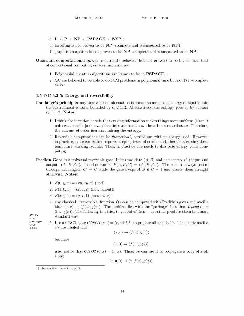
4. any classical [irreversible] function f() can be computed with Fredkin’s gates and ancillabits: (x, a) → (f(x), g(x)). The problem lies with the ”garbage” bits that depend on x(i.e., g(x)). The following is a trick to get rid of them – or rather produce them in a more
WHYaregarbagebitsbad?
standard way.
5. Use a CNOT-gate (CNOT (c, t) = (c, c⊕ t)‡) to prepare all ancilla 1’s. Thus, only ancilla0’s are needed and
(x, a) → (f(x), g(x))
becomes(x, 0) → (f(x), g(x)).
Also notice that CNOT (0, x) = (x, x). Thus, we can use it to propagate a copy of x allalong
(x, 0, 0) → (x, f(x), g(x)).
‡. here a ⊕ b = a + b mod 2.
14
On Quantum Computing and AI March 10, 2002
6. We now add a forth register that starts in a random state y: (x, 0, 0, y). We computef(x) using Fredkin’s gates and add it modulo 2 with the y:
(x, 0, 0, y) U1→ (x, f(x), g(x), y) U2→ (x, f(x), g(x), y ⊕ f(x)).
Since U1 is reversible and didn’t touch y we can undo it (called uncomputation):
(x, f(x), g(x), y ⊕ f(x))(U1)
−1
−→ (x, 0, 0, y ⊕ f(x)).
Dropping 0’s we get(x, y) → (x, y ⊕ f(x)).
This is reversible and there are no garbage bits depending on x.???⊕f(x)???7. The overhead of making a computation reversible is a constant factor and thus P and
NP classes don’t change.
Toffoli gate is defined as T (A,B,C) = (A,B,C ⊕AB). Notes:Crossover?
1. T (x, y, 1) = (x, y, xy) (nand);
2. T (x, y, 0) = (x, y, xy) (and);
3. T (x, 1, 0) = (x, 1, x) (fanout);
4. T (1, 1, x) = (1, 1, x) (not);
5. Toffoli → Fredkin: 9 Fredkin gates are enough to simulate a Toffoli gate. Is this theminimum?
6. Fredkin → Toffoli: 15 Toffoli gates are enough to simulate a Fredkin gate. Is this theminimum?
15
On Quantum Computing and AI March 10, 2002
References
[Bulitko et al. 2002] Bulitko, V., Levner, I., Greiner, R. (2002). State Abstraction and Lookahead Con-trol Policies. In Proceedings of the American Association for Artificial Intelligence(AAAI) Conference. AAAI Press. (submitted)
[Korf 1990] Korf, R.E. (1990). Real-time heuristic search. Artificial Intelligence, Vol. 42, No. 2-3,pp. 189-211.
[Mitchell 1997] Mitchell, T. (1997). Machine Learning. WCB/McGraw-Hill.
[Nielsen et al. 2000] Nielsen, M., Chuang, L., (2000). Quantum Computation and Quantum Information.Cambridge University Press.
19
1
Quantum Computing Summer School
Lecture 2: Linear AlgebraLecture 2: Linear AlgebraAngela AntoniuAngela Antoniu
Department of Electrical and Department of Electrical and Computing EngineeringComputing Engineering
May 7, 2002May 7, 2002
Introduction to Quantum Introduction to Quantum MechanicsMechanics
Chapter objective (lectures 2,3,4):Chapter objective (lectures 2,3,4):To introduce all of the fundamental principles of To introduce all of the fundamental principles of Quantum mechanicsQuantum mechanics
Quantum mechanics Quantum mechanics The most realistic known description of the worldThe most realistic known description of the worldThe basis for quantum computing and quantum The basis for quantum computing and quantum informationinformation
Why Linear Algebra?Why Linear Algebra?L A is the prerequisite for understanding Quantum L A is the prerequisite for understanding Quantum MechanicsMechanics
What is Linear Algebra?What is Linear Algebra?… is the study of vector spaces… and of… is the study of vector spaces… and of
linear operations on those vector spaces1]linear operations on those vector spaces1]
2
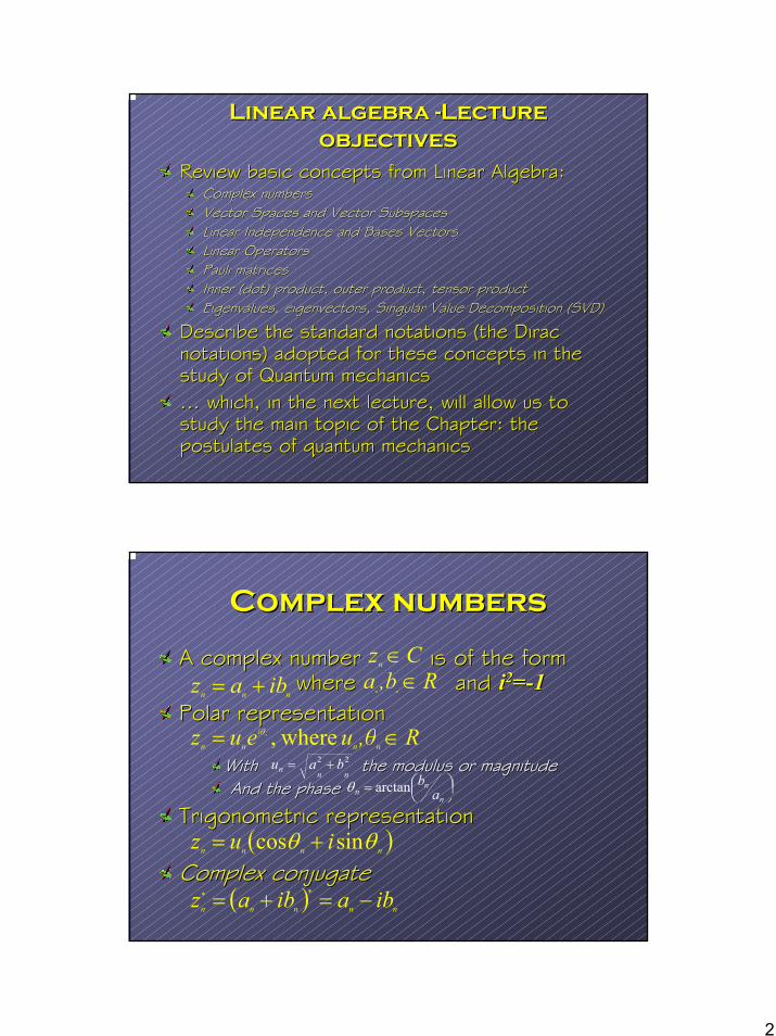
Linear algebra Linear algebra --Lecture Lecture objectivesobjectives
Review basic concepts from Linear Algebra:Review basic concepts from Linear Algebra:Complex numbersComplex numbersVector Spaces and Vector SubspacesVector Spaces and Vector SubspacesLinear Independence and Bases VectorsLinear Independence and Bases VectorsLinear OperatorsLinear OperatorsPauli matrices Pauli matrices Inner (dot) product, outer product, tensor productInner (dot) product, outer product, tensor productEigenvalues, eigenvectors, Singular Value Decomposition (SVD)Eigenvalues, eigenvectors, Singular Value Decomposition (SVD)
Describe the standard notations (the Dirac Describe the standard notations (the Dirac notations) adopted for these concepts in the notations) adopted for these concepts in the study of Quantum mechanicsstudy of Quantum mechanics… which, in the next lecture, will allow us to … which, in the next lecture, will allow us to study the main topic of the Chapter: the study the main topic of the Chapter: the postulates of quantum mechanicspostulates of quantum mechanics
Complex numbersComplex numbers
A complex numberA complex number isis of the form of the form where where and and ii22==--11
Polar representationPolar representation
With the modulus or magnitudeWith the modulus or magnitudeAnd the phaseAnd the phase
Trigonometric representationTrigonometric representation
Complex conjugateComplex conjugate
nnn ibaz += R ,bann∈Czn ∈
where, R,θueuz nn
i
nnn ∈= θ
22
nnn bau +=
=
nn
n abarctanθ
( )nnnn iuz θθ sincos +=
( ) nnnnn ibaibaz −=+= ∗∗
3
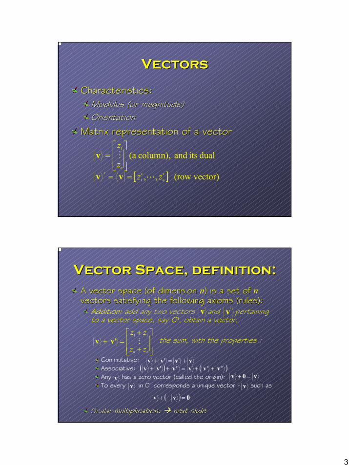
VectorsVectors
Characteristics:Characteristics:Modulus (or magnitude)Modulus (or magnitude)Orientation Orientation
Matrix representation of a vectorMatrix representation of a vector
[ ] vector)(row ,,
dual its and column), (a
1
1
∗∗==
=
n
n
zzz
z
L
M
vv
v
τ
Vector Space, definition:Vector Space, definition:A vector space (of dimension A vector space (of dimension n) is a set of ) is a set of nvectors satisfying the following axioms (rules):vectors satisfying the following axioms (rules):
Addition: add any two vectors and pertaining to a vector space, say Cn, obtain a vector,
the sum, with the properties :
Commutative: Associative:Any has a zero vector (called the origin): To every in Cn corresponds a unique vector - such as
Scalar Scalar multiplication: multiplication: next slidenext slide
v 'v
+
+=+
'
'11
'nn zz
zzMvv
vvvv +=+ ''( ) ( )'''''' vvvvvv ++=++
v0v =+vv v
( ) 0vv =−+
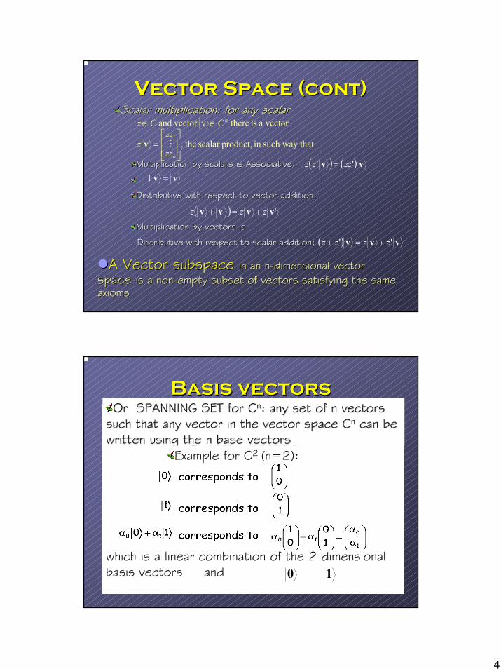
4
Vector Space (cont)Vector Space (cont)Scalar Scalar multiplication: for any scalar multiplication: for any scalar
Multiplication by scalars is Associative:Multiplication by scalars is Associative:
Distributive with respect to vector addition: Distributive with respect to vector addition:
Multiplication by vectors isMultiplication by vectors is
Distributive with respect to scalar addition:Distributive with respect to scalar addition:
A Vector subspaceA Vector subspace in an nin an n--dimensional vectordimensional vectorspace space is a nonis a non--empty subset of vectors satisfying the same empty subset of vectors satisfying the same axiomsaxioms
hat such way tin product,scalar the,
vectora is therev vector and 1
=
∈∈
n
n
zz
zzz
CCz
Mv
( ) ( ) vv '' zzzz =vv =1
( ) '' vvvv zzz +=+
( ) vvv '' zzzz +=+
Basis vectorsBasis vectorsOr SPANNING SET for Or SPANNING SET for CCnn: any set of n vectors : any set of n vectors
such that any vector in the vector space such that any vector in the vector space CCnn can be can be written using the n base vectors written using the n base vectors
Example for C2 (n=2):
which is a linear combination of the 2 dimensional basis vectors and 0 1
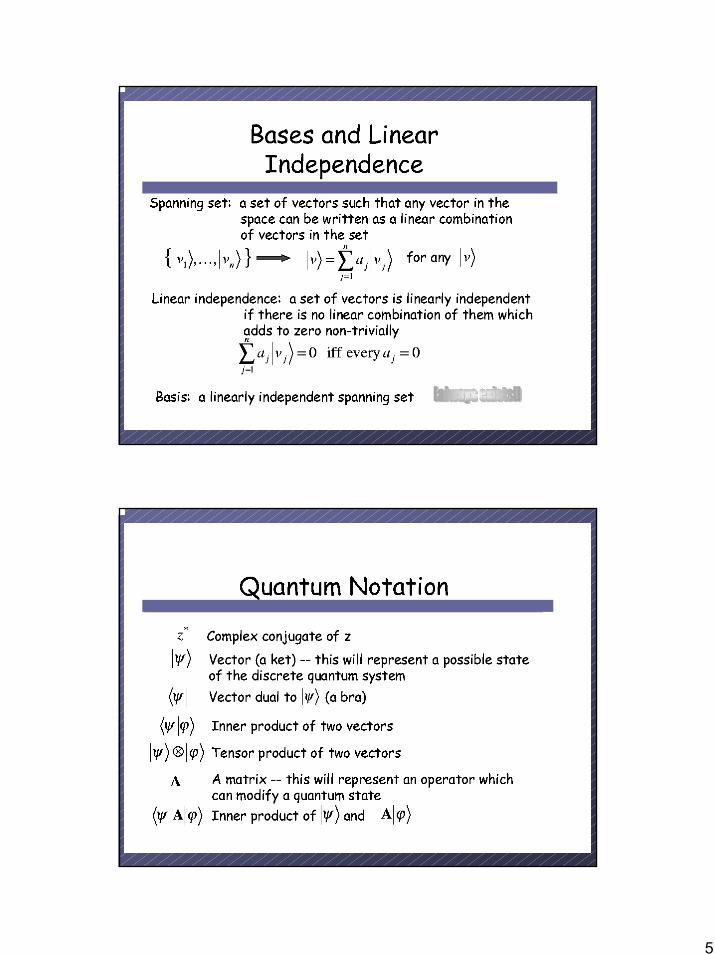
5
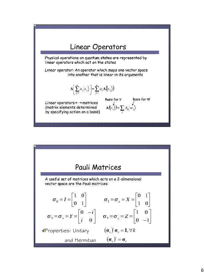
6
Properties: Unitary
and Hermitian
( ) kkk ∀= ,Iσσ τ
( ) kk σσ =τ
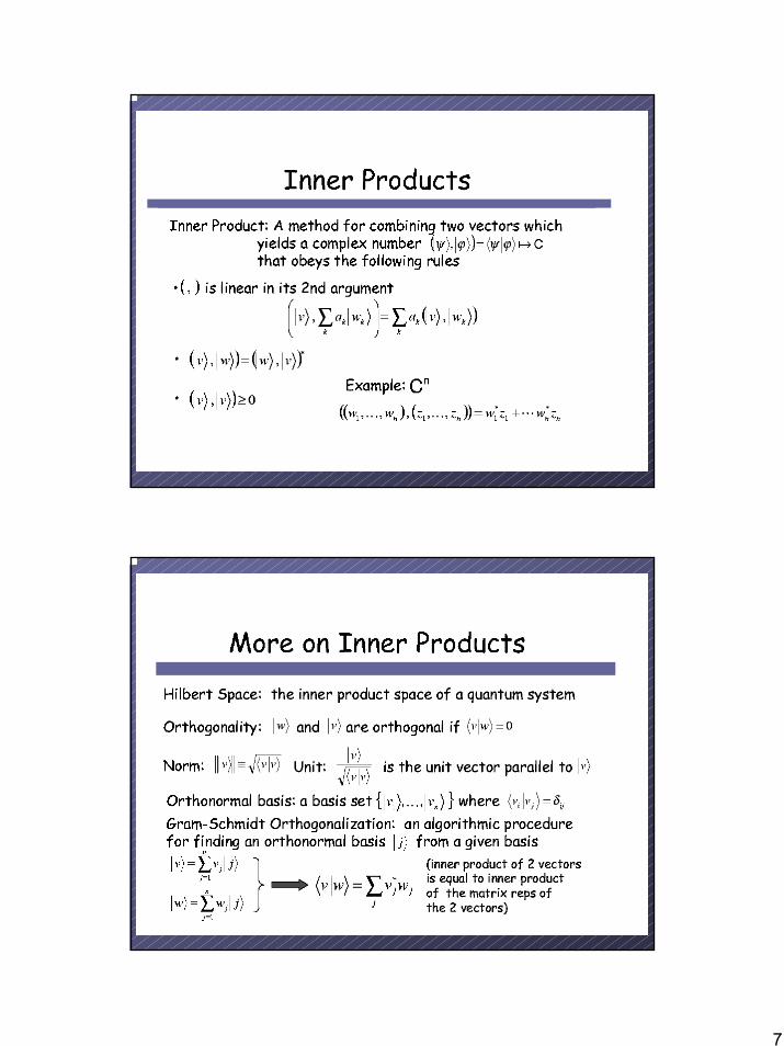
7
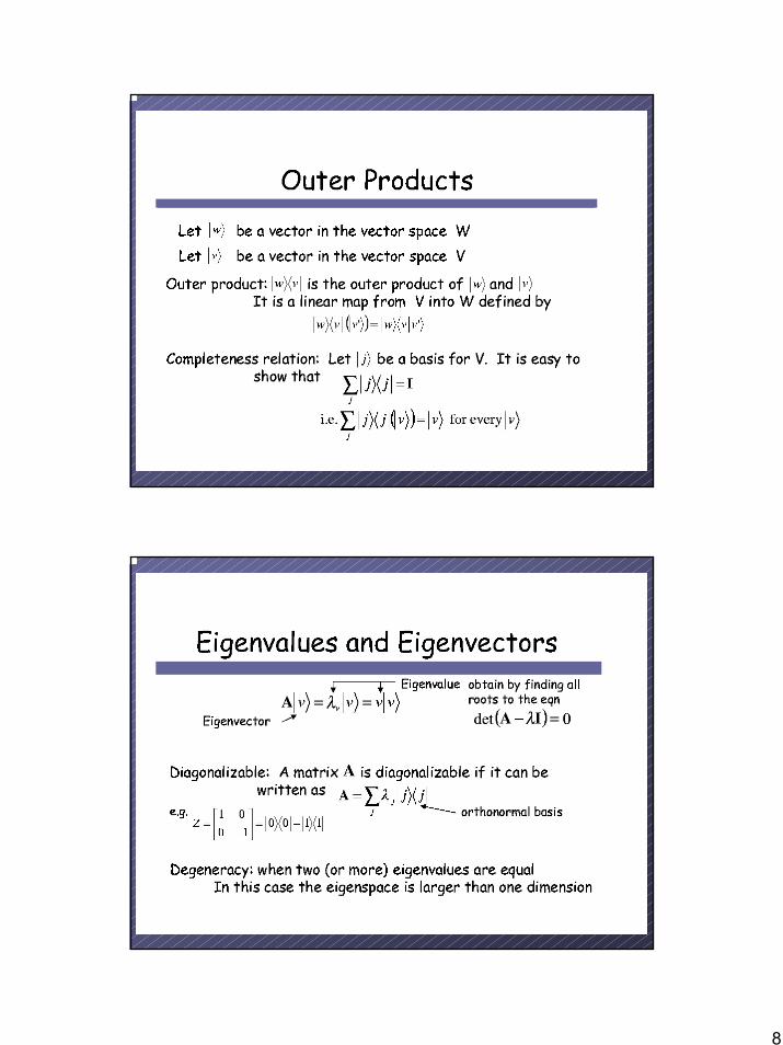
8
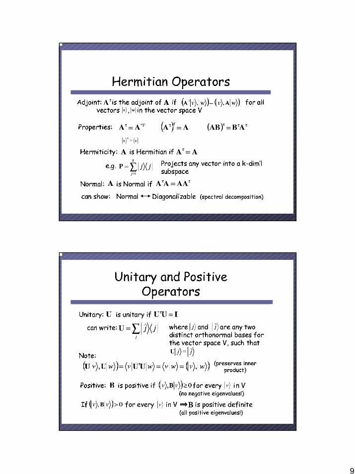
9
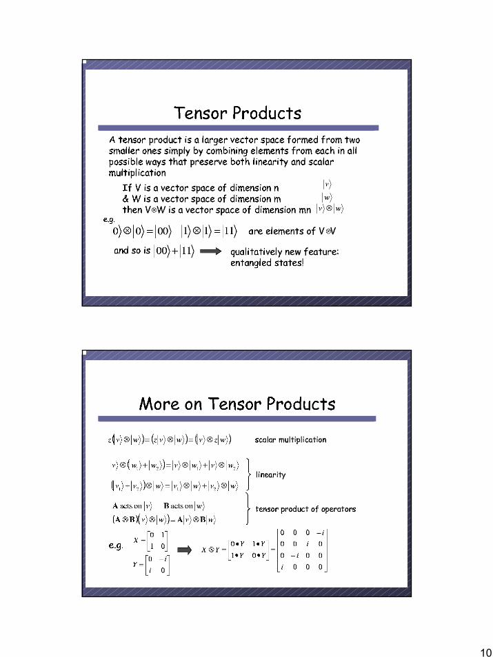
10
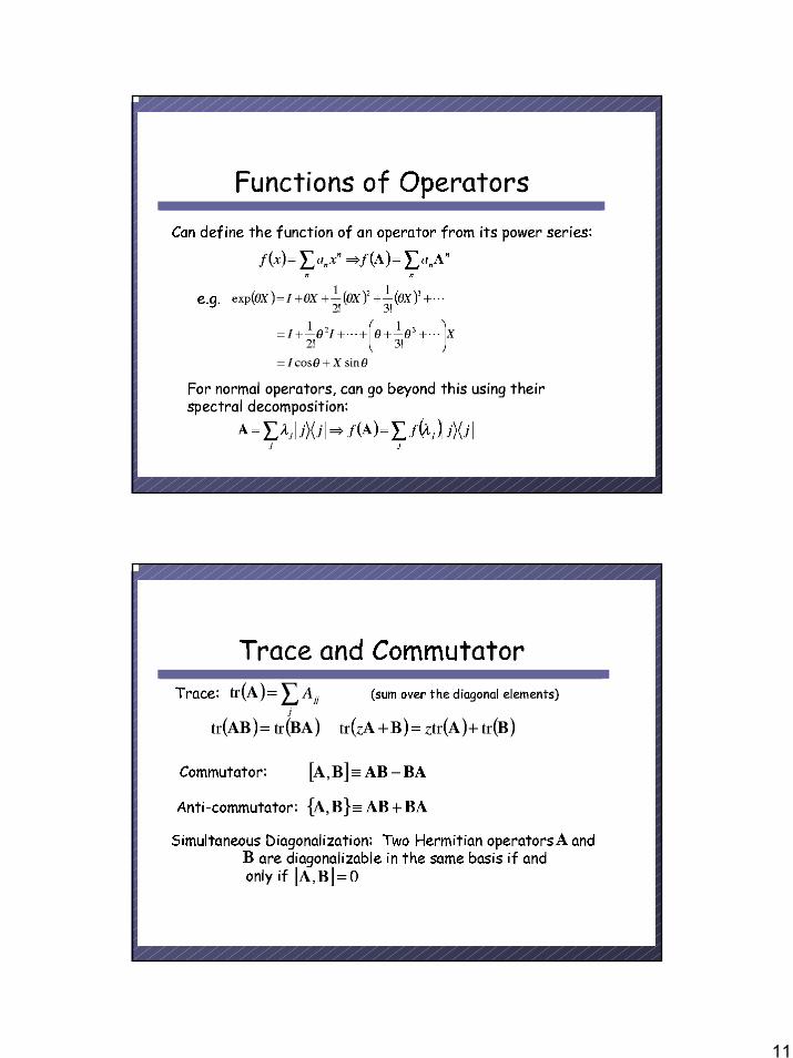
11
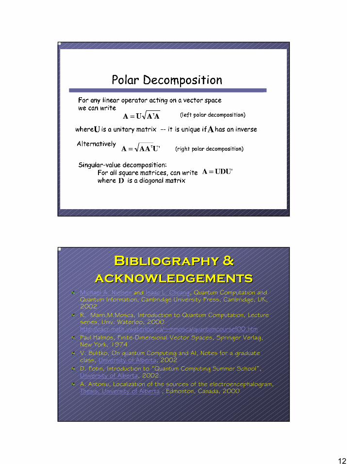
12
Bibliography & Bibliography & acknowledgementsacknowledgements
Michael A. Nielsen and Isaac L. Chuang, Quantum Computation and Quantum Information, Cambridge University Press, Cambridge, UK, 2002 R. Mann,M.Mosca, Introduction to Quantum Computation, Lecture series, Univ. Waterloo, 2000 http://cacr.math.uwaterloo.ca/~mmosca/quantumcoursef00.htmPaul Halmos, Finite-Dimensional Vector Spaces, Springer Verlag, New York, 1974V. Bulitko, On quantum Computing and AI, Notes for a graduate class, University of Alberta, 2002D. Fotin, Introduction to “Quantum Computing Summer School”, University of Alberta, 2002. A. Antoniu, Localization of the sources of the electroencephalogram, Thesis, University of Alberta , Edmonton, Canada, 2000
Qu
an
tu
m C
om
pu
tin
g
Su
mm
er
Sc
ho
ol
Lect
ure
4:
Lect
ure
4:
Sup
erSup
er-- D
ense
Cod
ing,
EPR
Den
se C
odin
g, E
PR
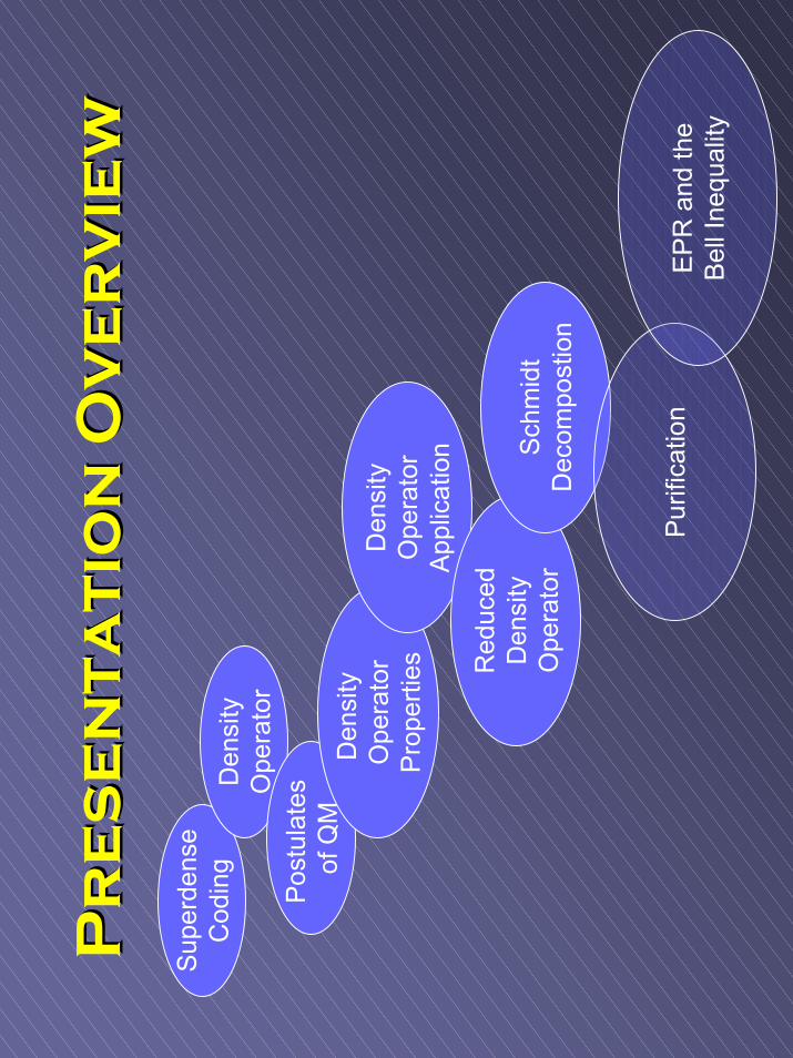
Pr
es
en
ta
tio
n O
ve
rv
iew
Pr
es
en
ta
tio
n O
ve
rv
iew
Supe
rden
seC
odin
gD
ensi
tyO
pera
tor
Post
ulat
es
of Q
MD
ensi
ty
Ope
rato
rPr
oper
ties
Den
sity
Ope
rato
rAp
plic
atio
nR
educ
edD
ensi
tyO
pera
tor
Schm
idt
Dec
ompo
stio
n
Purif
icat
ion
EPR
and
the
Bell
Ineq
ualit
y
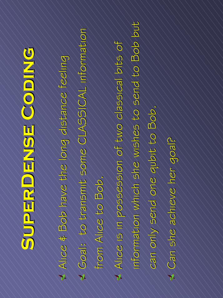
Su
pe
rD
en
se
Su
pe
rD
en
se
Co
din
gC
od
ing
Alic
e &
Bob
hav
e th
e lo
ng d
ista
nce
feel
ing
Alic
e &
Bob
hav
e th
e lo
ng d
ista
nce
feel
ing
Goa
l: t
o tr
ansm
it so
me
CLA
SSIC
AL
info
rmat
ion
Goa
l: t
o tr
ansm
it so
me
CLA
SSIC
AL
info
rmat
ion
from
Alic
e to
Bob
.from
Alic
e to
Bob
.
Alic
e is
in p
osse
ssio
n of
two
clas
sica
l bits
of
Alic
e is
in p
osse
ssio
n of
two
clas
sica
l bits
of
info
rmat
ion
whi
ch s
he w
ishe
s to
sen
d to
Bob
but
in
form
atio
n whi
ch s
he w
ishe
s to
sen
d to
Bob
but
ca
n on
ly s
end
one
can
only
sen
d on
e qu
bit
qubi
tto
Bob
.to
Bob
.
Can
she
ach
ieve
her
goa
l?
Can
she
ach
ieve
her
goa
l?
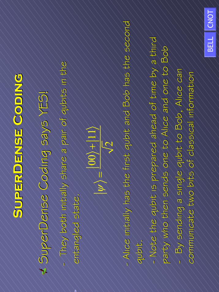
Su
pe
rD
en
se
Su
pe
rD
en
se
Co
din
gC
od
ing
Sup
erD
ense
Sup
erD
ense
Cod
ing
says
YES
!Cod
ing
says
YES
!--
They
bot
h in
itial
ly s
hare
a p
air
of
They
bot
h in
itial
ly s
hare
a p
air
of q
ubits
qubi
tsin
the
in
the
en
tang
led
stat
e.en
tang
led
stat
e.
--Alic
e in
itial
ly h
as t
he firs
t Alic
e in
itial
ly h
as t
he firs
t qu
bit
qubi
tan
d Bob
has
the
sec
ond
and
Bob
has
the
sec
ond
qubi
tqu
bit ..
--Not
e th
e Not
e th
e qu
bit
qubi
tis
pre
pare
d ah
ead
of t
ime
by a
thi
rd
is p
repa
red
ahea
d of
tim
e by
a t
hird
pa
rty
who
the
n se
nds
one
to A
lice
and
one
to B
obpa
rty
who
the
n se
nds
one
to A
lice
and
one
to B
ob--
By
send
ing
a si
ngle
By
send
ing
a si
ngle
qub
itqu
bit
to B
ob,
Alic
e ca
n to
Bob
, Alic
e ca
n co
mm
unic
ate
two
bits
of cl
assi
cal i
nfor
mat
ion
0011 2
ψ+
=
com
mun
icat
e tw
o bi
ts o
f cl
assi
cal i
nfor
mat
ion
BELL
CNO
T
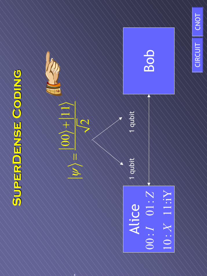
Su
pe
rD
en
se
Su
pe
rD
en
se
Co
din
gC
od
ing
0011 2
ψ+
=
Alic
e00
:
01:
10:
11:
iYI
ZX
Bob
1 qu
bit
1 qu
bit
CIRC
UIT
CNO
T
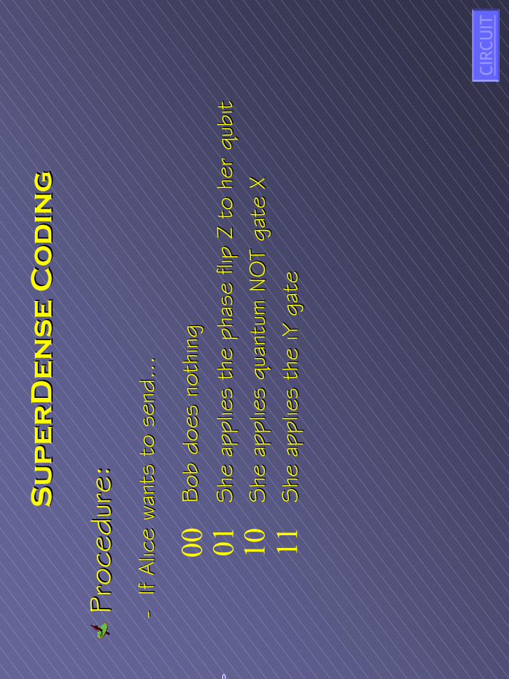
Su
pe
rD
en
se
Su
pe
rD
en
se
Co
din
gC
od
ing
Proc
edur
e:Pr
oced
ure:
--If
Alic
e wan
ts t
o se
nd…
If Alic
e wan
ts t
o se
nd…
Bob
doe
s no
thin
gBob
doe
s no
thin
g
She
app
lies
the
phas
e fli
p Z
to h
er
She
app
lies
the
phas
e fli
p Z
to h
er q
ubit
qubi
tShe
app
lies
quan
tum
NO
T ga
te X
She
app
lies
quan
tum
NO
T ga
te X
She
app
lies
the
She
app
lies
the
iYiYga
tega
te
00 01 10 11
CIRC
UIT
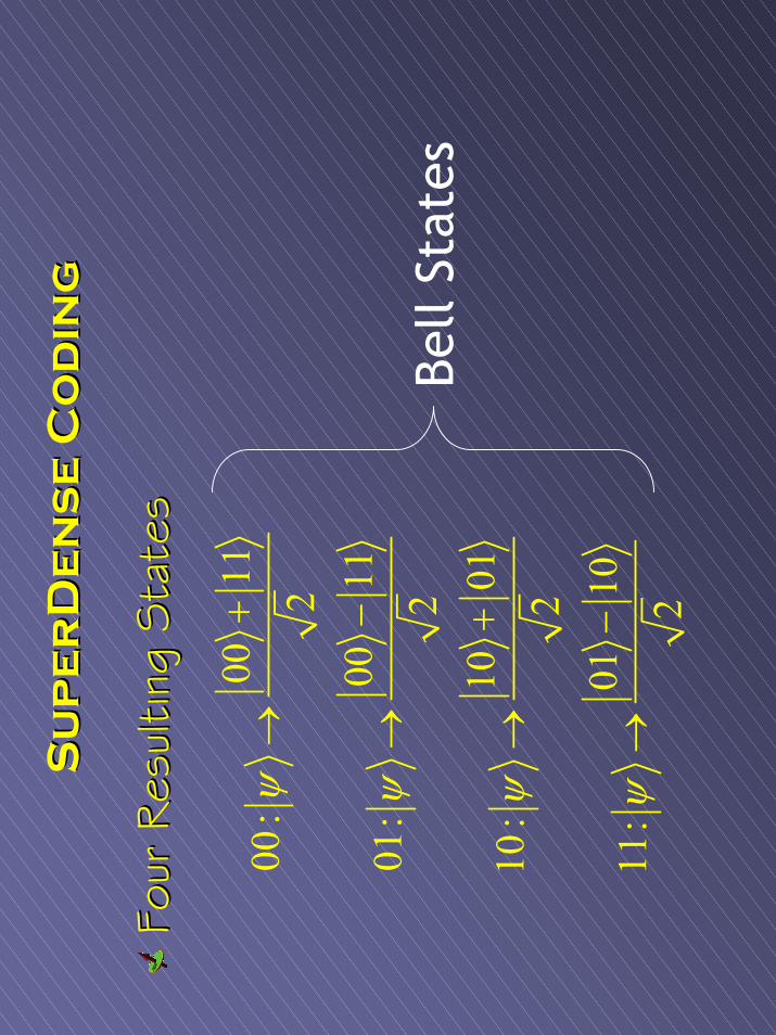
Su
pe
rD
en
se
Su
pe
rD
en
se
Co
din
gC
od
ing
Four
Res
ultin
g Sta
tes
Four
Res
ultin
g Sta
tes
0011
00:
200
1101
:2
1001
10:
201
1011
:2
ψ ψ ψ ψ
+→
−→
+→
−→
Bell
Stat
es
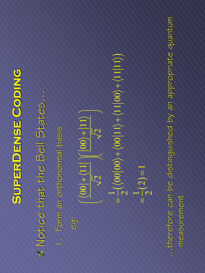
Su
pe
rD
en
se
Su
pe
rD
en
se
Co
din
gC
od
ing
Not
ice
that
the
Bel
l Sta
tes…
Not
ice
that
the
Bel
l Sta
tes…
1.
For
m a
n 1
. F
orm
an
orth
onor
mal
orth
onor
mal
basi
sba
sis
egeg::
…th
eref
ore
can
be d
istin
guis
hed
by a
n ap
prop
riate
qua
ntum
…
ther
efor
e ca
n be
dis
tingu
ishe
d by
an
appr
opria
te q
uant
um
mea
sure
men
t
()
()
0011
0011
22
100
0000
1111
0011
112 1
21
2
+
+
=+
++
==
mea
sure
men
t
De
ns
ity
Op
er
at
or
De
ns
ity
Op
er
at
or
--W
e ha
ve for
mul
ated
qua
ntum
mec
hani
cs u
sing
the
W
e ha
ve for
mul
ated
qua
ntum
mec
hani
cs u
sing
the
la
ngua
ge o
f th
e st
ate
vect
or.
lang
uage
of th
e st
ate
vect
or.
--Alte
rnat
ive
form
ulat
ion
is a
too
l cal
led
the
Alte
rnat
ive
form
ulat
ion
is a
too
l cal
led
the
DEN
SIT
Y O
PERATO
R o
r D
ENSIT
Y M
ATR
IXD
ENSIT
Y O
PERATO
R o
r D
ENSIT
Y M
ATR
IX
--M
athe
mat
ical
ly e
quival
ent
but
mor
e co
nven
ient
for
M
athe
mat
ical
ly e
quival
ent
but
mor
e co
nven
ient
for
th
inking
abo
ut s
ome
com
mon
qua
ntum
mec
hani
cs
thin
king
abo
ut s
ome
com
mon
qua
ntum
mec
hani
cs
scen
ario
ssc
enar
ios
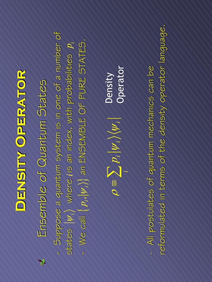
De
ns
ity
Op
er
at
or
De
ns
ity
Op
er
at
or
Ense
mbl
e of
Qua
ntum
Sta
tes
Ense
mbl
e of
Qua
ntum
Sta
tes
--Sup
pose
a q
uant
um s
yste
m is
in o
ne o
f a
num
ber
of
Sup
pose
a q
uant
um s
yste
m is
in o
ne o
f a
num
ber
of
stat
es
whe
re
is a
n in
dex,
with
pro
babi
litie
sst
ates
whe
re
is a
n in
dex,
with
pro
babi
litie
s--
We
call
an
ENSEM
BLE
OF
PURE
STA
TES.
We
call
an
ENSEM
BLE
OF
PURE
STA
TES.
--All
post
ulat
es o
f qu
antu
m m
echa
nics
can
be
All
post
ulat
es o
f qu
antu
m m
echa
nics
can
be
refo
rmul
ated
in t
erm
s of
the
den
sity
ope
rato
r la
ngua
ge.
refo
rmul
ated
in t
erm
s of
the
den
sity
ope
rato
r la
ngua
ge.
ii
iip
ρψ
ψ≡∑
iψ
Den
sity
O
pera
tor
, ii
pψ
iip
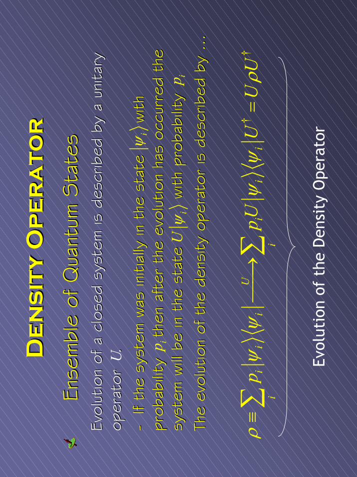
De
ns
ity
Op
er
at
or
De
ns
ity
Op
er
at
or
Ense
mbl
e of
Qua
ntum
Sta
tes
Ense
mbl
e of
Qua
ntum
Sta
tes
Evol
utio
n of
a c
lose
d sy
stem
is d
escr
ibed
by
a un
itary
Ev
olut
ion
of a
clo
sed
syst
em is
des
crib
ed b
y a
unita
ry
oper
ator
.
oper
ator
.
--If
the
syst
em w
as in
itial
ly in
the
sta
te
with
If
the
syst
em w
as in
itial
ly in
the
sta
te
with
pr
obab
ility
th
en a
fter
the
evo
lutio
n ha
s oc
curr
ed t
he
prob
ability
th
en a
fter
the
evo
lutio
n ha
s oc
curr
ed t
he
syst
em w
ill b
e in
the
sta
te
w
ith p
roba
bilit
ysy
stem
will b
e in
the
sta
te
w
ith p
roba
bilit
yTh
e ev
olut
ion
of t
he d
ensi
ty o
pera
tor
is d
escr
ibed
by
…Th
e ev
olut
ion
of t
he d
ensi
ty o
pera
tor
is d
escr
ibed
by
…
††
Ui
ii
ii
ii
ip
pUU
UU
ρψ
ψψ
ψρ
≡→
=∑
∑
iψ
ip
U
iUψ
Evol
utio
n of
the
Den
sity
Ope
rato
r
ip
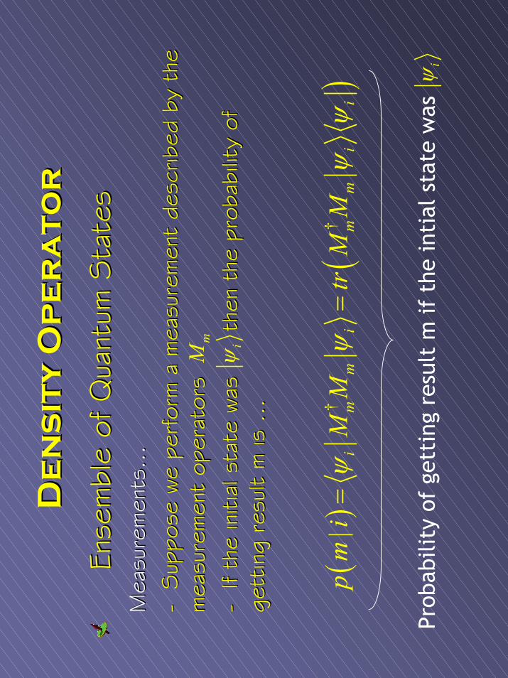
De
ns
ity
Op
er
at
or
De
ns
ity
Op
er
at
or
Ense
mbl
e of
Qua
ntum
Sta
tes
Ense
mbl
e of
Qua
ntum
Sta
tes
Mea
sure
men
ts…
Mea
sure
men
ts…
--Sup
pose
we
perfor
m a
mea
sure
men
t de
scrib
ed b
y th
e Sup
pose
we
perfor
m a
mea
sure
men
t de
scrib
ed b
y th
e m
easu
rem
ent
oper
ator
sm
easu
rem
ent
oper
ator
s--
If th
e in
itial
sta
te w
as
then
the
pro
babi
lity
of
If th
e in
itial
sta
te w
as
then
the
pro
babi
lity
of
gett
ing
resu
lt m
is …
gett
ing
resu
lt m
is …
()
()
††
|i
mm
im
mi
ipmi
MM
trMM
ψψ
ψψ
==
iψ
mM
Prob
abili
ty o
f ge
ttin
g re
sult
m if
the
inti
alst
ate
was
iψ
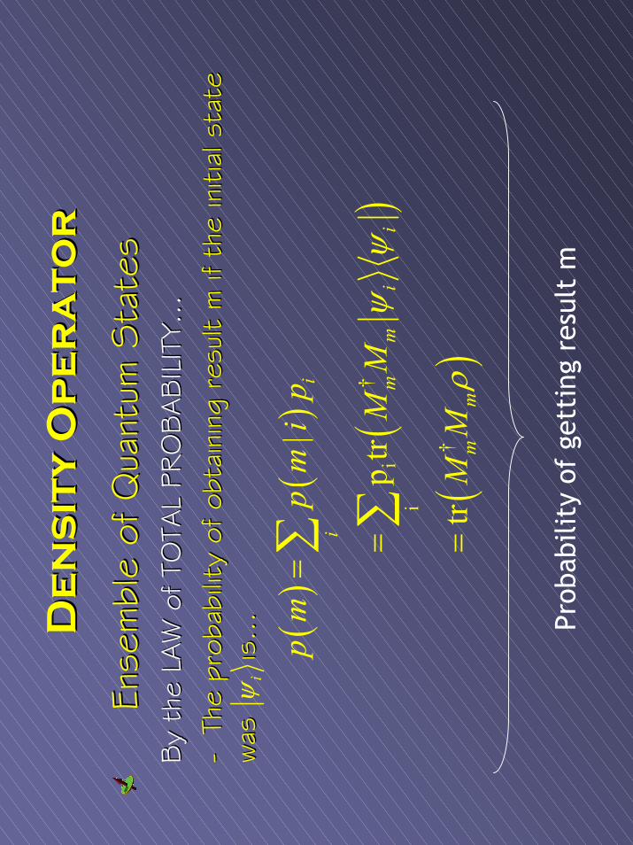
De
ns
ity
Op
er
at
or
De
ns
ity
Op
er
at
or
Ense
mbl
e of
Qua
ntum
Sta
tes
Ense
mbl
e of
Qua
ntum
Sta
tes
By
the
LAW
of TO
TAL
PRO
BABIL
ITY…
By
the
LAW
of TO
TAL
PRO
BABIL
ITY…
--Th
e pr
obab
ility
of ob
tain
ing
resu
lt m
if t
he in
itial
sta
te
The
prob
ability
of ob
tain
ing
resu
lt m
if t
he in
itial
sta
te
was
is
…was
is
… ()
() (
)
()
†i
i
†|
ptr
tr
ii
mm
ii
mm
pm
pmip MM
MM
ψψ
ρ
=
= =∑ ∑
Prob
abili
ty o
f ge
ttin
g re
sult
m
iψ
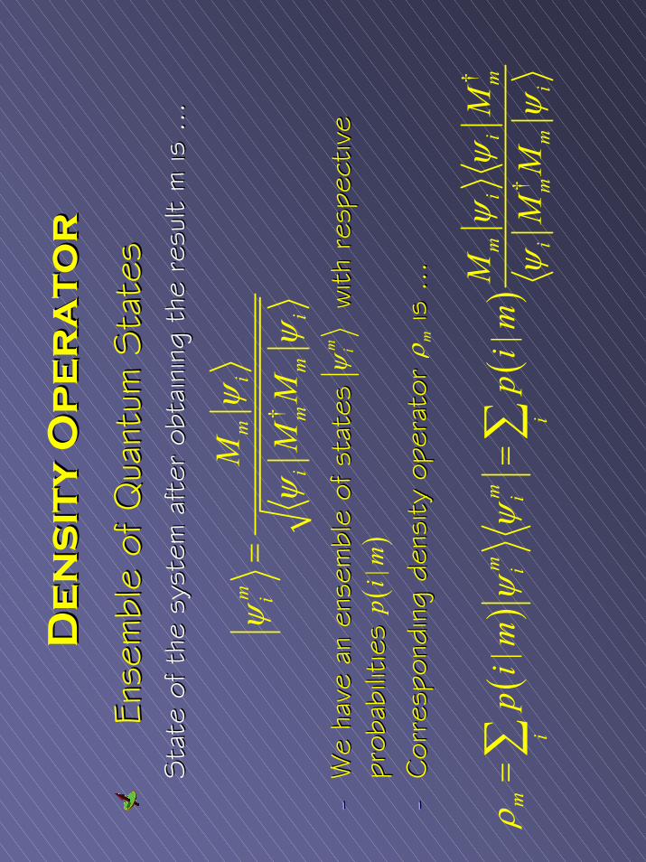
De
ns
ity
Op
er
at
or
De
ns
ity
Op
er
at
or
Ense
mbl
e of
Qua
ntum
Sta
tes
Ense
mbl
e of
Qua
ntum
Sta
tes
Sta
te o
f th
e sy
stem
aft
er o
btai
ning
the
res
ult
m is
…
Sta
te o
f th
e sy
stem
aft
er o
btai
ning
the
res
ult
m is
…
--W
e ha
ve a
n en
sem
ble
of s
tate
s
with
res
pect
ive
We
have
an
ense
mbl
e of
sta
tes
w
ith r
espe
ctive
prob
abilitie
s
prob
abilitie
s
--C
orre
spon
ding
den
sity
ope
rato
r
is
…C
orre
spon
ding
den
sity
ope
rato
r
is
…
†
mi
m i
im
mi
M MMψ
ψψ
ψ=
m iψ
()
|pim
mρ
()
()
†
†|
|m
ii
mm
mm
ii
ii
im
mi
MM
pim
pim
MM
ψψ
ρψ
ψψ
ψ=
=∑
∑
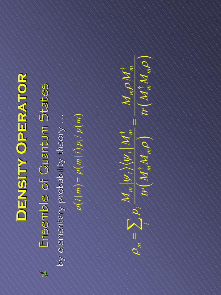
De
ns
ity
Op
er
at
or
De
ns
ity
Op
er
at
or
Ense
mbl
e of
Qua
ntum
Sta
tes
Ense
mbl
e of
Qua
ntum
Sta
tes
by e
lem
enta
ry p
roba
bilit
y th
eory
…
by e
lem
enta
ry p
roba
bilit
y th
eory
…
()
()
()
||
/i
pim
pmippm
= ()
()
††
††
mi
im
mm
mi
im
mm
m
MM
MM
ptrMM
trMM
ψψ
ρρ
ρρ
==
∑
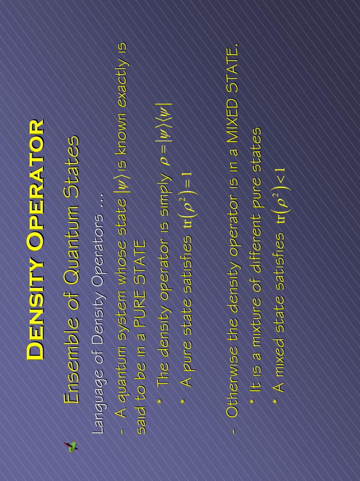
De
ns
ity
Op
er
at
or
De
ns
ity
Op
er
at
or
Ense
mbl
e of
Qua
ntum
Sta
tes
Ense
mbl
e of
Qua
ntum
Sta
tes
Lang
uage
of D
ensi
ty O
pera
tors
…
La
ngua
ge o
f D
ensi
ty O
pera
tors
…
--
A q
uant
um s
yste
m w
hose
sta
te
is
kno
wn
exac
tly is
A q
uant
um s
yste
m w
hose
sta
te
is
kno
wn
exac
tly is
sa
id t
o be
in a
PURE
STA
TEsa
id t
o be
in a
PURE
STA
TE*
The
den
sity
ope
rato
r is
sim
ply
* T
he d
ensi
ty o
pera
tor
is s
impl
y*
A p
ure
stat
e sa
tisfie
s *
A p
ure
stat
e sa
tisfie
s
--O
ther
wis
e th
e de
nsity
ope
rato
r is
in a
MIX
ED S
TATE
.O
ther
wis
e th
e de
nsity
ope
rato
r is
in a
MIX
ED S
TATE
.*
It is
a m
ixtu
re o
f di
ffere
nt p
ure
stat
es*
It is
a m
ixtu
re o
f di
ffere
nt p
ure
stat
es*
A m
ixed
sta
te s
atis
fies
* A m
ixed
sta
te s
atis
fies
()
2tr
1ρ
<
ρψ
ψ=
ψ
()
2tr
1ρ
=
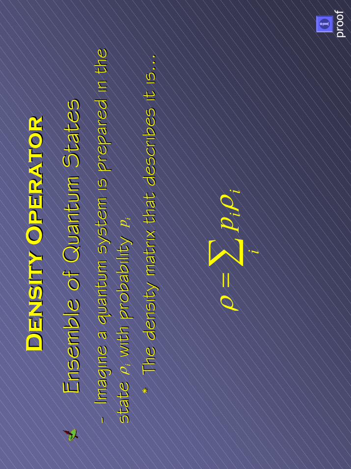
De
ns
ity
Op
er
at
or
De
ns
ity
Op
er
at
or
Ense
mbl
e of
Qua
ntum
Sta
tes
Ense
mbl
e of
Qua
ntum
Sta
tes
--Im
agin
e a
quan
tum
sys
tem
is p
repa
red
in t
he
Imag
ine
a qu
antu
m s
yste
m is
pre
pare
d in
the
st
ate
w
ith p
roba
bilit
y st
ate
w
ith p
roba
bilit
y *
The
den
sity
mat
rix t
hat
desc
ribes
it is
…*
The
den
sity
mat
rix t
hat
desc
ribes
it is
…
proo
f
ii
ip
ρρ
=∑
ipiρ
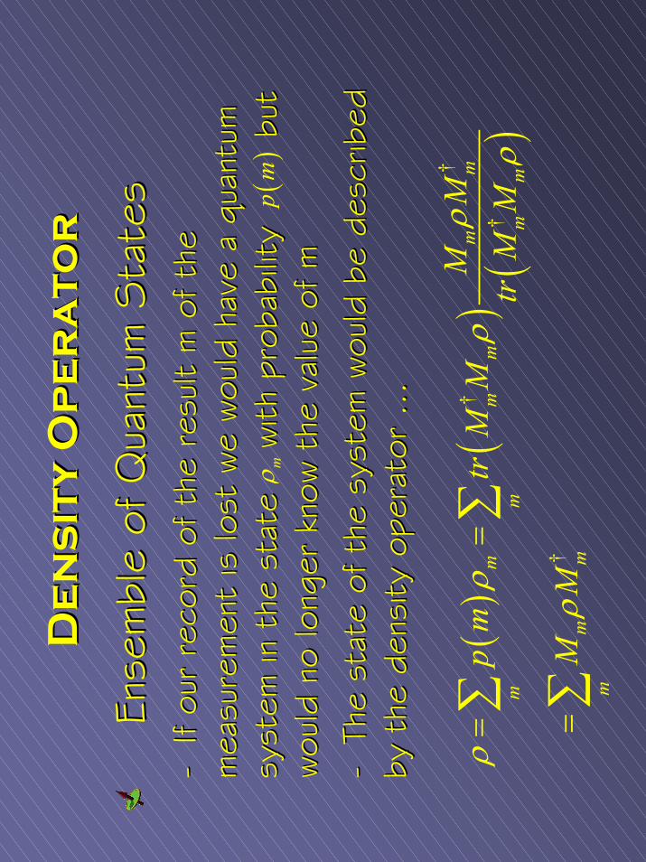
De
ns
ity
Op
er
at
or
De
ns
ity
Op
er
at
or
Ense
mbl
e of
Qua
ntum
Sta
tes
Ense
mbl
e of
Qua
ntum
Sta
tes
--If
our
reco
rd o
f th
e re
sult
m o
f th
e If
our
reco
rd o
f th
e re
sult
m o
f th
e m
easu
rem
ent
is lo
st w
e wou
ld h
ave
a qu
antu
m
mea
sure
men
t is
lost
we
wou
ld h
ave
a qu
antu
m
syst
em in
the
sta
te with
pro
babi
lity
b
ut
syst
em in
the
sta
te with
pro
babi
lity
b
ut
wou
ld n
o lo
nger
kno
w t
he v
alue
of m
wou
ld n
o lo
nger
kno
w t
he v
alue
of m
--Th
e st
ate
of t
he s
yste
m w
ould
be
desc
ribed
Th
e st
ate
of t
he s
yste
m w
ould
be
desc
ribed
by
the
den
sity
ope
rato
r …
by t
he d
ensi
ty o
pera
tor
…
()
()
()
††
†
†
mm
mm
mm
mm
m
mm
m
MM
pm
trMM
trMM
MM
ρρ
ρρ
ρ
ρ
==
=
∑∑
∑
mρ(
)pm
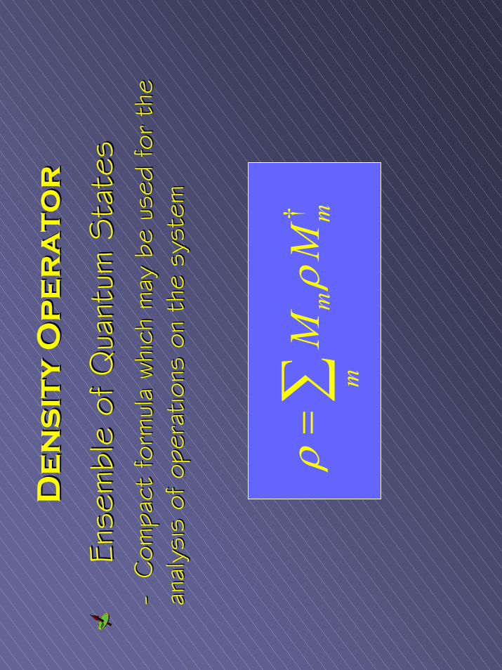
De
ns
ity
Op
er
at
or
De
ns
ity
Op
er
at
or
Ense
mbl
e of
Qua
ntum
Sta
tes
Ense
mbl
e of
Qua
ntum
Sta
tes
--Com
pact
for
mul
a whi
ch m
ay b
e us
ed for
the
Com
pact
for
mul
a whi
ch m
ay b
e us
ed for
the
an
alys
is o
f op
erat
ions
on
the
syst
eman
alys
is o
f op
erat
ions
on
the
syst
em †m
mmM
Mρ
ρ=∑
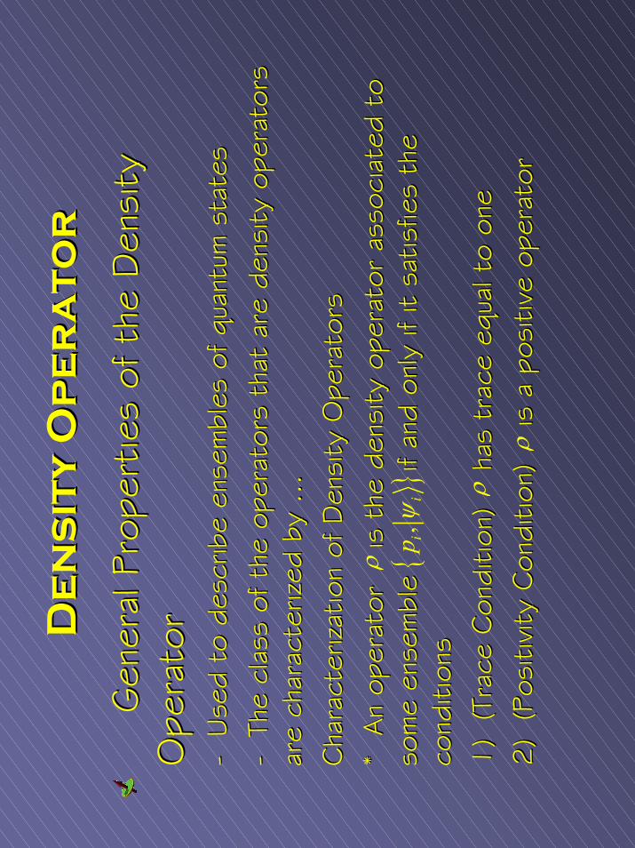
De
ns
ity
Op
er
at
or
De
ns
ity
Op
er
at
or
Gen
eral
Pro
pert
ies
of t
he D
ensi
ty
Gen
eral
Pro
pert
ies
of t
he D
ensi
ty
Ope
rato
rO
pera
tor
--Use
d to
des
crib
e en
sem
bles
of qu
antu
m s
tate
sUse
d to
des
crib
e en
sem
bles
of qu
antu
m s
tate
s--
The
clas
s of
the
ope
rato
rs t
hat
are
dens
ity o
pera
tors
Th
e cl
ass
of t
he o
pera
tors
tha
t ar
e de
nsity
ope
rato
rs
are
char
acte
rized
by
…ar
e ch
arac
teriz
ed b
y …
Cha
ract
erizat
ion
of D
ensi
ty O
pera
tors
Cha
ract
erizat
ion
of D
ensi
ty O
pera
tors
* A
n op
erat
or
is
the
den
sity
ope
rato
r as
soci
ated
to
* A
n op
erat
or
is
the
den
sity
ope
rato
r as
soci
ated
to
som
e en
sem
ble
if
and
only
if it
sat
isfie
s th
e so
me
ense
mbl
e
if
and
only
if it
sat
isfie
s th
e co
nditi
ons
cond
ition
s1
) (Tr
ace
Con
ditio
n) ha
s tr
ace
equa
l to
one
1) (Tr
ace
Con
ditio
n) ha
s tr
ace
equa
l to
one
2) (
2) (Po
sitiv
ityPo
sitiv
ityC
ondi
tion)
is a
pos
itive
ope
rato
rC
ondi
tion)
is a
pos
itive
ope
rato
r
ρ
, ii
pψ
ρ
ρ
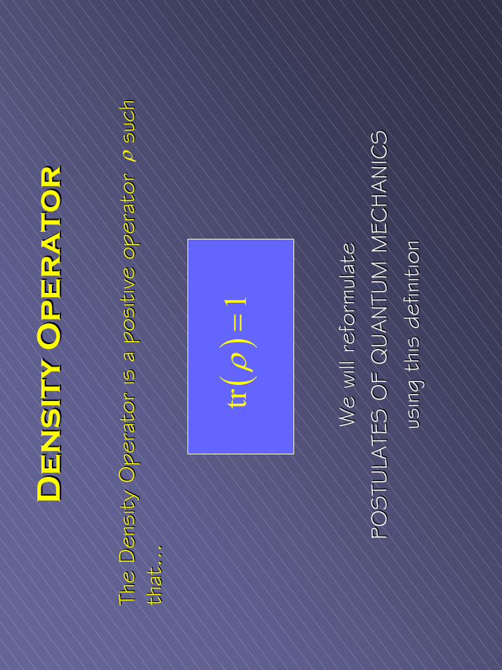
De
ns
ity
Op
er
at
or
De
ns
ity
Op
er
at
or
The
Den
sity
Ope
rato
r is
a p
ositi
ve o
pera
tor
s
uch
The
Den
sity
Ope
rato
r is
a p
ositi
ve o
pera
tor
s
uch
that
…th
at…
We
will r
efor
mul
ate
We
will r
efor
mul
ate
POSTU
LATE
S O
F Q
UANTU
M M
ECHANIC
S
POSTU
LATE
S O
F Q
UANTU
M M
ECHANIC
S
usin
g th
is d
efin
ition
usin
g th
is d
efin
ition
()
tr1
ρ=
ρ
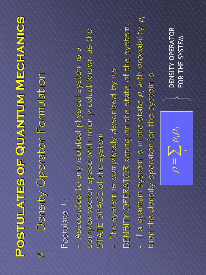
Po
st
ul
at
es
of
Qu
an
tu
m M
ec
ha
nic
sP
os
tu
la
te
s o
f Q
ua
nt
um
Me
ch
an
ics
Den
sity
Ope
rato
r Fo
rmul
atio
nD
ensi
ty O
pera
tor
Form
ulat
ion
Post
ulat
e 1
:Po
stul
ate
1:
--Ass
ocia
ted
to a
ny is
olat
ed p
hysi
cal s
yste
m is
a
Ass
ocia
ted
to a
ny is
olat
ed p
hysi
cal s
yste
m is
a
com
plex
vec
tor
spac
e with
inne
r pr
oduc
t kn
own
as t
he
com
plex
vec
tor
spac
e with
inne
r pr
oduc
t kn
own
as t
he
STA
TE S
PACE
of t
he s
yste
mSTA
TE S
PACE
of t
he s
yste
m--
The
syst
em is
com
plet
ely
desc
ribed
by
its
The
syst
em is
com
plet
ely
desc
ribed
by
its
DEN
SIT
Y O
PERATO
R a
ctin
g on
the
sta
te o
f th
e sy
stem
.D
ENSIT
Y O
PERATO
R a
ctin
g on
the
sta
te o
f th
e sy
stem
.--
If a
quan
tum
sys
tem
is in
the
sta
te
with
pro
babi
lity
If a
quan
tum
sys
tem
is in
the
sta
te
with
pro
babi
lity
then
the
den
sity
ope
rato
r fo
r th
e sy
stem
is …
then
the
den
sity
ope
rato
r fo
r th
e sy
stem
is …
ii
ip
ρρ
=∑
iρip
DEN
SITY
OPE
RATO
RFO
R TH
E SY
STEM
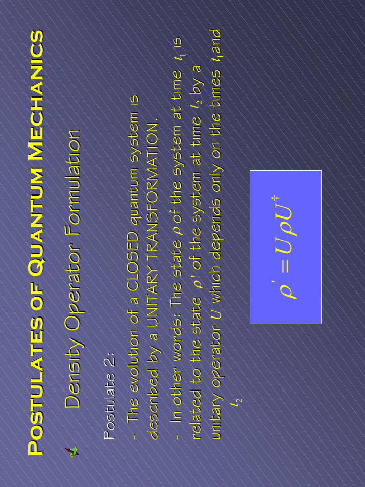
Po
st
ul
at
es
of
Qu
an
tu
m M
ec
ha
nic
sP
os
tu
la
te
s o
f Q
ua
nt
um
Me
ch
an
ics
Den
sity
Ope
rato
r Fo
rmul
atio
nD
ensi
ty O
pera
tor
Form
ulat
ion
Post
ulat
e 2
:Po
stul
ate
2:
--Th
e ev
olut
ion
of a
CLO
SED
qua
ntum
sys
tem
is
The
evol
utio
n of
a C
LOSED
qua
ntum
sys
tem
is
desc
ribed
by
a UNIT
ARY
TRANSFO
RM
ATI
ON.
desc
ribed
by
a UNIT
ARY
TRANSFO
RM
ATI
ON.
--In
oth
er w
ords
: Th
e st
ate
of
the
sys
tem
at
time
is
In
oth
er w
ords
: Th
e st
ate
of
the
sys
tem
at
time
is
re
late
d to
the
sta
te
o
f th
e sy
stem
at
time
b
y a
rela
ted
to t
he s
tate
of th
e sy
stem
at
time
b
y a
unita
ry o
pera
tor
w
hich
dep
ends
onl
y on
the
tim
es
and
un
itary
ope
rato
r
whi
ch d
epen
ds o
nly
on t
he t
imes
a
nd
'†
UU
ρρ
=
ρ'
ρ1t 1t
2t
2tU
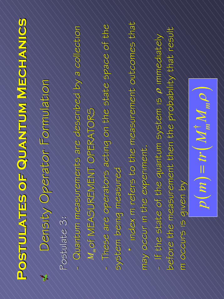
Po
st
ul
at
es
of
Qu
an
tu
m M
ec
ha
nic
sP
os
tu
la
te
s o
f Q
ua
nt
um
Me
ch
an
ics
Den
sity
Ope
rato
r Fo
rmul
atio
nD
ensi
ty O
pera
tor
Form
ulat
ion
Post
ulat
e 3
:Po
stul
ate
3:
--Q
uant
um m
easu
rem
ents
are
des
crib
ed b
y a
colle
ctio
nQ
uant
um m
easu
rem
ents
are
des
crib
ed b
y a
colle
ctio
nof
MEA
SUREM
ENT
OPE
RATO
RS
of M
EASUREM
ENT
OPE
RATO
RS
--Th
ese
are
oper
ator
s ac
ting
on t
he s
tate
spa
ce o
f th
e Th
ese
are
oper
ator
s ac
ting
on t
he s
tate
spa
ce o
f th
e sy
stem
bei
ng m
easu
red
syst
em b
eing
mea
sure
d*
inde
x m
ref
ers
to t
he m
easu
rem
ent
outc
omes
tha
t *
inde
x m
ref
ers
to t
he m
easu
rem
ent
outc
omes
tha
t m
ay o
ccur
in t
he e
xper
imen
t.m
ay o
ccur
in t
he e
xper
imen
t.--
If th
e st
ate
of t
he q
uant
um s
yste
m is
imm
edia
tely
If
the
stat
e of
the
qua
ntum
sys
tem
is
im
med
iate
ly
befo
re t
he m
easu
rem
ent
then
the
pro
babi
lity
that
res
ult
befo
re t
he m
easu
rem
ent
then
the
pro
babi
lity
that
res
ult
m o
ccur
s is
given
by
m o
ccur
s is
given
by
()
()
† mm
pm
trMM
ρ=
mM
ρ
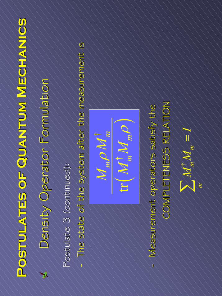
Po
st
ul
at
es
of
Qu
an
tu
m M
ec
ha
nic
sP
os
tu
la
te
s o
f Q
ua
nt
um
Me
ch
an
ics
()
†
†tr
mm
mm
MM
MMρ
ρ
Den
sity
Ope
rato
r Fo
rmul
atio
nD
ensi
ty O
pera
tor
Form
ulat
ion
Post
ulat
e 3
(co
ntin
ued)
:Po
stul
ate
3 (co
ntin
ued)
:--
The
stat
e of
the
sys
tem
aft
er t
he m
easu
rem
ent
isTh
e st
ate
of t
he s
yste
m a
fter
the
mea
sure
men
t is
--M
easu
rem
ent
oper
ator
s sa
tisfy
the
M
easu
rem
ent
oper
ator
s sa
tisfy
the
CO
MPL
ETEN
ESS R
ELATI
ON
CO
MPL
ETEN
ESS R
ELATI
ON
† mm
mMM
I=
∑
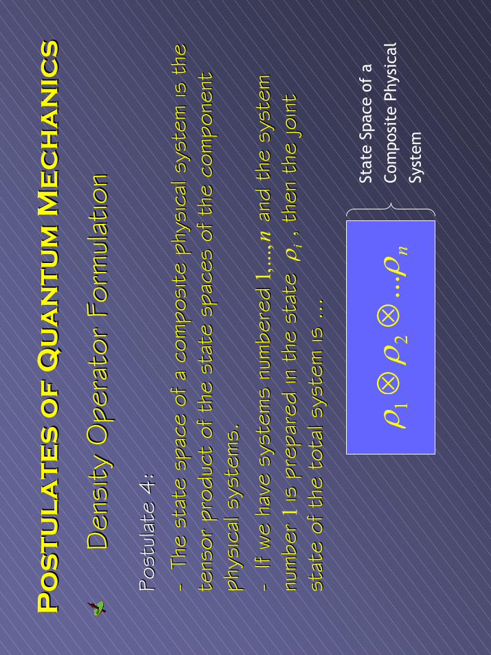
Po
st
ul
at
es
of
Qu
an
tu
m M
ec
ha
nic
sP
os
tu
la
te
s o
f Q
ua
nt
um
Me
ch
an
ics
Den
sity
Ope
rato
r Fo
rmul
atio
nD
ensi
ty O
pera
tor
Form
ulat
ion
Post
ulat
e 4
:
Post
ulat
e 4
:
--Th
e st
ate
spac
e of
a c
ompo
site
phy
sica
l sys
tem
is t
he
The
stat
e sp
ace
of a
com
posi
te p
hysi
cal s
yste
m is
the
te
nsor
pro
duct
of th
e st
ate
spac
es o
f th
e co
mpo
nent
te
nsor
pro
duct
of th
e st
ate
spac
es o
f th
e co
mpo
nent
ph
ysic
al s
yste
ms.
phys
ical
sys
tem
s.--
If we
have
sys
tem
s nu
mbe
red
and
the
syst
em
If we
have
sys
tem
s nu
mbe
red
and
the
syst
em
num
ber
is
pre
pare
d in
the
sta
te
,
the
n th
e jo
int
num
ber
is
pre
pare
d in
the
sta
te
,
the
n th
e jo
int
stat
e of
the
tot
al s
yste
m is
…st
ate
of t
he t
otal
sys
tem
is …
12
...n
ρρ
ρ⊗
⊗
iρ1,
...,n
1
Stat
e Sp
ace
of a
Com
posi
te P
hysi
cal
Syst
em
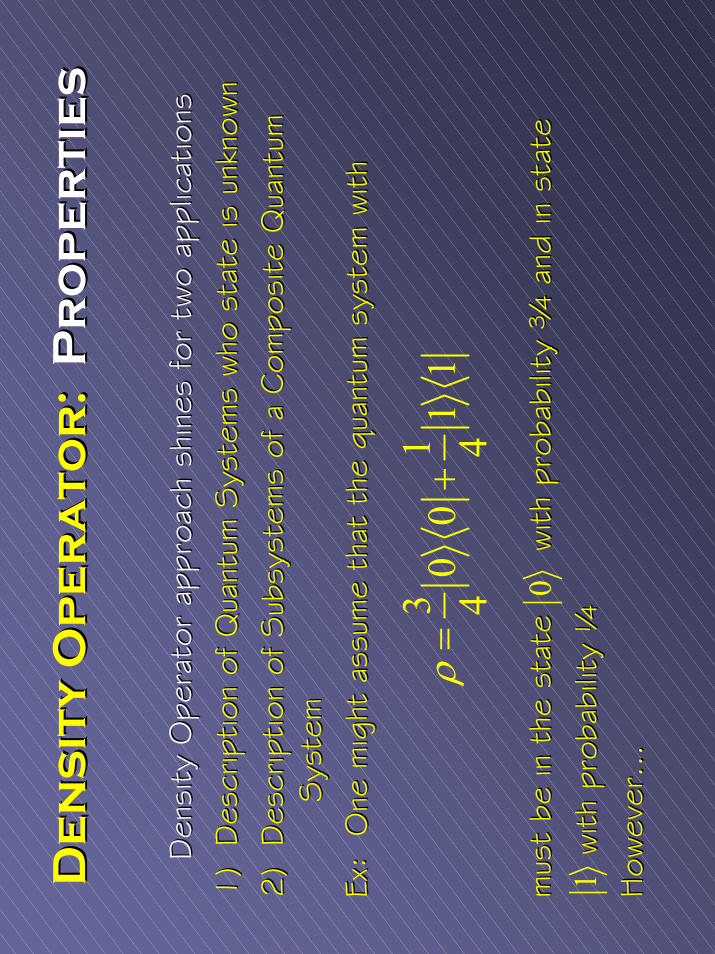
De
ns
ity
Op
er
at
or
: D
en
sit
y O
pe
ra
to
r:
Pr
op
er
tie
sP
ro
pe
rt
ies
Den
sity
Ope
rato
r ap
proa
ch s
hine
s fo
r tw
o ap
plic
atio
nsD
ensi
ty O
pera
tor
appr
oach
shi
nes
for
two
appl
icat
ions
1) D
escr
iptio
n of
Qua
ntum
Sys
tem
s who
sta
te is
unk
nown
1) D
escr
iptio
n of
Qua
ntum
Sys
tem
s who
sta
te is
unk
nown
2) D
escr
iptio
n of
Sub
syst
ems
of a
Com
posi
te Q
uant
um
2
) D
escr
iptio
n of
Sub
syst
ems
of a
Com
posi
te Q
uant
um
Sys
tem
Sys
tem
Ex:
One
mig
ht a
ssum
e th
at t
he q
uant
um s
yste
m w
ithEx
: O
ne m
ight
ass
ume
that
the
qua
ntum
sys
tem
with
mus
t be
in t
he s
tate
with
pro
babi
lity
¾ a
nd in
sta
tem
ust
be in
the
sta
te
with
pro
babi
lity
¾ a
nd in
sta
tewith
pro
babi
lity
¼with
pro
babi
lity
¼How
ever
…How
ever
…
31
00
11
44
ρ=
+
01
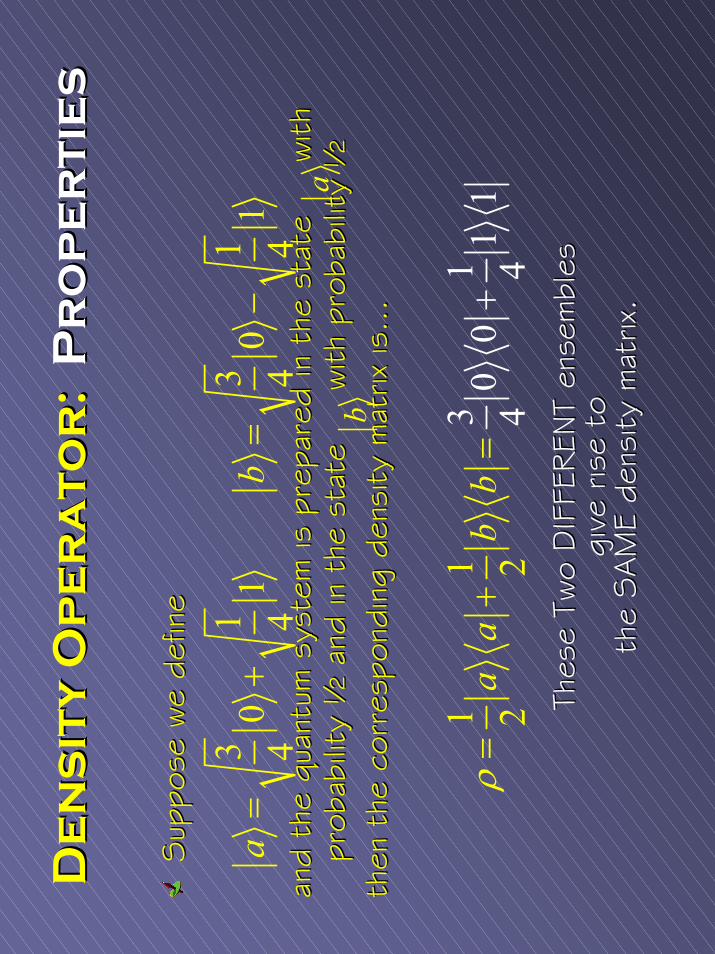
De
ns
ity
Op
er
at
or
: D
en
sit
y O
pe
ra
to
r:
Pr
op
er
tie
sP
ro
pe
rt
ies
Sup
pose
we
defin
eSup
pose
we
defin
e
and
the
quan
tum
sys
tem
is p
repa
red
in t
he s
tate
with
an
d th
e qu
antu
m s
yste
m is
pre
pare
d in
the
sta
te
w
ith
prob
ability
½ a
nd in
the
sta
te
w
ith p
roba
bilit
y ½
prob
ability
½ a
nd in
the
sta
te
w
ith p
roba
bilit
y ½
then
the
cor
resp
ondi
ng d
ensi
ty m
atrix
is…
then
the
cor
resp
ondi
ng d
ensi
ty m
atrix
is…
Thes
e Tw
o D
IFFE
REN
T en
sem
bles
Th
ese
Two
DIF
FEREN
T en
sem
bles
gi
ve r
ise
to
give
ris
e to
th
e SAM
E de
nsity
mat
rix.
the
SAM
E de
nsity
mat
rix.
31
31
01
0
14
44
4a
b=
+=
−
11
22
31
00
11
44
aa
bb
ρ+
=+
=
ab
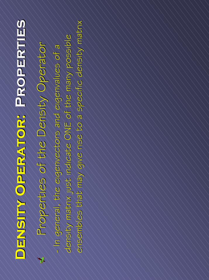
De
ns
ity
Op
er
at
or
: D
en
sit
y O
pe
ra
to
r:
Pr
op
er
tie
sP
ro
pe
rt
ies
Prop
ertie
s of
the
Den
sity
Ope
rato
rPr
oper
ties
of t
he D
ensi
ty O
pera
tor
--In
gen
eral
, th
e ei
genv
ecto
rs a
nd
In g
ener
al,
the
eige
nvec
tors
and
eig
enva
lues
eige
nval
ues
of a
of
a
dens
ity m
atrix
just
indi
cate
ONE
of t
he m
any
poss
ible
de
nsity
mat
rix ju
st in
dica
te O
NE
of t
he m
any
poss
ible
en
sem
bles
tha
t m
ay g
ive
rise
to a
spe
cific
den
sity
mat
rixen
sem
bles
tha
t m
ay g
ive
rise
to a
spe
cific
den
sity
mat
rix
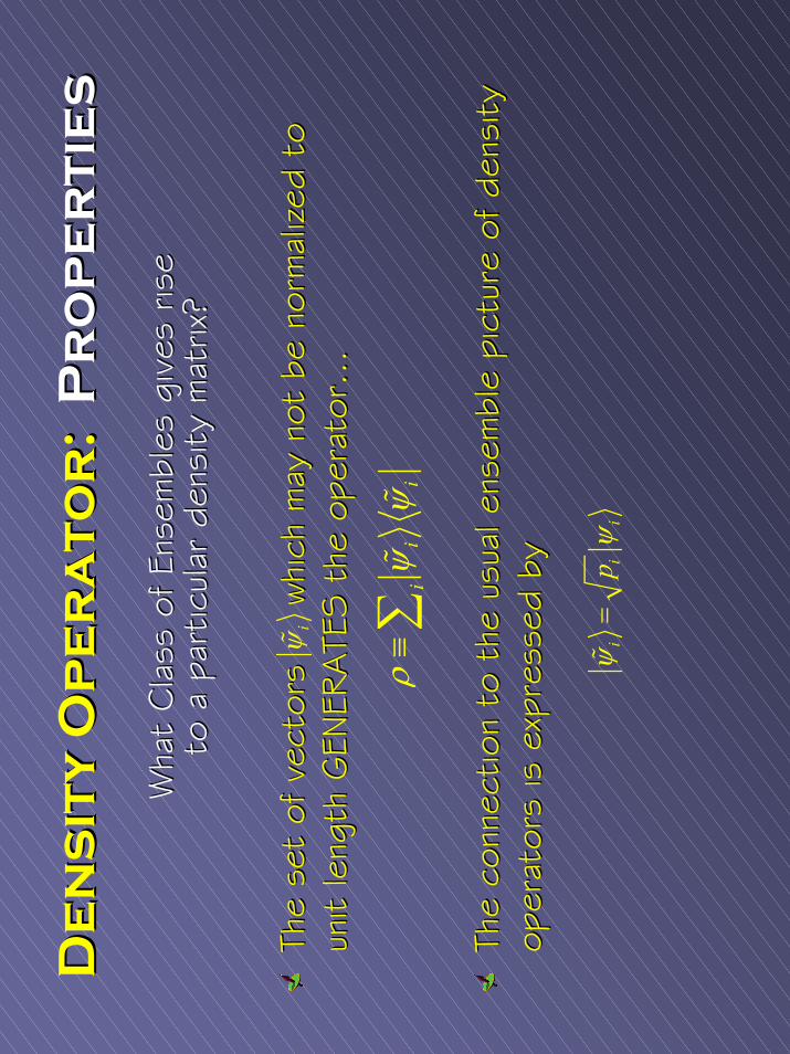
De
ns
ity
Op
er
at
or
: D
en
sit
y O
pe
ra
to
r:
Pr
op
er
tie
sP
ro
pe
rt
ies
Wha
t C
lass
of En
sem
bles
gives
ris
e W
hat
Cla
ss o
f En
sem
bles
gives
ris
e to
a p
artic
ular
den
sity
mat
rix?
to a
par
ticul
ar d
ensi
ty m
atrix
?
The
set
of v
ecto
rs
w
hich
may
not
be
norm
alized
to
The
set
of v
ecto
rs
w
hich
may
not
be
norm
alized
to
unit
leng
th G
ENER
ATE
S t
he o
pera
tor…
unit
leng
th G
ENER
ATE
S t
he o
pera
tor…
The
conn
ectio
n to
the
usu
al e
nsem
ble
pict
ure
of d
ensi
ty
The
conn
ectio
n to
the
usu
al e
nsem
ble
pict
ure
of d
ensi
ty
oper
ator
s is
exp
ress
ed b
yop
erat
ors
is e
xpre
ssed
by
iψ% i
ii
pψ
ψ=
%
ii
iρ
ψψ
≡∑
%%
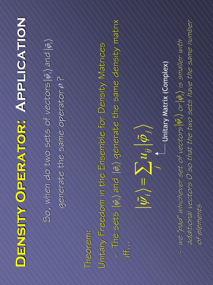
De
ns
ity
Op
er
at
or
: D
en
sit
y O
pe
ra
to
r:
Ap
pl
ica
tio
nA
pp
lic
at
ion
So,
whe
n do
two
sets
of ve
ctor
s
an
d
So,
whe
n do
two
sets
of ve
ctor
s
an
d
ge
nera
te t
he s
ame
oper
ator
?
gene
rate
the
sam
e op
erat
or
?
Theo
rem
:
Theo
rem
:
Uni
tary
Fre
edom
in t
he E
nsem
ble
for
Den
sity
Mat
rices
Uni
tary
Fre
edom
in t
he E
nsem
ble
for
Den
sity
Mat
rices
--Th
e se
ts
and
gen
erat
e th
e sa
me
dens
ity m
atrix
Th
e se
ts
and
gen
erat
e th
e sa
me
dens
ity m
atrix
iffiff
…… --we
"pad
" whi
chev
er s
et o
f vec
tors
or
is
sm
alle
r with
we
"pad
" whi
chev
er s
et o
f vec
tors
or
is
sm
alle
r with
addi
tiona
l vec
tors
0 s
o th
at t
he t
wo
sets
hav
e th
e sa
me
num
ber
addi
tiona
l vec
tors
0 s
o th
at t
he t
wo
sets
hav
e th
e sa
me
num
ber
of e
lem
ents
of e
lem
ents
iψ%
iij
jju
ψϕ
=∑
%%
iϕ%ρ
iψ%
iϕ%
iϕ%
Uni
tary
Mat
rix
(Com
plex
)
iψ%
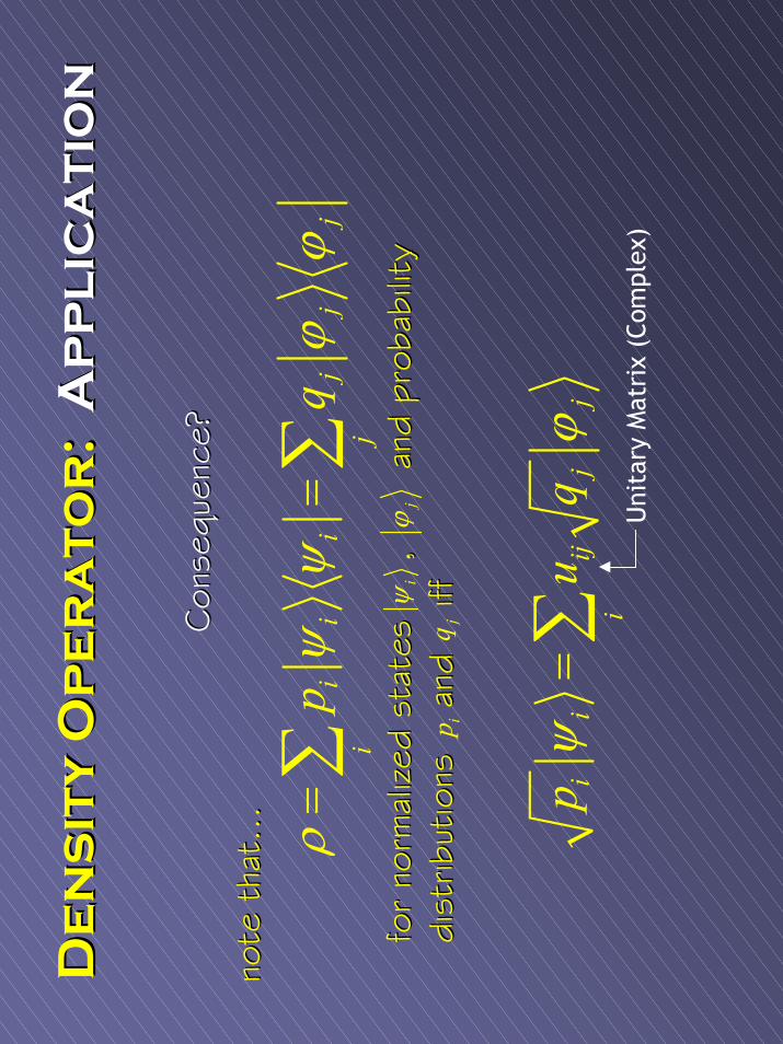
De
ns
ity
Op
er
at
or
: D
en
sit
y O
pe
ra
to
r:
Ap
pl
ica
tio
nA
pp
lic
at
ion
Con
sequ
ence
?Con
sequ
ence
?no
te t
hat…
note
tha
t…
for
norm
alized
sta
tes
,
and
prob
ability
fo
r no
rmal
ized
sta
tes
,
and
prob
ability
di
strib
utio
ns
an
d
di
strib
utio
ns
an
d
iffiffi
ψ
ii
ij
jj
ij
pq
ρψ
ψϕ
ϕ=
=∑
∑j
ϕ
ipjq
ii
ijj
ji
pu
qψ
ϕ=∑
Uni
tary
Mat
rix
(Com
plex
)
Re
du
ce
d D
en
sit
y O
pe
ra
to
rR
ed
uc
ed
De
ns
ity
Op
er
at
or
The
Red
uced
Den
sity
Ope
rato
r is
a d
escr
iptiv
e to
ol for
SUBSYS
TEM
S o
f a
com
posi
te q
uant
um s
yste
m
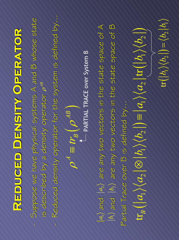
Re
du
ce
d D
en
sit
y O
pe
ra
to
rR
ed
uc
ed
De
ns
ity
Op
er
at
or
--Sup
pose
we
have
phy
sica
l sys
tem
s A a
nd B
who
se s
tate
Sup
pose
we
have
phy
sica
l sys
tem
s A a
nd B
who
se s
tate
is
des
crib
ed b
y a
dens
ity o
pera
tor
is d
escr
ibed
by
a de
nsity
ope
rato
r--
Red
uced
den
sity
ope
rato
r fo
r th
e sy
stem
is d
efin
ed b
y…Red
uced
den
sity
ope
rato
r fo
r th
e sy
stem
is d
efin
ed b
y…
and
ar
e an
y tw
o ve
ctor
s in
the
sta
te s
pace
of A
and
ar
e an
y tw
o ve
ctor
s in
the
sta
te s
pace
of A
and
ar
e an
y tw
o ve
ctor
s in
the
sta
te s
pace
of B
and
ar
e an
y tw
o ve
ctor
s in
the
sta
te s
pace
of B
Part
ial T
race
ove
r B is
def
ined
by…
Part
ial T
race
ove
r B is
def
ined
by…
ABρ
()
AAB
Btrρ
ρ≡
PART
IAL
TRAC
E ov
er S
yste
m B
()
()
12
12
12
12
trtr
Ba
abb
aa
bb
⊗≡
1a2a
1b2b
()
12
21
trbb
bb
=
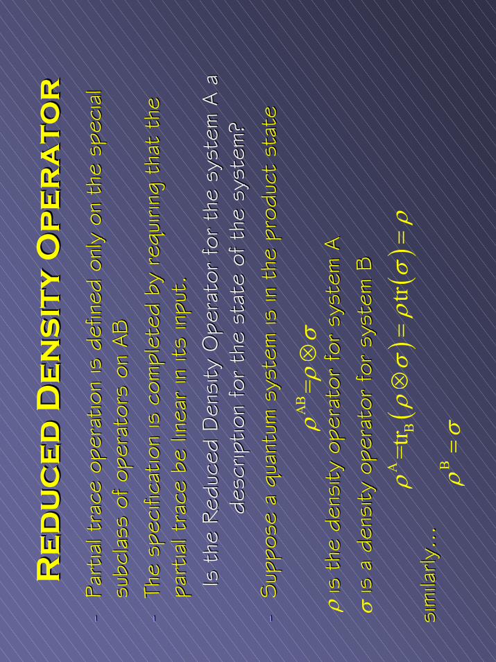
Re
du
ce
d D
en
sit
y O
pe
ra
to
rR
ed
uc
ed
De
ns
ity
Op
er
at
or
--Pa
rtia
l tra
ce o
pera
tion
is d
efin
ed o
nly
on t
he s
peci
al
Part
ial t
race
ope
ratio
n is
def
ined
onl
y on
the
spe
cial
su
bcla
ss o
f op
erat
ors
on A
Bsu
bcla
ss o
f op
erat
ors
on A
B--
The
spec
ifica
tion
is c
ompl
eted
by
requ
iring
tha
t th
e Th
e sp
ecifi
catio
n is
com
plet
ed b
y re
quiri
ng t
hat
the
part
ial t
race
be
linea
r in
its
inpu
t.pa
rtia
l tra
ce b
e lin
ear
in it
s in
put.
Is t
he R
educ
ed D
ensi
ty O
pera
tor
for
the
syst
em A
a
Is t
he R
educ
ed D
ensi
ty O
pera
tor
for
the
syst
em A
a
desc
riptio
n fo
r th
e st
ate
of t
he s
yste
m?
desc
riptio
n fo
r th
e st
ate
of t
he s
yste
m?
--Sup
pose
a q
uant
um s
yste
m is
in t
he p
rodu
ct s
tate
Sup
pose
a q
uant
um s
yste
m is
in t
he p
rodu
ct s
tate
is t
he d
ensi
ty o
pera
tor
for
syst
em A
is t
he d
ensi
ty o
pera
tor
for
syst
em A
is a
den
sity
ope
rato
r fo
r sy
stem
Bis
a d
ensi
ty o
pera
tor
for
syst
em B
sim
ilarly
…si
mila
rly…
()
()
AB
=tr
trρ
ρσ
ρσ
ρ⊗
==
AB
=ρ
ρσ
⊗
Bρ
σ=
ρ σ
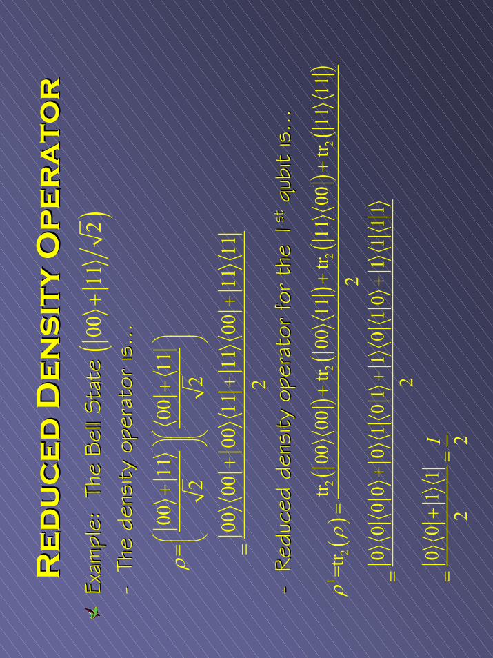
Re
du
ce
d D
en
sit
y O
pe
ra
to
rR
ed
uc
ed
De
ns
ity
Op
er
at
or
Exam
ple:
Th
e Bel
l Sta
te
Exam
ple:
Th
e Bel
l Sta
te
--Th
e de
nsity
ope
rato
r is
…Th
e de
nsity
ope
rato
r is
…
--Red
uced
den
sity
ope
rato
r fo
r th
e 1
Red
uced
den
sity
ope
rato
r fo
r th
e 1
ststqu
bit
qubi
tis
…is
…
0011
0011
=2
200
0000
1111
0011
11
2
ρ
+
+
++
+=
()
0011
2+
()
()
()
()
()
22
22
12
tr00
00tr
0011
tr11
00tr
1111
=tr
20
00
00
10
11
01
01
11
1
20
01
1
I
ρρ
++
+=
++
+=
+=
=2
2
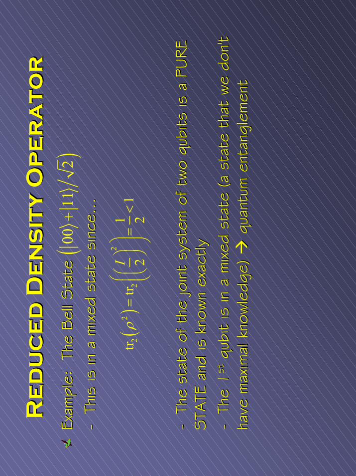
Re
du
ce
d D
en
sit
y O
pe
ra
to
rR
ed
uc
ed
De
ns
ity
Op
er
at
or
Exam
ple:
Th
e Bel
l Sta
te
Exam
ple:
Th
e Bel
l Sta
te
--Th
is is
in a
mixed
sta
te s
ince
…Th
is is
in a
mixed
sta
te s
ince
…
--Th
e st
ate
of t
he jo
int
syst
em o
f tw
o Th
e st
ate
of t
he jo
int
syst
em o
f tw
o qu
bits
qubi
tsis
a P
URE
is a
PURE
STA
TE a
nd is
kno
wn
exac
tlySTA
TE a
nd is
kno
wn
exac
tly--
The
1Th
e 1
ststqu
bit
qubi
tis
in a
mixed
sta
te (a
stat
e th
at w
e do
n't
is in
a m
ixed
sta
te (a
stat
e th
at w
e do
n't
have
max
imal
kno
wle
dge)
ha
ve m
axim
al k
nowle
dge)
qu
antu
m e
ntan
glem
ent
quan
tum
ent
angl
emen
t
()
0011
2+
()
22
22
1tr
tr1
22
Iρ
==
<
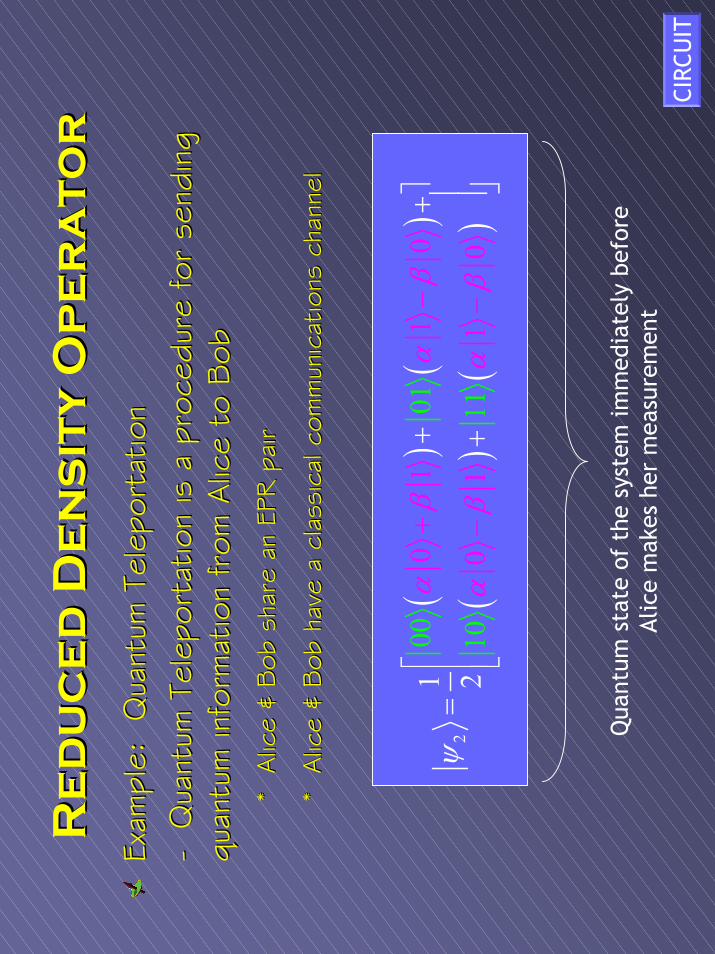
Re
du
ce
d D
en
sit
y O
pe
ra
to
rR
ed
uc
ed
De
ns
ity
Op
er
at
or
Exam
ple:
Q
uant
um T
elep
orta
tion
Exam
ple:
Q
uant
um T
elep
orta
tion
--Q
uant
um T
elep
orta
tion
is a
pro
cedu
re for
sen
ding
Q
uant
um T
elep
orta
tion
is a
pro
cedu
re for
sen
ding
qu
antu
m in
form
atio
n from
Alic
e to
Bob
quan
tum
info
rmat
ion
from
Alic
e to
Bob
* A
lice
& Bob
sha
re a
n EP
R p
air
* A
lice
& Bob
sha
re a
n EP
R p
air
* A
lice
& Bob
hav
e a
clas
sica
l com
mun
icat
ions
cha
nnel
* A
lice
& Bob
hav
e a
clas
sica
l com
mun
icat
ions
cha
nnel
()
()
()
()
2
0001
101
01
10
02
10
11
1
αβ
αβ
αψ
βα
β
+−
−
++
=+
−
Qua
ntum
sta
te o
f th
e sy
stem
imm
edia
tely
bef
ore
Alic
e m
akes
her
mea
sure
men
tCI
RCU
IT
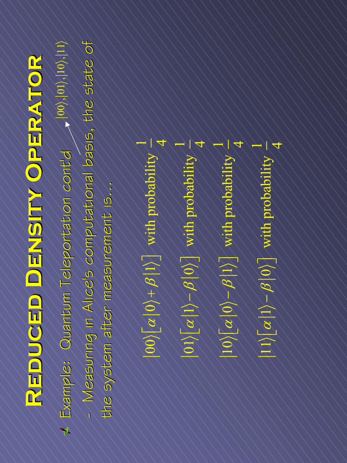
Re
du
ce
d D
en
sit
y O
pe
ra
to
rR
ed
uc
ed
De
ns
ity
Op
er
at
or
Exam
ple:
Q
uant
um T
elep
orta
tion
cont
'd
Exam
ple:
Q
uant
um T
elep
orta
tion
cont
'd
--M
easu
ring
in A
lice'
s co
mpu
tatio
nal b
asis
, th
e st
ate
of
Mea
surin
g in
Alic
e's
com
puta
tiona
l bas
is,
the
stat
e of
th
e sy
stem
aft
er m
easu
rem
ent
is…
the
syst
em a
fter
mea
sure
men
t is
…
00,0
1,1
0,1
1
100
01
with
pro
babi
lity
4 101
10
with
pro
babi
lity
4 110
01
with
pro
babi
lity
4 111
10
with
pro
babi
lity
4
αβ
αβ
αβ
αβ
+
−
−
−
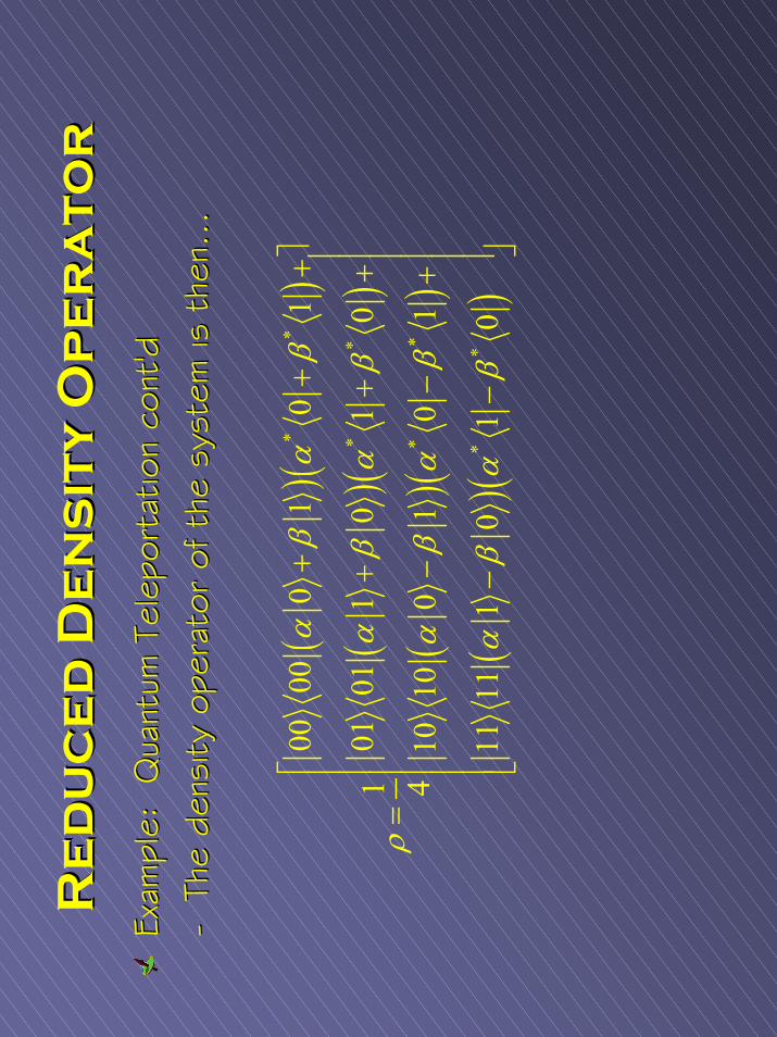
Re
du
ce
d D
en
sit
y O
pe
ra
to
rR
ed
uc
ed
De
ns
ity
Op
er
at
or
Exam
ple:
Q
uant
um T
elep
orta
tion
cont
'd
Exam
ple:
Q
uant
um T
elep
orta
tion
cont
'd
--Th
e de
nsity
ope
rato
r of
the
sys
tem
is t
hen…
The
dens
ity o
pera
tor
of t
he s
yste
m is
the
n…
() (
)(
) ()
() (
)(
) ()
**
**
**
**
0000
01
01
0101
10
10
1 410
100
10
1
1111
10
10
αβ
αβ
αβ
αβ
ρα
βα
β
αβ
αβ
++
+
+
++
=
−
−+
−−
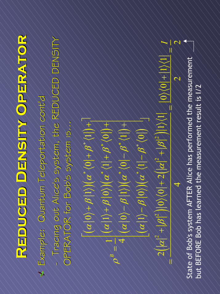
Re
du
ce
d D
en
sit
y O
pe
ra
to
rR
ed
uc
ed
De
ns
ity
Op
er
at
or
() (
)(
) ()
() (
)(
) ()
()
()
**
**
**
**
22
22
01
01
10
10
1 40
10
1
10
10
20
02
11
00
11
42
2
B
I
αβ
αβ
αβ
αβ
ρα
βα
β
αβ
αβ
αβ
αβ
++
+
+
++
=
−
−+
−−
++
++
==
=
Exam
ple:
Q
uant
um T
elep
orta
tion
cont
'd
Exam
ple:
Q
uant
um T
elep
orta
tion
cont
'd
--Tr
acin
g ou
t Alic
e's
syst
em, th
e RED
UC
ED D
ENSIT
Y Tr
acin
g ou
t Alic
e's
syst
em, th
e RED
UC
ED D
ENSIT
Y O
PERATO
R for
Bob
's s
yste
m is
…O
PERATO
R for
Bob
's s
yste
m is
…
Stat
e of
Bob
's sy
stem
AFT
ER A
lice
has
perf
orm
ed t
he m
easu
rem
ent
but
BEFO
RE B
ob h
as le
arne
d th
e m
easu
rem
ent
resu
lt is
I/2
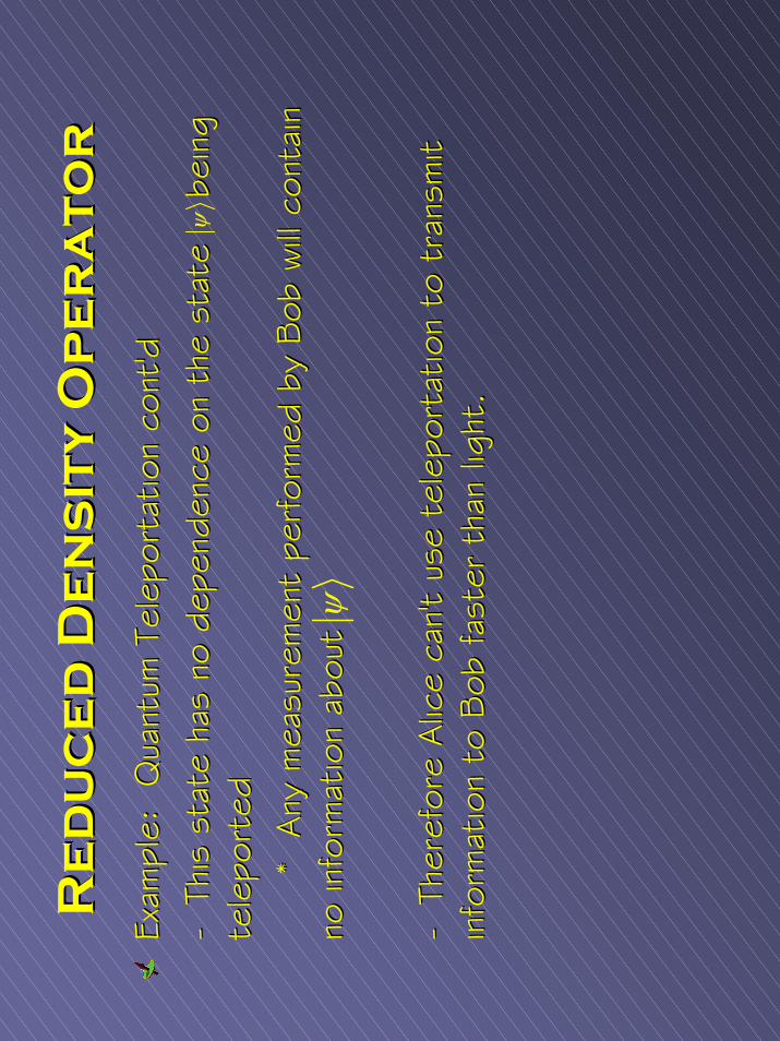
Re
du
ce
d D
en
sit
y O
pe
ra
to
rR
ed
uc
ed
De
ns
ity
Op
er
at
or
Exam
ple:
Q
uant
um T
elep
orta
tion
cont
'dEx
ampl
e:
Qua
ntum
Tel
epor
tatio
n co
nt'd
--Th
is s
tate
has
no
depe
nden
ce o
n th
e st
ate
b
eing
Th
is s
tate
has
no
depe
nden
ce o
n th
e st
ate
b
eing
te
lepo
rted
tele
port
ed*
Any
mea
sure
men
t pe
rfor
med
by
Bob
will c
onta
in
* A
ny m
easu
rem
ent
perfor
med
by
Bob
will c
onta
in
no in
form
atio
n ab
out
no in
form
atio
n ab
out
--Th
eref
ore
Alic
e ca
n't
use
tele
port
atio
n to
tra
nsm
it Th
eref
ore
Alic
e ca
n't
use
tele
port
atio
n to
tra
nsm
it in
form
atio
n to
Bob
fas
ter
than
ligh
t.in
form
atio
n to
Bob
fas
ter
than
ligh
t.
ψ
ψ
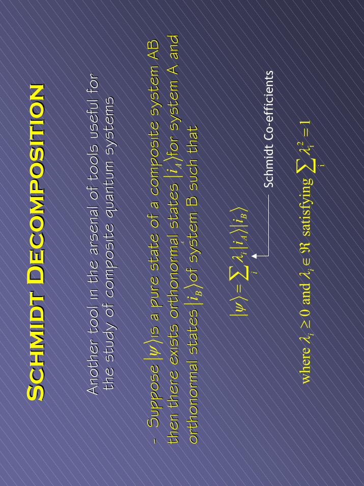
Sc
hm
idt
De
co
mp
os
itio
nS
ch
mid
t D
ec
om
po
sit
ion
Ano
ther
too
l in
the
arse
nal o
f to
ols
usef
ul for
Ano
ther
too
l in
the
arse
nal o
f to
ols
usef
ul for
th
e st
udy
of c
ompo
site
qua
ntum
sys
tem
sth
e st
udy
of c
ompo
site
qua
ntum
sys
tem
s
--Sup
pose
is a
pur
e st
ate
of a
com
posi
te s
yste
m A
B
Sup
pose
is a
pur
e st
ate
of a
com
posi
te s
yste
m A
B
then
the
re e
xists
th
en t
here
exis
ts o
rtho
norm
alor
thon
orm
alst
ates
for
sys
tem
A a
nd
stat
es
for
sys
tem
A a
nd
orth
onor
mal
orth
onor
mal
stat
es
o
f sy
stem
B s
uch
that
stat
es
o
f sy
stem
B s
uch
that
ψAi
iA
Bi
ii
ψλ
=∑
2 ii
whe
re
0 an
d sa
tisfy
ing
1i
iλ
λλ
≥∈ℜ
=∑
Schm
idt
Co-e
ffic
ient
s
A
Bi
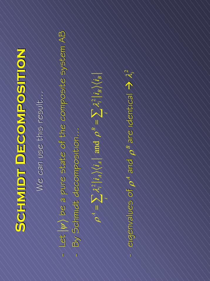
Sc
hm
idt
De
co
mp
os
itio
nS
ch
mid
t D
ec
om
po
sit
ion
We
can
use
this
res
ult…
We
can
use
this
res
ult…
--Le
t
b
e a
pure
sta
te o
f th
e co
mpo
site
sys
tem
AB
Let
be
a pu
re s
tate
of th
e co
mpo
site
sys
tem
AB
--By
Sch
mid
t de
com
posi
tion…
By
Sch
mid
t de
com
posi
tion…
--ei
genv
alue
sei
genv
alue
sof
and
are
iden
tical
of
and
are
iden
tical
ψ
22
and
A
Bi
AA
iB
Bi
iii
ii
ρλ
ρλ
==
∑∑
Aρ
Bρ
2 iλ
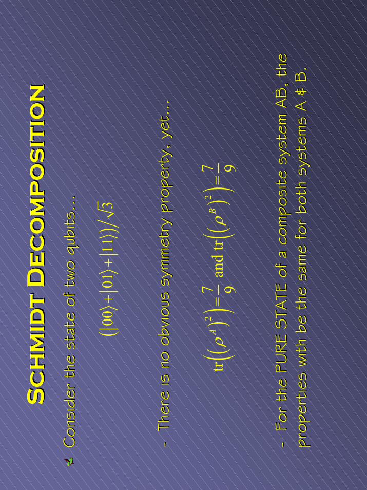
Sc
hm
idt
De
co
mp
os
itio
nS
ch
mid
t D
ec
om
po
sit
ion
Con
side
r th
e st
ate
of t
wo
Con
side
r th
e st
ate
of t
wo
qubi
tsqu
bits
……
--Th
ere
is n
o ob
viou
s sy
mm
etry
pro
pert
y, y
et…
Ther
e is
no
obviou
s sy
mm
etry
pro
pert
y, y
et…
--Fo
r th
e PU
RE
STA
TE o
f a
com
posi
te s
yste
m A
B, th
e Fo
r th
e PU
RE
STA
TE o
f a
com
posi
te s
yste
m A
B, th
e pr
oper
ties
with
be
the
sam
e fo
r bo
th s
yste
ms
A &
B.
()
0001
113
++
()
()
()
()
22
77
tr=
and
tr=
99
AB
ρρ
prop
ertie
s with
be
the
sam
e fo
r bo
th s
yste
ms
A &
B.
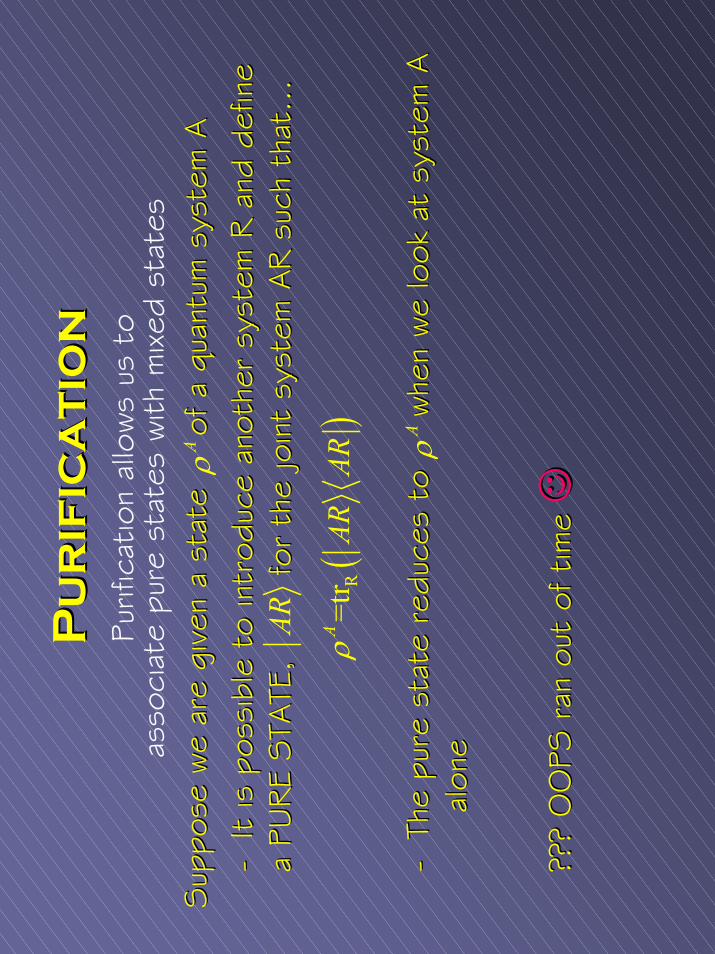
Pu
rif
ica
tio
nP
ur
ific
at
ion
Purif
icat
ion
allo
ws
us t
o as
soci
ate
pure
sta
tes
with
mixed
sta
tes
Sup
pose
we
are
give
n a
stat
e
of
a q
uant
um s
yste
m A
Sup
pose
we
are
give
n a
stat
e
of
a q
uant
um s
yste
m A
--It is
pos
sibl
e to
intr
oduc
e an
othe
r sy
stem
R a
nd d
efin
e It is
pos
sibl
e to
intr
oduc
e an
othe
r sy
stem
R a
nd d
efin
e a
PURE
STA
TE,
for
the
join
t sy
stem
AR s
uch
that
…a
PURE
STA
TE,
for
the
join
t sy
stem
AR s
uch
that
…
--Th
e pu
re s
tate
red
uces
to
whe
n we
look
at
syst
em A
The
pure
sta
te r
educ
es t
o
whe
n we
look
at
syst
em A
alon
eal
one
???
OO
PS r
an o
ut o
f tim
e ??
? O
OPS
ran
out
of tim
e
()
R=t
rA
ARAR
ρ
Aρ
AR
Aρ
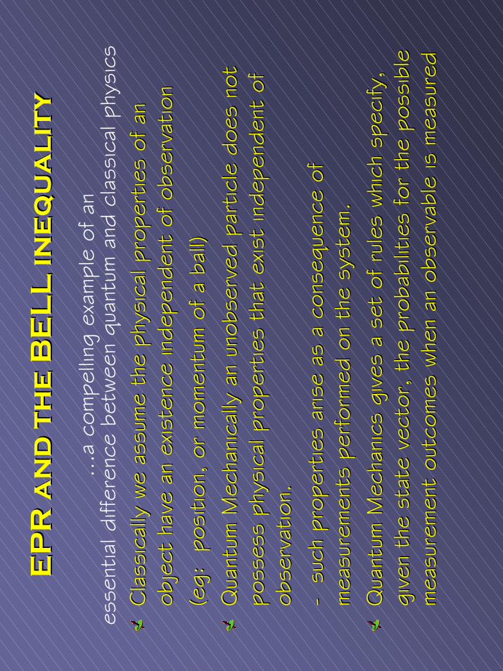
EP
R a
nd
th
e B
EL
L in
eq
ua
lit
yE
PR
an
d t
he
BE
LL
ine
qu
al
ity
…a
com
pelling
exa
mpl
e of
an
esse
ntia
l diff
eren
ce b
etwee
n qu
antu
m a
nd c
lass
ical
phy
sics
Cla
ssic
ally
we
assu
me
the
phys
ical
pro
pert
ies
of a
n C
lass
ical
ly w
e as
sum
e th
e ph
ysic
al p
rope
rtie
s of
an
obje
ct h
ave
an e
xist
ence
inde
pend
ent
of o
bser
vatio
nob
ject
hav
e an
exist
ence
inde
pend
ent
of o
bser
vatio
n(( e
geg:
pos
ition
, or
mom
entu
m o
f a
ball)
: p
ositi
on,
or m
omen
tum
of a
ball)
Qua
ntum
Mec
hani
cally
an
unob
serv
ed p
artic
le d
oes
not
Qua
ntum
Mec
hani
cally
an
unob
serv
ed p
artic
le d
oes
not
poss
ess
phys
ical
pro
pert
ies
that
exist
inde
pend
ent
of
poss
ess
phys
ical
pro
pert
ies
that
exist
inde
pend
ent
of
obse
rvat
ion.
obse
rvat
ion.
--su
ch p
rope
rtie
s ar
ise
as a
con
sequ
ence
of
such
pro
pert
ies
aris
e as
a c
onse
quen
ce o
f m
easu
rem
ents
per
form
ed o
n th
e sy
stem
.m
easu
rem
ents
per
form
ed o
n th
e sy
stem
.Q
uant
um M
echa
nics
gives
a s
et o
f ru
les
whi
ch s
peci
fy,
Qua
ntum
Mec
hani
cs g
ives
a s
et o
f ru
les
whi
ch s
peci
fy,
give
n th
e st
ate
vect
or,
the
prob
abilitie
s fo
r th
e po
ssib
le
give
n th
e st
ate
vect
or,
the
prob
abilitie
s fo
r th
e po
ssib
le
mea
sure
men
t ou
tcom
es w
hen
an o
bser
vabl
e is
mea
sure
dm
easu
rem
ent
outc
omes
whe
n an
obs
erva
ble
is m
easu
red
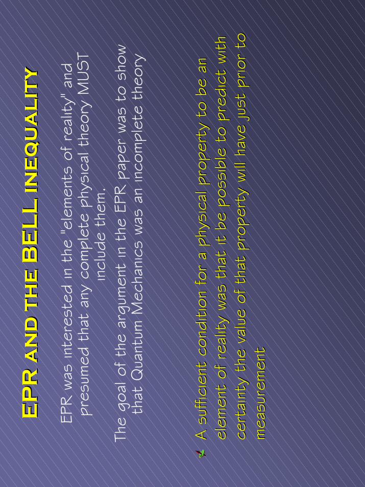
EP
R a
nd
th
e B
EL
L in
eq
ua
lit
yE
PR
an
d t
he
BE
LL
ine
qu
al
ity
EPR w
as in
tere
sted
in t
he "e
lem
ents
of re
ality
" and
pr
esum
ed t
hat
any
com
plet
e ph
ysic
al t
heor
y M
UST
incl
ude
them
.
The
goal
of th
e ar
gum
ent
in t
he E
PR p
aper
was
to
show
th
at Q
uant
um M
echa
nics
was
an
inco
mpl
ete
theo
ry
A s
uffic
ient
con
ditio
n fo
r a
phys
ical
pro
pert
y to
be
an
A s
uffic
ient
con
ditio
n fo
r a
phys
ical
pro
pert
y to
be
an
elem
ent
of r
ealit
y was
tha
t it
be p
ossi
ble
to p
redi
ct w
ith
elem
ent
of r
ealit
y was
tha
t it
be p
ossi
ble
to p
redi
ct w
ith
cert
aint
y th
e va
lue
of t
hat
prop
erty
will h
ave
just
prio
r to
ce
rtai
nty
the
valu
e of
tha
t pr
oper
ty w
ill h
ave
just
prio
r to
m
easu
rem
ent
mea
sure
men
t
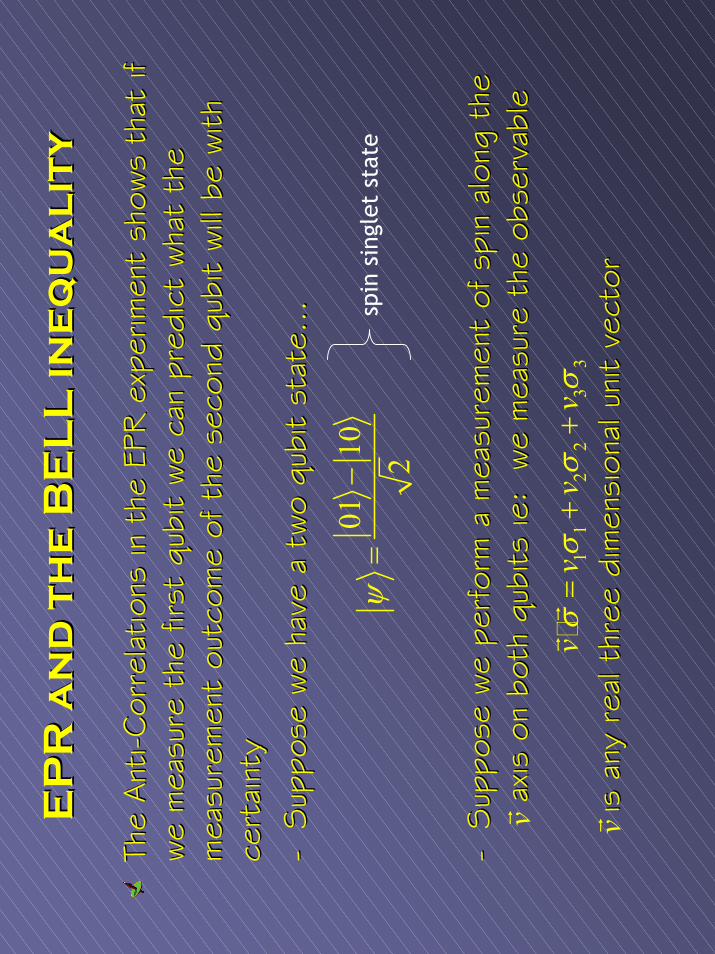
EP
R a
nd
th
e B
EL
L in
eq
ua
lit
yE
PR
an
d t
he
BE
LL
ine
qu
al
ity
The
Ant
iTh
e Ant
i --C
orre
latio
ns in
the
EPR
exp
erim
ent
show
s th
at if
C
orre
latio
ns in
the
EPR
exp
erim
ent
show
s th
at if
we
mea
sure
the
firs
t we
mea
sure
the
firs
t qu
bit
qubi
twe
can
pred
ict
wha
t th
e we
can
pred
ict
wha
t th
e m
easu
rem
ent
outc
ome
of t
he s
econ
d m
easu
rem
ent
outc
ome
of t
he s
econ
d qu
bit
qubi
twill b
e with
will b
e with
ce
rtai
nty
cert
aint
y--
Sup
pose
we
have
a t
wo
Sup
pose
we
have
a t
wo
qubi
tqu
bit
stat
e…st
ate…
--Sup
pose
we
perfor
m a
mea
sure
men
t of
spi
n al
ong
the
Sup
pose
we
perfor
m a
mea
sure
men
t of
spi
n al
ong
the
axis
on
both
ax
is o
n bo
th q
ubits
qubi
tsieie
: w
e m
easu
re t
he o
bser
vabl
e: w
e m
easu
re t
he o
bser
vabl
e
is a
ny r
eal t
hree
dim
ensi
onal
uni
t ve
ctor
is a
ny r
eal t
hree
dim
ensi
onal
uni
t ve
ctor
0110 2
ψ−
=sp
in s
ingl
etst
ate
11
22
33
vv
vv
σσ
σσ
=+
+rr
vr vr

EP
R a
nd
th
e B
EL
L in
eq
ua
lit
yE
PR
an
d t
he
BE
LL
ine
qu
al
ity
[mor
e to
com
e][m
ore
to c
ome]
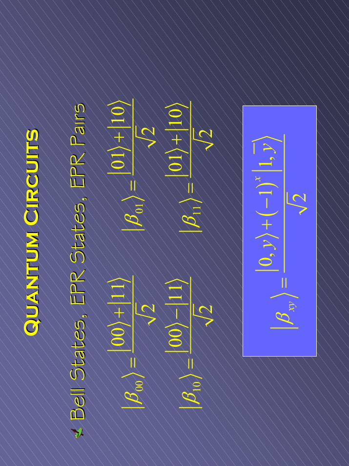
Qu
an
tu
m C
irc
uit
sQ
ua
nt
um
Cir
cu
its
Bel
l Sta
tes,
EPR
Sta
tes,
EPR
Pai
rsBel
l Sta
tes,
EPR
Sta
tes,
EPR
Pai
rs
0001
1011
0011
0110
2
200
1101
10
22
ββ
ββ
++
==
−+
==
()
0,1
1,
2
x
xy
yy
β+
−=
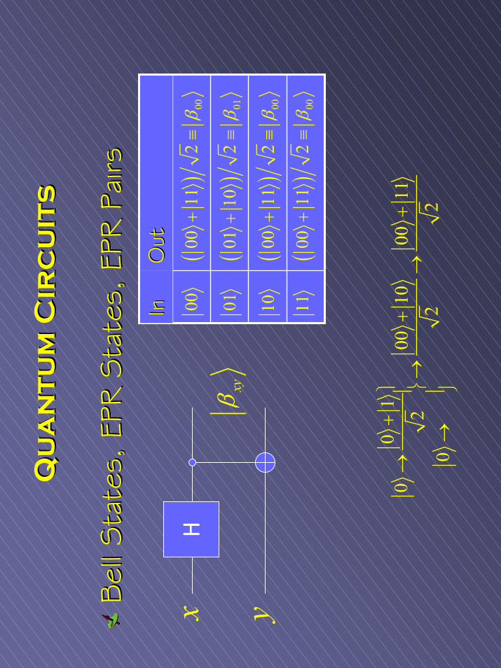
Qu
an
tu
m C
irc
uit
sQ
ua
nt
um
Cir
cu
its
Bel
l Sta
tes,
EPR
Sta
tes,
EPR
Pai
rsBel
l Sta
tes,
EPR
Sta
tes,
EPR
Pai
rs
00 01 10 11
()
0000
112
β+
≡
()
0101
102
β+
≡
()
0000
112
β+
≡
()
0000
112
β+
≡
xH
xyβy
01
000
1000
112
22
0
+
→+
+→
→
→
Out
Out
InIn

()
ii
itrA
iAi
Aψ
ψψ
ψψ
ψ=
=∑
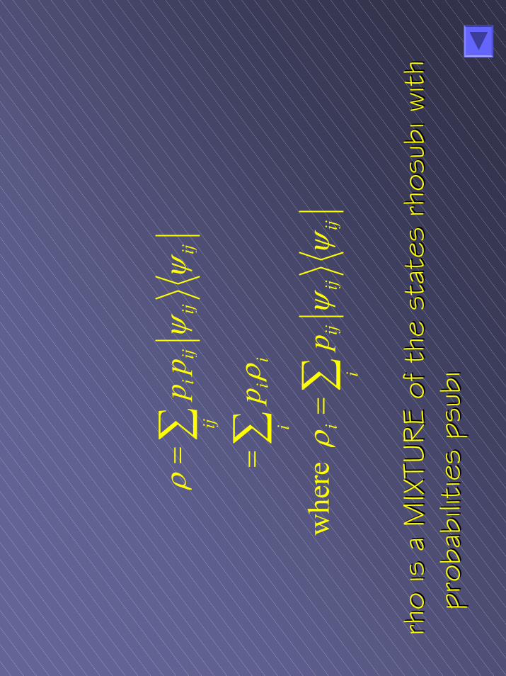
iij
ijij
ij
ii
i
pp
p
ρψ
ψ
ρ
= =
∑ ∑w
here
i
ijij
ijip
ρψ
ψ=∑
rho
rho
is a
MIX
TURE
of t
he s
tate
s is
a M
IXTU
RE
of t
he s
tate
s rh
osub
irh
osub
i with
with
pr
obab
ilitie
s pr
obab
ilitie
s ps
ubi
psub
i
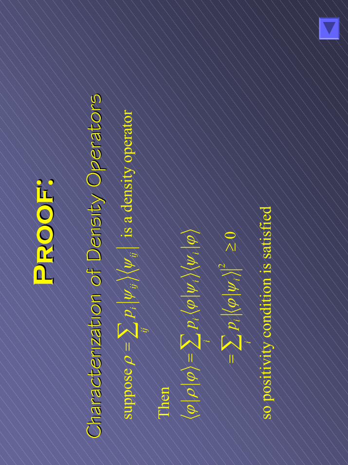
Pr
oo
f:
Pr
oo
f:
Cha
ract
erizat
ion
of D
ensi
ty O
pera
tors
Cha
ract
erizat
ion
of D
ensi
ty O
pera
tors
2
supp
ose
is a
den
sity
ope
rato
r
Then
0
so p
ositi
vity
con
ditio
n is
satis
fied
iij
ijij
ii
ii
ii
i
p
p p
ρψ
ψ
ϕρϕ
ϕψ
ψϕ
ϕψ
=
= =≥
∑ ∑ ∑
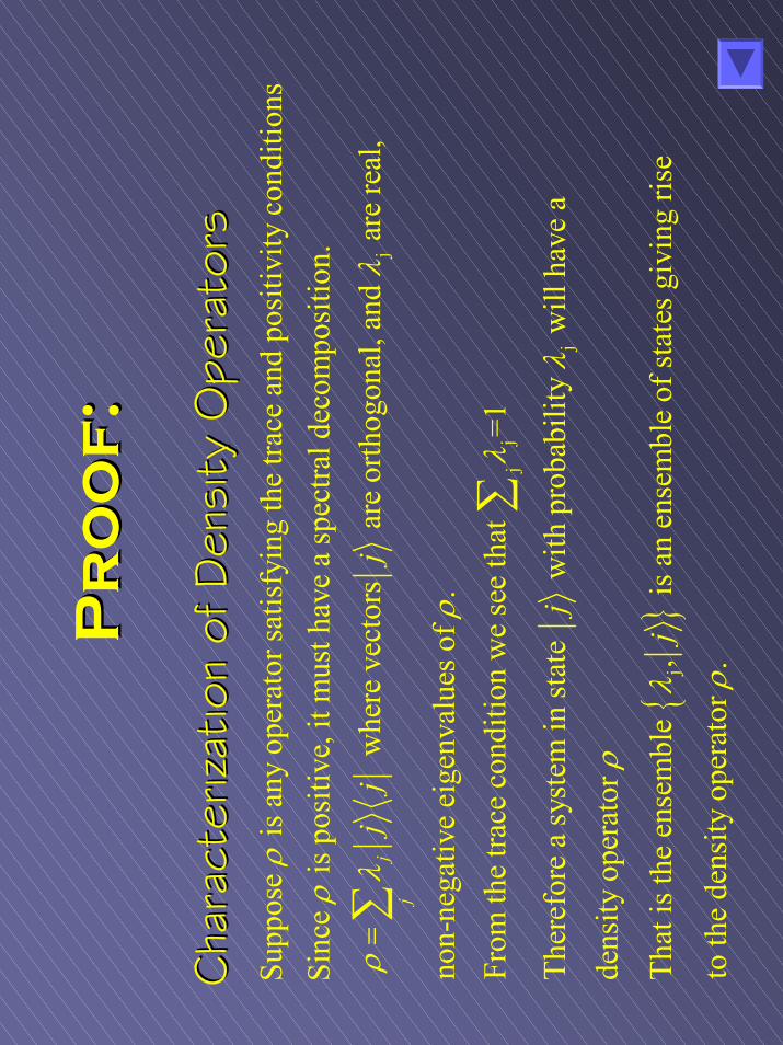
Pr
oo
f:
Pr
oo
f:
Cha
ract
erizat
ion
of D
ensi
ty O
pera
tors
Cha
ract
erizat
ion
of D
ensi
ty O
pera
tors j
Supp
ose
is a
ny o
pera
tor s
atis
fyin
g th
e tra
ce a
nd p
ositi
vity
con
ditio
nsSi
nce
is p
ositi
ve, i
t mus
t hav
e a
spec
tral d
ecom
posi
tion.
w
here
vec
tors
are
orth
ogon
al, a
nd
are
real
,
non-
nega
tivjj
jj
j
ρρ
ρλ
λ=∑
jj
j
j
e ei
genv
alue
s of
. Fr
om th
e tra
ce c
ondi
tion
we
see
that
=1
Ther
efor
e a
syst
em in
stat
e w
ith p
roba
bilit
y w
ill h
ave
a
dens
ity o
pera
tor
That
is th
e en
sem
ble
, is
an
ense
mbl
e of
stat
es g
ivin
g
j
j
ρλ
λ
ρ
λ
∑
rise
to th
e de
nsity
ope
rato
r . ρ
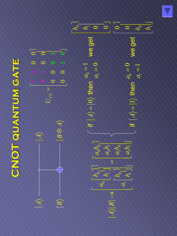
CN
OT
qu
an
tu
m g
at
eC
NO
T q
ua
nt
um
ga
te
A B
A BA
⊕
00
00
00
00
11
0
0 0
1 01
CN
U
=
0
01
01
00
01
01
10
01
11
01
10 1
1
0
0
0 0
00
0
1
1
ba
bA
ba
ab
ab
ab
AB
ab
ba
ab
ab
Aa
b b
=
=
=
→
=
=
=
=
ifth
enw
e ge
t
ifth
enw
e ge
t
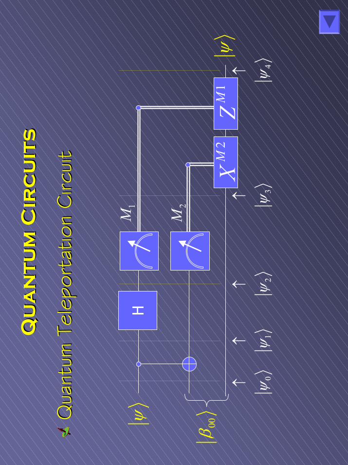
Qu
an
tu
m C
irc
uit
sQ
ua
nt
um
Cir
cu
its
Qua
ntum
Tel
epor
tatio
n Circ
uit
Qua
ntum
Tel
epor
tatio
n Circ
uit
H
ψ
1M
2M
2M
X1
MZ
ψ 00β
0ψ↑
1ψ↑
2ψ↑
3ψ↑
4ψ↑
1
Quantum Computing Summer School
Lecture 3: Postulates of Lecture 3: Postulates of Quantum MechanicsQuantum Mechanics
Angela AntoniuAngela AntoniuDepartment of Electrical and Department of Electrical and Computing EngineeringComputing Engineering
May 9, 2002May 9, 2002
Postulates of Quantum MechanicsPostulates of Quantum MechanicsLecture objectivesLecture objectives
Why are postulates important?Why are postulates important?… they provide the … they provide the connectionsconnections between the between the physical, real, world and the quantum physical, real, world and the quantum mechanics mathematics used to model these mechanics mathematics used to model these systemssystems
Lecture ObjectivesLecture ObjectivesDescription of connectionsDescription of connectionsIntroduce the postulatesIntroduce the postulatesLearn how to use themLearn how to use them…and when to use them…and when to use them
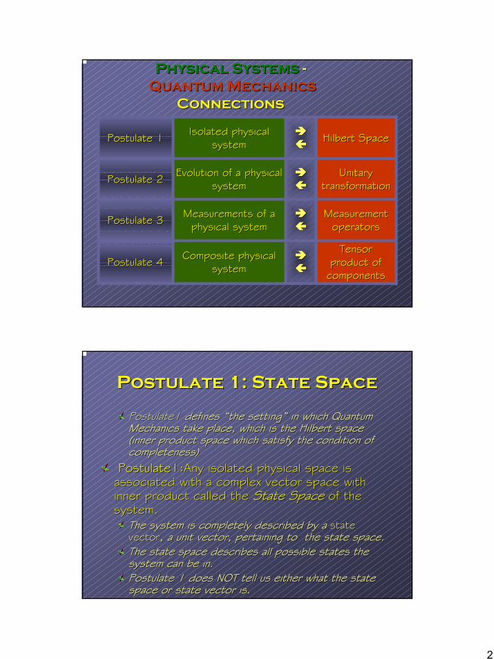
2
Physical SystemsPhysical Systems --Quantum MechanicsQuantum Mechanics
ConnectionsConnections
Tensor Tensor product of product of componentscomponents
Composite physical Composite physical systemsystemPostulate 4Postulate 4
Measurement Measurement operatorsoperators
Measurements of a Measurements of a physical systemphysical systemPostulate 3Postulate 3
Unitary Unitary transformationtransformation
Evolution of a physical Evolution of a physical systemsystemPostulate 2Postulate 2
Hilbert SpaceHilbert SpaceIsolated physical Isolated physical systemsystemPostulate 1Postulate 1
Postulate 1: State SpacePostulate 1: State Space
Postulate1 Postulate1 defines “the setting” in which Quantum defines “the setting” in which Quantum Mechanics take place, which is the Hilbert space Mechanics take place, which is the Hilbert space (inner product space which satisfy the condition of (inner product space which satisfy the condition of completeness)completeness)
Postulate1:Postulate1:Any isolatedAny isolated physical space is physical space is associated with a complex vector space with associated with a complex vector space with inner product called the inner product called the State SpaceState Space of the of the system. system.
The system is completely described by a The system is completely described by a state state vectorvector, a unit vector, pertaining to the state space. , a unit vector, pertaining to the state space. The state space describes all possible states the The state space describes all possible states the system can be in. system can be in. Postulate 1 does NOT tell us either what the state Postulate 1 does NOT tell us either what the state space or state vector is.space or state vector is.
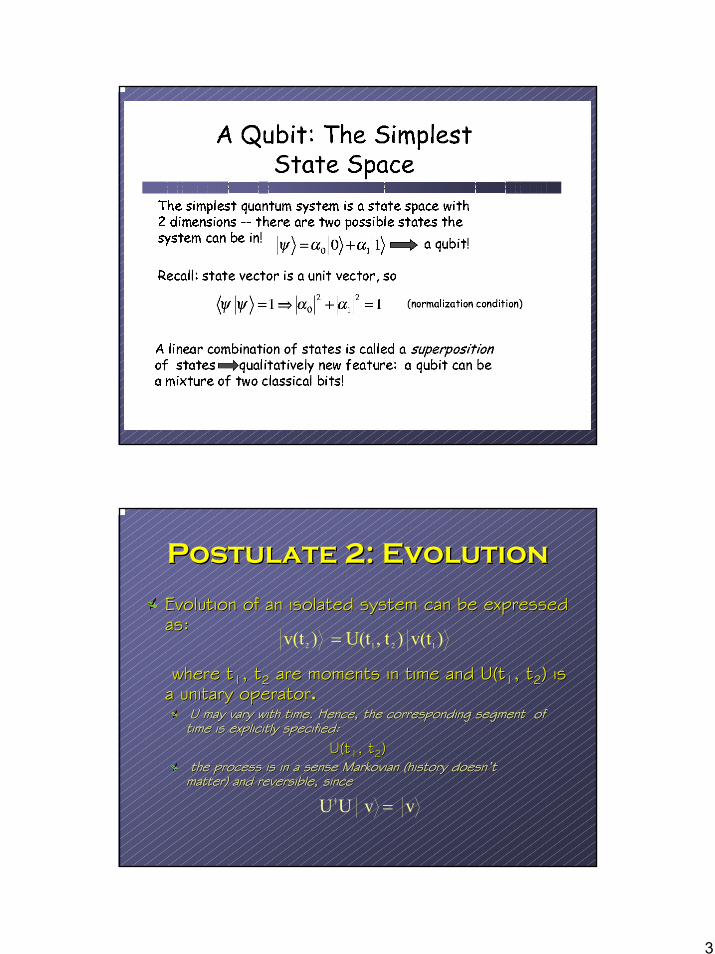
3
Postulate 2: EvolutionPostulate 2: Evolution
Evolution of an isolated system can be expressed Evolution of an isolated system can be expressed as:as:
where twhere t11, t, t22 are moments in time and U(tare moments in time and U(t11, t, t22) is ) is a unitary operatora unitary operator..
U may vary with time. Hence, the corresponding segment of U may vary with time. Hence, the corresponding segment of time is explicitly specified:time is explicitly specified:
U(tU(t11, t, t22))the process is in a sensethe process is in a sense MarkovianMarkovian (history doesn’t (history doesn’t matter) and reversible, since matter) and reversible, since
)v(t)t,U(t )v(t 1212 =
v vUU† =
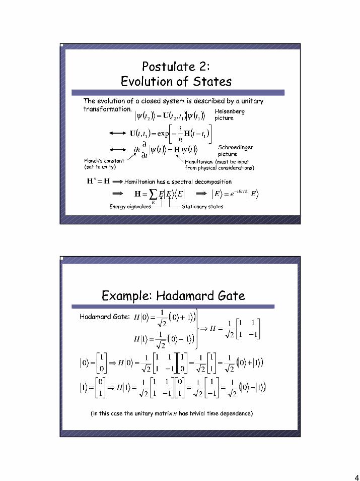
4
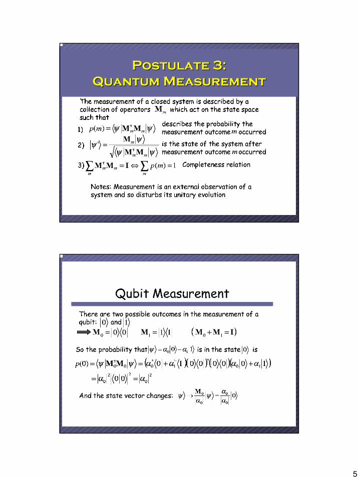
5
Postulate 3: Postulate 3: Quantum MeasurementQuantum Measurement
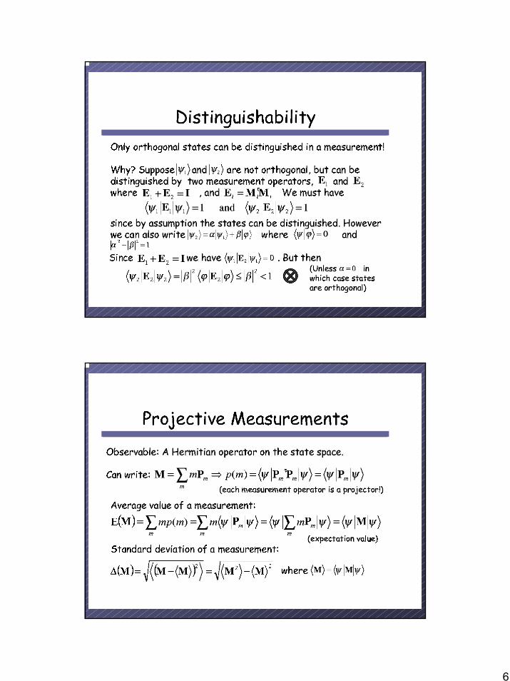
6
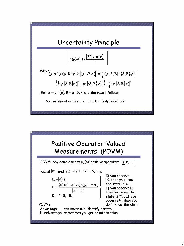
7
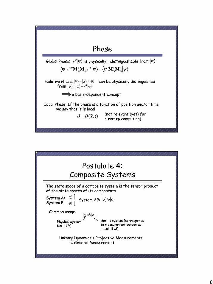
8
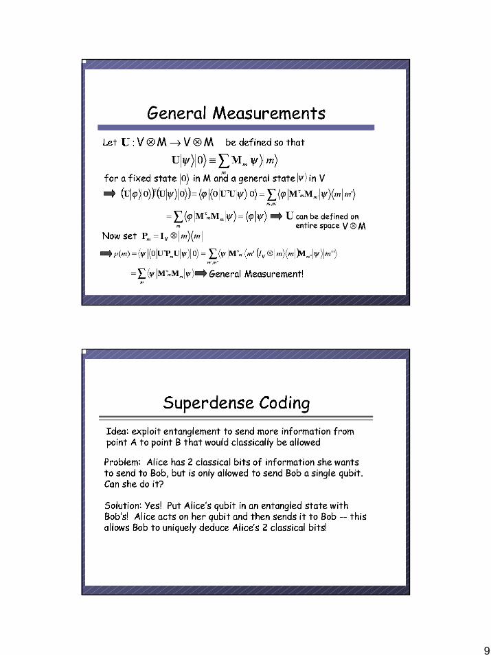
9
10
Bibliography & Bibliography & acknowledgementsacknowledgements
Michael A. Nielsen and Isaac L. Chuang, Quantum Computation and Quantum Information, Cambridge University Press, Cambridge, UK, 2002 V. Bulitko, On quantum Computing and AI, Notes for a graduate class, University of Alberta, 2002R. Mann,M.Mosca, Introduction to Quantum Computation, Lecture series, Univ. Waterloo, 2000 http://cacr.math.uwaterloo.ca/~mmosca/quantumcoursef00.htm D. Fotin, Introduction to “Quantum Computing Summer School”, University of Alberta, 2002.
1
Quantum Computing Quantum Computing Summer SchoolSummer School
Vadim Bulitko
Lecture 5: EPR, Topics in CS
Presentation OverviewPresentation OverviewPresentation Overview
Super denseSuper denseCodingCoding
EPR & EPR & Bell InequalityBell Inequality
Topics Topics in CSin CS
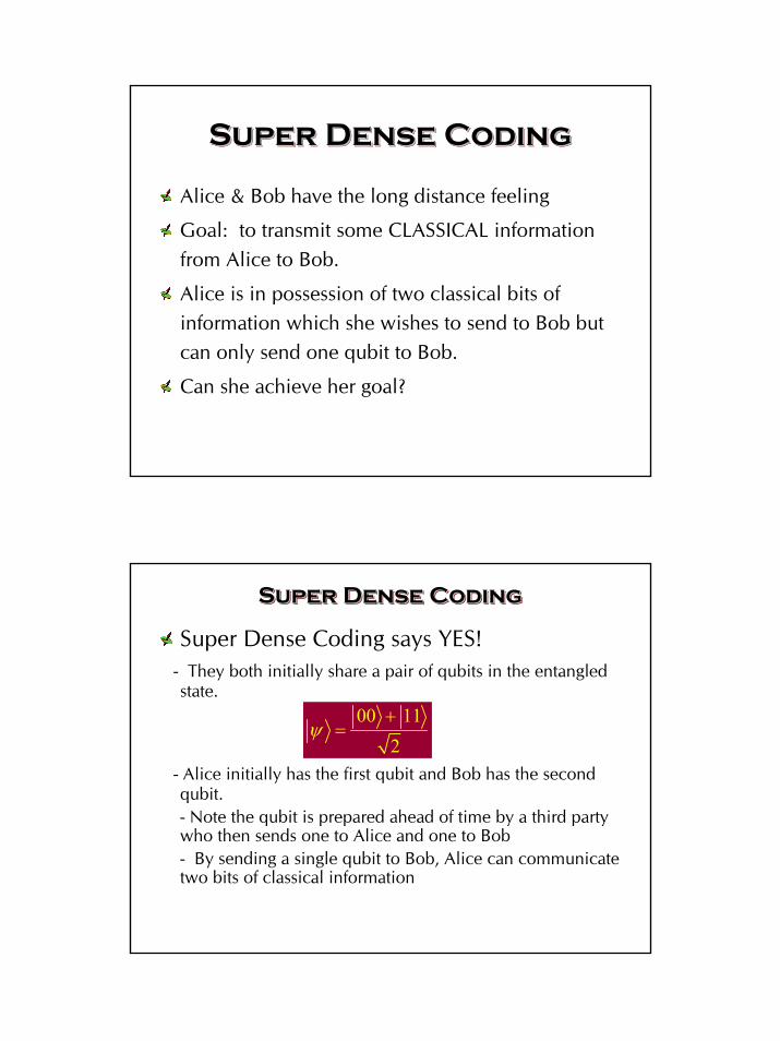
2
Super Dense CodingSuper Dense CodingSuper Dense Coding
Alice & Bob have the long distance feeling
Goal: to transmit some CLASSICAL information from Alice to Bob.
Alice is in possession of two classical bits of information which she wishes to send to Bob but can only send one qubit to Bob.
Can she achieve her goal?
Super Dense CodingSuper Dense CodingSuper Dense Coding
Super Dense Coding says YES!- They both initially share a pair of qubits in the entangled state.
- Alice initially has the first qubit and Bob has the second qubit.- Note the qubit is prepared ahead of time by a third party who then sends one to Alice and one to Bob- By sending a single qubit to Bob, Alice can communicate two bits of classical information
00 112
ψ+
=
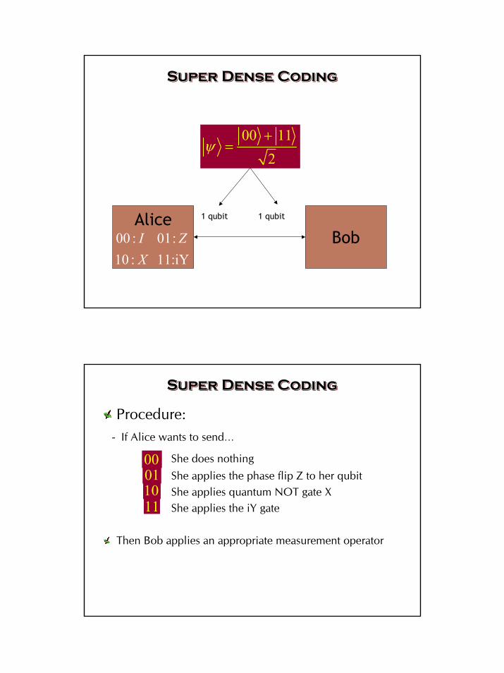
3
Super Dense CodingSuper Dense CodingSuper Dense Coding
00 112
ψ+
=
Alice00 : 01:10 : 11:iY
I ZX
Bob1 qubit 1 qubit
Super Dense CodingSuper Dense CodingSuper Dense Coding
Procedure:- If Alice wants to send…
She does nothingShe applies the phase flip Z to her qubitShe applies quantum NOT gate XShe applies the iY gate
Then Bob applies an appropriate measurement operator
00011011
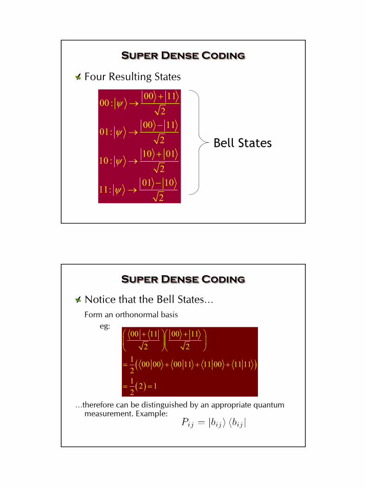
4
Super Dense CodingSuper Dense CodingSuper Dense Coding
Four Resulting States
00 1100 :
200 11
01:2
10 0110 :
201 10
11:2
ψ
ψ
ψ
ψ
+→
−→
+→
−→
Bell States
Super Dense CodingSuper Dense CodingSuper Dense Coding
Notice that the Bell States…Form an orthonormal basis
eg:
…therefore can be distinguished by an appropriate quantum measurement. Example:
( )
( )
00 11 00 112 2
1 00 00 00 11 11 00 11 1121 2 12
+ +
= + + +
= =
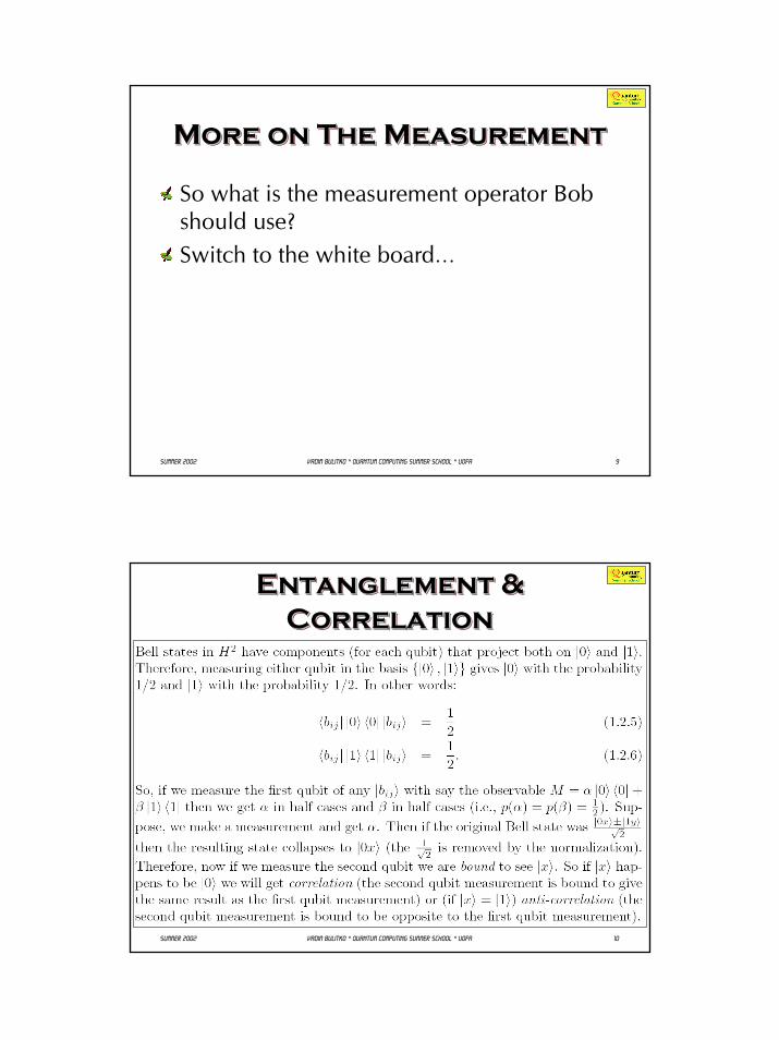
5
99Summer 2002Summer 2002 Vadim Bulitko * Quantum Computing Summer School * UofAVadim Bulitko * Quantum Computing Summer School * UofA
More on The MeasurementMore on The MeasurementMore on The Measurement
So what is the measurement operator Bob should use?Switch to the white board…
1010Summer 2002Summer 2002 Vadim Bulitko * Quantum Computing Summer School * UofAVadim Bulitko * Quantum Computing Summer School * UofA
Entanglement & Correlation
Entanglement & Entanglement & CorrelationCorrelation
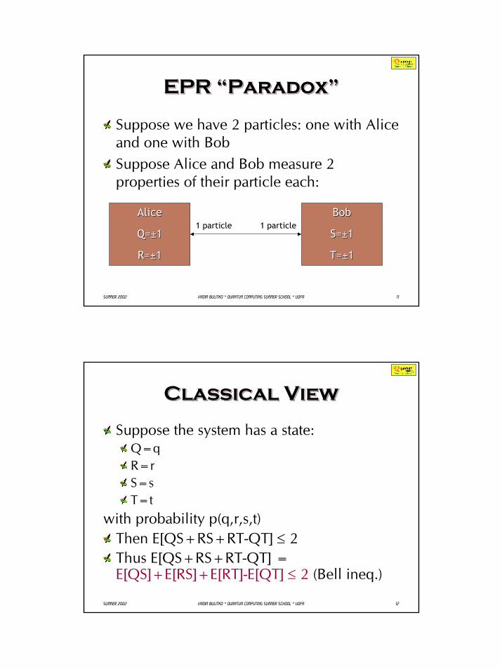
6
1111Summer 2002Summer 2002 Vadim Bulitko * Quantum Computing Summer School * UofAVadim Bulitko * Quantum Computing Summer School * UofA
EPR “Paradox”EPR “Paradox”EPR “Paradox”
Suppose we have 2 particles: one with Alice and one with BobSuppose Alice and Bob measure 2 properties of their particle each:
AliceAlice
Q=±1Q=±1
R=±1R=±1
1 particle 1 particleBobBob
S=±1S=±1
T=±1T=±1
1212Summer 2002Summer 2002 Vadim Bulitko * Quantum Computing Summer School * UofAVadim Bulitko * Quantum Computing Summer School * UofA
Classical ViewClassical ViewClassical View
Suppose the system has a state:Q=qR=rS=sT=t
with probability p(q,r,s,t)Then E[QS+RS+RT-QT] ≤ 2Thus E[QS+RS+RT-QT] = E[QS]+E[RS]+E[RT]-E[QT] ≤ 2 (Bell ineq.)
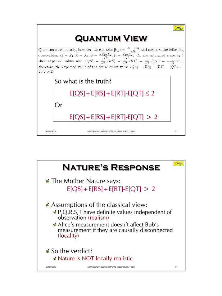
7
1313Summer 2002Summer 2002 Vadim Bulitko * Quantum Computing Summer School * UofAVadim Bulitko * Quantum Computing Summer School * UofA
Quantum ViewQuantum ViewQuantum View
So what is the truth?So what is the truth?
E[QS]+E[RS]+E[RT]E[QS]+E[RS]+E[RT]--E[QT] E[QT] ≤≤ 22
OrOr
E[QS]+E[RS]+E[RT]E[QS]+E[RS]+E[RT]--E[QT] E[QT] > 2> 2
1414Summer 2002Summer 2002 Vadim Bulitko * Quantum Computing Summer School * UofAVadim Bulitko * Quantum Computing Summer School * UofA
Nature’s ResponseNature’s ResponseNature’s ResponseThe Mother Nature says:
E[QS]+E[RS]+E[RT]-E[QT] > 2
Assumptions of the classical view:P,Q,R,S,T have definite values independent of observation (realism)Alice’s measurement doesn’t affect Bob’s measurement if they are causally disconnected (locality)
So the verdict?Nature is NOT locally realistic
8
1515Summer 2002Summer 2002 Vadim Bulitko * Quantum Computing Summer School * UofAVadim Bulitko * Quantum Computing Summer School * UofA
Does The Reality Exist?Does The Reality Exist?Does The Reality Exist?
I recall that during one walk Einstein suddenly stopped, turned to me and asked whether I really believed that the moon exists only when I look at it.
Abraham Pais
1616Summer 2002Summer 2002 Vadim Bulitko * Quantum Computing Summer School * UofAVadim Bulitko * Quantum Computing Summer School * UofA
Computer ScienceComputer ScienceComputer Science
Goal: Brush up on CS aspects relevant to QCModels of computation:
Turing machinesCircuits
Computation problemsDescriptionAlgorithmsComplexity : asymptotic notationComplexity : classes
Energy & computation : reversibility
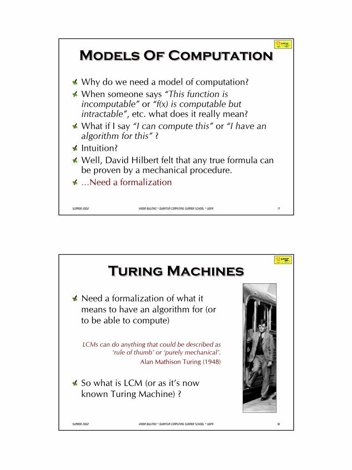
9
1717Summer 2002Summer 2002 Vadim Bulitko * Quantum Computing Summer School * UofAVadim Bulitko * Quantum Computing Summer School * UofA
Models Of ComputationModels Of ComputationModels Of Computation
Why do we need a model of computation?When someone says “This function is incomputable” or “f(x) is computable but intractable”, etc. what does it really mean?What if I say “I can compute this” or “I have an algorithm for this” ?Intuition?Well, David Hilbert felt that any true formula can be proven by a mechanical procedure. …Need a formalization
1818Summer 2002Summer 2002 Vadim Bulitko * Quantum Computing Summer School * UofAVadim Bulitko * Quantum Computing Summer School * UofA
Turing MachinesTuring MachinesTuring Machines
Need a formalization of what it means to have an algorithm for (or to be able to compute)
LCMs can do anything that could be described as ‘rule of thumb’ or ‘purely mechanical’.
Alan Mathison Turing (1948)
So what is LCM (or as it’s now known Turing Machine) ?
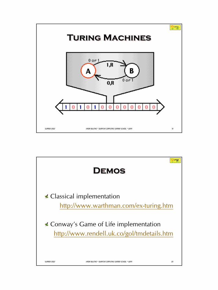
10
1919Summer 2002Summer 2002 Vadim Bulitko * Quantum Computing Summer School * UofAVadim Bulitko * Quantum Computing Summer School * UofA
Turing MachinesTuring MachinesTuring Machines
2020Summer 2002Summer 2002 Vadim Bulitko * Quantum Computing Summer School * UofAVadim Bulitko * Quantum Computing Summer School * UofA
DemosDemosDemos
Classical implementationhttp://www.warthman.com/ex-turing.htm
Conway’s Game of Life implementationhttp://www.rendell.uk.co/gol/tmdetails.htm
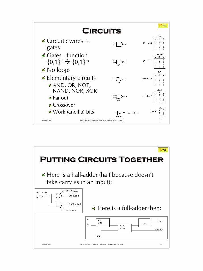
11
2121Summer 2002Summer 2002 Vadim Bulitko * Quantum Computing Summer School * UofAVadim Bulitko * Quantum Computing Summer School * UofA
CircuitsCircuitsCircuitsCircuit : wires + gatesGates : function 0,1k 0,1m
No loopsElementary circuits
AND, OR, NOT, NAND, NOR, XORFanoutCrossoverWork (ancilla) bits
2222Summer 2002Summer 2002 Vadim Bulitko * Quantum Computing Summer School * UofAVadim Bulitko * Quantum Computing Summer School * UofA
Putting Circuits TogetherPutting Circuits TogetherPutting Circuits Together
Here is a half-adder (half because doesn’t take carry as in an input):
Here is a full-adder then:
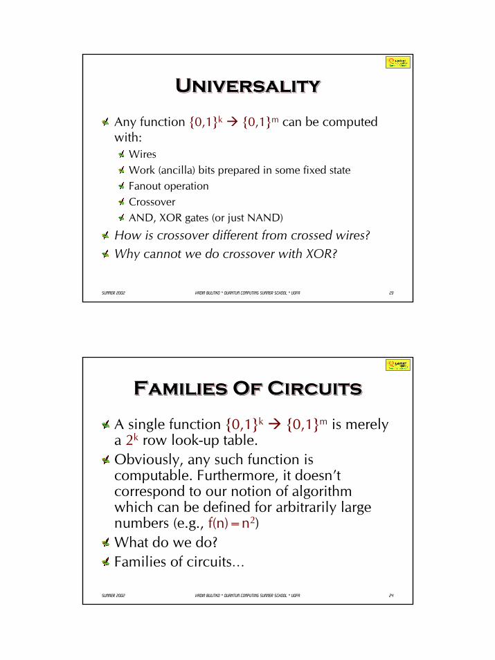
12
2323Summer 2002Summer 2002 Vadim Bulitko * Quantum Computing Summer School * UofAVadim Bulitko * Quantum Computing Summer School * UofA
UniversalityUniversalityUniversality
Any function 0,1k 0,1m can be computed with:
WiresWork (ancilla) bits prepared in some fixed stateFanout operationCrossoverAND, XOR gates (or just NAND)
How is crossover different from crossed wires?Why cannot we do crossover with XOR?
2424Summer 2002Summer 2002 Vadim Bulitko * Quantum Computing Summer School * UofAVadim Bulitko * Quantum Computing Summer School * UofA
Families Of CircuitsFamilies Of CircuitsFamilies Of Circuits
A single function 0,1k 0,1m is merely a 2k row look-up table. Obviously, any such function is computable. Furthermore, it doesn’t correspond to our notion of algorithm which can be defined for arbitrarily large numbers (e.g., f(n)=n2)What do we do?Families of circuits…
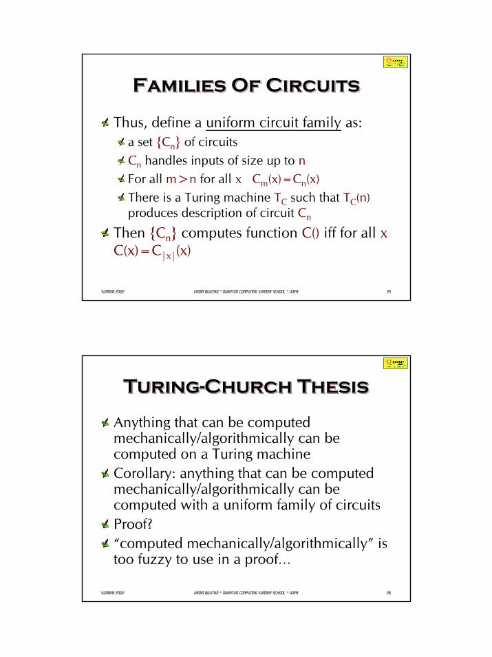
13
2525Summer 2002Summer 2002 Vadim Bulitko * Quantum Computing Summer School * UofAVadim Bulitko * Quantum Computing Summer School * UofA
Families Of CircuitsFamilies Of CircuitsFamilies Of Circuits
Thus, define a uniform circuit family as: a set Cn of circuits Cn handles inputs of size up to nFor all m>n for all x Cm(x)=Cn(x)There is a Turing machine TC such that TC(n)produces description of circuit Cn
Then Cn computes function C() iff for all xC(x)=C|x|(x)
2626Summer 2002Summer 2002 Vadim Bulitko * Quantum Computing Summer School * UofAVadim Bulitko * Quantum Computing Summer School * UofA
Turing-Church ThesisTuringTuring--Church ThesisChurch Thesis
Anything that can be computed mechanically/algorithmically can be computed on a Turing machineCorollary: anything that can be computed mechanically/algorithmically can be computed with a uniform family of circuitsProof?“computed mechanically/algorithmically” is too fuzzy to use in a proof…
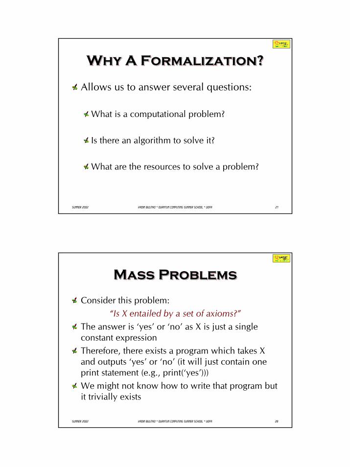
14
2727Summer 2002Summer 2002 Vadim Bulitko * Quantum Computing Summer School * UofAVadim Bulitko * Quantum Computing Summer School * UofA
Why A Formalization?Why A Formalization?Why A Formalization?
Allows us to answer several questions:
What is a computational problem?
Is there an algorithm to solve it?
What are the resources to solve a problem?
2828Summer 2002Summer 2002 Vadim Bulitko * Quantum Computing Summer School * UofAVadim Bulitko * Quantum Computing Summer School * UofA
Mass ProblemsMass ProblemsMass Problems
Consider this problem:“Is X entailed by a set of axioms?”
The answer is ‘yes’ or ‘no’ as X is just a single constant expressionTherefore, there exists a program which takes X and outputs ‘yes’ or ‘no’ (it will just contain one print statement (e.g., print(‘yes’)))We might not know how to write that program but it trivially exists
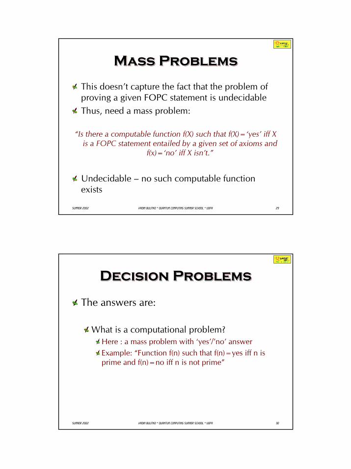
15
2929Summer 2002Summer 2002 Vadim Bulitko * Quantum Computing Summer School * UofAVadim Bulitko * Quantum Computing Summer School * UofA
Mass ProblemsMass ProblemsMass Problems
This doesn’t capture the fact that the problem of proving a given FOPC statement is undecidableThus, need a mass problem:
“Is there a computable function f(X) such that f(X)=‘yes’ iff X is a FOPC statement entailed by a given set of axioms and
f(x)=‘no’ iff X isn’t.”
Undecidable – no such computable function exists
3030Summer 2002Summer 2002 Vadim Bulitko * Quantum Computing Summer School * UofAVadim Bulitko * Quantum Computing Summer School * UofA
Decision ProblemsDecision ProblemsDecision Problems
The answers are:
What is a computational problem?Here : a mass problem with ‘yes’/’no’ answerExample: “Function f(n) such that f(n)=yes iff n is prime and f(n)=no iff n is not prime”
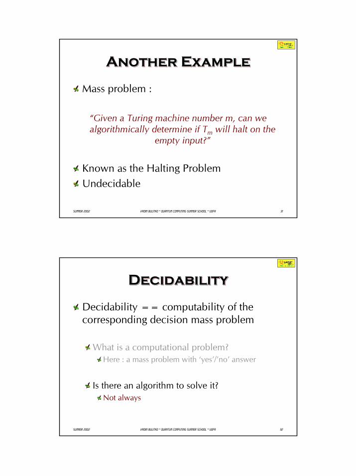
16
3131Summer 2002Summer 2002 Vadim Bulitko * Quantum Computing Summer School * UofAVadim Bulitko * Quantum Computing Summer School * UofA
Another ExampleAnother ExampleAnother Example
Mass problem :
“Given a Turing machine number m, can we algorithmically determine if Tm will halt on the
empty input?”
Known as the Halting ProblemUndecidable
3232Summer 2002Summer 2002 Vadim Bulitko * Quantum Computing Summer School * UofAVadim Bulitko * Quantum Computing Summer School * UofA
DecidabilityDecidabilityDecidability
Decidability == computability of the corresponding decision mass problem
What is a computational problem?Here : a mass problem with ‘yes’/’no’ answer
Is there an algorithm to solve it?Not always
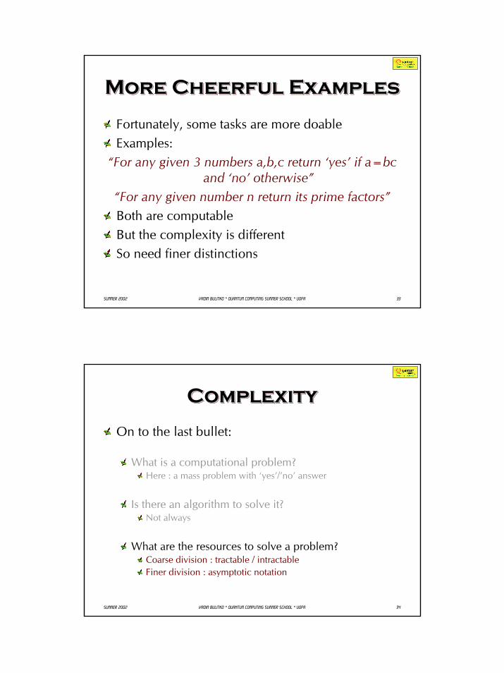
17
3333Summer 2002Summer 2002 Vadim Bulitko * Quantum Computing Summer School * UofAVadim Bulitko * Quantum Computing Summer School * UofA
More Cheerful ExamplesMore Cheerful ExamplesMore Cheerful Examples
Fortunately, some tasks are more doableExamples:
“For any given 3 numbers a,b,c return ‘yes’ if a=bc and ‘no’ otherwise”
“For any given number n return its prime factors”Both are computableBut the complexity is differentSo need finer distinctions
3434Summer 2002Summer 2002 Vadim Bulitko * Quantum Computing Summer School * UofAVadim Bulitko * Quantum Computing Summer School * UofA
ComplexityComplexityComplexity
On to the last bullet:
What is a computational problem?Here : a mass problem with ‘yes’/’no’ answer
Is there an algorithm to solve it?Not always
What are the resources to solve a problem?Coarse division : tractable / intractableFiner division : asymptotic notation
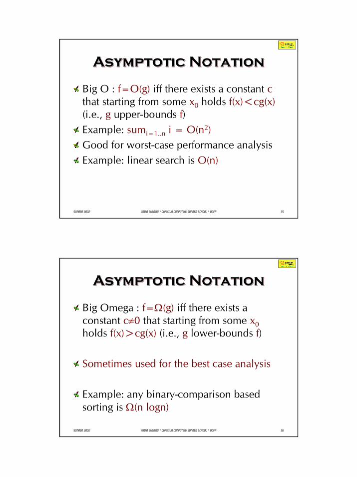
18
3535Summer 2002Summer 2002 Vadim Bulitko * Quantum Computing Summer School * UofAVadim Bulitko * Quantum Computing Summer School * UofA
Asymptotic NotationAsymptotic NotationAsymptotic Notation
Big O : f=O(g) iff there exists a constant cthat starting from some x0 holds f(x)<cg(x)(i.e., g upper-bounds f)Example: sumi=1..n i = O(n2)Good for worst-case performance analysisExample: linear search is O(n)
3636Summer 2002Summer 2002 Vadim Bulitko * Quantum Computing Summer School * UofAVadim Bulitko * Quantum Computing Summer School * UofA
Asymptotic NotationAsymptotic NotationAsymptotic Notation
Big Omega : f=Ω(g) iff there exists a constant c≠0 that starting from some x0holds f(x)>cg(x) (i.e., g lower-bounds f)
Sometimes used for the best case analysis
Example: any binary-comparison based sorting is Ω(n logn)
1
May 21, 2002 University of Alberta * QCSS * Summer 2002 * © Vadim Bulitko 1
QCSS
“Quantum Computing Summer School”
QCSSQCSS
“Quantum Computing “Quantum Computing Summer School”Summer School”
Prof. Vadim BulitkoUniversity of AlbertaProf. Vadim BulitkoProf. Vadim BulitkoUniversity of AlbertaUniversity of Alberta
May 21, 2002 University of Alberta * QCSS * Summer 2002 * © Vadim Bulitko 2
TodayTodayToday
• Computability– Turing-Church thesis
– Turing machines
– Circuits
• Computational complexity– Computable/non-computable
– Asymptotic notation
– P, NP, etc. classes
• Reversibility
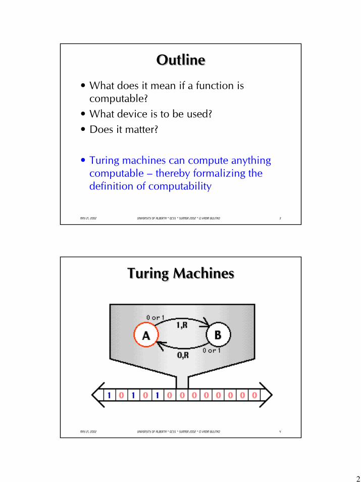
2
May 21, 2002 University of Alberta * QCSS * Summer 2002 * © Vadim Bulitko 3
OutlineOutlineOutline
• What does it mean if a function is computable?
• What device is to be used?• Does it matter?
• Turing machines can compute anything computable – thereby formalizing the definition of computability
May 21, 2002 University of Alberta * QCSS * Summer 2002 * © Vadim Bulitko 4
Turing MachinesTuring MachinesTuring Machines
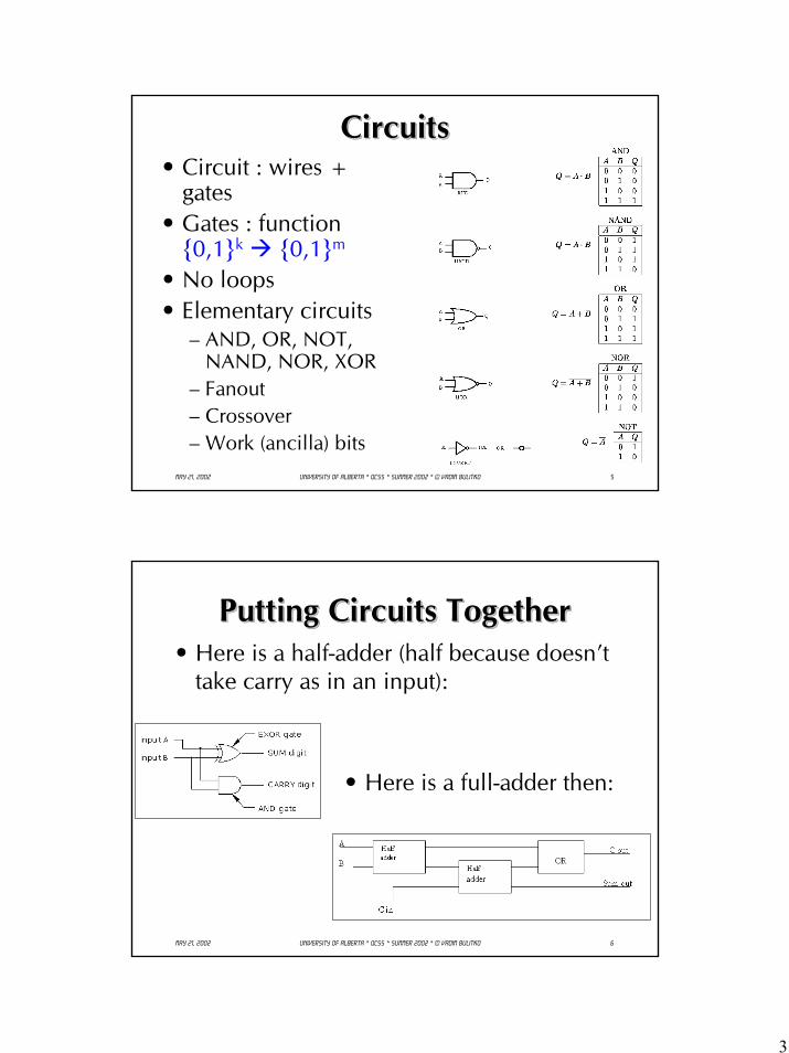
3
May 21, 2002 University of Alberta * QCSS * Summer 2002 * © Vadim Bulitko 5
CircuitsCircuitsCircuits• Circuit : wires +
gates• Gates : function
0,1k 0,1m
• No loops• Elementary circuits
– AND, OR, NOT, NAND, NOR, XOR
– Fanout– Crossover– Work (ancilla) bits
May 21, 2002 University of Alberta * QCSS * Summer 2002 * © Vadim Bulitko 6
Putting Circuits TogetherPutting Circuits TogetherPutting Circuits Together• Here is a half-adder (half because doesn’t
take carry as in an input):
• Here is a full-adder then:
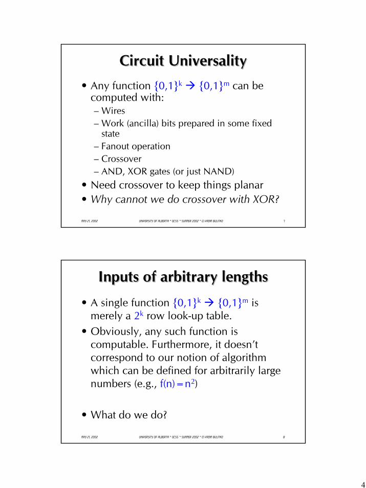
4
May 21, 2002 University of Alberta * QCSS * Summer 2002 * © Vadim Bulitko 7
Circuit UniversalityCircuit UniversalityCircuit Universality
• Any function 0,1k 0,1m can be computed with:– Wires– Work (ancilla) bits prepared in some fixed
state– Fanout operation– Crossover– AND, XOR gates (or just NAND)
• Need crossover to keep things planar• Why cannot we do crossover with XOR?
May 21, 2002 University of Alberta * QCSS * Summer 2002 * © Vadim Bulitko 8
Inputs of arbitrary lengthsInputs of arbitrary lengthsInputs of arbitrary lengths
• A single function 0,1k 0,1m is merely a 2k row look-up table.
• Obviously, any such function is computable. Furthermore, it doesn’t correspond to our notion of algorithm which can be defined for arbitrarily large numbers (e.g., f(n)=n2)
• What do we do?
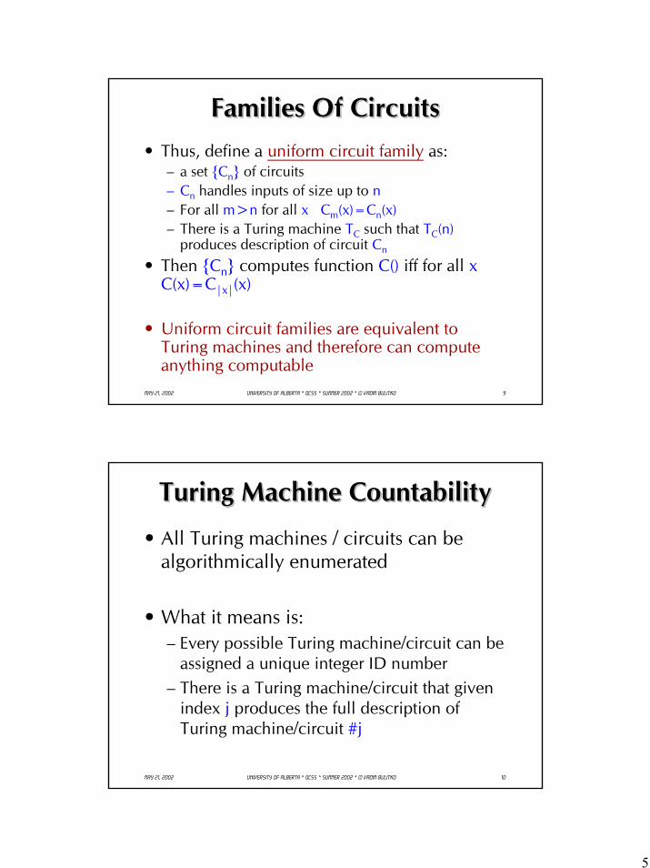
5
May 21, 2002 University of Alberta * QCSS * Summer 2002 * © Vadim Bulitko 9
Families Of CircuitsFamilies Of CircuitsFamilies Of Circuits• Thus, define a uniform circuit family as:
– a set Cn of circuits – Cn handles inputs of size up to n– For all m>n for all x Cm(x)=Cn(x)– There is a Turing machine TC such that TC(n)
produces description of circuit Cn
• Then Cn computes function C() iff for all x C(x)=C|x|(x)
• Uniform circuit families are equivalent to Turing machines and therefore can compute anything computable
May 21, 2002 University of Alberta * QCSS * Summer 2002 * © Vadim Bulitko 10
Turing Machine CountabilityTuring Machine CountabilityTuring Machine Countability
• All Turing machines / circuits can be algorithmically enumerated
• What it means is:– Every possible Turing machine/circuit can be
assigned a unique integer ID number– There is a Turing machine/circuit that given
index j produces the full description of Turing machine/circuit #j
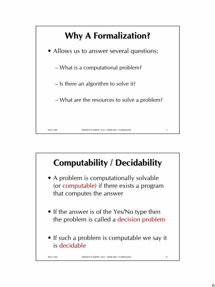
6
May 21, 2002 University of Alberta * QCSS * Summer 2002 * © Vadim Bulitko 11
Why A Formalization?Why A Formalization?Why A Formalization?
• Allows us to answer several questions:
– What is a computational problem?
– Is there an algorithm to solve it?
– What are the resources to solve a problem?
May 21, 2002 University of Alberta * QCSS * Summer 2002 * © Vadim Bulitko 12
Computability / DecidabilityComputability / DecidabilityComputability / Decidability
• A problem is computationally solvable (or computable) if there exists a program that computes the answer
• If the answer is of the Yes/No type then the problem is called a decision problem
• If such a problem is computable we say it is decidable
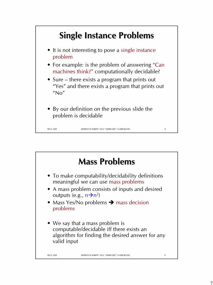
7
May 21, 2002 University of Alberta * QCSS * Summer 2002 * © Vadim Bulitko 13
Single Instance ProblemsSingle Instance ProblemsSingle Instance Problems• It is not interesting to pose a single instance
problem• For example: is the problem of answering “Can
machines think?” computationally decidable?• Sure – there exists a program that prints out
“Yes” and there exists a program that prints out “No”
• By our definition on the previous slide the problem is decidable
May 21, 2002 University of Alberta * QCSS * Summer 2002 * © Vadim Bulitko 14
Mass ProblemsMass ProblemsMass Problems• To make computability/decidability definitions
meaningful we can use mass problems• A mass problem consists of inputs and desired
outputs (e.g., n n2)• Mass Yes/No problems mass decision
problems
• We say that a mass problem is computable/decidable iff there exists an algorithm for finding the desired answer for any valid input
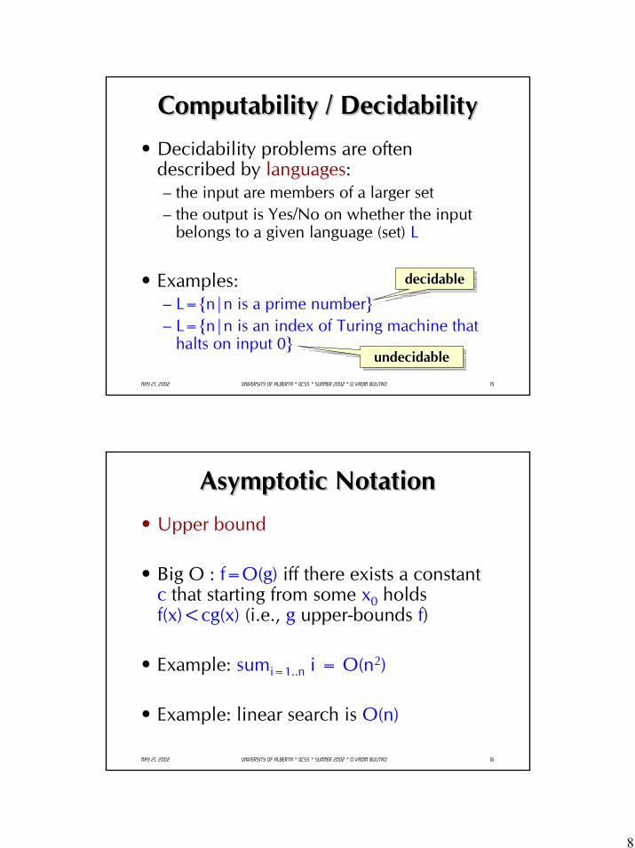
8
May 21, 2002 University of Alberta * QCSS * Summer 2002 * © Vadim Bulitko 15
Computability / DecidabilityComputability / DecidabilityComputability / Decidability
• Decidability problems are often described by languages: – the input are members of a larger set– the output is Yes/No on whether the input
belongs to a given language (set) L
• Examples:– L=n|n is a prime number– L=n|n is an index of Turing machine that
halts on input 0
decidabledecidabledecidable
undecidableundecidableundecidable
May 21, 2002 University of Alberta * QCSS * Summer 2002 * © Vadim Bulitko 16
Asymptotic NotationAsymptotic NotationAsymptotic Notation
• Upper bound
• Big O : f=O(g) iff there exists a constant c that starting from some x0 holds f(x)<cg(x) (i.e., g upper-bounds f)
• Example: sumi=1..n i = O(n2)
• Example: linear search is O(n)
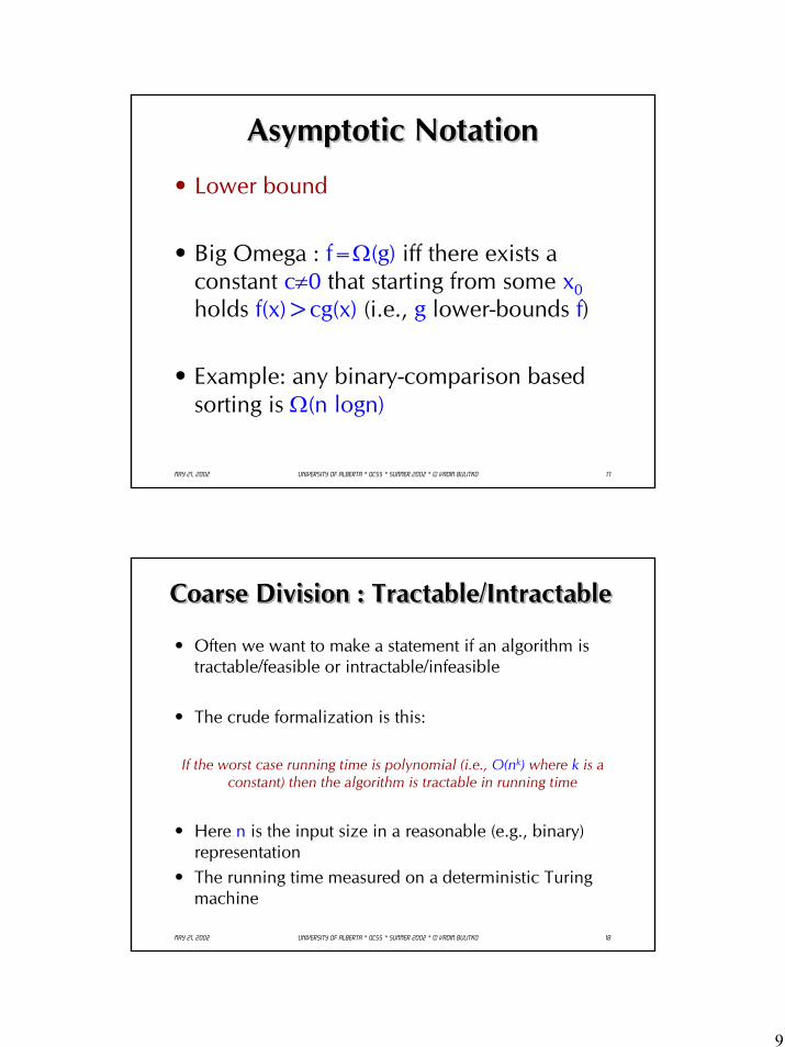
9
May 21, 2002 University of Alberta * QCSS * Summer 2002 * © Vadim Bulitko 17
Asymptotic NotationAsymptotic NotationAsymptotic Notation
• Lower bound
• Big Omega : f=Ω(g) iff there exists a constant c≠0 that starting from some x0holds f(x)>cg(x) (i.e., g lower-bounds f)
• Example: any binary-comparison based sorting is Ω(n logn)
May 21, 2002 University of Alberta * QCSS * Summer 2002 * © Vadim Bulitko 18
Coarse Division : Tractable/IntractableCoarse Division : Tractable/IntractableCoarse Division : Tractable/Intractable
• Often we want to make a statement if an algorithm is tractable/feasible or intractable/infeasible
• The crude formalization is this:
If the worst case running time is polynomial (i.e., O(nk) where k is a constant) then the algorithm is tractable in running time
• Here n is the input size in a reasonable (e.g., binary) representation
• The running time measured on a deterministic Turing machine
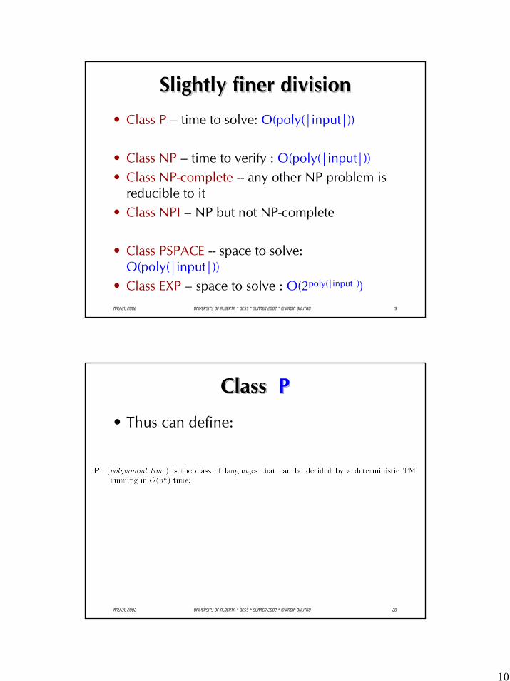
10
May 21, 2002 University of Alberta * QCSS * Summer 2002 * © Vadim Bulitko 19
Slightly finer divisionSlightly finer divisionSlightly finer division• Class P – time to solve: O(poly(|input|))
• Class NP – time to verify : O(poly(|input|))• Class NP-complete -- any other NP problem is
reducible to it• Class NPI – NP but not NP-complete
• Class PSPACE -- space to solve: O(poly(|input|))
• Class EXP – space to solve : O(2poly(|input|))
May 21, 2002 University of Alberta * QCSS * Summer 2002 * © Vadim Bulitko 20
Class PClass Class PP
• Thus can define:
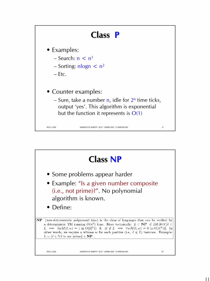
11
May 21, 2002 University of Alberta * QCSS * Summer 2002 * © Vadim Bulitko 21
Class PClass Class PP
• Examples:– Search: n < n1
– Sorting: nlogn < n2
– Etc.
• Counter examples: – Sure, take a number n, idle for 2n time ticks,
output ‘yes’. This algorithm is exponential but the function it represents is O(1)
May 21, 2002 University of Alberta * QCSS * Summer 2002 * © Vadim Bulitko 22
Class NPClass Class NPNP
• Some problems appear harder• Example: “Is a given number composite
(i.e., not prime)?”. No polynomial algorithm is known.
• Define:
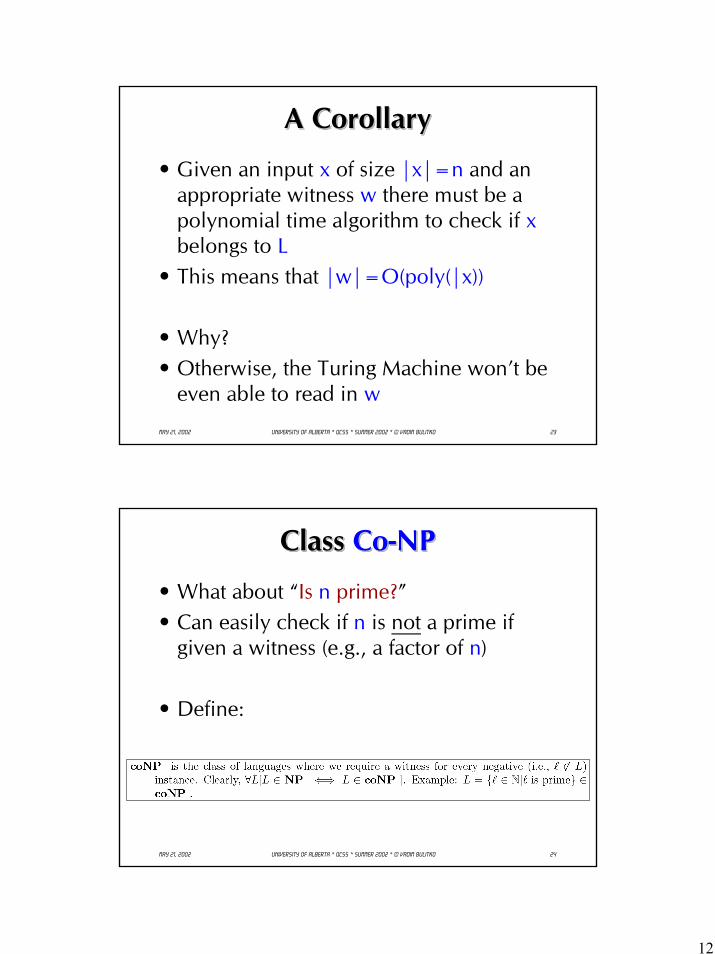
12
May 21, 2002 University of Alberta * QCSS * Summer 2002 * © Vadim Bulitko 23
A CorollaryA CorollaryA Corollary
• Given an input x of size |x|=n and an appropriate witness w there must be a polynomial time algorithm to check if xbelongs to L
• This means that |w|=O(poly(|x))
• Why?• Otherwise, the Turing Machine won’t be
even able to read in w
May 21, 2002 University of Alberta * QCSS * Summer 2002 * © Vadim Bulitko 24
Class Co-NPClass Class CoCo--NPNP
• What about “Is n prime?”• Can easily check if n is not a prime if
given a witness (e.g., a factor of n)
• Define:
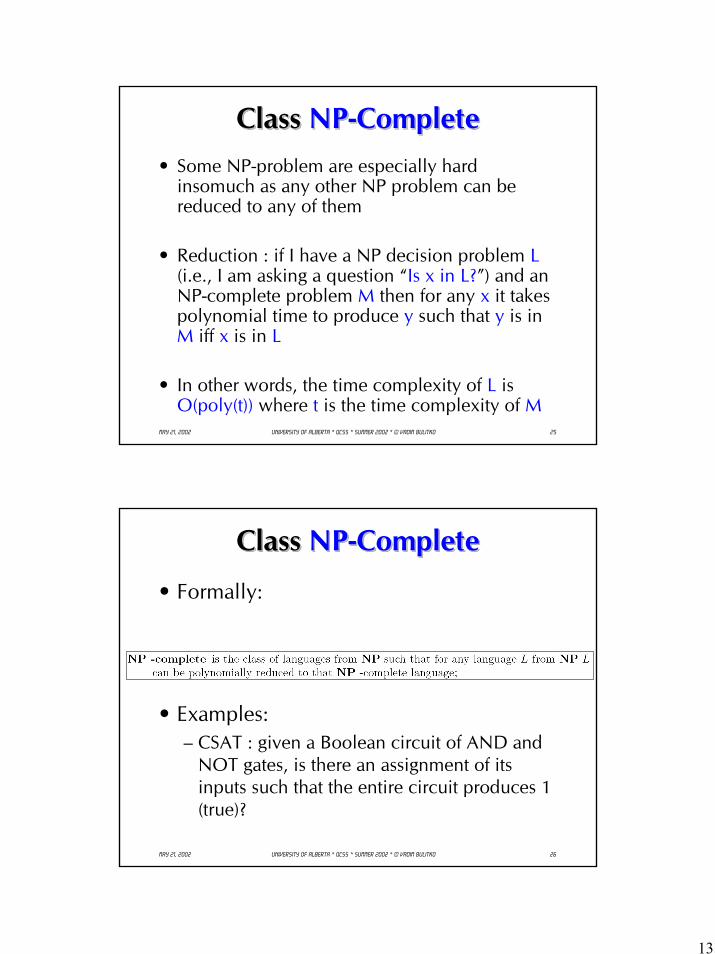
13
May 21, 2002 University of Alberta * QCSS * Summer 2002 * © Vadim Bulitko 25
Class NP-CompleteClass Class NPNP--CompleteComplete• Some NP-problem are especially hard
insomuch as any other NP problem can be reduced to any of them
• Reduction : if I have a NP decision problem L(i.e., I am asking a question “Is x in L?”) and an NP-complete problem M then for any x it takes polynomial time to produce y such that y is in M iff x is in L
• In other words, the time complexity of L is O(poly(t)) where t is the time complexity of M
May 21, 2002 University of Alberta * QCSS * Summer 2002 * © Vadim Bulitko 26
Class NP-CompleteClass Class NPNP--CompleteComplete
• Formally:
• Examples:– CSAT : given a Boolean circuit of AND and
NOT gates, is there an assignment of its inputs such that the entire circuit produces 1 (true)?
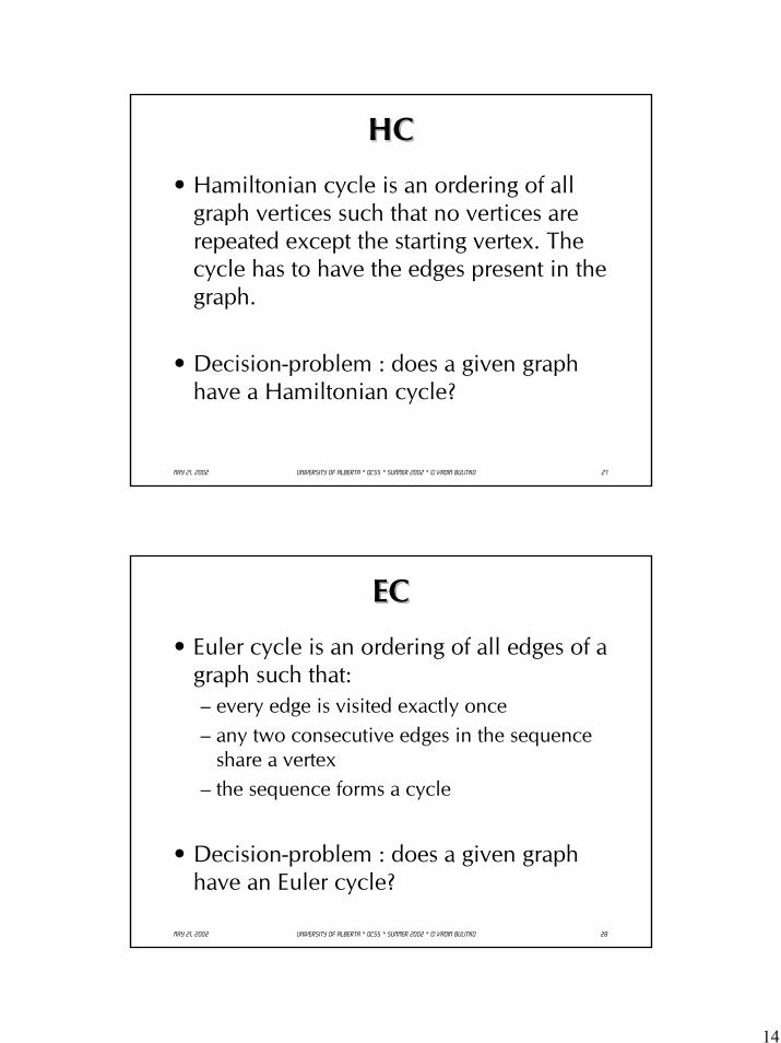
14
May 21, 2002 University of Alberta * QCSS * Summer 2002 * © Vadim Bulitko 27
HCHCHC
• Hamiltonian cycle is an ordering of all graph vertices such that no vertices are repeated except the starting vertex. The cycle has to have the edges present in the graph.
• Decision-problem : does a given graph have a Hamiltonian cycle?
May 21, 2002 University of Alberta * QCSS * Summer 2002 * © Vadim Bulitko 28
ECECEC
• Euler cycle is an ordering of all edges of a graph such that:– every edge is visited exactly once– any two consecutive edges in the sequence
share a vertex– the sequence forms a cycle
• Decision-problem : does a given graph have an Euler cycle?
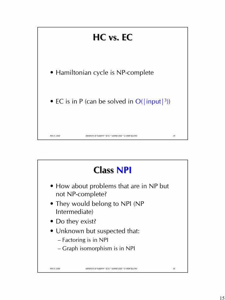
15
May 21, 2002 University of Alberta * QCSS * Summer 2002 * © Vadim Bulitko 29
HC vs. ECHC vs. ECHC vs. EC
• Hamiltonian cycle is NP-complete
• EC is in P (can be solved in O(|input|3))
May 21, 2002 University of Alberta * QCSS * Summer 2002 * © Vadim Bulitko 30
Class NPIClass Class NPINPI
• How about problems that are in NP but not NP-complete?
• They would belong to NPI (NP Intermediate)
• Do they exist?• Unknown but suspected that:
– Factoring is in NPI– Graph isomorphism is in NPI
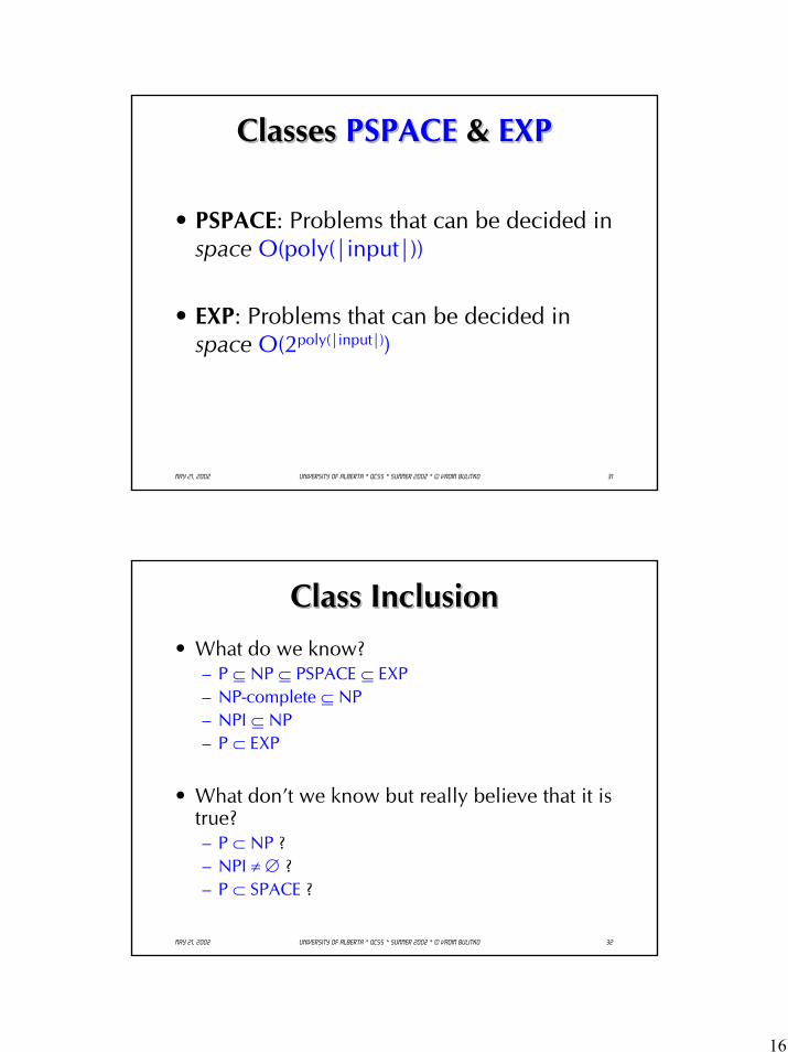
16
May 21, 2002 University of Alberta * QCSS * Summer 2002 * © Vadim Bulitko 31
Classes PSPACE & EXPClasses Classes PSPACEPSPACE & & EXPEXP
• PSPACE: Problems that can be decided in space O(poly(|input|))
• EXP: Problems that can be decided in space O(2poly(|input|))
May 21, 2002 University of Alberta * QCSS * Summer 2002 * © Vadim Bulitko 32
Class InclusionClass InclusionClass Inclusion• What do we know?
– P ⊆ NP ⊆ PSPACE ⊆ EXP– NP-complete ⊆ NP– NPI ⊆ NP– P ⊂ EXP
• What don’t we know but really believe that it is true?– P ⊂ NP ?– NPI ≠ ∅ ? – P ⊂ SPACE ?
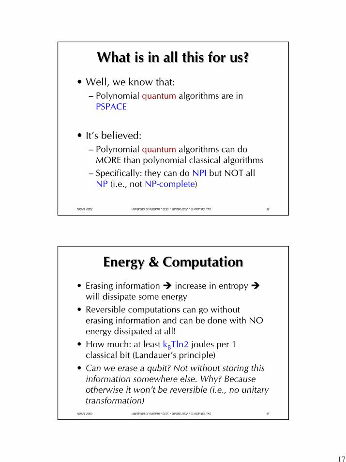
17
May 21, 2002 University of Alberta * QCSS * Summer 2002 * © Vadim Bulitko 33
What is in all this for us?What is in all this for us?What is in all this for us?
• Well, we know that:– Polynomial quantum algorithms are in
PSPACE
• It’s believed:– Polynomial quantum algorithms can do
MORE than polynomial classical algorithms– Specifically: they can do NPI but NOT all
NP (i.e., not NP-complete)
May 21, 2002 University of Alberta * QCSS * Summer 2002 * © Vadim Bulitko 34
Energy & ComputationEnergy & ComputationEnergy & Computation• Erasing information increase in entropy
will dissipate some energy• Reversible computations can go without
erasing information and can be done with NO energy dissipated at all!
• How much: at least kBTln2 joules per 1 classical bit (Landauer’s principle)
• Can we erase a qubit? Not without storing this information somewhere else. Why? Because otherwise it won’t be reversible (i.e., no unitary transformation)
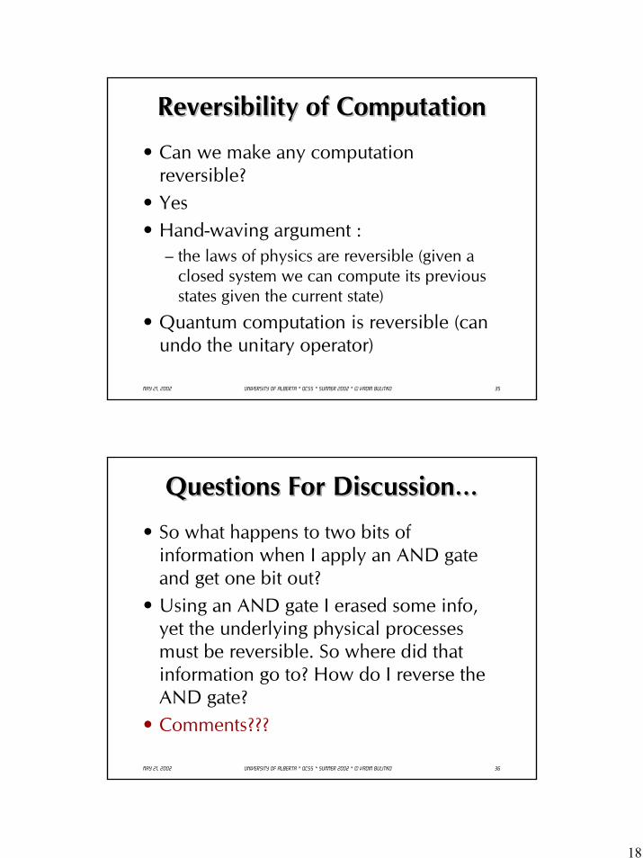
18
May 21, 2002 University of Alberta * QCSS * Summer 2002 * © Vadim Bulitko 35
Reversibility of ComputationReversibility of ComputationReversibility of Computation
• Can we make any computation reversible?
• Yes• Hand-waving argument :
– the laws of physics are reversible (given a closed system we can compute its previous states given the current state)
• Quantum computation is reversible (can undo the unitary operator)
May 21, 2002 University of Alberta * QCSS * Summer 2002 * © Vadim Bulitko 36
Questions For Discussion…Questions For Discussion…Questions For Discussion…
• So what happens to two bits of information when I apply an AND gate and get one bit out?
• Using an AND gate I erased some info, yet the underlying physical processes must be reversible. So where did that information go to? How do I reverse the AND gate?
• Comments???
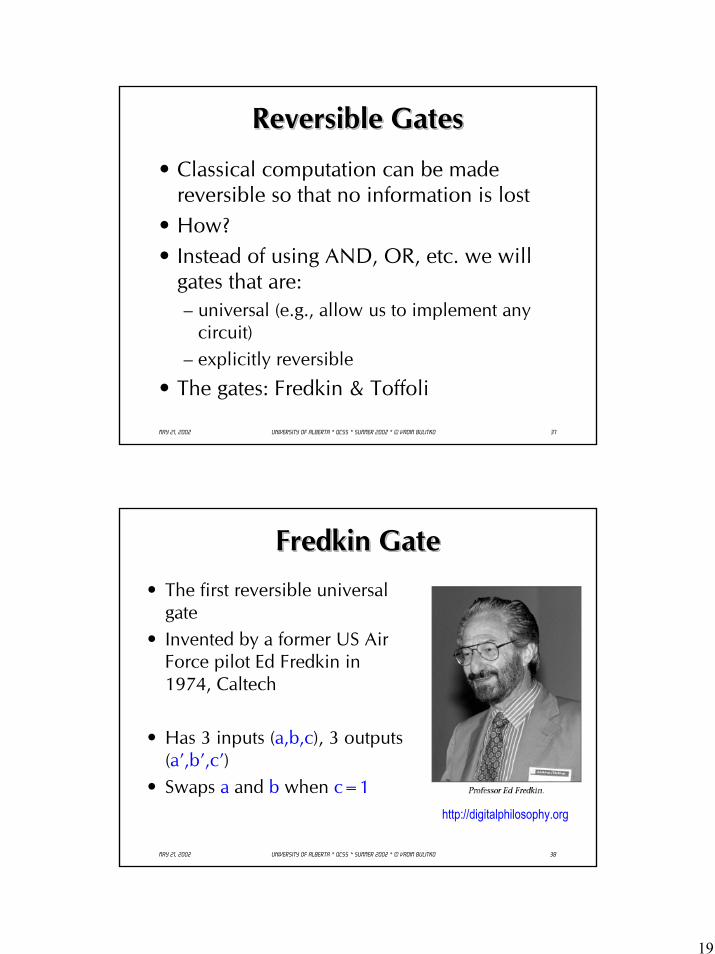
19
May 21, 2002 University of Alberta * QCSS * Summer 2002 * © Vadim Bulitko 37
Reversible GatesReversible GatesReversible Gates
• Classical computation can be made reversible so that no information is lost
• How?• Instead of using AND, OR, etc. we will
gates that are:– universal (e.g., allow us to implement any
circuit)– explicitly reversible
• The gates: Fredkin & Toffoli
May 21, 2002 University of Alberta * QCSS * Summer 2002 * © Vadim Bulitko 38
Fredkin GateFredkin GateFredkin Gate• The first reversible universal
gate• Invented by a former US Air
Force pilot Ed Fredkin in 1974, Caltech
• Has 3 inputs (a,b,c), 3 outputs (a’,b’,c’)
• Swaps a and b when c=1http://digitalphilosophy.org
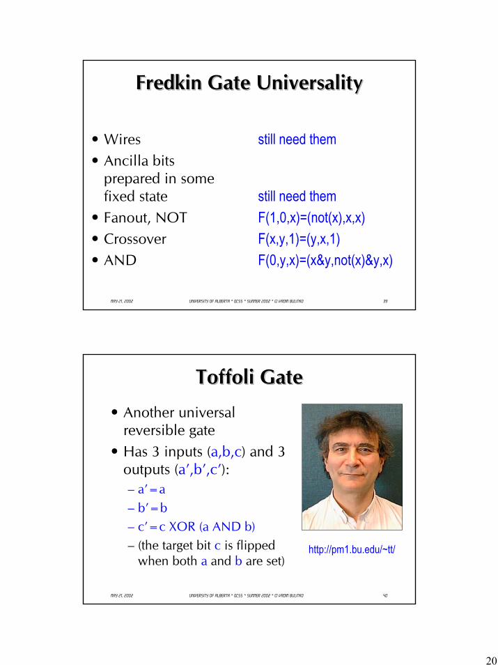
20
May 21, 2002 University of Alberta * QCSS * Summer 2002 * © Vadim Bulitko 39
Fredkin Gate UniversalityFredkin Gate UniversalityFredkin Gate Universality
• Wires still need them• Ancilla bits
prepared in some fixed state still need them
• Fanout, NOT F(1,0,x)=(not(x),x,x)• Crossover F(x,y,1)=(y,x,1)• AND F(0,y,x)=(x&y,not(x)&y,x)
May 21, 2002 University of Alberta * QCSS * Summer 2002 * © Vadim Bulitko 40
Toffoli GateToffoli GateToffoli Gate
• Another universal reversible gate
• Has 3 inputs (a,b,c) and 3 outputs (a’,b’,c’):– a’=a– b’=b– c’=c XOR (a AND b)– (the target bit c is flipped
when both a and b are set)http://pm1.bu.edu/~tt/
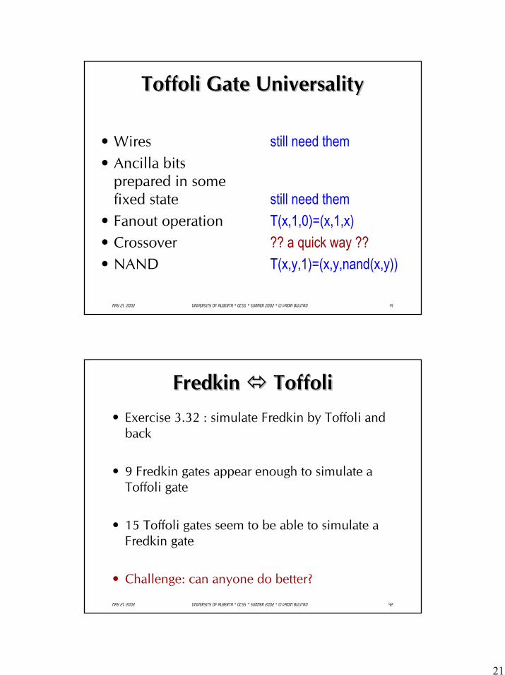
21
May 21, 2002 University of Alberta * QCSS * Summer 2002 * © Vadim Bulitko 41
Toffoli Gate UniversalityToffoli Gate UniversalityToffoli Gate Universality
• Wires still need them• Ancilla bits
prepared in some fixed state still need them
• Fanout operation T(x,1,0)=(x,1,x)• Crossover ?? a quick way ??• NAND T(x,y,1)=(x,y,nand(x,y))
May 21, 2002 University of Alberta * QCSS * Summer 2002 * © Vadim Bulitko 42
Fredkin ToffoliFredkin Fredkin ToffoliToffoli• Exercise 3.32 : simulate Fredkin by Toffoli and
back
• 9 Fredkin gates appear enough to simulate a Toffoli gate
• 15 Toffoli gates seem to be able to simulate a Fredkin gate
• Challenge: can anyone do better?
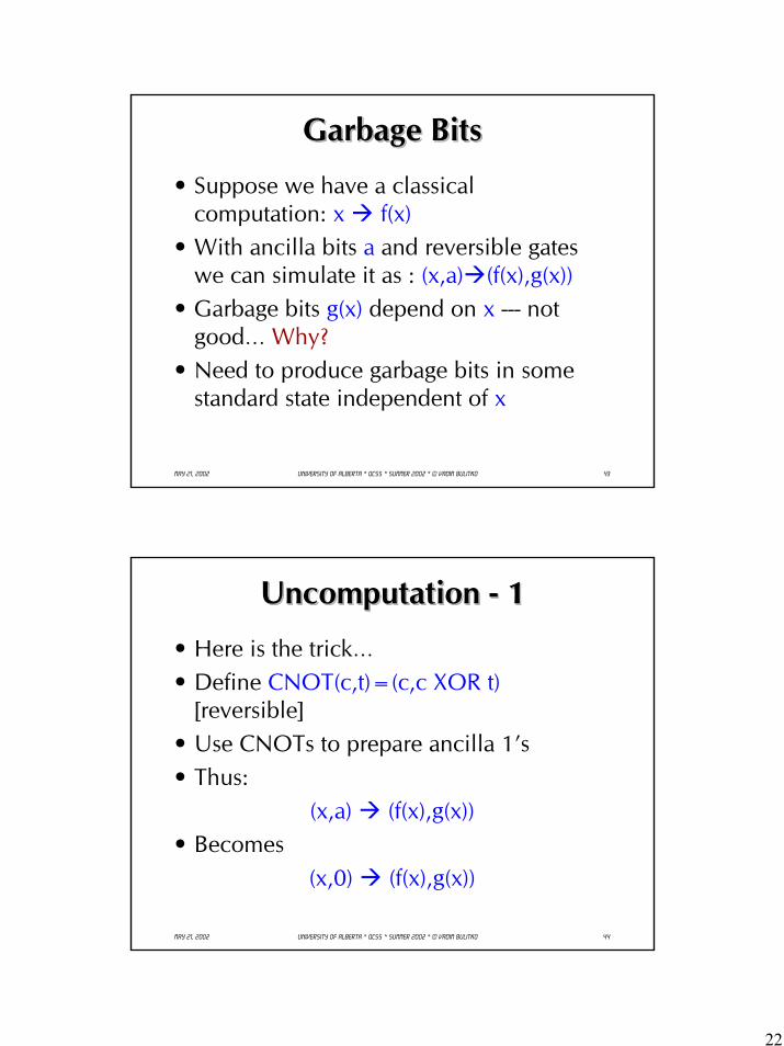
22
May 21, 2002 University of Alberta * QCSS * Summer 2002 * © Vadim Bulitko 43
Garbage BitsGarbage BitsGarbage Bits
• Suppose we have a classical computation: x f(x)
• With ancilla bits a and reversible gates we can simulate it as : (x,a) (f(x),g(x))
• Garbage bits g(x) depend on x --- not good… Why?
• Need to produce garbage bits in some standard state independent of x
May 21, 2002 University of Alberta * QCSS * Summer 2002 * © Vadim Bulitko 44
Uncomputation - 1Uncomputation Uncomputation -- 11
• Here is the trick…• Define CNOT(c,t)=(c,c XOR t)
[reversible]• Use CNOTs to prepare ancilla 1’s• Thus:
(x,a) (f(x),g(x))• Becomes
(x,0) (f(x),g(x))
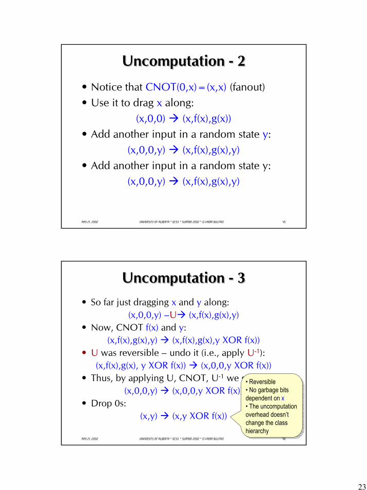
23
May 21, 2002 University of Alberta * QCSS * Summer 2002 * © Vadim Bulitko 45
Uncomputation - 2Uncomputation Uncomputation -- 22
• Notice that CNOT(0,x)=(x,x) (fanout)• Use it to drag x along:
(x,0,0) (x,f(x),g(x))• Add another input in a random state y:
(x,0,0,y) (x,f(x),g(x),y)• Add another input in a random state y:
(x,0,0,y) (x,f(x),g(x),y)
May 21, 2002 University of Alberta * QCSS * Summer 2002 * © Vadim Bulitko 46
Uncomputation - 3Uncomputation Uncomputation -- 33• So far just dragging x and y along:
(x,0,0,y) –U (x,f(x),g(x),y)• Now, CNOT f(x) and y:
(x,f(x),g(x),y) (x,f(x),g(x),y XOR f(x))• U was reversible – undo it (i.e., apply U-1):
(x,f(x),g(x), y XOR f(x)) (x,0,0,y XOR f(x))• Thus, by applying U, CNOT, U-1 we get:
(x,0,0,y) (x,0,0,y XOR f(x))• Drop 0s:
(x,y) (x,y XOR f(x))
• Reversible• No garbage bits dependent on x• The uncomputation overhead doesn’t change the class hierarchy
• Reversible• No garbage bits dependent on x• The uncomputation overhead doesn’t change the class hierarchy
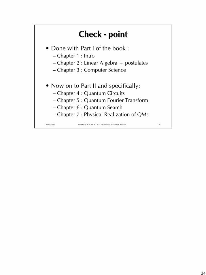
24
May 21, 2002 University of Alberta * QCSS * Summer 2002 * © Vadim Bulitko 47
Check - pointCheck Check -- pointpoint
• Done with Part I of the book : – Chapter 1 : Intro– Chapter 2 : Linear Algebra + postulates– Chapter 3 : Computer Science
• Now on to Part II and specifically:– Chapter 4 : Quantum Circuits– Chapter 5 : Quantum Fourier Transform– Chapter 6 : Quantum Search– Chapter 7 : Physical Realization of QMs
1
Chapter 4
QUANTUM CIRCUITS
Part ILecture 7
Vahid RezaniaMay-June 2002
Motivation• Quantum circuit model :
fundamental model for quantumcomputing
• Universal Gates:any quantum computation can be expressed by these gates
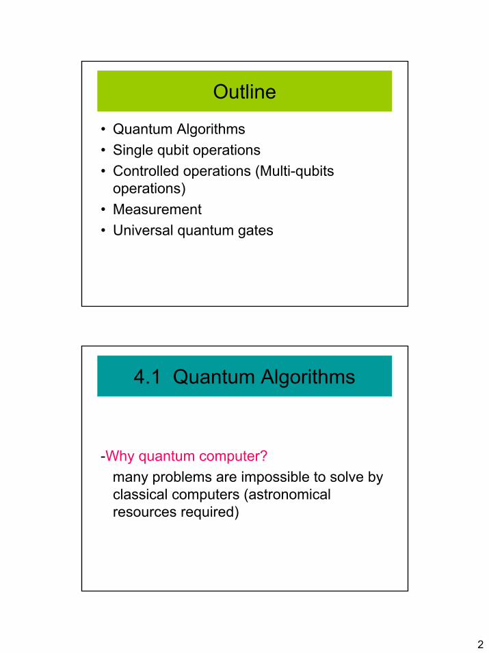
2
Outline
• Quantum Algorithms• Single qubit operations• Controlled operations (Multi-qubits
operations)• Measurement• Universal quantum gates
4.1 Quantum Algorithms
-Why quantum computer? many problems are impossible to solve by classical computers (astronomical resources required)
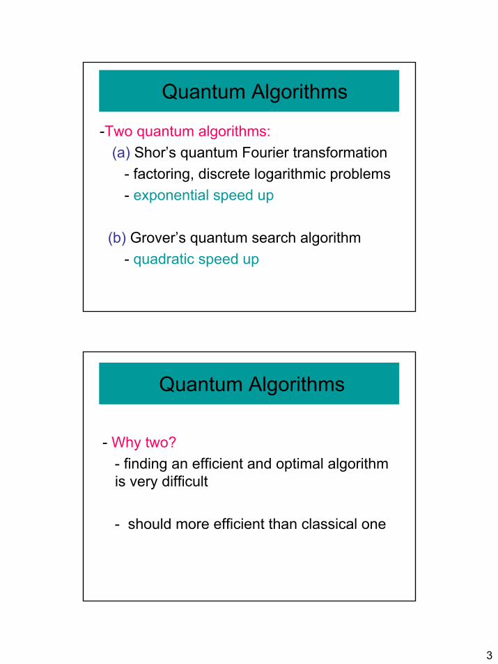
3
-Two quantum algorithms:(a) Shor’s quantum Fourier transformation
- factoring, discrete logarithmic problems- exponential speed up
(b) Grover’s quantum search algorithm - quadratic speed up
Quantum Algorithms
- Why two?- finding an efficient and optimal algorithm is very difficult
- should more efficient than classical one
Quantum Algorithms
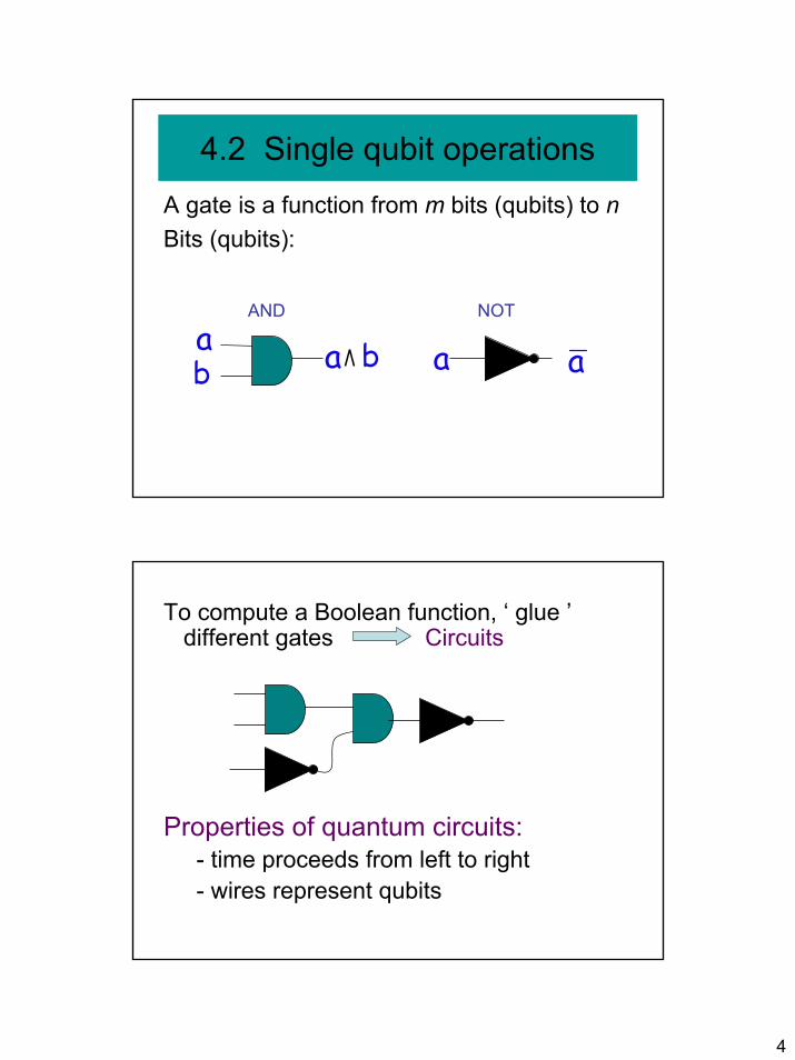
4
A gate is a function from m bits (qubits) to n Bits (qubits):
4.2 Single qubit operations
ab a b
AND
a aNOT
To compute a Boolean function, ‘ glue ’ different gates Circuits
Properties of quantum circuits:- time proceeds from left to right- wires represent qubits
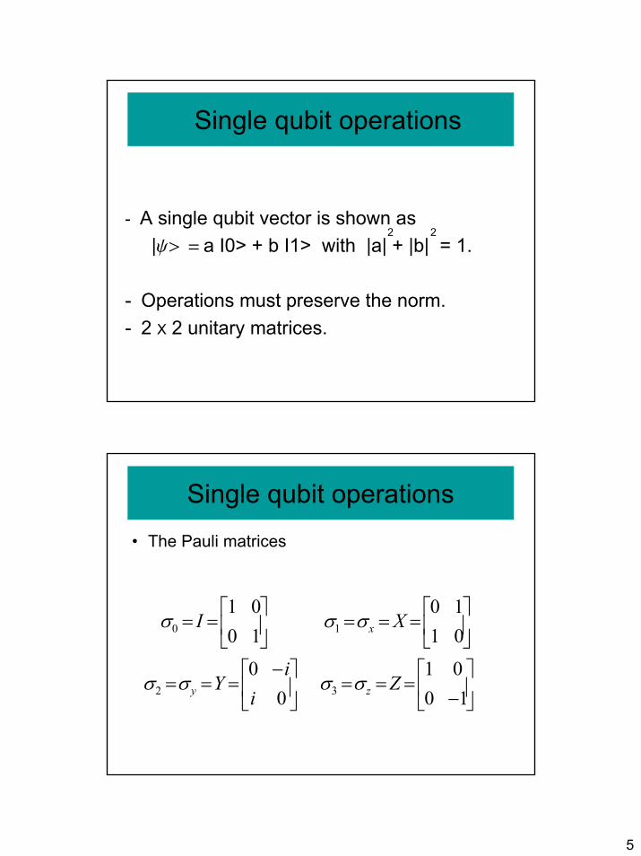
5
- A single qubit vector is shown as |y> = a I0> + b I1> with |a| + |b| = 1.
- Operations must preserve the norm. - 2 X 2 unitary matrices.
2 2
Single qubit operations
• The Pauli matrices
−
===
−===
===
==
1001
0
0
0110
1001
32
10
Zi
iY
XI
zy
x
σσσσ
σσσ
Single qubit operations
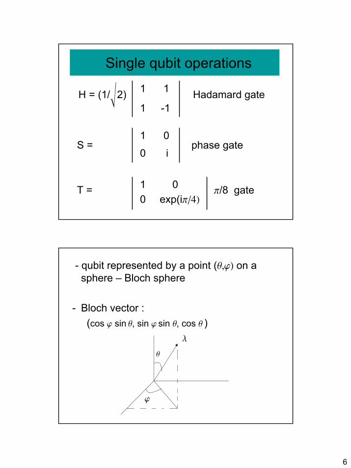
6
H = (1//2) Hadamard gate
S = phase gate
T = p/8 gate
-11
11
i001
exp(ip/4)001
Single qubit operations
- qubit represented by a point (q,j) on a sphere – Bloch sphere
- Bloch vector :(cos j sin q, sin j sin q, cos q )
l
q
j
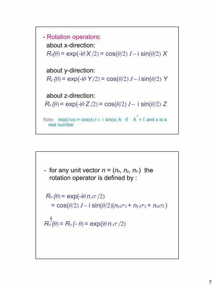
7
- Rotation operators: about x-direction: Rx(q) = exp(-iq X /2) = cos(q/2) I - i sin(q/2) X
about y-direction:Ry (q) = exp(-iq Y /2) = cos(q/2) I - i sin(q/2) Y
about z-direction:Rz (q) = exp(-iq Z /2) = cos(q/2) I - i sin(q/2) Z
Note: exp(iAx) = cos(x) I + i sin(x) A if A = I and x is a real number
2
- for any unit vector n = (nx, ny, nz ) the rotation operator is defined by :
Rn (q) = exp(-iq n.s /2)
= cos(q/2) I - i sin(q/2)(nxs x + ny s y + nzsz )
Rn (q) = Rn (- q) = exp(iq n.s /2)
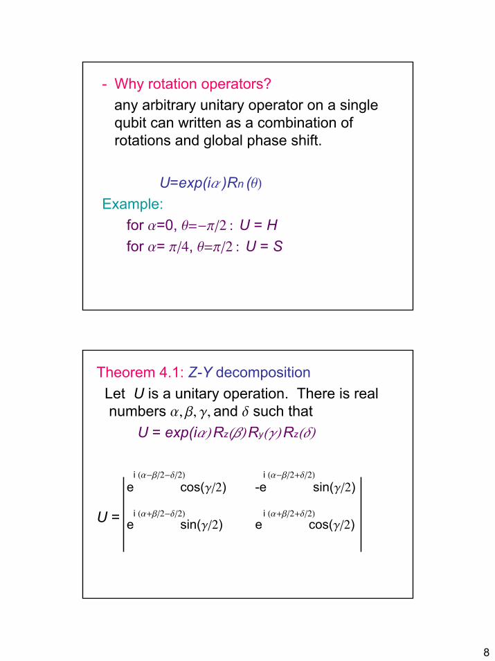
8
- Why rotation operators?any arbitrary unitary operator on a single qubit can written as a combination of rotations and global phase shift.
U=exp(ia )Rn (q)
Example:for a=0, q=-p/2 : U = Hfor a= p/4, q=p/2 : U = S
Theorem 4.1: Z-Y decompositionLet U is a unitary operation. There is real numbers a, b, g, and d such that
U = exp(ia) Rz(b) Ry(g) Rz(d)
U = e cos(g/2)e sin(g/2)
-e sin(g/2)e cos(g/2)i (a-b/2-d/2) i (a-b/2+d/2)
i (a+b/2-d/2) i (a+b/2+d/2)
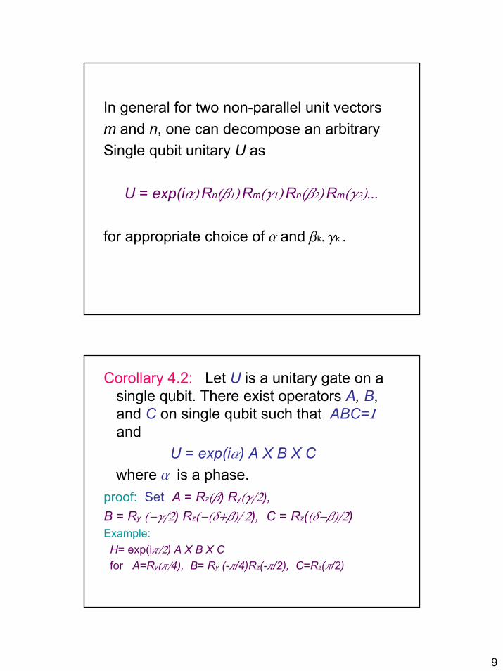
9
In general for two non-parallel unit vectors m and n, one can decompose an arbitrary Single qubit unitary U as
U = exp(ia) Rn(b1) Rm(g1) Rn(b2) Rm(g2)...
for appropriate choice of a and bk, gk .
Corollary 4.2: Let U is a unitary gate on a single qubit. There exist operators A, B, and C on single qubit such that ABC=Iand
U = exp(ia) A X B X Cwhere a is a phase.
proof: Set A = Rz(b) Ry(g/2), B = Ry (-g/2) Rz(-(d+b)/ 2), C = Rz((d-b)/2)Example:
H= exp(ip/2) A X B X Cfor A=Ry(p/4), B= Ry (-p/4)Rz(-p/2), C=Rz(p/2)
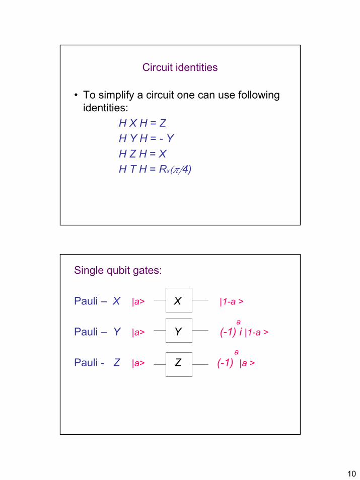
10
Circuit identities
• To simplify a circuit one can use following identities:
H X H = ZH Y H = - YH Z H = XH T H = Rx(p/4)
Single qubit gates:
Pauli – X |a> X |1-a >
Pauli – Y |a> Y (-1) i |1-a >
Pauli - Z |a> Z (-1) |a > a
a
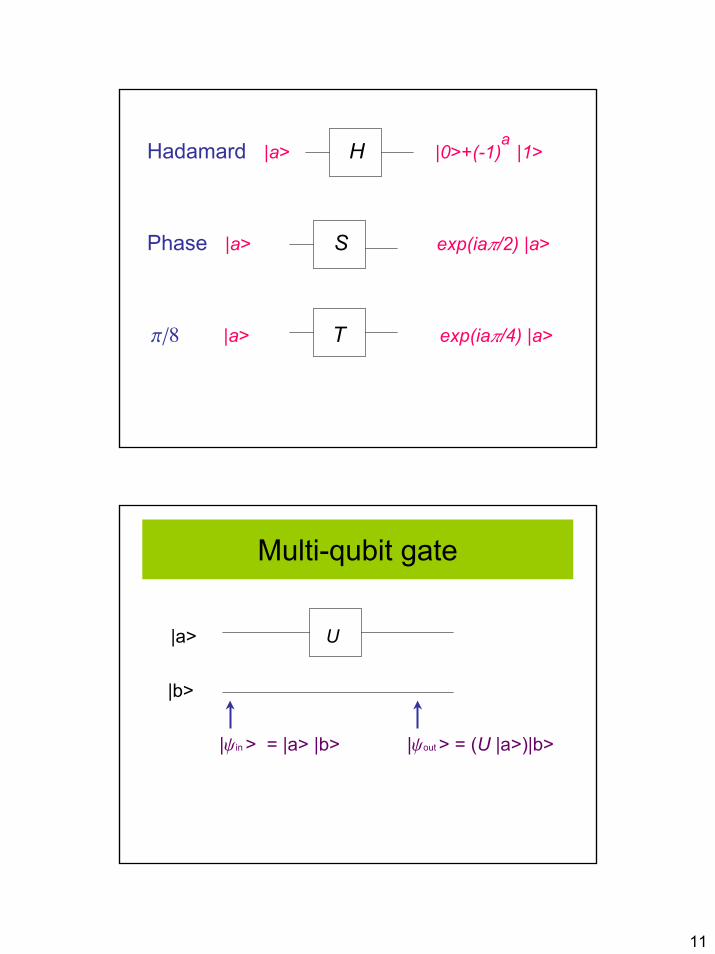
11
Hadamard |a> H |0>+(-1) |1>
Phase |a> S exp(iap/2) |a>
p/8 |a> T exp(iap/4) |a>
a
Multi-qubit gate
|a> U
|b>
|yin > = |a> |b> |yout > = (U |a>)|b>
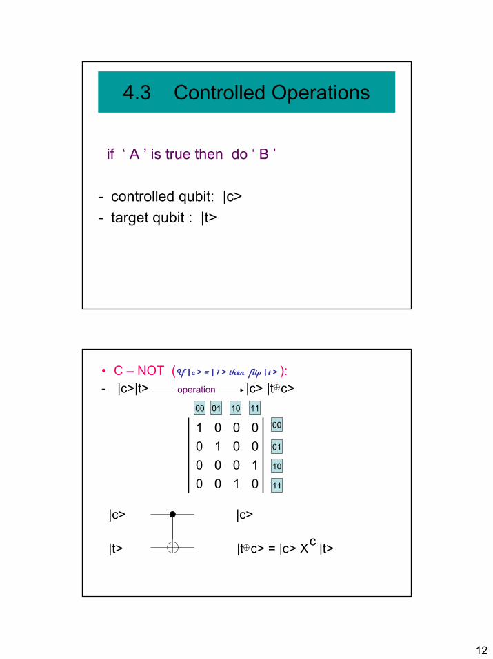
12
4.3 Controlled Operations
if ‘ A ’ is true then do ‘ B ’
- controlled qubit: |c>- target qubit : |t>
• C – NOT (If |c > = |1 > then flip |t > ):- |c>|t> operation |c> |t c>
|c> |c>
|t> |t c> = |c> X |t>
010010000010 00 01
c
00 01 10 11
00
01
10
11
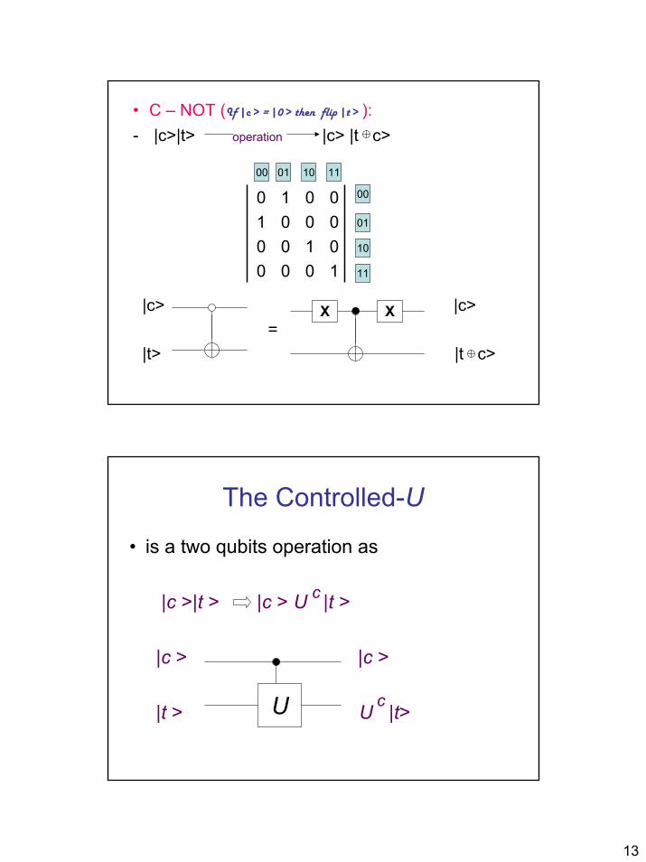
13
• C – NOT (If |c > = |0 > then flip |t > ):- |c>|t> operation |c> |t c>
|c> |c>=
|t> |t c>
100001000001 00 10
X X
00 01 10 11
00
01
10
11
The Controlled-U
• is a two qubits operation as
|c >|t > |c > U |t >
|c > |c >
|t > U |t>U
c
c
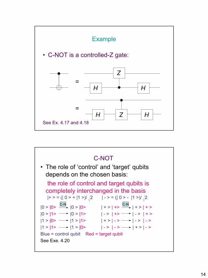
14
Example
• C-NOT is a controlled-Z gate:
=
=
See Ex. 4.17 and 4.18
HH Z
HH
Z
C-NOT• The role of ‘control’ and ‘target’ qubits
depends on the chosen basis: the role of control and target qubits is completely interchanged in the basis |+ > = (| 0 > + |1 >)/ /2 | - > = (| 0 > - |1 >)/ /2
|0 > |0> |0 > |0> | + > | +> | + > | + >|0 > |1> |0 > |1> | - > | +> | - > | + >|1 > |0> |1 > |1> | + > | - > | - > | - >|1 > |1> |1 > |0> | - > | - > | + > | - >Blue = control qubit Red = target qubitSee Exe. 4.20
C-N C-N
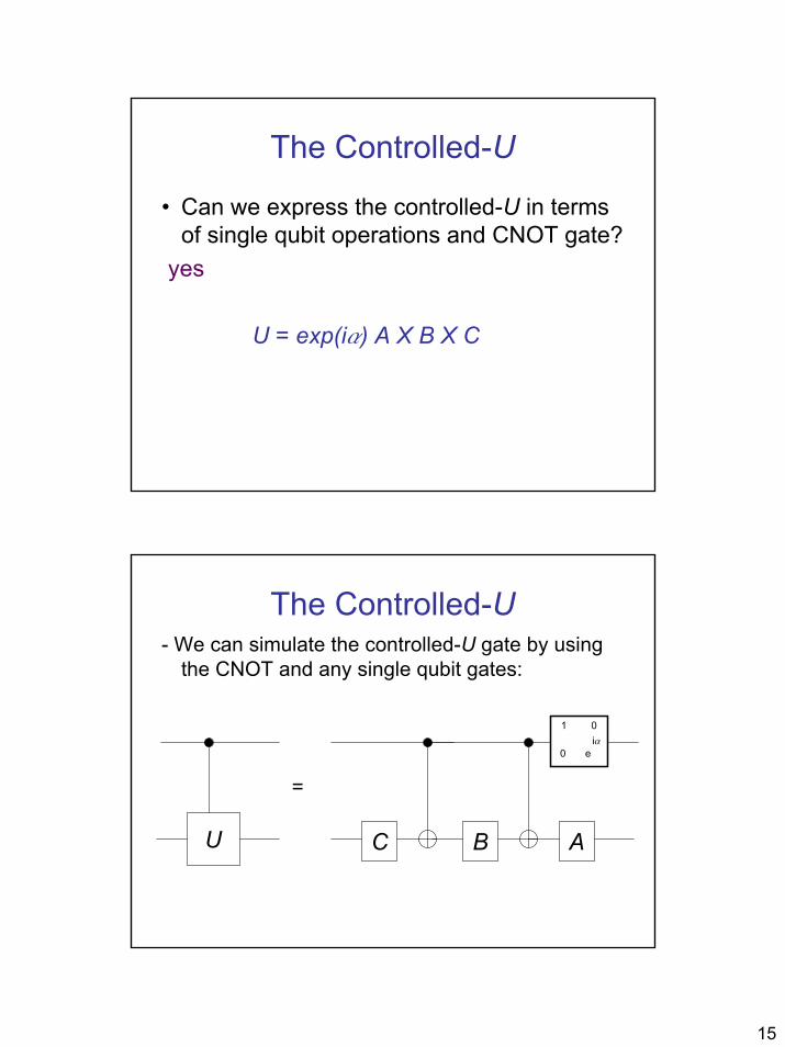
15
The Controlled-U
• Can we express the controlled-U in terms of single qubit operations and CNOT gate?
yes
U = exp(ia) A X B X C
The Controlled-U- We can simulate the controlled-U gate by using
the CNOT and any single qubit gates:
=
U C B A
e0
01ia

16
The Controlled-UIn general for n+k qubits and U is a k qubit
unitary operator : C (U)|x1x2..xn>|y> =|x1x2…xn>U |y>
n=4, k=3 U
x1x2…xnn
C (U):we can express C (U) by using any unitary
operator V such that V =U
=
U V V V
2
2
2
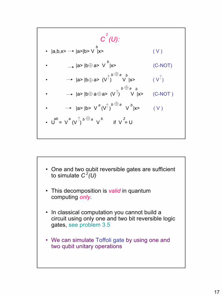
17
C (U):
• |a,b,x> |a>|b> V |x> ( V )
• |a> |b a> V |x> (C-NOT)
• |a> |b a> (V ) V |x> ( V )
• |a> |b a a> (V ) V |x> (C-NOT )
• |a> |b> V (V ) V |x> ( V )
• U = V (V ) V if V = U
2
b
b
bb a
b
b a
a b a b
b a
baab 2
• One and two qubit reversible gates are sufficient to simulate C (U)
• This decomposition is valid in quantum computing only.
• In classical computation you cannot build a circuit using only one and two bit reversible logic gates, see problem 3.5
• We can simulate Toffoli gate by using one and two qubit unitary operations
2
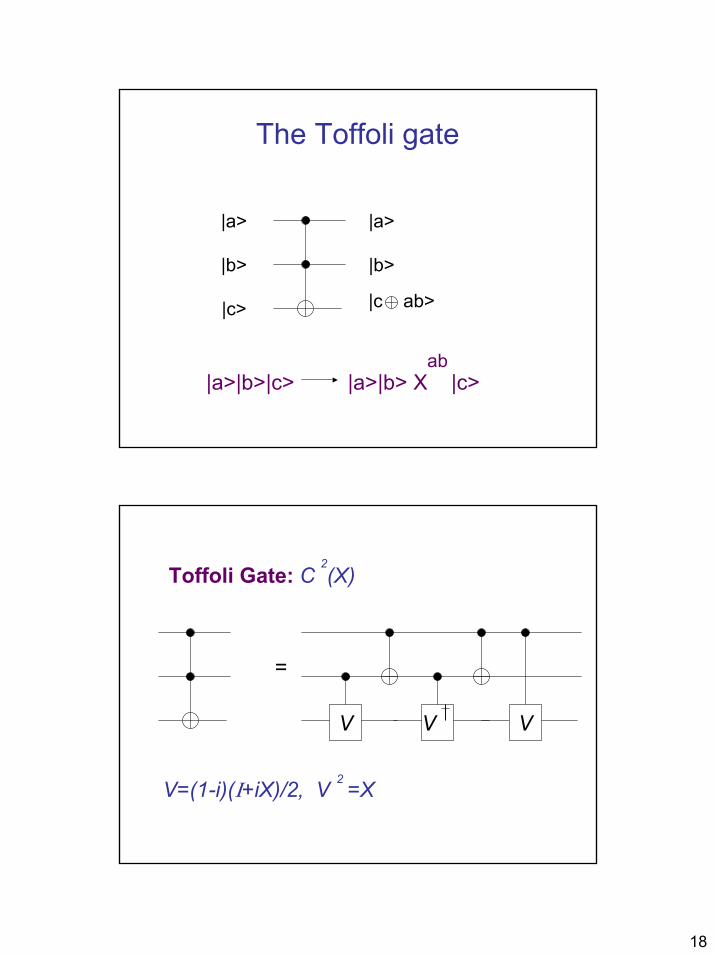
18
The Toffoli gate
|a>|b>|c> |a>|b> X |c>
|a>
|b>
|c>
|a>
|b>
|c ab>
ab
Toffoli Gate: C (X)
=
V=(1-i)(I+iX)/2, V =X
V V V
2
2
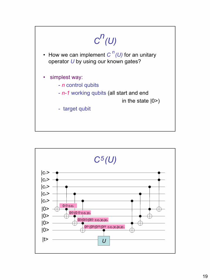
19
C (U)• How we can implement C (U) for an unitary
operator U by using our known gates?
• simplest way: - n control qubits - n-1 working qubits (all start and end
in the state |0>)- target qubit
n
n
C (U)5
|c1>|c2>|c3>|c4>|c5>|0>|0>|0>|0>
|t> U
0 c1c2
0 (0 c1c2 )c3
0 (0 (0 c1c2 )c3)c4
0 (0 (0 (0 c1c2 )c3)c4)c 5
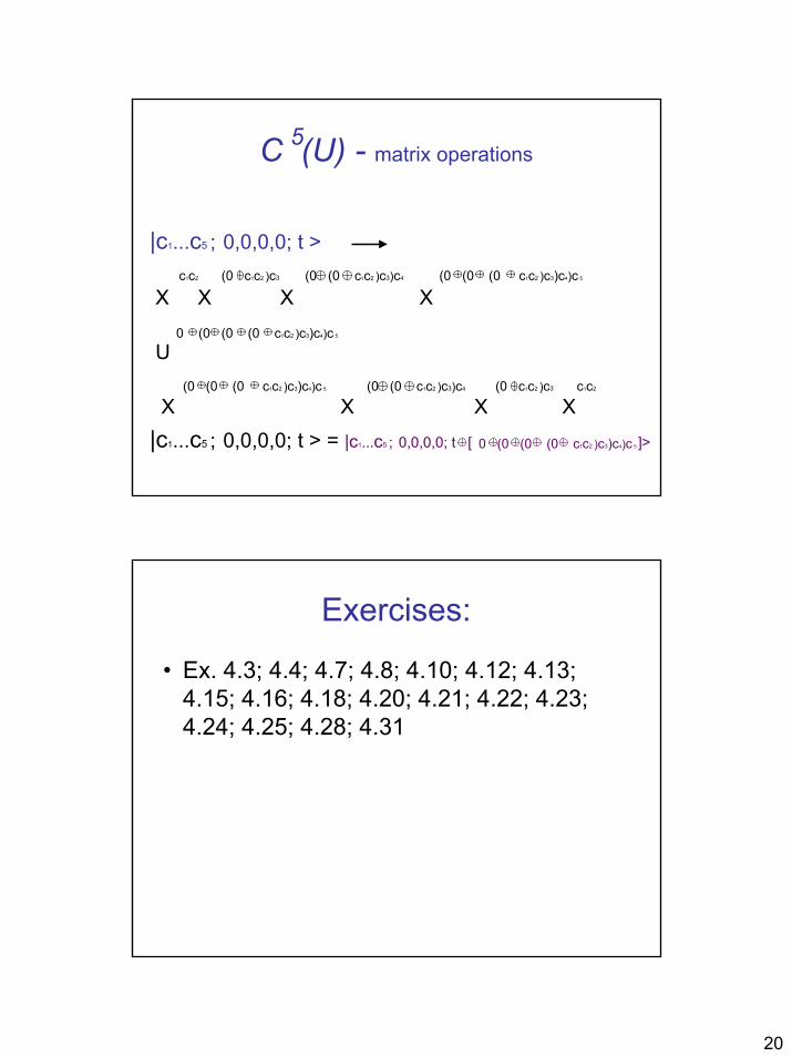
20
C (U) - matrix operations
|c1...c5 ; 0,0,0,0; t >
X X X X
U
X X X X|c1...c5 ; 0,0,0,0; t > = |c1...c5 ; 0,0,0,0; t [ ]>
5
c1c2
(0 c1c2 )c3 (0 (0 c1c2 )c3)c4 (0 (0 (0 c1c2 )c3)c4)c 5
0 (0 (0 (0 c1c2 )c3)c4)c 5
c1c2
(0 c1c2 )c3(0 (0 c1c2 )c3)c4(0 (0 (0 c1c2 )c3)c4)c 5
0 (0 (0 (0 c1c2 )c3)c4)c 5
Exercises:
• Ex. 4.3; 4.4; 4.7; 4.8; 4.10; 4.12; 4.13; 4.15; 4.16; 4.18; 4.20; 4.21; 4.22; 4.23; 4.24; 4.25; 4.28; 4.31
1
Chapter 4
QUANTUM CIRCUITS
Part IILecture 8
Vahid RezaniaMay-June 2002
Overview
• Deferred and implicit measurements
• Universality
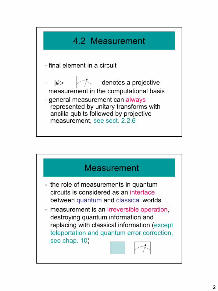
2
4.2 Measurement
- final element in a circuit
- |y> denotes a projectivemeasurement in the computational basis
- general measurement can alwaysrepresented by unitary transforms with ancilla qubits followed by projective measurement, see sect. 2.2.6
Measurement
- the role of measurements in quantum circuits is considered as an interfacebetween quantum and classical worlds
- measurement is an irreversible operation, destroying quantum information and replacing with classical information (except teleportation and quantum error correction, see chap. 10)
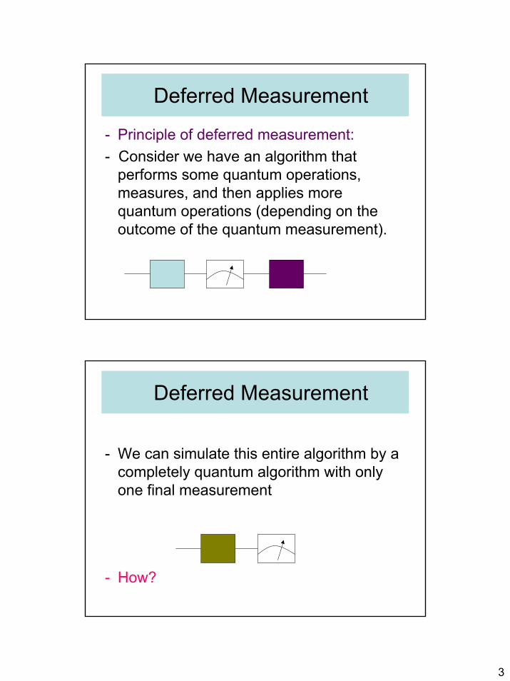
3
Deferred Measurement
- Principle of deferred measurement: - Consider we have an algorithm that
performs some quantum operations, measures, and then applies more quantum operations (depending on the outcome of the quantum measurement).
Deferred Measurement
- We can simulate this entire algorithm by a completely quantum algorithm with only one final measurement
- How?
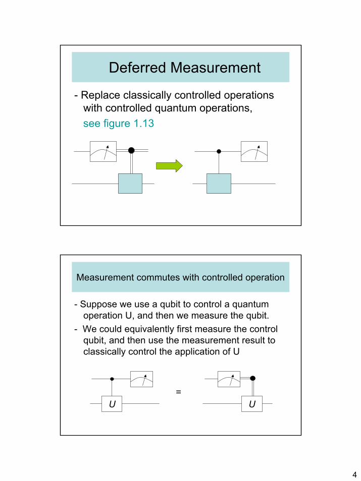
4
Deferred Measurement
- Replace classically controlled operations with controlled quantum operations, see figure 1.13
Measurement commutes with controlled operation
- Suppose we use a qubit to control a quantum operation U, and then we measure the qubit.
- We could equivalently first measure the control qubit, and then use the measurement result to classically control the application of U
=UU
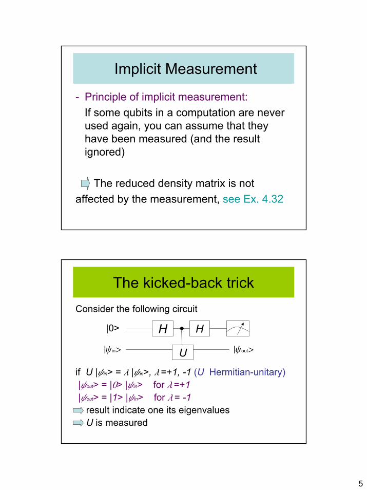
5
Implicit Measurement
- Principle of implicit measurement: If some qubits in a computation are never used again, you can assume that they have been measured (and the result ignored)
The reduced density matrix is not affected by the measurement, see Ex. 4.32
The kicked-back trickConsider the following circuit
if U |yin> = l |yin>, l =+1, -1 (U Hermitian-unitary)|yout> = |0> |yin> for l =+1|yout> = |1> |yin> for l = -1
result indicate one its eigenvaluesU is measured
H
U
H|0>
|yin> |yout>
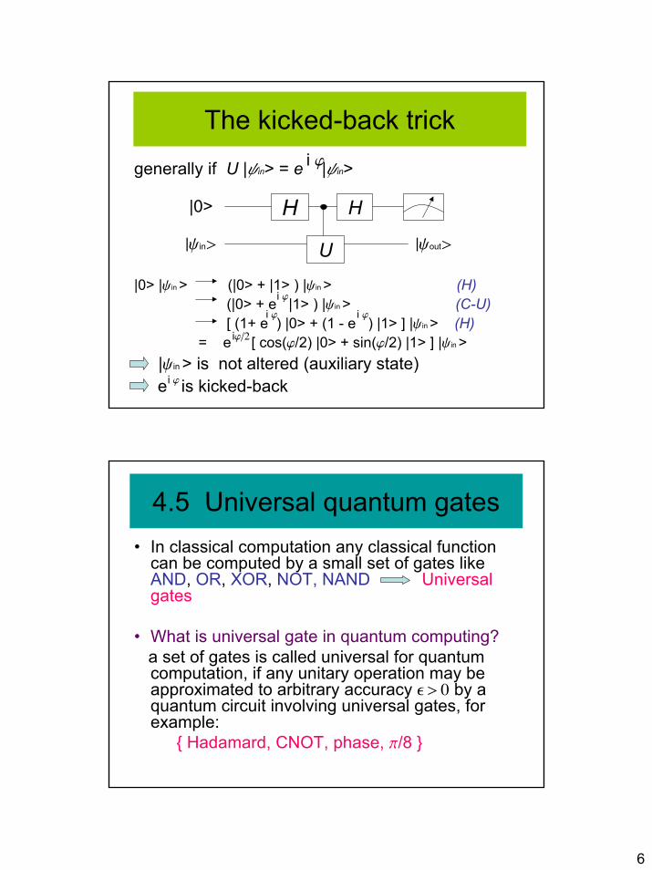
6
The kicked-back trickgenerally if U |yin> = e |yin>
|0> |yin > (|0> + |1> ) |yin > (H)(|0> + e |1> ) |yin > (C-U)[ (1+ e ) |0> + (1 - e ) |1> ] |yin > (H)
= e [ cos(j/2) |0> + sin(j/2) |1> ] |yin >|yin > is not altered (auxiliary state)e is kicked-back
i j
H
U
H|0>
|yin> |yout>
i ji j i j
ij/2
i j
4.5 Universal quantum gates• In classical computation any classical function
can be computed by a small set of gates like AND, OR, XOR, NOT, NAND Universal gates
• What is universal gate in quantum computing? a set of gates is called universal for quantum computation, if any unitary operation may be approximated to arbitrary accuracy e > 0 by a quantum circuit involving universal gates, for example:
Hadamard, CNOT, phase, p/8
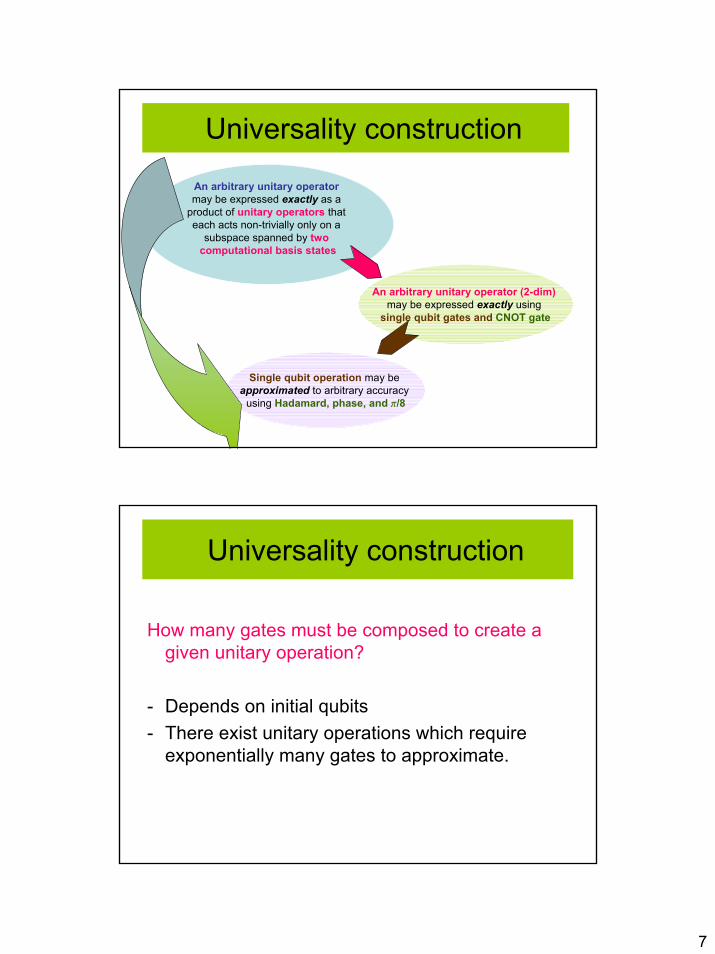
7
Universality construction
An arbitrary unitary operator may be expressed exactly as a
product of unitary operators that each acts non-trivially only on a
subspace spanned by two computational basis states
An arbitrary unitary operator (2-dim)may be expressed exactly using
single qubit gates and CNOT gate
Single qubit operation may be approximated to arbitrary accuracy
using Hadamard, phase, and p/8
Universality construction
How many gates must be composed to create a given unitary operation?
- Depends on initial qubits- There exist unitary operations which require
exponentially many gates to approximate.
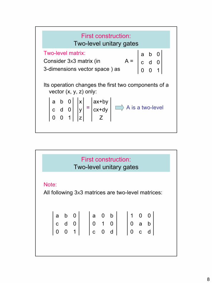
8
First construction:Two-level unitary gates
Two-level matrix:Consider 3X3 matrix (in A =3-dimensions vector space ) as
Its operation changes the first two components of a vector (x, y, z) only:
= A is a two-level
1000dc0ba
zyx
1000dc0ba
Zcx+dyax+by
First construction:Two-level unitary gates
Note:All following 3X3 matrices are two-level matrices:
1000dc0ba
d0c010b0a
dc0ba0001
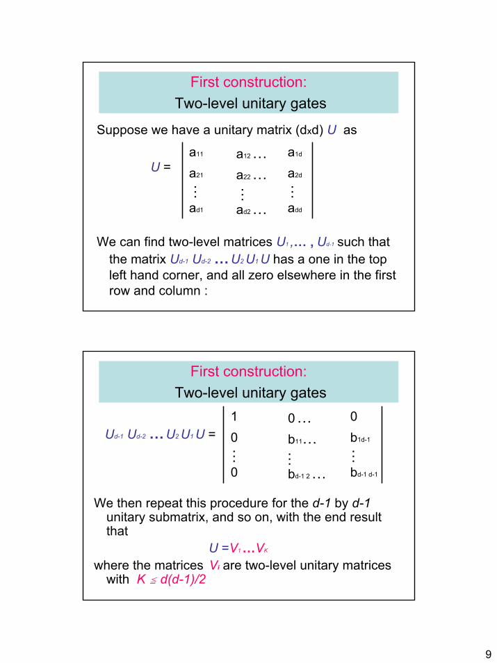
9
First construction:Two-level unitary gates
Suppose we have a unitary matrix (dxd) U as
U =
We can find two-level matrices U1 ,… , Ud-1 such that the matrix Ud-1 Ud-2 …U2 U1 U has a one in the top left hand corner, and all zero elsewhere in the first row and column :
addad2 …ad1
a2da22 …a21
a1da12 …a11
… … …
First construction:Two-level unitary gates
Ud-1 Ud-2 …U2 U1 U =
We then repeat this procedure for the d-1 by d-1 unitary submatrix, and so on, with the end result that
U =V1 …VK
where the matrices Vi are two-level unitary matrices with K c d(d-1)/2
bd-1 d-1bd-1 2 …0
b1d-1b11…000…1
… … …
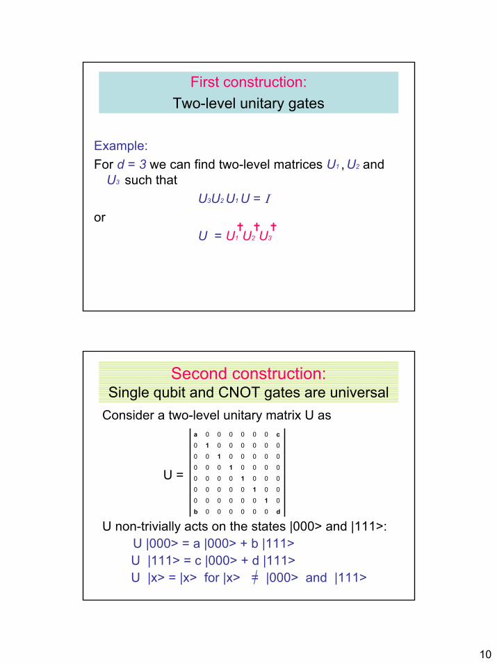
10
First construction:Two-level unitary gates
Example: For d = 3 we can find two-level matrices U1 , U2 and
U3 such thatU3U2 U1 U = I
orU = U1 U2 U3
Second construction:Single qubit and CNOT gates are universal
Consider a two-level unitary matrix U as
U =
U non-trivially acts on the states |000> and |111>: U |000> = a |000> + b |111>U |111> = c |000> + d |111>U |x> = |x> for |x> = |000> and |111>
d000000b010000000010000000010000000010000000010000000010c000000a
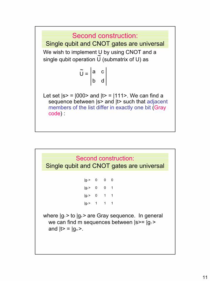
11
Second construction:Single qubit and CNOT gates are universal
We wish to implement U by using CNOT and a single qubit operation U (submatrix of U) as
U =
Let set |s> = |000> and |t> = |111>. We can find a sequence between |s> and |t> such that adjacent members of the list differ in exactly one bit (Gray code) :
dbca
~
~
Second construction:Single qubit and CNOT gates are universal
where |g1 > to |g4 > are Gray sequence. In general we can find m sequences between |s>= |g1 > and |t> = |gm >.
111|g4 >
110|g3 >
100|g2 >
000|g1 >
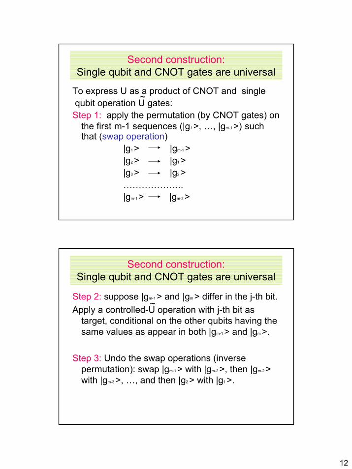
12
To express U as a product of CNOT and singlequbit operation U gates:
Step 1: apply the permutation (by CNOT gates) on the first m-1 sequences (|g1 >, …, |gm-1 >) such that (swap operation)
|g1 > |gm-1 > |g2 > |g1 > |g3 > |g2 > ………………..|gm-1 > |gm-2 >
Second construction:Single qubit and CNOT gates are universal
~
Step 2: suppose |gm-1 > and |gm > differ in the j-th bit. Apply a controlled-U operation with j-th bit as
target, conditional on the other qubits having the same values as appear in both |gm-1 > and |gm >.
Step 3: Undo the swap operations (inverse permutation): swap |gm-1 > with |gm-2 >, then |gm-2 > with |gm-3 >, …, and then |g2 > with |g1 >.
Second construction:Single qubit and CNOT gates are universal
~
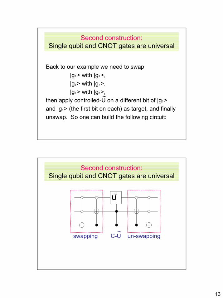
13
Back to our example we need to swap |g1 > with |g3 >, |g2 > with |g1 >, |g3 > with |g2 >,
then apply controlled-U on a different bit of |g3 > and |g4 > (the first bit on each) as target, and finally unswap. So one can build the following circuit:
Second construction:Single qubit and CNOT gates are universal
~
swapping C-U un-swapping
Second construction:Single qubit and CNOT gates are universal
U~
~
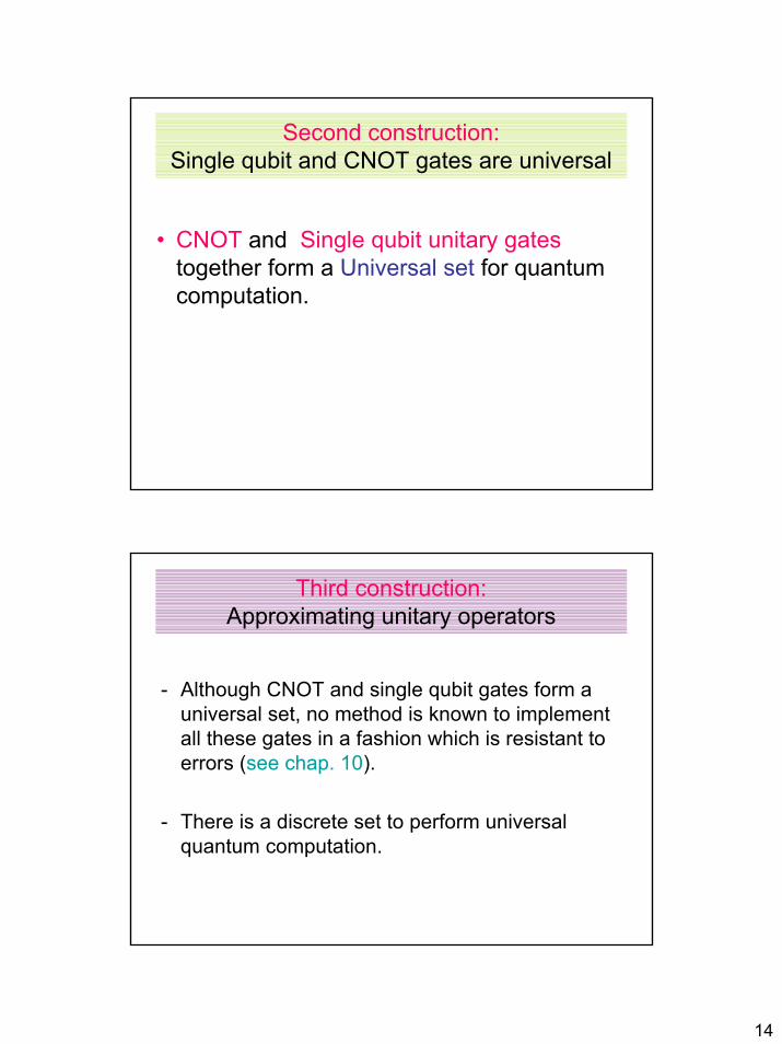
14
• CNOT and Single qubit unitary gates together form a Universal set for quantum computation.
Second construction:Single qubit and CNOT gates are universal
- Although CNOT and single qubit gates form a universal set, no method is known to implement all these gates in a fashion which is resistant to errors (see chap. 10).
- There is a discrete set to perform universal quantum computation.
Third construction:Approximating unitary operators
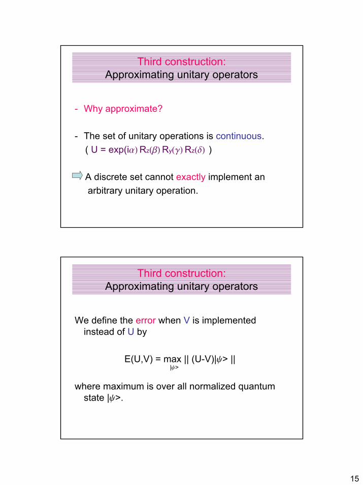
15
- Why approximate?
- The set of unitary operations is continuous.( U = exp(ia) Rz(b) Ry(g) Rz(d) )
A discrete set cannot exactly implement an arbitrary unitary operation.
Third construction:Approximating unitary operators
Third construction:Approximating unitary operators
We define the error when V is implemented instead of U by
E(U,V) = max || (U-V)|y> ||
where maximum is over all normalized quantum state |y>.
|y>
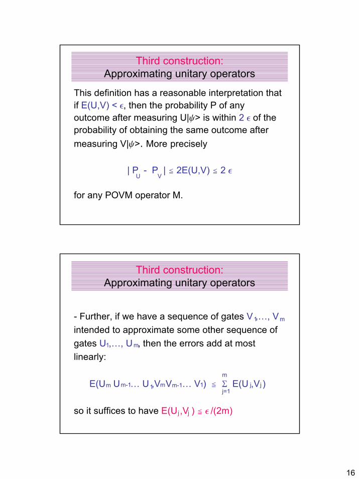
16
This definition has a reasonable interpretation that if E(U,V) < e, then the probability P of anyoutcome after measuring U|y> is within 2 e of theprobability of obtaining the same outcome aftermeasuring V|y>. More precisely
| P - P | c 2E(U,V) c 2 e
for any POVM operator M.
Third construction:Approximating unitary operators
U V
- Further, if we have a sequence of gates V ,…, Vintended to approximate some other sequence of gates U ,…, U , then the errors add at mostlinearly:
E(U U … U ,V V … V ) c S E(U ,V )
so it suffices to have E(U ,V ) c e /(2m)
Third construction:Approximating unitary operators
m1
1 m
m m-1 1 m m-1 1 j jj=1
m
j j
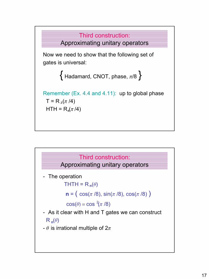
17
Now we need to show that the following set of gates is universal:
Hadamard, CNOT, phase, p/8 Remember (Ex. 4.4 and 4.11): up to global phase
T = R (p /4) HTH = R (p /4)
Third construction:Approximating unitary operators
x
z
- The operation THTH = R (q)
n = ( cos(p /8), sin(p /8), cos(p /8) ) cos(q) = cos (p /8)
- As it clear with H and T gates we can construct R (q)
- q is irrational multiple of 2p
Third construction:Approximating unitary operators
n
2
n
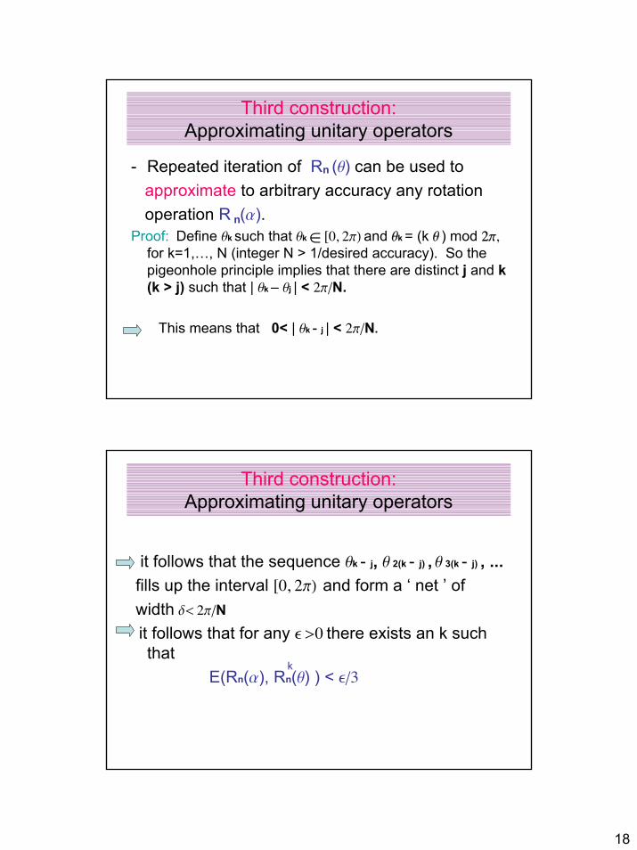
18
- Repeated iteration of R (q) can be used to approximate to arbitrary accuracy any rotation operation R (a).
Proof: Define qk such that qk [0, 2p) and qk = (k q ) mod 2p, for k=1,…, N (integer N > 1/desired accuracy). So the pigeonhole principle implies that there are distinct j and k(k > j) such that | qk – qj | < 2p/N.
This means that 0< | qk - j | < 2p/N.
Third construction:Approximating unitary operators
n
n
∈
it follows that the sequence qk - j, q 2(k - j) , q 3(k - j) , ...fills up the interval [0, 2p) and form a ‘ net ’ of width d< 2p/Nit follows that for any e >0 there exists an k such that
E(Rn(a), Rn(q) ) < e/3
Third construction:Approximating unitary operators
k
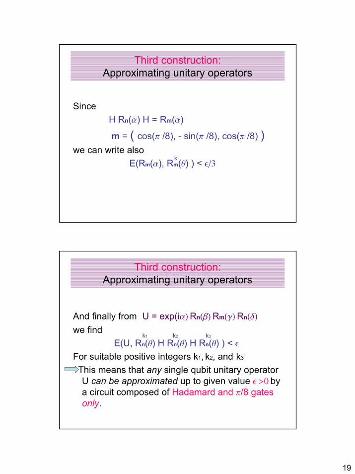
19
Since H Rn(a) H = Rm(a)
m = ( cos(p /8), - sin(p /8), cos(p /8) ) we can write also
E(Rm(a), Rm(q) ) < e/3
Third construction:Approximating unitary operators
k
And finally from U = exp(ia) Rn(b) Rm(g) Rn(d)
we find E(U, Rn(q) H Rn(q) H Rn(q) ) < e
For suitable positive integers k1, k2, and k3
This means that any single qubit unitary operator U can be approximated up to given value e >0 by a circuit composed of Hadamard and p/8 gates only.
Third construction:Approximating unitary operators
k1 k2 k3
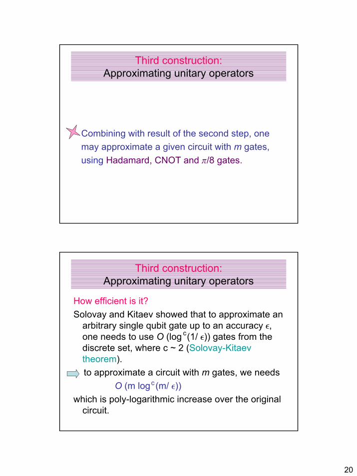
20
Combining with result of the second step, onemay approximate a given circuit with m gates,using Hadamard, CNOT and p/8 gates.
Third construction:Approximating unitary operators
How efficient is it? Solovay and Kitaev showed that to approximate an
arbitrary single qubit gate up to an accuracy e, one needs to use O (log (1/ e)) gates from the discrete set, where c ~ 2 (Solovay-Kitaevtheorem). to approximate a circuit with m gates, we needs
O (m log (m/ e))which is poly-logarithmic increase over the original
circuit.
Third construction:Approximating unitary operators
c
c
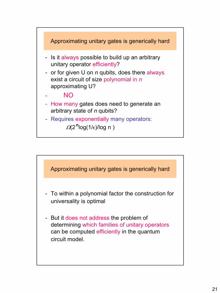
21
- Is it always possible to build up an arbitrary unitary operator efficiently?
- or for given U on n qubits, does there alwaysexist a circuit of size polynomial in napproximating U?
- NO- How many gates does need to generate an
arbitrary state of n qubits?- Requires exponentially many operators:
W(2 log(1/e)/log n )
Approximating unitary gates is generically hard
n
- To within a polynomial factor the construction for universality is optimal
- But it does not address the problem of determining which families of unitary operatorscan be computed efficiently in the quantum circuit model.
Approximating unitary gates is generically hard
22
• Ex. 4.32; 4.34; 4.35; 4.37; 4.38; 4.39; 4.40; 4.41; 4.44
Exercises
1
Chapter 4
QUANTUM CIRCUITS
Part IIILecture 9
Vahid RezaniaMay-June 2002
Overview
• Quantum computational complexity
• Simulation of quantum circuit
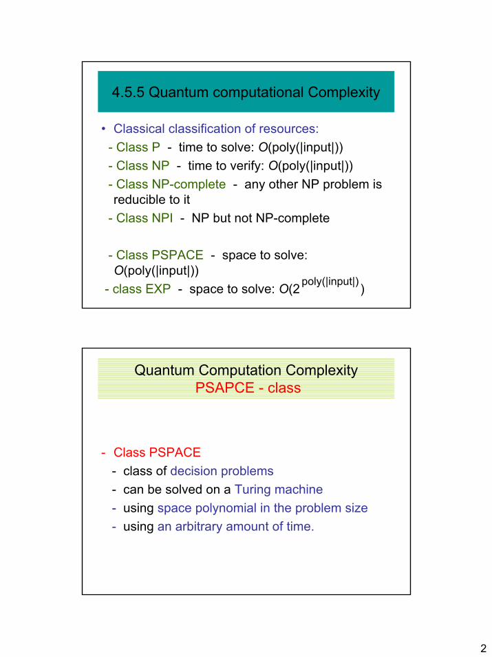
2
4.5.5 Quantum computational Complexity
• Classical classification of resources:- Class P - time to solve: O(poly(|input|))- Class NP - time to verify: O(poly(|input|))- Class NP-complete - any other NP problem is reducible to it
- Class NPI - NP but not NP-complete
- Class PSPACE - space to solve: O(poly(|input|))
- class EXP - space to solve: O(2 )poly(|input|)
Quantum Computation Complexity PSAPCE - class
- Class PSPACE - class of decision problems- can be solved on a Turing machine- using space polynomial in the problem size - using an arbitrary amount of time.
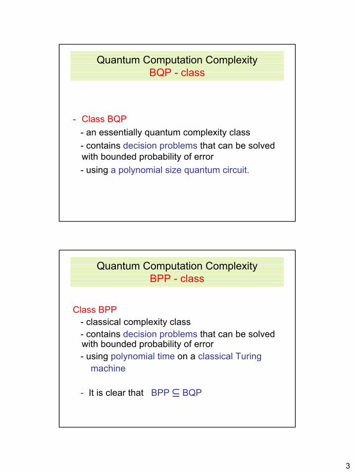
3
Quantum Computation Complexity BQP - class
- Class BQP - an essentially quantum complexity class - contains decision problems that can be solved with bounded probability of error - using a polynomial size quantum circuit.
Quantum Computation Complexity BPP - class
Class BPP - classical complexity class - contains decision problems that can be solved with bounded probability of error - using polynomial time on a classical Turing
machine
- It is clear that BPP BQP
UI
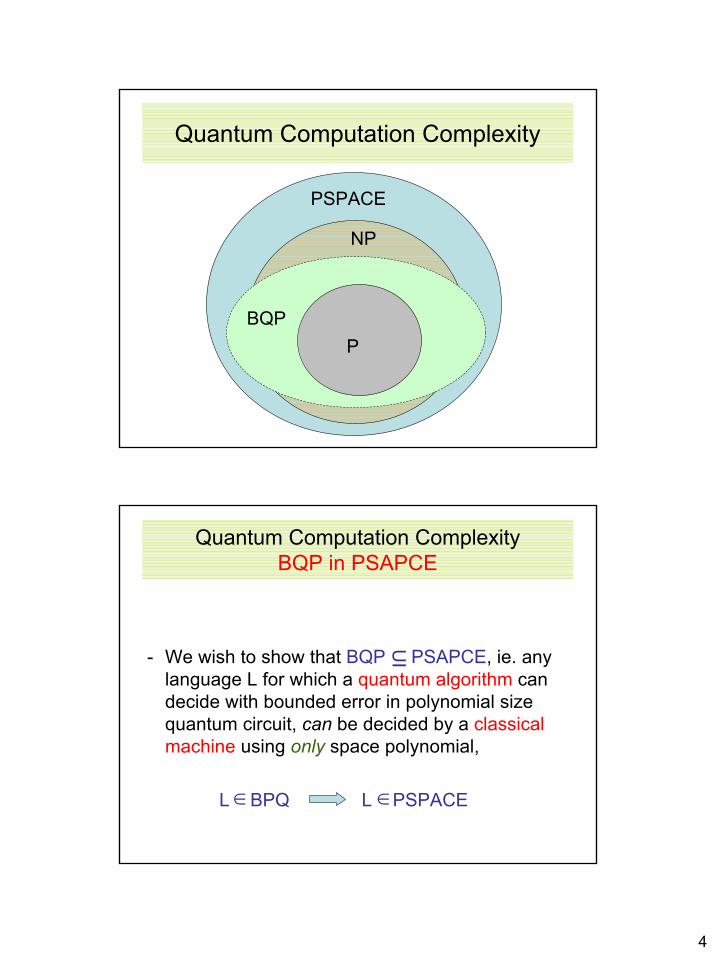
4
Quantum Computation Complexity
PBQP
NP
PSPACE
Quantum Computation Complexity BQP in PSAPCE
- We wish to show that BQP PSAPCE, ie. any language L for which a quantum algorithm can decide with bounded error in polynomial size quantum circuit, can be decided by a classical machine using only space polynomial,
L BPQ L PSPACE
UI
∈ ∈
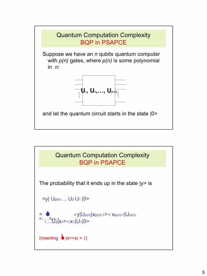
5
Quantum Computation Complexity BQP in PSAPCE
Suppose we have an n qubits quantum computer with p(n) gates, where p(n) is some polynomial in n:
and let the quantum circuit starts in the state |0>
U1, U2,…, Up (n)… …
Quantum Computation Complexity BQP in PSAPCE
The probability that it ends up in the state |y> is
<y| Up(n) … U2 U1 |0>
= <y|Up(n)|xp(n)-1>< xp(n)-1|Up(n)-
1…U2|x1><x1|U1|0>
(inserting |x><x| = I )
X1, …,Xp(n) -1
x
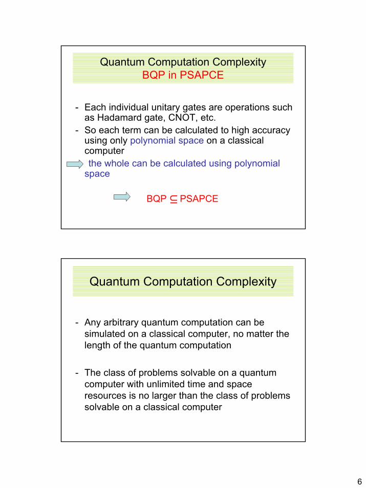
6
Quantum Computation Complexity BQP in PSAPCE
- Each individual unitary gates are operations such as Hadamard gate, CNOT, etc.
- So each term can be calculated to high accuracy using only polynomial space on a classical computerthe whole can be calculated using polynomial
space
BQP PSAPCEU
I
Quantum Computation Complexity
- Any arbitrary quantum computation can be simulated on a classical computer, no matter the length of the quantum computation
- The class of problems solvable on a quantum computer with unlimited time and space resources is no larger than the class of problems solvable on a classical computer
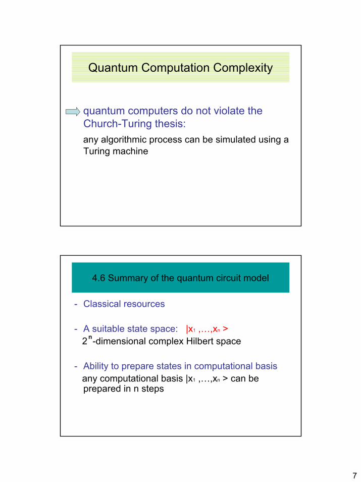
7
Quantum Computation Complexity
quantum computers do not violate the Church-Turing thesis:any algorithmic process can be simulated using a Turing machine
4.6 Summary of the quantum circuit model
- Classical resources
- A suitable state space: |x1 ,…,xn >2 -dimensional complex Hilbert space
- Ability to prepare states in computational basisany computational basis |x1 ,…,xn > can be prepared in n steps
n
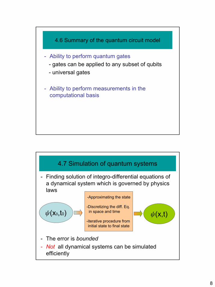
8
4.6 Summary of the quantum circuit model
- Ability to perform quantum gates- gates can be applied to any subset of qubits- universal gates
- Ability to perform measurements in the computational basis
4.7 Simulation of quantum systems
- Finding solution of integro-differential equations of a dynamical system which is governed by physics laws
- The error is bounded - Not all dynamical systems can be simulated
efficiently
y(x0,t0) y(x,t)
-Approximating the state
-Discretizing the diff. Eq. in space and time
-iterative procedure from initial state to final state
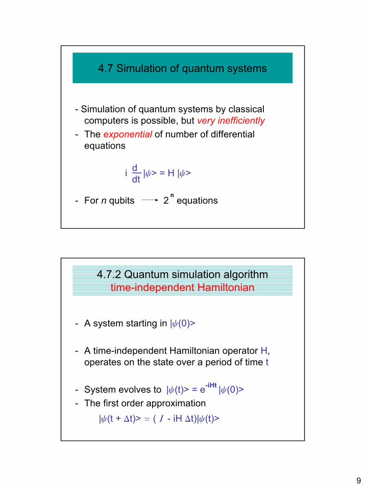
9
4.7 Simulation of quantum systems
- Simulation of quantum systems by classical computers is possible, but very inefficiently
- The exponential of number of differential equations
i |y> = H |y>
- For n qubits 2 equationsn
ddt__
4.7.2 Quantum simulation algorithmtime-independent Hamiltonian
- A system starting in |y(0)>
- A time-independent Hamiltonian operator H, operates on the state over a period of time t
- System evolves to |y(t)> = e |y(0)>- The first order approximation
|y(t + Dt)> > ( I - iH Dt)|y(t)>
-iHt
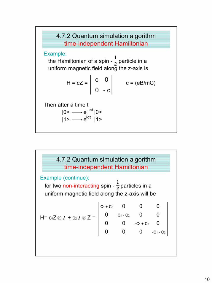
10
4.7.2 Quantum simulation algorithmtime-independent Hamiltonian
Example: the Hamiltonian of a spin - particle in auniform magnetic field along the z-axis is
H = cZ = c = (eB/mC)
Then after a time t |0> e |0> |1> e |1>
21
- c00c
-ict
ict
4.7.2 Quantum simulation algorithmtime-independent Hamiltonian
Example (continue): for two non-interacting spin - particles in auniform magnetic field along the z-axis will be
H= c1Z I + c2 I Z =
21
-c1 - c200 00-c1 + c20000 c1 - c20000c1 + c2
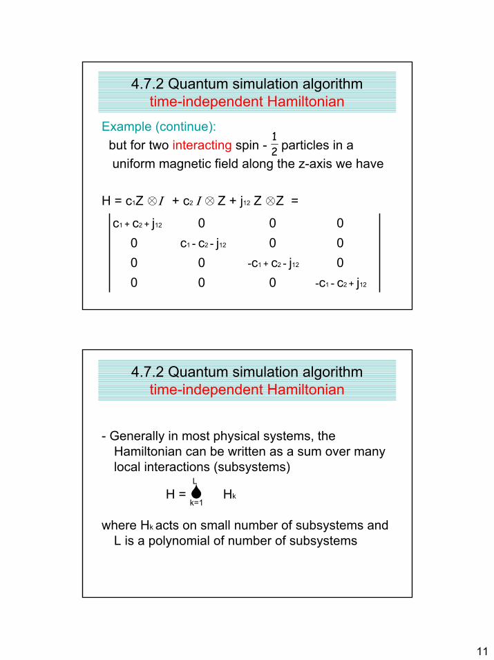
11
4.7.2 Quantum simulation algorithmtime-independent Hamiltonian
Example (continue): but for two interacting spin - particles in auniform magnetic field along the z-axis we have
H = c1Z I + c2 I Z + j12 Z Z =
21
-c1 - c2 + j1200 00-c1 + c2 - j120000 c1 - c2 - j120000c1 + c2 + j12
4.7.2 Quantum simulation algorithmtime-independent Hamiltonian
- Generally in most physical systems, the Hamiltonian can be written as a sum over many local interactions (subsystems)
H = Hk
where Hk acts on small number of subsystems and L is a polynomial of number of subsystems
k=1
L
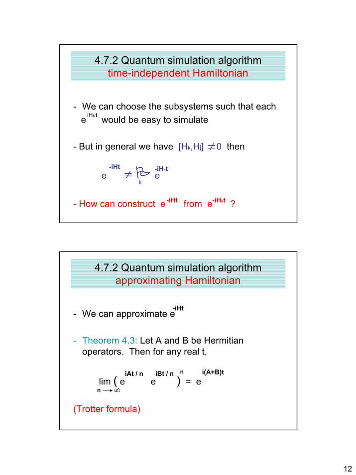
12
4.7.2 Quantum simulation algorithmtime-independent Hamiltonian
- We can choose the subsystems such that each e would be easy to simulate
- But in general we have [Hk,Hj] 0 then
e e
- How can construct e from e ?
iHk t
≠
≠-iHt -iHkt
k
-iHt -iHkt
4.7.2 Quantum simulation algorithmapproximating Hamiltonian
- We can approximate e
- Theorem 4.3: Let A and B be Hermitianoperators. Then for any real t,
lim ( e e ) = e
(Trotter formula)
-iHt
iAt / n iBt / n i(A+B)t
n ∞
n
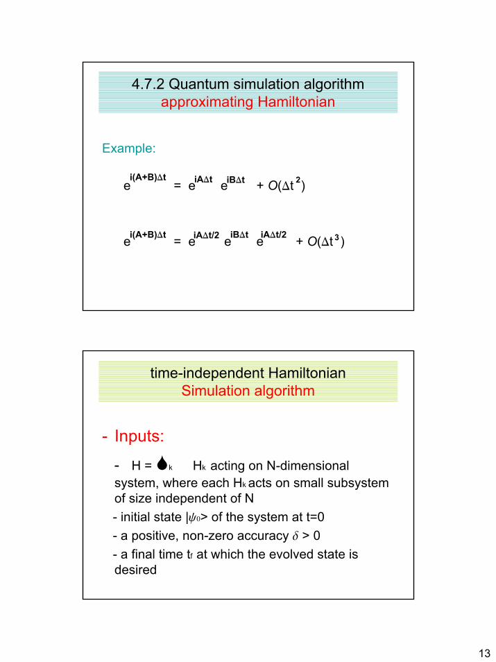
13
4.7.2 Quantum simulation algorithmapproximating Hamiltonian
Example:
e = e e + O(Dt )
e = e e e + O(Dt )
i(A+B)Dt
i(A+B)Dt
iADt iBDt
iADt/2 iBDt iADt/2
2
3
time-independent HamiltonianSimulation algorithm
- Inputs:
- H = k Hk acting on N-dimensional system, where each Hk acts on small subsystem of size independent of N- initial state |y0> of the system at t=0- a positive, non-zero accuracy d > 0- a final time tf at which the evolved state is desired
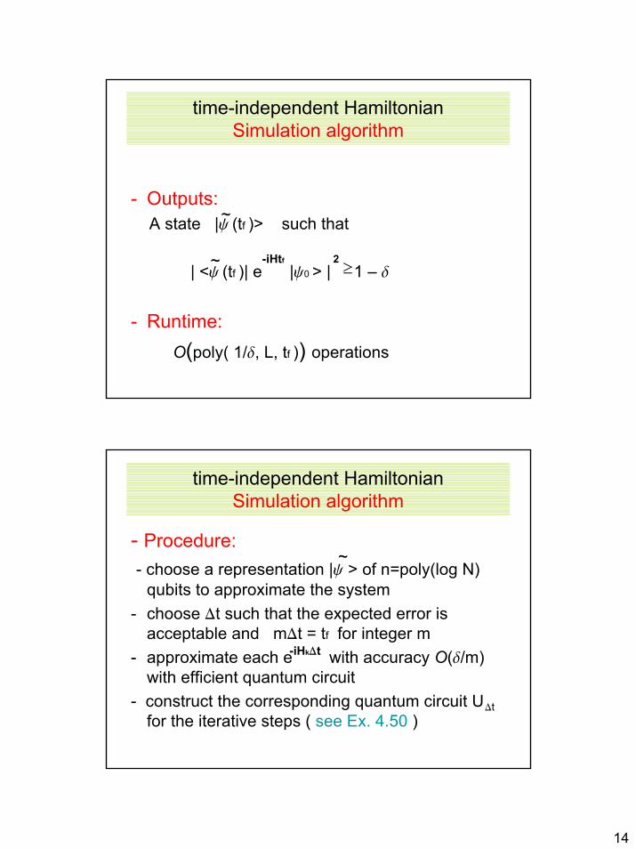
14
time-independent HamiltonianSimulation algorithm
- Outputs: A state |y (tf )> such that
| <y (tf )| e |y0 > | 1 – d
- Runtime: O(poly( 1/d, L, tf )) operations
~
~ -iHtf 2≥
time-independent HamiltonianSimulation algorithm
- Procedure: - choose a representation |y > of n=poly(log N)
qubits to approximate the system- choose Dt such that the expected error is
acceptable and mDt = tf for integer m- approximate each e with accuracy O(d/m)
with efficient quantum circuit- construct the corresponding quantum circuit U
for the iterative steps ( see Ex. 4.50 )
~
-iHkDt
Dt
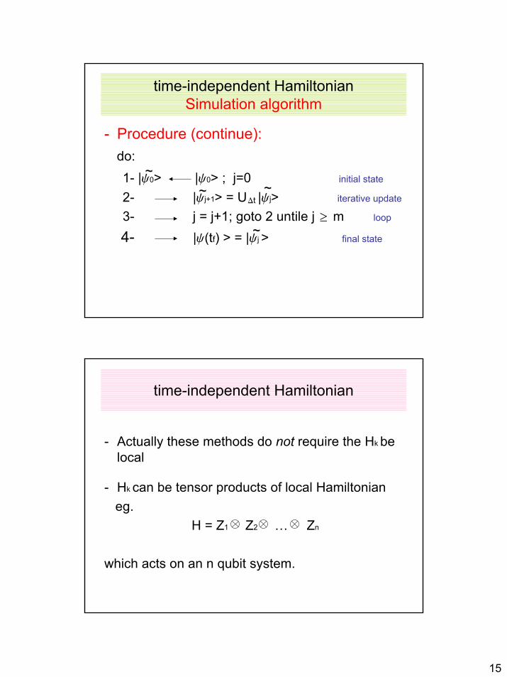
15
time-independent HamiltonianSimulation algorithm
- Procedure (continue): do: 1- |y0> |y0> ; j=0 initial state
2- |yj+1> = U |yj> iterative update
3- j = j+1; goto 2 untile j m loop
4- |y(tf) > = |yj > final state
~~ ~
≥~
Dt
time-independent Hamiltonian
- Actually these methods do not require the Hk be local
- Hk can be tensor products of local Hamiltonian eg.
H = Z1 Z2 … Zn
which acts on an n qubit system.
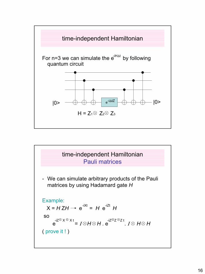
16
time-independent Hamiltonian
For n=3 we can simulate the e by following quantum circuit
H = Z1 Z2 Z3
-iHDt
e -iDtZ|0> |0>
time-independent HamiltonianPauli matrices
- We can simulate arbitrary products of the Paulimatrices by using Hadamard gate H
Example:X = H ZH e = H e H
so e = I H H . e . I H H
( prove it ! )
-iXt -iZt
-iZ X X t -iZ Z Z t
17
Exercise
Ex. 4.46; 4.47; 4.49; 4.50; 4.51
1
The quantum Fourier transform and its application
(Chapter 5)5.1 The quantum Fourier transform5.2 Phase estimation
5.2.1 Performance and requirements5.3 Applications: order-finding and factoring
5.3.1 Application: order-finding5.3.2. Application: factoring
Natural Fourier Transformer
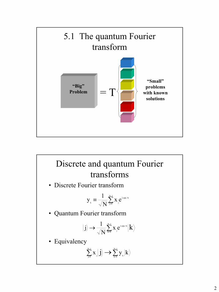
2
5.1 The quantum Fourier transform
= T“Big”
Problem
“Small” problems
with known solutions
Discrete and quantum Fourier transforms
• Discrete Fourier transform
• Quantum Fourier transform
• Equivalency
∑−
=≡
1N
0j
N/ijk2
jkex
N1y π
k1N
0k
N/ijk2
jex
N1j ∑
−
=→ π
kyx1N
0k k
1N
0j jj ∑→∑
−
=
−
=
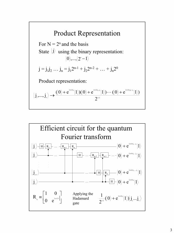
3
Product RepresentationFor N = 2n and the basisState using the binary representation:
j = j1j2 … jn = j12n-1 + j22n-2 + … + jn20
Product representation:
12,...,0 n −
j
2/n
jjj0i2jj0i2j0i2
n1 2)1e0()1e0)(1e0(j,...,j
n21n1nn ⋅⋅⋅⋅⋅⋅
+⋅⋅⋅++→
− πππ
Efficient circuit for the quantum Fourier transform
H R2 … Rn-1 Rn
H… Rn-2… Rn-1
H R2…
H
.
.
.
.
.
.
…
1j
2j
1nj
−
nj
1e0 n1 j...j0i2 ⋅
+π
1e0 n2 j...j0i2 ⋅
+π
…
1e0 n1n j...j0i2 −⋅
+π
1e0 nj0i2 ⋅
+π
≡ k2/i2k e001
R πn2
j0i2
2/1j...j)1e0(
21 1⋅+
πApplying the Hadamard gate
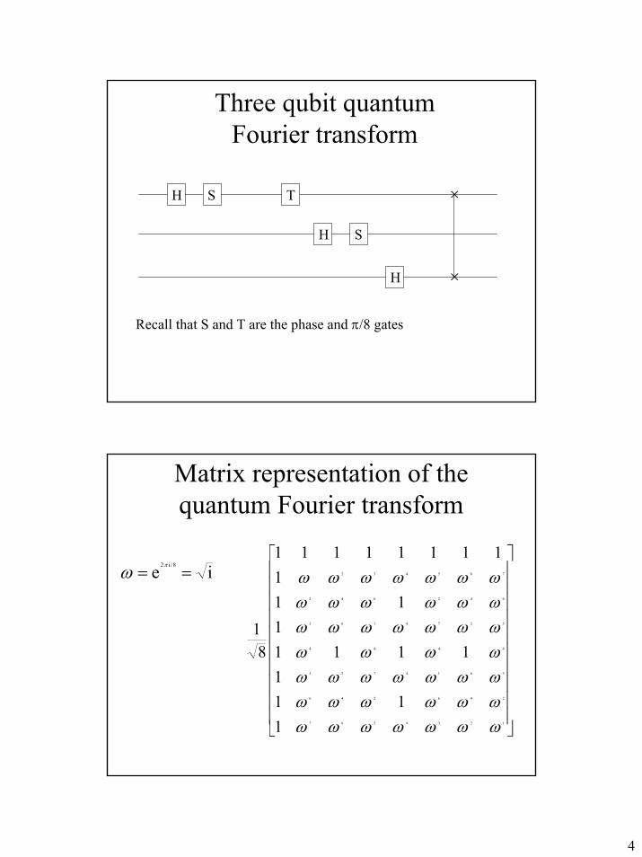
4
Three qubit quantum Fourier transform
H S T
H S
H
×
×
Recall that S and T are the phase and π/8 gates
Matrix representation of the quantum Fourier transform
1234567
246246
3614725
4444
5274163
642642
765432
111
11111
111
111111111
81
ωωωωωωωωωωωωωωωωωωωωωωωωωωωωωωωωωωωωωωωωωωωωie 8/i2
==πω
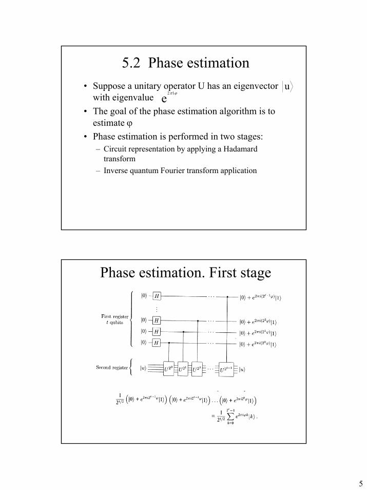
5
5.2 Phase estimation• Suppose a unitary operator U has an eigenvector
with eigenvalue • The goal of the phase estimation algorithm is to
estimate ϕ• Phase estimation is performed in two stages:
– Circuit representation by applying a Hadamard transform
– Inverse quantum Fourier transform application
uϕπ12e
Phase estimation. First stage
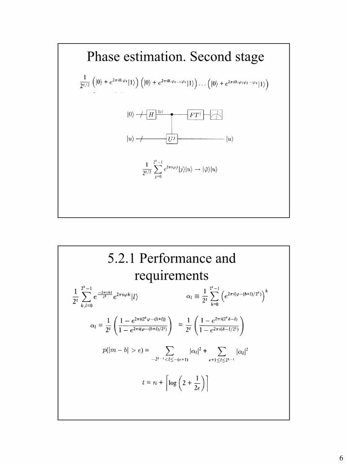
6
Phase estimation. Second stage
5.2.1 Performance and requirements
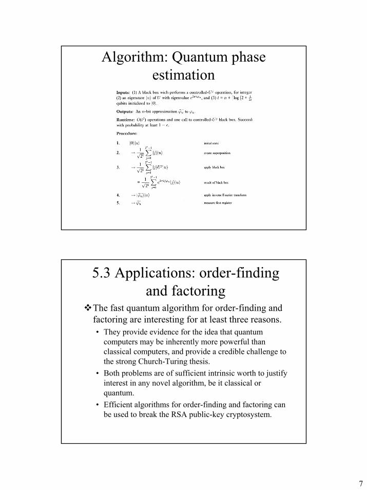
7
Algorithm: Quantum phase estimation
5.3 Applications: order-finding and factoring
The fast quantum algorithm for order-finding and factoring are interesting for at least three reasons.• They provide evidence for the idea that quantum
computers may be inherently more powerful than classical computers, and provide a credible challenge to the strong Church-Turing thesis.
• Both problems are of sufficient intrinsic worth to justify interest in any novel algorithm, be it classical or quantum.
• Efficient algorithms for order-finding and factoring can be used to break the RSA public-key cryptosystem.
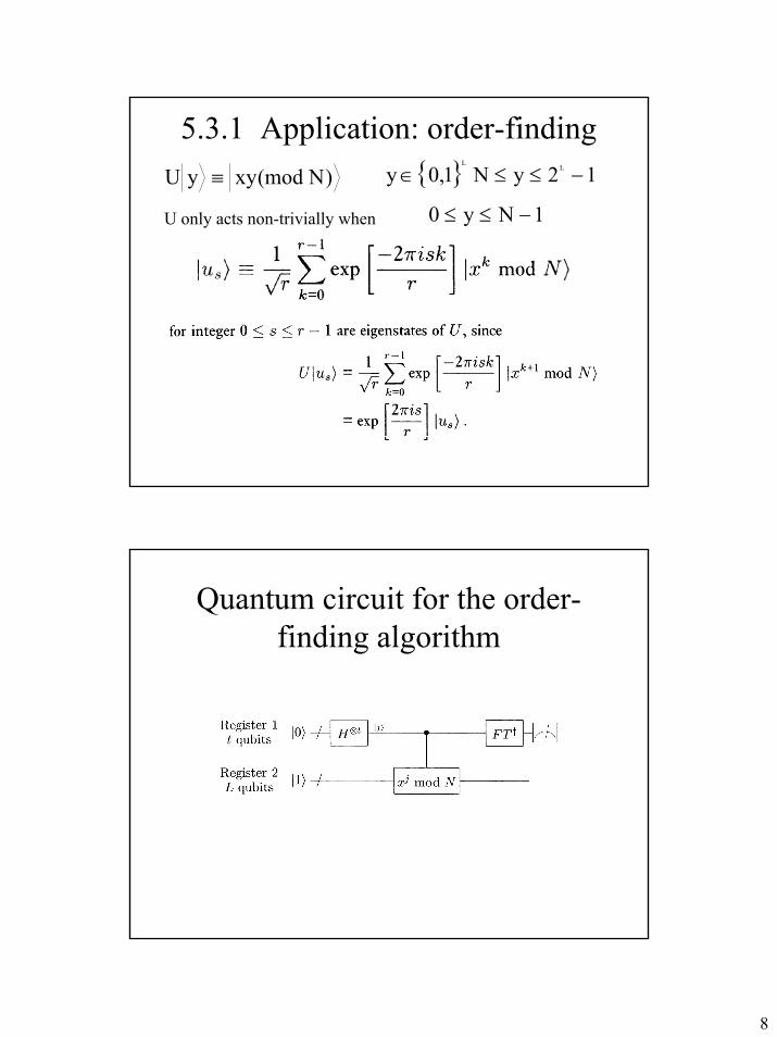
8
5.3.1 Application: order-finding
U only acts non-trivially when 1Ny0 −≤≤
)N(modxyyU ≡ 12yN1,0y LL
−≤≤∈
Quantum circuit for the order-finding algorithm
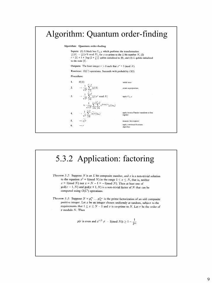
9
Algorithm: Quantum order-finding
5.3.2 Application: factoring
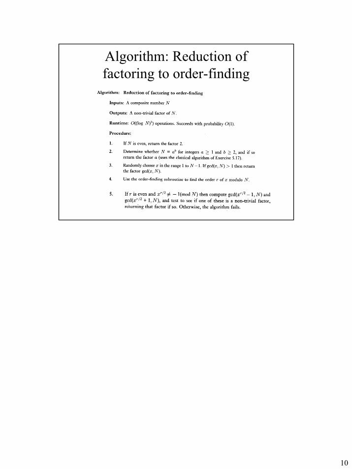
10
Algorithm: Reduction of factoring to order-finding
1
June 6, 2002 University of Alberta * QCSS * Summer 2002 * © Vadim Bulitko 1
QCSS
“Quantum Computing Summer School”
QCSSQCSS
“Quantum Computing “Quantum Computing Summer School”Summer School”
Prof. Vadim BulitkoUniversity of AlbertaProf. Vadim BulitkoProf. Vadim BulitkoUniversity of AlbertaUniversity of Alberta
June 6, 2002 University of Alberta * QCSS * Summer 2002 * © Vadim Bulitko 2
TodayTodayToday
• Summary of Chapter 4
• CS questions on QC
• Fourier transform re-cap
• Fourier transform applications– Period-finding
– Discrete logarithms
– The hidden subgroup problem
• Discussion
Jean Baptiste Joseph Fourier
Peter Shor
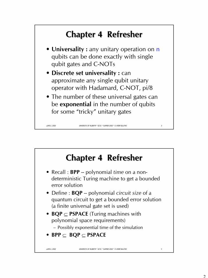
2
June 6, 2002 University of Alberta * QCSS * Summer 2002 * © Vadim Bulitko 3
Chapter 4 RefresherChapter 4 RefresherChapter 4 Refresher
• Universality : any unitary operation on n qubits can be done exactly with single qubit gates and C-NOTs
• Discrete set universality : can approximate any single qubit unitary operator with Hadamard, C-NOT, pi/8
• The number of these universal gates can be exponential in the number of qubits for some “tricky” unitary gates
June 6, 2002 University of Alberta * QCSS * Summer 2002 * © Vadim Bulitko 4
Chapter 4 RefresherChapter 4 RefresherChapter 4 Refresher• Recall : BPP -- polynomial time on a non-
deterministic Turing machine to get a bounded error solution
• Define : BQP -- polynomial circuit size of a quantum circuit to get a bounded error solution (a finite universal gate set is used)
• BQP ⊆ PSPACE (Turing machines with polynomial space requirements)– Possibly exponential time of the simulation
• BPP ⊆ BQP ⊆ PSPACE
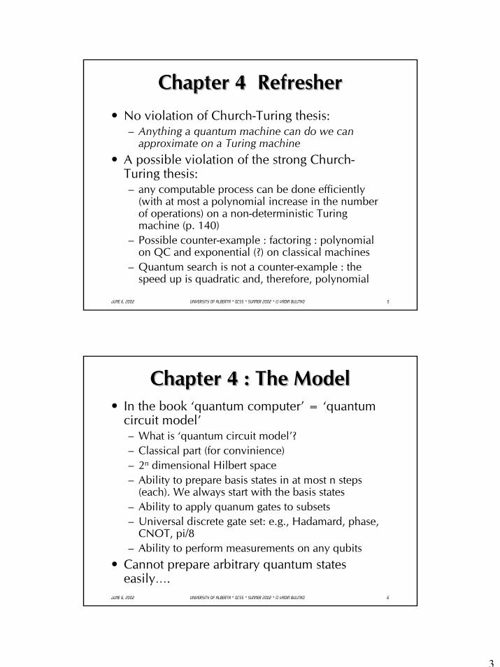
3
June 6, 2002 University of Alberta * QCSS * Summer 2002 * © Vadim Bulitko 5
Chapter 4 RefresherChapter 4 RefresherChapter 4 Refresher• No violation of Church-Turing thesis:
– Anything a quantum machine can do we can approximate on a Turing machine
• A possible violation of the strong Church-Turing thesis:– any computable process can be done efficiently
(with at most a polynomial increase in the number of operations) on a non-deterministic Turing machine (p. 140)
– Possible counter-example : factoring : polynomial on QC and exponential (?) on classical machines
– Quantum search is not a counter-example : the speed up is quadratic and, therefore, polynomial
June 6, 2002 University of Alberta * QCSS * Summer 2002 * © Vadim Bulitko 6
Chapter 4 : The ModelChapter 4 : The ModelChapter 4 : The Model• In the book ‘quantum computer’ = ‘quantum
circuit model’– What is ‘quantum circuit model’?– Classical part (for convinience)– 2n dimensional Hilbert space– Ability to prepare basis states in at most n steps
(each). We always start with the basis states– Ability to apply quanum gates to subsets– Universal discrete gate set: e.g., Hadamard, phase,
CNOT, pi/8– Ability to perform measurements on any qubits
• Cannot prepare arbitrary quantum states easily….
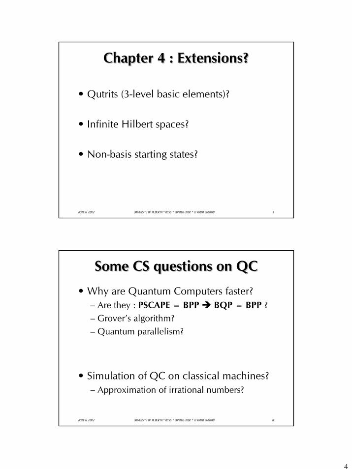
4
June 6, 2002 University of Alberta * QCSS * Summer 2002 * © Vadim Bulitko 7
Chapter 4 : Extensions?Chapter 4 : Extensions?Chapter 4 : Extensions?
• Qutrits (3-level basic elements)?
• Infinite Hilbert spaces?
• Non-basis starting states?
June 6, 2002 University of Alberta * QCSS * Summer 2002 * © Vadim Bulitko 8
Some CS questions on QCSome CS questions on QCSome CS questions on QC
• Why are Quantum Computers faster?– Are they : PSCAPE = BPP BQP = BPP ?– Grover’s algorithm?– Quantum parallelism?
• Simulation of QC on classical machines?– Approximation of irrational numbers?
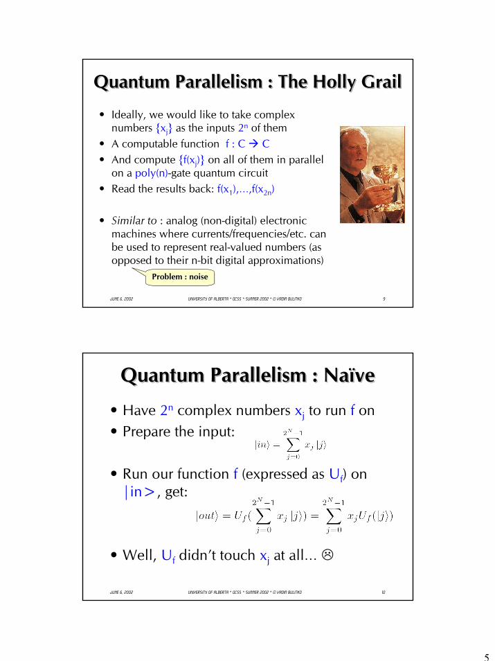
5
June 6, 2002 University of Alberta * QCSS * Summer 2002 * © Vadim Bulitko 9
Quantum Parallelism : The Holly GrailQuantum Parallelism : The Holly GrailQuantum Parallelism : The Holly Grail
• Ideally, we would like to take complex numbers xj as the inputs 2n of them
• A computable function f : C C• And compute f(xj) on all of them in parallel
on a poly(n)-gate quantum circuit• Read the results back: f(x1),…,f(x2n)
• Similar to : analog (non-digital) electronic machines where currents/frequencies/etc. can be used to represent real-valued numbers (as opposed to their n-bit digital approximations)
Problem : noiseProblem : noiseProblem : noise
June 6, 2002 University of Alberta * QCSS * Summer 2002 * © Vadim Bulitko 10
Quantum Parallelism : Naïve Quantum Parallelism : Naïve Quantum Parallelism : Naïve
• Have 2n complex numbers xj to run f on • Prepare the input:
• Run our function f (expressed as Uf) on |in>, get:
• Well, Uf didn’t touch xj at all…
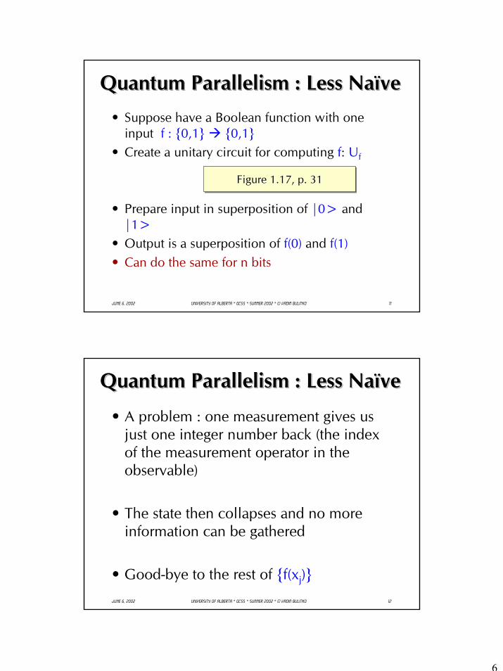
6
June 6, 2002 University of Alberta * QCSS * Summer 2002 * © Vadim Bulitko 11
Quantum Parallelism : Less Naïve Quantum Parallelism : Less Naïve Quantum Parallelism : Less Naïve • Suppose have a Boolean function with one
input f : 0,1 0,1• Create a unitary circuit for computing f: Uf
• Prepare input in superposition of |0> and |1>
• Output is a superposition of f(0) and f(1)• Can do the same for n bits
Figure 1.17, p. 31Figure 1.17, p. 31Figure 1.17, p. 31
June 6, 2002 University of Alberta * QCSS * Summer 2002 * © Vadim Bulitko 12
Quantum Parallelism : Less Naïve Quantum Parallelism : Less Naïve Quantum Parallelism : Less Naïve
• A problem : one measurement gives us just one integer number back (the index of the measurement operator in the observable)
• The state then collapses and no more information can be gathered
• Good-bye to the rest of f(xj)
7
June 6, 2002 University of Alberta * QCSS * Summer 2002 * © Vadim Bulitko 13
What can we do?What What cancan we do?we do?• Well, we can measure some global properties
of f fast…• Example #1 : Deutsch’s algorithm (p. 33): can
measure f(0) XOR f(1) with a single Uf circuit run.
• Example #2 : Deutsch-Jozsa’s algorithm : can determine if f is balanced/constant in poly(n)steps where as need O(exp(n)) evaluations of fin the classical case (p. 34)
• Problems --- Eric?
June 6, 2002 University of Alberta * QCSS * Summer 2002 * © Vadim Bulitko 14
Quantum Parallelism : Question Quantum Parallelism : Question Quantum Parallelism : Question • We seem unable to use amplitudes of the basis
vectors (even normalized) to encode inputs xj• …because any quantum gate is linear and will
simply pass them through• The solution suggested was to encode xj in
binary (n bits) and use basis vectors (for nqubits) to represent all of them.
• Here is a question : Can we use phases of vectors to encode xj ?
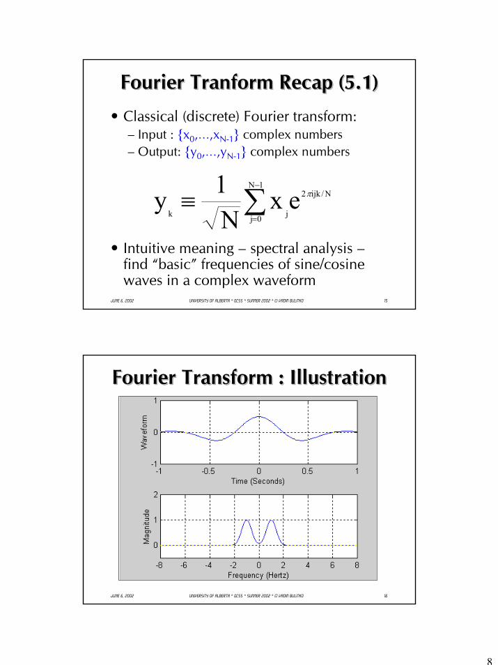
8
June 6, 2002 University of Alberta * QCSS * Summer 2002 * © Vadim Bulitko 15
Fourier Tranform Recap (5.1)Fourier Tranform Recap (5.1)Fourier Tranform Recap (5.1)
• Classical (discrete) Fourier transform:– Input : x0,…,xN-1 complex numbers– Output: y0,…,yN-1 complex numbers
• Intuitive meaning – spectral analysis –find “basic” frequencies of sine/cosine waves in a complex waveform
∑−
=≡
1N
0j
N/ijk2
jkex
N1y π
June 6, 2002 University of Alberta * QCSS * Summer 2002 * © Vadim Bulitko 16
Fourier Transform : IllustrationFourier Transform : IllustrationFourier Transform : Illustration
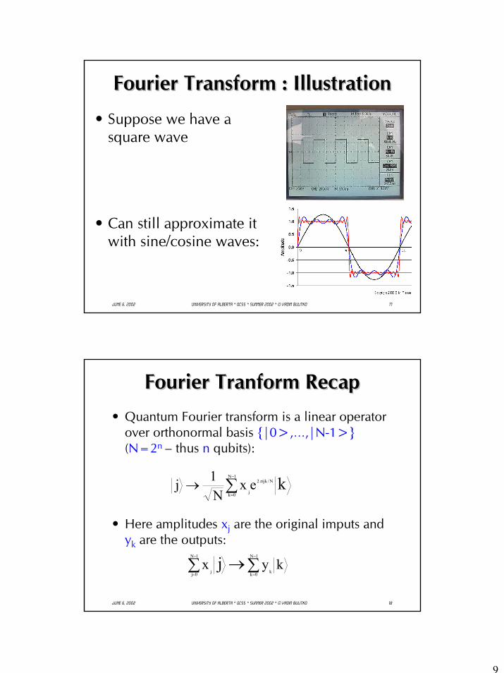
9
June 6, 2002 University of Alberta * QCSS * Summer 2002 * © Vadim Bulitko 17
Fourier Transform : IllustrationFourier Transform : IllustrationFourier Transform : Illustration
• Suppose we have a square wave
• Can still approximate it with sine/cosine waves:
June 6, 2002 University of Alberta * QCSS * Summer 2002 * © Vadim Bulitko 18
Fourier Tranform RecapFourier Tranform RecapFourier Tranform Recap• Quantum Fourier transform is a linear operator
over orthonormal basis |0>,…,|N-1>(N=2n – thus n qubits):
• Here amplitudes xj are the original imputs and yk are the outputs:
k1N
0k
N/ijk2
jex
N1j ∑
−
=→ π
kyx1N
0k k
1N
0j jj ∑→∑
−
=
−
=
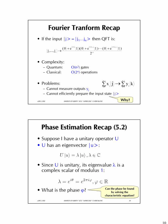
10
June 6, 2002 University of Alberta * QCSS * Summer 2002 * © Vadim Bulitko 19
Fourier Tranform RecapFourier Tranform RecapFourier Tranform Recap• If the input |j>=|j1…jn> then QFT is:
• Complexity:– Quantum: O(n2) gates– Classical: O(2n) operations
• Problems:– Cannot measure outputs yj
– Cannot efficiently prepare the input state |j>
2/n
jjj0i2jj0i2j0i2
n1 2)1e0()1e0)(1e0(j,...,j
n21n1nn ⋅⋅⋅⋅⋅⋅
+⋅⋅⋅++→
− πππ
kyx1N
0k k
1N
0j jj ∑→∑
−
=
−
=
Why?Why?Why?
June 6, 2002 University of Alberta * QCSS * Summer 2002 * © Vadim Bulitko 20
Phase Estimation Recap (5.2)Phase Estimation Recap (5.2)Phase Estimation Recap (5.2)
• Suppose I have a unitary operator U• U has an eigenvector |u>:
• Since U is unitary, its eigenvalue λ is a complex scalar of modulus 1:
• What is the phase ϕ? Can the phase be found by solving the
characteristic equation?
Can the phase be found Can the phase be found by solving the by solving the
characteristic equation?characteristic equation?
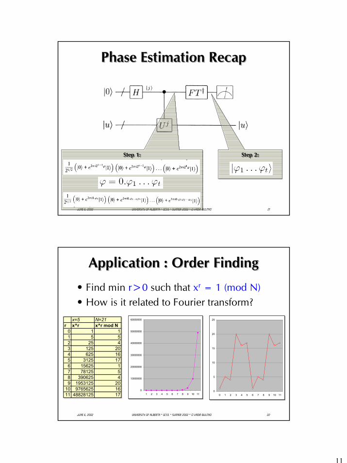
11
June 6, 2002 University of Alberta * QCSS * Summer 2002 * © Vadim Bulitko 21
Phase Estimation RecapPhase Estimation RecapPhase Estimation Recap
Step 1: Step 1: Step 1: Step 2: Step 2: Step 2:
June 6, 2002 University of Alberta * QCSS * Summer 2002 * © Vadim Bulitko 22
Application : Order FindingApplication : Order FindingApplication : Order Finding
• Find min r>0 such that xr = 1 (mod N)• How is it related to Fourier transform?
0
10000000
20000000
30000000
40000000
50000000
60000000
1 2 3 4 5 6 7 8 9 10 11
0
10000000
20000000
30000000
40000000
50000000
60000000
1 2 3 4 5 6 7 8 9 10 110
5
10
15
20
25
0 1 2 3 4 5 6 7 8 9 10 110
5
10
15
20
25
0 1 2 3 4 5 6 7 8 9 10 11
x=5 N=21r x^r x^r mod N0 1 11 5 52 25 43 125 204 625 165 3125 176 15625 17 78125 58 390625 49 1953125 2010 9765625 1611 48828125 17
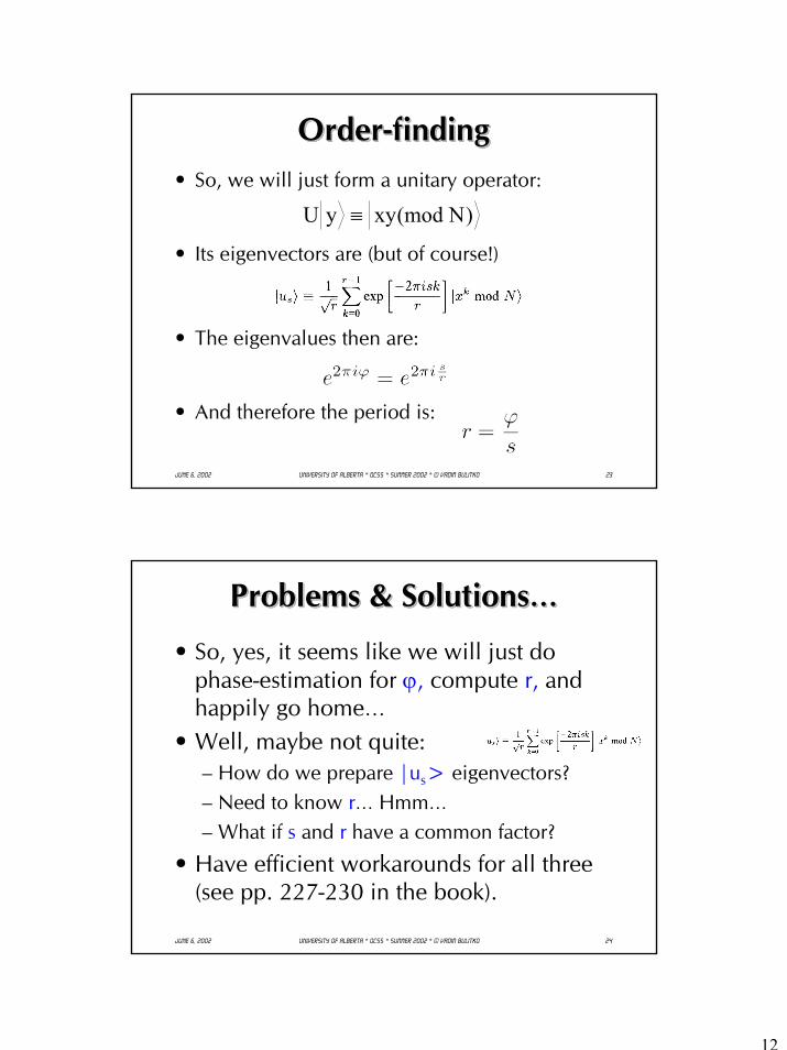
12
June 6, 2002 University of Alberta * QCSS * Summer 2002 * © Vadim Bulitko 23
Order-findingOrderOrder--findingfinding• So, we will just form a unitary operator:
• Its eigenvectors are (but of course!)
• The eigenvalues then are:
• And therefore the period is:
)N(modxyyU ≡
June 6, 2002 University of Alberta * QCSS * Summer 2002 * © Vadim Bulitko 24
Problems & Solutions… Problems & Solutions… Problems & Solutions…
• So, yes, it seems like we will just do phase-estimation for ϕ, compute r, and happily go home…
• Well, maybe not quite:– How do we prepare |us> eigenvectors?– Need to know r… Hmm… – What if s and r have a common factor?
• Have efficient workarounds for all three (see pp. 227-230 in the book).
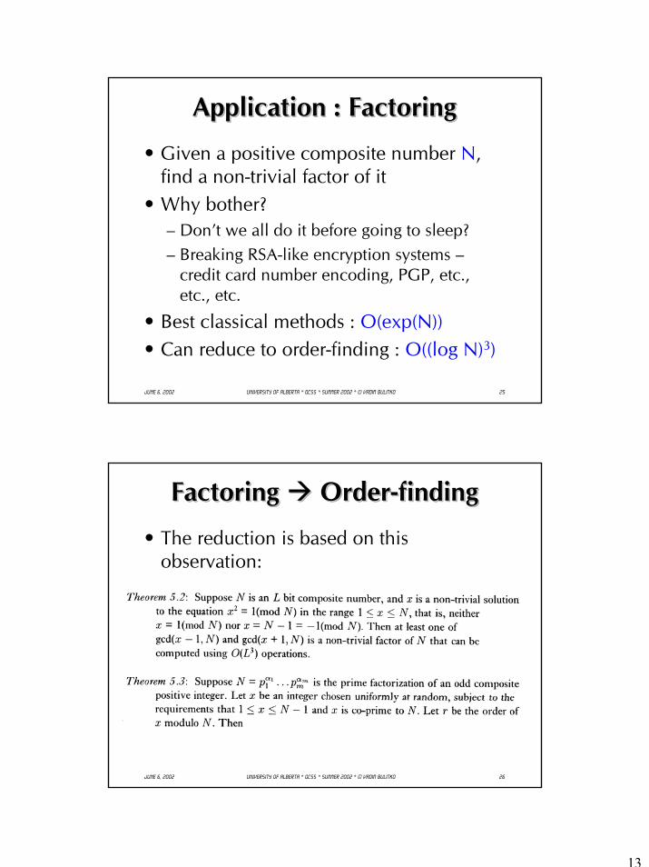
13
June 6, 2002 University of Alberta * QCSS * Summer 2002 * © Vadim Bulitko 25
Application : FactoringApplication : FactoringApplication : Factoring
• Given a positive composite number N, find a non-trivial factor of it
• Why bother?– Don’t we all do it before going to sleep?– Breaking RSA-like encryption systems –
credit card number encoding, PGP, etc., etc., etc.
• Best classical methods : O(exp(N))• Can reduce to order-finding : O((log N)3)
June 6, 2002 University of Alberta * QCSS * Summer 2002 * © Vadim Bulitko 26
Factoring Order-findingFactoring Factoring OrderOrder--findingfinding
• The reduction is based on this observation:
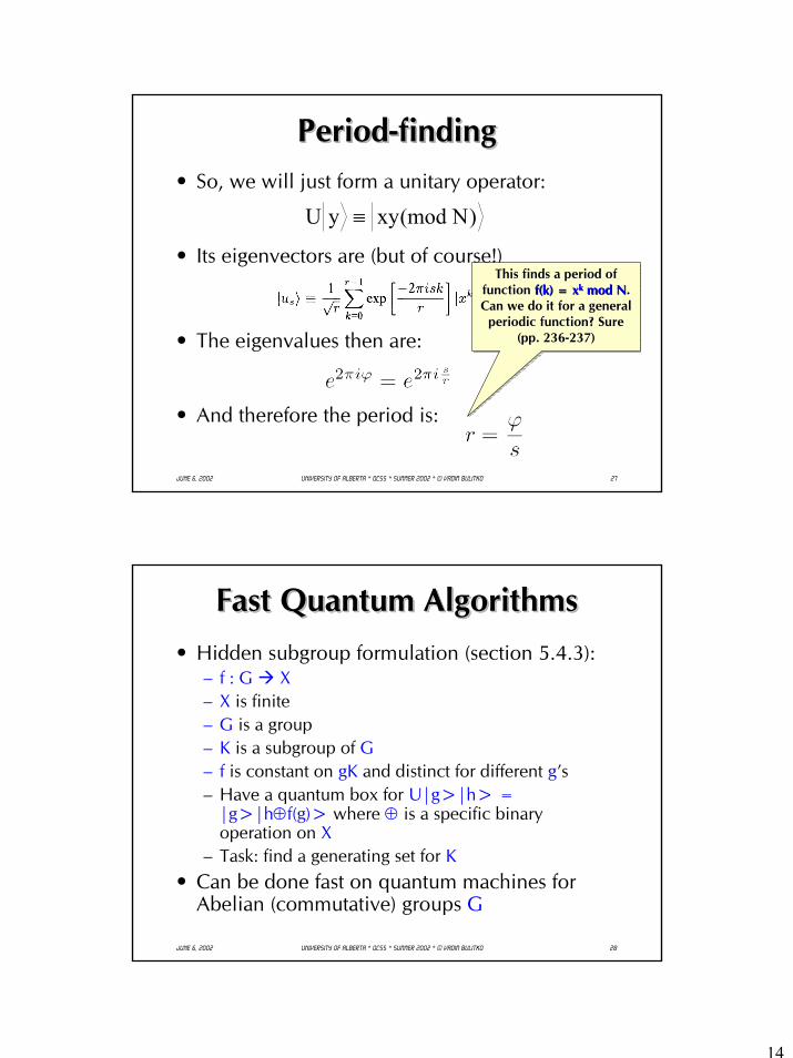
14
June 6, 2002 University of Alberta * QCSS * Summer 2002 * © Vadim Bulitko 27
Period-findingPeriodPeriod--findingfinding• So, we will just form a unitary operator:
• Its eigenvectors are (but of course!)
• The eigenvalues then are:
• And therefore the period is:
)N(modxyyU ≡
This finds a period of function f(k) = xk mod N. Can we do it for a general
periodic function? Sure (pp. 236-237)
This finds a period of This finds a period of function function f(k) = xf(k) = xkk mod Nmod N. . Can we do it for a general Can we do it for a general
periodic function? Sure periodic function? Sure (pp. 236(pp. 236--237) 237)
June 6, 2002 University of Alberta * QCSS * Summer 2002 * © Vadim Bulitko 28
Fast Quantum AlgorithmsFast Quantum AlgorithmsFast Quantum Algorithms• Hidden subgroup formulation (section 5.4.3):
– f : G X– X is finite– G is a group– K is a subgroup of G– f is constant on gK and distinct for different g’s– Have a quantum box for U|g>|h> =
|g>|h⊕f(g)> where ⊕ is a specific binary operation on X
– Task: find a generating set for K• Can be done fast on quantum machines for
Abelian (commutative) groups G
15
June 6, 2002 University of Alberta * QCSS * Summer 2002 * © Vadim Bulitko 29
The Power of QCThe Power of QCThe Power of QC
• Again : What makes QC appear faster than classical machines?
– Parallelism?
– Promise (e.g., existence of generating subset for K)
• Question: why do we need a promise?
June 6, 2002 University of Alberta * QCSS * Summer 2002 * © Vadim Bulitko 30
Check - pointCheck Check -- pointpoint
• Done with these : – Chapter 1 : Intro– Chapter 2 : Linear Algebra + postulates– Chapter 3 : Computer Science– Chapter 4 : Quantum Circuits– Chapter 5 : Quantum Fourier Transform
• Now on to:– Chapter 6 : Quantum Search– Chapter 7 : Physical Realization of QMs
Why are Q
C faster?
How
can youapply Q
C in your area?
Why are Q
C faster?
Why are Q
C faster?
How
can H
ow can you
youapply Q
C in your area?
apply QC
in your area?
1
Chapter 6
QUANTUM SEARCH ALGORITHM
Lecture 12
Vahid RezaniaMay-June 2002
Overview
• The algorithm
• Quantum counting
• Search as quantum simulation
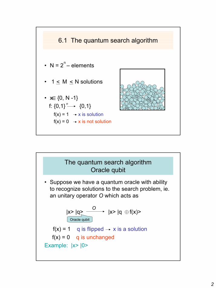
2
6.1 The quantum search algorithm
• N = 2 – elements
• 1 M N solutions
• x 0, N -1f: 0,1 0,1
f(x) = 1 x is solutionf(x) = 0 x is not solution
02
1
463
5510
3
n
__ < __ <
∈n
The quantum search algorithmOracle qubit
• Suppose we have a quantum oracle with ability to recognize solutions to the search problem, ie. an unitary operator O which acts as
|x> |q> |x> |q f(x)>
f(x) = 1 q is flipped x is a solutionf(x) = 0 q is unchanged
Example: |x> |0>
O
Oracle qubit
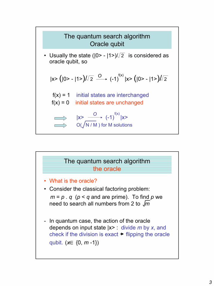
3
The quantum search algorithmOracle qubit
• Usually the state (|0> - |1>)/ 2 is considered as oracle qubit, so
|x> (|0> - |1>)/ 2 (-1) |x> (|0> - |1>)/ 2
f(x) = 1 initial states are interchangedf(x) = 0 initial states are unchanged
|x> (-1) |x>O( N / M ) for M solutions
O f(x)
O f(x)
The quantum search algorithmthe oracle
• What is the oracle?• Consider the classical factoring problem:
m = p . q (p < q and are prime). To find p we need to search all numbers from 2 to m
- In quantum case, the action of the oracle depends on input state |x> : divide m by x, and check if the division is exact flipping the oracle qubit. (x 0, m -1)∈
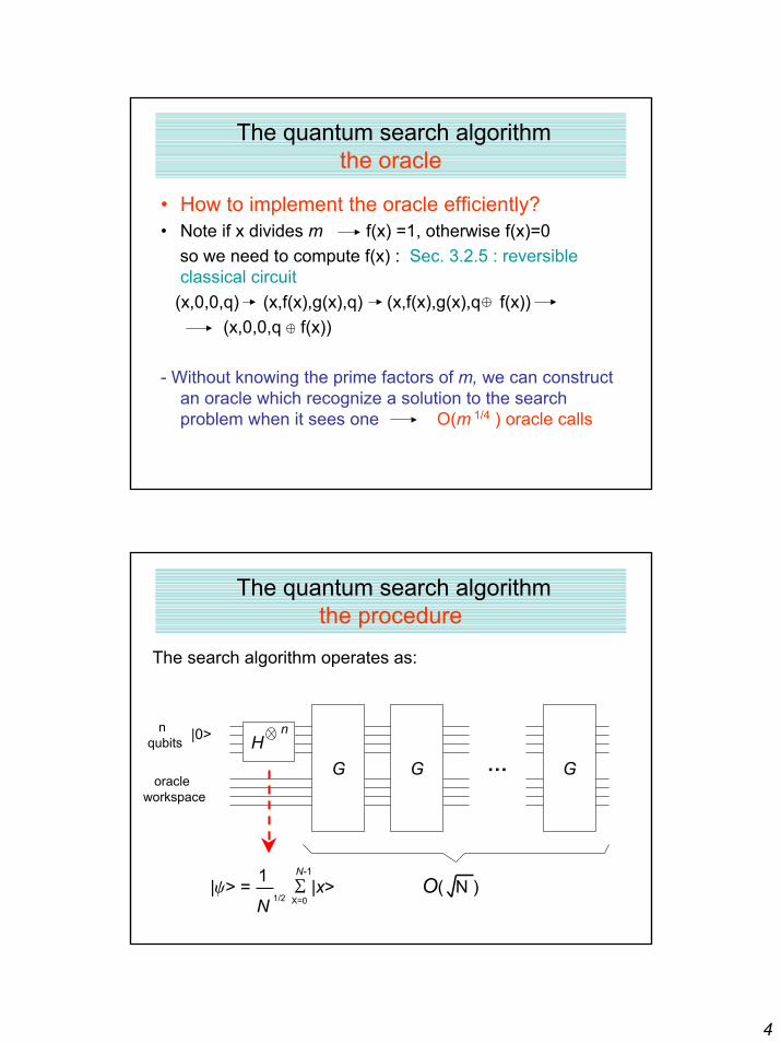
4
The quantum search algorithmthe oracle
• How to implement the oracle efficiently? • Note if x divides m f(x) =1, otherwise f(x)=0
so we need to compute f(x) : Sec. 3.2.5 : reversible classical circuit
(x,0,0,q) (x,f(x),g(x),q) (x,f(x),g(x),q f(x)) (x,0,0,q f(x))
- Without knowing the prime factors of m, we can construct an oracle which recognize a solution to the search problem when it sees one O(m ) oracle calls1/4
The quantum search algorithmthe procedure
The search algorithm operates as:
|y> = S |x> O( N )
|0> H n
G G G…
nqubits
oracleworkspace
1
N 1/2 X=0
N-1
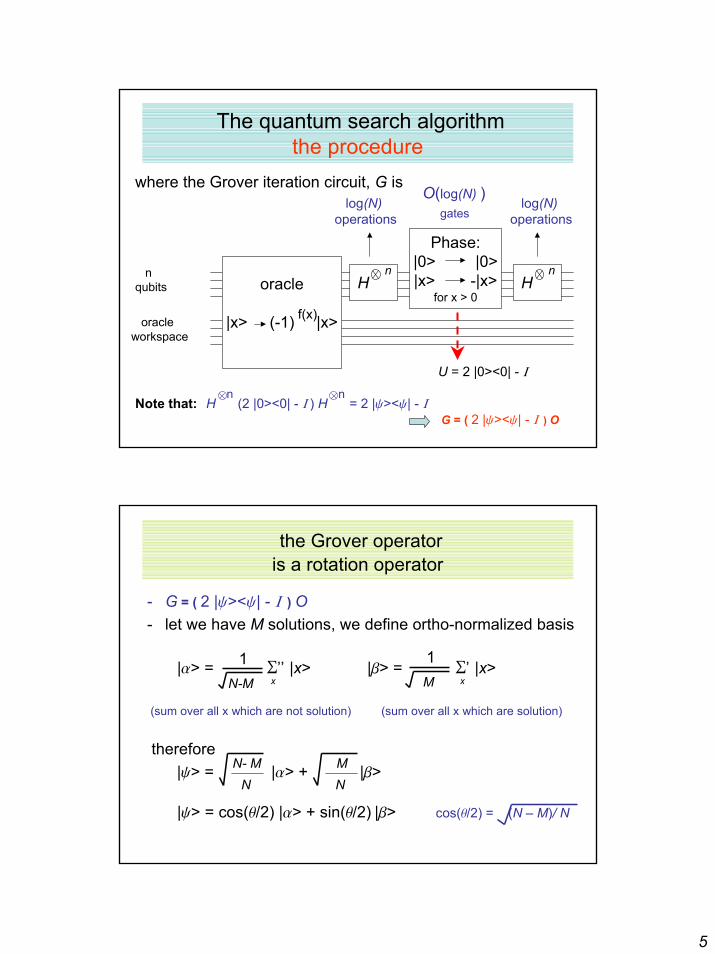
5
The quantum search algorithmthe procedure
where the Grover iteration circuit, G is
U = 2 |0><0| - I
Note that: H (2 |0><0| - I ) H = 2 |y><y| - IG = ( 2 |y><y| - I ) O
log(N) operations
oracleworkspace
H n
oracle
|x> (-1) |x>
nqubits
f(x)
H n
Phase:|0> |0>|x> -|x>
for x > 0
log(N)operations
O(log(N) ) gates
n n
the Grover operatoris a rotation operator
- G = ( 2 |y><y| - I ) O- let we have M solutions, we define ortho-normalized basis
|a> = S’’ |x> |b> = S’ |x>
(sum over all x which are not solution) (sum over all x which are solution)
therefore|y> = |a> + |b>
|y> = cos(q/2) |a> + sin(q/2) |b> cos(q/2) = (N – M)/ N
1N-M x
1M x
N- MN
MN
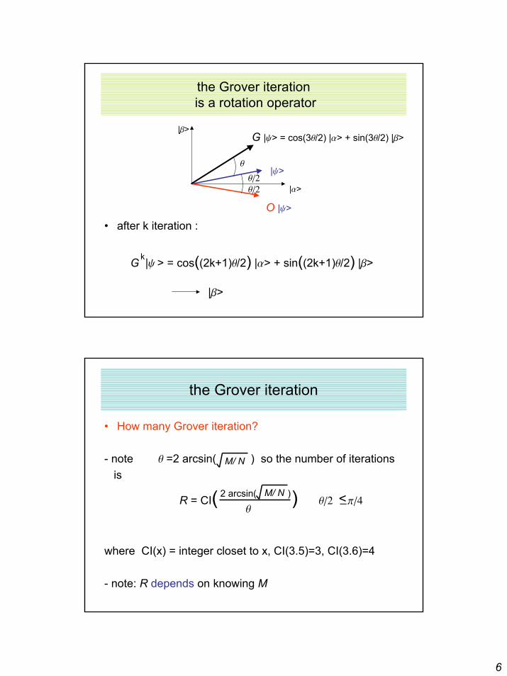
6
the Grover iterationis a rotation operator
• after k iteration :
G |y > = cos((2k+1)q/2) |a> + sin((2k+1)q/2) |b>
|b>
|b>
|a>
G |y> = cos(3q/2) |a> + sin(3q/2) |b>
|y>
O |y>
q
q/2q/2
k
the Grover iteration
• How many Grover iteration?
- note q =2 arcsin( ) so the number of iterations is
R = CI( ) q/2 p/4
where CI(x) = integer closet to x, CI(3.5)=3, CI(3.6)=4
- note: R depends on knowing M
M/ N
2 arcsin( )M/ N
q<_
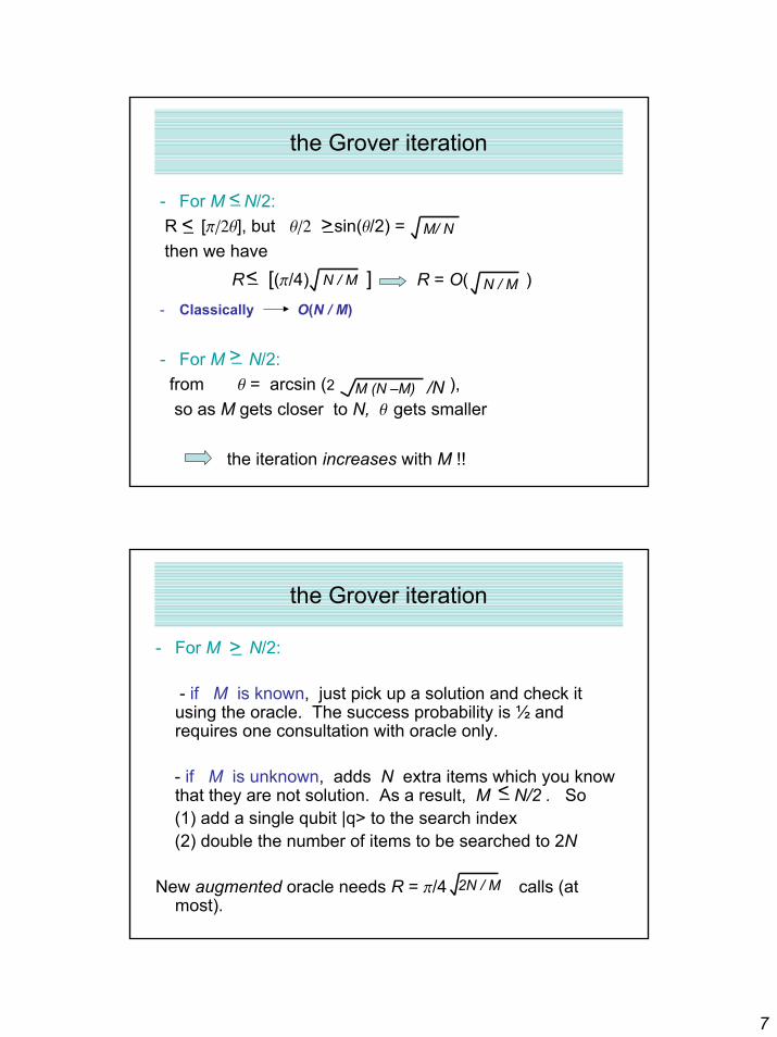
7
the Grover iteration
- For M N/2:R [p/2q], but q/2 sin(q/2) = then we have
R [(p/4) ] R = O( )- Classically O(N / M)
- For M N/2:from q = arcsin (2 ), so as M gets closer to N, q gets smaller
the iteration increases with M !!
<_ >_ M/ N
<_ N / M N / M
<_
>_M (N –M) /N
the Grover iteration
- For M N/2:
- if M is known, just pick up a solution and check it using the oracle. The success probability is ½ and requires one consultation with oracle only.
- if M is unknown, adds N extra items which you know that they are not solution. As a result, M N/2 . So(1) add a single qubit |q> to the search index(2) double the number of items to be searched to 2N
New augmented oracle needs R = p/4 calls (at most).
>_
<_
2N / M
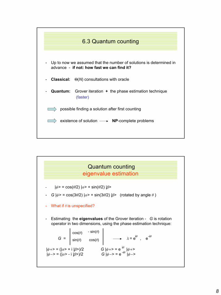
8
6.3 Quantum counting
- Up to now we assumed that the number of solutions is determined in advance - if not: how fast we can find it?
- Classical: Q(N) consultations with oracle
- Quantum: Grover iteration + the phase estimation technique (faster)
possible finding a solution after first counting
existence of solution NP-complete problems
Quantum countingeigenvalue estimation
- |y> = cos(q/2) |a> + sin(q/2) |b>
- G |y> = cos(3q/2) |a> + sin(3q/2) |b> (rotated by angle q )
- What if q is unspecified?
- Estimating the eigenvalues of the Grover iteration - G is rotationoperator in two dimensions, using the phase estimation technique:
G = l = e , e
|y+> = (|a> + i |b>)/2 G |y+> = e |y+> |y-> = (|a> - i |b>)/2 G |y-> = e |y->
cos(q)sin(q)
- sin(q)cos(q)iq -iq
iq-iq
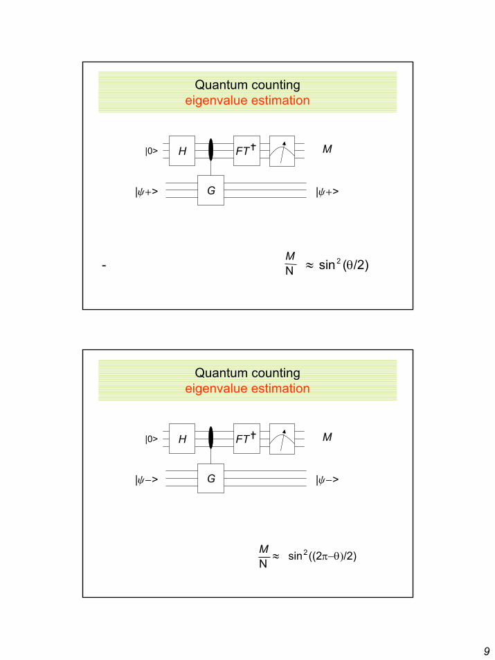
9
Quantum countingeigenvalue estimation
- ≈ sin (θ/2)
H FT
G
|0>
|y+>
M
|y+>
NM 2
Quantum countingeigenvalue estimation
≈ sin ((2π−θ)/2)
H FT
G
|0>
|y->
M
|y->
NM 2
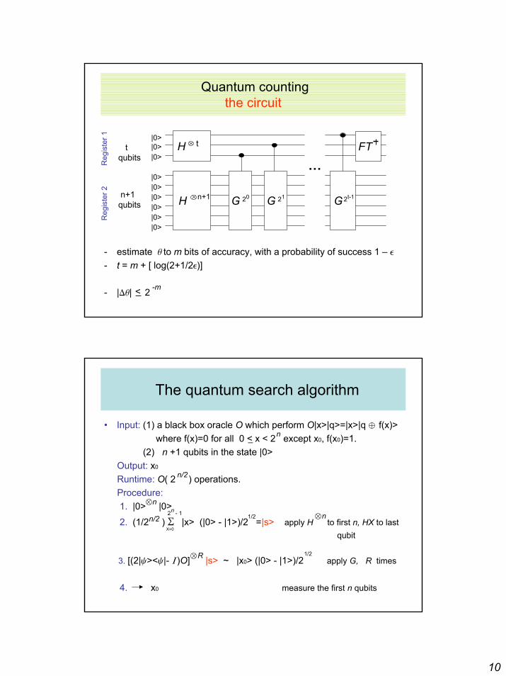
10
Quantum countingthe circuit
- estimate q to m bits of accuracy, with a probability of success 1 – e
- t = m + [ log(2+1/2e)]
- |Dq| 2
|0>H t
…t
qubits
n+1 qubits H G n+1 20 G 21 G 2t-1
FT |0>|0>
|0>|0>
|0>|0>
|0>|0>
Reg
iste
r 1R
egis
ter 2
<_ -m
The quantum search algorithm
• Input: (1) a black box oracle O which perform O|x>|q>=|x>|q f(x)> where f(x)=0 for all 0 < x < 2 except x0, f(x0)=1.
(2) n +1 qubits in the state |0>Output: x0
Runtime: O( 2 ) operations.Procedure: 1. |0> |0>2. (1/2 ) S |x> (|0> - |1>)/2 =|s> apply H to first n, HX to last
qubit
3. [(2|y><y|- I )O] |s> ~ |x0> (|0> - |1>)/2 apply G, R times
4. x0 measure the first n qubits
n_
n/2
n
n/2 1/2
X=0
2 - 1nn
R 1/2
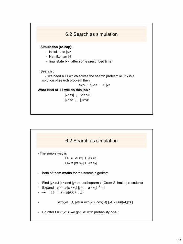
11
6.2 Search as simulation
Simulation (re-cap):- initial state |y>- Hamiltonian H- final state |x> after some prescribed time
Search :- we need a H which solves the search problem ie. if x is a
solution of search problem then exp(-iHt)|y> |x>
What kind of H will do this job?|x><x| , |y><y||x><y| , |y><x|
6.2 Search as simulation
- The simple way is H = |x><x| + |y><y|H = |x><y| + |y><x|
- both of them works for the search algorithm
- Find |y> s.t |x> and |y> are orthonormal (Gram-Schmidt procedure)- Expand |y> = a |x> + b |y> , a + b = 1- H = I + a(b X + a Z)
- exp(-iH t) |y> = exp(-it) [cos(at) |y> - i sin(at)|x>]
- So after t = p/(2a) we get |x> with probability one !
1
2
2 2
1
1
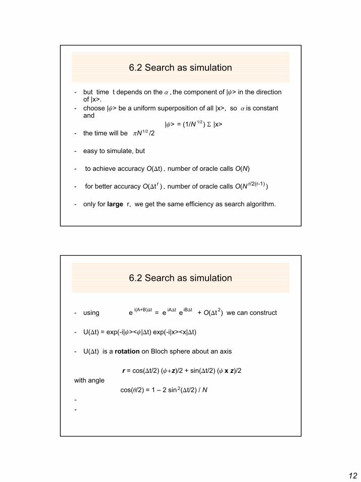
12
6.2 Search as simulation
- but time t depends on the a , the component of |y> in the direction of |x>.
- choose |y> be a uniform superposition of all |x>, so a is constant and
|y> = (1/N ) S |x>- the time will be pN /2
- easy to simulate, but
- to achieve accuracy O(Dt) , number of oracle calls O(N)
- for better accuracy O(Dt ) , number of oracle calls O(N )
- only for large r, we get the same efficiency as search algorithm.
1/2
1/2
r r/2(r-1)
6.2 Search as simulation
- using e = e e + O(Dt ) we can construct
- U(Dt) = exp(-i|y><y|Dt) exp(-i|x><x|Dt)
- U(Dt) is a rotation on Bloch sphere about an axis
r = cos(Dt/2) (y+z)/2 + sin(Dt/2) (y x z)/2 with angle
cos(q/2) = 1 – 2 sin (Dt/2) / N--
i(A+B)Dt iADt iBDt 2
2
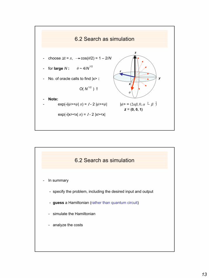
13
6.2 Search as simulation
- choose Dt = p, cos(q/2) = 1 – 2/N
- for large N : q ~ 4/N
- No. of oracle calls to find |x> :
O( N ) !
- Note: - exp(-i|y><y| p) = I - 2 |y><y| |y> = (2ab, 0, a - b )
z = (0, 0, 1)exp(-i|x><x| p) = I - 2 |x><x|
r
z
y
x
y
1/2
1/2
2 2
6.2 Search as simulation
- In summary
- specify the problem, including the desired input and output
- guess a Hamiltonian (rather than quantum circuit)
- simulate the Hamiltonian
- analyze the costs
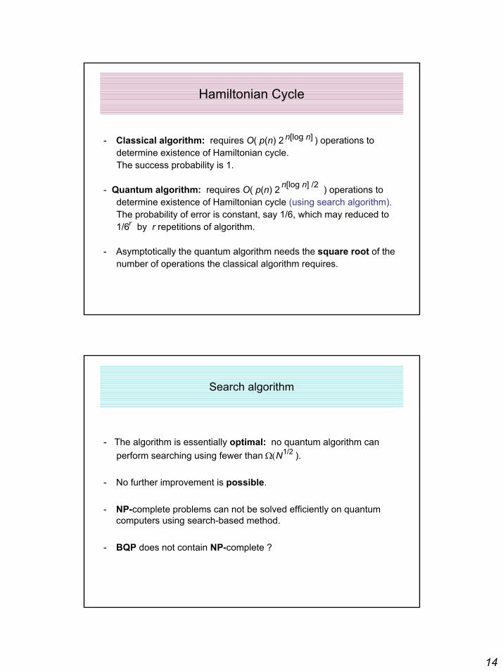
14
Hamiltonian Cycle
- Classical algorithm: requires O( p(n) 2 ) operations todetermine existence of Hamiltonian cycle. The success probability is 1.
- Quantum algorithm: requires O( p(n) 2 ) operations todetermine existence of Hamiltonian cycle (using search algorithm).The probability of error is constant, say 1/6, which may reduced to 1/6 by r repetitions of algorithm.
- Asymptotically the quantum algorithm needs the square root of the number of operations the classical algorithm requires.
n[log n]
n[log n] /2
r
Search algorithm
- The algorithm is essentially optimal: no quantum algorithm canperform searching using fewer than Ω(N ).
- No further improvement is possible.
- NP-complete problems can not be solved efficiently on quantum computers using search-based method.
- BQP does not contain NP-complete ?
1/2
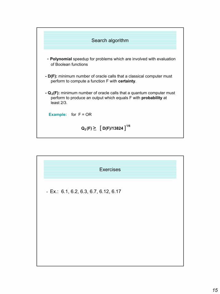
15
Search algorithm
- Polynomial speedup for problems which are involved with evaluation of Boolean functions
- D(F): minimum number of oracle calls that a classical computer must perform to compute a function F with certainty.
- Q (F): minimum number of oracle calls that a quantum computer must perform to produce an output which equals F with probability at least 2/3.
Example: for F = OR
Q (F) [ D(F)/13824 ]
2
21/6>_
Exercises
- Ex.: 6.1, 6.2, 6.3, 6.7, 6.12, 6.17
1
7. Quantum computers: physical realization
To be or not to be. That’s a question…William Shakespeare
The “classic” answers: “to be” or “not to be”The “quantum” answers:“to be”, “not to be” or a × (to be) + b × (not to be)
7. Quantum computers: physical realization(Outline)
• Section 7.1: An overview of the tradeoffs in selecting a physical realization of a quantum computer
• Section 7.2: Physical conditions for quantum computation • Section 7.3: Harmonic oscillator quantum computer• Section 7.4: Optical photon quantum computer• Section 7.5: Optical cavity quantum electrodynamics• Section 7.6: Ion traps• Section 7.7: Nuclear magnetic resonance (NMR)• Section 7.8: Other implementation schemes
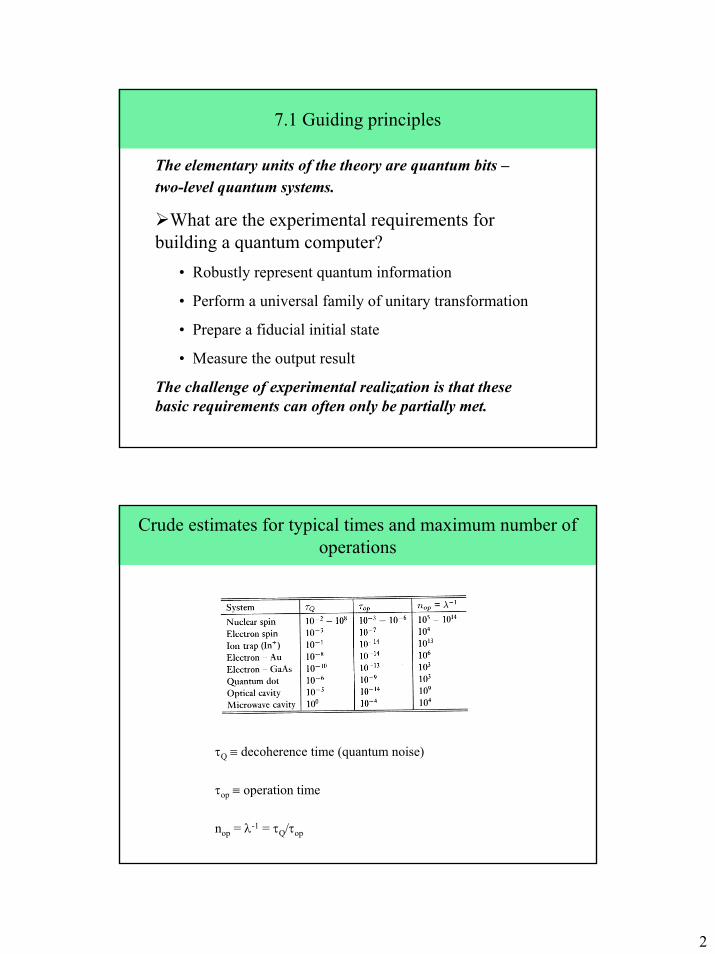
2
7.1 Guiding principles
The elementary units of the theory are quantum bits –two-level quantum systems.
What are the experimental requirements for building a quantum computer?
• Robustly represent quantum information
• Perform a universal family of unitary transformation
• Prepare a fiducial initial state
• Measure the output result
The challenge of experimental realization is that these basic requirements can often only be partially met.
Crude estimates for typical times and maximum number of operations
τQ ≡ decoherence time (quantum noise)
τop ≡ operation time
nop = λ-1 = τQ/τop
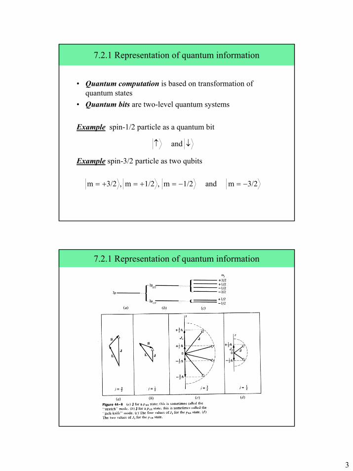
3
7.2.1 Representation of quantum information
• Quantum computation is based on transformation of quantum states
• Quantum bits are two-level quantum systems
Example spin-1/2 particle as a quantum bit
Example spin-3/2 particle as two qubits
↓↑ and
3/2mand1/2m,1/2m ,3/2m −=−=+=+=
7.2.1 Representation of quantum information
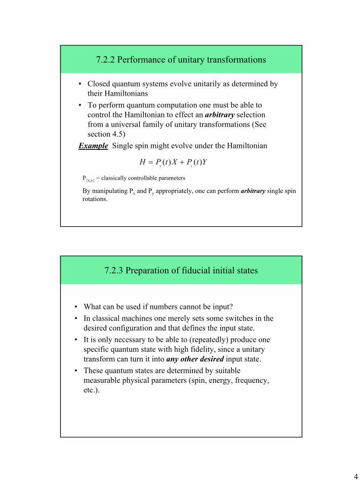
4
7.2.2 Performance of unitary transformations
• Closed quantum systems evolve unitarily as determined by their Hamiltonians
• To perform quantum computation one must be able to control the Hamiltonian to effect an arbitrary selection from a universal family of unitary transformations (See section 4.5)
Example Single spin might evolve under the Hamiltonian
YtPXtPHyx
)()( +=
Px,y = classically controllable parameters
By manipulating Px and Py appropriately, one can perform arbitrary single spin rotations.
7.2.3 Preparation of fiducial initial states
• What can be used if numbers cannot be input?• In classical machines one merely sets some switches in the
desired configuration and that defines the input state.• It is only necessary to be able to (repeatedly) produce one
specific quantum state with high fidelity, since a unitary transform can turn it into any other desired input state.
• These quantum states are determined by suitable measurable physical parameters (spin, energy, frequency, etc.).
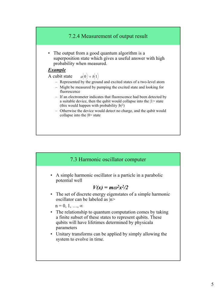
5
7.2.4 Measurement of output result
• The output from a good quantum algorithm is a superposition state which gives a useful answer with high probability when measured.
ExampleA cubit state
– Represented by the ground and excited states of a two-level atom– Might be measured by pumping the excited state and looking for
fluorescence– If an electrometer indicates that fluorescence had been detected by
a suitable device, then the qubit would collapse into the |1> state (this would happen with probability |b|2)
– Otherwise the device would detect no charge, and the qubit would collapse into the |0> state
10 ba +
7.3 Harmonic oscillator computer
• A simple harmonic oscillator is a particle in a parabolic potential well
V(x) = mω2x2/2 • The set of discrete energy eigenstates of a simple harmonic
oscillator can be labeled as |n>n = 0, 1, …, ∞
• The relationship to quantum computation comes by taking a finite subset of these states to represent qubits. These qubits will have lifetimes determined by physicala parameters
• Unitary transforms can be applied by simply allowing the system to evolve in time.
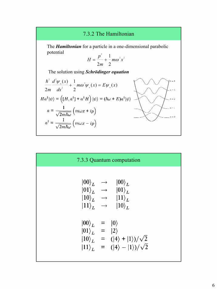
6
7.3.2 The Hamiltonian
The Hamiltonian for a particle in a one-dimensional parabolic potential
The solution using Schrödinger equation
22
2
2
1
2xm
m
pH ω+=
)()(2
1)(
22
2
22
xExmdx
xd
m nn
n ψψωψ
=+h
7.3.3 Quantum computation
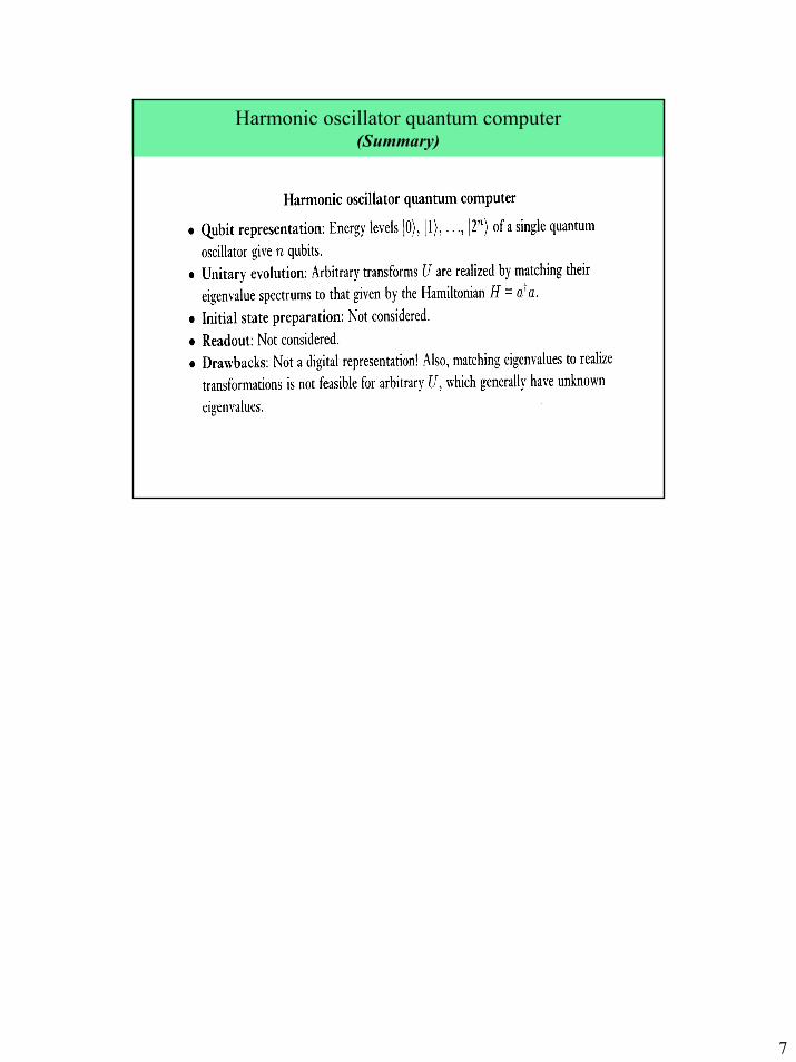
7
Harmonic oscillator quantum computer(Summary)
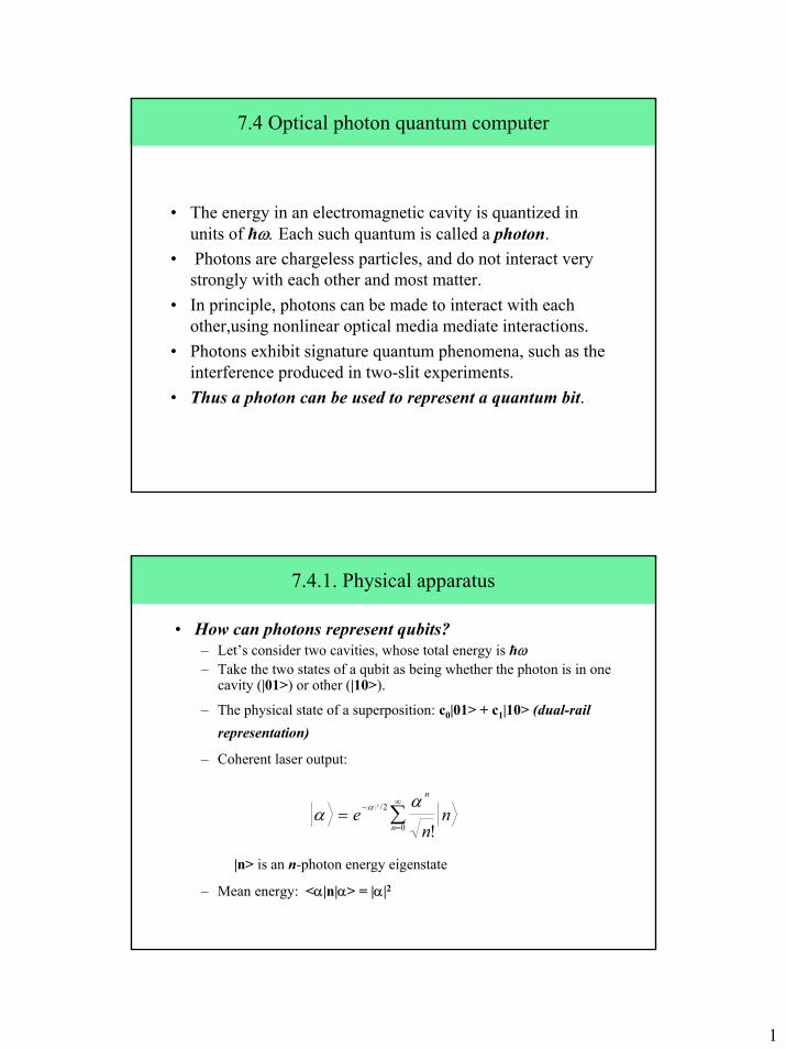
1
7.4 Optical photon quantum computer
• The energy in an electromagnetic cavity is quantized in units of ħω. Each such quantum is called a photon.
• Photons are chargeless particles, and do not interact very strongly with each other and most matter.
• In principle, photons can be made to interact with each other,using nonlinear optical media mediate interactions.
• Photons exhibit signature quantum phenomena, such as the interference produced in two-slit experiments.
• Thus a photon can be used to represent a quantum bit.
7.4.1. Physical apparatus
• How can photons represent qubits?– Let’s consider two cavities, whose total energy is ħω– Take the two states of a qubit as being whether the photon is in one
cavity (|01>) or other (|10>).
– The physical state of a superposition: c0|01> + c1|10> (dual-rail representation)
– Coherent laser output:
|n> is an n-photon energy eigenstate
– Mean energy: <α|n|α> = |α|2
∑∞
=
−=0
2/
!
2
n
n
nn
eα
α α
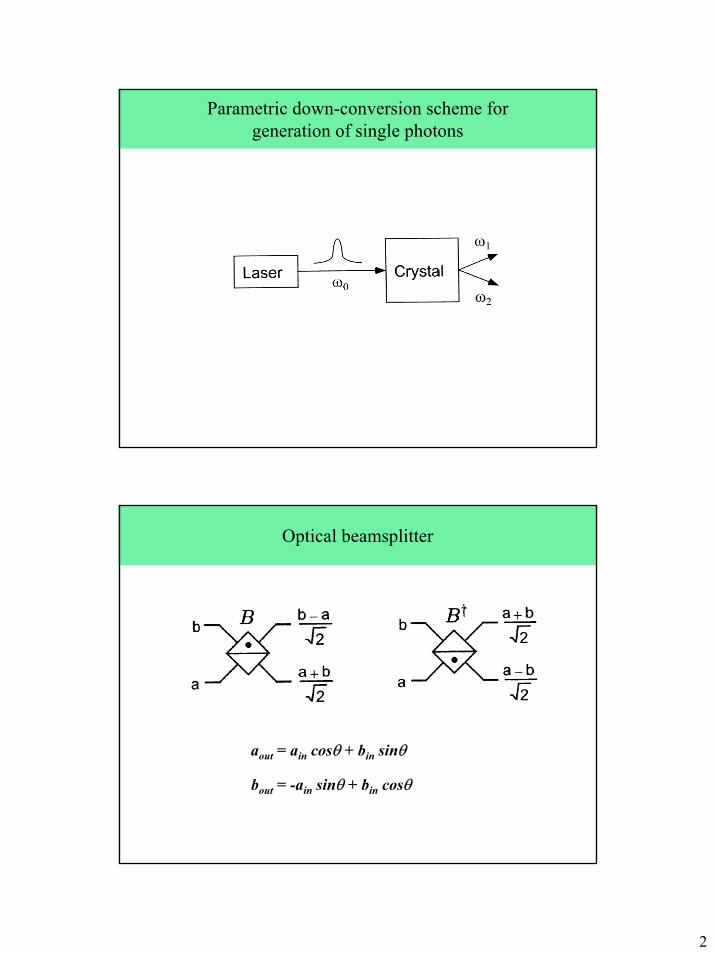
2
Parametric down-conversion scheme for generation of single photons
Optical beamsplitter
aout = ain cosθ + bin sinθ
bout = -ain sinθ + bin cosθ
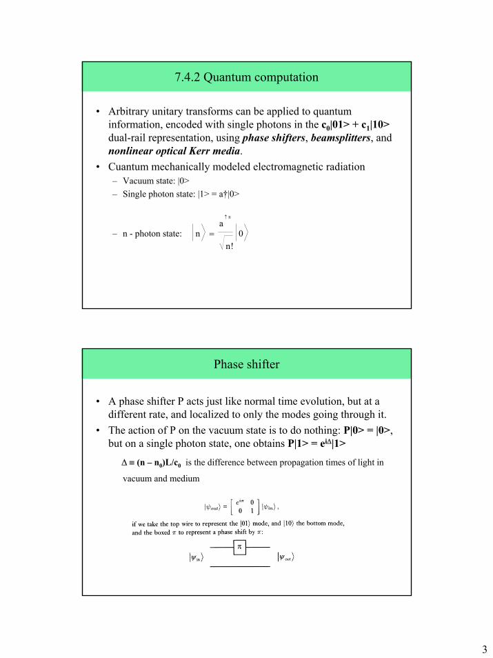
3
7.4.2 Quantum computation
• Arbitrary unitary transforms can be applied to quantum information, encoded with single photons in the c0|01> + c1|10>dual-rail representation, using phase shifters, beamsplitters, and nonlinear optical Kerr media.
• Cuantum mechanically modeled electromagnetic radiation– Vacuum state: |0>– Single photon state: |1> = a†|0>
– n - photon state: 0!n
an
n↑
=
Phase shifter
• A phase shifter P acts just like normal time evolution, but at adifferent rate, and localized to only the modes going through it.
• The action of P on the vacuum state is to do nothing: P|0> = |0>, but on a single photon state, one obtains P|1> = ei∆|1>
∆ ≡ (n – n0)L/c0 is the difference between propagation times of light in
vacuum and medium
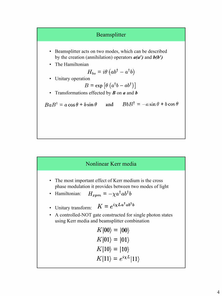
4
Beamsplitter
• Beamsplitter acts on two modes, which can be described by the creation (annihilation) operators a(a†) and b(b†)
• The Hamiltonian
• Unitary operation
• Transformations effected by B on a and b
Nonlinear Kerr media
• The most important effect of Kerr medium is the cross phase modulation it provides between two modes of light
• Hamiltonian:
• Unitary transform:• A controlled-NOT gate constructed for single photon states
using Kerr media and beamsplitter combination
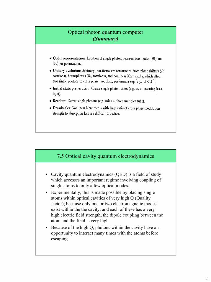
5
Optical photon quantum computer(Summary)
7.5 Optical cavity quantum electrodynamics
• Cavity quantum electrodynamics (QED) is a field of study which accesses an important regime involving coupling of single atoms to only a few optical modes.
• Experimentally, this is made possible by placing single atoms within optical cavities of very high Q (Quality factor); because only one or two electromagnetic modes exist within the the cavity, and each of these has a very high electric field strength, the dipole coupling between the atom and the field is very high
• Because of the high Q, photons within the cavity have an opportunity to interact many times with the atoms before escaping.
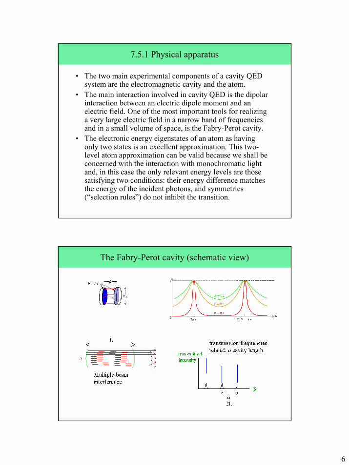
6
7.5.1 Physical apparatus
• The two main experimental components of a cavity QED system are the electromagnetic cavity and the atom.
• The main interaction involved in cavity QED is the dipolar interaction between an electric dipole moment and an electric field. One of the most important tools for realizing a very large electric field in a narrow band of frequencies and in a small volume of space, is the Fabry-Perot cavity.
• The electronic energy eigenstates of an atom as having only two states is an excellent approximation. This two-level atom approximation can be valid because we shall be concerned with the interaction with monochromatic light and, in this case the only relevant energy levels are those satisfying two conditions: their energy difference matches the energy of the incident photons, and symmetries (“selection rules”) do not inhibit the transition.
The Fabry-Perot cavity (schematic view)
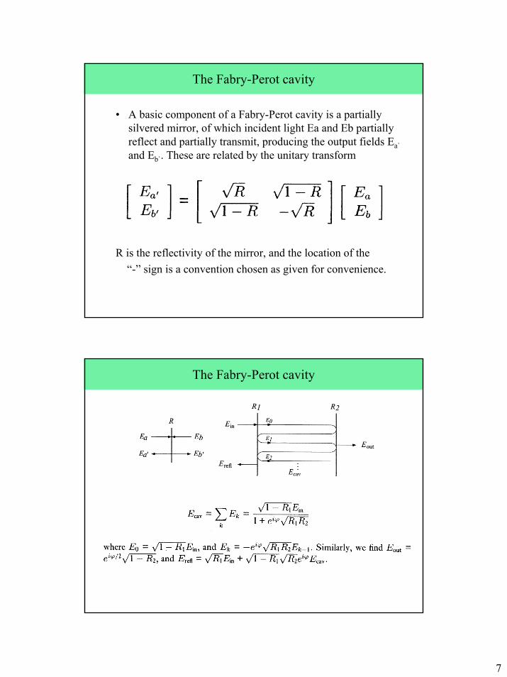
7
The Fabry-Perot cavity
• A basic component of a Fabry-Perot cavity is a partially silvered mirror, of which incident light Ea and Eb partially reflect and partially transmit, producing the output fields Ea`and Eb`. These are related by the unitary transform
R is the reflectivity of the mirror, and the location of the “-” sign is a convention chosen as given for convenience.
The Fabry-Perot cavity
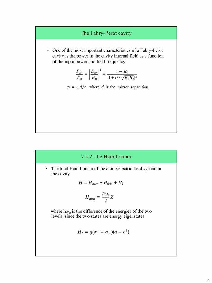
8
The Fabry-Perot cavity
• One of the most important characteristics of a Fabry-Perot cavity is the power in the cavity internal field as a function of the input power and field frequency
7.5.2 The Hamiltonian
• The total Hamiltonian of the atom×electric field system in the cavity
where ħω0 is the difference of the energies of the two levels, since the two states are energy eigenstates
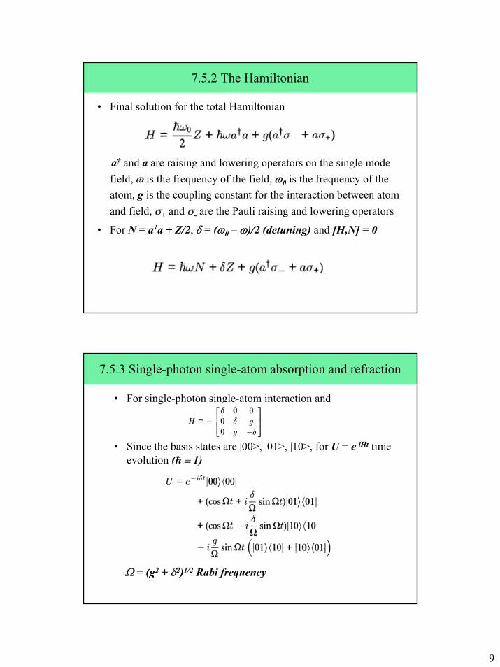
9
7.5.2 The Hamiltonian
• Final solution for the total Hamiltonian
a† and a are raising and lowering operators on the single mode field, ω is the frequency of the field, ω0 is the frequency of the atom, g is the coupling constant for the interaction between atom and field, σ+ and σ- are the Pauli raising and lowering operators
• For N = a†a + Z/2, δ = (ω0 – ω)/2 (detuning) and [H,N] = 0
7.5.3 Single-photon single-atom absorption and refraction
• For single-photon single-atom interaction and
• Since the basis states are |00>, |01>, |10>, for U = e-iHt time evolution (ħ ≡ 1)
Ω = (g2 + δ2)1/2 Rabi frequency
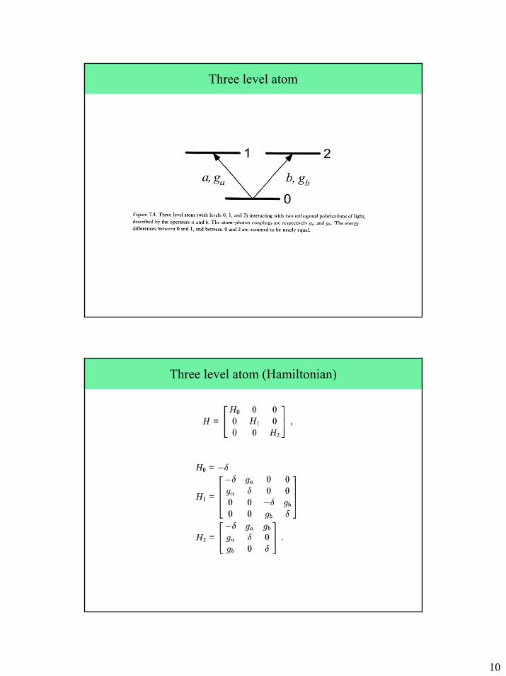
10
Three level atom
Three level atom (Hamiltonian)
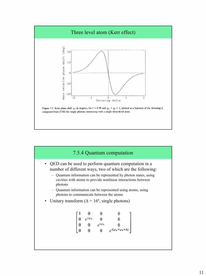
11
Three level atom (Kerr effect)
7.5.4 Quantum computation
• QED can be used to perform quantum computation in a number of different ways, two of which are the following:– Quantum information can be represented by photon states, using
cavities with atoms to provide nonlinear interactions between photons
– Quantum information can be represented using atoms, using photons to communicate between the atoms
• Unitary transform (∆ = 16º, single photons)
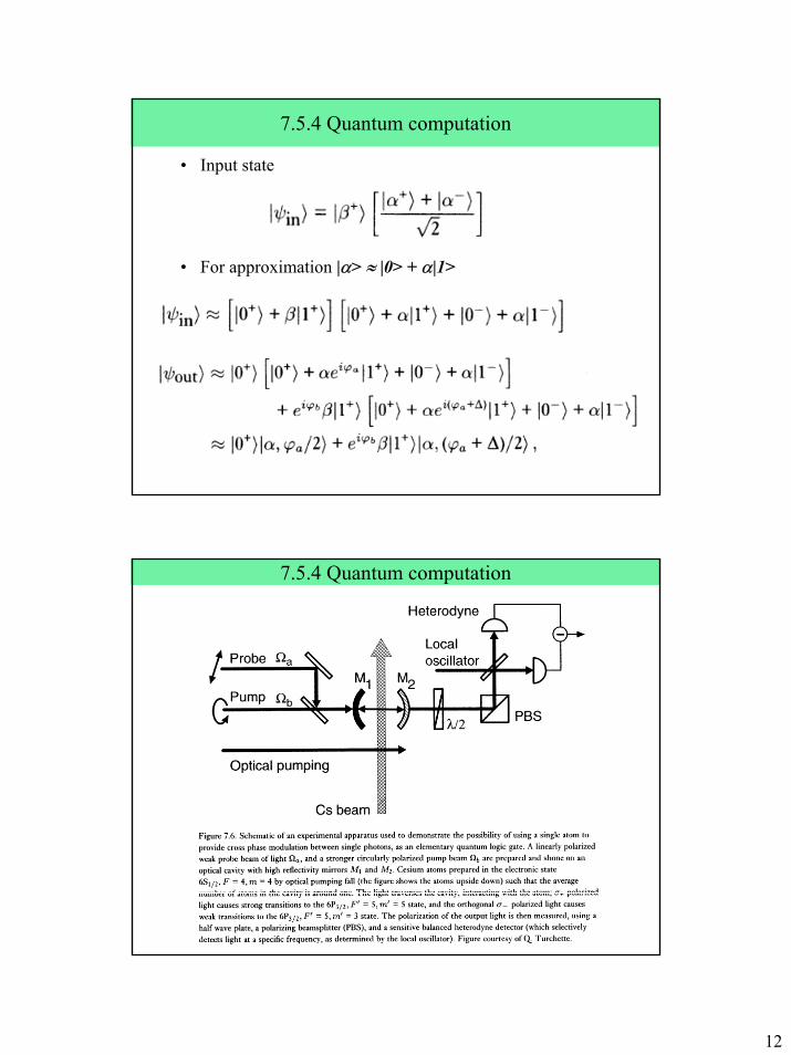
12
7.5.4 Quantum computation
• Input state
• For approximation |α> ≈ |0> + α|1>
7.5.4 Quantum computation
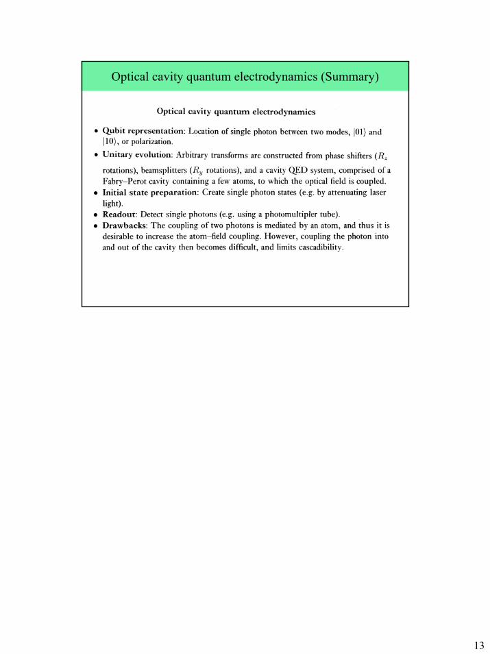
13
Optical cavity quantum electrodynamics (Summary)
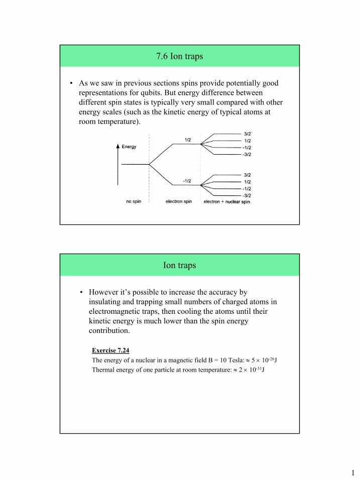
1
7.6 Ion traps
• As we saw in previous sections spins provide potentially good representations for qubits. But energy difference between different spin states is typically very small compared with other energy scales (such as the kinetic energy of typical atoms at room temperature).
Ion traps
• However it’s possible to increase the accuracy by insulating and trapping small numbers of charged atoms in electromagnetic traps, then cooling the atoms until their kinetic energy is much lower than the spin energy contribution.
Exercise 7.24The energy of a nuclear in a magnetic field B = 10 Tesla: ≈ 5 × 10-26JThermal energy of one particle at room temperature: ≈ 2 × 10-31J
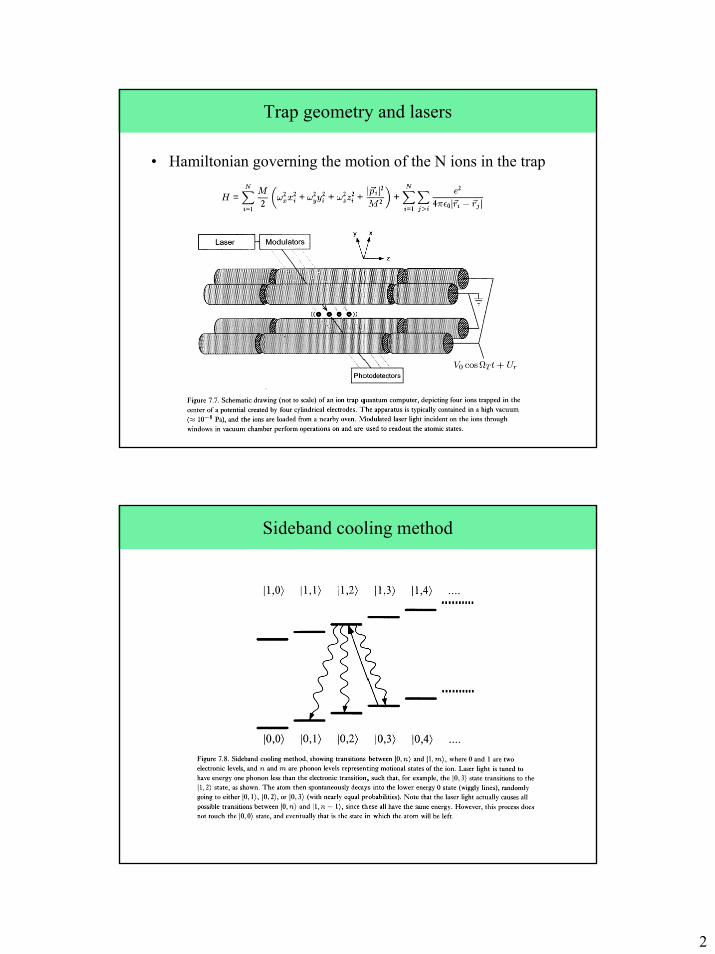
2
Trap geometry and lasers
• Hamiltonian governing the motion of the N ions in the trap
Sideband cooling method
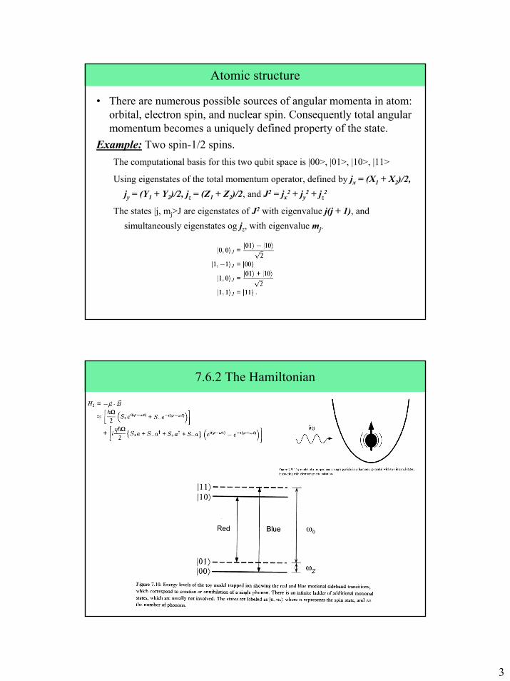
3
Atomic structure
• There are numerous possible sources of angular momenta in atom: orbital, electron spin, and nuclear spin. Consequently total angular momentum becomes a uniquely defined property of the state.
Example: Two spin-1/2 spins.The computational basis for this two qubit space is |00>, |01>, |10>, |11>
Using eigenstates of the total momentum operator, defined by jx = (X1 + X2)/2, jy = (Y1 + Y2)/2, jz = (Z1 + Z2)/2, and J2 = jx
2 + jy2 + jz
2
The states |j, mj>J are eigenstates of J2 with eigenvalue j(j + 1), and simultaneously eigenstates og jz, with eigenvalue mj.
7.6.2 The Hamiltonian
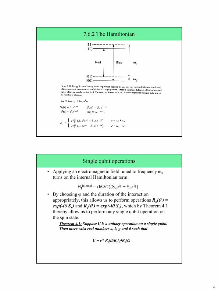
4
7.6.2 The Hamiltonian
Single qubit operations
• Applying an electromagnetic field tuned to frequency ω0turns on the internal Hamiltonian term
HIinternal = (ħΩ/2)(S+eiϕ + S-e-iϕ)
• By choosing ϕ and the duration of the interaction appropriately, this allows us to perform operations Rx(θ ) = exp(-iθ Sx) and Ry(θ ) = exp(-iθ Sy), which by Theorem 4.1 thereby allow us to perform any single qubit operation on the spin state. – Theorem 4.1: Suppose U is a unitary operation on a single qubit.
Then there exist real numbers a, b, g and d such that
U = eiα Rz(β)Ry(γ)Rz(δ)
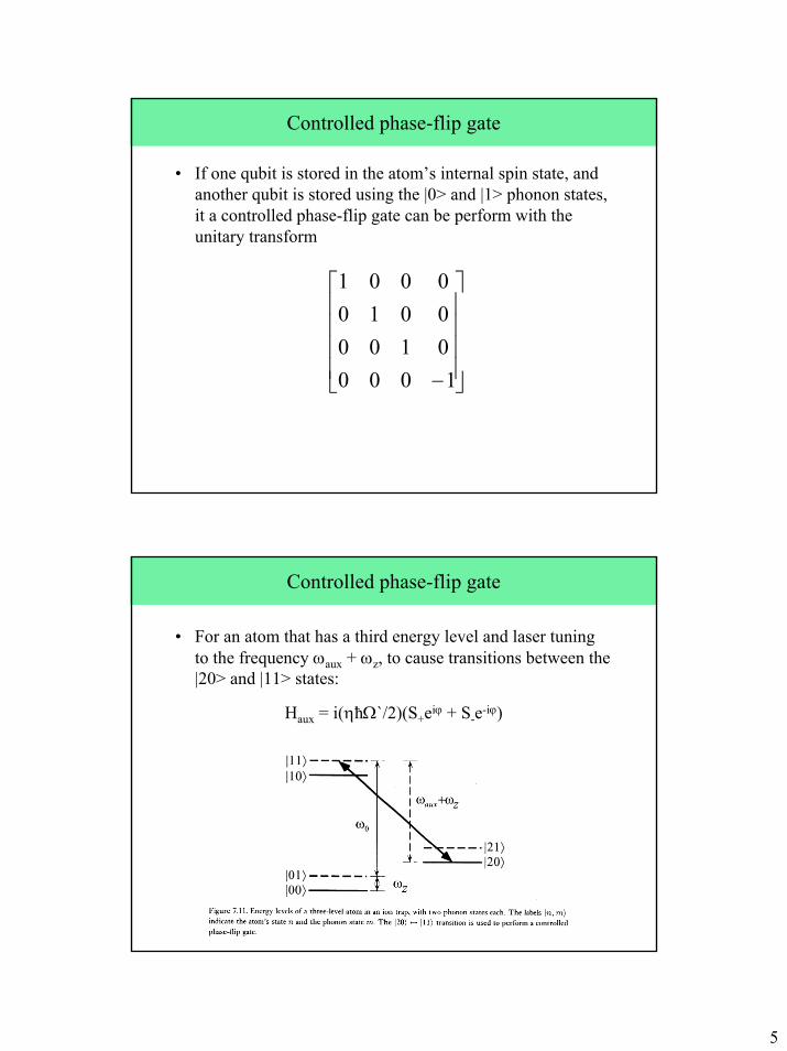
5
Controlled phase-flip gate
• If one qubit is stored in the atom’s internal spin state, and another qubit is stored using the |0> and |1> phonon states, it a controlled phase-flip gate can be perform with the unitary transform
−1000010000100001
Controlled phase-flip gate
• For an atom that has a third energy level and laser tuning to the frequency ωaux + ωz, to cause transitions between the |20> and |11> states:
Haux = i(ηħΩ`/2)(S+eiϕ + S-e-iϕ)
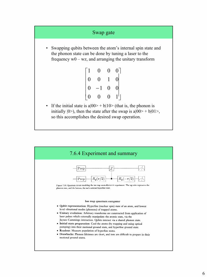
6
Swap gate
• Swapping qubits between the atom’s internal spin state and the phonon state can be done by tuning a laser to the frequency w0 – wz, and arranging the unitary transform
• If the initial state is a|00> + b|10> (that is, the phonon is initially |0>), then the state after the swap is a|00> + b|01>, so this accomplishes the desired swap operation.
−1000001001000001
7.6.4 Experiment and summary
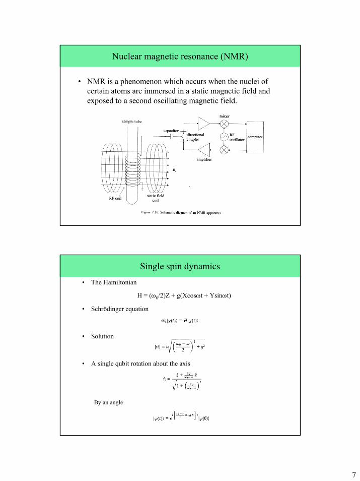
7
Nuclear magnetic resonance (NMR)
• NMR is a phenomenon which occurs when the nuclei of certain atoms are immersed in a static magnetic field and exposed to a second oscillating magnetic field.
Single spin dynamics• The Hamiltonian
H = (ω0/2)Z + g(Xcosωt + Ysinωt)
• Schrödinger equation
• Solution
• A single qubit rotation about the axis
By an angle
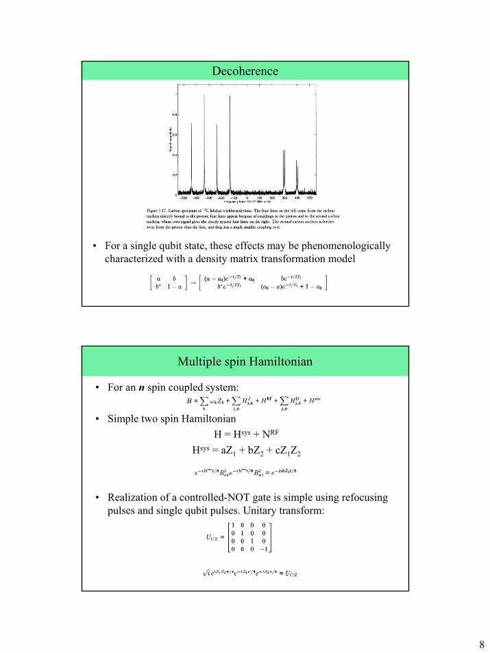
8
Decoherence
• For a single qubit state, these effects may be phenomenologically characterized with a density matrix transformation model
Multiple spin Hamiltonian
• For an n spin coupled system:
• Simple two spin HamiltonianH = Hsys + NRF
Hsys = aZ1 + bZ2 + cZ1Z2
• Realization of a controlled-NOT gate is simple using refocusing pulses and single qubit pulses. Unitary transform:
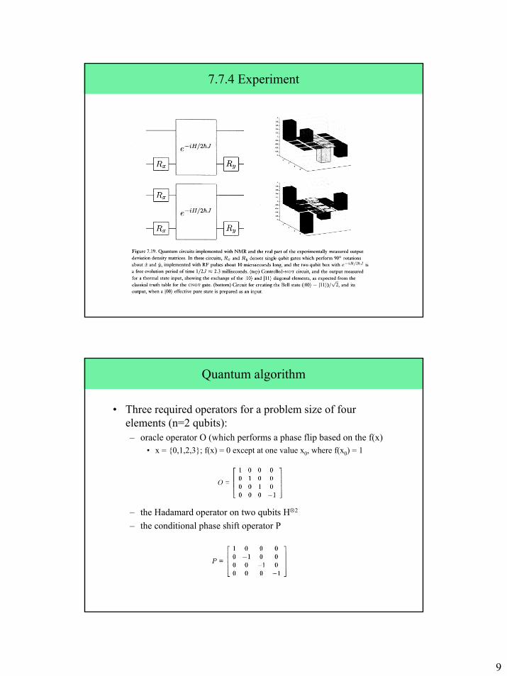
9
7.7.4 Experiment
Quantum algorithm
• Three required operators for a problem size of four elements (n=2 qubits): – oracle operator O (which performs a phase flip based on the f(x)
• x = 0,1,2,3; f(x) = 0 except at one value x0, where f(x0) = 1
– the Hadamard operator on two qubits H⊗2
– the conditional phase shift operator P
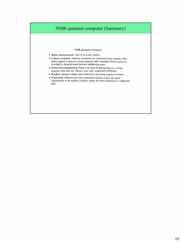
10
NMR quantum computer (Summary)
Quantum Computational Quantum Computational IntelligenceIntelligence
OutlineOverviewQuantum search (revisited)
Extensions:Search over arbitrary initial amplitude distributionsQuantum Associative Memory (QuAM)
Beyond Phase AmplificationQuAM - UpgradedCompetitive Learning
Conclusions
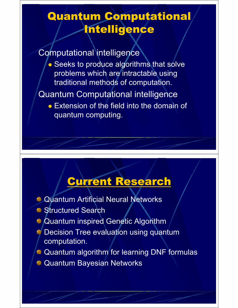
Quantum Computational Intelligence
Computational intelligenceSeeks to produce algorithms that solve problems which are intractable using traditional methods of computation.
Quantum Computational intelligenceExtension of the field into the domain of quantum computing.
CurrentCurrent ResearchResearchQuantum Artificial Neural NetworksStructured SearchQuantum inspired Genetic Algorithm Decision Tree evaluation using quantum computation.Quantum algorithm for learning DNF formulasQuantum Bayesian Networks
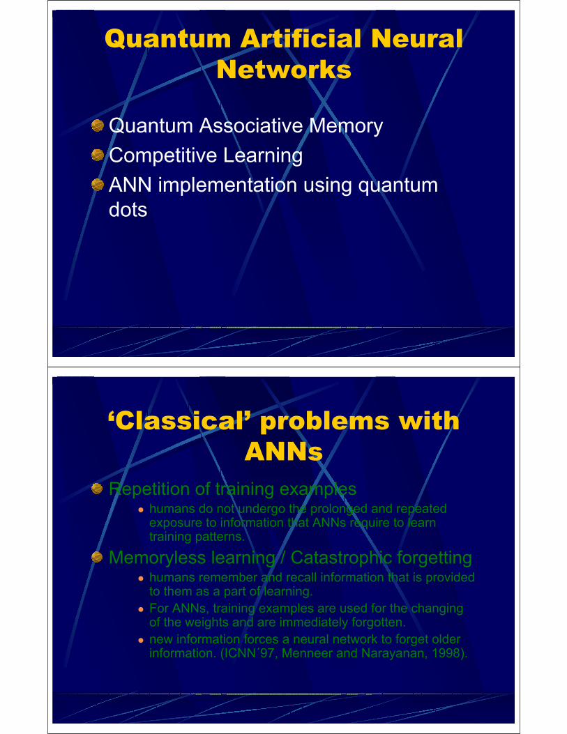
Quantum Artificial Neural Networks
Quantum Associative MemoryCompetitive LearningANN implementation using quantum dots
‘Classical’ problems with ANNs
Repetition of training examples humans do not undergo the prolonged and repeated exposure to information that ANNs require to learn training patterns.
Memoryless learning / Catastrophic forgettinghumans remember and recall information that is provided to them as a part of learning. For ANNs, training examples are used for the changing of the weights and are immediately forgotten. new information forces a neural network to forget older information. (ICNN´97, Menneer and Narayanan, 1998).
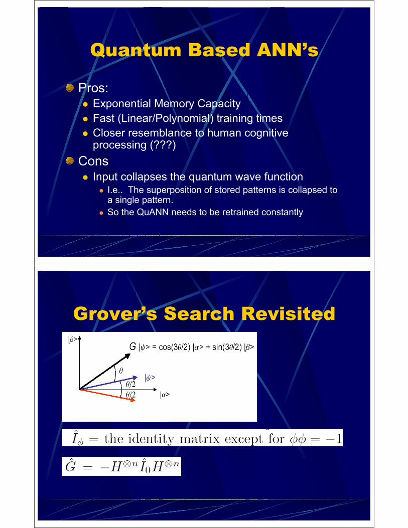
Quantum Based ANN’s
Pros:Exponential Memory CapacityFast (Linear/Polynomial) training timesCloser resemblance to human cognitive processing (???)
ConsInput collapses the quantum wave function
I.e.. The superposition of stored patterns is collapsed to a single pattern.So the QuANN needs to be retrained constantly
Grover’s Search Revisited
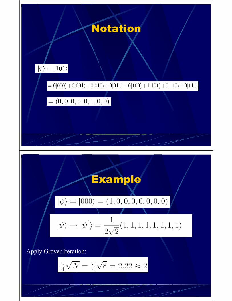
Notation
Example
Apply Grover Iteration:
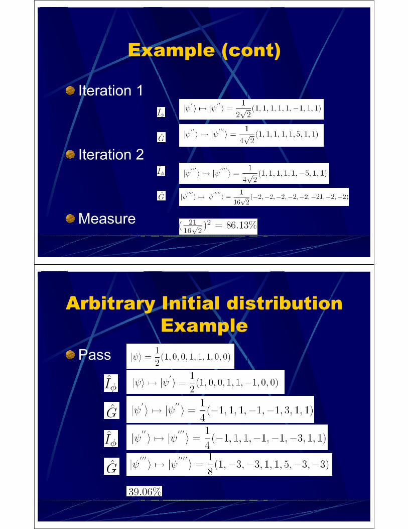
Example (cont)
Iteration 1
Iteration 2
Measure
Arbitrary Initial distribution Example
Pass
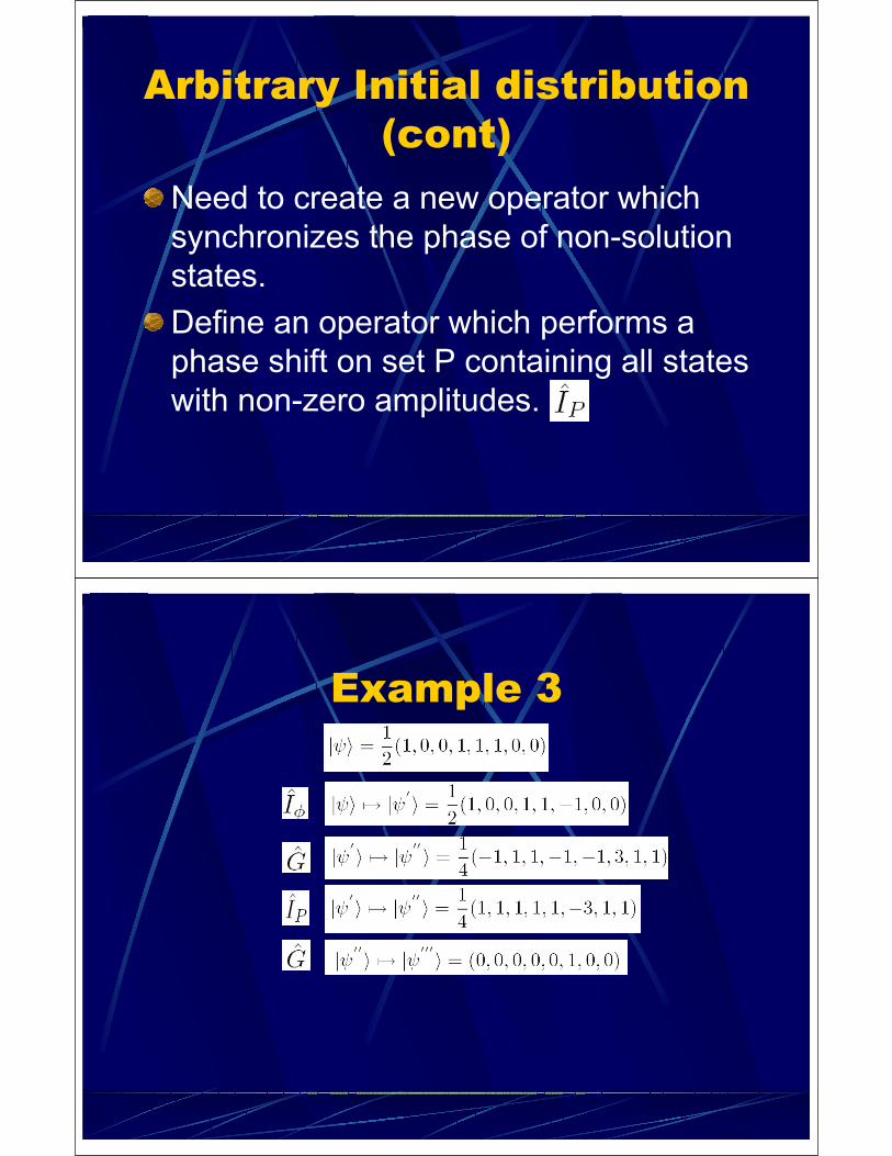
Arbitrary Initial distribution (cont)
Need to create a new operator which synchronizes the phase of non-solution states.Define an operator which performs a phase shift on set P containing all states with non-zero amplitudes.
Example 3
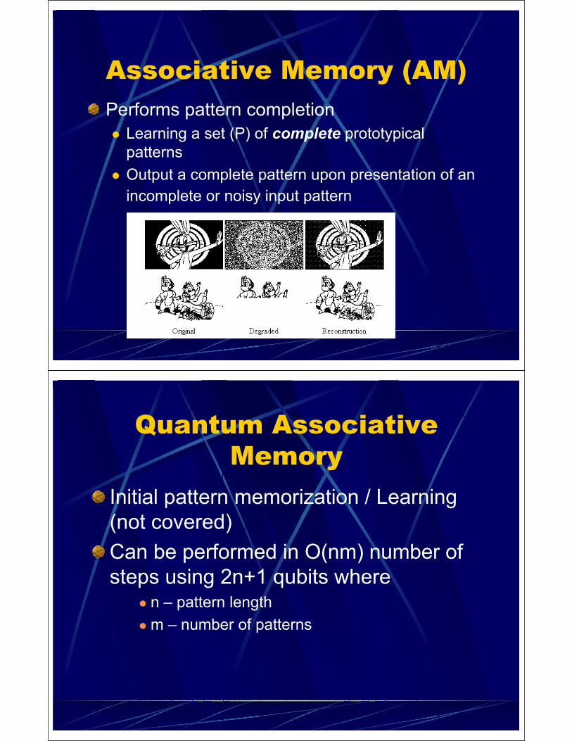
Associative Memory (AM)Performs pattern completion
Learning a set (P) of complete prototypicalpatternsOutput a complete pattern upon presentation of an incomplete or noisy input pattern
Quantum Associative Memory
Initial pattern memorization / Learning (not covered)Can be performed in O(nm) number of steps using 2n+1 qubits where
n – pattern lengthm – number of patterns
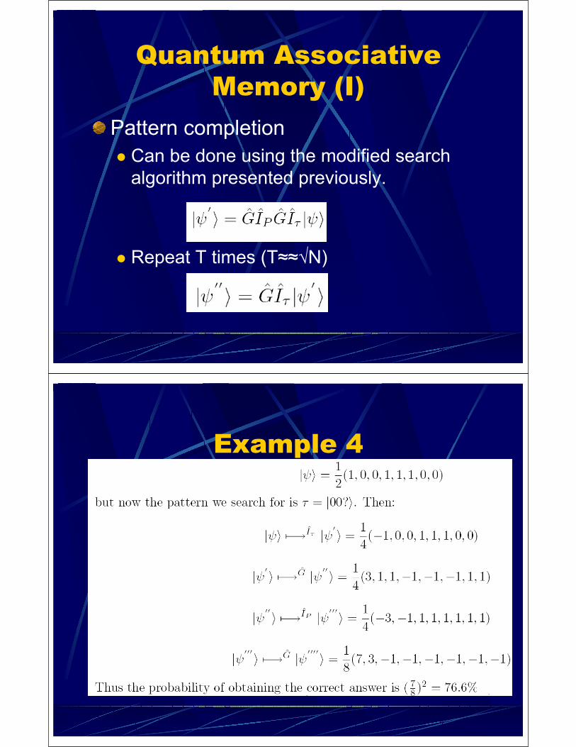
Quantum Associative Memory (I)
Pattern completionCan be done using the modified search algorithm presented previously.
Repeat T times (T N)
Example 4
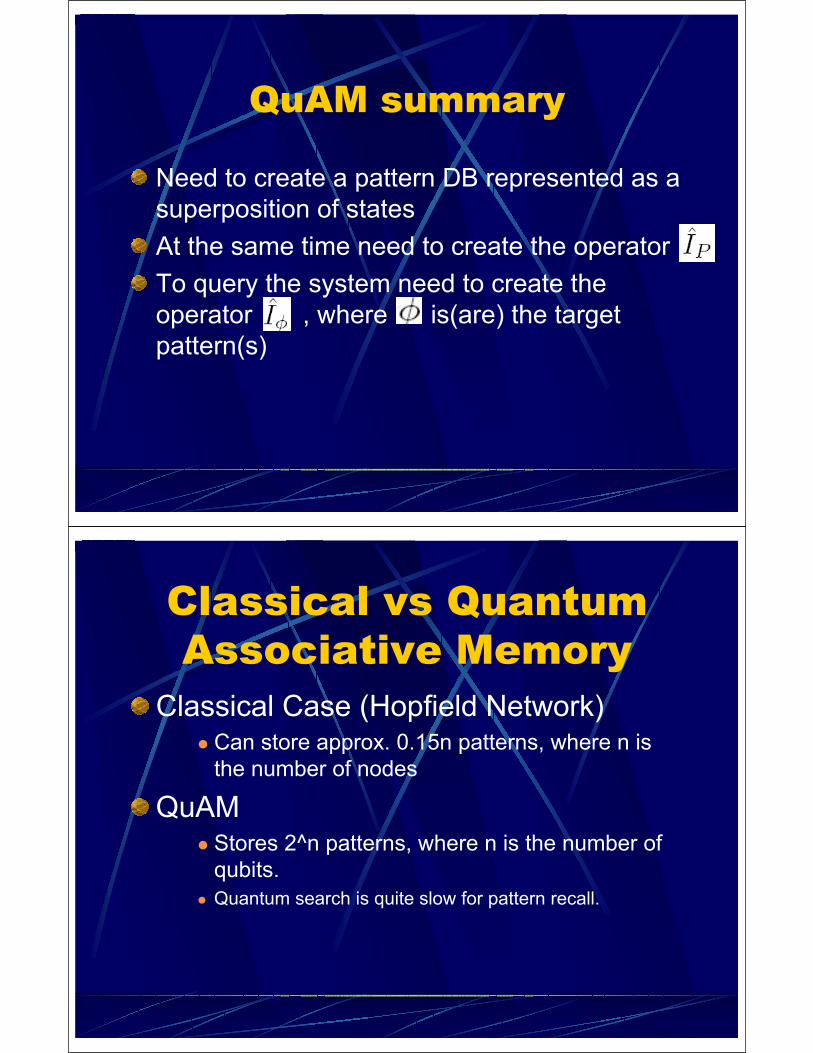
QuAM summary
Need to create a pattern DB represented as a superposition of statesAt the same time need to create the operator To query the system need to create the operator , where is(are) the target pattern(s)
Classical vs Quantum Associative Memory
Classical Case (Hopfield Network)Can store approx. 0.15n patterns, where n is the number of nodes
QuAMStores 2^n patterns, where n is the number of qubits.Quantum search is quite slow for pattern recall.
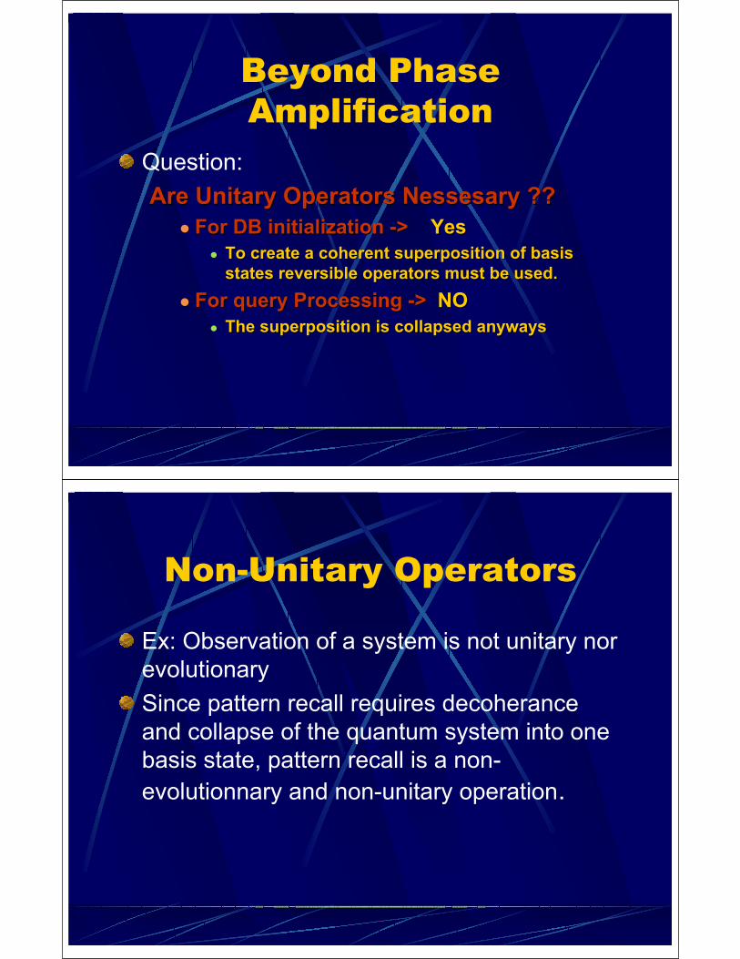
Beyond Phase Amplification
Question:Are Unitary Operators Nessesary ??Are Unitary Operators Nessesary ??
For DB initialization For DB initialization -->> YesYesTo create a coherent superposition of basis To create a coherent superposition of basis states reversible operators must be used.states reversible operators must be used.
For query Processing For query Processing -->> NONOThe superposition is collapsed anywaysThe superposition is collapsed anyways
Non-Unitary Operators
Ex: Observation of a system is not unitary nor evolutionarySince pattern recall requires decoherance and collapse of the quantum system into one basis state, pattern recall is a non-evolutionnary and non-unitary operation.
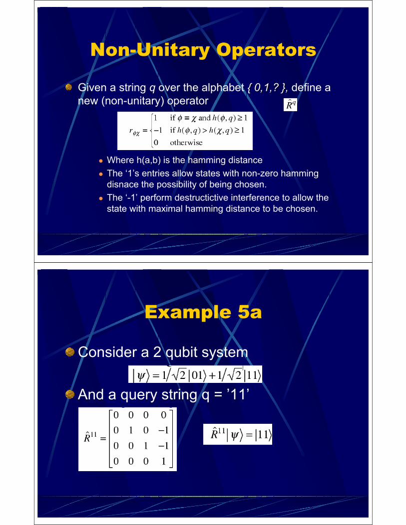
Non-Unitary Operators
Given a string q over the alphabet 0,1,? , 0,1,? , define a new (non-unitary) operator
Where h(a,b) is the hamming distanceThe ‘1’s entries allow states with non-zero hamming disnace the possibility of being chosen.The ‘-1’ perform destructictive interference to allow the state with maximal hamming distance to be chosen.
Example 5a
Consider a 2 qubit system
And a query string q = ’11’
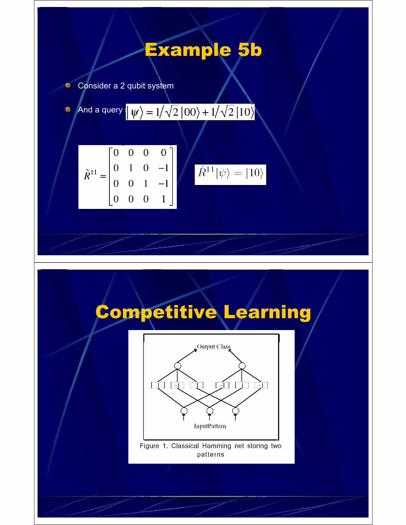
Example 5b
Consider a 2 qubit system
And a query string q = ’11’
Competitive Learning
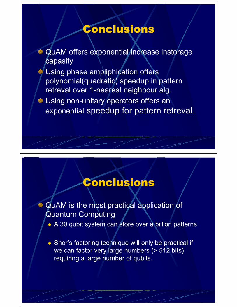
Conclusions
QuAM offers exponential increase instorage capasityUsing phase ampliphication offers polynomial(quadratic) speedup in pattern retreval over 1-nearest neighbour alg.Using non-unitary operators offers an exponential speedup for pattern retreval.
Conclusions
QuAM is the most practical application of Quantum Computing
A 30 qubit system can store over a billion patterns
Shor’s factoring technique will only be practical if we can factor very large numbers (> 512 bits) requiring a large number of qubits.
References
http://www.cic.unb.br/docentes/weigang/qc/aci.html
http://www.cs.ualberta.ca/~ilya/courses/c605-QC/Refs.pdf
Final Thoughts
Prof. Sham: Well, we factored number 15 into 3 times 5. It was a thorny problem, but, by Jove, we did it. We started building our NMRcomputer in 1997 with a 5-million-dollar grant from DARPA. So it took 5 years, a few million dollars, and much hard work to build ourroom sized computer. But just think how powerful it is! And according to theory, NMR computers have tremendous growth potential. They can have as many as 10 qubits!Reporter: Could you please tell us something about your future plans? Prof. Sham: Well. I plan to continue publishing in Nature Magazine. Another exciting development is that I plan to add one more qubit to NMR computers in the next few years. We've won another 3-million-dollar grant from DARPA to continue our work. Isn't our government just great! We can't wait to start factoring number 18.
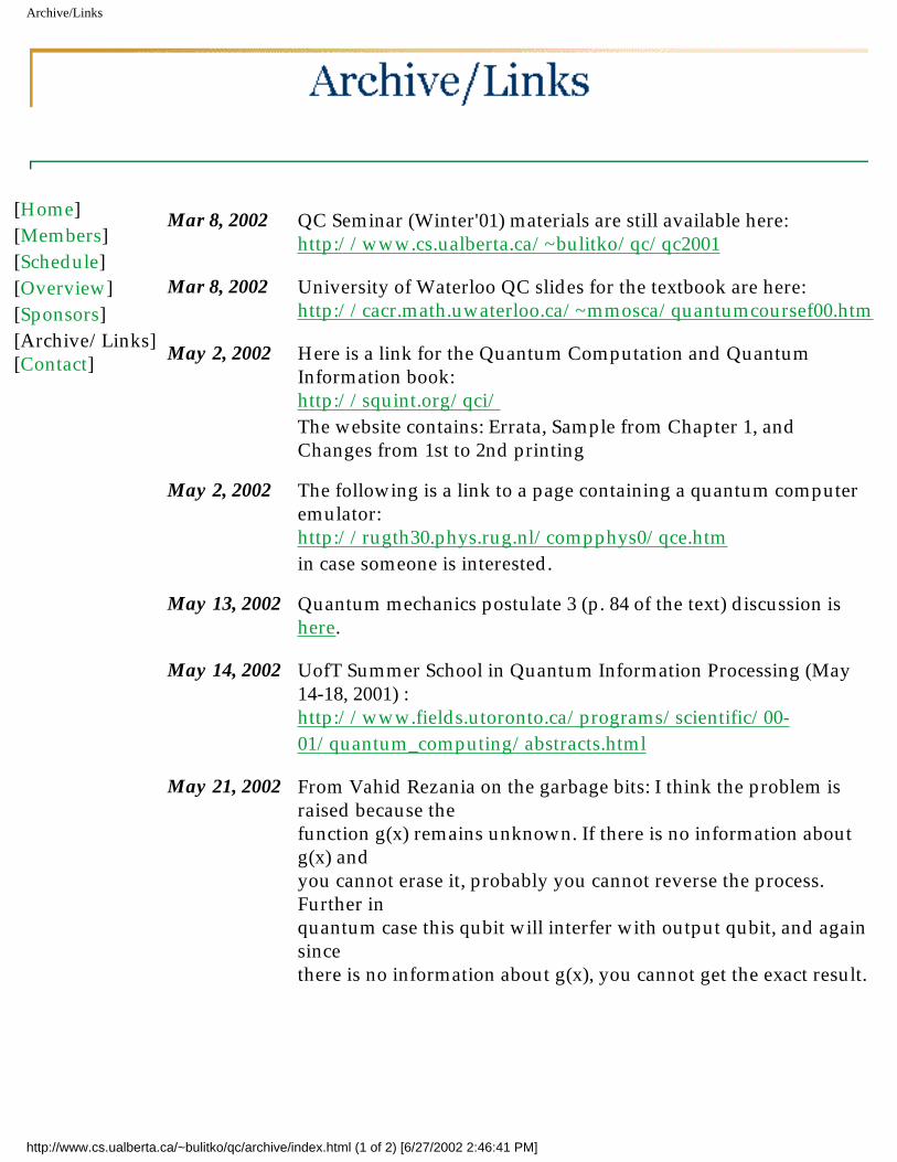
Archive/Links
[Home][Members][Schedule][Overview][Sponsors][Archive/Links][Contact]
Mar 8, 2002 QC Seminar (Winter'01) materials are still available here: http://www.cs.ualberta.ca/~bulitko/qc/qc2001
Mar 8, 2002 University of Waterloo QC slides for the textbook are here: http://cacr.math.uwaterloo.ca/~mmosca/quantumcoursef00.htm
May 2, 2002 Here is a link for the Quantum Computation and Quantum Information book:http://squint.org/qci/ The website contains: Errata, Sample from Chapter 1, and Changes from 1st to 2nd printing
May 2, 2002 The following is a link to a page containing a quantum computer emulator:http://rugth30.phys.rug.nl/compphys0/qce.htm in case someone is interested.
May 13, 2002 Quantum mechanics postulate 3 (p. 84 of the text) discussion is here.
May 14, 2002 UofT Summer School in Quantum Information Processing (May 14-18, 2001) : http://www.fields.utoronto.ca/programs/scientific/00-01/quantum_computing/abstracts.html
May 21, 2002 From Vahid Rezania on the garbage bits: I think the problem is raised because the function g(x) remains unknown. If there is no information about g(x) and you cannot erase it, probably you cannot reverse the process. Further in quantum case this qubit will interfer with output qubit, and again since there is no information about g(x), you cannot get the exact result.
http://www.cs.ualberta.ca/~bulitko/qc/archive/index.html (1 of 2) [6/27/2002 2:46:41 PM]

Archive/Links
May 22, 2002 From Dan Tzur on why garbage bits are bad : Well, I don't know yet, but I found this webpage that could lead to an answer:
http://arxiv.org/PS_cache/quant-ph/pdf/9806/9806084.pdf
and this:
http://qso.lanl.gov/~zalka/QC/QC.html
Home | Members | Schedule | Overview | Sponsors | Archive/Links | Contact
Copyright (C) by V.Bulitko, 2000-2002. All Rights Reserved.For problems or questions regarding this web contact V.Bulitko.
Last updated: 03/08/02.
http://www.cs.ualberta.ca/~bulitko/qc/archive/index.html (2 of 2) [6/27/2002 2:46:41 PM]
Contact Us
[Home][Members][Schedule][Overview][Sponsors][Archive/Links][Contact]
Name Prof. Vadim Bulitko (summer school chair)
Mailing Address
Department of Computing ScienceUniversity of AlbertaEdmonton, Alberta, T6G 2H1CANADA
Fax (780) 492-1071
WWW http://www.cs.ualberta.ca/~bulitko
E-Mail [email protected]
Home | Members | Schedule | Overview | Sponsors | Archive/Links | Contact
Copyright (C) by V.Bulitko, 2000-2002. All Rights Reserved.For problems or questions regarding this web contact V.Bulitko.
Last updated: 03/08/02.
http://www.cs.ualberta.ca/~bulitko/qc/contact/index.html [6/27/2002 2:46:52 PM]
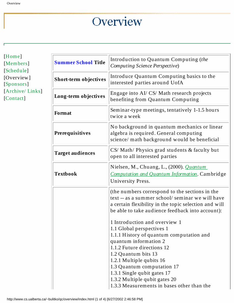
Overview
[Home][Members][Schedule][Overview][Sponsors][Archive/Links][Contact]
Summer School Title Introduction to Quantum Computing (the Computing Science Perspective)
Short-term objectives Introduce Quantum Computing basics to the interested parties around UofA
Long-term objectives Engage into AI/CS/Math research projects benefiting from Quantum Computing
Format Seminar-type meetings, tentatively 1-1.5 hours twice a week
PrerequisitivesNo background in quantum mechanics or linear algebra is required. General computing science/math background would be beneficial
Target audiences CS/Math/Physics grad students & faculty but open to all interested parties
TextbookNielsen, M., Chuang, L., (2000). Quantum Computation and Quantum Information. Cambridge University Press.
(the numbers correspond to the sections in the text -- as a summer school/seminar we will have a certain flexibility in the topic selection and will be able to take audience feedback into account):
1 Introduction and overview 1 1.1 Global perspectives 1 1.1.1 History of quantum computation and quantum information 2 1.1.2 Future directions 12 1.2 Quantum bits 13 1.2.1 Multiple qubits 16 1.3 Quantum computation 17 1.3.1 Single qubit gates 17 1.3.2 Multiple qubit gates 20 1.3.3 Measurements in bases other than the
http://www.cs.ualberta.ca/~bulitko/qc/overview/index.html (1 of 4) [6/27/2002 2:46:58 PM]
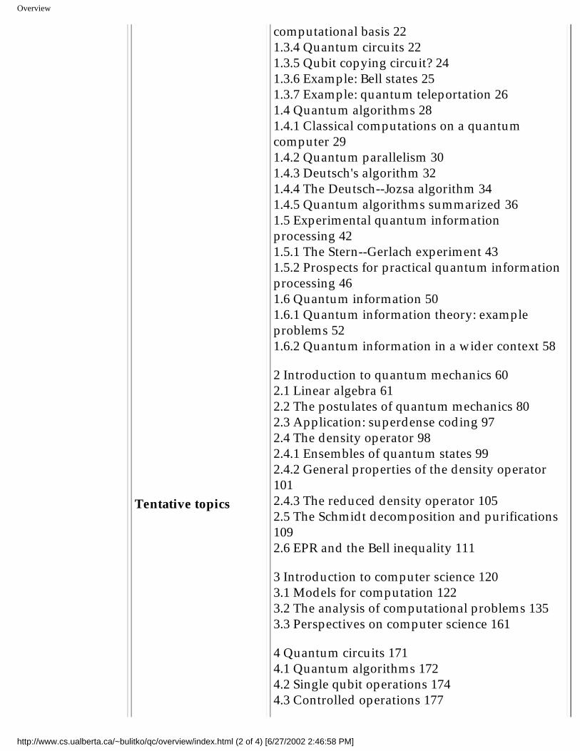
Overview
Tentative topics
computational basis 22 1.3.4 Quantum circuits 22 1.3.5 Qubit copying circuit? 24 1.3.6 Example: Bell states 25 1.3.7 Example: quantum teleportation 26 1.4 Quantum algorithms 28 1.4.1 Classical computations on a quantum computer 29 1.4.2 Quantum parallelism 30 1.4.3 Deutsch's algorithm 32 1.4.4 The Deutsch--Jozsa algorithm 34 1.4.5 Quantum algorithms summarized 36 1.5 Experimental quantum information processing 42 1.5.1 The Stern--Gerlach experiment 43 1.5.2 Prospects for practical quantum information processing 46 1.6 Quantum information 50 1.6.1 Quantum information theory: example problems 52 1.6.2 Quantum information in a wider context 58
2 Introduction to quantum mechanics 60 2.1 Linear algebra 61 2.2 The postulates of quantum mechanics 80 2.3 Application: superdense coding 97 2.4 The density operator 98 2.4.1 Ensembles of quantum states 99 2.4.2 General properties of the density operator 101 2.4.3 The reduced density operator 105 2.5 The Schmidt decomposition and purifications 109 2.6 EPR and the Bell inequality 111
3 Introduction to computer science 120 3.1 Models for computation 122 3.2 The analysis of computational problems 135 3.3 Perspectives on computer science 161
4 Quantum circuits 171 4.1 Quantum algorithms 172 4.2 Single qubit operations 174 4.3 Controlled operations 177
http://www.cs.ualberta.ca/~bulitko/qc/overview/index.html (2 of 4) [6/27/2002 2:46:58 PM]
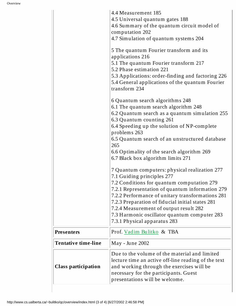
Overview
4.4 Measurement 185 4.5 Universal quantum gates 188 4.6 Summary of the quantum circuit model of computation 202 4.7 Simulation of quantum systems 204
5 The quantum Fourier transform and its applications 216 5.1 The quantum Fourier transform 217 5.2 Phase estimation 221 5.3 Applications: orderfinding and factoring 226 5.4 General applications of the quantum Fourier transform 234
6 Quantum search algorithms 248 6.1 The quantum search algorithm 248 6.2 Quantum search as a quantum simulation 255 6.3 Quantum counting 261 6.4 Speeding up the solution of NPcomplete problems 263 6.5 Quantum search of an unstructured database 265 6.6 Optimality of the search algorithm 269 6.7 Black box algorithm limits 271
7 Quantum computers: physical realization 277 7.1 Guiding principles 277 7.2 Conditions for quantum computation 279 7.2.1 Representation of quantum information 279 7.2.2 Performance of unitary transformations 281 7.2.3 Preparation of fiducial initial states 281 7.2.4 Measurement of output result 282 7.3 Harmonic oscillator quantum computer 283 7.3.1 Physical apparatus 283
Presenters Prof. Vadim Bulitko & TBA
Tentative time-line May - June 2002
Class participation
Due to the volume of the material and limited lecture time an active off-line reading of the text and working through the exercises will be necessary for the participants. Guest presentations will be welcome.
http://www.cs.ualberta.ca/~bulitko/qc/overview/index.html (3 of 4) [6/27/2002 2:46:58 PM]

Overview
Registration
No official UofA registration is required. Simply e-mail to the school chair if you are [seriously] interested in attending and/or presenting/teaching.
Home | Members | Schedule | Overview | Sponsors | Archive/Links | Contact
Copyright (C) by V.Bulitko, 2000-2002. All Rights Reserved.For problems or questions regarding this web contact V.Bulitko.
Last updated: 03/08/02.
http://www.cs.ualberta.ca/~bulitko/qc/overview/index.html (4 of 4) [6/27/2002 2:46:58 PM]